The Dogleg and Steihaug Methods

Lecture 7, Continuous Optimisation

Oxford University Computing Laboratory, HT 2005

Dr Raphael Hauser (hauser@comlab.ox.ac.uk)

Variants of Trust-Region Methods:

0. Different choices of trust region Rk, for example using balls

defined by the norms ‖ · ‖1 or ‖ · ‖∞. Not further pursued.

I. Choosing the model function mk. We chose

mk(x) = f(xk) + ∇f(xk)T(x − xk) +

1

2(x − xk)

TBk(x − xk).

Leaves choice in determining Bk. Further discussed below.

II. Approximate calculation of

yk+1 ≈ arg miny∈Rk

mk(y). (1)

Further discussed below.

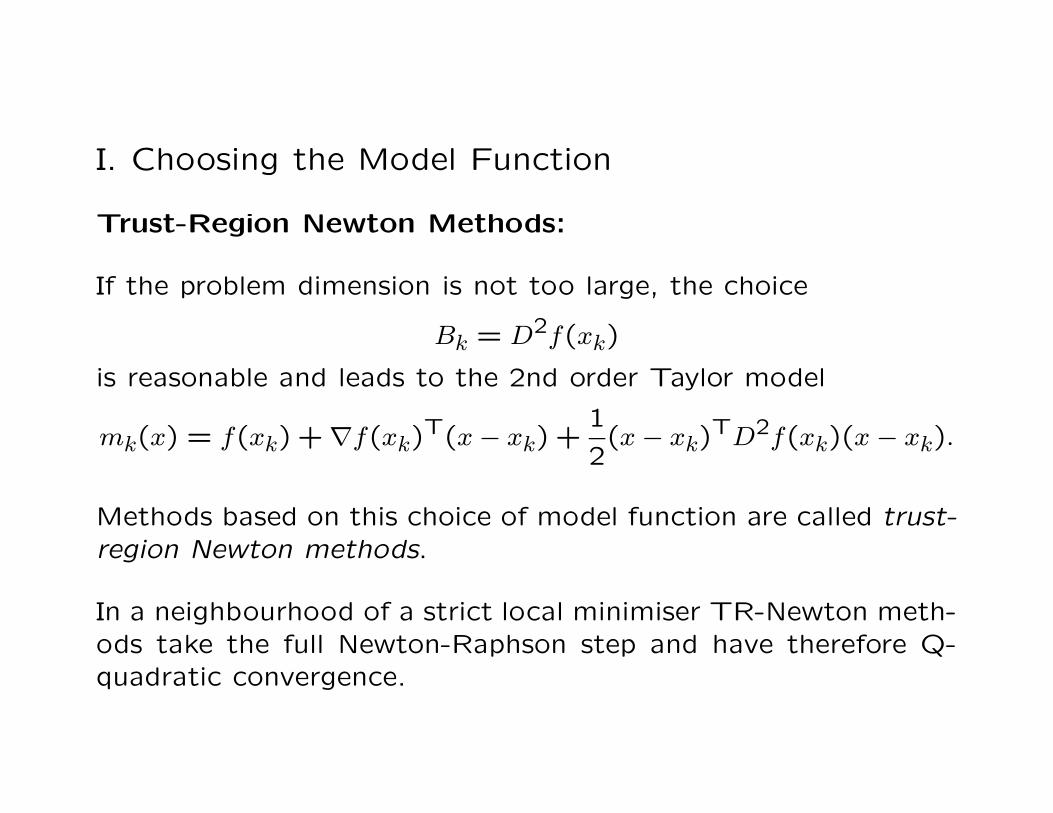
I. Choosing the Model Function

Trust-Region Newton Methods:

If the problem dimension is not too large, the choice

Bk = D2f(xk)

is reasonable and leads to the 2nd order Taylor model

mk(x) = f(xk) + ∇f(xk)T(x − xk) +

1

2(x − xk)

TD2f(xk)(x − xk).

Methods based on this choice of model function are called trust-

region Newton methods.

In a neighbourhood of a strict local minimiser TR-Newton meth-

ods take the full Newton-Raphson step and have therefore Q-

quadratic convergence.

Trust-region Newton methods are not simply the Newton-Raphson

method with an additional step-size restriction!

• TR-Newton is a descent method, whereas this is not guar-

anteed for Newton-Raphson.

• In TR-Newton, usually yk+1 − xk 6∼ −(D2f(xk))−1∇f(xk), as

yk+1 is not obtained via a line search but by optimising (1).

• In TR-Newton the update yk+1 is well-defined even when

D2f(xk) is singular.

Trust-Region Quasi-Newton Methods:

When the problem dimension n is large, the natural choice for

the model function mk is to use quasi-Newton updates for the

approximate Hessians Bk.

Such methods are called trust-region quasi-Newton.

In a neighbourhood of a strict local minimiser TR-quasi-Newton

methods take the full quasi-Newton step and have therefore Q-

superlinear convergence.

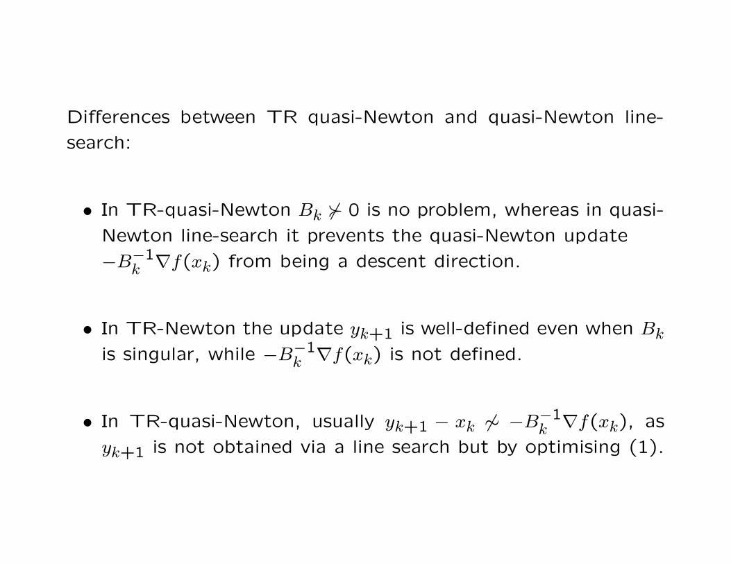
Differences between TR quasi-Newton and quasi-Newton line-

search:

• In TR-quasi-Newton Bk 6� 0 is no problem, whereas in quasi-

Newton line-search it prevents the quasi-Newton update

−B−1k ∇f(xk) from being a descent direction.

• In TR-Newton the update yk+1 is well-defined even when Bk

is singular, while −B−1k ∇f(xk) is not defined.

• In TR-quasi-Newton, usually yk+1 − xk 6∼ −B−1k ∇f(xk), as

yk+1 is not obtained via a line search but by optimising (1).

II. Solving the Trust-Region Subproblem

The Dogleg Method:

This method is very simple and cheap to compute, but it works

only when Bk � 0. Therefore, BFGS updates for Bk are a good,

but the method is not applicable for SR1 updates.

Motivation: let

x(∆) := arg min{x∈Rn:‖x−xk‖≤∆}

mk(x).

If Bk � 0 then ∆ 7→ x(∆) describes a curvilinear path from

x(0) = xk to the exact minimiser of the unconstrained problem

minx∈Rn mk(x), that is, to the quasi-Newton point

yqnk = xk − B−1

k ∇f(xk).

Idea:

• Replace the curvilinear path ∆ 7→ x(∆) by a polygonal path

τ 7→ y(τ).

• Determine yk+1 as the minimiser of mk(y) among the points

on the path {y(τ) : τ ≥ 0}.

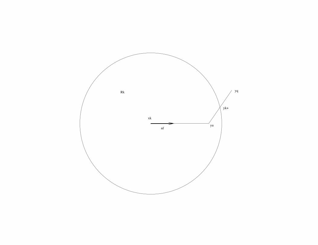
The simplest and most interesting version of such a method

works with a polygon consisting of just two line segments, which

reminds some people of the leg of a dog.

The “knee” of this leg is located at the steepest descent min-

imiser yuk = xk − αu

k∇f(xk), where αuk is as in Lecture 6.

In Lecture 6 we saw that unless xk is a stationary point, we have

yuk = xk −

‖∇f(xk)‖2

∇f(xk)TBk∇f(xk)

∇f(xk).

From yuk the dogleg path continues along a straight line segment

to the quasi-Newton minimiser yqnk .

xk

yu

yq

nf

yk+

Rk

xk

Rk

yk+yu

yq

nf

The dogleg path is thus described by

y(τ) =

xk + τ(yuk − xk) for τ ∈ [0,1],

yuk + (1 − τ)(y

qnk − yu

k) for τ ∈ [1,2].(2)

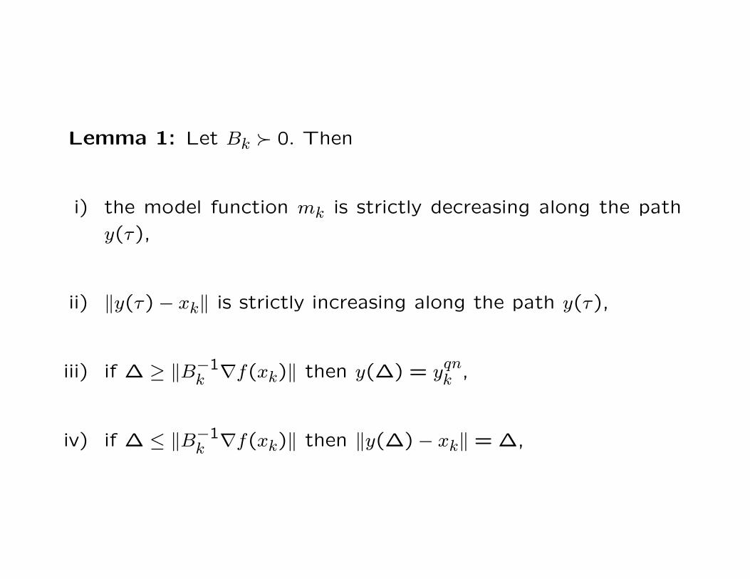
Lemma 1: Let Bk � 0. Then

i) the model function mk is strictly decreasing along the path

y(τ),

ii) ‖y(τ) − xk‖ is strictly increasing along the path y(τ),

iii) if ∆ ≥ ‖B−1k ∇f(xk)‖ then y(∆) = y

qnk ,

iv) if ∆ ≤ ‖B−1k ∇f(xk)‖ then ‖y(∆) − xk‖ = ∆,

v) the two paths x(∆) and y(τ) have first order contact at xk,

that is, the derivatives at ∆ = 0 are co-linear:

lim∆→0+

x(∆) − xk

∆= −

∇f(xk)

‖∇f(xk)‖∼

−‖∇f(xk)‖2

∇f(xk)TBk∇f(xk)

∇f(xk)

= limτ→0+

y(τ) − y(0)

τ.

Proof: See Problem Set 4.

Parts i) and ii) of the Lemma show that the dogleg minimiser

yk+1 is easy to compute:

• If yqnk ∈ Rk then yk+1 = y

qnk .

• Otherwise yk+1 is the unique intersection point of the dogleg

path with the trust-region boundary ∂Rk.

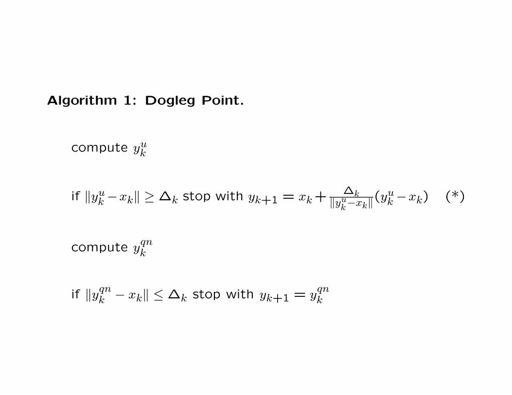
Algorithm 1: Dogleg Point.

compute yuk

if ‖yuk −xk‖ ≥ ∆k stop with yk+1 = xk +

∆k‖yu

k−xk‖

(yuk −xk) (*)

compute yqnk

if ‖yqnk − xk‖ ≤ ∆k stop with yk+1 = y

qnk

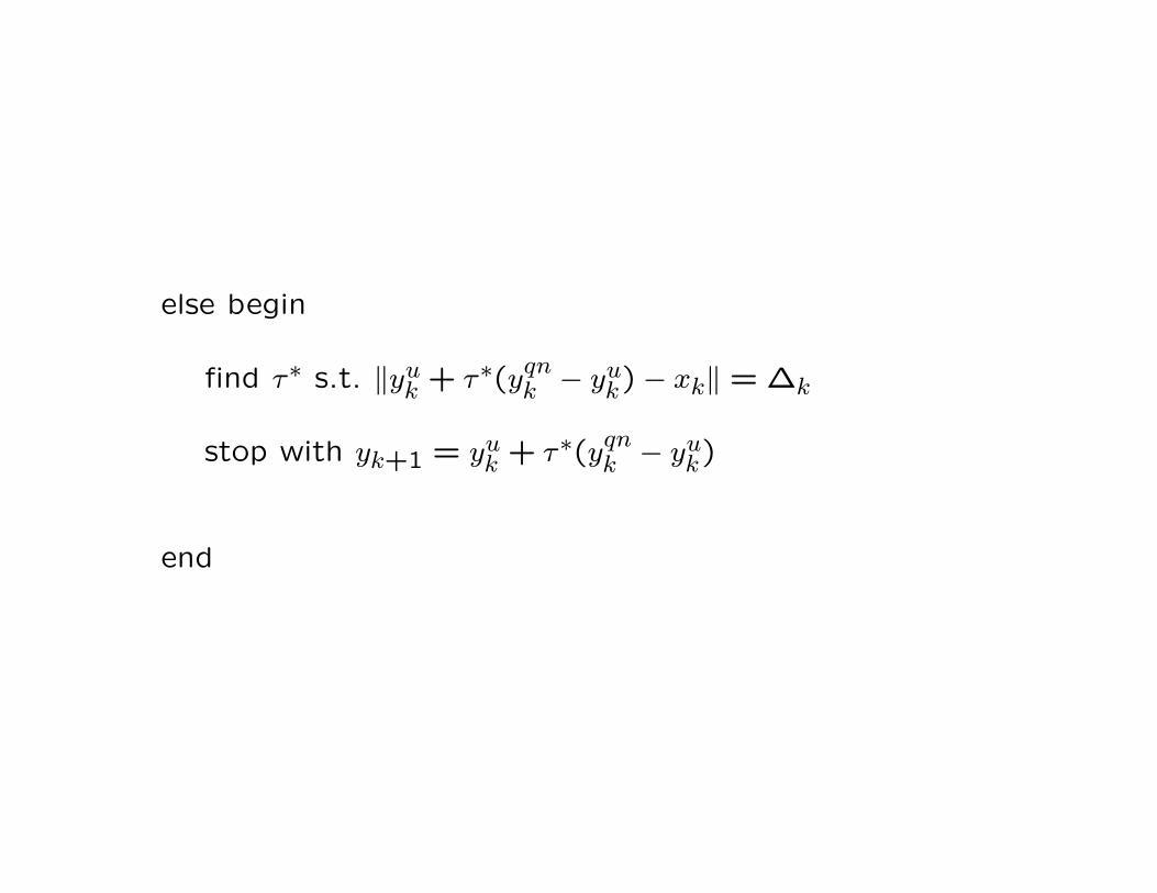
else begin

find τ∗ s.t. ‖yuk + τ∗(y

qnk − yu

k) − xk‖ = ∆k

stop with yk+1 = yuk + τ∗(y

qnk − yu

k)

end

Comments:

• If the algorithm stops in (*) then the dogleg minimiser lies

on the first part of the leg and equals the Cauchy point.

• Otherwise the dogleg minimiser lies on the second part of

the leg and is better than the Cauchy point.

• Therefore, we have mk(yk+1) ≤ mk(yck) as required for the

convergence theorem of Lecture 6.

Steihaug’s Method:

This is the most widely used method for the approximate solution

of the trust-region subproblem.

The method works for quadratic models mk defined by an ar-

bitrary symmetric Bk. Positive definiteness is therefore not re-

quired and SR1 updates can be used for Bk.

It has all the good properties of the dogleg method and more

. . .

Idea:

• Draw the polygon traced by the iterates xk = z0, z1, . . . , zj, . . .

obtained by applying the conjugate gradient algorithm to the

minimisation of the quadratic function mk(x) for as long as

the updates are defined, i.e., as long as dTj Bkdj > 0.

• This terminates in the quasi-Newton point zn = yqnk , unless

dTj Bkdj ≤ 0. In the second case, continue to draw the poly-

gon from zj to infinity along dj, as mk can be pushed to −∞

along that path.

• Minimise mk along this polygon and select yk+1 as the min-

imiser.

The polygon is constructed so that mk(z) decreases along its

path, while Theorem 1 below shows that ‖z − xk‖ increases.

Therefore, if the polygon ends at zn ∈ Rk then yk+1 = zn, and

otherwise yk+1 is the unique point where the polygon crosses

the boundary ∂Rk of the trust region.

Stated more formally, Steighaug’s method proceeds as follows,

where we made use of the identity ∇mk(xk) = ∇f(xk):

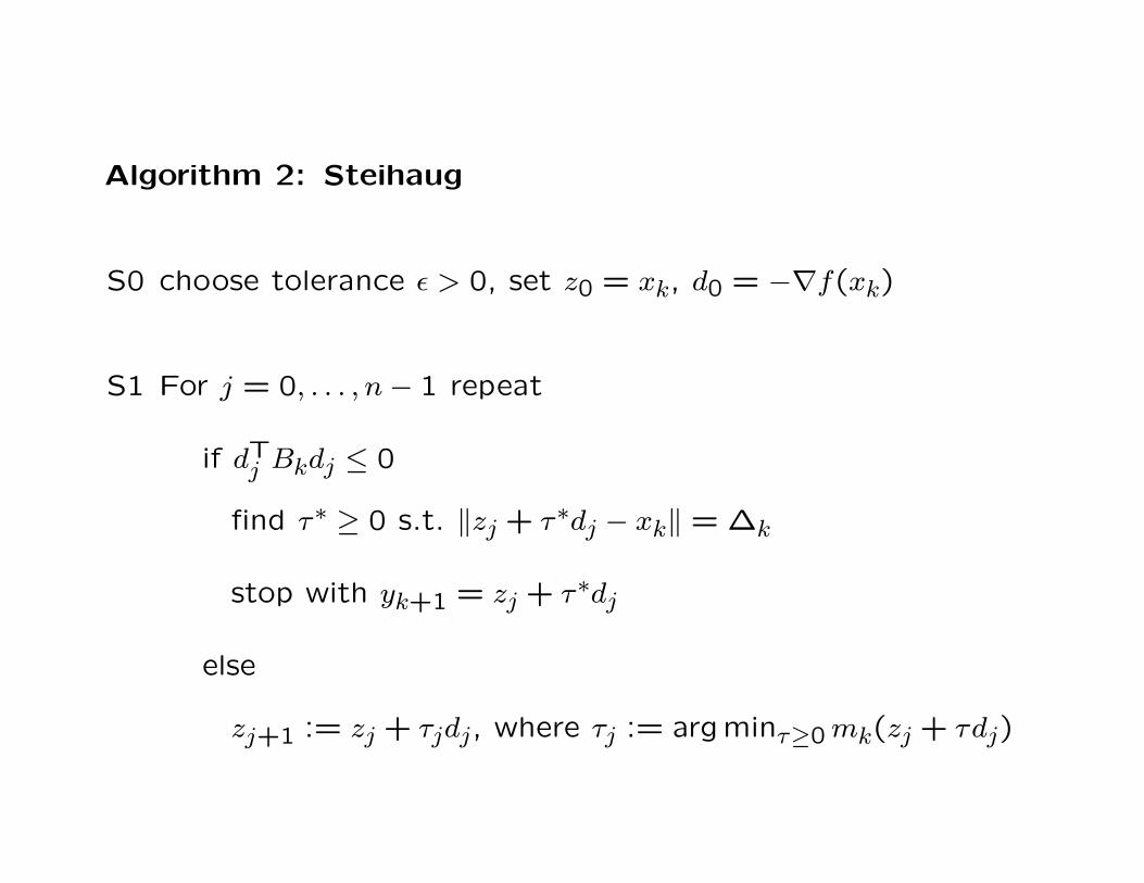
Algorithm 2: Steihaug

S0 choose tolerance ε > 0, set z0 = xk, d0 = −∇f(xk)

S1 For j = 0, . . . , n − 1 repeat

if dTj Bkdj ≤ 0

find τ∗ ≥ 0 s.t. ‖zj + τ∗dj − xk‖ = ∆k

stop with yk+1 = zj + τ∗dj

else

zj+1 := zj + τjdj, where τj := argminτ≥0 mk(zj + τdj)

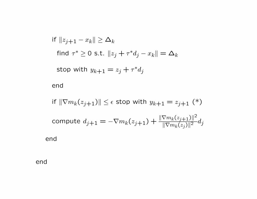
if ‖zj+1 − xk‖ ≥ ∆k

find τ∗ ≥ 0 s.t. ‖zj + τ∗dj − xk‖ = ∆k

stop with yk+1 = zj + τ∗dj

end

if ‖∇mk(zj+1)‖ ≤ ε stop with yk+1 = zj+1 (*)

compute dj+1 = −∇mk(zj+1) +‖∇mk(zj+1)‖

2

‖∇mk(zj)‖2dj

end

end

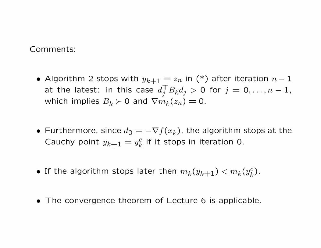
Comments:

• Algorithm 2 stops with yk+1 = zn in (*) after iteration n− 1

at the latest: in this case dTj Bkdj > 0 for j = 0, . . . , n − 1,

which implies Bk � 0 and ∇mk(zn) = 0.

• Furthermore, since d0 = −∇f(xk), the algorithm stops at the

Cauchy point yk+1 = yck if it stops in iteration 0.

• If the algorithm stops later then mk(yk+1) < mk(yck).

• The convergence theorem of Lecture 6 is applicable.

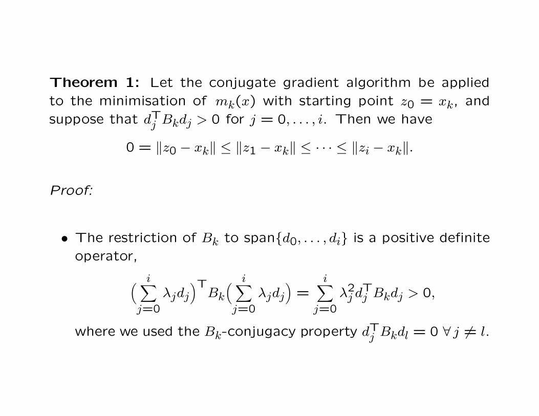
Theorem 1: Let the conjugate gradient algorithm be applied

to the minimisation of mk(x) with starting point z0 = xk, and

suppose that dTj Bkdj > 0 for j = 0, . . . , i. Then we have

0 = ‖z0 − xk‖ ≤ ‖z1 − xk‖ ≤ · · · ≤ ‖zi − xk‖.

Proof:

• The restriction of Bk to span{d0, . . . , di} is a positive definite

operator,

(

i∑

j=0

λjdj

)TBk

(

i∑

j=0

λjdj

)

=i

∑

j=0

λ2j dT

j Bkdj > 0,

where we used the Bk-conjugacy property dTj Bkdl = 0 ∀ j 6= l.

• Therefore, up to iteration i all the properties we derived for

the conjugate gradient algorithm remain valid.

• Since zj − xk =∑j−1

l=0 τldl for (j = 1, . . . , i), we have

‖zj+1 − xk‖2 = ‖zj − xk‖

2 +j−1∑

l=0

τjτldTj dl.

Moreover, τj > 0 for all j.

• Therefore, it suffices to show that dTj dl > 0 for all l ≤ j.

• For j = 0 this is trivially true. We can thus assume that the

claim holds for j − 1 and proceed by induction.

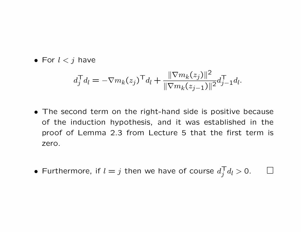
• For l < j have

dTj dl = −∇mk(zj)

Tdl +‖∇mk(zj)‖

2

‖∇mk(zj−1)‖2dTj−1dl.

• The second term on the right-hand side is positive because

of the induction hypothesis, and it was established in the

proof of Lemma 2.3 from Lecture 5 that the first term is

zero.

• Furthermore, if l = j then we have of course dTj dl > 0.

Reading Assignment: Lecture-Note 7.