THE DISTRIBUTED SYSTEMS GROUP, Computer … COLLEGE DUBLIN Management Science and Information Systems Studies Project Report THE DISTRIBUTED SYSTEMS GROUP, Computer Science Department,

TRINITY COLLEGE DUBLIN Management Science and Information Systems Studies Project Report

THE DISTRIBUTED SYSTEMS GROUP, Computer Science Department, TCD.

Analysis of an On-line Random Number Generator

April 2001

Prepared by: Louise Foley Supervisor: Simon Wilson

ABSTRACT The aim of this project was to conduct research of statistical tests for randomness. A collection of recommended tests were made to replace the existing testing program at Random.org. Five tests were chosen on the basis that they were suitable, straightforward and in accordance with the Client’s needs. The implementation and interpretation of each test is defined in this report. These tests are currently being implemented by a final year Computer Science student to run daily on the numbers generated by Random.org. The tests and results will be displayed on the website.

PREFACE The Client for this project was the Distributed Systems Group (DSG) based in Trinity College Dublin. My contact within the DSG was Mr. Mads Haahr, Random.org’s creator. The DSG wanted to replace the existing testing program with a new set of tests. The aim of my project was to present the DSG with a set of recommended tests for their on-line random number generator. In addition to this, I had to provide detailed explanations of implementation and interpretation for each test so that Antonio Arauzo, a final year Computer Science student, could implement the tests for regular use. This report presents the five tests chosen for Random.org. Sample experiments were carried out for four of the tests. The Binary Rank Test proved too difficult to provide an example. This was the main problem I encountered during this project. However, full implementation of this test by Antonio will be possible. Acknowledgements I would like to take this opportunity to say a few thank-yous to the people who helped make this project a success. Firstly, I would like to express my sincere thanks to Mr. Mads Haahr, the designer of Random.org, for all his help and encouragement during this project. I’d especially like to thank him for giving me the opportunity to carry out research into a topic that has always interested me. I would also like to thank Antonio Arauzo for helping me understand the implications of the regular implementation of statistical tests. Finally, my sincerest thanks go to Dr. Simon Wilson who was always ready to help and guide me during the project. He always came up with the most reasonable solutions to my most unreasonable queries.

“It is impossible to tell if a single number is random or not. Random is a negative property; it is the absence of order”

David Ceperley Dept. of Physics

University of Illinois

THE DISTRIBUTED SYSTEMS GROUP Analysis of an Online Random Number Generator 9th April 2001

TABLE OF CONTENTS NO. SECTION PAGE 1 INTRODUCTION AND SUMMARY 1 1.1 The Client 1 1.2 The Project Objective 1 1.3 Terms of Reference 2 1.4 Report Summary 2 2 CONCLUSIONS AND RECOMMENDATIONS 3 3 EXPLORATORY DATA ANALYSIS 5 3.1 The Objective of Exploratory Data Analysis 5 3.2 Summary Statistics 5 3.3 Data Analysis Plots 5 4 THE TEST CRITERIA AND THE TESTS CHOSEN 9 4.1 The Test Criteria 9 4.2 The Theoretical Tests 10 4.3 The Empirical Tests 12 5 RESULTS ON RANDOM.ORG 13 5.1 Choice of Sample Size for the Test 13 5.2 The Results of the Tests 13 6 COMPARISON TO OTHER GENERATORS 19 6.1 Comparison of Generators 19

APPENDICES

NO. CONTENT PAGE A. Original Project Outline A.1 B. Interim Report B.1 C. Technical Commentary C.1 D. Background to Random Numbers D.1 E. How the Numbers were Generated E.1 F. Exploratory Data Analysis on Lavarand.sgi.com and L’Ecuyer’s PRNG F.1 G. Descriptions of the Tests Used G.1 H. Hypothesis Testing H.1 I. Statistical Tables I.1 J. Statistical Tests Reviewed for Analysis J.1 K. Glossary K.1 REFERENCES

DSG – Analysis of an Online RNG 1 April 2001 ____________________________________________________________________________________________________

1. INTRODUCTION AND SUMMARY This chapter introduces the client and the project, including the terms of reference. It also gives a short overview of the remaining chapters.

1.1 The Client The Distributed Systems Group (DSG) [9] is a research group run by members of the Computer Science Department in Trinity College. DSG conducts research into all areas of distributed computing including, amongst others, parallel processing in workstation clusters, support for distributed virtual enterprises and mobile computing. The website www.random.org which provides the random numbers is hosted by DSG. It was set up in October 1998 by Mads Haahr to provide easily accessible random numbers to the general public over the Internet. It is currently one of three online true random number generators. The generator uses atmospheric noise to produce strings of random bits. These numbers are available free of charge on the website. The site currently uses John Walker’s ENT program to test the numbers generated. Walker is based in Fourmilab in Switzerland. Fourmilab runs one of the other online true random number generators, www.fourmilab.ch/hotbits. The ENT program is also used to analyse the numbers generated by the Hotbits generator.

1.2 The Project Objective The objective of this project is to recommend a new set of tests that can be used to replace the ENT program to analyse the generator and the numbers it produces. The test results given in Section 5.2 are mainly for illustrative purposes. The tests were run to show the steps involved in each test and to aid interpretation of the results of the tests. Thus, as the sample size is quite small the results don’t hold much statistical weight. They are, however, appropriate for explaining the tests chosen.

http://www.random.org/

http://www.fourmilab.ch/hotbits


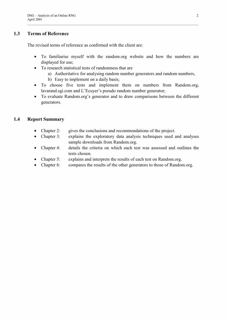
1.3 Terms of Reference The revised terms of reference as confirmed with the client are:

• To familiarise myself with the random.org website and how the numbers are displayed for use;

• To research statistical tests of randomness that are a) Authoritative for analysing random number generators and random numbers, b) Easy to implement on a daily basis;

• To choose five tests and implement them on numbers from Random.org, lavarand.sgi.com and L’Ecuyer’s pseudo random number generator;

• To evaluate Random.org’s generator and to draw comparisons between the different generators.

1.4 Report Summary

• Chapter 2: gives the conclusions and recommendations of the project. • Chapter 3: explains the exploratory data analysis techniques used and analyses

sample downloads from Random.org. • Chapter 4: details the criteria on which each test was assessed and outlines the

tests chosen. • Chapter 5: explains and interprets the results of each test on Random.org. • Chapter 6: compares the results of the other generators to those of Random.org.


2. CONCLUSIONS AND RECOMMENDATIONS The properties of random numbers are presented in Appendix D.3, p. D.2, and are referred to throughout the report. The exploratory data analysis section (chapter 3, p. 5) shows that the numbers meet each of these properties. Uniformity is confirmed by the histogram and the chi-squared tests. The autocorrelation plot illustrates the property of independence. The properties of summation and duplication are satisfied by the results of the summary statistics (section 3.2, p.5). Exploratory data analysis is a very important part of any statistical analysis and I therefore recommend that the Client investigate the possibility of including some graphical EDA and/or statistical summaries. They can convey useful, uncomplicated information about the numbers and the generation process. Section 4.1, p. 9, gives the criteria for choosing tests for this project. These are:

• The complete set of tests will comprise of a mix of both theoretical and empirical tests;

• Each test will highlight something different; • The tests will be suitable for the purpose of analysing random numbers and random

number generators; • The tests will be easy to implement for daily use so that they can be run on samples of

numbers generated daily on Random.org. These test results will be available on the site for users to check the performance of the Random.org generator.

The five tests chosen are:

• A chi-squared test; • A test of runs above and below the median; • A reverse arrangements test; • An overlapping sums test; • A binary rank test for 32x32 matrices.

All of the chosen tests meet the above criteria. This makes them the most suitable collection of tests for analysing the generator. I recommend that the Client implement all of them to run daily (or at regular time intervals) on numbers generated by Random.org. However, if it is not possible to implement the Binary Ranks Test fully, I still recommend implementing the remaining four tests. Section 5.1, p. 13, presents the reasons for the choice of a sample size of 10,000. Section 5.2, p. 13, deals with the formal hypothesis results of the tests and the results for Random.org. The generator passed all the sample tests. A detailed description of hypothesis testing is given in Appendix H, p. H.1, and the relevant statistical tables are reproduced in

DSG – Analysis of an Online RNG 4 April 2001 ____________________________________________________________________________________________________ Appendix I, p. I.1. I recommend that Random.org place copies of these tables and hypothesis layout on the website for the users use in interpreting the tests and the results. Section 6.1, p. 20, compares Random.org, Lavarand.sgi.com and L’Ecuyer’s PRNG (pseudo random number generator) on the basis of performance and speed; and Random.org and Lavarand.sgi.com on the basis of website layout. Overall I found that Random.org does very well on all three factors, but I recommend a better use of colour and graphics to improve the aesthetic quality of the site.


3. EXPLORATORY DATA ANALYSIS ON RANDOM.ORG This chapter gives the results of the exploratory data analysis on 1,000 numbers generated by Random.org. It gives summary statistics and data analysis plots for the numbers. The results of exploratory data analysis on numbers generated by Lavarand.sgi.com and L’Ecuyer’s PRNG (pseudo random number generator) are reproduced in Appendix F, p. F.1.

3.1 The Objective of Exploratory Data Analysis The objective of exploratory data analysis (EDA) is to become familiar with the data. It is always necessary to conduct exploratory data analysis on a data set before more formal tests are applied. EDA techniques are usually graphical and they are especially useful, providing a visual exploration of the data. The next two sections deal with two aspects of EDA, summary statistics and data analysis plots.

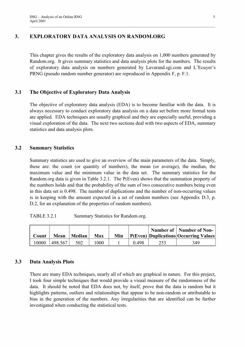
3.2 Summary Statistics Summary statistics are used to give an overview of the main parameters of the data. Simply, these are: the count (or quantity of numbers), the mean (or average), the median, the maximum value and the minimum value in the data set. The summary statistics for the Random.org data is given in Table 3.2.1. The P(Even) shows that the summation property of the numbers holds and that the probability of the sum of two consecutive numbers being even in this data set is 0.498. The number of duplications and the number of non-occurring values is in keeping with the amount expected in a set of random numbers (see Appendix D.3, p. D.2, for an explanation of the properties of random numbers). TABLE 3.2.1 Summary Statistics for Random.org.

Count Mean Median Max Min P(Even) Number of

Duplications Number of Non-

Occurring Values 10000 498.567 502 1000 1 0.498 253 349

3.3 Data Analysis Plots There are many EDA techniques, nearly all of which are graphical in nature. For this project, I took four simple techniques that would provide a visual measure of the randomness of the data. It should be noted that EDA does not, by itself, prove that the data is random but it highlights patterns, outliers and relationships that appear to be non-random or attributable to bias in the generation of the numbers. Any irregularities that are identified can be further investigated when conducting the statistical tests.

DSG – Analysis of an Online RNG 6 April 2001 ____________________________________________________________________________________________________ The four techniques I chose are: • A run sequence plot; • A lag plot; • A histogram; • An autocorrelation plot. The Run Sequence Plot The run sequence plot is a graph of each observation against the order it is in the sequence. The graph below is the run sequence on a set of 1,000 numbers taken from Random.org. This run sequence plot shows a random pattern. The plot fluctuates around 500, the expected (or true) mean of the numbers, and these fluctuations appear random. There are no upward, downward or cyclical trends evident in this graph.

FIGURE 3.3.1 Run Sequence Plot for Random.org. The Lag Plot The lag plot is a scatter plot of each observation against the previous observation. This particular type of graph is very good at detecting outliers. Outliers always need to be examined. If they are just chance outliers then they need to be deleted from the data set before analysis can be carried out. However, if there are many or significant outliers, this is an indication that there may be something wrong with the generator. Figure 3.3.2 shows no outliers and the data points are spread evenly across the whole plain. This is a good indication of randomness.


FIGURE 3.3.2 Lag Plot for Random.org. The Histogram The histogram plots a count of observations that occur in each subgroup. Therefore I expect there to be almost the same number of observations in each category. In Figure 3.3.3 there are 10 categories and approximately 100 observations in each. The histogram confirms the property of uniformity.

FIGURE 3.3.3 Histogram for Random.org. The Autocorrelation Plot Autocorrelation occurs when an observation is, in some part, determined by the preceding observations. This is a very common kind of non-randomness. Before the plot could be drawn, lags were set up. The lag is of one; so the second observation is compared to the first and so on. The autocorrelation plot below (Figure 3.3.4) suggests that the Random.org data is indeed random. All the values are in control (inside the red dotted lines) and all the correlations are small (the absolute values are less than 0.1). This indicates that the numbers hold the property of independence, as there is not much dependence between successive observations (a more complete list of the properties of random numbers can be found in Appendix D.3, p. D.2).


10 20 30

-1.0-0.8-0.6-0.4-0.20.00.20.40.60.81.0

Auto

corre

latio

n

1 2 3 4 5 6 7 8 9

101112131415161718

192021222324252627

282930

0.04-0.07 0.00 0.01 0.03-0.02-0.00-0.00-0.07

-0.02 0.01 0.05-0.03 0.02 0.05-0.04-0.06-0.04

-0.02-0.01-0.02 0.04 0.06 0.03-0.02-0.02 0.02

0.04-0.08-0.02

1.27-2.28 0.03 0.16 0.80-0.78-0.08-0.14-2.16

-0.48 0.41 1.65-1.04 0.71 1.55-1.28-1.94-1.37

-0.69-0.19-0.46 1.14 1.82 0.93-0.52-0.52 0.76

1.11-2.46-0.47

1.61 6.86 6.86 6.89 7.54 8.17 8.18 8.2012.98

13.2113.3816.2317.3617.8920.4322.1526.1628.17

28.6828.7228.9530.3733.9834.9235.2235.5236.16

37.5344.2444.49

Lag Corr T LBQ Lag Corr T LBQ Lag Corr T LBQ Lag Corr T LBQ

Exploratory Data Analysis Autocorrelation Plot

FIGURE 3.3.4 Autocorrelation Plot for Random.org. The exploratory data analysis appears to support the hypothesis that the numbers are random. The summary statistics show that the size of the data set (i.e. the quantity, maximum and minimum values) provides a reasonable basis for assuming that the numbers are random. Furthermore the mean of 498.5 agrees with the property of uniformity, as does the histogram plot. The autocorrelation plot and the low values for correlation validate the property of independence. The run sequence plot and the lag plot do not highlight any outliers or inconsistencies in the data that could influence the results of the tests.


4. THE TEST CRITERIA AND THE TESTS CHOSEN This chapter explains what the criteria were for choosing the tests, which tests were chosen and explains how each met the required criteria. An explanation of each test is given in Appendix G, p. G.1. The results of the hypothesis testing on Random.org are presented in Section 5.2, p. 13. A discussion of hypothesis testing can be found in Appendix H, p.H.1.

4.1 The Test Criteria The objective of the project was to review statistical tests for randomness and choose a number of tests to run on numbers generated by the Random.org generator. In conjunction with the Client, I identified four criteria on which the tests would be chosen. A full list of the tests reviewed can be found in Appendix J, p. J.1. The criteria are as follows:

• The complete set of tests will comprise of a mix of both theoretical and empirical tests. This means that some tests are based on statistical theories and some on evidence inherent in the numbers generated;

• Each test will highlight something different e.g. trends in the data attributed to non-random influences etc.;

• The tests will be suitable for the purpose of analysing random numbers and random number generators;

• The tests will be easy to implement for daily use so that they can be run on samples of numbers generated daily on Random.org. These test results will be available on the site for users to check the performance of the Random.org generator.

The last two criteria are the most important to the Client and tests that incorporated both these conditions were given the highest priority when choosing tests. The five tests chosen were:

• A chi-squared test; • A test of runs above and below the median; • A reverse arrangements test; • An overlapping sums test; • A binary rank test for 32x32 matrices.

These divided into theoretical and empirical tests as show in Table 4.1.1.

DSG – Analysis of an Online RNG 10 April 2001 ____________________________________________________________________________________________________ TABLE 4.1.1 Theoretical and Empirical Tests Theoretical Tests Empirical Tests

The chi-squared test The overlapping sums test

The test of runs above and below the median The binary rank test for 32x32 matrices

The reverse arrangements test

4.2 The Theoretical Tests The Chi-Squared Test According to the properties of random numbers (see Appendix D.3, p. D.2) the numbers should be distributed uniformly. The chi-squared test is a test of distributional accuracy. That is, it measures how closely a given set of numbers follows a particular distribution, namely there uniform distribution. Thus, if a generator passes this test it has satisfied one of the properties of random numbers. The chi-squared test is a very common statistical test and is widely used in the analysis of random numbers. The test is easily understood and often used by non-statistical disciplines and its critical values are easy to understand and interpret. It is very clear when the null hypothesis is accepted and when it is not for a given data set. This test is also very simple to implement for daily use. As this characteristic is very important to the Client, the chi-squared test is included in this project. In order to combine the results of successive experiments made at different times, the calculated values of χ2 and the number of degrees of freedom (df) are added across the different experiments. Then the total value of χ2 is tested with the total number of degrees of freedom. To store a running score only the current value of χ2 and the current number of degrees of freedom needs to be stored. Then each day as a new experiment is conducted the new values of χ2 and degrees of freedom can be added to the current ones. For example, on day one I run a chi-squared test on 1,000 numbers. The current_ χ2 = 5.9901 and the current_df = 9. In this experiment I accept the null hypothesis. On day two I run the test again on another 1,000 numbers. Then the new_ χ2 = 10.6394 and the new_df = 9. To calculate the χ2 value of both test let χ2=current_ χ2+ new_ χ2 = 16.6295. The total df = current_df + new_df = 18. The critical value of a chi-squared test with 18 degrees of freedom is

χ =218,05.0 28.87

⇒ accept the null hypothesis. Note: In the above example both the individual experiment values are not significant as is the aggregated value. However, it should be noted that the aggregated value might be significant even though some of the individual experiment values are not significant. All the same, if too

DSG – Analysis of an Online RNG 11 April 2001 ____________________________________________________________________________________________________ many experiments are added together then ultimately the test sample will become too big and a significant result could be returned even if the null hypothesis is true (In statistics this is called a Type 1 error). The Test of Runs Above and Below the Median The runs test is a common, non-parametric, distribution-free test. This means that no assumptions are made about the population distribution’s parameters (mean, standard deviation etc.) It was chosen specifically as it is very powerful in detecting fluctuating trends in the data. Existence of such trends would suggest non-randomness. The test checks for trends by examining the order in which the numbers are generated. If the numbers are not generated in a random order, then this may indicate a gradual bias in the software that generates the numbers. The existence of such a bias would need to be addressed by the Client (see Section 5.2, p. 13). Following the exploratory data analysis stage non-random patterns may be identified in the data. The test of runs above and below the mean is very useful to check if these patterns are attributable to non-randomness (and not to chance). Observations in a sequence of numbers greater than the median of the sequence are assigned the letter “a” and observations less that the median are assigned the letter “b”. Observations equal to the median are omitted. Then u, the total number of runs, n1, the number of a’s and n2, the number of b’s are calculated. The test is especially powerful in detecting trends and cyclical patterns. If the sequence contains mostly b’s at first and then mostly a’s this indicates an upward trend in the data. The opposite is true for a downward trend where a’s will occur more frequently at the beginning of the sequence giving way to mostly b’s later in the sequence. Cyclical patterns are characterised by constantly alternating sequences of a’s and b’s and usually too many runs. The runs test, too, is very easy to implement on a daily basis. Once the test is run on one set of numbers the values for u, n1 and n2 are stored. When the test is run on a new set of numbers the new values of u, n1 and n2 are added to the stored values. Then the mean, µu, and the standard deviation, σu, are calculated. Finally, the z-score for the combined test is calculated. The Reverse Arrangements Test Another test that is also powerful in detecting bias in the software used is the reverse arrangements test. This test is particularly good at detecting monotonic (i.e. gradual and continuing) trends in the data. The existence of these trends also indicates non-randomness. The test was developed by Bendat and Peirsol [3] and is a well-known and accurate test of randomness.

DSG – Analysis of an Online RNG 12 April 2001 ____________________________________________________________________________________________________ The test can quite successfully be used daily to keep a running score. After the test is run store the value for A. Then on day two add the value of new_A to A and consult the table for the critical values. An average for A can be computed so that the table of critical values may be used. The table of values can be found in Appendix I.3, p. I.3.

4.3 The Empirical Tests The Overlapping Sums Test and The Binary Rank Test for 32x32 Matrices The empirical tests are taken from a collection devised by George Marsaglia called the Diehard Suite. Marsaglia has spent over 40 years working in the field of random numbers and random number generators. The Diehard Suite of tests is widely regarded as a very comprehensive collection of tests for randomness. This is why I chose to recommend two of Dr. Marsaglia’s empirical tests from the Diehard Suite. These tests are a little more difficult to implement on a daily basis. Both tests finish with a chi-squared test so summaries of previous χ2 values can be computed and maintained as explained above in Section 4.2, p 10. Even though there are difficulties associated with implementing these tests on a daily basis, I felt these tests needed to be included in the analysis. Firstly, because as mentioned above they are part of Marsaglia’s Diehard Suite. Secondly, because they are empirically based tests. Thirdly, because the Diehard tests are designed to measure the performance of random number generators as well as sequences of random numbers. The binary rank test was chosen in particular because it uses bits to test the generator. This was very important because the binary download option on Random.org is the second most common form that is used by users to generate random numbers. I felt it was necessary to analysis this option too.


5. RESULTS ON RANDOM.ORG This chapter explains how the results of each test were interpreted. It also gives an explanation of the sample size chosen.

5.1 Choice of Sample Size for the Test

The five tests were run on numbers downloaded from the Random.org website. This sample is used to show how the chosen tests would work. The tests will eventually be implemented to be carried out on a daily basis on a sample of numbers from the generator. In this project the tests are carried out mainly for illustrative purposes (see Section 1.2, p. 1). However, some conclusions can be drawn from the analysis presented below. I downloaded a set of 10,000 numbers from the Random.org website. The first four tests were performed on these numbers or a sub-sample of these numbers. For the binary rank test I downloaded a separate file of 1,099,860 random bits. All 10,000 numbers were used for the chi-squared and the runs test. However, because of the restrictions involved with the reverse arrangements test and the overlapping sums test, only 500 numbers were used in running these tests (see Appendices G.3, p. G.3, and G.4, p. G.5). Obviously a complete computer program can easily run these tests on larger sets of numbers.

5.2 The Results of the Tests The numbers generated by Random.org passed all of my chosen tests. This indicates that it is producing “good” random numbers. The Client feels that this is very important because if my research showed some flaw in the generation of the numbers, he felt that the software and the generation process would need to be reviewed. After carrying out my research I do not believe that such a review is necessary. I believe based on the results given below that Random.org runs a very good random number generator. The Chi-Squared Test Table 5.2.1 below gives the observed and expected frequencies for the chi-squared test on the 10,000 numbers. The deviations from the expected values are easily seen in Figure 5.2.1.

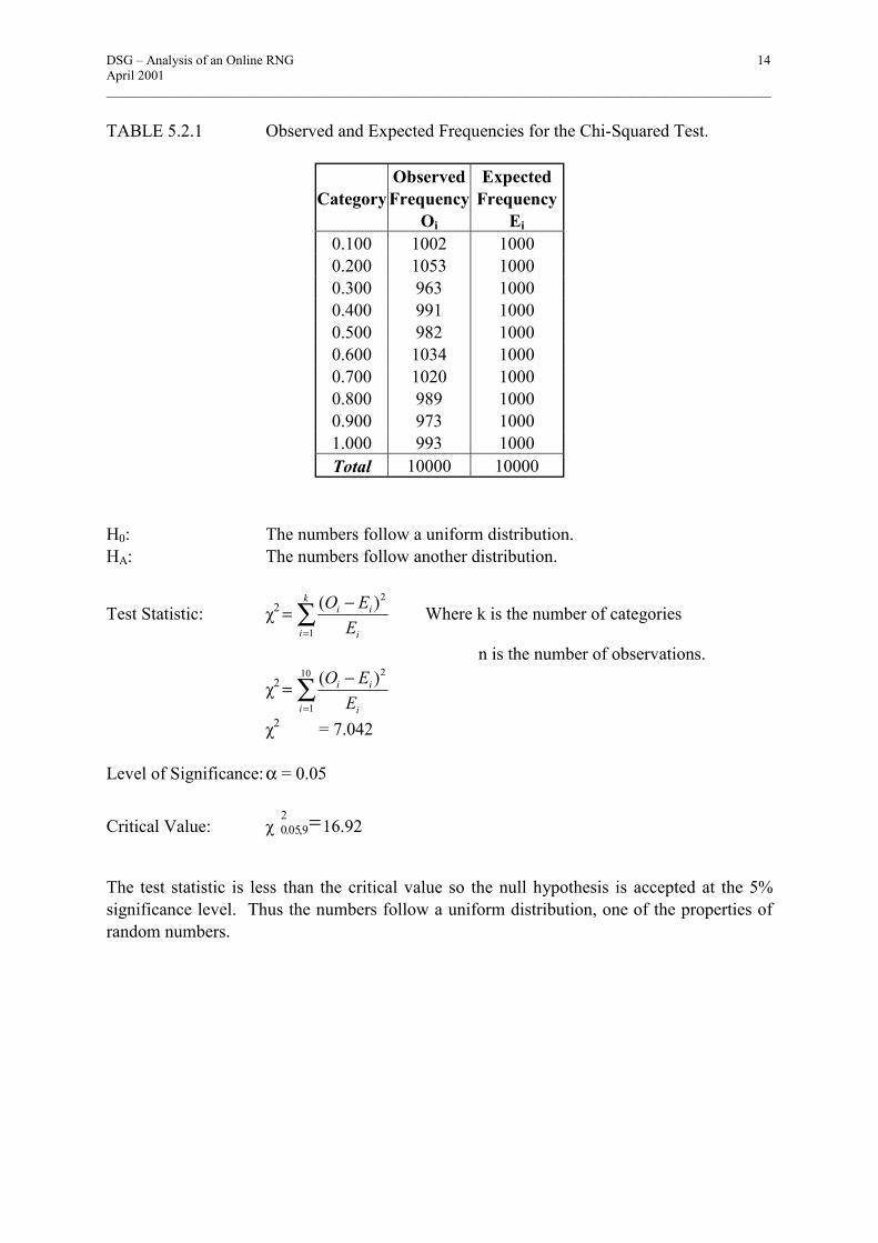
DSG – Analysis of an Online RNG 14 April 2001 ____________________________________________________________________________________________________ TABLE 5.2.1 Observed and Expected Frequencies for the Chi-Squared Test.

Category

Observed Frequency

Oi

Expected Frequency

Ei 0.100 1002 1000 0.200 1053 1000 0.300 963 1000 0.400 991 1000 0.500 982 1000 0.600 1034 1000 0.700 1020 1000 0.800 989 1000 0.900 973 1000 1.000 993 1000 Total 10000 10000

H0: The numbers follow a uniform distribution. HA: The numbers follow another distribution.

Test Statistic: χ2 ∑=

−=k

i i

ii

EEO

1

2)( Where k is the number of categories

n is the number of observations.

χ2 ∑=

−=10

1

2)(i i

ii

EEO

χ2 = 7.042 Level of Significance: α = 0.05

Critical Value: χ =29,05.0 16.92

The test statistic is less than the critical value so the null hypothesis is accepted at the 5% significance level. Thus the numbers follow a uniform distribution, one of the properties of random numbers.


Frequency Histogram

0

200

400

600

800

1000

1200

0.1 0.2 0.3 0.4 0.5 0.6 0.7 0.8 0.9 1.0

Category

Freq

uenc

y

Observed Frequency Expected Frequency

FIGURE 5.2.1 Bar Chart of Expected and Observed Frequencies. The Test of Runs Above and Below the Median TABLE 5.2.2 Summary Statistics for the Runs Test

u n1 n2 µµµµu σσσσu z 4979 4995 4995 4996 49.9725 -0.3502

H0: The numbers are generated in a random order. HA: The numbers are not generated in a random order.

Test Statistic: u

uuzσ

µ−±= )5.0( Where µu is the mean of the distribution of u.

σu is the standard deviation of u.

97.49

4996)5.04979( −±=z

z = -0.3502

Level of Significance: α = 0.05 Critical Value: |z| < zα/2

-z -α/2 < -0.3502 < z α/2 ⇒ -z –0.025 < -0.3502 < z 0.025

-1.96 < -0.3502 < +1.96

DSG – Analysis of an Online RNG 16 April 2001 ____________________________________________________________________________________________________ As the current value for z lies between ±1.96 then the null hypothesis is accepted at the 5% significant level. Therefore there is no evidence to suggest a bias in the generator’s software. The result of this test confirms that the random patterns identified in the EDA stage are attributable to randomness. The Reverse Arrangements Test H0: The numbers generated do not exhibit monotonic trends. HA: The numbers generated exhibit monotonic trends.

Test Statistic: ∑ ∑−

= +=

=

1

1 1

N

j

N

ijijhA

1 if xi > xj Where hij =

0 else N is the number of observations.

∑ ∑= +=

=

99

1

100

1j ijijhA

A = 2536 Level of Significance: α = 0.05 Critical Value: AN:(1-α/2) < 2536 ≤ AN;( α/2) A100;0.975 < 2536 ≤ A100;0.025 ⇒ 2145 < 2536 ≤ 2804 As the value for A in this experiment lies between 2145 and 2804 then the null hypothesis is accepted at the 5% significance level. Table 5.2.3 below shows the results for each of the five individual experiments and also the averaged value of A over the five tests. The average value is not significant and neither are any of the individual tests. TABLE 5.2.3 Test Values for the Five Experiments in the Reverse Arrangements Test

A_1 A_2 A_3 A_4 A_5 AvgA 2536 2453 2502 2588 2400 2496

There is no evidence to say that the data has monotonic trends. This supports the result of the test for runs (p 16) and the assumption that there is no evidence to suggest bias in the generator’s software.

DSG – Analysis of an Online RNG 17 April 2001 ____________________________________________________________________________________________________ The Overlapping Sums Test As described in Appendix G.4, p. G.5, the overlapping sums minus the means are pre-multiplied by matrix A and then converted to uniform variables. A chi-squared test is then carried out on the numbers. Table 5.2.4 gives the observed and expected frequencies for this chi-squared test on the 500 numbers is given below. The deviations from the expected values are easily seen in Figure 5.2.2. TABLE 5.2.4 Observed and Expected Frequencies for the Chi-Squared Test.

Category Observed Frequency

Oi

Expected Frequency

Ei 0.100 43 50 0.200 58 50 0.300 49 50 0.400 53 50 0.500 43 50 0.600 55 50 0.700 47 50 0.800 63 50 0.900 46 50 1.000 43 50 Total 500 500

H0: The numbers follow a uniform distribution HA: The numbers follow another distribution

Test Statistic: χ2 ∑=

−=k

i i

ii

EEO

1

2)( Where k is the number of categories

n is the number of observations.

χ2 ∑=

−=10

1

2)(i i

ii

EEO

χ2 = 8.8 Level of Significance: α = 0.05

Critical Value: χ =29,05.0 16.92

The test statistic is less than the critical value so the null hypothesis is accepted at the 5% significance level. The resulting numbers fit a uniform distribution and the generator passes this test.


Frequency Histogram

0

25

50

0.1 0.2 0.3 0.4 0.5 0.6 0.7 0.8 0.9 1.0

Category

Freq

uenc

y

Observed Frequency Expected Frequency

FIGURE 5.2.2 Bar Chart of Expected and Observed Frequencies The Binary Rank Test for 32x32 Matrices I was unable to obtain sample results for this test, as mentioned in Section 5.1, p. 13. Originally I downloaded 1,099,860 bits from Random.org. When I ran the "Rankstes" program (see Appendix G.5, p. G.5) the results were inconclusive. The test is supposed to be run on 40,000 matrices. The data set only produced 1,074 matrices. It is consequently not possible to provide an example of this tests in this report. However, I believe this is an appropriate test to include. If the test can be implemented to run on 40,000 matrices, I recommend that the Client adopt this test. When the ranks of the matrices are found a chi-squared test should be performed. The expected frequencies for this chi-squared test are given in Table 5.2.4 below. TABLE 5.2.4 Expected Value for the Ranks Test Chi-Squared Test

Rank Expected % <29 211.5 0.529 30 5134 12.835 31 23103 57.758 32 11551.5 28.879 40000 100.000

Equally so the test could not be run on the Lavarand.sgi.com generator or L’Ecuyer’s PRNG. Thus this test is not included in the comparison of the generators in the next chapter (see section 6.1, p.20).


6. COMPARISON TO OTHER GENERATORS This chapter provides the results found for the tests on the other two generators, Lavarand.sgi.com’s true random number generator and L’Ecuyer’s PRNG (pseudo random number generator). A description of these generators is found in Appendix E.

6.1 Comparison of Generators When comparing the Random.org generator to the Lavarand.sgi.com generator and L’Ecuyer’s PRNG three decisive factors were taken into consideration.

• Performance; • Speed; • Website layout (although this does not apply to the PRNG).

Performance TABLE 6.1.1 Comparison of Results on Random.org, Lavarand.sgi.com and L’Ecuyer’s PRNG.

Test Statistics

Test Critical Values Random.org Lavarand.sgi.com L’Ecuyer’s

PRNG The Chi-Squared

Test χ =2

9,05.0 16.92 χ2 = 7.04 χ2 = 5.91 χ2 = 11.86

Accept Ho Accept Ho Accept Ho The Test of Runs Above and Below

the Median |z| < 2 z = -0.3502 z = -0.4302 z = -0.5799

Accept Ho Accept Ho Accept Ho The Reverse

Arrangements Test

2145<A≤2804 A = 2496 A = 2500 A = 2565

Accept Ho Accept Ho Accept Ho The Overlapping

Sums Test χ =2

9,05.0 16.92 χ2 = 8.8 Χ2 = 7.08 χ2 = 4.48

Accept Ho Accept Ho Accept Ho There is not enough evidence to say that any of the generators failed any of the tests. The results of each test are reproduced in Table 6.1.1. While the generators all got different results there is no method in statistics for saying that one “in control” result is “better” than the next.

DSG – Analysis of an Online RNG 20 April 2001 ____________________________________________________________________________________________________ Statistically, Random.org is just as good a generator as the other two. The numbers do pass the tests. If the tests had given drastically different results for each generator then it would have indicated that at least one of them was not a good generator [2]. Speed L’Ecuyer’s PRNG is the fastest generator; PRNG’s usually are compared to true RNG’s. Also, on both Random.org and Lavarand.sgi.com there is a maximum amount of numbers that can be downloaded each time. Thus when a lot of numbers are required then several downloads must be made from both Random.org and Lavarand.sgi.com. However, L’Ecuyer’s PRNG can produce a much larger amount of numbers each time it is run. Lavarand.sgi.com is slightly quicker than Random.org because the page is updated every minute. So, the user needs to wait only one minute for the next block of data. If a large set is required from Random.org then the user may have to wait a few minutes. Website Layout While this characteristic obviously does not apply to L’Ecuyer’s PRNG, it is nonetheless a very important criterion on which the Random.org site should be evaluated. If the site were very complicated, boring or difficult to access then the Client would have to review this. The numbers can be obtained very easily from Random.org’s website. This makes up for it’s slightly slower generation time. They come formatted in columns and the user can specify how many columns they would like and the maximum and minimum values of the numbers generated. This makes it very easy for the user to get exactly what they want. Lavarand.sgi.com, on the other hand, with their animated flashing lava lamps, have a more information-orientated site. There is no direct link from the homepage to the generated numbers. Also, and more importantly, the user cannot specify minimum and maximum values or the length of the data required etc. Lavarand.sgi.com produces a 4096-byte block every minute and update the web page with each new block. Users then have to copy the block and format it themselves. Random.org passes the four sample tests; it is also reasonable fast compared to the other generators; and presents its generated numbers in the most accessible form.

Page A.1

A. ORIGINAL PROJECT OUTLINE MSISS Project Outline – 2000/01 Client: Distributed Systems Group, Computer Science Dept., Trinity College Project: “On-line statistical analysis of a true random number generator” Location: College Contact: Mads Haahr, [email protected], phone (01) 608 1543 Dept Contact Simon Wilson The Distributed Systems Group (http://www.dsg.cs.tcd.ie/) is operating a public true random number service (http://www.random.org/) that generates true randomness based on atmospheric noise. The numbers are currently made available via a web server. Since it went online in October 1998, random.org has served nearly 10 billion random bits to a variety of users. Its popularity is currently on the rise and at the moment the web site receives approximately 1,000 hits per day. The objectives of this project are first to implement a suite of statistical tests for randomness on the output stream. These are to be implemented using a statistical package, Excel or, if the student wants, by writing code. Then, a comparison should be made with other ‘true’ random number generators and with some of the more usual ‘pseudo’ random generation algorithms. The second part of the project involves integrating the test functionality with the random.org number generator. This may involve managing a database containing the numbers generated (or, possibly, a summary of the numbers) and linking an analysis of the database to the web for users of the service. Clearly the first part of this project is overwhelmingly statistical in nature. A survey of suitable statistical tests will have to be made, and then the tests implemented, using a statistical package, Excel or through writing code explicitly. The second part of the project involves managing a database (the numbers generated) and linking an analysis of the database to the web for users of the service.

mailto:[email protected]

http://www.dsg.cs.tcd.ie/


Page B 1

B. INTERIM REPORT

Management Science and Information Systems Studies Project: Analysis of On-line True Random Number Generator Client: Distributed Systems Group, Computer Science Dept., Trinity College Student: Louise Foley Supervisor: Simon Wilson Review of Background and Work to Date The Distributed Systems Group (DSG) is a research group run by members of the Computer Science Dept in Trinity College. Research within the Group covers all aspects of distributed computing ranging from parallel processing in workstation clusters through support for distributed virtual enterprises to mobile computing. The objective of my project is to analyse their on-line random number generator. The generator uses atmospheric noise to produce strings or true random numbers on their website www.random.org. To date the work I’ve done is summarised as follows.

• I visited both the DSG website and the Random.org website to familiarise myself with the service.

• I spent some time reviewing previous courses I have taken on hypothesis testing and on random numbers and their properties.

• On the 3rd of November I met with Simon Wilson and my client, Mads Haahr, to discuss what he wanted and the terms of reference.

• I then started to research random numbers in the library and on the Internet. • I chose five tests which were suitable and easily implemented. I then began

implementing the Runs test on sample numbers drawn from Random.org. Terms of Reference

• To familiarise myself with the Random.org website and how the numbers are displayed for use;

• To research statistical tests of randomness and choose tests to run on the Random.org website to analyse the numbers generated;

• To implement these tests on numbers drawn from the website and on numbers generated by a Pseudo-Random Number Generator (PRNG);

• To draw comparisons between Random.org’s generator and the PRNG and evaluate Random.org’s generator.


Page B 2

Further Work In Michelmas term I have covered the first two terms of reference. I am now ready to move on to implementing the tests and comparing the generators. Over the Christmas break and during January I will implement all five tests and structure them so that they can be run on any list of random numbers. In February I will take a PRNG and run the tests on that. Then I will be able to draw comparisons betweens the generators. I aim to have the project finished by the 9th of March in order to leave myself one month to write the report. I will have the writing finished by the 2nd of April to allow one week for proofreading, printing and binding.

Page C 1

C. TECHNICAL COMMENTARY This project involved a lot of statistical work including hypothesis testing, statistical and graphical analysis. Synthesis of information, report writing and research were also an important part of the project. Overall this project gave me the opportunity to practice and enhance these skills that I had studied during the last four years. The first stage of the project was to research random numbers in general, find statistical tests for randomness and assess which tests would most suit the DSG’s requirements. I had the opportunity to discuss these topics with the Client and my supervisor. Communication skills were important here; a lack of these would have meant an incorrect definition of the project. Two courses I took last year helped develop my communication and problem definition skills, namely Projects and Presentations and Management Science Case Studies. Also, a lot of research was needed and I have had plenty of practice with this during numerous projects since I started college. The next step was to begin the sample implementation stage. I decided to implement the tests in Excel and Minitab, as these were packages I was familiar with from Software Laboratories and Multivariate Analysis. I also used Minitab for some of the exploratory data analysis section to produce the autocorrelation plots. For the rest of the exploratory data analysis section I used Data Desk, a package I am very familiar with from the statistics courses I have taken in first and third year – Statistical Analysis and Regression and Forecasting. This project gave me the opportunity to practice and improve my skills in working with these packages. Especially with relation to Excel and Minitab, I extended my knowledge of the packages facilities and increased my competency of working with them. The project also required that I learned the use of other application packages. In order to carry out the Binary Ranks Test I had to learn some of the basic functionalities of Matlab. This was not as daunting a task as I had expected. I had some basic tips and directions from my supervisor and I got used to the package very quickly. I think that Software Laboratories was a big help in this respect in giving me the skills to explore any package for the first time. There was a great deal of statistical theory involved in this project. I had to call on the topics of hypothesis testing and exploratory data analysis for the main part of this project. I was able to refer to lecture notes and use these as a starting point toward further study in these areas. When it came to actually writing the report I have had a lot of practice at the respect, not least of which was last year. Although a daunting task to include everything relevant, my report writing skills are, I believe, quite good and the report was relatively simple to complete. This project involved a large amount of research. I had only a small amount of knowledge regarding the theories of random numbers. I spent a considerable amount of time researching this topic both in the library and on the Internet. Below is a short literature review of some of the books and websites that I consulted during this project.

Page C 2

I found Chris Chatfield’s book, “Statistics for Technology” [6] an invaluable reference. It provided excellent, succinct background information for the chi-squared test and hypothesis testing approaches. This book is extremely easy to follow and was the most uncomplicated book I consulted. I wouldn’t have got anywhere if it hadn’t been for the Minitab and Excel help files. There were very useful in helping to translate my theoretical ideas into workable formats. The on-line guide, “The Engineering Statistics Handbook” [7], was especially useful for the exploratory data analysis section. It contains very good, uncomplicated descriptions of tests and graphs. The information is presented clearly and concisely. The search function of this site made accessing information from this very comprehensive resource very straightforward. I consulted several books in order to identify authoritative tests of randomness. I took the Test of Runs from J.E. Freund [5], The Reverse Arrangements Test from Bendat and Piersol [3] and The Chi-Squared Test from Chatfield [6], The Permutations Test from Lindgren [4]. The Kolomgorov-Smirnov and the Anderson-Darling Goodness of Fit Tests were taken from the “Engineering Statistics Handbook” [7]. I got the explanations for Marsaglia’s Diehard Suite from George Marsaglia’s homepage [8]. I found other information regarding random numbers and their generation from Random.org’s and Lavarand.sgi.com’s websites [10] [11] and the DSG’s website [9]. The code reproduced in Appendix G for L’Ecuyer’s PRNG is taken from Press et. al [2].

Page D 1

D. BACKGROUND TO RANDOM NUMBERS

D.1 Users of Random.org

Random numbers are very important to many people for many reasons. Some need them for scientific experiments, others for simulations and still more just for fun. There is a list of e-mails received by Random.org available on the website. These e-mails are sent by people who’ve come across Random.org and use it regularly. They use the generator for numerous reasons ranging from generating pass codes for photocopiers to randomly choosing winners of draws and competitions. There is even an American band, called Technician, who uses Random.org to create random pictures for their CD covers. On a more serious level random numbers are used for computer games, the generation of cryptographic keys, scientific experiments and for drawing random samples for statistical analysis. When the site was set up the client was most interested in providing a facility that would provide information about randomness, random numbers and the COBRA interface that is unique to Random.org. He also wanted to make the website fun and useful for non-critical applications.

D.2 True Random Numbers and Pseudo Random Numbers True random numbers are by definition entirely unpredictable. They are generated by sampling a source of entropy and processing it through a computer. In this project I’m looking at two true random number generators: Random.org and Lavarand.sgi.com. Both these provide random numbers on-line. Random.org uses atmospheric noise from a radio and Lavarand.sgi.com uses Lava Lite lamps as their sources of entropy. Another good source of entropy is radioactivity and this is being used to generate true random numbers at Fourmilab in Switzerland. Pseudo random numbers are not truly random. Their generation does not depend on a source of entropy. Rather they are computed using a mathematical algorithm or from a previously calculated list. Thus, if the algorithm (or list) and the seed (i.e. the number that is used to start the generation) are known then the numbers generated are predictable. Of course predictability is often a good trait. Many scientific tests and simulations require that the series of random numbers is the same for each experiment so that other parts of the experiment can be varied to check the results of a change in the system. Thus, a change in the results can be seen and attributed to something other than the random numbers. Pseudo random number generators are particularly useful for these purposes. They are also faster in generating large sets of random numbers.

Page D 2

However, for other uses, such as cryptography, the numbers cannot be predictable at all. If they were then a computer could easily be programmed to try all combinations to crack a given encrypted code. True random number generators are needed to ensure that encryption codes cannot be cracked so the numbers generated are truly unpredictable.

D.3 The Properties of Random Numbers As seen in Appendix D.3, p. D.1, there is an inherent difference between true and pseudo random numbers. Pseudo random numbers in order to be used must satisfy the properties of true random numbers. These properties are

• Uniformity If a set of random numbers between 0 and 999 are generated the first number in the sequence to appear is equally likely to be 0, 1, 2, … , 999. Plus, the ith number in the sequence is also equally likely to be 0, 1, 2, … , 999. The average of the numbers should be 499.5. • Independence The values must not be correlated. If it is possible to predict something about the next value in the sequence, given that the previous values are known, then the sequence is not random. Thus the probability of observing each value is independent of the previous values. • Summation The sum of two consecutive numbers is equally likely to be even or odd. • Duplication If 1,000 numbers are randomly generated, some will be duplicated. Roughly 368 numbers will not appear.

The properties of distribution and duplication are much more binding than those of uniformity and independence. This means that a set of numbers that display uniformity and independence are not random unless they have the summation and duplication properties.

Page E 1

E. HOW THE NUMBERS WERE GENERATED

E.1 Random.org

Random.org’s source of entropy is atmospheric noise (see Appendix D.2, p. D.1). This noise is obtained by tuning a radio to a station that no one is using. It is then played into a Sun SPARC workstation where a program converts it to an 8-bit mono signal at a frequency of 8KHz. Then the first seven bits are discarded and the remaining bits are gathered together. This stream of bits has very high entropy. The last step is to perform a skew correction on the stream to ensure an even distribution of 0’s and 1’s. There are several methods for skew correction. Random.org uses an algorithm originally designed by John Von Neumann. The algorithm reads in two bits at a time. If there is a transition between the bits (i.e. the bits are 10 or 01) then the first bit is taken and the second discarded. However, if there is no transition between bits (i.e. they are 00 or 11) then both bits are discarded and the algorithm moves on to the next pair of bits.

E.2 Lavarand.sgi.com The site is run by a team at Silicon Graphics Inc. in California. Their source of entropy is Lava Lite lamps. They use the lamps to create an unpredictable seed to feed into a very powerful pseudo random number generator, called Blum-Blum-Shub. Thus, as the seed is unpredictable so is the output of the Blum-Blum generator. The first step in generating numbers is to turn on six Lava Lite lamps. This creates a chaotic system equivalent to that created by the atmospheric noise used at Random.org. The next step is to take a digital photograph of the lamps so that the chaotic system can be passed to a computer. Given the fact that each image is made up of 921,000 bytes the likelihood of two pictures being the same is zero no matter how small the time interval between exposures. This image is then compressed into a 140 byte seed. This is done by NIST’s Secure Hash Standard rev 1. This seed is then fed into the Blum-Blum pseudo random number generator. The generator returns a true random number that is entirely unpredictable. To predict the seed used, the entire digital picture (of more than 7 million bits) must be predicted accurately. Any error in predicting the image will result in the wrong seed. It is impossible to predict the picture given the nature of multiple chaotic sources. Lavarand.sgi.com boast that not even their Cray SVI supercomputer can predict the output of the generator.

Page E 2

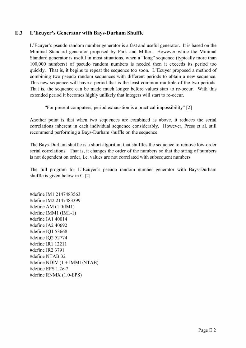
E.3 L’Ecuyer’s Generator with Bays-Durham Shuffle L’Ecuyer’s pseudo random number generator is a fast and useful generator. It is based on the Minimal Standard generator proposed by Park and Miller. However while the Minimal Standard generator is useful in most situations, when a “long” sequence (typically more than 100,000 numbers) of pseudo random numbers is needed then it exceeds its period too quickly. That is, it begins to repeat the sequence too soon. L’Ecuyer proposed a method of combining two pseudo random sequences with different periods to obtain a new sequence. This new sequence will have a period that is the least common multiple of the two periods. That is, the sequence can be made much longer before values start to re-occur. With this extended period it becomes highly unlikely that integers will start to re-occur. “For present computers, period exhaustion is a practical impossibility” [2] Another point is that when two sequences are combined as above, it reduces the serial correlations inherent in each individual sequence considerably. However, Press et al. still recommend performing a Bays-Durham shuffle on the sequence. The Bays-Durham shuffle is a short algorithm that shuffles the sequence to remove low-order serial correlations. That is, it changes the order of the numbers so that the string of numbers is not dependent on order, i.e. values are not correlated with subsequent numbers. The full program for L’Ecuyer’s pseudo random number generator with Bays-Durham shuffle is given below in C [2] #define IM1 2147483563 #define IM2 2147483399 #define AM (1.0/IM1) #define IMM1 (IM1-1) #define IA1 40014 #define IA2 40692 #define IQ1 53668 #define IQ2 52774 #define IR1 12211 #define IR2 3791 #define NTAB 32 #define NDIV (1 + IMM1/NTAB) #define EPS 1.2e-7 #define RNMX (1.0-EPS)

Page E 3

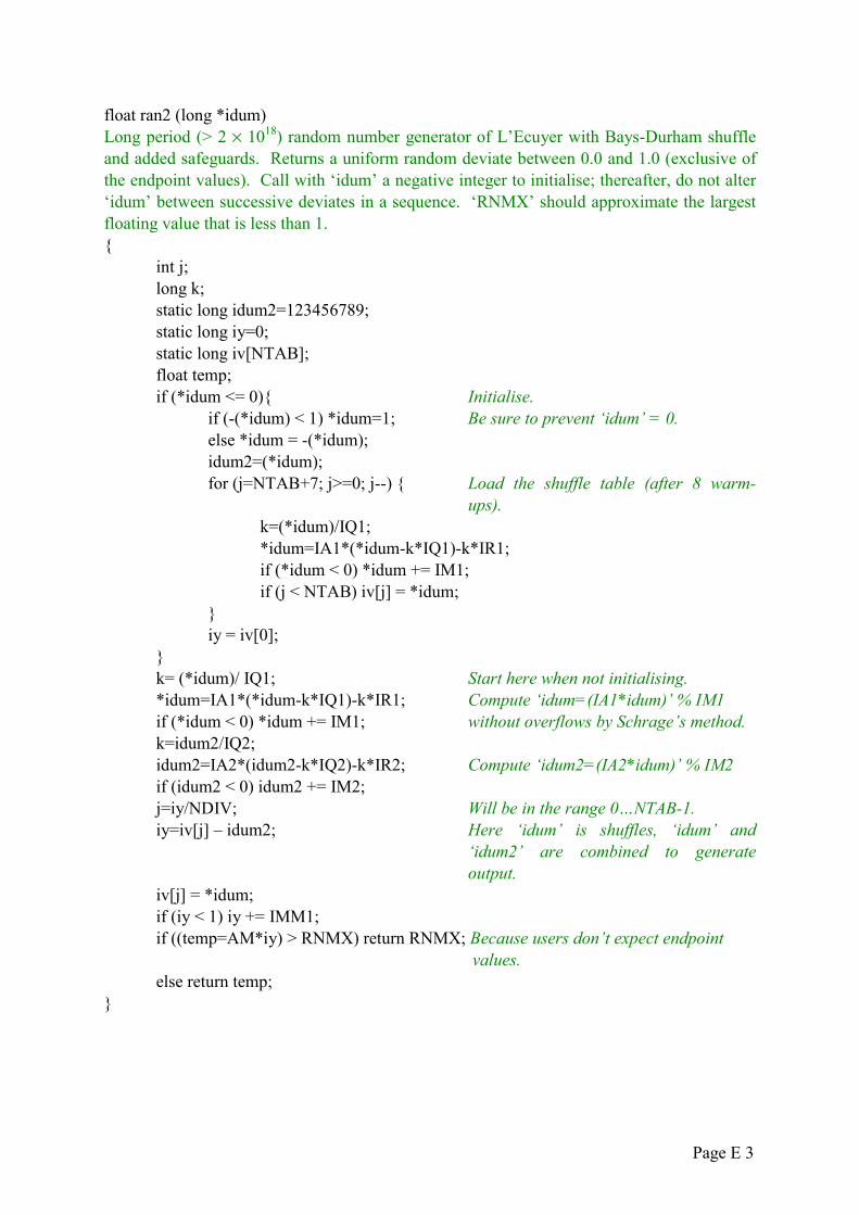
float ran2 (long *idum) Long period (> 2 × 1018) random number generator of L’Ecuyer with Bays-Durham shuffle and added safeguards. Returns a uniform random deviate between 0.0 and 1.0 (exclusive of the endpoint values). Call with ‘idum’ a negative integer to initialise; thereafter, do not alter ‘idum’ between successive deviates in a sequence. ‘RNMX’ should approximate the largest floating value that is less than 1. {

int j; long k; static long idum2=123456789; static long iy=0; static long iv[NTAB]; float temp; if (*idum <= 0){ Initialise.

if (-(*idum) < 1) *idum=1; Be sure to prevent ‘idum’ = 0. else *idum = -(*idum); idum2=(*idum); for (j=NTAB+7; j>=0; j--) { Load the shuffle table (after 8 warm-

ups). k=(*idum)/IQ1; *idum=IA1*(*idum-k*IQ1)-k*IR1; if (*idum < 0) *idum += IM1; if (j < NTAB) iv[j] = *idum;

} iy = iv[0];

} k= (*idum)/ IQ1; Start here when not initialising. *idum=IA1*(*idum-k*IQ1)-k*IR1; Compute ‘idum=(IA1*idum)’ % IM1 if (*idum < 0) *idum += IM1; without overflows by Schrage’s method. k=idum2/IQ2; idum2=IA2*(idum2-k*IQ2)-k*IR2; Compute ‘idum2=(IA2*idum)’ % IM2 if (idum2 < 0) idum2 += IM2; j=iy/NDIV; Will be in the range 0…NTAB-1. iy=iv[j] – idum2; Here ‘idum’ is shuffles, ‘idum’ and

‘idum2’ are combined to generate output.

iv[j] = *idum; if (iy < 1) iy += IMM1; if ((temp=AM*iy) > RNMX) return RNMX; Because users don’t expect endpoint values. else return temp;

}

Page F 1

F. EXPLORATORY DATA ANALYSIS ON LAVARAND.SGI.COM AND L’ECUYER’S PRNG

F.1 Exploratory Data Analysis for 1,000 numbers generated by Lavarand.sgi.com Summary Statistics TABLE F.1.1 Summary Statistics for Lavarand.sgi.com


Duplications Number of Non

Occurring Values 10000 497.832 497 999 0 0.471 267 361 Data Analysis Plots Run Sequence Plot

FIGURE F.1.1 Runs Sequence Plot for Lavarand.sgi.com

Page F 2

Lag Plot

FIGURE F.1.2 Lag Plot for Lavarand.sgi.com Histogram

FIGURE F.1.3 Histogram for Lavarand.sgi.com

Page F 3

Autocorrelation Plot

302010

1.00.80.60.40.20.0

-0.2-0.4-0.6-0.8-1.0

Auto

corre

latio

n

LBQTCorrLagLBQTCorrLagLBQTCorrLagLBQTCorrLag

28.9028.8127.13

27.0226.1825.8025.0423.9421.9316.4115.0714.95

14.4212.21 9.80 9.79 9.19 9.19 9.15 9.14 8.28

7.80 5.98 5.38 4.94 4.94 2.69 2.66 2.01 0.01

0.29 1.24 0.31

-0.88-0.59 0.84 1.01 1.37-2.29-1.13-0.34 0.71

-1.45-1.52-0.12 0.76 0.05 0.20-0.07-0.92 0.68

-1.33 0.76-0.66 0.06 1.49-0.17 0.80-1.41-0.09

0.01 0.04 0.01

-0.03-0.02 0.03 0.03 0.04-0.07-0.04-0.01 0.02

-0.05-0.05-0.00 0.02 0.00 0.01-0.00-0.03 0.02

-0.04 0.02-0.02 0.00 0.05-0.01 0.03-0.04-0.00

302928

272625242322212019

181716151413121110

9 8 7 6 5 4 3 2 1


FIGURE F.1.4 Autocorrelation Plot for Lavarand.sgi.com

F.2 Exploratory Data Analysis for 1,000 numbers generated by L’Ecuyer’s PRNG

Summary Statistics TABLE F.2.1 Summary Statistics for 'Ecuyer's PRNG


Duplications Number of Non

Occurring Values 5000 506.43 511 999 0 0.488 253 349

Page F 4

Data Analysis Plots Run Sequence Plot

FIGURE F.2.1 Runs Sequence Plot for L’Ecuyer’s PRNG Lag Plot

FIGURE F.2.2 Lag Plot for L’Ecuyer’s PRNG

Page F 5

Histogram

FIGURE F.2.3 Histogram for L’Ecuyer’s PRNG Autocorrelation Plot

302010

1.00.80.60.40.20.0

-0.2-0.4-0.6-0.8-1.0

Auto

corre

latio

n

LBQTCorrLagLBQTCorrLagLBQTCorrLagLBQTCorrLag

23.4523.1818.14

18.1215.9812.4811.4611.4410.7810.63 9.89 9.89

9.88 9.18 9.18 9.01 8.86 7.35 7.35 7.03 6.91

5.04 5.04 5.03 5.03 2.23 2.23 1.28 0.96 0.67

-0.50-2.17-0.14

-1.42-1.82 0.99-0.12 0.80-0.38 0.84-0.03 0.09

0.82-0.05 0.41 0.37-1.21-0.05-0.56 0.35-1.35

0.02 0.10-0.00-1.66 0.05 0.97-0.57 0.54-0.82

-0.02-0.07-0.00

-0.05-0.06 0.03-0.00 0.03-0.01 0.03-0.00 0.00

0.03-0.00 0.01 0.01-0.04-0.00-0.02 0.01-0.04

0.00 0.00-0.00-0.05 0.00 0.03-0.02 0.02-0.03

302928

272625242322212019

181716151413121110

9 8 7 6 5 4 3 2 1


FIGURE F.2.4 Autocorrelation Plot for L’Ecuyer’s PRNG

Page G 1

G. DESCRIPTIONS OF THE TESTS USED

G.1 The Chi-Squared Test

The Chi-Squared Distribution, χ2 The sample variance of a data sample x1, x2, x3, …, xN is calculated from the formula:

( )1

1

2

2

−

−=

∑=

n

xxs

n

ii

Where xi is an observation and i = 1 to n

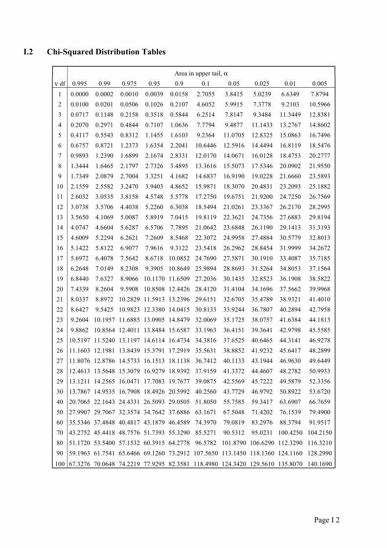
x is the mean of the sample n is the number of observations in the sample. S2 will vary from sample to sample, when the data are normally distributed, and follows a χ2 distribution (the result is squared to emphasis that it cannot be negative.). For other non-normal data then the distribution of s2 can be approximated to the χ2 distribution if the sample size is sufficiently large. Chi-squared depends on a parameter called “degrees of freedom”. The degrees of freedom parameter simply defines a particular chi-squared distribution. The distribution is skewed to the right and has a mean value equal to its degrees of freedom. The percentage point χ2

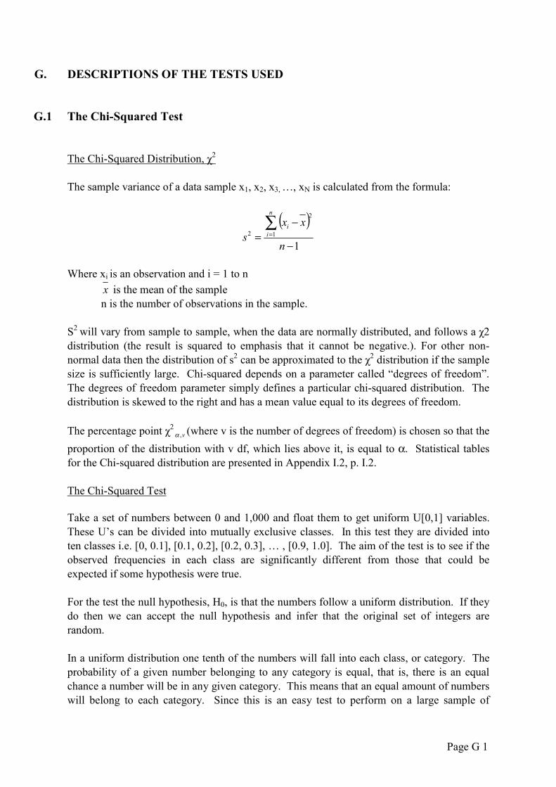
v,α (where v is the number of degrees of freedom) is chosen so that the proportion of the distribution with v df, which lies above it, is equal to α. Statistical tables for the Chi-squared distribution are presented in Appendix I.2, p. I.2. The Chi-Squared Test Take a set of numbers between 0 and 1,000 and float them to get uniform U[0,1] variables. These U’s can be divided into mutually exclusive classes. In this test they are divided into ten classes i.e. [0, 0.1], [0.1, 0.2], [0.2, 0.3], … , [0.9, 1.0]. The aim of the test is to see if the observed frequencies in each class are significantly different from those that could be expected if some hypothesis were true. For the test the null hypothesis, H0, is that the numbers follow a uniform distribution. If they do then we can accept the null hypothesis and infer that the original set of integers are random. In a uniform distribution one tenth of the numbers will fall into each class, or category. The probability of a given number belonging to any category is equal, that is, there is an equal chance a number will be in any given category. This means that an equal amount of numbers will belong to each category. Since this is an easy test to perform on a large sample of

Page G 2

numbers I chose to run the test on 10,000 numbers generated by Random.org. Thus 1,000 numbers are expected in each class. These are the Expected Frequencies, Ei. The next step is to count the numbers of numbers that occur in the sample that belong to each category. These are the Observed Frequencies, Oi. The sum of the expected frequencies will be equal to the sum of the observed frequencies and also equal to the number of numbers in the sample. The chi-squared test statistic is then calculated from the formula:

χ2 ∑=

−=k

i i

ii

EEO

1

2)(

Where k is the number of categories n is the number of observations. The critical value for the test can be found in statistical tables or using Excel. If the test statistic exceeds the critical value then the null hypothesis cannot be accepted. The critical value for this test at the 5% significance level, α = 0.05, with 9 degrees of freedom is:

χ =29,05.0 16.92

The degrees of freedom are calculated by the formula (k-m) where k is the number of categories and m is the number of linear constraints on the test. Here there is one linear constraint due to the fact that the frequency in the last class interval is determined once the frequencies in the first (k-1) classes are known. When the test statistic is less than the critical value the null hypothesis is accepted and the original data sample is deemed to be random.

G.2 The Test of Runs Above and Below the Median This test looks at the order of observations to determine if the order is random or attributable to a pattern in the data. Thus a run is defined as a set of consecutive observations that are either all less than or all greater than some value. This test focuses on runs above and below the median. Observations greater than the median are assigned the letter “a” and observations less that the median are assigned the letter “b”. Observations equal to the median are omitted. Thus the data sample is converted into a series of a’s and b’s in the order of the original data sample. The next step is to calculate u, the total number of runs, n1, the number of a’s and n2, the number of b’s. Then u is distributed with a mean

And a standard deviation

12

21

21 ++

=nnnn

uµ

Page G 3

( )( ) ( )1

22

212

21

212121

−++−−=

nnnnnnnnnn

uσ

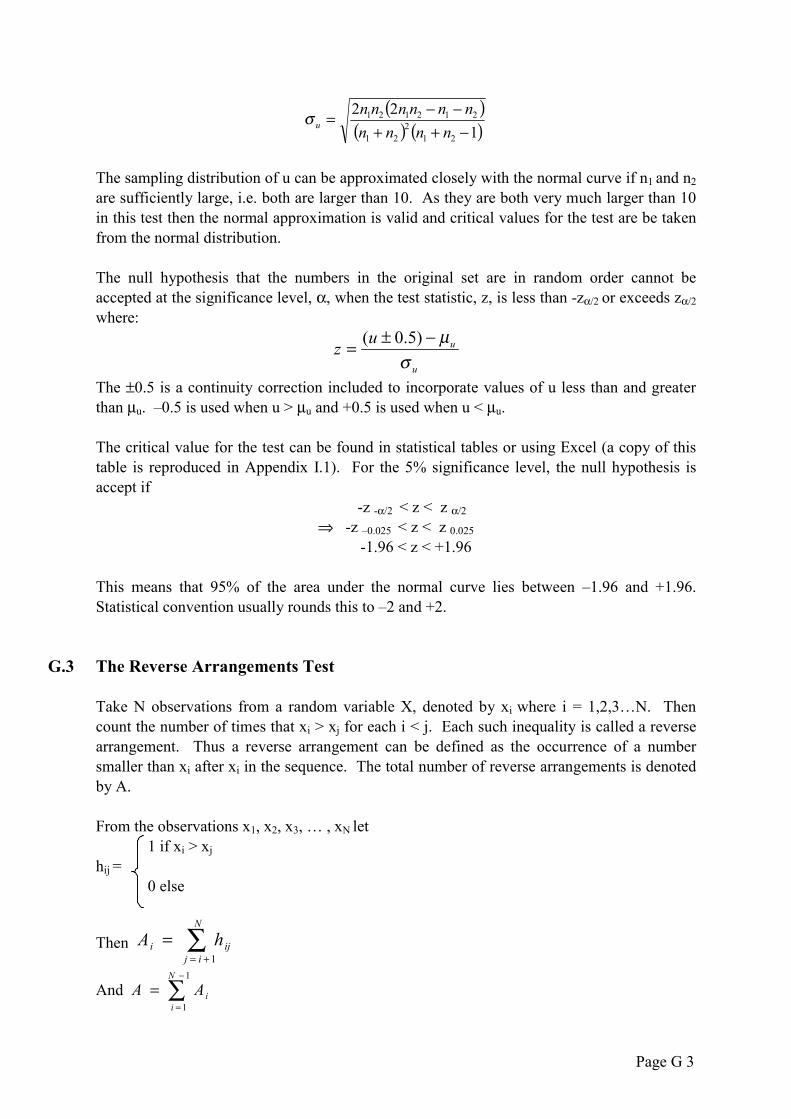
The sampling distribution of u can be approximated closely with the normal curve if n1 and n2

are sufficiently large, i.e. both are larger than 10. As they are both very much larger than 10 in this test then the normal approximation is valid and critical values for the test are be taken from the normal distribution. The null hypothesis that the numbers in the original set are in random order cannot be accepted at the significance level, α, when the test statistic, z, is less than -zα/2 or exceeds zα/2 where:

u

uuzσ

µ−±= )5.0(

The ±0.5 is a continuity correction included to incorporate values of u less than and greater than µu. –0.5 is used when u > µu and +0.5 is used when u < µu. The critical value for the test can be found in statistical tables or using Excel (a copy of this table is reproduced in Appendix I.1). For the 5% significance level, the null hypothesis is accept if

-z -α/2 < z < z α/2 ⇒ -z –0.025 < z < z 0.025

-1.96 < z < +1.96 This means that 95% of the area under the normal curve lies between –1.96 and +1.96. Statistical convention usually rounds this to –2 and +2.

G.3 The Reverse Arrangements Test Take N observations from a random variable X, denoted by xi where i = 1,2,3…N. Then count the number of times that xi > xj for each i < j. Each such inequality is called a reverse arrangement. Thus a reverse arrangement can be defined as the occurrence of a number smaller than xi after xi in the sequence. The total number of reverse arrangements is denoted by A. From the observations x1, x2, x3, … , xN let 1 if xi > xj hij = 0 else

Then ∑+=

=N

ijiji hA

1

And ∑−

=

=1

1

N

iiAA

Page G 4

hij is calculated for each number preceding the current number and summing these h’s gives Ai. Ai is calculated for each observation and the sum of these Ai’s is A, the total number of reverse arrangements. If the sequence of N observations are independent observations on the same random variable, then the number of reverse arrangements, A, is a random variable with a mean

4)1( −= NN

Aµ

And a variance

72

)1)(12(2 −−= NNNAσ

A table for calculating critical values for the reverse arrangements test is given by Bendat and Piersol [3]. Table G.3.1 below gives the section relevant to this test. The full table is given in Appendix I.3, p. I.3. TABLE G.3.1 Percent points of Reverse Arrangement Distribution

N 10 12 14 16 20 30 50 100 AN;0.0975 11 18 27 38 64 162 495 2145 AN;0.025 33 47 63 81 125 272 729 2804

This test is run on the hypothesis that there is no trend in the data sample and that the numbers are thus random. This null hypothesis is accepted if

AN:(1-α/2) < A ≤ AN;( α/2) In this test a sample size, N, of 100 and a significance level, α, of 5% was chosen. Thus in this test the null hypothesis is accepted if

A100;0.975 < A ≤ A100;0.025 From Bendat & Piersol’s table this is

2145 < A ≤ 2804 A sample size of 100 for each experiment was chosen because that was the maximum sample size that the table gave values for.

Page G 5

G.4 The Overlapping Sums Test The N integers are floated to get uniform, U[0,1], variables; U1, U2, U3, … , UN. Then overlapping sums are constructed such that S1 = U1+ U2 + ... + U100 ; S2 = U2+ U3 + ... + U101 etc. These S’s are approximately multivariate normal with a mean vector µ and covariance matrix Σ (this is a result of the Central Limit Theorem). One hundred of these S’s are taken and converted into standard normal variables, Z ~ N(0,1), by pre-multiplying (S - µ) by a matrix A where A is such that ATA = Σ, i.e.

A × (S - µ) ~ N(0,1) These standard normal variates are converted into uniform, U[0,1], variables by the inverse normal cumulative distribution function in order to carry out a chi-squared test. This is repeated five times on five sets of 100 S’s taken from the same generator. One hundred S’s are taken at a time because I was restricted by the size of matrix, A which was only calculated for 100 values. Then all 500 uniforms are given a chi-squared test to test that they follow the uniform distribution closely enough so that it may be concluded that the original data is random. One thing to note is that in every case the mean of the S’s, µ, is 50. This is because Si = Ui+ Ui+1 + ... + Ui+99 ⇒ E[Si] = E[Ui+ Ui+1 + ... + Ui+99] ⇒ E[Si] = E[100*Ui] = 100*E[Ui] Ui is a uniform variable and thus its expected value is 0.5. ⇒ E[Si] = 100*0.5 = 50.

G.5 The Binary Rank Test for 32x32 Matrices

The Rank of a Matrix Two vectors of the same length are said to be “linearly independent” if the elements of one vector are not proportional to those of the second. Thus x = [1, 0, -1] and y = [4, 0, -4] are not linearly independent while u = [2, -1, 0, 7] and v = [6, 2, 0, 0] are. If a matrix is formed from a set of vectors then the degree of linear independence of the set is defined as the rank of the matrix. Thus given any matrix the rank is the number of linear

Page G 6

independent row vectors in the matrix. A matrix’s rank can vary from 0 to K (where K is the total number of row vectors in the matrix). A matrix of rank K is said to be of “full rank”. The Binary Rank Test for 32x32 Matrices The binary rank test uses this concept of ranks to test for randomness in using binary 0’s and 1’s. The first step is to create a 32x32 binary matrix where each row vector of the matrix is a 32-bit integer. Using Matlab the rank of the matrix is easily computed. As mentioned above the rank of the matrix can be between 0 and 32. However, as ranks <29 are rare, their counts are pooled with those for rank 29. A chi-squared test is performed on counts for ranks <29, 30, 31, and 32. The full program used for calculating the rank of the matrices in Matlab is: data = dlmread(Random_numbers.txt',',');

% Replace pseudorandom.txt with the file name of the random numbers % i.e. if your file was numbers.dat then this line should be: % data = dlmread('numbers.dat',','); % The file should be comma delimited

npoints=length(data); % This is the number of values in the file nmatrices = floor(npoints/(32.*32)); % This is the number of matrices that you can build ranks = zeros(nmatrices,1); % Stores the ranks data = data(1:(nmatrices.*32.*32)); % cut off any points at the end of the data that cannot be

used data =reshape(data,32,32.*nmatrices); for (i=1:nmatrices) current_mat = data(:,((i-1).*32+1):(i.*32)); % Extract i-th matrix ranks(i) = rank(current_mat); end nmatrices ranks

Page H1

H. HYPOTHESIS TESTING Evaluating the results of the tests involves a statistical process known as hypothesis testing. When the experiment is carried out there is usually some hypothesis or theory that is being tested. Hypothesis testing follows a structure that makes interpreting statistical test results less complicated. First the null hypothesis and the alternative hypothesis are defined, then the test statistic, the level of significance and the critical value are defined. Usually when an experiment is carried out there are two conflicting theories about the data, one of which the test will aim to disprove. The theory that is being tested is called the null hypothesis, Ho, and the other theory is called the alternative hypothesis, HA. The null hypothesis is so called because it assumes the numbers in the data set are doing what they are supposed to be doing, e.g. following a given distribution, exhibiting a trend, matching the population’s parameters etc. The null hypothesis must be assumed to be true until the results of the tests indicates otherwise. The test statistic is used to put a numerical value on the departure from the null hypothesis. Thus the test statistic allows a judgement to be made about how far the data is from the theory. In order to use the test statistic a level of significance and a critical value must be determined. If the test statistic exceeds the critical value then the null hypothesis is rejected. The conventional level of significance adopted by hypothesis testing is 5%. Thus if a result is significant at the 5% level the null hypothesis is rejected. This level is chosen in most tests because it means that 95% of the values for the test statistic are below the equivalent critical value. Thus the probability of observing a value as or more extreme than the current value is 0.05. If a result is significant at the 5% level then it is generally taken to be reasonable evidence that the null hypothesis is untrue. If the result is significant at the 1% level of significance then it is generally taken to be fairly conclusive evidence that the null hypothesis is untrue.[6]

Page I 1

I. STATISTICAL TABLES

I.1 Normal Distribution Table

z 0.00 0.01 0.02 0.03 0.04 0.05 0.06 0.07 0.08 0.09 0.0 0.0000 0.0040 0.0080 0.0120 0.0160 0.0199 0.0239 0.0279 0.0319 0.0359 0.1 0.0398 0.0438 0.0478 0.0517 0.0557 0.0596 0.0636 0.0675 0.0714 0.0753 0.2 0.0793 0.0832 0.0871 0.0910 0.0948 0.0987 0.1026 0.1064 0.1103 0.1141 0.3 0.1179 0.1217 0.1255 0.1293 0.1331 0.1368 0.1406 0.1443 0.1480 0.1517 0.4 0.1554 0.1591 0.1628 0.1664 0.1700 0.1736 0.1772 0.1808 0.1844 0.1879 0.5 0.1915 0.1950 0.1985 0.2019 0.2054 0.2088 0.2123 0.2157 0.2190 0.2224 0.6 0.2257 0.2291 0.2324 0.2357 0.2389 0.2422 0.2454 0.2486 0.2517 0.2549 0.7 0.2580 0.2611 0.2642 0.2673 0.2704 0.2734 0.2764 0.2794 0.2823 0.2852 0.8 0.2881 0.2910 0.2939 0.2967 0.2995 0.3023 0.3051 0.3078 0.3106 0.3133 0.9 0.3159 0.3186 0.3212 0.3238 0.3264 0.3289 0.3315 0.3340 0.3365 0.3389 1.0 0.3413 0.3438 0.3461 0.3485 0.3508 0.3531 0.3554 0.3577 0.3599 0.3621 1.1 0.3643 0.3665 0.3686 0.3708 0.3729 0.3749 0.3770 0.3790 0.3810 0.3830 1.2 0.3849 0.3869 0.3888 0.3907 0.3925 0.3944 0.3962 0.3980 0.3997 0.4015 1.3 0.4032 0.4049 0.4066 0.4082 0.4099 0.4115 0.4131 0.4147 0.4162 0.4177 1.4 0.4192 0.4207 0.4222 0.4236 0.4251 0.4265 0.4279 0.4292 0.4306 0.4319 1.5 0.4332 0.4345 0.4357 0.4370 0.4382 0.4394 0.4406 0.4418 0.4429 0.4441 1.6 0.4452 0.4463 0.4474 0.4484 0.4495 0.4505 0.4515 0.4525 0.4535 0.4545 1.7 0.4554 0.4564 0.4573 0.4582 0.4591 0.4599 0.4608 0.4616 0.4625 0.4633 1.8 0.4641 0.4649 0.4656 0.4664 0.4671 0.4678 0.4686 0.4693 0.4699 0.4706 1.9 0.4713 0.4719 0.4726 0.4732 0.4738 0.4744 0.4750 0.4756 0.4761 0.4767 2.0 0.4772 0.4778 0.4783 0.4788 0.4793 0.4798 0.4803 0.4808 0.4812 0.4817 2.1 0.4821 0.4826 0.4830 0.4834 0.4838 0.4842 0.4846 0.4850 0.4854 0.4857 2.2 0.4861 0.4864 0.4868 0.4871 0.4875 0.4878 0.4881 0.4884 0.4887 0.4890 2.3 0.4893 0.4896 0.4898 0.4901 0.4904 0.4906 0.4909 0.4911 0.4913 0.4916 2.4 0.4918 0.4920 0.4922 0.4925 0.4927 0.4929 0.4931 0.4932 0.4934 0.4936 2.5 0.4938 0.4940 0.4941 0.4943 0.4945 0.4946 0.4948 0.4949 0.4951 0.4952 2.6 0.4953 0.4955 0.4956 0.4957 0.4959 0.4960 0.4961 0.4962 0.4963 0.4964 2.7 0.4965 0.4966 0.4967 0.4968 0.4969 0.4970 0.4971 0.4972 0.4973 0.4974 2.8 0.4974 0.4975 0.4976 0.4977 0.4977 0.4978 0.4979 0.4979 0.4980 0.4981 2.9 0.4981 0.4982 0.4982 0.4983 0.4984 0.4984 0.4985 0.4985 0.4986 0.4986

3.0 0.4987 0.4987 0.4987 0.4988 0.4988 0.4989 0.4989 0.4989 0.4990 0.4990

Page I 2

I.2 Chi-Squared Distribution Tables

Area in upper tail, α ν df 0.995 0.99 0.975 0.95 0.9 0.1 0.05 0.025 0.01 0.005

1 0.0000 0.0002 0.0010 0.0039 0.0158 2.7055 3.8415 5.0239 6.6349 7.8794 2 0.0100 0.0201 0.0506 0.1026 0.2107 4.6052 5.9915 7.3778 9.2103 10.5966 3 0.0717 0.1148 0.2158 0.3518 0.5844 6.2514 7.8147 9.3484 11.3449 12.8381 4 0.2070 0.2971 0.4844 0.7107 1.0636 7.7794 9.4877 11.1433 13.2767 14.8602 5 0.4117 0.5543 0.8312 1.1455 1.6103 9.2364 11.0705 12.8325 15.0863 16.7496 6 0.6757 0.8721 1.2373 1.6354 2.2041 10.6446 12.5916 14.4494 16.8119 18.5476 7 0.9893 1.2390 1.6899 2.1674 2.8331 12.0170 14.0671 16.0128 18.4753 20.2777 8 1.3444 1.6465 2.1797 2.7326 3.4895 13.3616 15.5073 17.5346 20.0902 21.9550 9 1.7349 2.0879 2.7004 3.3251 4.1682 14.6837 16.9190 19.0228 21.6660 23.5893

10 2.1559 2.5582 3.2470 3.9403 4.8652 15.9871 18.3070 20.4831 23.2093 25.1882 11 2.6032 3.0535 3.8158 4.5748 5.5778 17.2750 19.6751 21.9200 24.7250 26.7569 12 3.0738 3.5706 4.4038 5.2260 6.3038 18.5494 21.0261 23.3367 26.2170 28.2995 13 3.5650 4.1069 5.0087 5.8919 7.0415 19.8119 22.3621 24.7356 27.6883 29.8194 14 4.0747 4.6604 5.6287 6.5706 7.7895 21.0642 23.6848 26.1190 29.1413 31.3193 15 4.6009 5.2294 6.2621 7.2609 8.5468 22.3072 24.9958 27.4884 30.5779 32.8013 16 5.1422 5.8122 6.9077 7.9616 9.3122 23.5418 26.2962 28.8454 31.9999 34.2672 17 5.6972 6.4078 7.5642 8.6718 10.0852 24.7690 27.5871 30.1910 33.4087 35.7185 18 6.2648 7.0149 8.2308 9.3905 10.8649 25.9894 28.8693 31.5264 34.8053 37.1564 19 6.8440 7.6327 8.9066 10.1170 11.6509 27.2036 30.1435 32.8523 36.1908 38.5822 20 7.4339 8.2604 9.5908 10.8508 12.4426 28.4120 31.4104 34.1696 37.5662 39.9968 21 8.0337 8.8972 10.2829 11.5913 13.2396 29.6151 32.6705 35.4789 38.9321 41.4010 22 8.6427 9.5425 10.9823 12.3380 14.0415 30.8133 33.9244 36.7807 40.2894 42.7958 23 9.2604 10.1957 11.6885 13.0905 14.8479 32.0069 35.1725 38.0757 41.6384 44.1813 24 9.8862 10.8564 12.4011 13.8484 15.6587 33.1963 36.4151 39.3641 42.9798 45.5585 25 10.5197 11.5240 13.1197 14.6114 16.4734 34.3816 37.6525 40.6465 44.3141 46.9278 26 11.1603 12.1981 13.8439 15.3791 17.2919 35.5631 38.8852 41.9232 45.6417 48.2899 27 11.8076 12.8786 14.5733 16.1513 18.1138 36.7412 40.1133 43.1944 46.9630 49.6449 28 12.4613 13.5648 15.3079 16.9279 18.9392 37.9159 41.3372 44.4607 48.2782 50.9933 29 13.1211 14.2565 16.0471 17.7083 19.7677 39.0875 42.5569 45.7222 49.5879 52.3356 30 13.7867 14.9535 16.7908 18.4926 20.5992 40.2560 43.7729 46.9792 50.8922 53.6720 40 20.7065 22.1643 24.4331 26.5093 29.0505 51.8050 55.7585 59.3417 63.6907 66.7659 50 27.9907 29.7067 32.3574 34.7642 37.6886 63.1671 67.5048 71.4202 76.1539 79.4900 60 35.5346 37.4848 40.4817 43.1879 46.4589 74.3970 79.0819 83.2976 88.3794 91.9517 70 43.2752 45.4418 48.7576 51.7393 55.3290 85.5271 90.5312 95.0231 100.4250 104.2150 80 51.1720 53.5400 57.1532 60.3915 64.2778 96.5782 101.8790 106.6290 112.3290 116.3210 90 59.1963 61.7541 65.6466 69.1260 73.2912 107.5650 113.1450 118.1360 124.1160 128.2990

100 67.3276 70.0648 74.2219 77.9295 82.3581 118.4980 124.3420 129.5610 135.8070 140.1690

Page I 3

Entries in the table give χ2α values, in which α is the area or probability in the upper tail of the chi-square distribution. For example, with 10 degrees of freedom and an area of 0.01 in the upper tail, χ20.01 = 23.2093.

I.3 Reverse Arrangements Distribution Tables

Critical Values for the Reverse Arrangement Distribution

α N

0.99 0.975 0.95 0.05 0.025 0.01 10 9 11 13 31 33 35 12 16 18 21 44 47 49 14 24 27 30 60 63 66 16 34 38 40 78 81 85 18 45 50 54 98 102 107 20 59 64 69 120 125 130 30 152 162 171 263 272 282 40 290 305 319 460 474 489 50 473 495 514 710 729 751 60 702 761 756 1013 1038 1067 70 977 1014 1045 1369 1400 1437 80 1299 1344 1382 1777 1815 1860 90 1668 1721 1766 2238 2283 2336 100 2083 2145 2198 2751 2804 2866

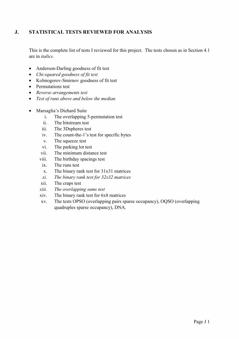
Page J 1

J. STATISTICAL TESTS REVIEWED FOR ANALYSIS This is the complete list of tests I reviewed for this project. The tests chosen as in Section 4.1 are in italics. • Anderson-Darling goodness of fit test • Chi-squared goodness of fit test • Kolmogorov-Smirnov goodness of fit test • Permutations test • Reverse arrangements test • Test of runs above and below the median • Marsaglia’s Diehard Suite

i. The overlapping 5-permutation test ii. The bitstream test

iii. The 3Dspheres test iv. The count-the-1’s test for specific bytes v. The squeeze test

vi. The parking lot test vii. The minimum distance test

viii. The birthday spacings test ix. The runs test x. The binary rank test for 31x31 matrices xi. The binary rank test for 32x32 matrices

xii. The craps test xiii. The overlapping sums test xiv. The binary rank test for 6x8 matrices xv. The tests OPSO (overlapping pairs sparse occupancy), OQSO (overlapping

quadruples sparse occupancy), DNA.

Page K 1

K. GLOSSARY Autocorrelation Correlation is the relationship between two variables. Autocorrelation is the correlation of a variable with itself over successive time intervals. Bit In Computer Science this refers to a single character of a language having just two characters, as either of the binary digits 0 or 1. Byte A sequence of 8 bits (enough to represent one character of alphanumeric data) processed as a single unit of information. Chi-square A test statistic that is calculated as the sum of the squares of observed values minus expected values divided by the expected values. Cryptography The practise and study of encryption and decryption - encoding data so that it can only be decoded by specific individuals. Degrees of freedom A parameter that defines a particular chi-squared distribution. Distributed systems A collection of machines whose distribution is transparent to the user so that the system appears as one local machine. This is in contrast to a network, where the user is aware that there are several machines, and their location, storage replication, load balancing and functionality is not transparent. Distributed systems usually use some kind of client-server organisation. Entropy The measure of a system's energy that is unavailable for work. Since work is obtained from order, the amount of entropy is also a measure of the disorder, or randomness, of a system. Entropy is an extensive property; that is, its magnitude varies from zero to the total amount of energy within a system.

Page K 2

Histogram A bar chart that represents a frequency distribution. The heights of the bars represent observed frequencies Lag plot A lag is a fixed time displacement and the most commonly used lag is 1. A lag plot is a plot of the values of Y(i) versus Y(i-1):

• Vertical axis: Y(i) for all i • Horizontal axis: Y(i-1) for all i

Mean The average value of a set of numbers. Monotonic Trend A trend that is consistently increasing or decreasing in value. Non-parametric Involving no estimation of the parameters of a statistic. Note: Statistical methods that require no (or virtually no) assumptions about the population sampled are usually less efficient than standard techniques that make several assumptions. Non-parametric methods tend to be wasteful of information. It is generally true that the less that is assumed, the less that can be inferred from the data, but it must also be recognised that the more that is assumed, the more the applicability of the method becomes limited. Outlier An extreme deviation from the mean or a very unexpected observation. Parallel processing The simultaneous use of more than one computer to solve a problem. Run sequence plot The run sequence plot is a graph of each observation against the order it is in the sequence. Run sequence plots are formed by:

• Vertical axis: Response variable Y(i) • Horizontal axis: Index i (i = 1, 2, 3, ... )

Page K 3

Sample size The number of units in a population to be studied. The sample size should be big enough to have a high likelihood of detecting a true difference between two groups. Standard deviation A statistic used as a measure of the dispersion or variation in a distribution Summary statistics Summary statistics are a numeric reduction of a data set. Quite commonly, its purpose is to simply arrive at a few key statistics (for example, mean and standard deviation) that may then either replace the data set on archives or carry the summary statistic along in a summary table. Theoretical tests Tests concerned primarily with theories or hypotheses rather than practical considerations; Empirical tests Tests derived from, or relating to, experiment and observation rather than theory. Hypothesis testing A supposition that appears to explain a group of phenomena and is advanced as a basis for further investigation, a proposition that is subject to proof or to an experimental or statistical test. A hypothesis is generally not yet verified, but if it were true, would explain certain facts or phenomena.

REFERENCES [1] Knuth, D.E., The Art of Computer Programming, vol. 2 Seminumerical Methods,

Addison-Wesley, 3rd ed., chpt. 3, 1998. [2] Press W.H., Teukolsky S.A., Vetterling W.T., Flannery B.P., Numerical Recipes in C:

The Art of Scientific Computing, Cambridge University Press, 2nd ed., pp 274,282, 1992.

[3] Bendat J.S. and Piersol A.G., Random Data: Analysis and Measurement Procedures,

Wiley-Interscience, 3rd ed., pp. 99-108, 564, 2000. [4] Lindgern, B.W., Statistical Theory, Chapman and Hall, 4th ed., pp 452-459, 1993. [5] Freund, J.E., Modern Elementary Statistics, Prentice-Hall, 5th ed., pp. 344-348, 1979. [6] Chatfield, C., Statistics for Technology, Chapman and Hall, 3rd ed., pp116-117, 134-

140, 148-155, 332-337 and 1983. [7] The Engineering Statistics Handbook, www.itl.nist.gov/div898/handbook. [8] George Marsaglia’s Diehard Page, http://stat.fsu.edu/~geo/. [9] The Distributed Systems Group Homepage, http://www.dsg.cs.tcd.ie/. [10] Random.org generator website, http://www.random.org. [11] Silicon Graphics Incorporated Random Number Generator, http://lavarand.sgi.com.

http://www.itl.nist.gov/div898/handbook

http://stat.fsu.edu/~geo/

http://www.dsg.cs.tcd.ie/


http://lavarand.sgi.com/

Documents

THE DISTRIBUTED SYSTEMS GROUP, Computer … COLLEGE DUBLIN Management Science and Information Systems Studies Project Report THE DISTRIBUTED SYSTEMS GROUP, Computer Science Department,