The Discretization Process

• Introduction

• Geometric Discretization

• Equation Discretization

• The Finite Difference Method

• The Finite Volume Method

• Solving the Equation

• Conclusion

Task

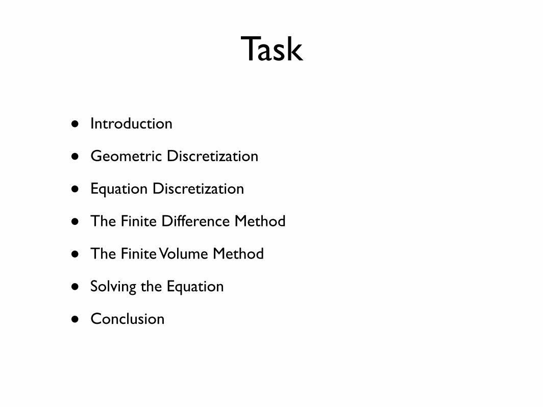
Structured Grids

Cartesian Structured Grid

Non-Orthogonal Structured Grid

Non-Uniform Cartesian Structured Grid

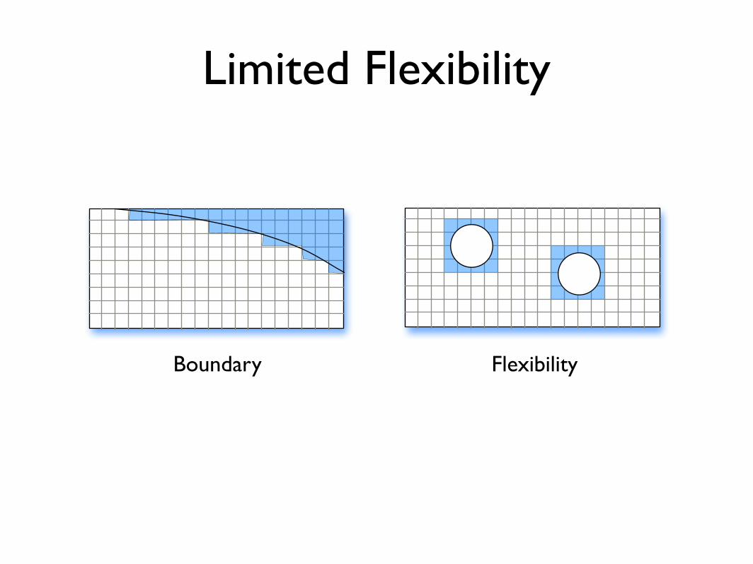
Limited Flexibility

Boundary Flexibility

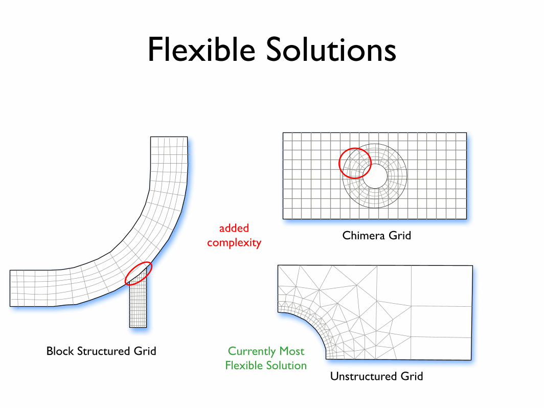
Flexible Solutions

Block Structured Grid

Chimera Grid

Unstructured Grid

added complexity

Currently Most Flexible Solution

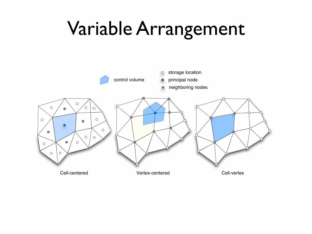
Variable Arrangement

Cell-centered Vertex-centered Cell-vertex

control volume

storage location

principal node

neighboring nodes

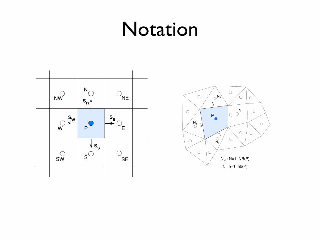
Notation

P

N1

f4

N3

N2

f2

f3

f1

N4

NN : N=1..NB(P)

fn : n=1..nb(P)

P EW

N

SSE

NE

SW

NW

Se

Sn

Sw

Ss

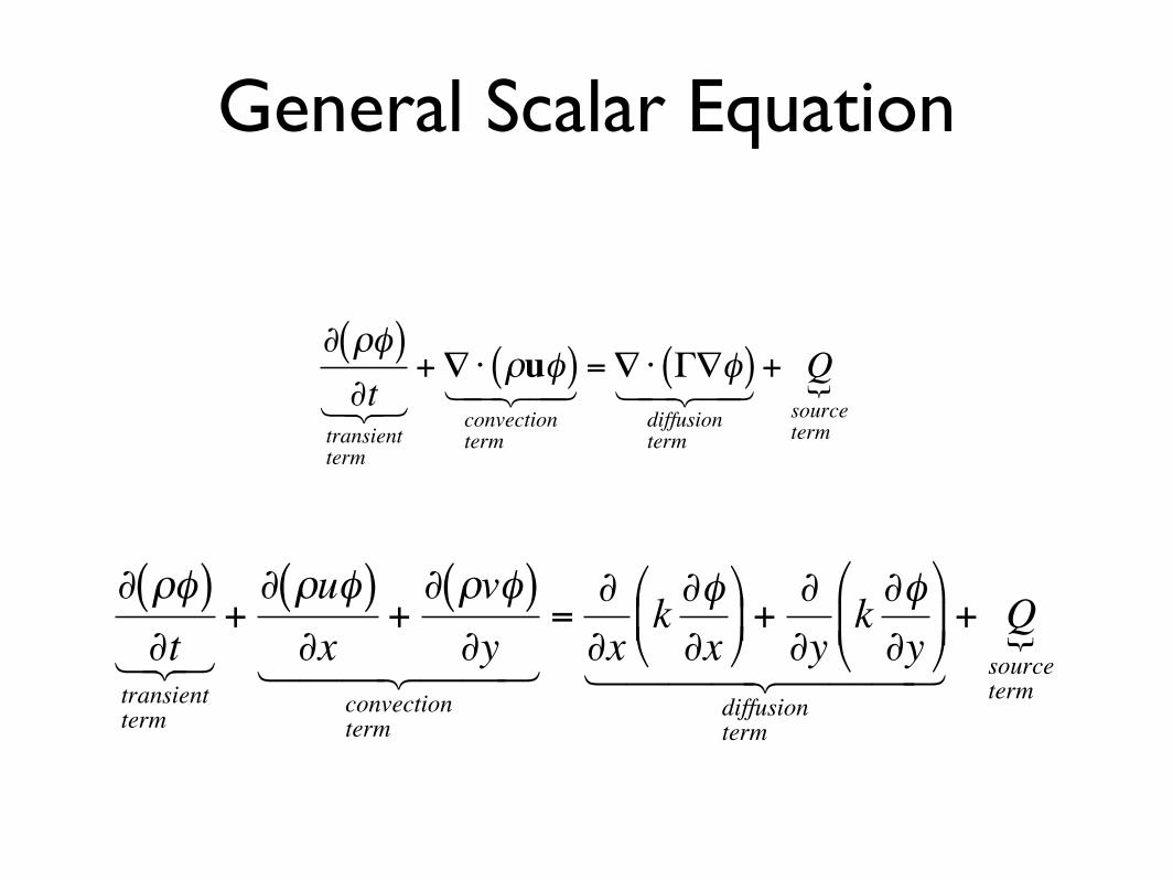
General Scalar Equation

€

∂ ρφ( )∂t

transientterm

1 2 3 +∇ ⋅ ρuφ( )

convectionterm

1 2 4 3 4 =∇ ⋅ Γ∇φ( )

diffusionterm

1 2 4 3 4 + Q

sourceterm

{

€

∂ ρφ( )∂t

transientterm

1 2 3 +∂ ρuφ( )∂x

+∂ ρvφ( )∂y

convectionterm

1 2 4 4 3 4 4 =∂∂x

k ∂φ∂x

+

∂∂y

k ∂φ∂y

diffusionterm

1 2 4 4 4 3 4 4 4

+ Qsourceterm

{

€

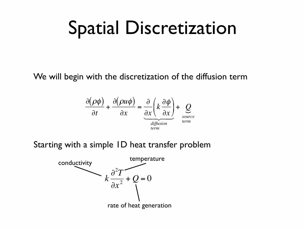
∂ ρφ( )∂t

+∂ ρuφ( )∂x

=∂∂x

k ∂φ∂x

diffusionterm

1 2 4 3 4 + Q

sourceterm

{

Spatial Discretization

€

k ∂2T∂x 2

+Q = 0

We will begin with the discretization of the diffusion term

Starting with a simple 1D heat transfer problem

temperature

rate of heat generation

conductivity

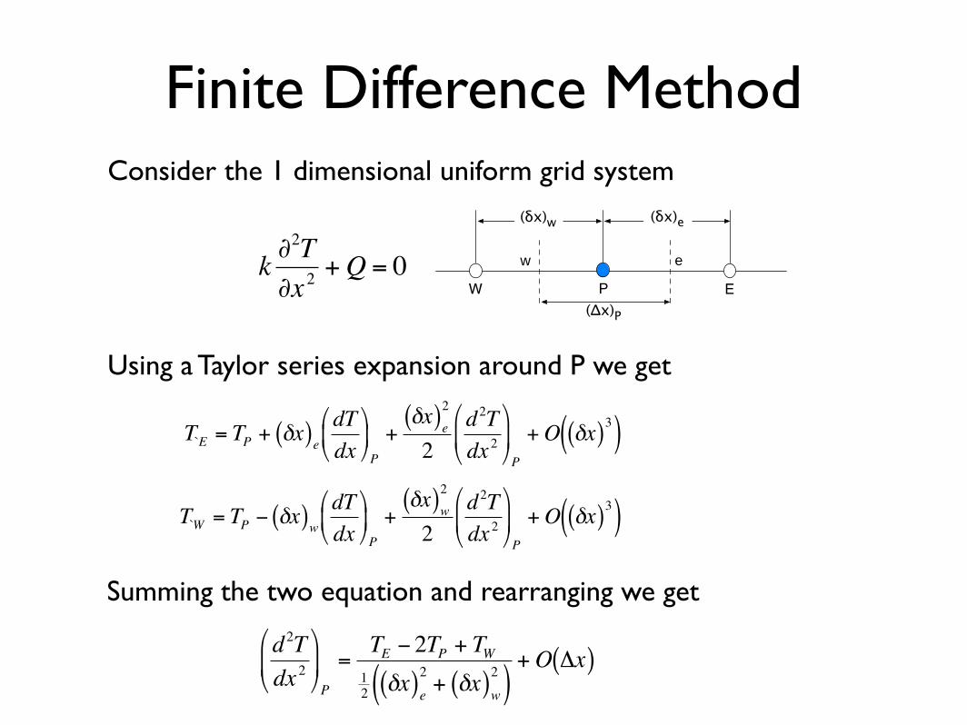
Finite Difference Method

€

T`E = TP + δx( )edTdx

P

+δx( )e

2

2d2Tdx 2

P

+O δx( )3( )

€

TW = TP − δx( )wdTdx

P

+δx( )w

2

2d2Tdx 2

P

+O δx( )3( )

Consider the 1 dimensional uniform grid system

Using a Taylor series expansion around P we get

€

d2Tdx 2

P

=TE − 2TP + TW12 δx( )e

2+ δx( )w

2( )+O Δx( )

Summing the two equation and rearranging we get

P

ew

W E

(!x)w (!x)e

("x)P

€

k ∂2T∂x 2

+Q = 0

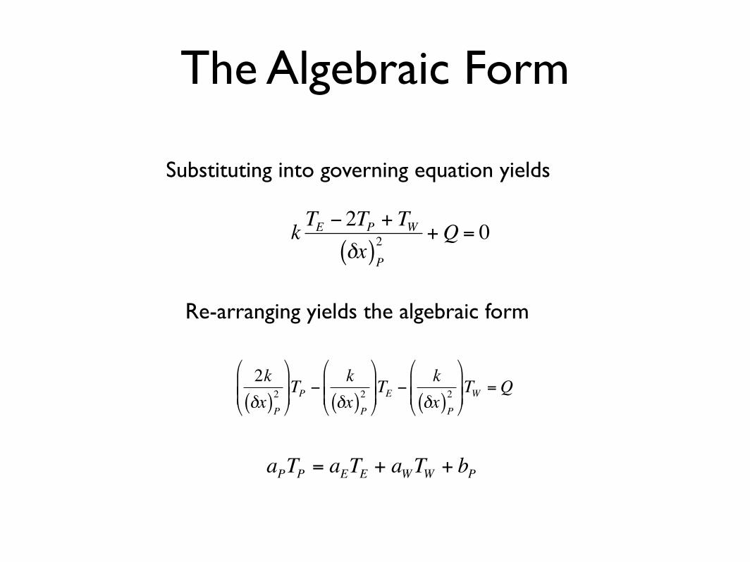
The Algebraic Form

€

k TE − 2TP + TWδx( )P

2 +Q = 0

Substituting into governing equation yields

€

2kδx( )P

2

TP −

kδx( )P

2

TE −

kδx( )P

2

TW =Q

Re-arranging yields the algebraic form

€

aPTP = aETE + aWTW + bP

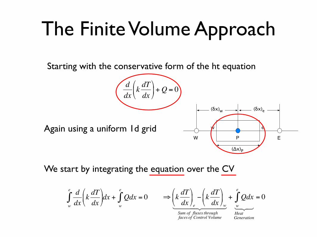
The Finite Volume Approach

€

ddx

k dTdx

+Q = 0

Starting with the conservative form of the ht equation

Again using a uniform 1d gridP

ew

W E

(!x)w (!x)e

("x)P

We start by integrating the equation over the CV

€

ddx

k dTdx

w

e

∫ dx + Qdxw

e

∫ = 0

€

⇒ k dTdx

e

− k dTdx

w

Sum of fluxes throughfaces of Control Volume

1 2 4 4 4 3 4 4 4

+ Qdxw

e

∫HeatGeneration

1 2 3

= 0

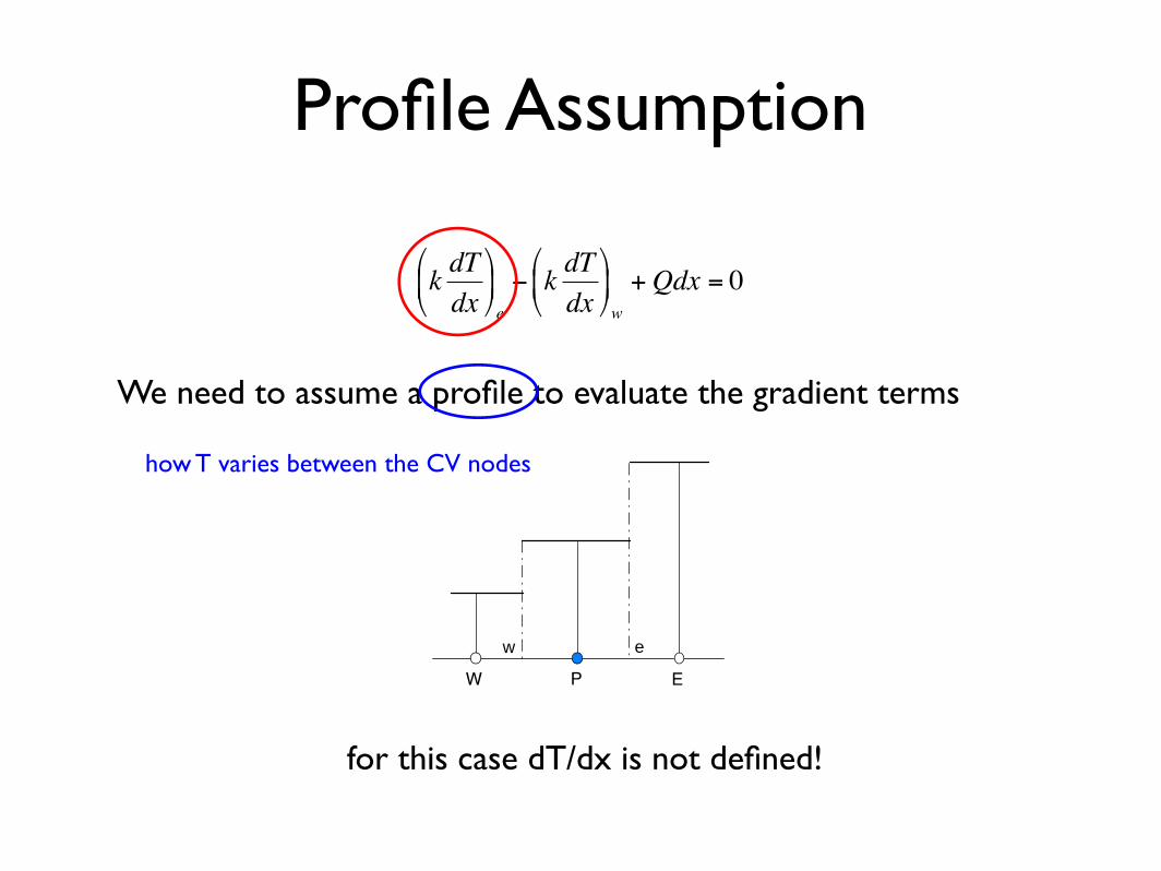
Profile Assumption

€

k dTdx

e

− k dTdx

w

+Qdx = 0

We need to assume a profile to evaluate the gradient terms

P

ew

W E

for this case dT/dx is not defined!

how T varies between the CV nodes

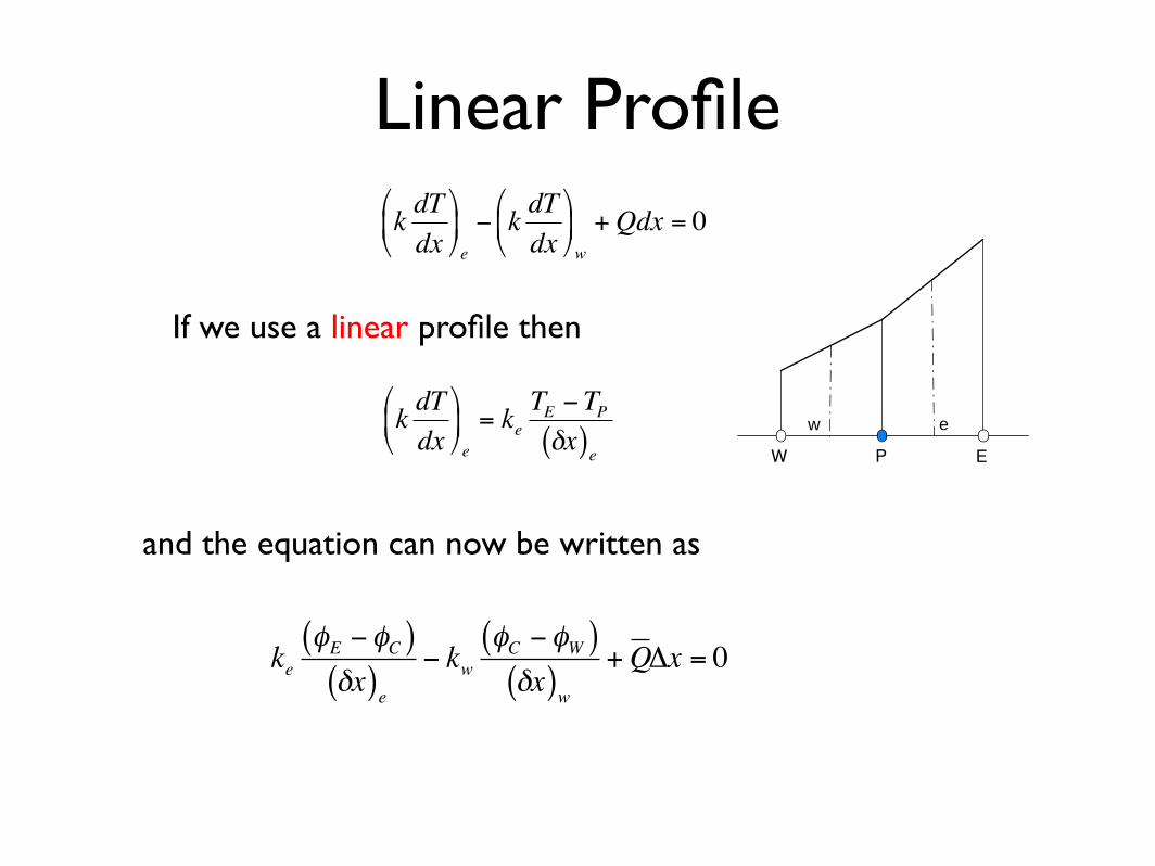
Linear Profile

P

ew

W E

If we use a linear profile then

€

k dTdx

e

= keTE −TPδx( )e

€

k dTdx

e

− k dTdx

w

+Qdx = 0

and the equation can now be written as

€

keφE −φC( )δx( )e

− kwφC −φW( )δx( )w

+QΔx = 0

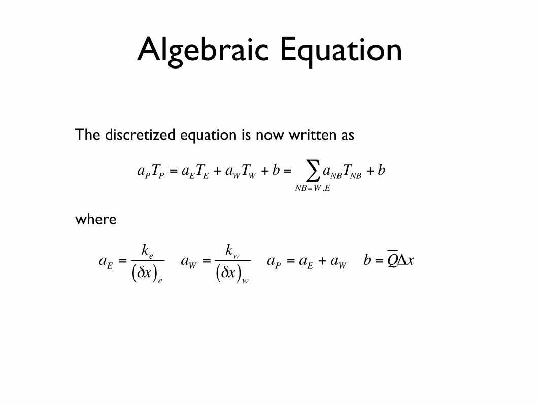
Algebraic Equation

€

aPTP = aETE + aWTW + b = aNBTNBNB=W ,E∑ + b

The discretized equation is now written as

where

€

aE =keδx( )e

aW =kwδx( )w

aP = aE + aW b =QΔx

Convection and Diffusion

€

ddx

ρuφ( ) =ddx

k dφdx

let us extend the discretization to the convection term

P

ew

W E

(!x)w (!x)e

("x)P

€

ρuφ( )e − ρuφ( )w = k dφdx

e

− k dφdx

w

Integrating the equation over the CV yields

Linear Profile

P

ew

W E

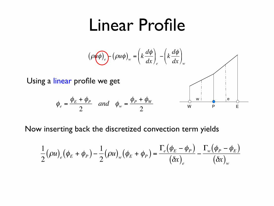
Using a linear profile we get

€

φe =φE + φP2

and φw =φP + φW2

€

ρuφ( )e − ρuφ( )w = k dφdx

e

− k dφdx

w

Now inserting back the discretized convection term yields

€

12ρu( )e φE + φP( ) − 12

ρu( )w φE + φP( ) =Γe φE −φP( )

δx( )e−Γw φP −φE( )

δx( )w

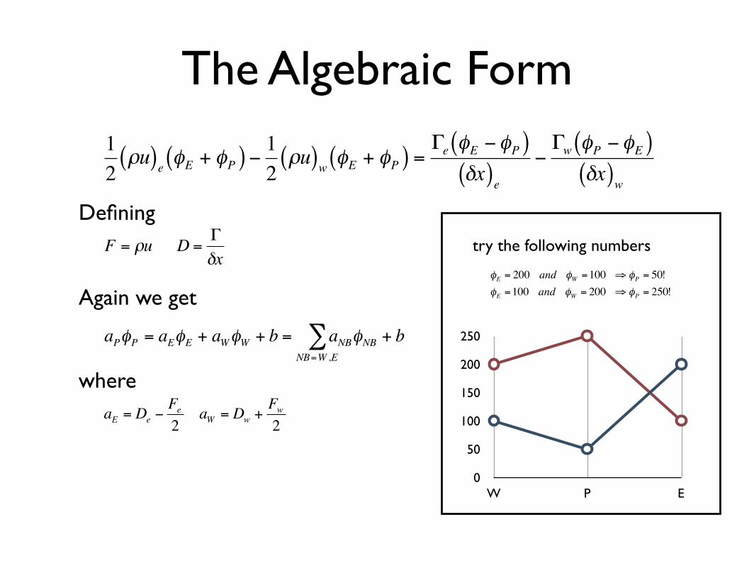
The Algebraic Form

€

12ρu( )e φE + φP( ) − 12

ρu( )w φE + φP( ) =Γe φE −φP( )

δx( )e−Γw φP −φE( )

δx( )w

€

F = ρu D =Γδx

Defining

€

aPφP = aEφE + aWφW + b = aNBφNBNB=W ,E∑ + b

Again we get

€

aE = De −Fe2

aW = Dw +Fw2

where

€

φE = 200 and φW =100 ⇒φP = 50!φE =100 and φW = 200 ⇒φP = 250!

try the following numbers

W P E0

50

100

150

200

250

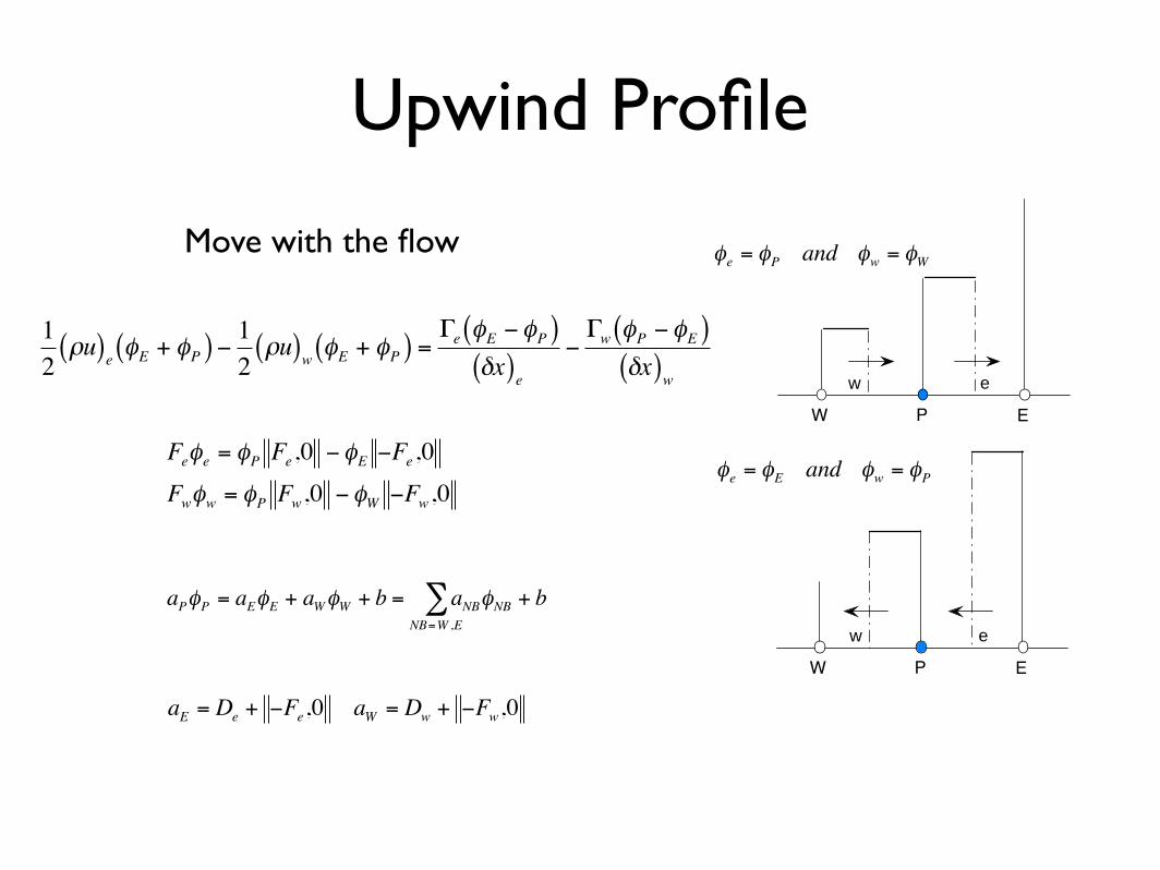
Upwind Profile

P

ew

W E

P

ew

W E

€

φe = φE and φw = φP

€

φe = φP and φw = φW

€

Feφe = φP Fe,0 −φE −Fe,0Fwφw = φP Fw,0 −φW −Fw,0

€

aPφP = aEφE + aWφW + b = aNBφNBNB=W ,E∑ + b

€

aE = De + −Fe,0 aW = Dw + −Fw,0

Move with the flow

€

12ρu( )e φE + φP( ) − 12

ρu( )w φE + φP( ) =Γe φE −φP( )

δx( )e−Γw φP −φE( )

δx( )w

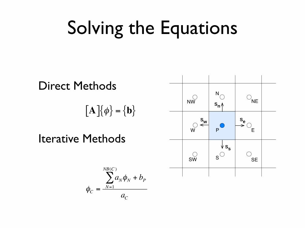
Solving the Equations

Direct Methods

Iterative Methods€

A[ ] φ{ } = b{ }

€

φC =

aNφNN=1

NB(C )

∑ + bP

aC

P EW

N

SSE

NE

SW

NW

Se

Sn

Sw

Ss

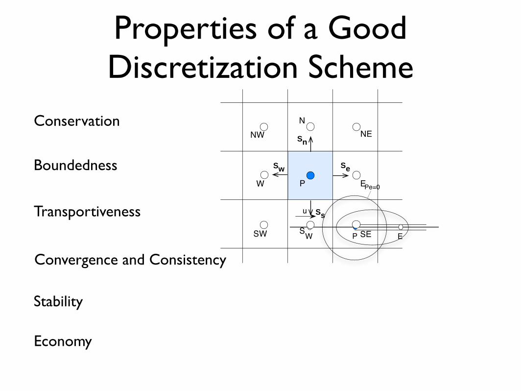
Properties of a Good Discretization Scheme

Conservation

Boundedness

Transportiveness

PW E

u

Pe=0

Convergence and Consistency

Stability

Economy

P EW

N

SSE

NE

SW

NW

Se

Sn

Sw

Ss