Embed Size (px)
Citation preview

THE DEVELOPMENT OF FT-RAMAN TECHNIQUES TO QUANTIFY THE
HYDROLYSIS OF COBALT(III) NITROPHENYLPHOSPHATE
COMPLEXES USING MULTIVARIATE DATA ANALYSIS
by
OUPA SAMUEL TSHABALALA
Submitted in fulfilment of the requirements for
the degree
MASTER OF SCIENCE
in the subject
CHEMISTRY
at the
UNIVERSITY OF SOUTH AFRICA
SUPERVISOR: PROFESSOR S. 0. PAUL (PhD)
JOINT SUPERVISOR: PROFESSOR F. TAFESSE (PhD)
MARCH 2007

DECLARATION
Student number: 35315377
I declare that THE DEVELOPMENT OF FT-RAMAN TECHNIQUES TO
QUANTIFY THE HYDROLYSIS OF COBALT(III) NITROPHENYL
PHOSPHATE COMPLEXES USING MULTIVARIATE DATA ANALYSIS is
my own work and that all the sources that I have used or quoted
have been indicated and acknowledged by means of complete
references.
··~·················· 1v!Jl>/0r ...... l .. ~ ..... ······················ SIGNATURE DATE
(Mr O.S. Tshabalala)
11

ACKNOWLEDGEMENTS
It is not possible for me to mention all people who contributed or
added value to my academic, social and spiritual life towards the
completion of this dissertation. As a matter of fact this work would
not be fruitful, educational and memorable without wisdom and
intelligence of some coaching and positive criticism. In nutshell, I
would like to express my sincere and fraternal gratitude to the
following people:
Above all: I thank my Father God, and my Lord Jesus Christ, and
my comforter the Holy Spirit for revealing the purpose of my
existence and life. JESUS IS LORD!
Professor S. 0. Paul (PhD), my Supervisor: for her expertise in
Vibrational Spectroscopy and its related theory, and Chemometrics;
for her availability and guidance in my research work.
Professor F. Tafesse (PhD), my Joint-Supervisor: for his expertise in
the field of Inorganic Chemistry, and metal-organophosphates
complexes; for his advices and guidance in my research work.
Mr D. C. Lilies (Dave), crystallography specialist form the
Department of Chemistry (University of Pretoria, RSA), for his
availability to determine the structure of [Co(tn)2C03 ]CI04 using
crystallographic method.
The University of South Africa (UNISA), in particular, the
Department of Chemistry for their financial contribution in my MSc
studies. Moreover, Chemistry department staff, Colleagues and
Friends for all their direct and/or indirect support.
iii

The Tshabalala family: I give gratitude to my wife Mokgadi and
my daughter Bontle, my parents Wilson and Magdalene, my brother
Abram and my sister Linda, for their encouragement and support in
my studies.
IV

ABSTRACT
The FT-Raman techniques were developed to quantify reactions that
follow on mixing aqueous solutions of bis-(1,3-diaminopropane)
diaquacobalt(III) ion ([Co(tn)2(0H)(H20)]2+) and p-nitrophenyl
phosphate (PNPP).
For the development and validation of the kinetic modelling
technique, the well-studied inversion of sucrose was utilized. Rate
constants and concentrations could be estimated using calibration
solutions and modelling methods. It was found that the results
obtained are comparable to literature values. Hence this technique
could be further used for the [Co(tn)2(0H)(H20)]2+ assisted
hydrolysis of PNPP.
It was found that rate constants where the pH is maintained at 7.30
give results which differ from those where the pH is started at 7.30
and allowed to change during the reaction. The average rate
constant for 2:1 ([Co(tn)2(0H)(H20)]2+:PNPP reactions was found to
be approximately 3 x 10⁴ times the unassisted PNPP hydrolysis rate.
Keywords: FT-Raman, kinetic modelling, partial least squares,
multivariate data analysis, sucrose hydrolysis, p
nitrophenylphosphate, p-nitrophenol, cobalt(III)
complex, organophosphate ester hydrolysis, pseudo
first order rate constant and second order rate constant.
v

TABLE OF CONTENTS
DECLARATION ................................................................................................ ii
ACKNOWLEDGEMENTS ................................................................................ iii
ABSTRACT AND KEYWORDS ....................................................................... v
TABLE OF CONTENTS ................................................................................... vi
LIST OF TABLES ............................................................................................. ix
LIST OF FIGURES .......................................................................................... xi
LIST OF ACRONYMS ..................................................................................... xv
CHAPTER 1 Introduction ............................................................................... l
1.1 Research motivation ................................................................ l
1.2 Statement of problem ............................................................. 2
1.3 Literature review on applications of Raman spectroscopy
and Multivariate Data Analysis (MDA) in organo-
phosphates ................................................................................. 3
1.4 Research objectives ................................................................ .4
CHAPTER 2 Historical and theoretical aspects of FT-Raman
spectroscopy and multivariate data analysis ..................... 5
2.1 FT-Raman techniques and multivariate data analysis .... 5
2.2 FT-Raman spectroscopy .......................................................... 6
2.2.1 History of Raman spectroscopy development. .................. 6
2.2.2 Basic concepts ........................................................................... 6
2.2.3 Advantages of FT-Raman spectroscopy ............................ 10
2.3 Partial least squares version of multivariate data
analysis ..................................................................................... 11
2.3.1 Historical background ............................................................ 11
2.3.2 Basic principles ....................................................................... 12
2.3.3 PLS regression model. ........................................................... 14
2.3.4 Number of components, correlation of variables and
prediction error ...................................................................... 15
2.3.5 Advantages of using PLS technique .................................. 17
VI

CHAPTER 3 The development of the FT-Raman techniques using the
acid catalysed inversion of sucrose .................................... 18
3.1.1 Introduction ............................................................................ 18
3.1.2 Determination of pseudo-first and second order rate
constants .................................................................................. 19
3.1.3 Kinetic Modelling ..................................................................... 20
3.2 Experimental ........................................................................... 24
3.2.1 Reagents .................................................................................. 24
3.2.2 Instrumentation and sonware ............................................. 24
3.2.3 Experimental procedure ....................................................... 26
3.3 Results and discussion ......................................................... 27
3.3.1 Analysis of Raman spectra and peaks ............................... 27
3.3.2 Results of calibration ............................................................. 31
3.3.3 Results of kinetic modelling ................................................. 35
3.3.4 Rate constants of sucrose inversion at various [H+]o
values ........................................................................................ 40
3.4 Conclusions ............................................................................ 43
CHAPTER 4 Cobalt(III)-assisted hydrolysis of p-nitrophenyl-
phosphate ................................................................................ .44
4.1.1 Introduction ........................................................................... .44
4.1.2 Determination of pseudo first and second order rate
constants ................................................................................. 45
4.2 Experimental .......................................................................... .48
4.2.1 Reagents .................................................................................. 48
4.2.2 Synthesis of cobalt(III) complexes ................................... .49
4.2.3 [Co(tn)z(OH)(H20)]2+ assisted hydrolysis of PNPP ........ 51
4.3 Results and discussion ........................................................ 53
4.3.1 Analysis of Raman spectra for the [Co(tn)z(OH)(H20)]2+
assisted hydrolysis of PNPP ................................................ 53
4.3.2 Estimation of rate constants for the PNPP hydrolysis ... 60
vu

4.3.3 Correlations between rate constants and hydrolysis
pathways .................................................................................. 68
4.4 Conclusions .............................................................................. 72
CHAPTER 5 Conclusions and future investigations .............................. 74
5.1 Conclusions .............................................................................. 74
5.2 Future investigations ............................................................. 75
APPENDICES ................................................................................................. 76
Appendix 1 ......................................................................................... 76
Appendix 2 ......................................................................................... 77
Appendix 3 .......................................................................................... 84
REFERENCES ................................................................................................. 85
Vlll

LIST OF TABLES
Table 3.1 An example of an ixj matrix created for sixty samples.
t 1(min) refers to time in minutes and kli(min-1) refers to
pseudo-first order rate constant.. ..................................... 21
Table 3.2 Mole ratios of sucrose, fructose and glucose in
calibration mixtures ............................................................... 27
Table 3.3 Actual and predicted mole ratio of sucrose, fructose and
glucose from PLS calibration, using the principal
component of one .................................................................. 32
Tables 3.4 PLS results of reactions between 20 °/o (w/v) sucrose
and various concentrations of HCI molecules; acid
concentrations for sample 1 to 6 are as follow: 1.0106,
2.0212, 3.0318, 4.0424, 5.0530, and 6.1200 M
HCl ....................................................................................... 36-38
Table 3.5 Pseudo-first order and second order rate constants for
the acid catalysed inversion of sucrose molecule;
experimental values: a; and literature values: b (rate
constants deduced from a graph)35 and c36 . [H+]o is the
initial acid concentration (mol.L-1), and rate constants:
k1 (min-1) and k2 (L.mol-1 .min-1) ........................................ 41
Table 4.1 A summary of reagents for the hydrolysis at 21.5-22 °C
and I = 0.6 M NaN03. M refers to the metal-complex
[Co(tn)2(0H)(H20)]2+, whereas L refers to the ligand
(PNPP), [ ] 0 is the initial concentration and mon.
abbreviate monitored from pH 7.3 ................................... .52
IX

Table 4.2 First order rate constants rate (k1) of the PNPP
hydrolysis with respect to PNPP estimated using FT
Raman techniques and PLS-MDA (Refer to Equations 4.2
and 4.3, and Table 4.1) .......................................... 64
Table 4.3 Rate constants for PNPP hydrolysis .......................... 69
Appendix 1: Crystallographic data for [Co(tn)2C03]CI04 .............. 76
Appendix 2: PLS-MDA results for PNPP hydrolysis using GRAMS32.
Below are results of twenty one samples for the
modelling of the reaction ..................................... 77-83
Appendix 3 The first order rate constants for selective PNPP
hydrolysis to validate the results obtained using
GRAMS32 software package. The results of GRAMS32
are comparable to one of the Unscrambler software
package. and descriptive statistics ............................... 84
x

LIST OF FIGURES
Figure 1.1 General organophosphate hydrolysis .................................. 1
Figure 2.1 Light scattering in cylindrical liquid sample
arrangements: A. the cylindrical tube showing some
scattering, B. components of the perpendicular
scattering (90°) and C. components of the back
scattering (180°) ...................................................................... 7
Figure 2.2 Stokes Raman scattering. Qvib is a normal coordinate, V
is the potential energy, v is the vibrational energy state,
LlE (hvvib) is the change in energy due to scattering, hv0
is the incident photon's energy and hvR is the scattered
photon's energy ........................................................................ 9
Figure 2.3 Illustration of pre-processing: (A) original or raw data
and (B) mean centered data ............................................... 13
Figure 3.1 A plot of R2 versus k1 . The value of 0.0222 min-1 for
ki,opt is found at R2max of 0.9117 ....................................... 22
Figure 3.2 A chart for the estimations of rate constants using FT-
Raman modelling technique ................................................ 23
Figure 3.3 The online FT-Raman spectrometer: (A) reaction vessel,
(B) peristaltic pump and (C) sample compartment. For
kinetic measurements of a reaction, the solution is
circulated from A to C through B. For safety assurance,
the sample compartment of the Raman spectrometer
XI

used is always closed to avoid radiation exposure from
the laser .................................................................................... 25
Figure 3.4 FT-Raman spectrum of acidified solution 'a' and
spectrum of non-acidified solution 'b' of 2.63 g fructose
and 2.63g glucose. The acidified spectrum has a strong
intensity background as compared to the other
spectrum .................................................................................. 28
Figure 3.5 FT-Raman spectra of the calibration solutions (above)
and of the reaction between 20 °/o (w/v) of sucrose and
4.0424 M HCI (below) ........................................................... 30
Figure 3.6 The 3-dimension FT-Raman spectra of the acid
catalysed inversion of sucrose, the circled range shown
in Figure 3.5 (bottom spectra; reaction spectra) .......... 30
Figure 3.7 Plot of predicted versus actual mole ratio for sucrose
molecules ............................................................................. 31
Figure 3.8 Plots of mole ratio versus time for the reaction
between 20 °/o (w/v) sucrose ( ~) and various
concentrations of HCI: 1.0106 (A), 2.0212 (B), 3.0318
(C), 4.0424 (D), 5.0530 (E) and 6.1200 M (F), using
the calibration method. The change of Fructose and/or
glucose concentrations are shown by squares (o) ... .34
Figure 3.9 Plots of correlation coefficient (R2) versus pseudo-first
order rate constant (k1,apt) for the reaction between 20 0/o (w/v) sucrose and various concentrations of HCI
such as 1.0106 (a), 2.0212 (b), 3.0318 (c), 4.0424
(d), 5.0530 (e) and 6.1200 M (f) .................................... 39
Xll

Figure 3.10 Plots of pseudo-first order rate constant (k1) versus
concentration of hydrogen ion ([H+]o) for the inversion
of sucrose .............................................................................. 42
Figure 3.11 Plot of second order rate constant (k2) versus
concentration of hydrogen ion ([H+]o) for the inversion
of sucrose .............................................................................. 42
Figure 4.1 FT-Raman spectrum of solid Na 3 [Co(C03)3].3H20
................................................................................................... 55
Figure 4.2 FT-Raman spectrum of solid [(tn)2CoC03]CI04 .............. 55
Figure 4.3 FT-Raman spectrum of the solution of 0.1 M cis-
[Co(tn)2(H20)2](CI04)3 .......................................................... 56
Figure 4.4 FT-Raman spectra of solutions of pure 0.1 M PNP and
pure 0.1 M PNPP .................................................................... 57
Figure 4.5 FT-Raman spectra of reagents and products in the
[Co(tn)2(0H)(H20)]2+ assisted hydrolysis of PNPP. The
reaction was conducted in a solution of 0.6 M NaN03 .. 57
Figure 4.6 3-dimensional FT-Raman spectra for the
[Co(tn)2(0H)(H20)]2+ assisted hydrolysis of PNPP at the
range 650-1430 cm-1 ........................................................... .59
Figure 4.7 FT-Raman spectra of [Co(tn)2(0H)(H20)]2+ assisted
hydrolysis of PNPP for three peaks at 1347, 1293 and
1265 cm-1 ................................................................................. 59
xm

Figure 4.8 Plot of Predicted versus Actual concentrations for the
molar ratio 2: 1 of Co(tnhPNPP complex ....................... 61
Figure 4.9 Plots of coefficient of multiple determination (R2)
versus first order rate constant (k1,opt) for the molar
ratio 2: 1 of Co(tnhPNPP complex ................................... 61
Figure 4.10 Plots of mole ratio (left ordinate) and pH (right
ordinate) versus time for the ratio 2: 1 of Co(tnhPNPP
complex ................................................................... 62
Figure 4.11 A plot of ki versus mole fraction of M for hydrolysis
reactions ................................................................................ 65
Figure 4.12 The hydrolysis scheme13 for the formation of the
Co(tn)2PNPP complex, where PNPP = P04R2- (charges
are mostly omitted) ........................................................... 66
Figure 4.13 Hydrolysis scheme13 for the disintegration of
Co(tnhPNPP complex to form ROH (PNP), in this work
R = p-nitrophenyl (charges are mostly omitted) ....... 67
Figure 4.14 A plot of ki versus concentration of M for hydrolysis
reactions ................................................................................ 70
Figure 4.15 A plot of ki/[M] versus concentration of M for
hydrolysis reactions ............................................................ 71
XIV

KM
MDA
PC
PLS
PNPP
PNP
PRESS
RMSD
tn
LIST OF ACRONYMS
Kinetic Modelling
Multivariate Data Analysis
Principal Component
Partial least squares
p-Nitrophenylphosphate
p-Nitrophenol
Prediction Residual Error Sum of Squares
Root mean squared deviation
1,3-Dia mi nopropane
xv

CHAPTER 1
Introduction
1.1 Research motivation
The research work presented in this dissertation is part of the ongoing
investigation1 on metal ion assisted hydrolysis of organophosphates (or
phosphate esters). The understanding of organophosphate hydrolysis is
very important in biological and environmental sciences2-7
•8
•9
. The
general organophosphate hydrolysis is shown in Figure 1.1, where
substituents R1 and R1 can either be the alkyl or aryl group, whereas
substituent OX is the leaving group during the substitution reaction (the
hydrolysis).
R,
I R,
I 0 0
I R2-0-P-OX (leaving group)
II I
R2-0-P-OH
II + XOH
S (or 0) S (or 0)
Figure 1.1 General organophosphate hydrolysis
In general organophosphates are very slow to undergo hydrolysis8;
hence metal complexes are used to enhance these reactions. Although
organophosphate compounds and their metal assisted hydrolysis are
mostly studied using methods such as HPLC10, IR spectroscopy11
•12
,
NMR13-15 spectroscopy and UV/VIS1
•16
-25 spectrometry, Raman

spectroscopy has not been used to monitor the hydrolysis of these
compounds.
In this present research work much emphasis is put on developing FT
Raman techniques to compliment existing methods for the estimations of
rate constants in the hydrolysis of organophosphates. The reaction of
interest in this work, the bis-(1,3-diaminopropane)aquahydroxo
cobalt(III) ion ([Co(tn)2(0H)(H20)]2+) assisted hydrolysis of p
nitrophenylphosphate (PNPP) has been previously examined using NMR
spectroscopy and UV/VIS spectrometry13, where it was used as a model
for the decontamination of organophosphates in the environment1•9
.
Although [Co(tn)2(0H)(H20)]2+ precursors are not commercially
available, procedures to synthesize the required amount for the PNPP
hydrolysis are known 9•26•27 . One reason to use [Co(tn)2(0H)(H20)]2+ in
the hydrolysis of PNPP is that the Co-N bond has been reported to be
stable for a long time and it is not photo-decomposed by NIR lasers9•
1.2 Statement of problem
In this work, [Co(tn)2(0H)(H20)]2+ is used to enhance the hydrolysis of
PNPP, but it does not act as a catalyst because it forms a stable
phosphate-Co(tn)2 complex13. The problem encountered with these kinds
of reactions is that PNPP and [Co(tn)2(0H)(H20)]2+ solutions cannot be
calibrated because they react. This implies that rate constants for the
[Co(tn)2(0H)(H20)]2+ assisted hydrolysis of PNPP cannot be estimated
using calibration methods. For this purpose, FT-Raman techniques and
multivariate data analysis (MDA) could be developed as an alternative
method to quantify the hydrolysis of PNPP.
2

1.3 Literature review on applications of
spectroscopy and multivariate data
(MDA) in organophosphates
Raman
analysis
The historical and theoretical aspects of FT-Raman spectroscopy and
MDA (which is part of chemometrics) will be discussed in the next
chapter (Chapter 2); it will also include reasons for using these
techniques. A limited number of applications of Raman spectroscopy and
chemometrics on reactions of organophosphates is recorded in the
literatu re10,23-33 .
Tanner et al. 32 applied FT-Raman spectroscopy to collect spectra of
pesticides. About fourteen different pesticides were qualitatively
analysed and their Raman peaks were assigned. They characterised and
described various spectral modes such as P=O stretch at 1304 to 1209
cm-1. Skoulika et al. 29
'30 were the first group to quantify pesticide
formulations using FT-Raman spectroscopy. Raman spectra of fenthion 29
in pesticides were quantitatively analysed. Concentrations of fenthion
were determined using calibration curves based on peak area.
In their subsequent work30, Skoulika et al. used chemometrics (both
univariate and multivariate calibration) to quantify methylparanthion
found in pesticide formulations. Univariate calibration methods use one
variable such as spectral peak or area to develop a regression model
whereas multivariate calibration methods use several variables to
develop a regression model. Their multivariate calibration was based on
stepwise multiple linear regression (MLR) to determine concentrations of
samples. In their work, both methods give similar results. Another
3

group, Farquharson et al. 34 studied the Raman spectra of VX (a nerve
gas) and its hydrolysis products using Surface-enhanced Raman
Spectroscopy. In their analysis of VX and hydrolysis products, Raman
peaks at 1015-1103, 971-945, 905-885 and 744-721 cm-1 are assigned
to POn bend, POn stretch, OPC or CCN stretches and PC stretch,
respectively.
1.4 Research objectives
The purpose of this investigation is as follows:
1 The main objective of this research project is to attempt to
develop the complimentary techniques to estimate rate constants
of [Co(tn)2(0H)(H20)]2+ assisted hydrolysis of PNPP.
2 The preliminary objective is to develop and to validate FT-Raman
techniques and the partial least squares (PLS) version of MDA
using the hydrochloric acid catalysed inversion of sucrose. The
hydrochloric acid catalysed inversion of sucrose was chosen
because it is user friendly, its reagents are readily available and
commercially affordable, and the order and rate constants,
including its hydrolysis products, are well-known35,36
.
4

CHAPTER 2
Historical and theoretical aspects of FT-Raman
spectroscopy and multivariate data analysis
2.1 FT-Raman techniques and multivariate data
analysis
The Fourier transform (FT)-Raman techniques in this work refer to the
combination of several methods viz. the online sampling system, FT
Raman spectrometer and kinetic modelling method. The online sampling
system is a loop system connected to the single flow-through cell and
the sample vessel. This loop uses a peristaltic pump to circulate the
sample. In addition to FT-Raman techniques, the partial least squares
(PLS) version of multivariate data analysis (MDA) is used to quantify the
FT-Raman spectra of reactions. Some information about the history and
theory of FT-Raman spectroscopy and PLS-MDA are discussed.
5

2.2 FT-Raman spectroscopy
2.2.1 History of Raman spectroscopy development
Light scattering by molecules which are illuminated is known as the
Raman effect37-44
. The theory of light scattering by molecules was
predicted in 1923 by Smekal. Five years later, in 1928, Sir C. Raman
was the first person who observed the scattering of light and for that
discovery he was awarded the Nobel Prize. By 1939 conventional
Raman, using diffraction gratings and mercury lamps for illumination,
was in use.
Major developments of Raman spectroscopy can be traced back to the
1960s when lasers were developed and could be used as the illumination
source. Hendra et al. 39 cites Chase and Hirschfeld to have suggested the
possibility of using near-infrared (NIR) lasers and interferometers. As
from 1986, applications of FT-Raman have increased remarkably and it
has recently found applications in the analysis of
organophosphates29'30
'39
• FT-Raman spectroscopy in this work is used as
the method for kinetic studies.
2.2.2 Basic concepts
When a sample is illuminated with monochromatic radiation37-41
, some
photons are scattered by the sample as shown in Figure 2.1. Most of the
scattered photons possess the same wavelength as the incident photons.
This phenomenon is referred to as the elastic or Rayleigh scattering. Few
photons (approximately 1 in 10,000,000) are scattered at a wavelength
different to that of the incident photons. This wavelength shift is called
6

inelastic scattering or Raman scattering. Most of these scattered photons
are shifted to wavelengths which are longer than the incident radiation
(Stokes shift), while the rest are shifted to shorter wavelengths (anti
Stokes shift). Stokes-shifted peaks are more intense than anti-Stokes
shifted peaks and are therefore preferably used.
A
Figure 2.1 Light scattering in cylindrical liquid sample arrangements: A.
the cylindrical tube showing some scattering, B. components
of perpendicular scattering (90°) and C. components of back
scattering (180°).
The wavelength shift is a measure of vibrations for a specific molecule. A
linear molecule with n atoms possesses 3n-5 and a non-linear molecule
possesses 3n-6 normal frequency modes of vibration, where n is the
number of atoms in the molecule. Atoms in a molecule can be modelled
by masses connected to each other by springs (from Hooke's law). A
diatomic molecule model is commonly used to illustrate the relationship
between atoms and vibrations because it has one normal frequency
mode of vibration.
7

The vibrational frequency (vv;b) and the reduced mass (µ) of a diatomic
molecule are related as follows:
where
k is a force constant,
m 1 is the mass of atom 1, and
mz is the mass of atom 2.
(2.1)
Monochromatic radiation that is incident to a sample has an electric and
a magnetic field that simultaneously oscillate perpendicular to each other
and to the direction of propagation. The electric field on that radiation
causes a movement of a cloud of electrons around nuclei. This kind of
temporary distortion happens by creating a polarity of electrons relative
to its nuclei, thus the induction of dipole moment (µind). In terms of the
electric field, the Stokes scattering can now be represented by,
(2.2)
where
Qvib is the normal coordinate,
a is the proportionality constant (or the polarizability of a
molecule),
Q0 is the vibrational amplitude, and
Ea is the amplitude of the electric field.
v0 is the frequency of the incident beam (or radiation)
Vvib is the frequency of vibration of the molecule.
8

To observe Raman scattering, the polarizability of a molecule (sample)
must be changing with respect to the normal coordinates (that is,
aa/BQv;b * 0) when it is illuminated with monochromatic radiation.
As discussed earlier, some of the incident and the scattered photons
possess different wavelengths. This change in wavelength (Raman
scattering) is due to the interaction between photons and atoms in a
molecule. Stokes scattering is illustrated in Figure 2.2 below. The virtual
energy in the figure is an energy level between the ground and the first
excited electronic state. The energy change (LlE) is observable as the
band characterising a molecule's mode of vibration.
v Virtual state/ level
_l_ t:,.E
f
Figure 2.2 Stokes Raman scattering. Qvib is a normal coordinate, V is
the potential energy, v is the vibrational energy state, LlE
(hvv;b) is the change in energy due to scattering, hvo is the
incident photon's energy and hvR is the scattered photon's
energy.
9

The mathematical representation of the figure above is given by the
following:
hV vib = hV 0 -hV R(St) (2.3)
Where
h is the Planck's constant
VR(StJ is the frequency of Raman Stokes scattering
Vo is the frequency of the incident radiation
2.2.3 Advantages of Ff-Raman spectroscopy
Raman spectroscopy can be used as alternative or complementary
method for the vibrational characterization of molecules. Although the
Raman scattering measured is several magnitudes less intense than the
signals recorded for absorption of infrared radiation by molecules, there
are several advantages. Some of the advantages45-48 of Raman and/or
FT-Raman spectroscopy are as follows:
Sample Analysis: It is possible to use glass or quartz cells or tubes
Sampling:
to hold samples in Raman spectroscopy. Unlike UV-vis,
NMR, HPLC and other analytical methods, no sample
preparation such as mulling agent for solids is
required.
It is possible to collect FT-Raman spectra for real time
monitoring49 of reactions. The monitoring can be done
in-situ or online.
10

laser source: The use of a NIR laser such as 1064nm Nd :YAG
reduces if not virtually eliminates fluorescence and
photochemical effects.
Recording:
Spectrum:
It is possible to record Raman spectra with high
resolution40•48 (:2: 1) for accurate determination. A
Nd :YAG laser is fairly stable (with long term stability of
±3%)47 and it can be used to irradiate the sample for a
sequence of scans.
The Raman spectrum for water is weak and not
obstructive as compared to strong broad bands of IR
spectra observed for aqueous solutions.
2.3 Partial least squares version of multivariate data
analysis
2.3.1 Historical background
The application of the chemometrics version of PLS has been known for
about 27 years since its introduction in the late seventies. In the
interview recorded by Geladi and Esbensen50 (chemometricians),
Kowalski mentions using multivariate methods from the 1960s.
Kowalski, Wold and Massart are noted as respected originators of
chemometrics. Despite its uncertain beginnings in 1972, chemometrics
was fully recognised in 1974 as a field of study. In addition to the
originators in the 1970s, Christie, Clementi, Hopke, Martens, Brown and
Deming51 were very active chemometricians. MDA has recently been
applied to spectral data of organophosphates29•30
•
11

2.3.2 Basic principles
MDA is a chemometrics method which involves the analysis of many
variables at the same time. These variables are sets of observable (or
independent) and dependent data which can be correlated. Since FT
Raman spectra of some reactions cannot be quantified using univariate
methods, so PLS regression can be used for analysing correlations
between variables. More information on PLS multivariate data analysis
can be found in the literature50-68
.
For analytical purposes, if several spectra of n samples of known
concentrations are collected, their spectral data and concentrations could
be used to form a MDA training set. The spectral data can be
represented as a matrix X of nxp dimensions, for a single Raman
spectrum, n is equals to one and each column of p is the intensity at a
given wavenumber. On the other hand, the concentration data can be
represented by an nxm Y matrix, where m is the number of components
in the sample.
Pre-processing of data, for instance mean centering, is very important in
PLS regression development as illustrated in Figure 2.3 below. Mean
centering organises the scattered original data by adjusting it to the
average value.
12

-
::: -:: -- -o::::::: __ ~ --~-::::: -
A B
Figure 2.3 Illustration of pre-processing: (A) original or raw data and
(B) mean centered data.
The mathematical description of mean centering in Figure 2.3 is as
follows: the mean centering of data is calculated by subtracting the
mean from the original data as shown by equations 2.4 and 2.5.
n
Ixik i=l Xk =---
n
Xcentered _ X _ X ik - ik k
where
k is the x-variable index,
i is the sample index, and
n is the number of samples.
(2.4)
(2.5)
13

2.3.3 PLS regression model
PLS is the method that uses concentration information (Y) while it
decomposes spectral matrices (X). The spectral and constituent
concentration data are transformed into eigenvectors and scores at the
same time. The scores formed are orthogonal (that is, independent) and
they are predictors of Y as they model X.
(T=XW")
where
t;a (scores, T) are linear combinations of X with weights,
Wka (weights, W) are coefficients of X,
X;k (X) are the original variables, and
a = 1,2, ... ,A is the index of components
(2.6)
In the PLS model X-scores are multiplied by loadings (Pak, P) such that
residuals (e;k, E) are minimised.
(X = TP'+E) (2.7)
Similarly, Y-scores are multiplied by weights to make residuals very
small,
(Y =UC'+G)
where
Yim (Y) are predictable variables,
U;a (U) are scores,
Cam (C) are weights,
14
(2.8)

g;m (G) are residuals, and
m is the y-variable index
Since the idea of PLS regression is to predict Y variables using X-scores,
equation 2.8 can be written in terms of
Ybn = La C a111tia + h111 (Y = TC'+F) (2.9)
When combining both equations 2.6 and 2.8, PLS regression coefficients
(which are not orthogonal) can be deduced as
bmk = LaCmaw;a; (B = W'C') (2.10)
which can then be used for the prediction of unknown concentrations.
2.3.4 Number of components, correlation of
variables and prediction error
The performance of a PLS, a multivariate regression model, is based on
finding the correct or optimum number of components (that is, model
dimensionality). These components are determined by comparing the
predicted variables (Yp) to the known (or reference) variables (Yk). The
correctness of the model is found when the difference between Yk and
Yp is at the minimum as number of components are added. That is, the
optimum number of components is found at the minimum prediction
residual error sum of squares (PRESS).
15

" PRESS= L(Yk; -Yp;)2
(2.11) i=l
Correlation of variables is sometimes referred to as the correlation
coefficient (R) or coefficient of multiple determinations (R2). The
coefficient of multiple determinations is such that O ::;; R2 ::;; 1 (Equation
2.12) and is the measure of the interdependence between Yk and Yp
variables and it will be used later.
f (rp, - Yk )' f [(rk, - Yk Xrp, - Yp )]' R1 = 1=1 = ~-"'-1=1,___~~---~
~(Yk, -Yk)2
( ~(Yk; -Yk)' )( ~(Yp, -Yp)') (2.12)
In this work, a difference between values predicted by the model
(theory) and values from experimental data will be measured. The
reliability (or error) of a model to estimate can be measured by bias
(prediction bias) and/or root mean squared deviation (RMSD). The less
the bias or RMSD values become, the more the model becomes reliable,
vice-versa.
Bias= ~;=~1 ----
n (2.13)
" L (Yk; - Yp; )2
RMSD= i=I
n (2.14)
16

2.3.5
1
Advantages of using PLS technique
PLS is more advantageous than Multiple Linear Regression
(MLR) methods such as classical least squares (CLS) and
inverse least squares (ILS)66 . In fact, PLS was developed
with the full spectral coverage of CLS and with partial
composition regression of ILS.
2 PLS is a full-spectrum method that is related and also
superior to other full-spectrum methods such as principal
component regression (PCR). The superiority and advantage
of PLS can be recognised in its ability to average signals, to
detect outliers and to obtain limited interpretable spectral
information.
In this research work, the ability of FT-Raman techniques, in
combination with the PLS version of multivariate data analysis, to
quantify reactions will be demonstrated. Firstly, the development of
these techniques using the acid catalysed inversion of sucrose will be
discussed in Chapter 3. Secondly, the applications of the developed
techniques, together with the PLS, for the estimation of rate constants of
bis-(1,3-diaminopropane)aquahydroxycobalt(III) perchlorate assisted
hydrolysis of p-nitrophenylphosphate will be discussed in Chapter 4.
17

CHAPTER 3
The development of FT-Raman techniques using
the acid catalysed inversion of sucrose
3.1.1 Introduction
The hydrochloric acid catalysed inversion of sucrose is a well known
hydrolysis reaction because it has been frequently used for kinetics
studies35,35,59-s3 of reactions in general, and it has been reported to be a
pseudo-first order reaction. In the previous investigation of this reaction,
pseudo-first order rate constants were estimated using polarimetry35 and
infrared spectroscopy36. It was also shown that the inversion of sucrose
is dependent on the hydrochloric acid.
Although previous Raman and IR studies of sucrose, fructose and
glucose have been recorded in the literature36,84
-99
, the goal of this part
of the research work was to re-estimate rate constants of the inversion
of sucrose at various concentrations of hydrochloric acid for the sake of
developing the Fourier transform (FT)-Raman techniques, which is a
combination of an online sampling system, an FT-Raman spectrometer
and kinetic modelling. In addition, the PLS version of MDA has been
applied. It will be shown that kinetic modelling can successfully replace
the commonly used calibration method for the estimation of rate
constants.
18

3.1.2 Determination of pseudo-first and second
order rate constants
The hydrochloric acid (HCI) catalysed inversion of sucrose to form
fructose and glucose,
C12H22011 +H,O HCI C5H12 06 +C5H,,05
sucrose fructose glucose
(3.1)
is a pseudo first order reaction 35•36 if the consumption of sucrose (S)
follows the rate:
(3.2)
where HzO is in excess because it is used as a solvent. As a result, it is
not part of equation 3.2. Since the pseudo first order rate constant (k1 )
has been reported to be dependant on the concentration of the hydrogen
ion of HCI, it can be expressed by the following relation:
where kz is a second order rate constant. The integrated law for
equation 3.2 (from initial conditions: t = 0 and [S]o) is given by,
Equation 3.4 will be used to estimate pseudo first order rate constants
for the acid catalysed inversion of sucrose. To theoretically calculate
several concentrations of sucrose using selected rate constants for each
19

reaction at the same time, equation 3.4 shown above can be presented
in a matrix form of ixj dimensions
(3.5)
where i = 1, 2, 3, ... is the number of samples and j = 1, 2, 3, ... is the
number of the selected range of pseudo first order rate constants. This
equation will be used in the subsequent kinetic modelling.
3.1.3 Kinetic Modelling
The common procedure for the estimation of rate constants begins by
developing a calibration method. Then the predicted concentrations of
the analyte using the pre-developed calibration method are plotted with
respect to reaction time. Ultimately, rate constants are estimated by
fitting a curve, exponential function in this case, through the plotted
data points. The constant value in the exponential function is the
pseudo-first order rate constant required for the reaction. In this work
more emphasis is put on estimating the rate constant using kinetic
modelling instead of the calibration method. The procedure for the FT
Raman modelling technique is executed as follows:
Step 1 Starts by arranging FT-Raman spectra and guessing a
range of rate constants of a specific order of reaction
for the kinetic modelling. A prior knowledge of the rate
constant for each reaction is advantageous because a
range of rate constant can be estimated quickly. A
better way to select a rate constant is to start with a
wide range and then narrow it in an iterative manner.
20

Step 2 Use equation 3.5, selected pseudo-first order rate
constants and the recorded reaction time for each
spectrum to model concentrations of sucrose
consumption, creating an ixj matrix form of sucrose
concentration. For example, see Table 3.1 below.
Table 3.1 An example of an ixj matrix created for sixty samples.
t1(min) refers to time in minutes and kij(min-1) refers to
pseudo-first order rate constant.
j 1 2 3 4 5 6 7 8 9
k1J (mln-1) 0.0180 0.0190 0.0200 0.0210 0.0220 0.0230 0.0240 0.0250 0.0260
t1 (min)
1 3 0.9474 0.9474 0.9474 0.9474 0.9474 0.9474 0.9474 0.9474 0.9474
2 6 0.8976 0.8976 0.8976 0.8976 0.8976 0.8976 0.8976 0.8976 0.8976
3 9 0.8504 0.8504 0.8504 0.8504 0.8504 0.8504 0.8504 0.8504 0.8504
4 12 0.8057 0.8057 0.8057 0.8057 0.8057 0.8057 0.8057 0.8057 0.8057
5 15 0.7634 0.7634 0.7634 0.7634 0.7634 0.7634 0.7634 0.7634 0.7634
6 18 0.7233 0.7233 0.7233 0.7233 0.7233 0.7233 0.7233 0.7233 0.7233
60 180 0.0392 0.0392 0.0392 0.0392 0.0392 0.0392 0.0392 0.0392 0.0392
Step 3
Step 4
The calculated concentrations of sucrose in step 2,
together with FT-Raman spectra for each reaction, are
used in this case to create a PLS-MDA training set, to
determine the optimum principal component (PC) and
to apply it in the PLS model. In PLS-MDA, a training
set can be used for regression and validation purposes,
in particular cross validation.
The main purpose of this step is to estimate the
optimised pseudo-first order rate constant (k1,apt.)· The
21

optimum value of the rate constant is determined by
finding the maximum coefficient of multiple
determinations (R2 max) in a plot of R2 versus kl (see
the example shown in Figure 3.1 below). The
coefficient of multiple determinations mentioned above
is obtained from the PLS regression line (from step 3)
of actual versus predicted concentrations of sucrose.
0.913 -··----------------(0.022205;0. 911647)
0.911
~ 0.909
o.907 y = -334.75x' + 14.866x + 0.7466 R2 = 0.9981
0.905 +-----------~------0.017 0.019 0.021 0.023 0.025 0.027
Figure 3.1 A plot of R2 versus kl. The value of 0.0222 min-1 for k 1,opt
is found at R2max of 0.9117.
Step 5 If the estimated kl,opt. is found in step 4, it can be used
to further estimate concentrations of sucrose at any
given time in a reaction using equation 3.4 above, or
the second order rate constant using equation 3.3
above. On the contrary, if kl,opt. cannot be found,
another range of pseudo-first order rate constants can
be selected.
22

Therefore the discussed procedure can then be summarised by Figure
3.2 below (the procedure starts at the asterisk*).
* ixj KM k1i range guess
Matrix and reaction t1
Ff-Raman spectra Training set (/)
l:ii (/)
of a reaction; . and UJ ~ :::>
i'h samples PLS regression x l9 UJ
:;;: a:: UJ
(/) :::> I <l: UJ :;;: b 0 :;;: x z :;;:O <l: <l: ,u :;;: (/) I- UJ _J :::> 0 ~ CL Q z j:'.:
I R2 versus k1i plot :
I-(/) ~
x x rn
UJ E :;;: ~ :::> ..... :;;: ro ~ .!!2 x <l: ~
~ :;;: 0 ,..;
<l: -"
Concentrations at any time in a reaction and second
order rate constant
figure 3.2 A chart for the estimations of rate constants using FT-Raman
modelling technique.
23

3.2 Experimental
3.2.1 Reagents
All compounds of sucrose, fructose, glucose and hydrochloric acid used
in this work were either analytical reagent or purest grade commercially
available from Rochelle Chemicals and/or Saarchem (Merck), and were
used without any further purification. Milli-Q water (conductance = 18
Mn.cm) was used for all rinsing and preparations of solutions.
3.2.2 Instrumentation and software
Figure 3.3 is a typical experimental setup that was used for reactions;
this is the online FT-Raman spectroscopy for the recording of spectra. As
shown in the figure, sample solutions can be easily circulated from the
sample vessel resting upon the magnetic stirrer plate (A) to the FT
Raman sampling compartment for the laser illumination (C) through
silicon tubes attached to the Gilson minipuls 2 peristaltic pump (B) from
Laboratory and Scientific (Lasec) equipment. This is the real time
measuring process. The magnetic stirrer is used to stir the sample while
it circulates through the tube. An MNR glass tube is used as a window for
laser illumination and scattering.
The Raman spectrometer (Bruker FRSlOO shown in Figure 3.3) is a
computer operated instrument equipped with a 1064 nm Nd-YAG (NIR
laser), a Michelson interferometer and a liquid nitrogen cooled
Germanium detector. The laser illuminating power was set at 500 mW
(contributing ~60% of radiation at the sample; estimated to be
approximately 300 mW at the sample). Each spectrum of range 50 or
100 to 4000 cm-1 wavenumbers was recorded for reactions (where 128
24

scans were averaged). The resolution was set at 8 cm-1 wavenumbers
for all spectral recordings.
Figure 3.3 The online FT-Raman spectrometer: (A) reaction vessel, (B)
peristaltic pump and (C) sample compartment. For kinetic
measurements of a reaction, the solution is circulated from A to C
through B. For safety assurance, the sample compartment of the Raman
spectrometer used is always closed to avoid radiation exposure from the
laser.
Raman parameters (number of scans and resolution) were chosen in
order to accommodate a reasonable number of averaged scans for a
good signal-to-noise ratio of the spectra during the hydrolysis reaction:
they were chosen such that reactions could be monitored successfully
when a spectrum was obtained at roughly 3 minute intervals. These
parameters were operated and controlled by the computer installed with
OPUS software (version 3.1 from Bruker Optik GmbH 1997-2000). For
analysis purposes, PLS-MDA was performed with GRAMS 3266 (or
Unscrambler52) software packages.
25

3.2.3 Experimental procedure
The inversion reactions were initiated when 20 ml of 20 % (w/v)
sucrose82 solutions came into contact with 20 ml of several solutions of
HCI (1.0106, 2.0212, 3.0318, 4.0424, 5.0530 and 6.1200 M) at room
temperature (294.65-295.15 K) for three hours in order to record many
spectra; for each reaction the total volume of solution was 40 ml.
Initially sampling containers such as cuvettes and volumetric flasks were
tried to sample reaction solutions, but they were found time consuming
and labour intensive, in particular for the monitoring process. As a
result, the online sampling system was used throughout the kinetic
measurements.
For reference purposes, 20 % (w/v) solutions of sucrose, fructose and
glucose were also scanned in the spectrometer for the analysis of
spectral peaks which changed during the inversion reactions. To
determine concentrations of sucrose, fructose and glucose for each
reaction solution using the calibration method, calibration solutions41
were prepared according to equation 3.6 and Table 3.2. HCI was not
included when preparing calibration solutions because it catalyses the
reaction, causing sucrose to decompose. To check the effect of HCI on
the calibration solutions, FT-Raman spectra of two solutions (acidified
with 5 M HCI and non-acidified) containing a mixture of 2.63 g fructose
and 2.63 g glucose were also recorded.
Mole ratio of For G = 180·16
: x (1- X) = 0.5260x (1-X) (3.6) 342.30
Where
a is the molar mass of fructose (F) or glucose (G),
26

b is the molar mass of sucrose (G), and
X is the mole ratio of sucrose (as shown in Table 3.2)
Table 3.2 Mole ratios of sucrose, fructose and glucose in calibration
mixtures
Sucrose 1.0000 0.8750 0.7500 0.6250 0.5000 0.3750 0.2500 0.1250 0.0000 Fructose 0.0000 0.0656 0.1315 0.1973 0.2630 0.3288 0.3945 0.4603 0.5260
Glucose 0.0000 0.0656 0.1315 0.1973 0.2630 0.3288 0.3945 0.4603 0.5260
3.3 Results and discussion
3.3.1 Analysis of Raman spectra and peaks
Since the inversion of sucrose involves the addition of hydrochloric acid
as a catalyst35,36
,69-83 (refer to equation 3.1), and counting on the fact
that hydrochloric acid was not included in the calibration solutions (refer
to section 3.2.3), it was important to check the Raman spectra for the
influence of hydrochloric acid on the products of the inversion reaction
as shown in Figure 3.4.
In this figure, spectrum with solid line represents the Raman scattering
of the solution made of 2.63 g fructose, 2.63 g glucose and 5 M HCI, and
spectrum with broken line represents the Raman scattering of the
solution made of 2.63 g fructose and 2.63 g glucose only. As shown in
the figure, the difference between these two spectra arises from their
intensity backgrounds; the spectrum for the acidified solution has a
higher intensity background as compared to the spectrum for the non
acidified solution, except in the region 3000-3500 cm-1. The Raman peak
at 3000-3500 cm-1 is due to OH stretching vibration in the solution,
whereas the decrease of this peak height for the acidified solution is due
27

the presence of H+ ions (from HCI), which interfere with oxygen atoms in
the solution.
.01
~ c ~
~
~ .01 -e "'-~ 00 c .l!l .E
Acidified solution (2.63 g Fructose and 2.63 g Glucose) (solid line spectrum)
Non·acidified solution (2.63 g Fructose and 2.63 g Glucose) (broken line spectrum)
(',
3500
" .. . -
3000
._ .......... --........ ,, ... -.... :·""''"'-""'-'""/"-. ... .:
2500 2000 1500 Wavenumber (cm·1)
1000 500
figure 3.4 FT-Raman spectrum of acidified solution (solid line) and
spectrum of non-acidified solution (broken line) of 2.63 g
fructose and 2.63g glucose. The acidified spectrum has a
strong intensity background as compared to the other
spectrum.
In Figure 3.5, two sets of FT-Raman spectra are placed next to each
other, the set above was obtained from calibration solutions and the set
below, as an example, was obtained from the reaction between 20 ml
solution of 20 % (w/v) sucrose and 20 ml solution of 4.0424 M HCI. As
it is clearly shown in this figure, these two sets of spectra are similar, in
particular their spectral changes and peak shapes; all reactions in the
inversion of sucrose using several concentrations of the acid showed a
similar spectral trend and peak shape.
28

The spectral range where Raman peaks change as sucrose decomposes
into fructose and glucose are clearly observed at 685-885 cm-1, as
shown in Figures 3.5 and 3.6; Figure 3.6 is a three dimensional
representation of the selected range shown in Figure 3.5. The three
dimensional figure clearly shows how spectral peaks vary from the first
(SUC4MOO) to the last (SUC4M59) spectrum; some of peaks heights are
increasing or decreasing with respect to the sample number. The
spectral peak at 836 cm-1, which can be assigned to C-H stretching
vibration, decreases as sucrose molecules decompose. The C-H stretch
for pure honey81 has been observed at 866 cm-1, for glucose
molecules96•100 it was observed at different Raman peaks: 860 and 836
cm-1, and the spectral peak101 at 840 cm-1 was assigned to the
combination of CH-H stretch and CH2 deformation.
The four spectral peaks at 706, 743, 822 and 870 cm-1 are for the
formation of fructose and glucose. The Raman peaks at 706 and 743 cm-
1 can be assigned to C-C-0 bending vibrations because they are close to
peaks observed at 710 cm-1 (for glucose molecules) 101 and 746 cm-1 (for
sucrose molecules)80. For sugar molecules, the spectral peaks for the C
O stretching, C-C-0 bending and 0-C-0 bending vibrations have been
observed80•101 at 715 cm-1
, which is close to 706 cm-1• The spectral peak
at 822 cm-1 is due to C-OH stretch80• The quantitative analysis of the
inversion of sucrose is based on these changes.
29

I "·"··"---. ·--- ·"··-··--.-----.--- --·-··--.--·---·---"··- -·,-·--·--·-···-··1·---·-·--·---·---,---.~---·---,---'
1600 1400 1200 1000 800 600 400
Wavenumber (cm·1)
Figure 3.5 Fr-Raman spectra of the calibration solutions (above) and of
the reaction between 20 °/o (w/v) of sucrose and 4.0424 M
HCI (below).
706
' ?00.47 iSOcm.;.39 040S9cm-1 / / 77761023cm-~16.17950cm-1r i
S54.74SS4cm.1 Wavenu b m er (cm·1y
SUC4M19
SUC4M29 ,$ if
SUC4M39 ~
SUG4M59
Figure 3.6 The 3-dimension Fr-Raman spectra of the acid catalysed
inversion of sucrose, the circled range shown in Figure 3.5
(bottom spectra; reaction spectra).
30

3.3.2 Results of calibration
The PLS-MDA model (the calibration method) for the prediction of mole
ratios of the inversion of sucrose molecules in this work was created
using the Raman spectra of mixtures of sucrose, fructose and glucose,
and their mole ratios (refer to Table 3.2 and Figure 3.5 above). The
regression line for sucrose mole ratios for one PC is shown in Figure 3. 7
below (with coefficient of multiple determinations of 0.9767); the
regression lines for fructose and glucose mole ratios for the same PC are
similar to the one of sucrose. The number of samples in the regression
line as shown in the figure is twice the prepared solutions for the
calibration method because each solution was scanned twice to
reproduce spectral data. The PLS model was checked by predicting the
mole ratios of the calibration solution (see Table 3.3 below).
.9
.9 l 1il .... .6 "O
l <].)
t; ·-"O <].) .... ""' .3
1 -.!
Sucrose R2 = 0.9739
.2
18 16
17
.5
Actual ratio
8 13
7
.8
11
12
1.1
Figure 3.7 Plot of predicted versus actual mole ratio for sucrose
molecules.
31

Table 3.3 shows the accuracy (in percentage error) and the
reproducibility of sucrose, fructose and glucose concentrations in the
calibration solutions. The percentage errors for sucrose in sample
number 4 and for fructose and glucose in sample number 8, 11 and 12
are very large; the reproducibility of the above mentioned samples is
poor. A reason for these shortcomings is due to spectra with small
overlapping peaks (as shown earlier in Figures 3.4 and 3.5) and the
noise in region that was analysed; a slight change in a spectral peak
contributes towards a large error of error and reproducibility.
Table 3.3 Actual and predicted mole ratio of sucrose, fructose and
glucose from PLS calibration, using the principal component
of one.
Sample Actual Predicted % Error Actual Predicted % Error Actual Predicted % Error
number sucrose sucrose
1.0004 0.9464 5.39
2 1.0004 0.9880 1.24
3
4
5
6
7
8
9
10
11
12
13
14
15
16
17
18
0.2502
0.2502
0.6250
0.6250
0.1250
0.1250
0.8750
0.8750
0.7502
0.7502
0.5003
0.5003
0.3751
0.3751
0.2206
0.1883
0.5632
0.7171
0.1308
0.1348
0.9341
0.8478
0.7115
0.7826
0.4686
0.4597
0.3447
0.4477
11 .81
24.73
9.89
14.74
4 .66
7.82
6.75
3.11
5.16
4.32
6.34
8.12
8.10
19.35
Fructose Fructose
0.3945
0.3945
0.5261
0.5261
0.1974
0.1974
0.4603
0.4603
0.0656
0.0656
0.1315
0.1315
0.2630
0.2630
0.3288
0.3288
0.4100
0.4270
0.4865
0.4997
0.2299
0.1489
0.4573
0.4552
0.0348
0.0802
0.1518
0.1144
0.2796
0.2843
0.3448
0.2906
32
3.94
8.25
7.52
5.02
16.44
24.59
0.65
1.10
46.96
22.23
15.46
12.99
6.32
8.09
4.86
11.62
Glucose Glucose
0.3945
0.3945
0.5260
0.5260
0.1973
0.1973
0.4604
0.4604
0.0656
0.0656
0.1315
0.1315
0.2631
0.2631
0.3288
0.3288
0.4100
0.4270
0.4866
0.4997
0.2299
0.1489
0.4573
0.4552
0.0348
0.0802
0.1518
0.1144
0.2796
0.2843
0.3448
0.2906
3.94
8.25
7.50
5.00
16.51
24.55
0.68
1.13
46.97
22.22
15.46
13.00
6.28
8.05
4.86
11.62

The regression lines mentioned above were also used to predict mole
ratios of each Raman spectrum and their values for each inversion
reaction are plotted in Figure 3.8. An exponential curve was fitted to the
plotted points. At higher concentrations of hydrochloric acid the
exponential function does not fit sucrose data well as compared to lower
concentrations, in particular when an acid concentration of "'3 M or less
is used (refer to Figure 3.8, plots A-C). The pseudo-first order rate
constants for plots D to F were estimated using points from
measurement of concentrations at most 48 minutes because in the 48th
minute the signal-to-noise ratio starts to be low. The coefficient of the
variable in the exponential function is taken as the pseudo first order
rate constant (k1), while the second order rate constant (k2) is calculated
according to equation 3.3; the graphical representation of rate constants
will be shown later.
33

0.8 0
+:> !.'1 0.6 Q)
~ 0.4
0.2
y"' 0.781Je0.0038x A
R2;;; 0.7696
o+.-----,.-----.---------0 50 100
time(min)
150
0.8 ...-----------------.
0 0.6 +:> !.'1 Q) 0.4 0 E 0.2
c
0·'-. -----------.-------'
0
,g 04 (11 • .... Q)
0 E 0.2 -
" c" c
"
0
50 100
time (min)
E fJ
cc coo
"" "
y"' o.6232e0·0418
x
R2"' 0.7555
0 .... ()
()
0
" O-·~.-----.--------,----'
0 50 100
time (min)
1 -..---------------~
0 .8 0 .,, ~ 0.6
0 50
Y"' o.8927eo.01oox
R2;;; 0.8176
100
time(min)
B
150
0.8 .,-------- --------,
0 0.6
~ _gi 0.4 0
E 0.2
0 .8
0 0 .6 +:> !!!
_gi 0.4 0
E 0 .2 "'
50 100
time (min)
---------·----F
""c ""t,% """" " rF "c,,. " " c " " "" 0 "
" y "' o.6733e0
·0658x
" 0 R2 ;;; 0.8098., " 0 <>00 0 00 0 O 00
o ~--=.,,.--.--"--"---=-..,....."--""---~--'--'
0 50 100 time (min)
150
Figure 3.8 Plots of mole ratio versus time for the reaction between 20 0/o (w/v) sucrose (~) and various concentrations of HCI:
1.0106 (A), 2.0212 (B), 3.0318 (C), 4.0424 (D), 5.0530
(E) and 6.1200 M (F), using the calibration method. The
change of Fructose and/or glucose concentrations are
shown by squares (o).
34

3.3.3 Results of kinetic modelling
Table 3.4 shows the PLS results for the developed FT-Raman techniques.
To compare results, the same Raman spectra of the inversion of sucrose
that were used in the calibration method were also used to estimate
pseudo-first order rate constants using the kinetic modelling. The ranges
of estimated pseudo-first order rate constants are found in the first
column of each sample data in the table (also graphically represented in
Figure 3.9) whereas optimised pseudo-first order rate constants are
found in last column for each reaction.
The optimised rate constants were estimated using the procedure
described earlier (refer to section 3.1.3) . These pseudo-first order rate
constants computed with one PC are shown in the table . One PC is
evident, possibly because there is a strong correlation between the
sucrose molecules which disappeared during the reaction and the
formation of fructose and glucose molecules. For the purpose of checking
the accuracy of the model, a root mean square deviation (RMSD) of
experimental to theoretical values and prediction bias were calculated;
for all rate constant (k) in all reactions (samples), RMSD was found to be
less than 0.1 and the prediction bias was found to be less than 0.01.
35

Tables 3.4 PLS results of reactions between 20 °/o (w/v) sucrose and
various concentrations of HCI molecules; acid concentrations
for sample 1 to 6 are as follows: 1.0106, 2.0212, 3.0318,
4.0424, 5.0530, and 6.1200 M HCI.
Sample 1 k PC Prediction Bias PRESS R2 RMSD k1,opt
0.001 1 6.2311E-05 0.0260 0.7675 0.0226 4.3434E-03
0.0017 1 1.2041E-04 0.0657 0.7698 0.0359
0.0024 1.8775E-04 0.1148 0.7716 0.0474
0.0031 1 2.6231E-04 0.1687 0.7728 0.0575
0.0038 3.4238E-04 0.2244 0.7735 0.0663
0.0045 1 4.2648E-04 0.2798 0.7736 0.0741
0.0052 5.1335E-04 0.3338 0.7732 0.0809
0.0059 1 6.0190E-04 0.3856 0.7723 0.0870
0.0066 6.9123E-04 0.4350 0.7709 0.0924
Sample2 PC Prediction Bias PRESS R2 RMSD k1,opt
0.003 1 3.2348E-05 0.0595 0.9133 0.0352 5.4238E-03
0.0039 9.5113E-05 0.0853 0.9150 0.0422
0.0048 1 1.7296E-04 0.1110 0.9159 0.0481
0.0057 2.6200E-04 0.1362 0.9160 0.0533
0.0066 1 3.5901E-04 0.1607 0.9154 0.0579
0.0075 4.6134E-04 0.1849 0.9140 0.0621
0.0084 1 5.6685E-04 0.2088 0.9119 0.0659
0.0093 6.7378E-04 0.2327 0.9092 0.0696
0.0102 1 7.8073E-04 0.2567 0.9058 0.0731
36

Sample 3 PC Prediction Bias PRESS R2 RMSD k1 ,opt
0.005 1 -1 .3782E-04 0.0069 0.8910 0.0207 9.4256E-03
0.007 1 -1.3530E-04 0 .0121 0 .8917 0.0276
0.009 -1.0701 E-04 0.0182 0.8919 0.0337
0.011 -5.7021E-05 0.0247 0.8918 0.0393
0.013 1 1.1084E-05 0.0315 0.8913 0.0444
0.015 9.4135E-05 0.0385 0.8904 0.0491
0.017 1 1.8933E-04 0.0456 0.8891 0.0534
0.019 2.9421E-04 0.0527 0.8875 0.0574
0.021 1 4.0661E-04 0.0598 0.8854 0.0611
Sample4 PC Prediction Bias PRESS R2 RMSD k 1,opt
O.D1 -1.5052E-03 0.0587 0.8465 0.0606 1.8981 E-02
0.0125 1 -1 . 4854 E-03 0.0620 0.8468 0.0623
0.015 -1.4594E-03 0.0652 0.8470 0.0639
0.0175 1 -1.4278E-03 0.0683 0.8471 0.0653
0.02 1 -1 .3910E-03 0.0713 0.8471 0.0667
0.0225 1 -1.3494E-03 0.0741 0.8470 0.0681
0.025 -1 .3035E-03 0.0769 0.8468 0.0693
0.0275 -1 .2536E-03 0.0795 0.8465 0.0705
0.03 -1.2002E-03 0.0821 0.8462 0.0716
37

Sample 5 PC Prediction Bias PRESS R2 RMSD kl .opt
0.03 1 -5.0951 E-03 0.1473 0.7592 0.0991 4.3290E-02
0.0325 -5.1592E-03 0.1550 0.7616 0.1017
0.035 1 -5.1949E-03 0.1617 0.7634 0.1038
0.0375 -5.2061 E-03 0.1676 0.7648 0.1057
0.04 -5.1959E-03 0.1728 0.7657 0.1073
0.0425 1 -5.1673E-03 o.1n3 0.7661 0.1087
0.045 1 -5.1229E-03 0.1814 0.7660 0.1100
0.0475 -5.0649E-03 0.1850 0.7654 0.1110
0.05 1 -4.9955E-03 0.1882 0.7644 0.1120
Sample6 PC Prediction Bias PRESS R2 RMSD k1,opt
0.0525 1 2.1961E-03 0.0751 0.9181 0.0708 5.9980E-02
0.05375 2.3265E-03 0.0751 0.9188 0.0707
0.055 1 2.4563E-03 0.0751 0.9193 0.0708
0.05625 2.5854E-03 0.0752 0.9197 0.0708
0.0575 2.7137E-03 0.0753 0.9200 0.0709
0.05875 2.8412E-03 0.0755 0.9201 0.0709
0.06 2.9676E-03 0.0757 0.9202 0.0711
0.06125 3.0931E-03 0.0760 0.9201 0.0712
0.0625 3.2173E-03 0.0764 0.9200 0.0714
38

0.773 "'a:: '§ o.n2
g 0.771 (.)
0.77.
a
y = -548.85x2 + 4.7678x + 0.7633
0.769 -;-. -------.....------,---'
0.0017
'Q: 0.8916 .
~- 0.8912
~ u 0.8908.
c
0.0032 0.0047 0.0062
Rate constant, k1
y = -48.644x2 + 0.917x + 0.8876
0.8904 -J...----------.----0.005 0.0075 0.01 0.0125 O.o15
Rate constant, k,
0.766 e N a:: ..i §
0.765
ti 0 0.764 . (.)
y= -39.107x2 + 3.3859x + 0.6928
0.763.
0.035 0.04 0.045 0.05
Rate constar«, k,
0.9163
"'et: ..i 0.9148 ., 8 i: 8 0.9133
b
y = -452.14x2 + 4.9046x + 0.9027
0.9118 -1------------..-J 0.003 0.0047 0.0064 0.0081
Rate constllnt, k,
0.8473
d
'Ct: 0.8469 .
§ ~ 0.8465
y =. 7 .879i? + 0.2991 x + 0.8443
0.8461 +---~------~--'
0.01 0.016 0.022 0.028
Rate oonstart, k,
0.9202
~ § 0.9200
i: 8 0.9198 y"' ·36.887x2 + 4.425x + 0.7875
0.9196 ·!-------------.-' 0.056 0.058 0.060 0.062
Rate constar«, k,
Figure 3.9 Plots of correlation coefficient (R2) versus pseudo-first
order rate constant (k1) for the reaction between 20 °/o
(w/v) sucrose and various concentrations of HCI: 1.0106
(a), 2.0212 (b), 3.0318 (c), 4.0424 (d), 5.0530 (e) and
6.1200 M (f).
39

3.3.4 Rate constants of sucrose inversion at various
[H+]o values
Rate constants of the acid catalysed inversion of sucrose molecules
estimated using the calibration method and the kinetic modelling are
compared in Table 3.5, Figures 3.10 and 3.11. Part 'a' in the table
comprises the experimental results of this work estimated using the
calibration and kinetic modelling, whereas parts 'b' and 'c' comprise the
literature values obtained using polarimetry35 (a) and attenuated total
reflectance infrared (ATR-IR) spectroscopy36 (b).
For each concentration of HCI in the table, values of rate constants (k1 or
k2) estimated using the kinetic modelling and calibration method are
comparable. In this case, the calibration method has been able to
validate the kinetic modelling. Furthermore, rate constants in this work
(as shown in the table) are also comparable to values found in the
literature. These outcomes show that FT-Raman techniques can be used
for kinetic measurements.
Figure 3.10 and 3.11 show plots of pseudo first order and second order
rate constants versus concentrations of hydrogen ion ([H+]o),
respectively. In these figures, cal. refers to calibration and km refers to
kinetic modelling. The pseudo first order rate constants and
concentrations of the hydrogen ion are exponentially related, this means
that the inversion of sucrose occurs more rapidly when higher
concentrations of HCI are used. The second order rate constants increase
gradually as more concentrated HCI is involved in reactions, which
makes the second order rate constant to be a function of the
concentration of the acid.
40

Table 3.5 Pseudo-first order and second order rate constants for the
acid catalysed inversion of sucrose molecule; experimental
values: a; and literature values: b (rate constants deduced
from a graph)35 and c36• [H+]o is the initial acid concentration
(mol.L-1), and rate constants: k1 (min-1
) and ki (L.mor1 .min-
1).
a Calibration Method Kinetic Modelling Method
[HJo k1 k2 k, kz
0.5053 3.7620E-03 7.4451E-03 4.3434E-03 8.5958E-03
1.0106 1.0564E-02 1.0453E-02 5.4238E-03 5.3669E-03
1.5159 1.2689E-02 8.3706E-03 9.4256E-03 6.2178E-03
2.0212 2.5191E-02 1.2463E-02 1.8981E-02 9.3909E-03
2.5265 4 .1760E-02 1.6529E-02 4.3290E-02 1.7134E-02
3.0600 6.5811E-02 2.1507E-02 5.9980E-02 1.9601E-02
b
0 .2500 1.4000E-03 5.6000E-03
0.5000 3.2000E-03 6.4000E-03
1.0000 6.2000E-03 6.2000E-03
1.5000 1.4000E-02 9.3333E-03
2.0000 2.3000E-02 1.1500E-02
c
0.5210 4.8200E-03 9.2514E-03
0.9910 1.1120E-02 1.1221E-02
1.8060 2.6380E-02 1.4607E-02
2.2740 3.1560E-02 1.3879E-02
41

8.E-02
.... 6.E-02 ~ .._;-c: s (/) 4.E-02 c: 0 0
2 £!:! 2.E-02
O.E+OO -
0.0 1.0
y = 0.0027e 1.0719x
R2 = 0.9735
+a (cal)
•a (km)
b
c
y = 0.002e1 .124Bx
R2 =0.9759
2.0
cone., [HJo
3.0 4.0
Figure 3.10 Plots of pseudo-first order rate constant (k1) versus
concentration of hydrogen ion ([H+]o) for the inversion of
sucrose.
2.5E-02
N 2.0E-02 ~ .._;-c: 1.5E-02 s (/) c: 0 1.0E-02 (.)
f 2 ~ 5.0E-03
• •
O.OE+OO -
0.0 1.0
x x • • • •
2.0
cone., [H+]o
' • •
3.0
+a (cal)
•a (km)
b
c
4.0
Figure 3.11 Plot of second order rate constant (k2) versus concentration
of hydrogen ion ([H+]o) for the inversion of sucrose.
42

3 .4 Conclusions
In th.OOOis work, FT-Raman techniques have been successfully used to
monitor the inversion of sucrose. The online system (a loop attached to
a peristaltic pump that was used to circulate the reaction solution) made
it possible to record spectra without changing the position of the sample
and disturbing the reaction.
Though FT-Raman spectra of sucrose, fructose, glucose and their
mixtures have several weak and overlapping peaks, changes of spectral
peaks were monitored using multivariate data analysis. It was possible
to monitor a decrease in the intensity of the Raman peak (at 836 cm-1)
as sucrose molecules decompose and also the increase in the intensity of
Raman peaks (at 706, 743, 822 and 870 cm-1) as both fructose and
glucose are formed.
For kinetic studies, PLS results for the calibration method and kinetic
modelling are comparable. Furthermore, the results in this work were
found also comparable to literature values, in particular, the order of
reaction for the inversion of sucrose and rate constants.
Therefore, the developed techniques make it feasible to quantify the
hydrolysis of cobalt(III) nitrophenylphosphate complexes using
multivariate data analysis. This will be the subject of the following
chapter, which is the main objective of this research work.
43

4.1.1
CHAPTER 4
Cobalt(III)-assisted hydrolysis of
p-nitrophenylphosphate
Introduction
The hydrolysis of p-nitrophenylphosphate (PNPP) using the bis-(1,3-
diaminopropane)aquahydroxocobalt(III) ion ([Co(tn)2(0H)(H20)]2+) is a
second order13•15·102 reaction in aqueous media, that is, in excess water
molecules. A previous investigation102 shows that the hydrolysis in
excess cobalt(III) complex has the maximum reaction rate at pH of 7. 5.
Another investigation13 shows that the hydrolysis of ratio 2: 1 (of
[Co(tn)2(0H)(H20)]2+: PNPP) has the maximum rate at pH 7 .2. The
cobalt(III) assisted hydrolysis of PNPP has been found13 to be higher
than the unassisted one by an order of magnitude of 104•
In this chapter, FT-Raman techniques and the partial least squares (PLS)
version of multivariate data analysis (MDA) are used to estimate rate
constants of the above-mentioned hydrolysis (the development of these
techniques are described in Chapter 3). Prior to PNPP hydrolysis,
precursors of [Co(tn)i(OH)(H20)]2+ were synthesised using procedures
found in the literature9•26
•27. The structure of the synthesised cobalt(III)
complexes, [Co(tn)2(C03)t (deep red crystals), was confirmed using
crystallographic methods.
For the kinetic studies of PNPP hydrolysis in this work, reactions were
monitored under the following pH conditions: in the first condition
44

reactions were initiated at pH 7.3, and then kept constant throughout; in
the second condition reactions were only initiated at pH 7 .3 but not kept
constant.
4.1.2 Determination of first and second order rate
constants
There are different pathways13 for the reaction between
[Co(tn)2(0H)(H20)]2+ and PNPP that could be modelled by the same
techniques.
Pathway 1: If the above-mentioned reaction forms negligibly small
intermediates (ML) (steady-state approximation: d[ML] = 0) to form dt
product(s), it can be presented by the following equation:
where
M is [Co(tn)i(OH)(H20)]2+, the metal complex,
L is PNPP, the ligand,
P is PNP and cobalt(Ill)-phosphate, products, and
k1 is the first order rate constant.
Then the hydrolysis rate (v) with respect to Lis given by
45
(4.1)
(4.2)

When the integration of Equation 4.2 is carried-out from time t = Oto t
= t, concentration [L] = [L]o to [L] = [L] and [M] is kept constant or is in
excess, then the result becomes:
(4.3)
The prior knowledge of [L] to estimate k1 is not necessary because the
kinetic modelling in this work is based on mole ratios. In the literature13
k1 is estimated from initial concentrations just after the induction period,
the same approximation will be used in this work.
Alternatively, pathway 2: In this pathway, one of three mechanisms
which will be described by consecutive reactions13 (Equation 4.4, 4.5 and
4.6) is possible.
K M+L< 2 >ML
ML k3 > p and/or
ML+M k4 >P where
K2 is an equilibrium constant,
K3 is a first order rate constant, and
~ is a second order rate constant.
ML is an intermediate complex
46
(4.4)
(4.5)
(4.6)

Pathway 2, Condition 1: If equation 4.5 is the rate determining step for
reactions (Equation 4.4 and 4.5), then the hydrolysis rate (v) can now
be written as
v =- d[ML] =k3(ML] (4.7)
dt The integration of Equation 4. 7 from time t = O to t = t and
concentration [ML] = [ML]o to [ML] = [ML] gives,
Pathway 2, Condition 2 (an alternative): If Equation 4.6 is the rate
determining step for reactions (Equations 4.4 and 4.6), then the
hydrolysis rate (v) is given by
where * k = k4
4 [M] , and
(4.9)
( 4.10)
k4 * is the pseudo first order rate constant if [M] is constant.
Similar to Equation 4 . 7, the integration of Equation 4.9 gives,
(4.11)
47

Pathway 2, Condition 3: If the reactions represented by Equation 4.4,
4.5 and 4.6 take place at the same rate, then Equations 4.5 and 4.6
represent the rate determining steps. Therefore,
(4.12)
where
k* = k3 + k4 [M], and (4.13)
k* is the pseudo first order rate constant.
The integration of Equation 4.12, under the same conditions as in
Equation 4.9, gives,
[ML] -e-k*t [ML]
0 -
(4.14)
As shown in Equation 4.3, 4.8, 4.11 and 4.14, the approximation in
pathway 1 and 2 could be represented by an exponential function
(correlating mole ratio and rate constant and/or time). According to
these equations, mole ratios would not require the knowledge of the
initial concentrations. This can be ideal for the kinetic modelling (KM)
that will be used for reactions in this work.
4. 2 Experimental
4.2.1 Reagents
All reagents used in this work were either analytical reagents or the
purest grade commercially available and were used without any further
purification. Cobalt(III) complexes were not commercially available, so
48

they were synthesised using methods found in the literature9•25127. Milli-Q
water (conductance = 18 MQ.cm) was used for all rinsing and
preparations of solutions.
Bought reagents: Standard pH solutions from Anatech; sodium
perchorate (NaCI04) from BDH laboratory; 1,3-diaminopropane (tn), 4-
nitrophenol (PNP) and 4-nitrophenylphosphate disodium hexaaqua
(PNPP) from Fluka chimika; perchloric acid (HCI04) from PAL chemicals;
hydrogen peroxide (H202) from Rochelle chemicals; cobalt(II) nitrate
hexahydrate (Co(N03 )i.6H20), diethyl ether, ethanol (absolute),
hydrochloric acid (HCI), sodium hydroxide (NaOH), sodium hydrogen
carbonate (NaHC03) and sodium nitrate (NaN03) from Saarchem
(Merck); potassium perchlorate (KCI04) from Sigma Aldrich.
4.2.2 Synthesis of cobalt(III) complexes
Sodium tris-( carbonato )cobaltate(III) trihydrate Na3[Co(C03)3]. 3H20 9•27
:
10 ml of 30 % H202 was added to SO ml solution of 29 g Co(N03)i.6H20
(pink) in 100 ml beaker. This mixture was then transferred to 400 ml
beaker containing SO ml cold slurry of 42 g NaHC03. After few minutes
of stirring the reaction in 400 ml beaker, the pink colour of
Co(N03}i.6H20 started changing to green as Na3[Co(C03)3].3H20 was
formed. The stirring was continued for one hour to complete the
reaction. The olive green product was washed with water, followed by
absolute ethanol, and the remaining moisture on the product was
evaporated by using diethyl ether9 •
Bis-(1,3-diaminopropane)carbonatocobalt(III)perch/orate [Co(tn)2C03]
C/04: 6 g of liquid tn was neutralised by 6 M HCI04; the acid was added
49

drop-wise into tn because of the vigorous reaction. The pH was
monitored using an Orion 9165BN Ag/AgCI electrode attached to an
Orion 410A pH meter (from Thermo Electron Corporation). The neutral
solution was added to a SO ml slurry of 15 g Na3[Co(C03)3].3H20 in a
400 ml beaker, then the mixture was stirred at 75 °C for 2 hours; the
green slurry turned to deep red as [Co(tn)iC03]CI04 formed. The deep
red slurry was filtered through a Buchner funnel and the remaining solid
product on the filter paper was washed with water. The volume of the
filtrates was reduced (to approximately half of its volume) at 75 °C. Then
30 ml of saturated KCI04 and deep red filtrates were mixed and
transferred into 200 ml beaker for overnight cooling and crystallisation
(It is not clear in literature9'26
'27 whether to add saturated KCI04 before
or after filtration). The structure of the deep red crystals was verified by
the crystallographic method at the University of Pretoria (the
Department of Chemistry, Pretoria campus, RSA) and the results will be
shown later.
Conversion of carbonato to aquahydroxy species: a mass of
[(tn)iCoC03]Cl04 (depending on the required concentration of
[(tn)iCo(H 20)(0H)](Cl04)i, refer to Table 4.1 below) was transferred
into 25 ml round bottom flask. Then a mass of HCI04 (calculated from
the following ratio9 : 5 mol HCI04 to 2 mol [(tn)iCoC03]CI04) was added
to the flask to catalyse substitution of carbonate ion by water. The
carbon dioxide from the carbonate ion solution was removed by stirring
the mixture in an aspirator for 20 minutes at 50 °C. The pH of the
solution was then adjusted to 7.3.
50

4.2.3 [Co(tn)2(0H)(H20)] 2+ assisted hydrolysis of
PNPP
[Co(tn)i(OH)(H20)]2+ assisted hydrolysis13 of PNPP was conducted at
room temperature (21.5-22 °C) and at pH of 7.3; some of the reactions
were not conducted at constant pH. The ionic strength of the solution
was increased by 0.6 M NaN03. These three conditions were chosen for
monitoring the hydrolysis of PNPP for three hours, that is, until the
reaction had proceeded close to completion. Table 4.1 below consists of
concentrations of reagents, where 20 mL of [Co(tn)i(OH)(H20)]2+ was
reacted with 20 ml of PNPP.
The pH of each reagent was adjusted to 7 .3 using crushed pellets of
NaOH or 0.1 M HCI, and then the hydrolysis pH was maintained at 7.3
using a glass rod or needle dipped in the solutions of 0.1 M NaOH or HCI
to add negligibly small amounts. For comparative study, some
hydrolyses were started at pH of 7.3 and then continued without keeping
the pH constant throughout. The hydrolysis pH was monitored at three
minutes interval using an Orion pH meter (already described above).
The FT-Raman spectra for the hydrolysis were recorded at three minute
intervals for three hours, and the rate constant for each hydrolysis was
estimated using equation 4.3 (refer to theory in section 4.2) and
developed techniques (refer to Chapter 3). The spectral region for PLS
MDA model was selected to be 650-1430 cm-1, where changes of peaks
were mostly observable. Initially the wavenumber range 1240-1400 cm-
1, where major changes of Raman peaks for the hydrolysis were
observable, was selected but it did not include the major peak of
cobalt(III) complex at 935 cm-1, as it will be shown later. The selected
51

range compared to the whole spectrum reduces computation time and it
improves computation quality. Time is reduced when sizes of spectral
matrices are reduced and quality of the regression line is improved when
noise in the spectra is reduced.
Table 4.1 A summary of reagents for the hydrolysis at 21.5-22 °C and
I = 0.6 M NaN03. M refers to the metal-complex
[Co(tn)2(0H)(H20)]2+, whereas L refers to the ligand (PNPP),
[ ] 0 is the initial concentration (mol.L-1) and mon. pH refers
to monitored reaction starting from pH 7 .3.
Batch Sample [M]o [l]o pH
A 1 0 .0200 0.0200 7.3
A 2 0.0240 0.0160 7 .3
A 3 0.0267 0.0133 7 .3
A 4 0.0286 0.0144 7.3
A 5 0.0300 0.0100 7.3
A 6 0 .0267 0.0133 7.3
B 7 0.0080 0.0320 7.3
B 8 0 .0133 0 .0267 7 .3
B 9 0 .0267 0.0133 7.3
c 10 0.0320 0.0080 7 .3
c 11 0.0100 0.0300 7.3
c 12 0.0200 0.0200 7 .3
c 13 0.0300 0.0100 7 .3
D 14 0.0100 0.0300 mon. pH
D 15 0 .0120 0.0280 mon. pH
D 16 0.0160 0.0240 mon. pH
E 17 0.0200 0.0200 mon. pH
E 18 0 .0240 0.0160 mon. pH
E 19 0.0267 0.0133 mon. pH
52

4.3 Results and discussion
Crystal Data of the synthesized [Co(tn)2C03}C/04: C7H20CIC0N407, a
monoclinic, space group P21/c, with lattice constants a = 9.5347(5) Ji., b
= 13.2166(7) Ji., c = 12.0977(7) A and f3 = 111.7730(10); V =
1415.75(13) Ji.3, and d(calc; M = 366.65, Z = 4) = 1.720 Mg/m3. The
crystal data from this work compares to values found in literature1031104,
tables for full crystal data are given in Appendix 1.
The synthesis of [Co(tn)i(OH)(H20)]2 + precursors and PNPP hydrolysis
were mainly analysed by FT-Raman techniques and will be discussed
under the following topics:
1
2
4.3.1
Analysis of Raman spectra of the [Co(tn)i(OH)(H20)]2+
assisted hydrolysis of PNPP
Estimation of rate constants for the PNPP hydrolysis
Analysis of Raman spectra for the
[Co(tn)2(0H)(H20)]2+ assisted hydrolysis of
PNPP
Figures 4.1, 4.2 and 4.3 show spectra of Na3[Co(C03)3].3H20,
[Co(tn)2C03]CI04 and Co[(tn)2(H20h](CI04)3, respectively. The Raman
peak observable at 934-935 cm-1 (found in the last two figures) will be
discussed.
53

CH2 rocking vibration from tn: The strong peak at 934-935 cm-1 is shown
in Figures 4.2 and 4.3, which is observable when tn is coordinated to
cobalt, in contrast to the spectrum of Na3[Co(C03)3].3H20 in Figure 4.1.
This peak mentioned above is assigned to CH2 rocking vibration 1051106 of
the amine substituted chelating ligands, and it can be also seen in the
spectra of [Co(tn)2(0H)(H20)]2+. According to the above information, the
appearance of this peak can also confirm the coordination of tn to the
cobalt metal, which is the only ligand (in our case) having an alkyl
group.
Cis- and trans-isomerisation: In a previous investigation107 trans
[ (tn )iCo(H20h]3+ was found to isomerise rapidly to the cis-isomer at
lower pH, that is, in acidic media at 25°C. According to the above
information, the compound prepared in this work is a cis-isomer and its
Raman spectrum is shown in Figure 4.3. The addition of NaOH in the
solution minimises the high cis-trans isomerisation rate, and it causes
the dissociation of the cis-isomer (Equation 4.15 and 4.16).
cis-[Co(tn)i(H20)i]3+ +H20 < Ki >
cis-[Co(tn)i(OH)(H20)]2+ + H3o+ ( 4.15)
cis-[Co(tn)i(OH)(H20)]2+ +H20 < K2 > cis-[Co(tn)i(OHh]+ + H3o+ (4.16)
where pK1 and pK2 at 25 °C (room temperature) and 0.5 M NaCI04 are
4.78-4.98 and 6.92-7.22, respectively. The trans-[(tn)iCo(OH)(H 20)] 2+
ion has been found in basic solutions, at pH 7.5 to 9.6102.
54
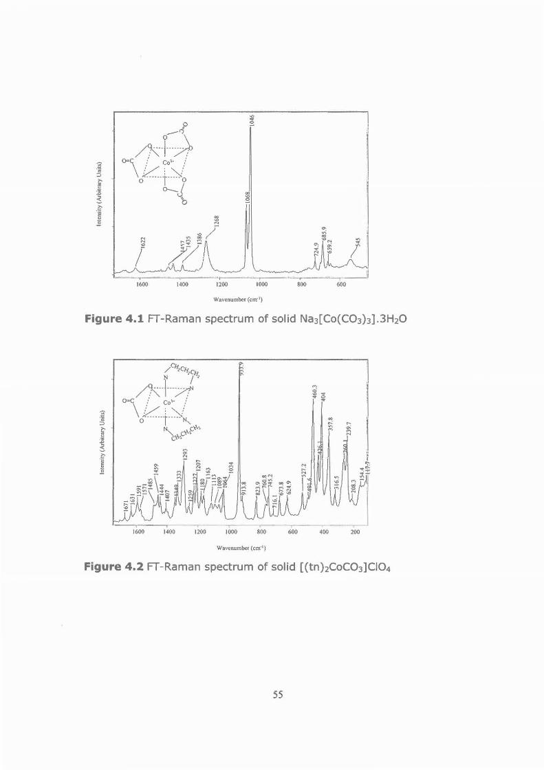
_t /~-r---~
0=\ / Co'' / v.. .. r:_~ .. 0 0
o-J b
IOOO 800 600
Wavenumber (cm·1)
Figure 4.1 FT-Raman spectrum of solid Na3 [Co(C03)J] .3H20
.., g..,. ... C> ..,.
Wavenumber (cm·')
Figure 4.2 FT-Raman spectrum of solid [(tn)iCoC03]CI04
55

...__,.._-..----.---....--..--··-.· ... ~ ........... ~---r------,-·~-1400 1300 1200 1100 1000 900 800 700 600
Wavenumber (cm·1)
Figure 4.3 Ff-Raman spectrum of the solution of 0.1 M cis
[ Co( tn h( H20 hJ ( CI04 h
Reagents and products: It is imperative to analyse FT-Raman spectra of
reactants and products prior to the analysis of spectra for PNPP
hydrolysis; PNP and phosphate are products of the hydrolysis. Since
[(tn)2Co(OH)(H20)]2+ was used to enhance hydrolysis rates, PNPP and
[(tn)zCo(OH)(H20)]2+ are reactants.
Phosphorus compounds have a P-0108, P=0109
•110 and P-0-C (in
aliphatic compounds)30•111 stretching vibrations that can be observed at
1054-910 cm-1, 1350-1150 cm-1 and 1050-970 cm-1 , respectively. FT
Raman spectra of 0.1 M PNPP and 0 . 1 M PNP as shown in Figure 4.4
have both similar and isolated peaks; isolated peaks were used for the
monitoring of PNPP hydrolysis. Because the peaks at 982 and 737 cm-1
(assigned to the phosphate ion108-112) are very weak, only peaks at 1290
and 1266 cm-1 were used to estimate rate constants. As shown in Figure
4.5 below, the FT-Raman spectrum for the [(tn)zCo(OH)(H20)]2+ ion has
56

a strong peak at 935 cm-1, which does not interfere with other peaks of
interest discussed above .
. 0
.0
~ ·c 0.1 M PNP (broken line)
"' ~ !! .0 :e $
1247
>-.'!:< Ill c: ., £
.0 1596 '• j: 1593
1400
!"" .. .. ,,
.. .. .. .. ..
0,,,,0,{)"~ o-0. 1 M PNPP (solid line)
~-- -.----- ·r--1200 1000 800
Wavenumber (cm")
600
Figure 4.4 FT-Raman spectra of solutions of pure 0.1 M PNP and pure
0.1 M PNPP
~ 0.1 M [Co(tnh(Hp)(OH)](CIO.), (dotted line)
.0 0.1 M PNPP (solid line)
products {broken line) such ss PNP
Wavenumber (cm·')
Figure 4.5 FT-Raman spectra of reagents and products in the
[Co(tn)2(0H)(H20)]2+ assisted hydrolysis of PNPP. The
reaction was conducted in a solution of 0.6 M NaN03 .
57

[Co(tn)2(0H)(H20)]2+ assisted hydrolysis of PNPP: This is a Lewis acid
base reaction to form PNP and the Co(tn)iphosphate complex. This
reaction can be monitored by a decrease in the intensity of peaks at
1347 and 1265 cm·1 (PNPP disintegration) and an increase in the
intensity of the peak at 1293 cm·1 (PNP formation)(see Figures 4.5
above, 4.6 and 4.7 below). This trend of change in the intensity of peaks
was observed in all reactions at the pH of 7.3 or uncontrolled pH.
Figure 4.6 shows a 3-dimensional plot of the reaction spectra at the
region 650-1430 cm·1. This region, as mentioned earlier, was used for
the estimation of rate constants, which will be presented later. In
addition to Raman peaks at 1347, 1293 and 1265 cm·1, the region was
extended to 650 cm-1 for the sake of incorporating peaks characterising
[Co(tn)i(OH)(H20)]2+ and Poi-.
As shown in Figure 4. 7, there is a sudden decrease in the Raman peak at
1265 cm·1 whereas the Raman peak at 1347 cm·1 gradually decreases
while a peak at 1293 cm·1 gradually increases. According to Raman
peaks in this figure, the life span of PNPP in the reaction is very short
whereas the formation of PNP increases with time. A possible reason for
this sudden decrease of the Raman peak is the formation of the
Co(tn)iphosphate complex, which is not characterised by a peak at
1265.
58

1293 PNP
935 [ Co(tn)2(H20)(0H)](CIO 4)2
I
/
1.43329e+03cm-1 /
1.24044e+03cm-1 ,,
1 04760e+03<:m-1
" 854 74884cm-1
Figure 4.6 3-dimensional FT-Raman spectra for the
. 00
~ ·c: "
,.. "" .. c: .,
.00 ~
.00
[Co(tn)2(0H)(H20)]2+ assisted hydrolysis of PNPP in the
range 650-1430 cm-1 .
PNP ··~-1 and PNP increases
--.. 1400 1380 1360 1340 1320 1300 1280 1260 1240
Wavenumber (cm·')
Figure 4.7 FT-Raman spectra of [Co(tn)2(0H)(H20)]2+ assisted
hydrolysis of PNPP for three peaks at 1347, 1293 and 1265
cm-1 .
59

4.3.2 Estimation of rate constants for the PNPP
hydrolysis
FT-Raman techniques and the procedure to estimate rate constants and
also to predict mole ratio of PNPP using PLS-MDA were fully discussed in
Chapter 3. The reaction between 0.0267 M [Co(tn)i(OH)(H20)]2+ and
0.0133 M PNPP (molar ratio of 2: 1) will be used as an example to show
plots of regression line, coefficients of multiple determination (R2), mole
ratios and pH.
Figure 4.8 is a summary of PLS-MDA results. To quantify FT-Raman
spectra of this reaction, the kinetic modelling was used to create models
which are represented by the regression line shown in the figure below.
The rate constants were optimised using PLS-MDA and the results are
presented in Figure 4 .9. The rate constant of this reaction was estimated
to be 1.5839 x 10⁻² min-1.

Actual Conoerb.llion ( C1)
Figure 4.8 Plot of Predicted versus Actual concentrations for the molar
ratio 2: 1 of Co(tnhPNPP complex.
0.9729 c
0.9715
0.9701 .. v= -411.o1')("+13.02x+ 0.8695
R2 = 0.9994 0.9687 +----.------T----r"
00128 00146 0.0164 O.o182
k (min.1)
Figure 4.9 Plots of coefficient of multiple determination (R2) versus
first order rate constant (k1,opt) for the molar ratio 2: 1 of
Co(tn)iPNPP complex.
Figure 4.10 below shows plots of concentrations and pH values. In this
reaction, pH was initiated at 7. 3 but was not kept constant throughout.
When [Co(tn)2(H20)(0H)](CI04)2 and PNPP were mixed, the monitored
61

pH values increased to a maximum and then gradually decreased. This
phenomenon was explained earlier using Ff-Raman spectra (refer to
section 4 .3 .1). The sudden increase of pH to the maximum is known as
the short induction period 12; in this work, induction period was observed
at pH 8.13 in 8.00 minutes for molar ratio of 2: 1.
According to Figure 4.10, the plot of mole ratio and time is correlated by
an exponential function. The pH values of the solution after the induction
period started decreasing as the number of moles of PNPP was
decreasing. The Co(tn)iPNPP complex in basic media disintegrated to
form acidic PNP. Prior to monitoring of these reactions, pH of
[Co(tn)i(H20)(0H)](CI04h and PNPP were measured and were found to
be 2.84 (due to HCI04 used in the preparation) and 8.20, respectively. A
reason for the pH increase will be discussed later.
0.8
0 0.6 ~ Q)
~ E 0.4
0.2
0 0 41 83
time (min)
125 167
8.14
7.93
1.12 :a
7.51
Figure 4.10 Plots of mole ratio (left ordinate) and pH (right ordinate)
versus time for the ratio 2: 1 of Co(tn)iPNPP complex.
62

Table 4.2 shows rate constants of PNPP hydrolysis at specific pH
conditions (more information on rate constants can be found in Appendix
2; the rate constants in Table 4.2 were estimated using GRAMS32, which
is confirmed by the Unscrambler results found in Appendix 3). The rate
constants for the hydrolysis of PNPP are plotted in Figure 4.11. The rate
constant (k1) for pathway 1 or 2 are interpreted using equations already
described.
63

Table 4.2 First order rate constants rate (k1) of the PNPP hydrolysis
with respect to PNPP estimated using FT-Raman techniques
and PLS-MDA (Refer to Equations 4.2 and 4.3, and Table
4.1).
Reacti on monitored a t pH 7 .30
Limits [M)o [L]o [M]/[T) kl
0.0200 0 .0 200 0.5000 9 .8935E-03
0 .0240 0 .0160 0 .6000 8 .3251E-03
0 .0267 0.0133 0.6675 1.3691 E-02
0 .0286 0.0144 0 .6651 1.6 158E-02
0 .0300 0.0100 0 .7500 8.6825E-03
0 .0267 0 .0133 0 .6675 l.0664E-02
0 .0080 0.0320 0.2000 5. 1392E-03
0 .0133 0.0267 0 .3325 8.2326E-03
0 .0267 0 .0133 0 .6675 8.8986E-03
0.0320 0.0080 0.8000 7.1366E-D3
0 .0100 0 .0300 0.2500 6 .9929E-03
0 .0200 0 .0200 0.5000 8.5980E-03
0.0300 0.0100 0.7500 1.2700E-02
Reaction m oni to red from pH 7 .3 o
Limits [M)o [L] 0 [M]/[T] k1
0.0100 0 .0300 0.2500 2 .6688E-02
0 .0120 0 .0280 0 .3000 2 .9978E-02
0 .0160 0 .0240 0 .4000 1.8316E-02
0 .0200 0 .0200 0.5000 2 .2582E-02
0 .0240 0 .0160 0 .6000 1.9963E-02
0 .0267 0 .0133 0 .6675 1.5839E-02
64

3.SE-02
3.0E-02
2.SE-02
~ ... 'c: 2.0E-02 E ..._, -~
1.SE-02
1 .0E-02
5 .0E-03
0 .OE+OO 0 .0
y = -0.026x + 0.034
OpH 7.30 ~pH monitaed
)(0
0 0
0 y = 0.0085x + O.oo.ta
0.2 0.4 0.6 0.8
[M]/[T]
1.0
Figure 4.11 A plot of k1 versus mole fraction of M for the hydrolysis
reactions.
The discussion below is categorised into two sections; firstly the
discussion focuses on the reaction scheme during the induction period
and then the reaction scheme disintegration periods.
1 During the induction period
Figure 4.7 (above) : Induction period is the period where the
formation of PNP is very slow, which later accelerate. Sudden
decrease of a Raman peak at 1265 cm·1 (a peak characterising
PNPP) can reveal a very short life span of PNPP in the reaction,
which can be attributed to the formation of the Co(tn)iPNPP
complex. Although the spectrum of interest (the second spectrum)
65

is not clearly shown in the figure because of other spectra, it was
recorded after about 5 to 6 minutes from the start of the reaction.
This information will be combined with the one that will be
discussed below.
Figure 4.10 (above): Mixing [Co(tn)i(OH)(H20)](CI04)2 and PNPP
at pH 7.30 caused the pH of the hydrolysis to increase suddenly to
a maximum of 8.16 within 5 minutes (average pH and time for
several reactions). According to the pH measurement in this work,
the formation of the Co(tn)iPNPP complex causes the reaction
mixture to be basic, that is, releasing hydroxyl ion.
Therefore,
trans cis
and/or
RO Q \ ,.....O-c /""'\ 0-P. I~"\ '-c..: / \ HO v Go" 0 (H)
(~~ Figure 4.12 The hydrolysis scheme13 for the formation of the
Co(tn)iPNPP complex, where PNPP = P04R2- (charges are
mostly omitted).
66

2 During the disintegration period
Figure 4.7 (above): The disintegration period is a period where
PNP is released from the complex formed above. The Raman peak
at 1293 cm·1 (a peak characterising PNP) increases gradually as
the hydrolysis proceeds. In this case, the Co(tn)iPNPP complex
disintegrates to form PNP and Co(tn)iphosphate complex.
Figure 4.10 (above): The Co(tn)2PNPP at the maximum pH of 8.16
for the induction period of roughly 5 minutes starts to disintegrate
into acidic PNP and the Co(tn)iphosphate complex. As more
02NC5H40-H+ is formed, more H+ ions are contributed to the
reaction. Hence the hydrolysis pH gradually decreases.
RO O \ /
G /o-P,o Geo,
OH (H)
mono-coordinated species
! cobalt-monomer
RO Q '/o-c QC /O-~ Hd ~ Co'oH 0 (H)
(H) bi-coordinated species
l
cobalt-dimer
Figure 4.13 Hydrolysis scheme13 for the disintegration of Co(tn)2PNPP
complex to form ROH (PNP), in this work R = p-nitrophenyl
(charges are mostly omitted).
67

4.3.3 Correlations between rate constants and
hydrolysis pathways
According to the above discussions, the hydrolysis of PNPP in this work
does not follow pathway 1 because of the existence of a short induction
period, which is possibly caused by the formation of the Co(tn)iPNPP
complex. In this section, conditions for pathway 2 (from the theory,
section 4.1.2) will be discussed.
Condition 1: The first order rate constant (k1) for each hydrolysis was
estimated using the FT-Raman techniques and PLS-MDA (Table 4.3); k1
= k3 (from Equation 4.5, that is, ML ~ P). The rate constants from the
estimated data are plotted in Figure 4.14, which is similar to Figure 4.11
above. The graph in Figure 4.11 shows plots of k1 as a function of molar
concentration of M. When points in the graph are extrapolated with a
straight line, the line for the hydrolysis where pH starts at 7 .3 has a
negative slope; while the line for the hydrolysis at constant pH 7.3 has a
positive slope. For the PNPP hydrolysis at pH 7.3, k1 (= kJ) is scattered
in the range 0.6 to 0.8 min-1. The 0/o Error in the table is calculated using
the following equation below:
k (A)-k (B) 0/o Error= 1 k1 (A) x100°/o (4.17)
where
ki(A) is a first order rate constant estimated using the kinetic
modelling (data in Table 4.2), and
k1(B) is a first order rate constant calculated using straight line
equations found in Figure 4.14.
68

Table 4.3 Rate constants for PNPP hydrolysis
<eaction monitored at pH 7.30
Limits [M]o [L]o [M]/[T] k 1 (A) k1 (B) % Error
0.0200 0.0200 0.5000 9.8935E-03 9.0560E-J3 8.47
0.0240 0.0160 0.6000 8.3251E-03 9.9072E-J3 19.00
0.0267 0.0133 0 .6675 1.3691E-02 1.0482E-J2 23.44
0.0286 0 .0144 0.6651 1.6158E-02 1.0886E-J2 32.63
0.0300 0.0100 0.7500 8.6825E-03 l.1184E-J2 28.81
0.0267 0.0133 0.6675 1.0664E-02 1.0482E-J2 1.71
0.0080 0.0320 0.2000 5.1392E-03 6.5024E-J3 26.53
0.0133 0 .0267 0.3325 8.2326E-03 7.6302E-J3 7.32
0.0267 0.0133 0.6675 8.8986E-03 1.0482E-J2 17.79
0.0320 0.0080 0.8000 7.1366E-03 1.1610E-J2 62.68
0.0100 0.0300 0.2500 6.9929E-03 6.92BOE-J3 0.93
0.0200 0.0200 0.5000 8.59BOE-03 9.0560E-J3 5.33
0.0300 0.0100 0.7500 1.2700E-02 1.1184E-J2 11.94
<eaction monitored from pH 7 .30
Limits [M]o [L]o [M]/[T] k 1 (A) k1 (B) % Error
0.0100 0.0300 0.2500 2.6688E-02 2.7497E-02 3.03
0.0120 0.0280 0.3000 2.9978E-02 2 .6196E-02 12.61
0.0160 0.0240 0.4000 1.8316E-02 2.359SE-02 28.82
0.0200 0.0200 0.5000 2.2582E-02 2.0994E-02 7 .03
0.0240 0.0160 0.6000 1.9963E-02 1.8393E-02 7.87
0.0267 0.0133 0.6675 1.5839E-02 1.6637E-02 5.04
69

3.SE-02
3 .0E-02
2.SE-02
-... ' c: 2.0E-02 E
......... <{ 1.SE-02 .._, ... ~
1.0E-02
5.0E-03
O.OE+OO 0.000
o pH 7.30 __!_pH monitored
0 0
o y = 0.2128x + 0.0048
0.010 0.020
[M]o
0.030 0.040
Figure 4.14 A plot of k1 versus concentration of M for hydrolysis
reactions.
Condition 2: It is an alternative to condition 1 discussed above. In this
part only Equation 4.6 (that is, ML + M ~ P) is the rate determining
step, therefore, k1(A) = k/ (from Equation 4.11). Since ki(A) is the first
order rate constant, the second order rate constant k4 = ki(A)/[M]
(Figure 4.15) . k4 for the PNPP hydrolysis at all pH conditions decreases
with a decrease in [Co(tn)i(OH)(H20)]2+, but the decrease is steeper for
the hydrolysis where pH was monitored as shown in Figure 4.15 below.
70

2.SE+OO
.......... ~c 2 .0E+OO E ~ ......, ,....., 1.SE+OO ::E .......... .......... .......... <(
~ 1.0E+OO
5.0E-01
~ o pH 7.30 [ ::K pH monitored
0
o.oe+oo~.~~~~~~~~~~~~~~~~~~~~
0.000 0.010 0 .020
[M]o
0.030 0 .040
Figure 4.15 A plot of ki/[M] versus concentration of M for hydrolysis
reactions.
Condition 3: It is the second alternative for condition 1, it is actually the
combination of conditions 1 and 2 (Equations 4.5 and 4.6). k1(A) = k* is
pseudo first order and it is represented by the straight lines (Equation
4.18 and 4 .19) from Figure 4.14.
For the PNPP hydrolysis where the pH was not kept constant,
k1 (A)= -0.6503[M]+ 0.034 (4.18)
71

And for the hydrolysis at pH 7.3,
k 1(A) = 0.2128[M]+0.0048 (4.19)
Therefore, it was possible to estimate different rate constants of PNPP
hydrolysis using FT-Raman techniques and PLS-MDA. Hydrolysis rates
were not estimated because they require the equilibrium constant, which
was not determined in this work. It was possible to extract the
equilibrium constant from literature, but it was only the aim of this work
to estimate rate constants using the described techniques.
4.4 Conclusions
1. FT-Raman spectra were successfully used to analyse cobalt(III)
complexes. Replacements of groups in cobalt(III) complexes were
identified by the disappearing and appearing of spectral peaks
during hydrolysis. The presence of [Co(tn)2(0H)(H20)]2+ ions
during the PNPP hydrolysis was identified by a peak at 935 cm-1,
which is assigned to CH2 rocking vibration of tn.
2. The Raman spectrum of [Co(tn)i(OH)(H20)]2+ has a peak 935 cm-
1, PNP has a peak at 1266 cm-1 and PNP has a peak at 1290 cm-1,
which overlap. The last two mentioned peaks were successfully
utilised to quantify the hydrolysis of PNPP because the peak at
1266 cm-1 decreases as PNPP phosphate reacts while the peak at
1290 cm-1 increases as PNP is formed.
3. The hydrolysis of p-nitrophenylphosphate was conducted under
two different conditions viz. at constant pH of 7.3 and an initial pH
72

of 7.3, which gave a graph with two different trends of rate
constants. The outcome shows that first order rate constants with
respect to PNPP hydrolysis are higher when the pH is not
maintained throughout.
4. pH values of reactions with a changing pH from 7 .3 were
monitored and their change
immediately after combining
cobalt(III) perchlorate and
confirmed the induction period
bis-(1,3-diaminopropane)diaqua-
p-nitrophenylphosphate. This
phenomenon was observed by an increase of pH values from 7.3
to maximum values shown earlier (Figure 4.12), which is the
coordination of the ligand (p-nitrophenylphosphate) to the metal
complex.
73

CHAPTER 5
Cone I usions and future investigations
5.1 Conclusions
FT-Raman techniques (a combination of online sampling system at the
Raman spectrometer and kinetic modelling methods), together with the
multivariate data analysis method, were successfully used to re-estimate
rate constants of the hydrochloric acid catalysed inversion of sucrose.
Then these techniques were used to estimate rate constants of
cobalt(III) assisted hydrolysis of p-nitrophenyl-phosphate.
The online sampling system was achieved by making a loop that
circulates the solution from the reaction vessel to the sampling
compartment of the FT-Raman spectrometer, where it was scanned. The
sample solution in the reaction vessel was stirred by the magnetic stirrer
while a portion of the reaction solution was circulated by the peristaltic
pump. This method was successfully used to conduct real time
monitoring of reactions.
Though FT-Raman spectra of reaction solutions have several weak and
overlapping peaks, in particular for the acid catalysed inversion of
sucrose, changes of spectral peaks in general were monitored using
multivariate data analysis. Considering the inversion of sucrose and the
hydrolysis of cobalt(III) nitrophenylphosphate, it was possible to monitor
a decrease in the intensity of the Raman peaks of reagent molecules and
also the increase in the intensity of Raman peaks as products formed.
74

PLS results for the calibration and the kinetic modelling of the acid
catalysed inversion of sucrose are comparable. The Raman spectra of
sucrose, fructose and glucose, and rate constants for the inversion of
sucrose were found to be comparable to the values reported in the
literature. For the hydrolysis of cobalt(III) nitrophenylphosphate, it was
found that rate constants where the pH is maintained at 7.30 gave
results which differ from those where the pH is started at 7.30 and
allowed to change during the reaction. The average rate constant for a
2: 1 ([Co(tnh(OH)(H20)]2+:PNPP) was found to be approximately 3 x 10⁴
times the unassisted PNPP hydrolysis rate reported in the literature.
5.2 Future investigations
All reactions for the hydrolysis of cobalt(III) nitrophenylphosphate were
carried-out in 8-10 x 10-3 M because their Raman peaks at lower
concentrations such as 10-6 M were very weak. Real time monitoring of
reactions at lower concentrations of reagents can be achieved by
enhancing spectral peaks with non-reacting silver or gold colloids. The
surface enhancement is possible when the Raman effect is close to the
rough metal surface.
It is difficult to assign spectral peaks and to characterise the hydrolysis
of cobalt(III) nitrophenylphosphate because theoretical studies for
vibrational modes of p-nitrophenylphosphate and bis-(1,3-
diaminopropane)diaquacobalt(III) perchlorate have not been done yet.
Future uses of chemical modelling for these compounds or complexes
and reactions would be an advantage to interpret experimental evidence.
75

APPENDICES
Appendix 1: Crystallographic data for [Co(tn)iC03]CIQ4
Table I. Crystal data and structure refinement for SPO I.
Identification code spOl_abs
Empirical formula
Formula weight
Temperature
Wavelength
Crystal system
Space group
Unit cell dimensions
Volume
z Density (calculated)
Absorption coefficient
F(OOO)
Crystal size
Theta range for data collection
Index ranges
Reflections collected
Independent reflections
Completeness to theta= 25.00°
Absorption correction
Max. and min. transmission
Refinement method
Data I restraints I parameters
Goodness-of-fit on F2
Final R indices [1>2sigma(I))
R indices (all data)
Extinction coefficient
Largest diff. peak and hole
C1 H20 Cl Co N4 01
366.65
293(2) K
o.71073 A
Monoclinic
P 21/c
a= 9.5347(5) A
b = 13.2166(7) A
c = I 2.0977(7) A
1415.75(13) A3
4
1.720 Mg/m3
1.437 mm-1
760
0.42 x 0.41 x 0.16 mm3
2.77 to 26.49°.
b= 111.7730(10)0•
g = 90°.
- 11 <='h<=9, -15<=k<=l 2, -8<=1<=15
7336
2670 [R(int) = 0.0205]
99.5 %
Semi-empirical from equivalents
0.795 and 0.583
Full-matrix least-squares on F2
2670 I 0 I 218
1.083
RI = 0 .0334, wR2 = 0.0871
RI= 0 .0354, wR2 = 0.0894
0
0.457 and -0.358 e.A-3
76

Appendix 2: PLS-MDA results for PNPP hydrolysis using GRAMS32. Below are results of twenty one samples for the modelling of the reaction.
Sample 1 k PC Prediction Bias PRESS R2 RMSD k 1,opt
0.00556 -0.00032 0.03749 0.93552 0.03273 0.00989
0.00695 1 -0.00032 0.04956 0.93755 0.03763
0.00833 1 -0.00028 0.06125 0.93879 0.04183
0.00972 1 -0.00023 0.07260 0.93925 0.04554
0.01111 -0.00016 0.08378 0.93894 0.04893
0.01250 -0.00008 0.09502 0.93787 0.05210
0.01389 1 0.00001 0.10652 0.93607 0.05517
0.01528 0.00010 0.11845 0.93355 0.05818
0.01667 0.00020 0.13092 0.93036 0.06116
Sample 2 k PC Prediction Bias PRESS R2 RMSD k1 ,opt
0.01110 0.00014 0.05940 0.95688 0.04120 0.01369
0.01180 0.00019 0.06214 0.95751 0.04213
0.01250 1 0.00024 0.06486 0.95794 0.04305
0.01320 0.00029 0.06762 0.95817 0.04395
0.01390 0.00034 0.07045 0.95820 0.04486
0.01460 1 0.00040 0.07339 0.95804 0.04579
0.01530 0.00046 0.07647 0.95769 0.04674
0.01600 0.00051 0.07972 0.95716 0.04773
0.01670 0.00057 0.08316 0.95644 0.04874
Sample 3 k PC Prediction Bias PRESS R2 RMSD k 1,opl
0.00555 0.00118 0.03515 0.94677 0.03169 0.00868
0.00642 0.00136 0.04259 0.94768 0.03488
0.00729 1 0.00153 0.05000 0.94830 0.03780
0.00816 1 0.001 71 0.05737 0.94861 0.04049
0.00903 0.00188 0.06471 0.94864 0.04300
0.00990 0.00205 0.07203 0.94837 0.04537
0.01076 1 0.00221 0.07938 0.94782 0.04762
0.01163 1 0.00237 0.08680 0.94699 0.04980
0.01250 0.00252 0.09431 0.94588 0.05191
77

Sample4 k PC Prediction Bias PRESS R2 RMSD k,,opl
0.00100 0.00007 0.00154 0.94883 0.00663 0.00833
0.00263 0.00020 0.00825 0.95305 0.01535
0.00425 1 0.00036 0.01715 0.95621 0.02214
0.00588 1 0.00055 0.02663 0.95830 0.02758
0.00750 1 0.00074 0.03620 0.95932 0.03216
0.00913 0.00095 0.04595 0.95930 0.03623
0.01075 0.00115 0.05617 0.95824 0.04006
0 .01238 0.00136 0.06720 0.95618 0.04382
0.01400 1 0.00156 0.07930 0.95315 0.04760
Sample 5 k PC Prediction Bias PRESS R2 RMSD k1.op1
0.00100 0.00006 0.00235 0.92556 0.00820 0.00274
0.00141 0.00009 0.00444 0.92583 0.01126
0.00181 1 0.00013 0.00705 0.92603 0.01419
0.00222 1 0.00016 0.01010 0.92616 0.01699
0.00262 0.00020 0.01354 0.92621 0.01967
0.00303 0.00023 0.01732 0.92620 0.02224
0.00344 1 0.00027 0.02138 0.92611 0.02472
0.00384 1 0.00031 0.02569 0.92596 0.02709
0.00425 0.00035 0.03023 0.92573 0.02939
Sample6 k PC Prediction Bias PRESS R2 RMSD k1 ,opt
0.00830 2 0.00222 0.07837 0.92592 0.04732 0.01066
0.00900 2 0.00233 0.08602 0.92601 0.04957
0.00970 2 0.00242 0.09337 0.92607 0.05165
0.01040 2 0.00250 0.10041 0.92609 0.05356
0.01110 2 0.00256 0.10709 0.92608 0.05531
0.01180 2 0.00261 0.11340 0.92604 0.05692
0.01250 2 0.00264 0.11934 0.92598 0.05839
0.01320 2 0.00265 0.12489 0.92590 0 .05973
0.01390 2 0.00264 0.13005 0.92579 0.06096
78

Sample 7 k PC Prediction Bias PRESS R2 RMSD k1,opl
0.00110 1 0.00011 0.00276 0.92823 0.00888 0.00253
0.00141 1 0.00015 0.00439 0.92839 0.01121
0.00173 1 0.00018 0.00633 0.92852 0.01345
0.00204 0.00021 0.00855 0.92860 0.01563
0.00235 0.00025 0.01100 0.92864 0.01773
0.00267 0.00028 0.01367 0.92864 0.01976
0.00298 0.00032 0.01653 0.92861 0.02173
0.00329 0.00036 0.01956 0.92853 0.02364
0.00360 1 0.00039 0.02271 0.92841 0.02547
Samples k PC Prediction Bias PRESS R2 RMSD k1,opl
0.00582 2 -0.00014 0.01976 0.96753 0.02376 0.00714
0.00621 2 -0.00013 0.02153 0.96777 0.02480
0.00661 2 -0.00013 0.02332 0.96792 0.02582
0.00701 2 -0.00012 0.02516 0.96799 0.02681
0.00741 2 -0.00012 0.02704 0.96798 0.02779
0.00781 2 -0.00011 0.02897 0.96788 0.02877
0.00820 2 -0.00010 0.03097 0.96769 0.02974
0.00860 2 -0.00009 0.03303 0.96742 0.03072
0.00900 2 -0.00007 0.03519 0.96707 0.03171
Samples k PC Prediction Bias PRESS R2 RMSD kl.opt
0.00300 2 0.00050 0.04606 0.78459 0.03628 0.00514
0.00340 2 0.00055 0.05664 0.78487 0.04023
0.00380 2 0.00059 0.06780 0.78510 0.04401
0.00419 2 0.00063 0.07941 0.78527 0.04763
0.00459 2 0.00066 0.09139 0.78538 0.05110
0.00499 2 0.00070 0.10366 0.78543 0.05442
0.00539 2 0.00072 0.11614 0.78543 0.05760
0.00579 2 0.00075 0.12877 0.78536 0.06066
0.00618 2 0.00077 0.14149 0.78524 0.06358
79
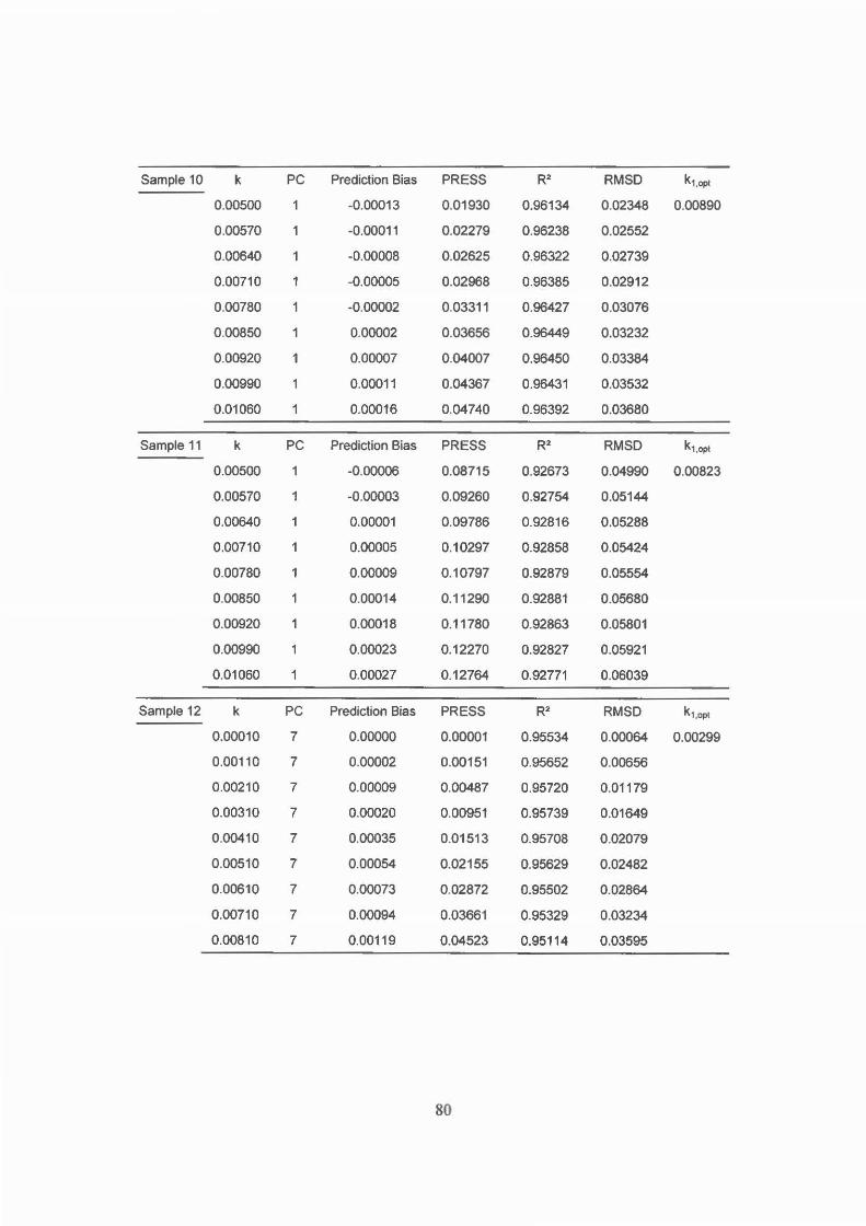
Sample 10 k PC Prediction Bias PRESS R2 RMSO k1,opt
0.00500 -0.00013 0,01930 0.96134 0.02348 0.00890
0.00570 1 -0.00011 0.02279 0.96238 0.02552
0.00640 1 -0.00008 0.02625 0.96322 0.02739
0.00710 1 -0.00005 0.02968 0.96385 0.02912
0.00780 -0.00002 0.03311 0.96427 0.03076
0.00850 1 0.00002 0.03656 0.96449 0.03232
0.00920 1 0.00007 0.04007 0.96450 0.03384
0.00990 0.00011 0.04367 0.96431 0.03532
0.01060 1 0.00016 0.04740 0.96392 0.03680
Sample 11 k PC Prediction Bias PRESS R2 RMSO k,,opt
0.00500 1 -0.00006 0.08715 0.92673 0.04990 0.00823
0.00570 1 -0.00003 0.09260 0.92754 0.05144
0.00640 0.00001 0.09786 0.92816 0.05288
0.00710 1 0.00005 0.10297 0.92858 0.05424
0.00780 1 0.00009 0.10797 0.92879 0.05554
0.00850 0.00014 0.11290 0.92881 0.05680
0.00920 1 0.00018 0.11780 0.92863 0.05801
0.00990 0.00023 0.12270 0.92827 0.05921
0.01060 1 0.00027 0.12764 0.92771 0.06039
Sample 12 k PC Prediction Bias PRESS R2 RMSO k1,opt
0.00010 7 0.00000 0.00001 0.95534 0.00064 0.00299
0.00110 7 0.00002 0.00151 0.95652 0.00656
0.00210 7 0.00009 0.00487 0.95720 0.01179
0.00310 7 0.00020 0.00951 0.95739 0.01649
0.00410 7 0.00035 0.01513 0.95708 0.02079
0.00510 7 0.00054 0.02155 0.95629 0.02482
0.00610 7 0.00073 0.02872 0.95502 0.02864
0.00710 7 0.00094 0.03661 0.95329 0.03234
0.00810 7 0.00119 0.04523 0.95114 0.03595
80

Sample 13 k PC Prediction Bias PRESS RZ RMSD k1,opt
0.00950 0.00039 0.20802 0.82961 0.07709 0.01270
0.01037 0.00045 0.22736 0.83060 0.08060
0.01124 1 0.00050 0.24566 0.83127 0.08378
0.01211 1 0.00056 0.26296 0.83163 0.08668
0.01298 0.00062 0.27930 0.83168 0.08933
0.01385 0.00068 0.29475 0.83142 0.09177
0.01471 1 0.00074 0.30938 0.83086 0.09402
0.01558 1 0.00080 0.32327 0.83001 0.09611
0.01645 0.00086 0.33648 0.82888 0.09805
Sample 14 k PC Prediction Bias PRESS RZ RMSD k1,opt
0.00050 1 0.00002 0.00073 0.91099 0.00456 0.00699
0.00170 0.00009 0.00719 0.91363 0.01434
0.00290 0.00018 0.01806 0.91574 0.02271
0.00410 1 0.00028 0.03137 0.91731 0.02994
0.00530 1 0.00040 0.04591 0.91833 0.03622
0.00650 0.00052 0.06097 0.91882 0.04174
0.00770 0.00066 0.07614 0.91877 0.04664
0.00890 1 0.00079 0.09125 0.91818 0.05106
0.01010 0.00093 0.10623 0.91707 0.05509
Sample 15 k PC Prediction Bias PRESS RZ RMSD k 1,opt
0.00500 1 0.00014 0.00921 0.98167 0.01623 0.00860
0.00600 1 0.00021 0.01119 0.98301 0.01788
0.00700 0.00028 0.01312 0.98391 0.01936
0.00800 0.00036 0.01514 0.98437 0.02080
0.00900 1 0.00044 0.01739 0.98440 0.02229
0.01000 1 0.00053 0.02001 0.98401 0.02391
0.01100 0.00062 0.02313 0.98320 0.02570
0.01200 0.00072 0.02684 0.98197 0.02769
0.01300 0.00081 0.03125 0.98034 0.02988
8l

Sample 16 k PC Prediction Bias PRESS R2 RMSD k1.opt
0.01550 2 0.00008 0.06853 0.98230 0.03408 0.01832
0.01620 2 0.00012 0.06746 0.98270 0.03381
0.01690 2 0.00016 0.06666 0.98299 0.03361
0.01760 2 0.00020 0.06617 0.98316 0.03349
0.01830 2 0.00023 0.06601 0.98322 0.03345
0.01900 2 0.00026 0.06621 0.98316 0.03350
0.01970 2 0.00029 0.06676 0.98299 0.03364
0.02040 2 0.00031 0.06768 0.98271 0.03387
0.02110 2 0.00033 0.06894 0.98232 0.03418
Sample 17 k PC Prediction Bias PRESS R2 RMSD k1,opl
0.01970 1 -0.00007 0.06016 0.98213 0.03221 0.02258
0.02040 -0.00002 0.05576 0.98333 0.03101
0.02110 0.00003 0.05254 0.98417 0.03010
0.02180 1 0.00008 0.05044 0.98467 0.02949
0.02250 0.00012 0.04939 0.98485 0.02918
0.02320 0.00017 0.04935 0.98470 0.02917
0.02390 1 0.00021 0.05023 0.98426 0.02943
0.02460 1 0.00025 0.05196 0.98352 0.02993
0.02530 0.00030 0.05447 0.98250 0.03065
Sample 18 k PC Prediction Bias PRESS R2 RMSD k1,0pl
0.01280 -0.00003 0.11258 0.96875 0.04368 0.01584
0.01350 1 0.00002 0.10877 0.97035 0.04294
0.01420 1 0.00008 0.10603 0.97151 0.04239
0.01490 0.00013 0.10447 0.97224 0.04208
0.01560 0.00018 0.10415 0.97256 0.04201
0.01630 1 0.00024 0.10508 0.97247 0.04220
0.01700 0.00029 0.10728 0.97199 0.04264
O.Q1770 0.00034 0.11070 0.97114 0.04332
0.01840 1 0.00039 0.11531 0.96992 0.04421
82

Sample 19 k PC Prediction Bias PRESS R2 RMSD k1 ,opl
0.01750 1 -0.00002 0.04446 0.98822 0.02769 0.01996
0.01820 0.00003 0.04052 0.98929 0.02643
0.01890 0.00009 0.03792 0.98998 0.02557
0.01960 1 0.00014 0.03663 0.99031 0.02513
0.02030 0.00020 0.03660 0.99029 0.02512
0.02100 1 0.00025 0.03778 0.98994 0.02552
0.02170 1 0.00030 0.04011 0.98927 0.02630
0.02240 1 0.00035 0.04351 0.98828 0.02739
0.02310 0.00040 0.04792 0.98701 0.02874
Sample20 k PC Prediction Bias PRESS R2 RMSD k1,opt
0.02700 1 0.00039 0.13567 0.96173 0.04795 0.02998
0.02770 0.00043 0.13103 0.96269 0.04713
0.02840 1 0.00048 0.12739 0.96337 0.04647
0.02910 0.00052 0.12468 0.96379 0.04597
0.02980 0.00056 0.12283 0.96395 0.04563
0.03050 1 0.00060 0.12180 0.96387 0.04544
0.03120 0.00064 0.12151 0.96356 0.04538
0.03190 0.00068 0.12193 0.96303 0.04546
0.03260 1 0.00072 0.12298 0.96228 0.04566
Sample21 k PC Prediction Bias PRESS R2 RMSD k1.opl
0.02400 0.00032 0.17646 0.95446 0.05423 0.02669
0.02470 0.00036 0.17222 0.95523 0.05358
0.02540 0.00040 0.16887 0.95574 0.05305
0.02610 1 0.00044 0.16636 0.95603 0.05266
0.02680 0.00048 0.16464 0.95608 0.05238
0.02750 0.00052 0.16368 0.95593 0.05223
0.02820 1 0.00056 0.16341 0.95556 0.05219
0.02890 0.00059 0.16381 0.95499 0.05225
0.02960 0.00063 0.16482 0.95423 0.05241
83

Appendix 3 The first order rate constants for selective PNPP hydrolysis to validate the results obtained using GRAMS32 software package. The results of GRAMS32 are comparable to one of the Unscrambler software package.
k (min"1)
[M]o [L]o [M]J[T]o GRAMS32 UNSCRAMBLER
0 .0200 0 .0200 0 .5000 9.8935E- D3 9.8571E-03
0.0240 0.0160 0 .6000 8.325 lE-03 8.5337E-03
0 .0267 0 .0133 0 .6675 1.369 lE-02 1.3704E-02
0.0286 0 .0144 0 .715 l.6158E-02 1.6670E-02
0 .0300 0 .0100 0.7500 B.6825E-03 9 .1971E-03
0.0267 0 .0133 0.6675 1.5839E-02 l.596SE-02
84

REFERENCES
1 F. Tafesse and N. C. Deppa, Ecotoxicol. Environ. Saf., 2004, 260-
266.
2 V. H. Freed, C. T. Chiou and D. W. Schmedding, J. Agric. Food
Chem., 1979, 27(4), 706-708.
3 Organophosphate insecticides Chapter 4, Oregon State University,
http://npic.orst.edu/RMPP/rmpp ch4.pdf, 15 November 2006.
4 A. A. Wang, A. Mulchandani and W. Chen, Appl. Environ.
Microbial., 2002, 68(4), 1684-1689.
5 L. Gharahbaghian and T. Bey, International Journal of disaster
medicine, 2003, 2, 103-108.
6 A. D. F Toy and E. N. Walsh, Phosphorus Chemistry in Everyday
Living, American Chemical Society, 1987.
7 E. J. Griffith, A. Beeton, J. M. Spencer and D. T. Mitchell,
Environmental Phosphorus Handbook, John Wiley & Sons, Inc.,
1973.
8 Y. Mndubu, MSc Dissertation: Comparative study for iron mediated
hydrolysis of 4-nitrophenyl phosphate in cationic and anionic
microemulsion media., University of South Africa, 2005.
85

9 N. C. Deepa, MSc Dissertation: Metal ion containing
microemulsions for the hydrolysis of 4-nitropheny/ phosphate: a
model for decontamination of chemical warfare like
organophosphate, Chemistry Department, University of Transkei,
Private Bag Xl, UNITRA, 2002, 5100.
10 D. Lee, S. Lee, G. H. Seong, J. Choo, E. K. Lee, D. G. Gweon and
S. Lee, Appl. Spectrosc., 2006, 60(4), 373-377.
11 P. K. Grzyska, P. G. Czyryca, J. Purcell and A. C. Hengge, J. Am.
Chem. Soc., 2003, 125, 13106-13111.
12 0. I. Guliy, O. V. Ignatov, 0. E. Makarov and V. V. Ignatov,
Biosens. Bioe/ectron., 2003, 18, 1005-1013.
13 G. H. Rawji, M. Yamada, N. P. Sadler, R. M. Milburn, Jnorg. Chim.
Acta. , 2000, 303(2), 168-174.
14 K. Sorensen-Stowell and A. C. Hengge, J. Org. Chem., 2005, 70,
4805-4809.
15 R. L. Fanshawe, A. G. Blackman and C. R. Clark, Jnorg. Chim.
Acta., 2003, 342, 114-124.
16 D. R. Jones, L. F. Lindoy and A. M. Sargeson, J. Am. Chem. Soc.,
1983, 105, 7327-7336.
17 P. W. A. Hubner and R. M. Milburn, lnorg. Chem., 1980, 19, 1267-
1272.
18 F. Tafesse, Int. J. Mo/. Sci., 2003, 4, 362-370.
86

19 J. Rawlings, W. W. Cleland and A. C. Hengge, J . Inorg. Biochem.,
2003, 93, 61-65.
20 P. K. Grzyska, P. G. Czyryca, J. Golightly, K. Small, P. Larsen, R.
H. Hoff and A. C. Hengge, J. Org. Chem., 2002, 67, 1214-1220.
21 S. G. Srivatsan and S. Verma, Chem. Commun., 2000, 515-516.
22 F. Tafesse, Inorg. Chim. Acta, 1998, 269, 287-291.
23 F. Tafesse, Analyst, 1997, 122, 293-295.
24 J. Rawlings, A. C. Hengge and W. W. Cleland, J. Am. Chem. Soc.,
1997, 119, 542-549.
25 A. C. Hengge, W. A. Edens and H. Elsing, J. Am. Chem. Soc.,
1994, 116, 5045-5049.
26 I. R. Jonassen, S. F. Lincoln and D. R. Stranks, Austral. J. Chem.,
1970, 23, 2267.
27 H. F Bauer and W. C. Drinkard, J. Am. Chem. Soc., 82, 1960,
5031-5032.
28 S. Armenta, G. Quintas, S. Garrigues and M. de la Guardia, Trends
Anal. Chem., 2005, 24(8), 772-780.
29 S. G. Skoulika, C. A. Georgiou and M. G Polissiou, Appl.
Spectrosc., 1999, 53(11), 1470-1474.
87

30 S. G. Skoulika and C. A. Georgiou, Appl. Spectrosc., 2000, 54(5),
747-752.
31 N. Taranenko, J. P. Alarie, D. L. Stokes and T. Vo-Dinh, J. Raman
Spectrosc., 1996, 27, 379-384.
32 P.A. Tanner and K. H. Leung, Appl. Spectrosc., 1996, 50(5), 565-
571.
33 D. Aslanian, P. Grof, F. Renault and P. Masson, Biochim. Biophys.
Acta, 1995, 1249, 37-44.
34 S. Farquharson, A. Gift, P Maksymiuk and F. Inscore, Appl.
Spectrosc., 2005, 59(5), 654-660.
35 J. G. Dawber, D. R. Brown, R. A. Reed, J. Chem. Educ., 1966,
43(1), 34-35.
36 A. Pintar, J. Batista, J. Levee, Analyst., 2000, 127, 1535-1540.
37 D. B. Chase and J. F. Rabolt, Fourier Transform Raman
Spectroscopy from Concept to Experiment, Academic Press, INC. A
division of Harcourt Brace & Company, 525 B Street, Suite 1900,
San Diego, California 92101-4495, 1994, ppl-48.
38 Manu Chopra, PHO Thesis: Raman Spectroscopic Studies of (A) the
Co-C bond in Vitamin 812 and Model Compounds, (B) Inorganic
Matrices-Encapsulated Metallocomplexes, and (BJ Molecular
Hydrogen Compounds, Georgia Institute of Technology, February
88

2005, UMI Dissertation Services, A Bell and Howell Company, 300
N, Zeeb Road, Ann Arbor, Michigan 48106, ppl-10.
39 P. Hendra, C. Jones and G. Warnes, Fourier Transform Raman
Spectroscopy, Instrumentation and chemical applications, Ellis
Horwood Limited, Market Cross House, Cooper Street, Chichester,
West Sussex, P019 lEB, England. A division of Simon & Schuster
International Group, 1991, 11-48.
40 J. G. Grasselli and B. J. Bulkin, Anal. Raman Spectrosc., John Wiley
& Sons, Inc., 1991.
41 D. J. Gardiner and P. R. Graves, Pract. Raman Spectrosc.,
Springer-Verlag Berlin Heidelberg, 1989, 1-12.
42 H. Baranska, A. Labudzinska and J. Terpinski, Laser Raman
Spectroscopy, Analytical Applications, PWN-Polish Scientific
Publishers, Warsaw, 1987, pp9-31.
43 K. Nakamoto, Infrared and Raman Spectra of Inorganic and
Coordination Compounds Third Edition, John Wiley & Sons, Inc.,
1978, pp3-13.
44 H. A. Szymanski (editor), Raman Spectroscopy, Theory and
Practice, Plenum Press, 1967, A division of Plenum Publishing
Corporation, 227 West 17 street, New York, N.Y. 10011, ppl-4.
45 M. B. Denton, R. P. Sperline, J. H. Giles, D. A. Gilmore, C. J. S.
Pommier and R. T. Downs, Aust. J. Chem., 2003, 56, 117-131.
89

46 S. Fendel and B. Schrader, Fresenius J. Anal. Chem., 1998, 360,
609-613.
47 H. Knozinger and G. Mestl, Top. Cata/., 1999, 8, 45-55.
48 W. W. Scheuermann, PhD Thesis: Raman Spectroscopic Studies of
Solids and Liquids By Means of He-Ne Laser Excitation, December
1970.
49 0. Svensson, M. Josefson and F.W. Langkilde, Eur. J. Pharm.,
2000, 11, 141-155.
50 P. Geladi and K. Esbensen, J. Chemometrics., 1990, 3, 337-354.
51 K. Esbensen and P. Geladi, J. Chemometrics., 1990, 4, 389-412.
52 K. H. Esbensen, Multivariate Data Analysis in Practice 5th edition,
CAMO Press AS, 2002.
53 R. G. Brereton, Chemometrics Data Analysis for the Laboratory
and Chemical Plant, John Wiley and Sons Ltd, The Atrium, South
Gate, Chichester, West Sussex PO 19 8SQ, England, 2003.
54 S. Wold and M. Sjostrom, Chemom. Intel/. Lab. Syst., 1998, 44, 3-
14.
55 M.P. Fuller, G. L. Ritter and C. S. Draper, Appl. Spectrosc., 1988,
42 (2), 217-227.
56 G. Cruciani, M. Baroni, S. Clementi, G. Costantino, D. Riganelli and
B. Skagerberg, J. Chemometrics., 1992, 6, 335-346.
90

57 A. Lorber and B. R. Kowalski, Appl. Spectrosc., 1990, 44 (9),
1464-1469.
58 E. V. Thomas and D. M. Haaland, Anal. Chem., 1990, 62, 1091-
1099.
59 D. M. Haaland, Anal. Chem., 1988, 60, 1208-1217.
60 D. M. Haaland and E. V. Thomas, Anal. Chem., 1988, 60, 1202-
1208.
61 D. M. Haaland and E. V. Thomas, Anal. Chem., 1988, 60, 1193-
1202.
62 P. Geladi and B. Kowalaski, Anal. Chim. Acta., 1986, 185, 1-7.
63 S. Wold, Technometrics., 1978, 20 (4), 397-405.
64 R. D. Snee, Technometrics., 1977, 19 (4), 415-428.
65 A. Savitzky and M. J. E. Golay, Anal. Chem., 1964, 36 (8), 1627-
1639.
66 (a) GRAMS32 Spectroscopic Software, Galactic Industries
Corporation, 395 Main Street, Salem, NH 03079-2464 USA.
(b) GRAMS32 PLS-IQ Applications Handbook and Tutorial, Galactic
Industries Corporation, Salem, NH 03079-2464 USA.
91

67 H. Haario and V. M. Taavitsainen, Chemom. Intel/. Lab. Syst.,
1998, 44, 77-98.
68 V. M. Taavitsainen and H. Haario, J. Chemometrics., 2001, 15,
215-239.
69 S. W. Pennycuick, J. Am. Chem. Soc., 1924, 125, 2049-63.
70 W.W. Floyd, J. Physical Chem., 1931, 35, 2968-84.
71 S. W. Pennycuick, J. Am. Chem. Soc., 1926, 48, 6-19.
72 L. P. Hammett and M.A. Paul, J. Am. Chem. Soc., 1934, 56, 830-
2.
73 V. K. Krieble, J. Am. Chem. Soc., 1935, 57, 19-22.
74 J. M. Sturtevant, J. Am. Chem. Soc., 1937, 59, 1528-37.
75 I. W. Sizer, J. Gen. Physiology., 1938, 21, 695-706.
76 J. N. Pearce and M. E. Thomas, J. Physical Chem., 1938, 42, 455-
67.
77 P. M. Leininger and M. Kilpatrick, J. Am. Chem. Soc., 1938, 60,
2891-9.
78 L. J. Heidt and C. B. Purves, J. Am. Chem. Soc., 1940, 10, 297-
302.
92

79 C. J. Plank and H. Hunt, J. Physical Chem., 1941, 45, 1403-15.
80 V. Kollonitsch, Sucrose Chemicals, A Critical View of a Quarter
Century of Research by the Sugar Research Foundation, The
International Sugar Reseach Foundation, Inc., 1970, 11-13 and
136-137.
81 D. P. Shoemaker, C. W. Garland, J. I. Steinfeld and J. W. Nibler,
Experiments in Physical Chemistry Fourth Edition, McGraw-Hill,
Inc., 1981, 271-280.
82 F. A. Bettelheim, Experimental Physical Chemistry., W. B.
Saunders Company, 1971, 269-77.
83 J. W. Moore and R. G. Pearson, Kinetics and Mechanism third
Edition., 16-9.
84 P. D. Vasko, J. Blackwell and J. L. Koenig, Carbohyd. Res., 1971,
19, 297-310.
85 P. D. Vasko, J. Blackwell and J. L. Koenig, Carbohyd. Res., 1972,
23, 407-16.
86 J . J . Cael, J. L. Koenig and J . Blackwell, Carbohyd. Res., 1974, 32,
79-91.
87 L. D. Barron, A. R. Gargaro and Z. Q. Wen, Carbohyd. Res., 1991,
39-49.
93

88 S. Soderholm, Y. H. Roos, N. Meinander and M. Hotokka, J. Raman
Spectrosc., 1999, 30, 1009-18.
89 P. H. Arboleda and G. R. Loppnow, Anal. Chem., 2000, 72, 2093-
98.
90 A. A. Kaminskii, Crystallography Reports., 2003, 48(2), 295-9.
91 M. A. Arnold, G. W. Small, D. Xiang, J. Qui and D. W. Murhammer,
Anal. Chem., 2004, 76, 2583-90.
92 T. A. Ring, Comparison of Raman and ATR-FTIR Spectroscopy of
Aqueous Sugar Solutions., http://www.che.utah.edu/rvrinq/
Instrumental0/o20Analysis%20CHE5503/Sample%20Memo0/o20Rep
Ort.doc, 21 December 2006.
93 M. Mathlouthi, C. Luu, A. M. Meffroy-Biget and D. V. Luu,
Carbohyd. Res., 1980, 81, 213-23.
94 A. N. Batsoulis, N. G. Siatis, A. C. Kimbaris, E. K. Alissandrakis, C.
S . Pappas, P. A. Tarantilis, P. C. Harizanis and M. G. Polissiou, J.
Agric. Food Chem., 2005, 53, 207-10.
95 M. Mathlouthi, Carbohyd. Res., 1980, 81, 213-23.
96 R. Goodacre, B. S. Radovic and E. Anklam, Appl. Spectrosc., 521-
27.
97 Glycosidic bond Wikipedia, the free encyclopedia.,
http://en.wikipedia.org/wiki/Glycosidic bond, 03 January 2007.
94

98 M. Sekkal, V. Dincq, P. Legrand and J. P. Huvenne, J. Mo/. Struct. ,
1995, 349, 349- 52.
99 K. Schenzel and S. Fischer, Cel/ul., 2001, 8, 49-57.
100 E. C. Corbett, V. Zichy, J. Goral and C. Passingham, Spectrochim.
Acta, 1991, 47A (9/10), 1399-1411.
101 M. M. Paradkar and J. Irudayaraj, Food Chem., 2001, 76, 231-239.
102 B. Anderson, R. M. Milburn, J. M. Harrowfield, G. B. Robertson and
A. M. Sargeson, J. Am. Chem. Soc., 1977, 99(8), 2652-2661.
103 I. Bernal, J. Myrczek and J. Cetrullo, J. Coord. Chem., 1993, 29,
319-336.
104 R. J. Geue and M. R. Snow, J. Chem. Soc., 1971, 2981-2987.
105 S. P. Roe, J. 0. Hill and R. J. Magee, Monatsh. Chem. , 1991, 122,
467-478.
106 M. Elyoubi, A. Ouasri, H. Jeghnou, A. R. Rhandour, M. C.
Dhamelincourt, P. Dhamelincourt and A. Mazzah, J . Raman
Spectrosc., 2004, 25, 1056-1062.
107 S. S. Massoud and R. M. Milburn, Inorg. Chim. Acta., 1988, 146,
3-4.
95

108 R. P. Bontchev, M. N. Iliev, L. M. Dezaneti and A. J. Jacobson,
Solid State Scie., 2001, 3, 133-142.
109 H. Abderrazak, M. Dachraoi, M. J. A. Canada and B. Lendl, Appl.
Spectrosc., 2000, 54 (11), 1610-1616.
110 A. H. Mazzah, P. Dhamelincourt, A. Mazzah and M. Lazraq, J.
Raman Spectrosc., 1998, 29, 1047-1053.
111 G. A. Carriedo, F. J. G. Alonso, P. A. Gonzalez and J. R. Menendez,
J. Raman Spectrosc., 1998, 29, 327-330.
112 H. Cheng, I. Nikolic-Hughes, J. H. Wang, H. Deng, P. J. O'Brien, L.
Wu, Z. Y. Zhang, D. Herschlag and R. Callender, J. Am. Chem.
Soc., 2002, 124, 11295-11306
96