Embed Size (px)
Citation preview

The Development of an In-ertia Estimation Method toSupport Handling QualityAssessment
Tilbe Mutluay
Delf
tUn
iver
sity
ofTe
chno
logy


THE DEVELOPMENT OF AN INERTIAESTIMATION METHOD TO SUPPORTHANDLING QUALITY ASSESSMENT
by
Tilbe Mutluay
in partial fulfillment of the requirements for the degree of
Master of Sciencein Aerospace Engineering
at the Delft University of Technology,to be defended publicly on Tuesday September 29, 2015.
Student number: 4250397Thesis registration number: 042#15#MT #F PPSupervisor: Dr. ir. R. VosThesis committee: Prof. dr. ir. L. Veldhuis
Dr. ir. M. VoskuijlDr. S. Hartjes
An electronic version of this thesis is available at http://repository.tudelft.nl/.


CONTENTS
Abstract 1
Acknowledgments 3
Nomenclature 6
I Thesis 7
1 Introduction 91.1 Research Question and Thesis Goal . . . . . . . . . . . . . . . . . . . . . . . . . . . . . . . . 91.2 Report Structure . . . . . . . . . . . . . . . . . . . . . . . . . . . . . . . . . . . . . . . . . 10
2 Background 112.1 Existing Inertia Estimation Methods . . . . . . . . . . . . . . . . . . . . . . . . . . . . . . . 112.2 Examining Handling Qualities . . . . . . . . . . . . . . . . . . . . . . . . . . . . . . . . . . 122.3 Tool Description . . . . . . . . . . . . . . . . . . . . . . . . . . . . . . . . . . . . . . . . . 15
2.3.1 Initiator . . . . . . . . . . . . . . . . . . . . . . . . . . . . . . . . . . . . . . . . . . 152.3.2 Flight Mechanics Toolbox . . . . . . . . . . . . . . . . . . . . . . . . . . . . . . . . . 16
3 Methodology 173.1 Inertia Estimation. . . . . . . . . . . . . . . . . . . . . . . . . . . . . . . . . . . . . . . . . 17
3.1.1 Bodies of Revolution . . . . . . . . . . . . . . . . . . . . . . . . . . . . . . . . . . . . 173.1.2 Lifting Surfaces . . . . . . . . . . . . . . . . . . . . . . . . . . . . . . . . . . . . . . 203.1.3 Point Masses . . . . . . . . . . . . . . . . . . . . . . . . . . . . . . . . . . . . . . . . 27
3.2 Control and Stability Derivatives Estimation . . . . . . . . . . . . . . . . . . . . . . . . . . . 283.2.1 Stability Derivatives . . . . . . . . . . . . . . . . . . . . . . . . . . . . . . . . . . . . 283.2.2 Control Derivatives . . . . . . . . . . . . . . . . . . . . . . . . . . . . . . . . . . . . 30
3.3 Mathematical Model for Aircraft Behavior Estimation . . . . . . . . . . . . . . . . . . . . . . 31
4 Validation 334.1 Validation of Inertia Estimation Method . . . . . . . . . . . . . . . . . . . . . . . . . . . . . 33
4.1.1 Accuracy of the Implemented Method . . . . . . . . . . . . . . . . . . . . . . . . . . . 334.1.2 Computation Time. . . . . . . . . . . . . . . . . . . . . . . . . . . . . . . . . . . . . 38
4.2 Validation of Control and Stability Derivatives Estimation Method . . . . . . . . . . . . . . . . 384.2.1 Accuracy of the Implemented Method . . . . . . . . . . . . . . . . . . . . . . . . . . . 384.2.2 Computation Time. . . . . . . . . . . . . . . . . . . . . . . . . . . . . . . . . . . . . 39
5 Case Studies 415.1 Chosen Configurations . . . . . . . . . . . . . . . . . . . . . . . . . . . . . . . . . . . . . . 415.2 Inertia Estimation Results. . . . . . . . . . . . . . . . . . . . . . . . . . . . . . . . . . . . . 435.3 Control and Stability Derivatives Estimation Results . . . . . . . . . . . . . . . . . . . . . . . 445.4 Handling Qualities Comparison. . . . . . . . . . . . . . . . . . . . . . . . . . . . . . . . . . 47
5.4.1 Longitudinal Handling Qualities . . . . . . . . . . . . . . . . . . . . . . . . . . . . . . 475.4.2 Lateral/Directional Handling Qualities. . . . . . . . . . . . . . . . . . . . . . . . . . . 495.4.3 Overview of Longitudinal and Lateral/Directional Modes . . . . . . . . . . . . . . . . . 50
6 Conclusion 55
7 Recommendations 577.1 Recommendations related to inertia estimation method . . . . . . . . . . . . . . . . . . . . . 577.2 Recommendations related to control and stability derivatives estimation method . . . . . . . . 58
iii

iv CONTENTS
II Implementation 59
8 Implementation in Initiator 618.1 Inertia estimation module . . . . . . . . . . . . . . . . . . . . . . . . . . . . . . . . . . . . 628.2 Control and stability derivatives estimation module . . . . . . . . . . . . . . . . . . . . . . . 65
9 Implementation in Flight Mechanics Toolbox 839.1 Flight Mechanics Toolbox Overview. . . . . . . . . . . . . . . . . . . . . . . . . . . . . . . . 839.2 Creating Aircraft Data File. . . . . . . . . . . . . . . . . . . . . . . . . . . . . . . . . . . . . 839.3 Adjusting the Module Library . . . . . . . . . . . . . . . . . . . . . . . . . . . . . . . . . . . 84
Bibliography 85
A Appendix A 87
B Appendix B 89

ABSTRACT
Mass of an aircraft as well as distribution of it along the body are important concerns during the design pro-cess due to their significant influence on performance and inertia. Inertia of an aircraft has to be known inorder to examine the handling qualities, which have a large effect on aircraft’s design. However, due to thesmeared properties of the structure and many of the system architectures, the calculation of inertia is non-trivial. Moreover, non-traditional aircraft designs might not be able to rely on existing empirical calculations.Hence, the main objective of this project is developing a rapid geometry based inertia estimation applicablefor any aircraft configuration. In order to have a design sensitive method, the aircraft is divided into threecategories namely bodies of revolution, lifting surfaces and point masses where components are grouped ac-cording to their shapes. Fuselage and nacelle components are categorized as bodies of revolution and theirinertias are estimated in a similar fashion. Lifting surfaces include main wing, horizontal and vertical stabiliz-ers. The rest of the aircraft components are assumed to be point masses. The implemented method is used inconventional, canard and three surface configurations. In order to examine their handling qualities, controland stability derivatives are also needed which is why a calculation method is implemented. Calculated iner-tia and derivatives of each configuration are used as input in a flight mechanics toolbox. Hence, the influenceof configuration on aircraft’s inertia and consequently on aircraft behavior has been able to examined in arapid process.
1


ACKNOWLEDGEMENTS
This thesis is the last part of the invaluable time I had in master program at Aerospace Engineering at theDelft University of Technology. I would like to thank people who has given their full support during this time.
First of all, I would like to thank my supervisor Roelof Vos who guided me through the whole project with hisnew ideas and feedbacks. I would also like to thank Mark Voskuijl and Maurice Hoogreef for their support.
I would also like to thank my friends who have been there for me through the whole master program andthe most difficult times during the thesis. I would like to thank my friends whom I studied bachelor with inMiddle East Technical University for their full support from the application process till the end of the master.I would especially like to thank Sena Yazirli and Ilgaz Doga Okcu from Middle East Technical University whohave supported me with new ideas even from far away. A special thanks to my friends from Delft Universityof Technology, Mustafa Can Karadayi, Javier Vargas Jimenez, Sercan Ertem and especially to Arda Caliskan,who made this project possible with exquisite discussions and his full support.
Finally, a very special thanks to my parents who have supported me in everything, have always believed inme and have made my dream come true.
3


NOMENCLATURE
γ Dihedral angle
Λ Sweep angle
λ Taper ratio
ΛLE Leading edge sweep angle
A f usi Cross-sectional area of fuselage at ith station
b Span
cr Root chord
CDα drag-due-to-angle-of-attack derivative
CDδcdrag-due-to-canardcontrol derivative
CDδedrag-due-to-elevator derivative
CDq drag-due-to-pitch-rate derivative
CLα lift-due-to-angle-of-attack derivative
Clβ rolling-moment-due-to-sideslip derivative
Clδarolling-moment-due-to-aileron derivative
CLδclift-due-to-canardcontrol derivative
CLδelift-due-to-elevator derivative
Clδrrolling-moment-due-to-rudder derivative
Clp rolling-moment-due-to-roll-rate derivative
CLq lift-due-to-pitch-rate derivative
Clr rolling-moment-due-to-yaw-rate derivative
Cmα moment-due-to-angle-of-attack derivative
Cmδcmoment-due-to-canardcontrol derivative
Cmδemoment-due-to-elevator derivative
Cmq moment-due-to-pitch-rate derivative
Cnβ yawing-moment-due-to-sideslip derivative
Cnδayawing-moment-due-to-aileron derivative
Cnδryawing-moment-due-to-rudder derivative
Cnp yawing-moment-due-to-roll-rate derivative
Cnr yawing-moment-due-to-yaw-rate derivative
Cyβ sideforce-due-to-sideslip derivative
5
6 CONTENTS
Cyδasideforce-due-to-aileron derivative
Cyδrsideforce-due-to-rudder derivative
Cyp sideforce-due-to-roll-rate derivative
Cyr sideforce-due-to-yaw-rate derivative
Io Centroidal inertia
Ixx Rolling moment of inertia
Ix y xy product of inertia
Ixz xz product of inertia
Iy y Pitching moment of inertia
Iy z yz product of inertia
Izz Yawing moment of inertia
m Mass
Nst Number of station
pm Point mass
s Arc length between each fuselage lumped mass
t/c Thickness-to-chord ratio
trw Airfoil thickness at wing root
ttw Airfoil thickness at wing tip
W f Fuselage weight
Wi Weight at ith station
Xcg Aircraft center of gravity in x axis
xfs Front spar location in x direction
xms Medium spar location in x direction
xrs Rear spar location in x direction
Ycg Aircraft center of gravity in y axis
yfus1 Fuselage outer point in y axis
yfus2 Fuselage center point in y axis
Zcg Aircraft center of gravity in z axis
zfus1 Fuselage top point in z axis
zfus2 Fuselage center point in z axis
zfus3 Fuselage bottom point in z axis

ITHESIS
7


1INTRODUCTION
Performance analysis of an aircraft is mainly based on its mass, which is why it is the main concern duringthe design phase [1]. The distribution of the mass along the body is of importance as well since it determinesthe moment of inertia which consequently affects the dynamics of the body. Having the moment of inertiaand stability and control derivatives, the handling characteristics of an aircraft can be examined.
Handling characteristics or handling qualities are defined in Ref. [2], as “those qualities or characteristics ofan aircraft that govern the ease and precision with which a pilot is able to perform the tasks required in sup-port of an aircraft role." In [3] the fundamental handling characteristics inside the operational flight envelopeare summarized to be such that the airplane
• has sufficient control power to maintain steady state straight flight and maneuvering
• must be maneuverable between different flight conditions
• must have sufficient control power to accomplish transition from ground operations to airborne oper-ations and vice versa
In other words, they express the airplane’s response and ability to achieve the required mission, either in astraight flight or a maneuver, with respect to the pilot control input. They should be examined during theconceptual design phase in order to have an adequate control surface sizing or to determine the complexityof the required flight control system [4].
Having said that inertia has to be known in order to examine the handling characteristics, it should be notedthat due to the smeared properties of the structure and many of the system architectures, the calculation ofinertia is non-trivial. Moreover despite the fact that majority of the commercial airplanes have a conventionalconfiguration there is a trend towards non-traditional aircraft designs in the search for high efficiency. Hence,several methods that are proposed in the literature, which mostly rely on empirical calculations, may not beapplicable on for every design especially for non-conventionals.
1.1. RESEARCH QUESTION AND THESIS GOALConsidering the inadequacy of providing reliable estimation for unconventional designs, the method that isto be developed should be highly based on physics. It should take the geometry changes into account insteadof relying on empirical methods. This leads to following goal of the project:
Develop a rapid geometry-based inertia estimation method applicable for different aircraft configurationswhich would accelerate the estimation of handling qualities in a conceptual design environment
In order to reach the project goal, following research question is to be solved:
9

10 1. INTRODUCTION
How to estimate the inertial properties of conventional and unconventional configurations, as well as con-trol and stability derivatives, to assess handling qualities during the conceptual design phase?
The sub-questions that will be answered to both help answering the main research question and subse-quently help to achieve the goal of the thesis are:
• How accurate is the inertia estimation?
• How accurate is the control and stability derivatives estimation?
• How does the configuration affect the handling qualities?
1.2. REPORT STRUCTUREThe report consists of two parts which cover the main thesis and code documentation successively. The firstpart consists of 6 chapters. Chapter 2 gives a background information on aircraft dynamic behavior and itsrelation to inertia of the aircraft. Existing inertia estimation methods are briefly covered here. Furthermore,a brief explanation about handling quality assessment is given. In addition, a brief description of the designtool Initiator and the flight mechanics tool FMT are provided. In Chapter 3, the inertia estimation method,which is the main context of the thesis, is described. Besides that, implemented method of stability andcontrol derivatives calculation and their use in calculation of aerodynamic forces and moments are brieflyexplained. Chapter 4 includes the validation of the work performed. Chapter 5 presents the results of thework on different aircraft configurations and highlight the arising differences in dynamic behavior due tochange in the design. The thesis is concluded in Chapter 6. Recommendations for the further studies onthe subject are presented in Chapter 7. The implementation of the work is explained in Part II. The overviewof work flows in Initiator and in FMT are elaborated in Chapter 8 and Chapter 9 successively. The activitydiagrams of calculations can be found here.

2BACKGROUND
Background information on existing inertia, on handling qualities and on tools that are to be used for thepurpose of the thesis are presented in this chapter.
2.1. EXISTING INERTIA ESTIMATION METHODSMoment of inertia is defined as the measure of resistance of a body to angular acceleration about an axis ofrotation. The mathematical expression of moment of inertia of a body is expressed as follows.
I = mr 2 + Io (2.1)
The first term in the equation represents the resistance of the body to rotation about the remote axis, whilethe latter represents the resistance to rotation of each component about its own axes. From this simple equa-tion, it can be stated that inertia depends on the body shape, amount, and distribution of mass.
To begin with, the moment of inertia of an airplane is determined about its longitudinal, lateral and verticalaxes which gives roll, pitch and yaw. The inertia matrix of the airplane with six independent moments ofinertia can be written as Ixx Ix y Ixz
Iy x Iy y Iy z
Izx Iz y Izz
where the symmetric terms are equal. Moreover, in most aircraft configurations the airplane is symmetricabout the XZ plane, which leads to the assumption of Ix y and Iy z are zero. However, care should be takenin the layout of the system and control elements as well as non-traditional designs such as skewed wings inwhich this assumption would be inaccurate.
Existing inertia estimation methods are often based on empirical data. [4] and [5] methods propose simpleand feasible approaches for calculation of inertia where statistical data is used for correlation. It should benoted that since they are structured according to traditional aircraft configuration, geometrical approxima-tions may fit to conventional configurations while they may introduce errors in unconventional ones. Theycannot be reliable in every case as they do not take the geometry changes into account and rely on empiricalmethods.
A method which takes the geometry into account, is proposed in [6] in which the inertia is estimated by mod-eling the components as a series of lumped masses. The method includes two types of structure which arebodies of revolution and lifting surfaces. Former represents the fuselages, nacelles, etc. while the latter refersto wings, canards, etc. Modeling of the bodies of revolution is based on a series of cross sections, where theweight is distributed linearly between those cross sections along the body axis. Modeling of lifting surfacesis based on a series of planar lumped masses, where a linear weight distribution, with the slope proportionalto the taper ratio, is assumed along the span. Similar to bodies of revolution, the variation is integrated along
11

12 2. BACKGROUND
the span in order to calculate the weight at predetermined number of spanwise sections. Calculated weightis dispersed along the chord. Presented lumped masses method is advantageous in terms of accuracy andindependence on a database of similar aircraft.
2.2. EXAMINING HANDLING QUALITIES
Airplanes are classified according to US military specifications MIL-F-8785C with respect to their applica-tions in aviation. They are categorized in four classes as below. [3]
Class I Small, light airplanes such as light utility, primary trainer etc.Class II Medium weight, low-to-medium maneuverability airplanes such as heavy utility, reconnaissance,heavy attack etc.Class III Large, heavy, low-to-medium maneuverability airplanes such as heavy transport heavy cargo, heavybomber etc.Class IV High maneuverability airplanes such as fighter, attack, tactical reconnaissance etc.
In addition this classification, handling quality requirements are classified according to flight phases. Thereare three flight phases that are defined.
Flight Phase Category A Non-terminal flight phase that requires rapid maneuvering, precision tracking orprecise flight path controlFlight Phase Category B Non-terminal flight phase that is accomplished using gradual maneuvers and with-out precision trackingFlight Phase Category C Terminal flight phase that is accomplished using gradual maneuvers, usually requir-ing accurate flight path control
Having defined the categories of airplanes and flight phases, the handling quality levels are given as follows
Level 1 Flying qualities clearly adequate for the mission Flight PhaseLevel 2 Flying qualities adequate to accomplish the mission Flight Phase, but some increase in pilot workloador degradation in mission effectiveness, or both, exists.Level 3 Flying qualities such that the airplane can be controlled safely, but pilot workload is excessive or mis-sion effectiveness is inadequate, or both. Category A Flight Phases can be terminated safely, and Category Band C Flight Phases can be completed.
Here, it should be noted that aircraft must be designed to meet the Level 1 handling quality requirements intheir normal operating state.
Handling qualities are examined with respect to longitudinal and lateral/directional requirements. Longitu-dinal handling quality requirements consider two modes which are phugoid and short period. Lateral/Directionalhandling qualities cover dynamics due to two axes of rotation and its cross-coupling effects. Three modes arerelated to lateral/directional dynamics, namely Dutch roll, spiral and roll modes [7].
LONGITUDINAL HANDLING QUALITIES
Phugoid mode is an oscillatory mode which is lightly damped and has a low frequency. Even though the pe-riod is not an important factor due to its length in phugoid mode, the damping is important. The requirementfor phugoid damping for Flight Phase Category B is shown in Table 2.1

2.2. EXAMINING HANDLING QUALITIES 13
Table 2.1: Phugoid damping requirements
Level Minimum ζph
Level 1 0.04Level 2 0
Minimum T2ph(sec)Level 3 55
Short period mode can be defined as one of the oscillatory natural response of an aircraft to longitudinal per-turbations. As the name suggests, it has a relatively short period and is usually heavily damped. There aredefined limits for short period undamped natural frequency ωnsp and short period damping ratio ζsp . Therequirements for short period undamped natural frequency is shown in Figure 2.1.
Figure 2.1: Short period undamped natural frequency requirement for Flight Phase Category B
The green and red borders in Figure 2.1, covers the Level 1 and Level 2 handling quality zones respectively.Outside the red borders the aircraft has Level 3 handling quality in terms of short period undamped naturalfrequency requirement.
The short period damping ratio limits for flight phase Category B are presented in Table 2.2.

14 2. BACKGROUND
Table 2.2: Short period damping ratio requirement for Flight Phase Category B
Level Minimum ζsp Maximum ζsp
Level 1 0.30 2.0Level 2 0.20 2.0Level 3 0.15 no max
Another parameter that is related to longitudinal handling qualities is the Control Anticipation Parameter(CAP). It is defined as the ratio of the instantaneous angular acceleration in pitch to acceleration sensitivity ofthe aircraft, where the acceleration sensitivity is the steady-state change in load factor. Mathematical deriva-tion of CAP results in the ratio of undamped natural frequency square to load factor with respect to angle ofattack [8]. It is indicated in the range of allowable values over the range of allowable short period dampingratios [3]. CAP is an important parameter giving a good indication on pilot’s perception of the pitch and ver-tical accelerations. The requirements for CAP and short period damping ratio is shown in Figure 2.2. In thefigure, the region surrounded by the green lines represents Level 1, while the area between that and blue linesrepresents Level 2. Level 3 is represented by the red lines.
Figure 2.2: CAP and short period damping ratio requirements for Flight Phase Category B
LATERAL/DIRECTIONAL HANDLING QUALITIESDutch roll mode is one of the natural responses of the aircraft following lateral/directional perturbations. Itis an oscillatory mode that is lightly damped and has a relatively short period.
Dutch roll frequency and damping ratio requirements for the category of case studies are shown in Table 2.3.

2.3. TOOL DESCRIPTION 15
Table 2.3: Minimum Dutch roll undamped natural frequency and damping ratio requirements for Category B flight phase
Level Min ζd Min ωnd Min ζdωnd
Level 1 0.08 0.4 0.15Level 2 0.02 0.4 0.05Level 3 0 0.4 -
Spiral mode is one of the two exponential modes composing the natural response of the aircraft to lat-eral/directional perturbations. It can be either stable or unstable and even in unstable cases it does notintroduce difficulty due to its long enough time constant [9].
The spiral mode handling quality is examined in terms of minimum time to double the amplitude. The re-quirements are shown in Table 2.4.
Table 2.4: Minimum time to double the amplitude in spiral mode
Level Min T2s (sec)
Level 1 20Level 2 8Level 3 4
Likewise the spiral mode, roll mode is an exponential mode of the natural response against lateral/directionalperturbations, which mainly represents the rolling response.
Roll mode time constant Tr defines the roll response speed to a lateral control input. A small roll modetime constant indicates a rapid roll rate response while a large value signifies low reaction. The maximumallowable roll mode time constant is listed on Table 2.5.
Table 2.5: Maximum allowable roll mode time constant
Level Maximum Tr (sec)
Level 1 1.4Level 2 3.0Level 3 10.0
2.3. TOOL DESCRIPTION
2.3.1. INITIATORInitiator is a Matlab based object-oriented program developed in TU Delft as a design optimization frame-work by Reno Elmendorp as his Master thesis [10]. The purpose of this framework is to find an optimumdesign for a number of aircraft configurations depending on the top-level requirements. Initiator consists ofthree main parts, namely controller object, geometry objects and modules, where all program flow is directedby the controller object. Aircraft object contains requirements for the specified mission(s), configurationand performance parameters and all parts which represent the aircraft geometry. Four module classes areavailable as Sizing, Analysis, Design, and Workflow. Preliminary sizing is performed with respect to top-levelrequirements and configuration settings. Resultant design can then be further used by analysis and designmodules. The aircraft can be analyzed in terms of aerodynamics, weight etc. in the former module while aspecific part of the aircraft such as the cabin or control surfaces can be designed in the latter module. Work-flow modules assists the Initiator by means of implementing design workflows.
The design process in the Initiator begins with definition of top-level requirements related to the mission,range, passengers/cargo and airports. Moreover, configuration and performance parameters are set at thestart. Considering the requirements a Class 1 weight estimation is performed, in which the wing loadingand thrust-to-weight ratio are determined. This is followed by Class 2 weight estimation whose results are

16 2. BACKGROUND
aerodynamically analyzed by AVL VLM. Class 2.5 method is performed for the wing and fuselage weight. Theresultant calculated weight is compared to the previous estimation and the process continues by feedingback the weight and performance data until the weight converges. Having the aircraft weight converged, theperformance of the aircraft is estimated. When the calculated range among the performance parameters isconverged to the required degree, the final optimum geometry is obtained. [10] [11]
2.3.2. FLIGHT MECHANICS TOOLBOXFlight Mechanic Toolbox (FMT), is a Matlab/Simulink modeling environment that has been developed in TUDelft to be applied as a part of an in house design optimization framework. A single full non-linear aircraftmodel is generated in the toolbox by integrating the sub models of aerodynamics, structures, flight controland propulsion disciplines. The aircraft data required for the sub models as well as the model fidelity aresupplied by the user as input. Using the model input an automatic model is constructed in Matlab which isfollowed by the aircraft model generation in Simulink.
The input required to analyze trimmed condition, time domain simulations and handling qualities are
• Aircraft mass and inertia matrix
• Forces and moments derivatives
• Control surface information and their delta values
• Reference values as length,area,etc. [12]
Outputs of the analysis of the created aircraft model include [13]
• Basic aircraft performance
• Handling qualities
• Aircraft response to atmospheric turbulence
.

3METHODOLOGY
The method that is developed for inertia estimation is explained. Calculation of control and stability deriva-tives is briefly mentioned.
3.1. INERTIA ESTIMATIONThe traditional way of weight breakdown of the aircraft into groups is followed in this method. As in pro-posed [14] and [15] the aircraft is divided into three main groups namely Airframe Structure, Propulsion andEquipment with each having several sub weight groups. Here, the airframe structure group is composed ofload-carrying components of the aircraft, which are wing, fuselage, empennage, landing gear, and nacellesection. The propulsion group consists of the engine(s), items related to engine installation and fuel system.The latter group contains APU, flight controls, electrical systems, hydraulic, avionics, and other instruments.These subgroups are gathered in groups with respect to their shapes. As mentioned, the fuselage and nacelleare considered as bodies of revolution while wing, vertical stabilizer and horizontal stabilizer are gatheredin a group considering them to be similar in the sense of surface shape. Remaining elements of the aircraftincluding the landing gear, propulsion group and equipments are considered to be point masses and theirinertia is calculated according to that assumption. The coordinate axis is shown in Figure 3.1.
Figure 3.1: Coordinate axis
3.1.1. BODIES OF REVOLUTIONThe inertia estimation model for bodies of revolution is based on the series of cross sections along the longitu-dinal body axis. The weight is distributed linearly into cross sections based on their areas which is calculatedas follows.
Wi =W fAfusi∑
Afusi
(3.1)
17

18 3. METHODOLOGY
Having obtained the weight at each cross section, it is further divided into eight lumped masses around theperimeter of those sections. The angular and radial locations of each lumped mass can be seen in Figure 3.2.
Figure 3.2: Angular and radial locations of lumped masses
The radial locations of the point masses which are shown in Figure 3.2 are calculated as follows.
r1 = zfus1 − zfus2 (3.2)
r2 = ρ12
√(zfus1 − zfus2
)2 + (yfus2 − yfus1
)2 (3.3)
r3 = yfus2 − yfus1 (3.4)
r4 = ρ23
√(zfus2 − zfus3
)2 + (yfus2 − yfus1
)2 (3.5)
r5 = zfus2 − zfus3 (3.6)
r6 = r4 (3.7)
r7 = r3 (3.8)
r8 = r2 (3.9)
The angular locations are calculated as follows.

3.1. INERTIA ESTIMATION 19
θ1 = tan−1(
yfus2−yfus1zfus1−zfus2
)α1 = θ1
θ2 = 90◦−θ1 α2 = θ1+θ22
θ3 = tan−1(
zfus2−zfus3yfus2−yfus1
)α3 = θ1+θ2
2
θ4 = 90◦−θ3 α4 = θ3+θ42
θ5 = θ4 α5 = θ4
θ6 = θ3 α6 =α4
θ7 = θ2 α7 =α3
θ8 = θ1 α8 =α2
Having defined the angular and radial locations of each mass point, the centers of gravity can be calculatedfor each of them. The c.g. of masses in x direction is taken as the value of x location of the cross section theyare assigned to. Point locations in y and z direction are calculated as follows.
ycg1= yfus1 zcg1
= zfus1
ycg2= r2 cosθ2 zcg2
= zfus2 + r2 sinθ2
ycg3= yfus2 − yfus1 zcg3
= zfus2
ycg4= r4 sinθ4 zcg4
= zfus2 − r4 cosθ4
ycg5= ycg1
zcg5= zfus3
ycg6=−ycg4
zcg6= zcg4
ycg7=−ycg3
zcg7= zcg3
ycg8=−ycg2
zcg8= zcg2
Obtained lumped mass cg locations along the body is shown in Figure 3.3.
Figure 3.3: Lumped masses along the cross section of body
The arc length over each point mass along the cross section is calculated as follows
spm = rpmαpm (3.10)
where pm represents the lumped point mass number. In the calculation of fuselage inertia, for the mass pointnumber 5, which represents the bottom point, the equation is multiplied with a factor, taking the floor intoaccount. The factor is given as 1.0 for nose and tail sections while it is 2.0 for the center cross sections of thefuselage. Following this, the weight is distributed to each point mass based on the arc length as follows.
mpm = mispm∑
s(3.11)
Having obtained the weight and c.g. of each point mass, the moment of inertia can be calculated as follows.
Ixxpm = mpm
[(ycgpm
−Ycg
)2 + (zcgpm −Zcg
)2]
(3.12)
20 3. METHODOLOGY
Iy ypm= mpm
[(zcgpm
−Zcg
)2 +(xcgpm
−Xcg
)2]
(3.13)
Izzpm = mpm
[(xcgpm
−Xcg
)2 +(
ycgpm−Ycg
)2]
(3.14)
Ixzpm = mpm
[(xcgpm
−Xcg
)+
(zcgpm
−Zcg
)](3.15)
The moments of inertia for the eight points are summed at their cross sections. The total moment of inertiaof the body of revolution is finally calculated by summing up each cross section inertia.
Ixx =Nst∑i=1
8∑pm=1
Ixxpm (3.16)
Iy y =Nst∑i=1
8∑pm=1
Iy ypm(3.17)
Izz =Nst∑i=1
8∑pm=1
Izzpm (3.18)
Ixz =Nst∑i=1
8∑pm=1
Ixzpm (3.19)
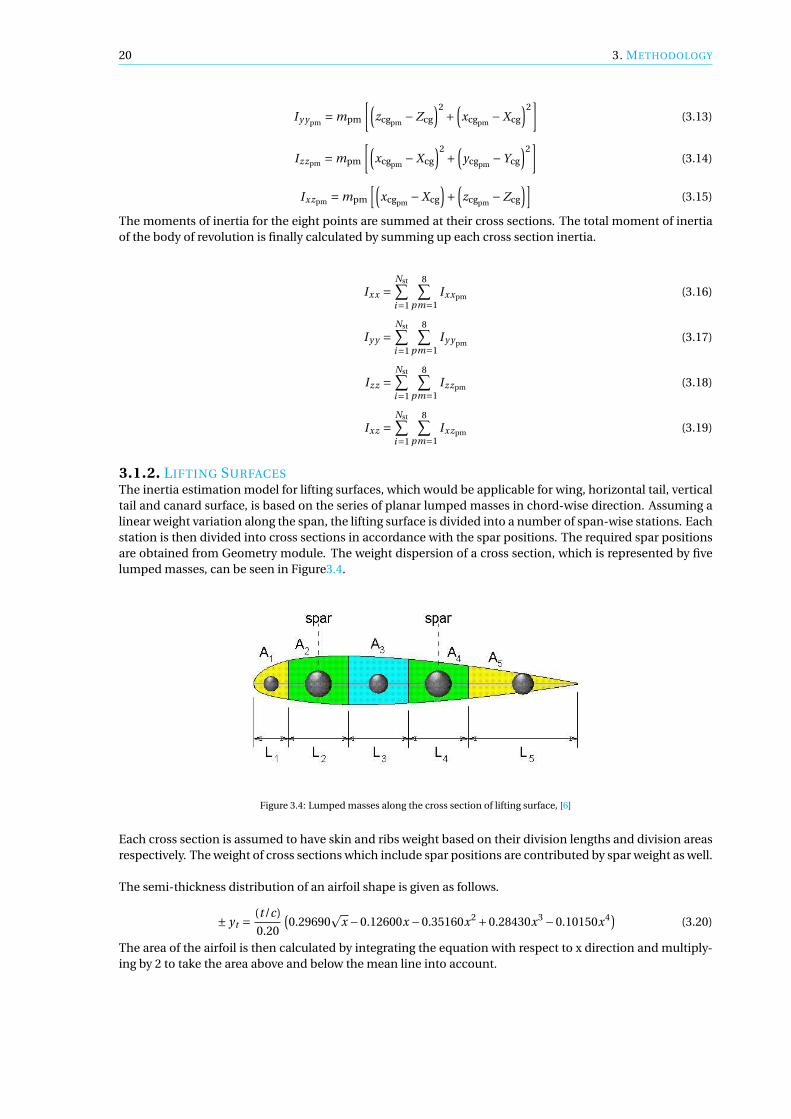
3.1.2. LIFTING SURFACESThe inertia estimation model for lifting surfaces, which would be applicable for wing, horizontal tail, verticaltail and canard surface, is based on the series of planar lumped masses in chord-wise direction. Assuming alinear weight variation along the span, the lifting surface is divided into a number of span-wise stations. Eachstation is then divided into cross sections in accordance with the spar positions. The required spar positionsare obtained from Geometry module. The weight dispersion of a cross section, which is represented by fivelumped masses, can be seen in Figure3.4.
Figure 3.4: Lumped masses along the cross section of lifting surface, [6]
Each cross section is assumed to have skin and ribs weight based on their division lengths and division areasrespectively. The weight of cross sections which include spar positions are contributed by spar weight as well.
The semi-thickness distribution of an airfoil shape is given as follows.
± yt = (t/c)
0.20
(0.29690
px −0.12600x −0.35160x2 +0.28430x3 −0.10150x4) (3.20)
The area of the airfoil is then calculated by integrating the equation with respect to x direction and multiply-ing by 2 to take the area above and below the mean line into account.
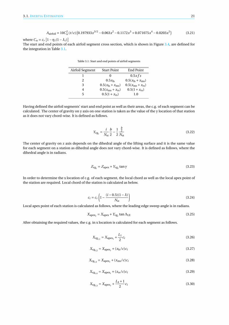
3.1. INERTIA ESTIMATION 21
Aairfoil = 10C 2n (t/c)
(0.197933x3/2 −0.063x2 −0.1172x3 +0.071075x4 −0.0203x5) (3.21)
where Cn = cr[1−ηi (1−λi )
]The start and end points of each airfoil segment cross section, which is shown in Figure 3.4, are defined forthe integration in Table 3.1.
Table 3.1: Start and end points of airfoil segments
Airfoil Segment Start Point End Point
1 0 0.5x f s2 0.5xfs 0.5(xfs +xms)3 0.5(xfs +xms) 0.5(xms +xrs)4 0.5(xms +xrs) 0.5(1+xrs)5 0.5(1+xrs) 1.0
Having defined the airfoil segments’ start and end point as well as their areas, the c.g. of each segment can becalculated. The center of gravity on y axis on one station is taken as the value of the y location of that stationas it does not vary chord-wise. It is defined as follows.
Ycgi= i
Nst
b
2− 1
2
b2
Nst(3.22)
The center of gravity on z axis depends on the dihedral angle of the lifting surface and it is the same valuefor each segment on a station as dihedral angle does not vary chord-wise. It is defined as follows, where thedihedral angle is in radians.
Zcgi= Zapex +Ycgi
tanγ (3.23)
In order to determine the x location of c.g. of each segment, the local chord as well as the local apex point ofthe station are required. Local chord of the station is calculated as below.
ci = cr
(1− (i −0.5)(1−λ)
Nst
)(3.24)
Local apex point of each station is calculated as follows, where the leading edge sweep angle is in radians.
Xapexi= Xapex +Ycgi
tanΛLE (3.25)
After obtaining the required values, the c.g. in x location is calculated for each segment as follows.
Xcgi ,1= Xapexi
+ L1
2ci (3.26)
Xcgi ,2= Xapexi
+ (xfs/c)ci (3.27)
Xcgi ,3= Xapexi
+ (xms/c)ci (3.28)
Xcgi ,4= Xapexi
+ (xrs/c)ci (3.29)
Xcgi ,5= Xapexi
+ L4 +1
2ci (3.30)

22 3. METHODOLOGY
The lifting surface is finally represented by lumped masses distributed along both the chord and span thatcan be seen in Figure 3.5.
Figure 3.5: Representation of the lifting surface with lumped masses, positioned wrt fuselage nose
In order to find a trade in weight distribution along stations, an intermediate calculation parameters is intro-duced as
par = B1 − A1 (3.31)
where A1 and B1 represents masses of first and second station respectively. They are found by the use ofderivative of the linearly varied mass along the span which is defined as
a =−m
cr (1−λ)∑ci
Nst
2
(3.32)
Using this parameter A1 and B1 are calculated as follows.
A1 = b2
4N 2st
a
2+ b
2NstC1 (3.33)
B1 = 3b2
2N 2st
a
4+ b
2NstC1 (3.34)
where the constant C1 is
C1 = 2
b
(m
2− b2
8a
)(3.35)
Hence, the intermediate calculation parameter is found by the difference of A1 and B1. Having calculatedthose parameters the chord-wise weight distribution along one station can be calculated. As mentioned,the chord-wise weight distribution is dependent on the area and length of each segment which are alreadycalculated. Besides those geometrical parameters, the fraction of skin, ribs and spar weights to the wholewing weight are required. However, the EMWET module in Initiator does not provide those required weight

3.1. INERTIA ESTIMATION 23
components separately. Because of this lack, the skin and spar weight contributions are calculated by theuse of thickness outputs of EMWET as well as already known wing geometry parameters such as chord andspan lengths. Both skin and spar geometries are assumed to be rectangular frustum which can be seen inFigure3.6.
Figure 3.6: Rectangular frustum
The volume of a truncated rectangular frustum is given as
V = h
6
[LH + (L+L′)(H +H ′)+L′H ′] (3.36)
where h, L, and H represent height, length and height respectively and all of which are shown in the Figure3.6. In the equation, the characters with prime represent the same but for the ending surface of the geometry.In other words, for a wing while L and H represent the length height of the root surface, L′ and H ′ representthe length and height of the tip surface. In the presence of a kink on the wing, the volume has to be calculatedfrom root to kink and kink to tip and summed up.
Airfoil non-dimensional coordinates (U,V) from trailing edge to leading edge and from there to trailing edgeare imported from Ai r f oi l object in Initiator for each section (root,kink,tip). Upper and lower V points areobtained for each U point, whose example can be seen in Figure 3.7. Obtained coordinates are scaled to thelocal chord length in order to get the real airfoil thickness at that section. This airfoil data is used in furthercalculations of weight contributions.

24 3. METHODOLOGY
Figure 3.7: Example of an airfoil coordinates
The calculation of spar weight fraction starts by defining parameters. The thickness of the spar at one sectionis defined as H in Figure 3.6 and the thickness of the spar at the next section as H ′. The height of the sparis represented by the L in Figure 3.6 while L′ represents the height at the following section. The distance be-tween two sections is defined by h.
To begin with, the U point on the chord which represents the spar position is found which is followed by ob-taining the corresponding upper and lower V data. The length of the spar in z direction is calculated by thedistance between gathered V data. The procedure is followed for each spar at each section which results inthe required L and L′ values for all. The thickness of the spars at each section is gathered as an output fromEMWET module. Hence, H and H ′ values are found as well. The remaining required value, h is calculatedfor each segment, i.e from root to kink and from kink to tip, by multiplying the span length with span-wisesection position differences. After obtaining the geometrical parameters, the volume of the spar is calculatedand multiplied by the density of the spar material.
The calculation of the skin weight fraction starts assuming the skin consists of panels in order to find the arclength in an easier approach. On the contrary to geometry definitions of spar calculations, L in Figure 3.6is taken as the thickness and H as the skin length. The assumed panel lengths are calculated by the use ofairfoil points U and V. Hence, the H and H ′ values of the upper and lower skin are found by the total panellength. L and L′ values, which represent the thicknesses at successive sections, are obtained from EMWET.The distance from one section to the other, which is represented by h in the Figure 3.6, is calculated by theuse of same logic that is used for the h in spar calculations. Hence, tThe volume of the upper and lower skinare calculated by the use of calculated geometrical parameters. The result is multiplied with the density ofthe skin material so that the weight contribution of the skin is achieved.
Ribs weight contribution to the wing is calculated by [16] as follows.
mrib = krρmaterialSw
(tr e f +
trw + ttw
2
)(3.37)
where kr = 0.5×10⁻³, tref = 1.0m, and trw and ttw represents the thicknesses of rib at root and tip sections.

3.1. INERTIA ESTIMATION 25
Having obtained all required parameters, chord-wise weight distribution is calculated as below.
Wi ,1 =[
L1Fskin +( Aairfoilsegment1i
Aairfoili
)Fribs
][A1 +par (i −1)
](3.38)
Wi ,2 =[
(L2 −L1)Fskin +( Aairfoilsegment2i
Aairfoili
)Fribs +Ffs
][A1 +par(i −1)
](3.39)
Wi ,3 =[
(L3 −L2)Fskin +( Aairfoilsegment3i
Aairfoili
)Fribs +Fms
][A1 +par(i −1)
](3.40)
Wi ,4 =[
(L4 −L3)Fskin +( Aairfoilsegment4i
Aairfoili
)Fribs +Frs
][A1 +par(i −1)
](3.41)
Wi ,5 =[
(1−L4)Fskin +( Aairfoilsegment5i
Aairfoili
)Fribs
][A1 +par(i −1)
](3.42)
After calculating weight and c.g. of each point mass, the moment of inertia at each station can be determinedas follows.
Ixxi , j = mi , j
[(ycgi
−Ycg)2 + (
zcgi−Zcg
)2]
(3.43)
Iy y i , j= mi , j
[(zcgi
−Zcg)2 +
(xcgi , j
−Xcg
)2]
(3.44)
Izzi , j = mi , j
[(xcgi , j
−Xcg
)2 + (ycgi
−Ycg)2
](3.45)
Ixzi , j = mi , j
[(xcgi , j
−Xcg
)+ (
zcgi−Zcg
)](3.46)
The moments of inertia of five point masses which represent five airfoil segments are summed at their station.The total moment of inertia of the lifting surface is finally calculated by summing up each station’s inertiavalue and multiplying by 2.
Ixx = 2Nst∑i=1
5∑j=1
Ixxi , j (3.47)
Iy y = 2Nst∑i=1
5∑j=1
Iy yi , j (3.48)
Izz = 2Nst∑i=1
5∑j=1
Izzi , j (3.49)
Ixz = 2Nst∑i=1
5∑j=1
Ixzi , j (3.50)
HORIZONTAL AND VERTICAL STABILIZER
Initiator does not use EMWET for the weight calculations of horizontal and vertical stabilizers which is whythe mentioned methodology of lifting surface inertia calculations cannot be used. The required separate skin,spar and ribs weights can not be calculated due to the lack of thicknesses of those components. Therefore,DATCOM [5] method is implemented in order to find the moment of inertia of lifting surfaces in the absenceof EMWET results.
In order to calculate the pitching and yawing moment of inertia of the horizontal and vertical surfaces respec-tively, DATCOM represents the lifting surface and the mass distribution with respect to this surface shape inFigure 3.8

26 3. METHODOLOGY
Figure 3.8: Surface shape and its corresponding mass distribution, [5]
Here, Ca , Cb , and Cc represent the smallest, intermediate and the largest value of the following parameters
crbt anΛLE
2 ct + bt anΛLE2
The slopes of mass distribution graph, y1, y2, and y3 from 0 to Ca , Ca to Cb and Cb to Cc respectively, aredefined as below.
y1 = ρ
Cax (3.51)
y2 = ρ (3.52)
y3 =− ρ
Cc −Cbx + ρCc
Cc −Cb(3.53)
where ρ is the weight to chord ratio of the surface and is calculated as follows.
ρ = W
0.5(−Ca +Cb +Cc )(3.54)
The inertia is derived by assumed mass distribution is written as follows.
I = ρ
12
(−C 3a +C 3
b +C 2c Cb +CcC 2
b +C 3c
)(3.55)
Hence, moment of inertia on its own centroid is calculated as follows, where the o in subscripts represent thecentroidal inertia.
Io = Ko
[I − (
∑mx)2∑
m
](3.56)
where Ko is an empirical constant and is given as 0.771 for any horizontal and vertical stabilizer [5].
Horizontal Stabilizer Pitching
The centroidal pitching moment of inertia of the horizontal stabilizer is calculated by solving Equation 3.56with substitution of horizontal stabilizer parameters.
Horizontal Stabilizer Rolling
The centroidal rolling moment of inertia is given by the following equation.

3.1. INERTIA ESTIMATION 27
Iox =W b2K4
24
(crht +3ctht
crht + ctht
)(3.57)
where the constant K4 is obtained from the Figure B.1 given in Appendix B.
The centroidal yawing moment of inertia is given as
Ioz = Ioy + Iox (3.58)
Vertical Stabilizer RollingThe centrodial rolling moment of inertia for the vertical stabilizer is given as
Iox =Wv b2
v K5
18
(1+ 2crv ctv
(crv + ctv )2
)(3.59)
where the constant K5 is obtained from the Figure B.2 given in Appendix B.
Vertical Stabilizer YawingIt is calculated by solving equation 3.56 with vertical stabilizer parameters.
Vertical Stabilizer PitchingThe centroidal pitching moment of inertia for the vertical stabilizer is the sum of rolling and yawing momentsof inertia.
Ioy = Iox + Ioz (3.60)
Having calculated the moment of inertia values about the centroidal axis of the bodies, the total moment ofinertia can be calculated. Following equations are solved for both horizontal and vertical surfaces by substi-tuting respective parameters.
Ixx = Iox +mstab
((ycgstab
−Ycg)2 + (
zcgstab−Zcg
)2)
(3.61)
Iy y = Ioy +mstab
((xcgstab
−Xcg)2 + (
zcgstab−Zcg
)2)
(3.62)
Izz = Ioz +mstab
((xcgstab
−Xcg)2 + (
ycgstab−Ycg
)2)
(3.63)
Ixz = mstab(xcgstab
−Xcg)(
zcgstab−Zcg
)(3.64)
3.1.3. POINT MASSESRemaining aircraft components are assumed to be point masses for simplicity. The inertia estimation of thepoint masses are calculated by following equations.
Ixx = mcomp
((ycgcomp
−Ycg
)2 +(zcgcomp
−Zcg
)2)
(3.65)
Iy y = mcomp
((xcgcomp
−Xcg
)2 +(zcgcomp
−Zcg
)2)
(3.66)
Izz = mcomp
((xcgcomp
−Xcg
)2 +(
ycgcomp−Ycg
)2)
(3.67)
Ixz = mcomp
(xcgcomp
−Xcg
)(zcgcomp
−Zcg
)(3.68)

28 3. METHODOLOGY
3.2. CONTROL AND STABILITY DERIVATIVES ESTIMATIONHandling qualities are significantly dependent on the stability and control properties of the aircraft [17].Those characteristics are essential to be determined to be able to analyze the aircraft dynamic behavior. Sta-bility and control characteristics of the aircraft are fundamentally contributed by the aerodynamics of theaircraft and its controls. The calculation method is directly based on [15].
3.2.1. STABILITY DERIVATIVESThe fundamental stability derivatives that are calculated for the purpose of the project
• Angle-of-attack stability derivativesCLα ,CDα ,Cmα
• Angle-of-sideslip stability derivatiesCyβ ,Clβ ,Cnβ
• Roll rate stability derivativesCyp ,Clp ,Cnp
• Pitch rate stability derivativesCLq ,CDq ,Cmq
• Yaw rate stability derivativesCyr ,Clr ,Cnr
ANGLE-OF-ATTACK STABILITY DERIVATIVES
Lift-due-to-angle-of-attack derivative, CLαLift-due-to-angle-of-attack derivative is contributed by wing-fuselage and horizontal stabilizers. Wing-fuselagecontribution, which is the wing-fuselage lift curve slope, is found by the multiplication of wing lift curve slopeand wing-fuselage interference factor which is dependent on equivalent fuselage diameter and wing span.The contribution of a horizontal stabilizer is calculated by the use of its lift curve slope, dynamic pressureratio to the one of the main wing, wetted area ratio, and downwash gradient or upwash gradient dependingon if it is the horizontal tail or the canard respectively.
Drag-due-to-angle-of-attack derivative, CDα
Drag-due-to-angle-of-attack derivative calculation is dependent on the calculated lift-due-to-angle-of-attackderivative, the aspect ratio of the main wing, Oswald factor and the lift coefficient at steady state level flight.
Pitching moment-due-to-angle-of-attack derivative, Cmα
Pitching moment-due-to-angle-of-attack derivative is calculated by lift-due-to-angle-of-attack derivative andairplane pitching moment variation with lift coefficient. The latter parameter is estimated by the differencebetween the location of the moment reference center, which is chosen to be the center of gravity of the mainwing in this project, in fractions of m.g.c. and the location of the aircraft aerodynamic center in fractions ofthe m.g.c.. The location of the aircraft aerodynamic center in fractions of the m.g.c. is computed by the useof wing-fuselage, horizontal tail, and canard aerodynamic center locations.
ANGLE-OF-SIDESLIP STABILITY DERIVATIVES
Sideforce-due-to-sideslip derivative, CyβThe sideforce-due-to-sideslip derivative is composed of three contributors which are the main wing, fuse-lage and vertical tail. The wing contribution is related to the dihedral angle. The fuselage contribution isdependent on the wing-fuselage interference factor and fuselage cross section area at the point where theflow ceases to be potential. Those parameters are calculated with respect to wing positioning in z-axis andequivalent fuselage diameter. Vertical tail contribution is computed by using vertical tail lift curve slope, ef-fective vertical tail and other vertical tail parameters such as the aspect ratio and sweep angle.
Rolling-moment-due-to-sideslip derivative, ClβRolling-moment-due-to-sideslip derivative is contributed by wing-fuselage combination, horizontal tail andvertical tail. Wing-fuselage contribution is a function of wing geometry parameters such as quarter-chord

3.2. CONTROL AND STABILITY DERIVATIVES ESTIMATION 29
sweep angle, semi-chord sweep angle, dihedral angle, and compressibility correction factors of those param-eters. The horizontal tail contribution is computed from the horizontal tail dihedral effect, and the ratio ofhorizontal tail area and span to the ones of main wing. The vertical tail contribution is found by using thesideforce-due-to-sideslip, and location of vertical tail with respect to the aircraft c.g. in x and z directions.
Yawing-moment-due-to-sideslip derivative, CnβYawing-moment-due-to-sideslip derivative is contributed by the wing, fuselage and vertical tail. However,the wing contribution is important only at high angles of attack which is why it is neglected in this project.The fuselage contribution is dependent on the ratio of fuselage side area and its maximum width to the onesof the wing.The ratio is multiplied with two empirical factors which are related to Reynold’s number and wing-fuselage interference separately. The vertical tail contribution is a function of the sideforce-due-to-sideslipderivative. Other required parameters in order to compute the contribution are related to the vertical tailpositioning with respect to aircraft aerodynamic center and the main wing span.
ROLL RATE DERIVATIVES
Side-force-due-to-roll-rate derivative, Cyp
The side-force-due-to-roll-rate derivative is primarily influenced by the vertical tail. It is the function of ver-tical tail contribution to sideforce-due-to-sideslip derivative, vertical tail positioning with respect to aircraftaerodynamic center, and main wing span.
Rolling-moment-due-to-roll-rate derivative, Clp
The rolling-moment-due-to-roll-rate derivative is contributed by the wing, horizontal tail and vertical tail.The horizontal tail contribution is computed by using the roll-damping derivative of the horizontal tail, andarea and span ratios of the horizontal tail to the wing. The vertical tail contribution is a function of verticalcontribution to side-force-due-to-sideslip, and the ratio of vertical tail position with respect to the aircraftaerodynamic center divided by the main wing span.
Yawing-moment-due-to-roll-rate derivative, Cnp
The yawing-moment-due-to-roll-rate derivative has two contributors which are the main wing and the ver-tical tail. The former contribution is calculated by considering the wing twist angle, flap deflection, and liftcurve slope. Vertical tail contribution depends on the vertical tail’s contribution to side-force-due-to-sideslip-angle derivative, main wing span, and the vertical tail positioning.
PITCH RATE DERIVATIVES
Lift-due-to-pitch-rate derivative, CLq
The lift-due-to-pitch-rate derivative is contributed by the wing, horizontal tail and the canard. The horizontaltail contribution is estimated by the lift curve slope of the canard, its dynamic pressure ratio the wing, andthe volume coefficient. Canard’s contribution, which is a negative contribution, is calculated with the sameprocedure with appropriate substitution of canard parameters for horizontal tail parameters.
Drag-due-to-pitch-rate derivative, CDq
The drag-due-to-pitch-rate derivative is assumed to be negligible.
Pitching-moment-due-to-pitch-rate derivative, Cmq
The pitching-moment-due-to-pitch-rate derivative is contributed by the wing, horizontal tail and the ca-nard. The horizontal tail and canard contributions are functions of their lift curve slope, volume coefficient,dynamic pressure ratio to the wing, their aerodynamic center positioning with respect to the aircraft centerof gravity.
YAW RATE DERIVATIVES
Side-force-due-to-yaw-rate derivative, Cyr
The side-force-due-to-yaw-rate derivative is primarily affected by the vertical tail. It is a function of verticaltail contribution to the side-force-due-to-sideslip-angle, vertical tail positioning and main wing span.
30 3. METHODOLOGY
Rolling-moment-due-to-roll-rate derivative, Clr
The rolling-moment-due-to-roll-rate derivative is influenced by the wing and vertical tail. The wing contri-bution is calculated by the use of wing lift coefficient, the slope of the rolling moment due to roll rate, theslope of the low-speed rolling moment due to yaw rate, wing twist and dihedral angles, flap deflection and itseffect on the rolling moment due to roll rate. The vertical tail contribution is determined by the vertical tailcontribution to side-force-due-to-sideslip-angle derivative, vertical tail positioning, and the main wing span.
Yawing-moment-due-to-yaw-rate derivative, Cnr
The yawing-moment-due-to-yaw-rate derivative is contributed by the main wing and the vertical tail. Thewing contribution is determined by wing lift coefficient, wing zero-lift drag coefficient, lift effect of the wingyaw damping derivative, and drag effect of the wing yaw damping derivative, where last two parameters arefunctions of wing taper ratio, quarter-chord sweep angle, and aspect ratio. The vertical tail contribution is af-fected by the vertical tail contribution to side-force-due-to-sideslip-angle derivative, vertical tail positioning,and main wing span.
3.2.2. CONTROL DERIVATIVESCalculated control derivatives are listed as follows.
• Aileron control derivativesCyδa
,Clδa,Cnδa
• Elevator control derivativesCLδe
,CDδe,Cmδe
• Rudder control derivativesCyδr
,Clδr,Cnδr
• Canardvator control derivativesCLδc
,CDδc,Cmδc
AILERON CONTROL DERIVATIVES
Side-force-due-to-aileron derivative, Cyδa
The side-force-due-to-aileron derivative is negligible for most conventional aileron arrangements which iswhy it is taken to be 0.
Rolling-moment-due-to-aileron derivative, Crδa
The rolling-moment-due-to-aileron derivative is dependent on inboard and outboard aileron locations, aileronrolling moment parameter, rolling effectiveness which is a function of aileron chord ratio to the wing, and thewing aspect ratio.
Yawing-moment-due-to-aileron derivative, Cnδa
The yawing-moment-due-to-aileron derivative is found by using the wing lift coefficient, rolling-moment-due-to-aileron derivative. Correction is applied for yawing moment due to aileron deflection, which is influ-enced by the wing taper ratio, aspect ratio and the lateral positioning of the aileron on the sing span.
RUDDER CONTROL DERIVATIVES
Side-force-due-to-rudder derivative, Cyδr
The side-force-due-to-rudder derivative is found from the vertical tail airfoil lift curve slope, effective verticaltail area, rudder-span factor, lift effect of the yaw damping derivative, and drag effect of the yaw dampingderivative.
Rolling-moment-due-to-rudder derivative, Crδr
The rolling-moment-due-to-rudder derivative is a function of the side-force-due-to-rudder derivative, mainwing span, and vertical tail positioning with respect to the aircraft center of gravity.

3.3. MATHEMATICAL MODEL FOR AIRCRAFT BEHAVIOR ESTIMATION 31
Yawing-moment-due-to-rudder derivative, Cnδr
The yawing-moment-due-to-rudder derivative is influenced by the same parameters with the rolling-moment-due-to-rudder derivative.
ELEVATOR CONTROL DERIVATIVES
Lift-due-to-elevator derivative, CLδe
The lift-due-to-elevator derivative is a function of the lift-due-to-stabilizer-incidence. The estimation is alsoaffected by the elevator span factor, chord ratio of the elevator to the horizontal tail, and the airfoil lift curveslope of the horizontal tail.
Drag-due-to-elevator derivative, CDδe
The drag-due-to-elevator derivative is computed in the same way as the lift, with the replacement of drag-due-to-stabilizer-incidence to the lift-due-to-stabilizer-incidence. Drag-due-to-stabilizer-incidence deriva-tive is influenced by the horizontal tail lift coefficient, aspect ratio, airfoil lift curve slope and dynamic pres-sure ratio to the wing.
Pitching-moment-due-to-elevator derivative, Cmδe
The pitching-moment-due-to-elevator derivative is also calculated by the same principle with the substitu-tion of pitching-moment-due-to-stabilizer-incidence to lift-due-to-stabilizer-incidence. The pitching-moment-due-to-stabilizer-incidence is affected by the horizontal tail airfoil lift curve slope, volume coefficient, dy-namic pressure ratio to the main wing.
CANARDVATOR CONTROL DERIVATIVES
Lift-due-to-canardvator derivative, CLδc
The lift-due-to-canardvator derivative is a function of the lift-due-to-canard-incidence derivative, which isinfluenced by the canard airfoil lift curve slope, and ratios of area and dynamic pressure ratio to the wing.The estimation is also affected by the canardvator span factor, chord ratio of the canardvator to the canard,and the airfoil lift curve slope of the canard.
Drag-due-to-elevator derivative, CDδc
The drag-due-to-elevator derivative is computed in the same way as the lift, with the replacement of drag-due-to-canard-incidence to the lift-due-to-canard-incidence. The drag-due-to-canard-incidence is a func-tion of the canard lift coefficient, airfoil lift curve slope, aspect ratio and dynamic pressure ratio to the wing.
Pitching-moment-due-to-canardvator derivative, Cmδc
The pitching-moment-due-to-canardvator derivative is also calculated by the same principle with the substi-tution of pitching-moment-due-to-canard-incidence to lift-due-to-canard-incidence. The pitching-moment-due-to-canard-incidence is determined by the canard airfoil lift curve slope, volume coefficient, and the dy-namic pressure ratio to the wing.
3.3. MATHEMATICAL MODEL FOR AIRCRAFT BEHAVIOR ESTIMATIONDetermination of the handling qualities of an aircraft requires aerodynamic forces and moments of the air-craft. They are calculated by using stability and control derivatives as follows.
X = (qS)
((CL −CDα )α−CDq
qc
2V−CDδe
δe
)(3.69)
Y = (qS)
(Cyββ+Cyp
pb
2V+Cyr
r b
2V+Cyδa
δa +Cyδrδr
)(3.70)
Z = (qS)
(−(CLα +CD )α−CLq
qc
2V−CLδe
δe
)(3.71)

32 3. METHODOLOGY
L = (qSb)
(Clββ+Clp
pb
2V+Clr
r b
2V+Clδa
δa +Clδrδr
)(3.72)
M = (qS)
(−(Cmαα+Cmq
qc
2V+Cmδe
δe
)(3.73)
N = (qSb)
(Cnββ+Cnp
pb
2V+Cnr
r b
2V+Cnδa
δa +Cnδrδr
)(3.74)

4VALIDATION
In order to ensure the credibility of implemented methods, a validation study is performed.
4.1. VALIDATION OF INERTIA ESTIMATION METHOD
4.1.1. ACCURACY OF THE IMPLEMENTED METHODIn order to be able to rely on the proposed inertia estimation method, validation of the programming is of im-portance. A validation on the accuracy of implemented method is performed with an example aircraft. Thereference aircraft is chosen to be Fokker 100 due to its available real data. Fokker 100 can be seen in Figure 4.1.
Figure 4.1: Reference aircraft Fokker 100
The comparison of the obtained values and real data are shown in Table 4.1.
Table 4.1: Comparison of moment of inertia values for Fokker100
Inertia (kg m2) Real Data Obtained Value Error Percentage
Ixx 252960 248000 1.96Iy y 1668670 1792600 7.43Izz 1846990 1958000 6.01Ixz 87200 74300 14.79
33

34 4. VALIDATION
The comparison of calculated values to real data shows that the error is less than 8 percent for the momentsof inertia. The highest error percentage occurs in Ixz product of inertia with 15 percent. Sensitivity analysisis conducted in order to see if those error percentages are acceptable in the estimation of handling qualities.Both longitudinal and lateral/directional handling qualities are examined using the real value and estimatedvalue of the inertia.
The comparison of phugoid damping ratio is shown in Table 4.2.
Table 4.2: Comparison of phugoid damping ratio values
Fokker 100 Data ζp Corresponding Level
Real data 0.0202 Level 2Estimated Ixx 0.0202 Level 2Estimated Iy y 0.0178 Level 2Estimated Izz 0.0202 Level 2Estimated Ixz 0.0202 Level 2
It is clearly seen that the phugoid damping ratio is only affected by the pitching moment of inertia Iy y , whichis an expected result as it is the only moment of inertia that influences longitudinal behavior of the aircraft.The difference of phugoid damping ratio is found to be 11 percent which in fact does not lead to any changein the level of handling quality.
Following the phugoid mode, the longitudinal behavior is examined by comparison of short period un-damped natural frequency values of each case whose result is shown in Figure 4.2.
Figure 4.2: Comparison of short period undamped natural frequency values
In Figure 4.2, it is seen that results of short period frequency requirement are matching for real data, real datausing estimated Ixx , real data using estimated Izz , and real data using estimated Ixz , while the result of realdata using estimated Iy y has a slight difference. This difference can be seen more clearly in Figure 4.3, and

4.1. VALIDATION OF INERTIA ESTIMATION METHOD 35
can evidently be said that it is negligible.
Figure 4.3: Comparison of short period undamped natural frequency values with different pitching moment of inertia
Obtained short period damping ratios for each study case and corresponding quality level are shown in Table4.3.
Table 4.3: Short period damping ratio results
Fokker 100 Data ζsp Corresponding Level
Real data 0.6516 Level 1Estimated Ixx 0.6516 Level 1Estimated Iy y 0.6594 Level 1Estimated Izz 0.6516 Level 1Estimated Ixz 0.6516 Level 1
Similar to phugoid damping ratio results, only difference in short period damping ratios appears in the datawith estimated Iy y .
CAP and short period damping ratio values each case are shown in Figure4.4.

36 4. VALIDATION
Figure 4.4: Comparison of CAP and short period damping ratio values
CAP and short period damping ratio requirements are precisely matching for each case except the real datausing estimated Iy y . The slight distinction can be seen in Figure 4.5.
Figure 4.5: Comparison of CAP and short period damping ratio values
The error percents in longitudinal handling quality requirements are found to be less than 12% which conse-

4.1. VALIDATION OF INERTIA ESTIMATION METHOD 37
quently does not influence the level. Hence, it can be concluded that the 7.43% error in pitching moment ofinertia Iy y is an acceptable value regarding the changes in longitudinal behavior of the aircraft.
Secondly, the lateral/directional handling quality requirements are examined in terms of their sensitivity tochanges in moment of inertia results.
Dutch roll undamped natural frequency and damping ratio results are shown in Table 4.4 .
Table 4.4: Comparison of Dutch roll undamped natural frequency and damping ratio
Fokker 100 Data ζd ωnd ζdωnd
Real data 0.8009 0.3622 0.2901Estimated Ixx 0.8013 0.3621 0.2902Estimated Iy y 0.8009 0.3622 0.2901Estimated Izz 0.7957 0.3547 0.2822Estimated Ixz 0.8010 0.3622 0.2901
Due to the fact that lateral/directional modes are only influenced by lateral/directional moments of inertia,the Dutch roll natural frequency and damping ratio results with estimated Iy y are precisely same with theones that are calculated using the real data. The Dutch roll natural frequency is inversely proportional tosquare root of yawing moment of inertia Izz . Therefore, the error percentage in the estimated value of Izz
is directly observed in the result of ωnd . Likewise, Dutch roll damping ratio is primarily influenced by Izz ,where only 0.65% error occurs due to a 6.01% error in the estimation of moment of inertia. Furthermore, theproduct of inertia Ixz , which has the highest error percentage compared to its real value, has almost negligibleeffect on Dutch roll.
The calculated spiral mode time constant values and their corresponding quality levels are presented in Ta-ble4.5.
Table 4.5: Comparison of minimum time to double the amplitude in spiral mode
Fokker 100 Data Min T2s (sec)
Real data -3.4768Estimated Ixx -3.4755Estimated Iy y -3.4768Estimated Izz -3.5351Estimated Ixz -3.4765
In Table reftable:F100spiralsensitivity it seen that the spiral time constant results are found to be negativeeven for the real data. Therefore the calculation process is checked in FMT in order to ensure the reliability.Same result is acquired by using the empirical spiral mode time constant equation given in Ref [? ]. Hence itcan be concluded that calculation process is reliable. However this shows that Fokker 100 is not satisfactoryto meet the spiral mode criteria.
Comparison of roll mode time constants are shown in Table 4.6.
Table 4.6: Comparison of roll mode time constant
Fokker 100 Data Tr (sec) Corresponding Level
Real data 0.2688 Level 1Estimated Ixx 0.2636 Level 1Estimated Iy y 0.2688 Level 1Estimated Izz 0.2687 Level 1Estimated Ixz 0.2688 Level 1

38 4. VALIDATION
The roll mode time constant is influenced directly by the rolling moment of inertia Ixx and slightly by theyawing moment of inertia Izz . An insignificant distinction on roll mode time constant is seen between thereal data and the real data using estimated Izz , which does not require a high concern. However, the influenceof the 1.9% lower estimation of Ixx is directly observed in Table 4.6, which shows that roll mode time constantis highly sensitive to the changes in Ixx . Owing to a good approximation of rolling moment of inertia, thedifference on results is acceptable.
4.1.2. COMPUTATION TIMEAs it is stated in the goal of the project, the estimation is required to be rapid. The computational time ofmoment of inertia estimation is found to be approximately 12 seconds, which is a satisfactory value.
4.2. VALIDATION OF CONTROL AND STABILITY DERIVATIVES ESTIMATION METHOD
4.2.1. ACCURACY OF THE IMPLEMENTED METHODIn order to be able to rely on the implementation of control and stability derivatives estimation method,validation of the programming is of importance. A validation on the accuracy of implemented method is per-formed with an example aircraft, which is chosen to be Boeing 747 due to its available data in Ref [18]. Boeing747-100 can be seen in Figure 4.6.
Figure 4.6: Reference aircraft Boeing 747-100
The comparison of longitudinal stability derivatives is shown in Table 4.7 with error percentages.
Table 4.7: Comparison of longitudinal stability derivatives of Boeing 747-100
Derivative (1/rad) Real Data Obtained Value Error Percentage
CLα 5.70 4.07 28.5CDα 0.66 0.57 13.66Cmα -1.26 -1.17 6.82CLq 5.4 4.69 13.15CDq NA 0 NACmq -20.80 -15.09 27.45
Among the obtained results CLα and Cmq have the highest error percentages. The former derivative is oneof the paramount parameters in longitudinal behavior, which means an error like this may result in big dif-

4.2. VALIDATION OF CONTROL AND STABILITY DERIVATIVES ESTIMATION METHOD 39
ferences. Unexpected behaviors in study cases may be explained due to a possible error in CLα calculations.Due to the lack data, a sensitivity analysis cannot be performed on this.The comparison of lateral stability derivatives is shown in Table 4.8 with error percentages.
Table 4.8: Comparison of lateral/directional stability derivatives of Boeing 747-100
Derivative (1/rad) Real Data Obtained Value Error Percentage
Cyβ -0.96 -0.68 29.16Clβ -0.22 -0.256 15.7Cnβ 0.15 0.139 7.53Cyp NA -0.1136 NAClp -0.45 -0.335 25.55Cnp -0.121 -0.186 53.72Cyr NA 0.593 NAClr 0.101 0.099 1.98Cnr -0.30 -0.32 6.67
Considering lateral/directional stability derivatives the highest error percentages are seen in derivatives dueto roll rate. Therefore, this should be taken into account in case of abnormal lateral/directional handlingquality results. Moreover, the side-force-due-to-sideslip-angle Cyβ has a high error compared to real value.However this can be acceptable since Cyβ has often negligible effect on the aircraft dynamics [19].
4.2.2. COMPUTATION TIMESimilar to inertia estimation module, the module for control and stability estimations is required to be rapid.The computational time of this estimation module is found to be approximately 3 seconds, which is a highlysatisfactory result.

5CASE STUDIES
In this chapter results of implemented methods are presented as well as their influence on handling qualityassessment.
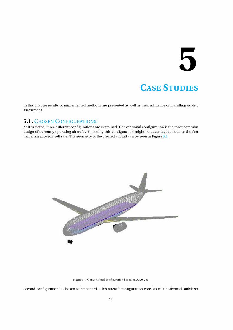
5.1. CHOSEN CONFIGURATIONSAs it is stated, three different configurations are examined. Conventional configuration is the most commondesign of currently operating aircrafts. Choosing this configuration might be advantageous due to the factthat it has proved itself safe. The geometry of the created aircraft can be seen in Figure 5.1.
Figure 5.1: Conventional configuration based on A320-200
Second configuration is chosen to be canard. This aircraft configuration consists of a horizontal stabilizer
41

42 5. CASE STUDIES
which is located in front of the main wing unlike the conventional configuration. The interest on the canardconfiguration aircraft dates back to the first days of aviation, which was Wright Brothers’ first flight attemptwith a heavier-than-air vehicle. [20] Following this, use of the canard has been experimented occasionallythroughout the history. Among the advantages and drawbacks of a canard configuration, the main differ-ence between such a configuration and the conventional tail airplane is the destabilizing pitching momentgeneration [20]. The aircraft model with a canard as a horizontal stabilizer is created based on a A320-200conventional aircraft, which can be seen in Figure5.2.
Figure 5.2: Canard configuration based on A320-200 conventional aircraft
Third study case is chosen to be three surface aircraft. A three surface configuration consists of main wing,canard and horizontal wing. The main purpose of this design is to locate the c.g. such that all surfaces cancontribute to the total lift. This leads to a reduction in induced drag but an increase in interference drag [20].There are few flying examples of this configuration, one of which is Piaggio P-180 Avanti. The aircraft modelhaving both a horizontal tail and a canard is created based on a A320-200 conventional aircraft, which can beseen in Figure5.3.

5.2. INERTIA ESTIMATION RESULTS 43
Figure 5.3: TSA configuration based on A320-200 conventional aircraft
Geometric parameters of components having high contributions to mass are presented in Appendix A foreach configuration.
5.2. INERTIA ESTIMATION RESULTSEstimated moment of inertia values for each configuration is presented in Table 5.1. The aircrafts have 37021kg, 32025 kg, and 36152 kg empty operating masses. Tsa has the highest values of inertia which means, theconfiguration would have a higher resistance to angular acceleration about any axis of rotation. The oppositeholds true for the canard configuration except about the pitching axis, where conventional configurationwould have a lower resistance.
Table 5.1: Estimated inertia of the conventional configuration
Inertia (kg m2) Conventional Canard TSA
Ixx 1062400 703300 1136100Iy y 3092400 3163400 3301300Izz 4015300 3778000 4257800Ixz 104470 36512 179390
Rolling moment of inertia Ixx is influenced by the mass distribution along y and z axes. Average fuselageheight and width of configurations are similar which leads to insignificant contribution to the differences ofIxx values. Therefore, the influence of mass distribution along z axis is dominated primarily by the tail. Eventhough the position of vertical tail at each configuration is almost the same, geometrical parameters andmasses are different which results in higher contribution in conventional configuration and followed by tsaand canard successively. Horizontal tail positioning has an important influence with respect to the significant
44 5. CASE STUDIES
difference in positioning between conventional and tsa. T-tail of tsa leads to significantly higher contributionthan the conventional tail configuration. When the mass distribution along the y axis is considered, distinc-tions occur primarily due to horizontal lifting surfaces and positioning of engines on them. Canard config-uration has its’ engines positioned relatively closer to the fuselage center section which lowers the momentarm and hence the moment of inertia. Engines of conventional and tsa configurations have their engines po-sitioned almost in same locations while the former has a larger mass than the latter configuration. This resultsin higher contribution of engines to the rolling moment of inertia of conventional aircraft. Despite the factthat engine contribution is highest in conventional configuration, tsa has the highest Ixx owing to one morehorizontal lifting surface than other two configurations, which results in significantly higher mass distribu-tion along y axis and to t-tail configuration which results in significantly higher mass distribution along z axis.
The pitching moment of inertia Iy y is influenced by the mass distribution along x and z axes. The fuselage hasan important contribution to Iy y having a large mass distributed along the roll axis. Moreover, Iy y is highlyaffected by tails’ positioning and masses, due to comparably long distances in x axis with respect to aircraftcenter of gravity. Likewise its effect on rolling moment of inertia, vertical positioning of the horizontal tailaffects the pitching moment of inertia. Results show that tsa has the highest Iy y which is followed by canardand conventional aircraft with 2% and 6% differences successively.
The yawing moment of inertia Izz is a function of the mass distribution along x and y axes. The reason behindIzz being the highest moment of inertia in each configuration, is the imposed effect of large mass distributionalong x axis due to highest mass contributor fuselage and comparably large mass distribution along y axis dueto second highest mass contributor main wing.
A significant difference between inertia values is seen in Ixz parameter. Canard configuration has a noticeablysmaller product of inertia compared to other two configurations. As the mathematical definition suggests,this inertial property is affected by the distance between aircraft c.g. and the position of the component onx and z axes. The primary reason of such a distinction is the approximately 20% lower fuselage mass of thecanard configuration.
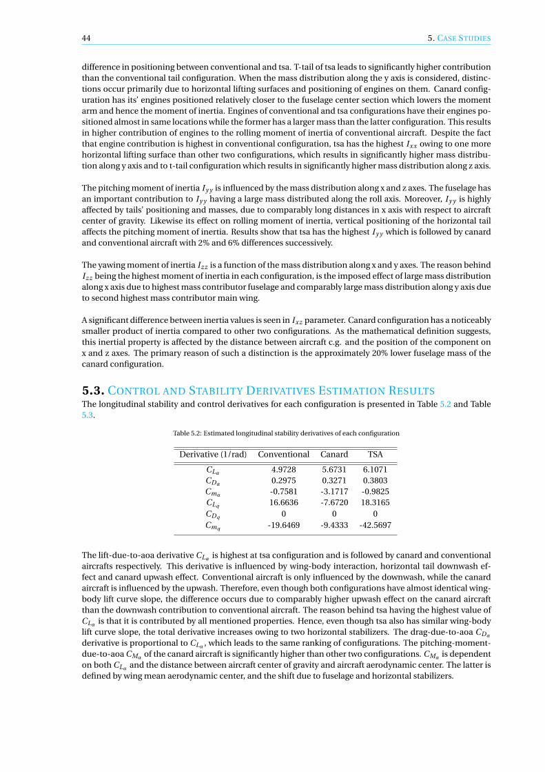
5.3. CONTROL AND STABILITY DERIVATIVES ESTIMATION RESULTSThe longitudinal stability and control derivatives for each configuration is presented in Table 5.2 and Table5.3.
Table 5.2: Estimated longitudinal stability derivatives of each configuration
Derivative (1/rad) Conventional Canard TSA
CLα 4.9728 5.6731 6.1071CDα 0.2975 0.3271 0.3803Cmα -0.7581 -3.1717 -0.9825CLq 16.6636 -7.6720 18.3165CDq 0 0 0Cmq -19.6469 -9.4333 -42.5697
The lift-due-to-aoa derivative CLα is highest at tsa configuration and is followed by canard and conventionalaircrafts respectively. This derivative is influenced by wing-body interaction, horizontal tail downwash ef-fect and canard upwash effect. Conventional aircraft is only influenced by the downwash, while the canardaircraft is influenced by the upwash. Therefore, even though both configurations have almost identical wing-body lift curve slope, the difference occurs due to comparably higher upwash effect on the canard aircraftthan the downwash contribution to conventional aircraft. The reason behind tsa having the highest value ofCLα is that it is contributed by all mentioned properties. Hence, even though tsa also has similar wing-bodylift curve slope, the total derivative increases owing to two horizontal stabilizers. The drag-due-to-aoa CDα
derivative is proportional to CLα , which leads to the same ranking of configurations. The pitching-moment-due-to-aoa CMα of the canard aircraft is significantly higher than other two configurations. CMα is dependenton both CLα and the distance between aircraft center of gravity and aircraft aerodynamic center. The latter isdefined by wing mean aerodynamic center, and the shift due to fuselage and horizontal stabilizers.

5.3. CONTROL AND STABILITY DERIVATIVES ESTIMATION RESULTS 45
Among longitudinal derivatives, the most noticeable difference is seen in the lift-due-to-pitch-rate derivative,CLq due to different sign of canard configuration. This derivative is contributed by horizontal lifting surfaces,and it highly depends on those surfaces’ aerodynamic center positions with respect to aircraft center of grav-ity. Wing contribution is computed by using the distance between aircraft c.g. and wing mean aerodynamiccenter in x-direction. For canard configuration the wing mean aerodynamic center is in front of the aircraftc.g. which yields this distance negative and consequently leads to a negative lift derivative contribution. Thepitching-moment-due-to-pitch-rate derivative Cmq is too high for tsa which is due to high contributions ofboth wing and the horizontal tail. Due to high distances between those surfaces’ aerodynamic center and theaircraft center of gravity, the derivative results in such a large value.
Table 5.3: Estimated longitudinal stability and control derivatives of the conventional configuration
Derivative (1/rad) Conventional Canard TSA
CLδe0.2297 - 2.6055
CDδe0.9720 - 0.8381
Cmδe-0.7660 - -0.7625
CLδc- 0.2541 0.2639
CDδc- 1.0914 1.1334
Cmδc- 0.4892 0.6435
The pitching control is provided by the elevator or/and canardvator. In Table 5.3, it is clearly seen that hori-zontal tail and canard affects the pitching moment in opposite ways, where canardvator has a destabilizingeffect on pitching moment while the horizontal tail provides stabilizing effect.
The lateral/directional stability and control derivatives for each configuration is presented in Table 5.4 andTable 5.5.
Table 5.4: Estimated lateral/directional stability derivatives of each configuration
Derivative (1/rad) Conventional Canard TSA
Cyβ -0.4808 -0.5517 -0.6044Clβ -0.0994 -0.0735 -0.1128Cnβ -0.0302 -0.0535 -0.0784Cyp -0.0409 -0.0382 -0.0239Clp -0.2685 -0.2952 -2.0696Cnp -0.0703 -0.0609 -0.1098Cyr 0.2861 0.3104 0.2693Clr 0.0432 0.0253 0.0250Cnr -0.1728 -0.1806 -0.1507
Among the stability derivatives due to sideslip angle, the rolling-moment-due-to-sideslip-angle Clβ is relatedto roll stiffness of the aircraft, which provides the aircraft the tendency to fly with wings level. When the air-craft rolls to an angle, a weight component occurs in the y direction, which induces a sideslip velocity. Theproduct of this sideslip angle and Clβ tends to bring the wings level. This derivative is highly affected by themain wing dihedral angle, aspect ratio, and sweep angle as well as the wing-fuselage lift coefficient. Latterterm is significantly higher than for tsa than other two configurations which leads to the highest value of Clβ .
The yawing-moment-due-to-sideslip-angle derivative Cnβ represents the yaw stiffness of the aircraft, whichmeans a perturbation in β would produce a restoring yawing moment that tends to keep the velocity vectorin the plane of symmetry [19]. Therefore the aircraft should have a positive Cnβ in order to have a positive yawstiffness. The primary contributors to this derivative are the fuselage and vertical tail, where the former onehas a negative influence on the contrary to the positive contribution of vertical tail. In Table 5.4 it is seen thatnone of the configurations have positive yaw stiffness. These results show that yawing moment created by

46 5. CASE STUDIES
vertical tail of each configuration fails to overcome the fuselage drag due to large body side areas. This can beovercome by either designing the vertical tail larger or positioning it more rearward and higher with respectto aircraft center of gravity, in other words by making the vertical tail more effective.
The rolling-moment-due-to-roll-rate Clp , in other words damping-in-roll derivative, expresses the aircraft’sresistance to rolling, and should always be negative. Even though each configuration seems to achieve thedamping in roll, the tsa configuration has significantly higher value. This derivative is contributed by thewing and vertical tail. The reason of this notable value of tsa is found to be due to dihedral effect parameterof wing which is a function of wing position in z-direction and dihedral angle. Both conventional and canardconfigurations have low wings while tsa has higher wing which results in such a distinct result.
The yawing-moment-due-to-roll-rate Cnp is one of the cross derivatives, which means it causes coupling be-tween rolling and yawing motions. Both wing and vertical tail contributes to this derivative, where the verticaltail influence is comparably lower than the main wing. The tsa having the highest wing contribution is fol-lowed by the conventional and canard successively which is directly observed on the total derivatives.
In Table 5.4, one of the important derivatives is the rolling-moment-due-to-yaw-rate Clr which expresses across derivative. It is contributed by the wing and vertical tail, where the latter one is the primary contributor.This contribution is highly affected by the vertical tail aerodynamic center position with respect to the air-craft center of gravity. The difference between those points in both x and z axes is lowest for tsa configurationwhich results in the lowest primary contribution.
The yawing-moment-due-to-yaw-rate Cnr is expressed as damping-in-yaw derivative as well. It is alwaysnegative, which means a negative yawing moment will be generated due to the increase in profile and in-duced drag on left wing and the decrease on the right wing which is the result of yaw rate [19]. Cnr resultsof all configurations satisfy this condition. The derivative is contributed by the main wing and mainly bythe vertical tail. The highest yaw damping occurs in canard configuration while the lowest is in tsa. Similarto Cnr , this is due to tsa’s comparably smaller distance between its vertical tail aerodynamic center positionwith respect to the aircraft center of gravity, which is the fundamental property that determines the verticaltail contribution.
Table 5.5: Estimated lateral/directional control derivatives of each configuration
Derivative (1/rad) Conventional Canard TSA
Cyδa0 0 0
Clδa0.1127 0.4173 0.3766
Cnδa-0.0108 -0.0383 -0.0373
Cyδr0.8589 1.0937 1.2536
Clδr0.1010 0.1120 0.0993
Cnδr-0.4835 -0.5938 -0.6441
In most flight conditions it is desired to have a zero sideslip angle. This can be maintained with a positive yawstiffness, which does not hold for any of those configurations. In such situations, in an unsymmetrical thrustor in an unsymmetrical flow field due to turning flight, the sideslip angle is kept zero by using the controlmoments. This control is primarily by the rudder, and therefore the yawing-moment-due-to-rudder Cnδr
isan important parameter. Tsa having the highest Cnδr
has a higher rudder power compared to other configu-rations.
The rolling control is provided by the ailerons, while they also introduce a yawing moment. Therefore two pa-rameters are important in terms of the aileron effectiveness which are rolling-moment-due-to-aileron deriva-tive Clδa
and yawing-moment-due-to-aileron derivative Cnδa. Cnδa
expresses the aircraft’s tendency for ayawing motion to opposite side due to the higher drag induced on the side with downward aileron. Thisundesired situation is called adverse yaw and would be high in the canard aircraft, which would introducedifficulties in lateral control.

5.4. HANDLING QUALITIES COMPARISON 47
5.4. HANDLING QUALITIES COMPARISON
Having calculated the inertia matrix and control and stability derivatives, configurations are compared interms of several handling qualities criterion. Aircrafts are trimmed at same conditions which are presentedin Table 5.6.
Table 5.6: Trim conditions
Altitude 1000 mAirspeed 130 m/sFlight path angle 0 degHeading angle 0 degTurn rate 0 deg/sSideslip angle 0 degPitch attitude rate 0 deg/s
5.4.1. LONGITUDINAL HANDLING QUALITIES
Handling qualities related to longitudinal dynamics are examined considering two modes which are phugoidand short period.
PHUGOID MODE
As it has been mentioned, phugoid mode is an oscillatory mode which is lightly damped and has a low fre-quency. The resultant phugoid damping ratio of each configuration and its corresponding handling qualitylevel according to requirements in Table 2.1 is given in Table 5.7.
Table 5.7: Phugoid damping ratio of each configuration
Configuration ζph Corresponding Level
Conventional 0.0940 Level 1Canard 0.0317 Level 2TSA 0.0690 Level 1
As can be seen, only canard configuration cannot satisfy the handling quality in terms of phugoid dampingratio requirement.
SHORT PERIOD MODE
The obtained short period undamped natural frequency values of each study case are shown together in Fig-ure 5.4.
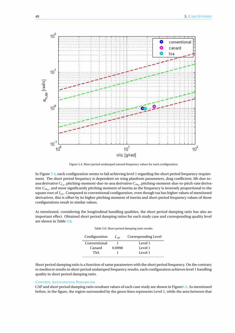
48 5. CASE STUDIES
Figure 5.4: Short period undamped natural frequency values for each configuration
In Figure 5.4, each configuration seems to fail achieving level 1 regarding the short period frequency require-ment. The short period frequency is dependent on wing planform parameters, drag coefficient, lift-due-to-aoa derivative CLα , pitching-moment-due-to-aoa derivative Cmα , pitching-moment-due-to-pitch-rate deriva-tive Cmq , and most significantly pitching moment of inertia as the frequency is inversely proportional to thesquare root of Iy y . Compared to conventional configuration, even though tsa has higher values of mentionedderivatives, this is offset by its higher pitching moment of inertia and short period frequency values of thoseconfigurations result in similar values.
As mentioned, considering the longitudinal handling qualities, the short period damping ratio has also animportant effect. Obtained short period damping ratios for each study case and corresponding quality levelare shown in Table 5.8.
Table 5.8: Short period damping ratio results
Configuration ζsp Corresponding Level
Conventional 1 Level 1Canard 0.6998 Level 1
TSA 1 Level 1
Short period damping ratio is a function of same parameters with the short period frequency. On the contraryto mediocre results in short period undamped frequency results, each configuration achieves level 1 handlingquality in short period damping ratio.
CONTROL ANTICIPATION PARAMETER
CAP and short period damping ratio resultant values of each case study are shown in Figure5.5. As mentionedbefore, in the figure, the region surrounded by the green lines represents Level 1, while the area between that

5.4. HANDLING QUALITIES COMPARISON 49
and blue lines represents Level 2. Level 3 is represented by the red lines.
Figure 5.5: CAP and short period damping ratio requirements
According to the Figure5.5 all configurations result in level 2 with respect to CAP and short period damp-ing ratio requirements, where conventional aircraft and tsa have really close results with conventional beingslightly closer to Level 1 zone. This is an expected outcome as CAP is proportional to the square of shortperiod frequency, where this parameter is found to be similar as well in Figure 5.4. Configurations need toachieve higher short period frequencies which would consequently lead to significantly higher CAP.
5.4.2. LATERAL/DIRECTIONAL HANDLING QUALITIESThree modes related to lateral/directional dynamics, namely Dutch roll, spiral and roll modes, are examinedfor each configuration.
DUTCH ROLL MODE
As mentioned, Dutch roll mode is assessed by its undamped natural frequency and damping ratio. Results ofeach configuration are shown in Table 5.9.
Table 5.9: Dutch roll undamped natural frequency and damping ratio results for each configuration
Configuration ζd ωnd ζdωnd
Conventional 0.1816 0.4576 0.0831Canard 0.1859 0.3785 0.0704TSA 0.2993 0.1985 0.0594

50 5. CASE STUDIES
According to Table 5.9, conventional aircraft is satisfactory in Dutch roll damping ratio and natural frequencyhaving level 1 handling quality. Canard and tsa meet the requirement of Dutch roll damping ratio howeverthey fail to have satisfactory results in natural frequency. Even the requirement of multiplication ends in level2 for the conventional aircraft, it can still be regarded as the most satisfactory configuration in terms of Dutchroll.
Dutch roll frequency is influenced directly by the square root of main wing area, span length, yawing-moment-due-to-sideslip-angle derivative Cnβ and inversely by the square root of yawing moment of inertia Izz . Thereason why conventional configuration satisfies the requirement is that it has noticeably larger main wingarea while having mediocre Cnβ and Izz . Other two configurations can be improved in terms of Dutch rollundamped natural frequency by obtaining an acceptable yaw stiffness which can be handled by a more ef-fective vertical tail.
SPIRAL MODE
The calculated spiral mode time constant values are presented in Table5.10.
Table 5.10: Results of minimum time to double the amplitude in spiral mode for each configuration
Configuration Min T2s (sec)
Conventional 2.3169Canard 2.48
TSA 3.0652
None of the configurations are satisfactory in spiral mode. Spiral mode time constant has dependency onyawing moment of inertia Izz , rolling-moment-due-sideslip-angle derivative Clβ , yawing-moment-due-to-sideslip-angle Cnβ , rolling-moment-due-to-roll-rate derivative Clp , yawing-moment-due-to-roll-rate deriva-tive Cnp , rolling-moment-due-to-yaw-rate derivative Clr , and yawing-moment-due-to-yaw-rate derivativeCnr . As it has been mentioned Clp and Cnp results may not be so reliable which may lead to such unusualtime constants.
ROLL MODE
Compared values are shown in Table 5.11.
Table 5.11: Roll mode time constant for each configuration
Configuration Tr (sec) Corresponding Level
Conventional 0.6264 Level 1Canard 0.4499 Level 1
TSA 0.1030 Level 1
The roll mode time constant varies inversely by the product of density and velocity. However, the difference oftime constant between configurations has no relation with that as they are trimmed at the same altitude andvelocity. Besides that relation, roll mode time constant is primarily influenced by rolling moment of inertiaIxx , where the higher is the rolling moment of inertia the more rapid is the response to the lateral input. It alsohas dependence on wing planform parameters, yawing moment of inertia Izz , rolling-moment-due-sideslip-angle derivative Clβ , yawing-moment-due-to-sideslip-angle Cnβ , rolling-moment-due-to-roll-rate derivativeClp , and yawing-moment-due-to-roll-rate derivative Cnp .
5.4.3. OVERVIEW OF LONGITUDINAL AND LATERAL/DIRECTIONAL MODESLongitudinal handling quality parameters include phugoid, short period mode and CAP requirements. Re-garding the phugoid mode, it is observed that only tsa is satisfactory to meet the phugoid damping ratiocriteria. It has been seen that configurations have similar results in short period which results in same han-dling quality levels. These parameters are primarily affected by the pitching moment which is influenced by

5.4. HANDLING QUALITIES COMPARISON 51
horizontal lifting surface sizing and position. Better positioning, i.e. longer distance in x-direction, wouldlead to better results. Hence, in terms of longitudinal behavior, tsa and conventional configurations havesimilar handling qualities and better performance than the canard configuration.
In order to have a clear sight on stability of those modes, eigenvalues of each mode of each configuration arepresented in Figure 5.6.
Figure 5.6: Eigenvalues of longitudinal modes
As it has been stated, longitudinal modes include two oscillatory modes which are phugoid and short period.Phugoid modes are recognized due to their light damping (i.e. smaller real part) and low oscillations (i.e.smaller imaginary part). Conversely short period modes are recognized by their high damping (i.e. larger realpart) and high high frequency (i.e. larger imaginary part). In Figure 5.6, it is seen that phugoid eigenvaluesfor each configuration are similar and stable. The conventional and tsa configurationa are found to have tworeal roots in short period mode, which is due to their damping ratio value of 1.
Lateral/directional handling qualities covers Dutch roll, spiral and roll modes. Dutch roll natural frequencyis directly proportional to yawing-moment-due-to-sideslip Cnβ and inversely proportional to yawing inertiaIzz . The reason why tsa fails to have a satisfactory handling quality with respect to Dutch roll frequency isthat it has a comparably higher Izz . As already mentioned, high Izz of tsa is because of the higher number ofpoint masses distributed along the y axis due to its three horizontal surfaces. Dutch roll damping is related toCnβ , Cyβ , Cnr derivatives which are highly contributed by the vertical tail geometry and position, and Izz . Allconfigurations satisfy the Dutch roll damping ratio requirement. Roll mode time constant, which is anotherassessment parameters of lateral/directional handling qualities, meets the requirement for each configura-tion.
In order to have a clear sight on stability of those modes, eigenvalues of each mode of each configuration are

52 5. CASE STUDIES
presented in Figure 5.7.
Figure 5.7: Eigenvalues of lateral/directional modes
As it has been mentioned, lateral/directional modes include one oscillatory and two real modes. In Figure5.7 roll mode eigenvalue of tsa seems to be too high which is not so reliable. Other two configuration hasreliable stable values. In order to see the differences of other modes, the figure is zoomed in Figure 5.8. Here,the Dutch roll eigenvalues for each configuration are found to be stable as they are on the negative side.Conventional and canard configurations have higher damping and higher oscillation compared to the tsa.Comparison of spiral eigenvalues show that all configurations have negative real value which actually wasnot expected as spiral has usually unstable (i.e positive) values.

5.4. HANDLING QUALITIES COMPARISON 53
Figure 5.8: Zoomed eigenvalues of lateral/directional modes


6CONCLUSION
The goal of this project has been defined as
Develop a rapid geometry-based inertia estimation method applicable for different aircraft configurationswhich would accelerate the estimation of handling qualities in a design environment
In order to reach this goal, the main question of the research has been determined as
How to estimate the inertial properties of conventional and unconventional configurations, as well as con-trol and stability derivatives, to assess handling qualities during the conceptual design phase?
The question was answered considering three parts. The first part focused on inertia estimation, which wasdetermined to be the main goal of the project. After conducting a literature research on existing inertia es-timation and weight estimation methods, based on the state-of-art, the aircraft was divided into three cate-gories namely bodies of revolution, lifting surfaces and point masses. Aircraft components were gathered inthose categories according to their shapes. Fuselage and nacelle bodies were categorized as bodies of revo-lution. Lifting surfaces included main wing, horizontal and vertical stabilizers as the name suggests. The restof the aircraft components were assumed to be point masses. Moments of inertia of components were calcu-lated according to their categorization. This classification has made the calculation process design sensitiveand rapid. Second part, which was related to control and stability derivatives estimation, was performed byimplementing an available empirical method directly to Initiator. Having calculated the required parameters,attention was given to handling qualities estimation. The outputs of implemented modules in Initiator wereused as input for the estimation of handling qualities in FMT.
The implemented method was used in different aircraft configurations. Both inertia and control and stabilityderivatives of each configuration were calculated in Initiator. They were used as inputs for Flight MechanicsToolbox to acquire handling qualities. Hence, the influence of configuration on its inertia and consequentlyon aircraft behavior has been able to examined in a rapid process. The confidence was gained on the accuracyof inertia estimation method by the validation. The error percentages found to be acceptable by conducting asensitivity analysis on handling quality assessment. A validation study is also performed on the implementedcontrol and stability derivatives estimation method. Calculated control and stability derivatives found tohave comparably higher error percentages. Therefore, the comparison of handling qualities with respect todifferent configurations can not be fully trusted due to low reliability of stability and control derivatives re-sults.
In terms of configuration comparison with respect to longitudinal handling quality assessment conventionalconfiguration and tsa configurations seem to have similar performances. According to lateral/directionalhandling qualities best performance was observed in conventional configuration. Hence, it can be concludedthat conventional aircraft would be the most satisfactory configurations regarding the handling quality as-sessment while the canard configuration would not be a preferable design.
55


7RECOMMENDATIONS
Based on the research performed and obtained results, several recommendations can be given for futureresearch and further improvements.
7.1. RECOMMENDATIONS RELATED TO INERTIA ESTIMATION METHOD
Inertia estimation method is created based on several calculation methods available in the literature. It isgiven high importance to have the method primarily geometry based. This aim was accomplished for theairframe structures fuselage, nacelle, and main wing. Even though the method implemented to estimate themain wing inertia would be suitable to use for other lifting surfaces, namely horizontal and vertical stabiliz-ers, this was not possible due to the lack of required structural input. As aforementioned in Section 3.1.2,in order to use the lifting surfaces inertia estimation method, weight fractions of spar, skin and ribs to totalcomponent weight are required. Since Inertia uses EMWET for the main wing weight calculations, those re-quired parameters were calculated by the use of wing planform parameters and EMWET thickness outputs.However the weight calculations of horizontal and vertical stabilizers are performed by Class 2.5 weight esti-mation methods. Therefore it is not possible to gather detailed structural information of those surfaces whichwould be subsequently used to calculate the weight fractions. It would be better to change from that methodof calculation into EMWET so that required structural parameters can be determined and the presented lift-ing surface inertia estimation method can be benefited. This way the empirical relations that are proposedby DATCOM can be omitted and a more physics based calculation of inertia can be performed. This wouldlead to a significant improvement on the total aircraft inertia estimation considering the sizes of those com-ponents.
Another future improvement related to estimation of inertia could be related to the systems and operationalitems. Weight and center of gravity information of those components are obtained from Class 2.5 weight es-timation module. According to the output, those components are considered to be point masses which arelocated at fuselage c.g. and their inertias are calculated in regard to that. Even though some changes weredone in positioning several items, such as repositioning APU more rearward or crew more forward, a layoutof the placement of each system along the whole aircraft can be created. This would be much more realisticas aircrafts do not have those items exactly at its fuselage c.g. but has them distributed along the body. More-over, even though items such as APU or instruments would make sense to be assumed as point masses, thisassumption is not as valid for hydraulics or residual fuel as former ones. Therefore, a layout can be assumedbased on existing aircraft knowledge which would be comparably more reliable. Hence, the more realistic thereplacement of systems and operational items are made, the more accurate the inertia estimation would be.
The validation of the method provided confidence in estimation of moment of inertia. However the errorpercentages can be decreased by considering mentioned recommendations for future work.
57

58 7. RECOMMENDATIONS
7.2. RECOMMENDATIONS RELATED TO CONTROL AND STABILITY DERIVATIVES
ESTIMATION METHODAs calculation of control and stability derivatives was not the main focus of this thesis, it has been performedby directly implementing the method proposed by [15]. Even though a validation study is performed a sensi-tivity analysis on handling quality assessment was not performed due to lack of further real data. Thereforethe influence of errors occurred in control and stability derivatives estimation on the handling qualities couldnot be checked. Finding real data of each required input would provide a handling quality comparison withrespect to changes in derivatives. Hence, the method can be improved according to outcome.
As it has been mentioned, the position and sizing of lifting surfaces are directly obtained from Geometrymodule, and do not depend on new design modules in Initiator due to the timing of this thesis. This yieldsmisleading results in especially stability derivatives as they are highly influenced by stabilizer parameters.Vertical tail position with respect to aircraft c.g. and its size is of importance in calculation of stability deriva-tives due to sideslip angle, roll and yaw rates which consequently affects lateral/directional handling qualitiesof the aircraft. An increase in vertical tail size or in distance with respect to aircraft c.g. that are obtained fromthe design modules could yield incomparably improved lateral stability. Likewise, a change in horizontal sta-bilizers’ either position or sizing would have a significant effect on longitudinal stability parameters since itis primarily influenced by that. Pitching moment, which is highly dependent on horizontal stabilizer param-eters, would have an improved result which would lead to improved longitudinal handling qualities.
Geometry of control surfaces has to be known in order to calculate the control derivatives. However Initiatordoes not have such a module that handles the stabilizer surface sizing. Therefore, a simple sizing of ailerons,rudder, elevator and canard control surface was performed with respect to the available aircraft knowledge.Since geometries of all case studies were created based on a A320-200, the sizing of the control surfaces wasalso done with respect to real sizing of that aircraft. Even though it would give proper results for similar air-crafts it can not be reliable for every configuration. Therefore control surface sizing should be done in a moregeneric way. Since moment of inertia and handling qualities of the aircraft would eventually have an effecton the sizing of these surfaces, the module to be created should have an iterative process concerning theseparameters and should be based on the feedback of those.
Estimation module of control and stability derivatives take angle of attack, angle of sideslip, pitch, roll andyaw rates derivatives leaving the derivatives due to velocity, angle of attack rate, and angle of sideslip rate. Thishas been done due to lack of time and due to their comparably negligible contributions on total aerodynamiccoefficients. In future studies, those derivatives can be added to estimation as well.

IIIMPLEMENTATION
59


8IMPLEMENTATION IN INITIATOR
For the purpose of this thesis, an in-house conceptual design tool Initiator is used for inertia and control andstability derivatives estimation. As it has been briefly covered in the tool description, the Initiator activitydiagram is presented in Figure 8.1.
Figure 8.1: Activity diagram of Initiator
The implementation of inertia estimation and control and stability derivative calculation methods in Initia-
61

62 8. IMPLEMENTATION IN INITIATOR
tor are explained by the help of activity diagrams in this chapter.
8.1. INERTIA ESTIMATION MODULE
Created inertia estimation module is dependent on the Aircraft Geometry and several results from Class 2.5Weight Estimation and EMWET modules. Based on the methodology that is presented in Chapter 3, the com-ponents’ inertias are calculated with different functions according to their shapes.
For the bodies of revolution, which contains fuselage and nacelle shaped components, the geometry data inX,Y,Z directions are gathered. The activity diagram of this function is shown in Figure 8.2.
Figure 8.2: Activity diagram of inertia estimation function of bodies of revolution
For the lifting surfaces the activity diagram is shown in Figure 8.3 where the process of subfunction for calcu-lation of the weight fractions are presented in Figure 8.4.

8.1. INERTIA ESTIMATION MODULE 63
Figure 8.3: Activity diagram of inertia estimation function of lifting surfaces

64 8. IMPLEMENTATION IN INITIATOR
Figure 8.4: Activity diagram of weight fractions calculation
For the rest of the aircraft components such as landing gear, systems and controls PointMassInertiaEstima-tion function is called. The activity diagram is shown in Figure 8.5.

8.2. CONTROL AND STABILITY DERIVATIVES ESTIMATION MODULE 65
Figure 8.5: Activity diagram of inertia estimation function of point masses
8.2. CONTROL AND STABILITY DERIVATIVES ESTIMATION MODULEThe control and stability derivatives estimation module has dependency on Class2.5 Weight Estimation andEMWET modules. The activity diagram is simply shown in Figure 8.6.
Figure 8.6: Activity diagram of control and stability derivatives estimation module
Activity diagrams for stability derivatives estimation are represented separately as follows.

66 8. IMPLEMENTATION IN INITIATOR
Stability derivatives due to angle of attack are shown in Figure8.7, Figure 8.8, and Figure8.9.
Figure 8.7: Activity diagram of lift-due-to-aoa derivative estimation

8.2. CONTROL AND STABILITY DERIVATIVES ESTIMATION MODULE 67
Figure 8.8: Activity diagram of drag-due-to-aoa derivative estimation
Figure 8.9: Activity diagram of pitching-moment-due-to-aoa derivative estimation

68 8. IMPLEMENTATION IN INITIATOR
Stability derivatives due to angle of sideslip are shown in Figure8.10, Figure8.11, and Figure8.12.
Figure 8.10: Activity diagram of side-force-due-to-sideslip derivative estimation

8.2. CONTROL AND STABILITY DERIVATIVES ESTIMATION MODULE 69
Figure 8.11: Activity diagram of rolling-moment-due-to-sideslip derivative estimation

70 8. IMPLEMENTATION IN INITIATOR
Figure 8.12: Activity diagram of yawing-moment-due-to-sideslip derivative estimation

8.2. CONTROL AND STABILITY DERIVATIVES ESTIMATION MODULE 71
Stability derivatives due to roll rate are shown in Figure8.13, Figure8.14, and Figure8.15.
Figure 8.13: Activity diagram of side-force-due-to-roll-rate derivative estimation
Figure 8.14: Activity diagram of rolling-moment-due-to-roll-rate derivative estimation

72 8. IMPLEMENTATION IN INITIATOR
Figure 8.15: Activity diagram of yawing-moment-due-to-roll-rate derivative estimation

8.2. CONTROL AND STABILITY DERIVATIVES ESTIMATION MODULE 73
Stability derivatives due to pitch rate are shown in Figure 8.16, Figure8.17, and Figure8.18.
Figure 8.16: Activity diagram of lift-due-to-pitch-rate derivative estimation
Figure 8.17: Activity diagram of drag-due-to-pitch-rate derivative estimation

74 8. IMPLEMENTATION IN INITIATOR
Figure 8.18: Activity diagram of pitching-moment-due-to-pitch-rate derivative estimation

8.2. CONTROL AND STABILITY DERIVATIVES ESTIMATION MODULE 75
Stability derivatives due to yaw rate are shown in Figure 8.19, Figure 8.20, and Figure 8.21.
Figure 8.19: Activity diagram of side-force-due-to-yaw-rate derivative estimation

76 8. IMPLEMENTATION IN INITIATOR
Figure 8.20: Activity diagram of rolling-moment-due-to-yaw-rate derivative estimation

8.2. CONTROL AND STABILITY DERIVATIVES ESTIMATION MODULE 77
Figure 8.21: Activity diagram of yawing-moment-due-to-yaw-rate derivative estimation

78 8. IMPLEMENTATION IN INITIATOR
Activity diagrams for control derivatives estimation method are shown in Figure8.22, Figure8.23, Figure8.24,and Figure8.25 for aileron, rudder, elevator and canardvator respectively.
Figure 8.22: Activity diagram of control derivatives due to aileron deflection estimation

8.2. CONTROL AND STABILITY DERIVATIVES ESTIMATION MODULE 79
Figure 8.23: Activity diagram of control derivatives due to rudder deflection estimation

80 8. IMPLEMENTATION IN INITIATOR
Figure 8.24: Activity diagram of control derivatives due to elevator deflection estimation

8.2. CONTROL AND STABILITY DERIVATIVES ESTIMATION MODULE 81
Figure 8.25: Activity diagram of control derivatives due to canardvator deflection estimation

9IMPLEMENTATION IN FLIGHT MECHANICS
TOOLBOX
In the scope of this thesis outputs of implemented methods in Initiator are used as inputs in another in-house tool Flight Mechanics Toolbox to obtain handling qualities. Hence in this chapter, the principle of FMTis covered. The adjustments that are made for the examined study cases are briefly explained.
9.1. FLIGHT MECHANICS TOOLBOX OVERVIEW
In order to observe the flight dynamics of an aircraft in the FMT, several steps have to be followed. To beginwith, a definition file has to be created for the aircraft that is to be examined. This file contains the assignedSimulink models which consider aerodynamics, control surfaces, propulsion system and AFCS with respectto the aircraft. Secondly, a data folder of the aircraft created by using the obtained results from Initiator.Creating the aircraft data file and the required inputs are explained briefly in Section 8.2. Last step beforesimulating the aircraft is to adjust the Module Library of the FMT which consists of several modules in re-lation with different disciplines. An adjustment according to the examined aircraft has to be made which isexplained in Section 8.3.
Having created the aircraft definition file, obtained the required inputs from already and newly implementedmodules in Initiator, and adapted the FMT modules considering the configuration of the aircraft, the flightdynamics analysis can be performed. The aircraft is trimmed with regard to desired conditions which is fol-lowed by gathering handling qualities results.
The procedure that is followed is shown in an activity diagram in Figure9.1.
9.2. CREATING AIRCRAFT DATA FILE
In order to observe the flight dynamics of an aircraft in the Flight Mechanics Toolbox, a data folder has tobe created which consists of aerodynamic, structure, engine and flight control surface data of the aircraft.Required aerodynamic data input are stability and control derivatives, which are calculated within the Con-trolStabilityDerivatives module in Initiator. The span, mean chord and the surface of the main wing are alsoinputs of aerodynamic data file and are gathered from Initiator. Structure data of aircraft includes the emptyweight and the moment of inertia both of which are obtained from Initiator. Required empty weight is ob-tained from the Class2.5WeightEstimation module whilst the latter input is the result of the implementedInertiaEstimation module. Engine data file requires the location of the engine(s) from the c.g., maximum andminimum thrust level and the thrust vector angle, which are obtained from Initiator as well. Last data filerelates to the flight control of the aircraft and hence control surfaces are defined here. Moreover, actuatorsdata and saturation limits of the control surfaces are assigned in this file.
83

84 9. IMPLEMENTATION IN FLIGHT MECHANICS TOOLBOX
Figure 9.1: Activity diagram of FMT
9.3. ADJUSTING THE MODULE LIBRARYBoth in the aeromodule and controlsurfacemodule aerodynamic forces and moments are calculated by theuse of stability and control derivatives respectively. The structure in Simulink is created according to theforces and moment equations in [15]. It should be noted that controlsurfacemodule has to be adapted ac-cording to the number of assigned control surfaces of the aircraft.

BIBLIOGRAPHY
[1] B. Chudoba, Stability and control of conventional and unconventional aircraft configurations: a genericapproach (BoD–Books on Demand, 2001).
[2] G. E. Cooper and R. P. Harper Jr, The use of pilot rating in the evaluation of aircraft handling qualities,Tech. Rep. (DTIC Document, 1969).
[3] J. Roskam, Airplane flight dynamics and automatic flight controls (DARcorporation, 1995).
[4] C. Lanham, Inertia Calculation Procedure for Preliminary Design, Tech. Rep. (DTIC Document, 1979).
[5] DATCOM 8.1 Aircraft Mass and Inertia, Tech. Rep. (USAF).
[6] J. P. Pegram and W. A. Anemaat, Preliminary estimation of airplane moments of inertia using CAD solidmodeling, Tech. Rep. (SAE Technical Paper, 2000).
[7] B. Stevens and F. Lewis, Aircraft Control and Simulation (Wiley, 2003).
[8] W. F. Phillips, Mechanics of flight (John Wiley & Sons, 2004).
[9] D. A. Caughey, Introduction to aircraft stability and control course notes for m&ae 5070, Sibley School ofMechanical & Aerospace Engineering, Cornell University, Ithaca, New York , 14853 (2011).
[10] R. Elmendorp, Synthesis of novel aircraft concepts for future air travel, Ph.D. thesis, TU Delft, Delft Uni-versity of Technology (2014).
[11] R. Schmidt, A semi-analytical weight estimation method for oval fuselages in novel aircraft configura-tions, Ph.D. thesis, TU Delft, Delft University of Technology (2013).
[12] T. Pfeiffer, B. Nagel, D. Bohnke, A. Rizzi, and M. Voskuijl, Implementation of a heterogeneous, variable-fidelity framework for flight mechanics analysis in preliminary aircraft design, in Proceedings of the 60Deutscher Luft-und Raumfahrtkongress, 27-29 September 2011, Bremen, Duitsland (DGLR, 2011).
[13] M. Voskuijl, J. de Klerk, and D. van Ginneken, Flight mechanics modeling of the prandtlplane for con-ceptual and preliminary design, in Variational Analysis and Aerospace Engineering: Mathematical Chal-lenges for Aerospace Design (Springer, 2012) pp. 435–462.
[14] E. Torenbeek, Synthesis of subsonic airplane design: an introduction to the preliminary design of subsonicgeneral aviation and transport aircraft, with emphasis on layout, aerodynamic design, propulsion andperformance (Springer Science & Business Media, 2013).
[15] J. Roskam, Airplane Design: Preliminary Calculation of Aerodynamic, Thrust and Power Characteris-tics. Determination of Stability, Control and Performance Characteristics: Far and Military Requirements.Airplane Cost Estimation, Design, Development, Manufacturing and Operating (Roskam aviation andengineering corporation, 1990).
[16] W. Liu and W. A. Anemaat, A refined method for wing weight estimation and a new method for wing centerof gravity estimation, in AIAA Aviation Technology Integration and Operation Conference, AIAA, Vol. 4371(2013).
[17] M. Cook, Flight Dynamics Principles: A Linear Systems Approach to Aircraft Stability and Control (Else-vier Science, 2012).
[18] R. Heffley and W. Jewell, Aircraft Handling Qualities Data, Tech. Rep. (NASA contractor report, 1972).
[19] B. Etkin, Dynamics of flight: stability and control (John Wiley & Sons Australia, Limited, 1982).
[20] S. Gudmundsson, General aviation aircraft design: applied methods and procedures (Butterworth-Heinemann, 2013).
85

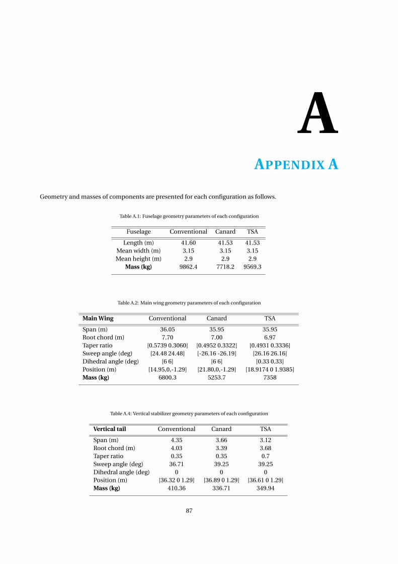
AAPPENDIX A
Geometry and masses of components are presented for each configuration as follows.
Table A.1: Fuselage geometry parameters of each configuration
Fuselage Conventional Canard TSA
Length (m) 41.60 41.53 41.53Mean width (m) 3.15 3.15 3.15Mean height (m) 2.9 2.9 2.9
Mass (kg) 9862.4 7718.2 9569.3
Table A.2: Main wing geometry parameters of each configuration
Main Wing Conventional Canard TSA
Span (m) 36.05 35.95 35.95Root chord (m) 7.70 7.00 6.97Taper ratio [0.5739 0.3060] [0.4952 0.3322] [0.4931 0.3336]Sweep angle (deg) [24.48 24.48] [-26.16 -26.19] [26.16 26.16]Dihedral angle (deg) [6 6] [6 6] [0.33 0.33]Position (m) [14.95,0,-1.29] [21.80,0,-1.29] [18.9174 0 1.9385]Mass (kg) 6800.3 5253.7 7358
Table A.4: Vertical stabilizer geometry parameters of each configuration
Vertical tail Conventional Canard TSA
Span (m) 4.35 3.66 3.12Root chord (m) 4.03 3.39 3.68Taper ratio 0.35 0.35 0.7Sweep angle (deg) 36.71 39.25 39.25Dihedral angle (deg) 0 0 0Position (m) [36.32 0 1.29] [36.89 0 1.29] [36.61 0 1.29]Mass (kg) 410.36 336.71 349.94
87

88 A. APPENDIX A
Table A.3: Horizontal lifting surface geometry
Horizontal Tail Conventional Canard TSA
Span (m) 9.17 - 7.69Root chord (m) 2.72 - 2.28Taper ratio 0.35 - 0.35Sweep angle (deg) 27.41 - 29.30Dihedral angle (deg) 6 - 0.33Position (m) [37.64 0 1.29] - [39.43 0 4.42]Mass 427.58 - 353.21
Canard
Span (m) - 10.73 10.90Root chord (m) - 2.96 3.01Taper ratio - 0.45 0.45Sweep angle (deg) - 23.55 23.55Dihedral angle (deg) - 0 -0.17Position (m) - [6.2291 0 1.6154] [4.1527 0 -1.6154]Mass (kg) - 534.52 524.71
Table A.5: Engine geometry parameters of each configuration
Engine Conventional Canard TSA
Length (m) 3.52 3.30 3.30Diameter (m) 1.93 1.70 1.75
Position [15.1952 6.3093 -2.1097] [29.0691 3.1746 0] [19.6303 6.2918 0.6117][15.1952 -6.3093 -2.1097] [29.0691 -3.1746 0] [19.6303 -6.2918 0.6117]
Mass (kg) 2656.4 2274.1 2274.1

BAPPENDIX B
89

90 B. APPENDIX B
Figure B.1: Horizontal stabilizer rolling inertia K factor, [5]

91
Figure B.2: Vertical stabilizer rolling inertia K factor, [5]


![Modelling Requirements to Assess the Resilience of The ...Inertia estimation using WAMS in GB network [27] Wind plant Inertia estimation [28] Frequency and power [29] Modelling Requirements](https://img.dokumen.tips/doc/110x75/5f41845fcdb69d1eee39dd8b/modelling-requirements-to-assess-the-resilience-of-the-inertia-estimation-using.jpg)