The development and evaluation of analytical methods for

i

The development and evaluation of analyticalmethods for the analysis of trace levels of moisture

in high purity gas samples

By

B.L. Hickman Mosdell

A Dissertation submitted in fulfillment of the requirements for the degree

Master of Science

In the Faculty of Sciences

at the University of the Witwatersrand, Johannesburg

Johannesburg, January 2015

ii

DECLARATION

I, BL Hickman Mosdell, hereby declare that the work on which this thesis is

based, has not, to m y knowledge, previously been submitted for a degree

at this or any other university. This work is my own and all reference

material that that has been used or quoted has been indicated and

acknowledged.

_________________

BL Hickman Mosdell

________________day of_______________20 ___in ________________

iii

ABSTRACT

Three methods, for the analyses of low levels of moisture in gas samples,

were developed and optimized. The analytical techniques included Fourier

Transform Infrared Spectroscopy (FTIR) and Pulsed Discharge Helium

Ionization/Gas Chromatography (PDHID/GC).

The methods included the direct analyses of moisture in gas samples

using FTIR as well as the analysis of acetylene (C2H2) by FTIR and

GC/PDHID. For the latter methods, the purpose was to convert the

moisture in a gas sample to C2H2 by hydrolization of the calcium carbide

(CaC2) with moisture to C2H2 and then analyze the resulting C2H2 content

by FTIR or GC/PDHID. The C2H2 result was then converted back to

moisture to obtain the moisture content of the sample.

The FTIR moisture method developed provided eleven different

wavenumbers for quantitation providing a wide analytical scope,

specifically in complex gas matrices, where there is often peak overlap

between matrix and moisture. A heated eight meter glass long path gas

cell and a mercury cadmium telluride (MCT) detector were utilized. The

FTIR method required much greater volumes of sample than the GC

method but allowed for direct analysis of moisture without prior conversion

to acetylene. Moisture permeation standards were used for calibration and

the LOD’s ranged from 0.5 to 1 ppm with quantification possible from 0.5

to 10ppm.

For the FTIR C2H2 method various concentration ranges were established

from 50 up to 2000 ppm. Three wavenumbers were evaluated for C2H2

and methane was introduced as an internal standard. The use of methane

as an internal standard provided better r2 values on the calibration data

than for the tests run without internal standard.

A gas chromatographic (GC), pulsed discharge helium ionization detector

(PDHID) method for the determination of moisture content in small

iv

quantities of gases, based on the conversion of the moisture to acetylene

(C2H2) prior to analysis, was developed. The method developed on the

GC/PDHID for C2H2, provided a quantitation range from 0.6 to 7.7 ppm.

Conversion of the moisture to acetylene was achieved by hydrolysing an

excess of calcium carbide (CaC2) in a closed reaction vessel with a

measured volume of a sample containing a known quantity of moisture.

The gaseous reaction mixture was transferred, using helium (He) carrier

gas, to a GC/PDHID, set up with “sample injection and heart cut to

detector” to prevent matrix disturbances on the PDHID, for analysis. The

acetylene concentration values thus obtained were converted back to

moisture values and percentage recoveries calculated. A similar

conversion process was applied on FTIR.

The conversion of moisture to C2H2 using CaC2 was tested and proven to

be viable. Quantification was not possible as the available sample holder

could not be adequately sealed to prevent air ingress. This led to higher

C2H2 values than expected. This process can be optimized by the design

and production of a sealed sample holder.

.

v

ACKNOWLEDGEMENTS

There were so many people supporting and encouraging me throughout

this project. I would firstly like to thank my wonderful, supportive and

patient husband, John Mosdell who spent many weekends alone while I

worked on this thesis.

I would like to thank Jacques Richer, my friend and colleague who gave

me so many great ideas and was ever there as a sounding board and

advisor.

I must thank Johan van der Westhuizen for his endless patience when it

came to building and modifying the systems, often more than once!

Thank you to my manager, Lenie Heystek, for believing in me and trying to

relieve the works pressure wherever she could so that I could finish this

project.

Thank you to my supervisor, Ewa Cukrowska, who patiently edited my

thesis so many times. Thank you for your patience and guidance.

Thank you to my scientific friends and colleagues, Francois van Straten

and Dave Hudson Lamb for their comments, advice and general

encouragement.

vi

TABLE OF CONTENTS

Declaration..................................................................................................ii

Abstract...................................................................................................... iii

Acknowledgements.................................................................................... v

Table of contents .......................................................................................vi

Abbreviations .............................................................................................xi

List of Figures ........................................................................................... xii

List of Tables............................................................................................ xvi

Chapter 1: INTRODUCTION AND BACKGROUND................................... 1

Introduction.................................................................................. 11.1.

Purpose of the study.................................................................... 31.2.

Objectives of the study ................................................................ 31.3.

Importance of the study ............................................................... 41.4.

Chapter 2: LITERATURE REVIEW............................................................ 6

Introduction and background ....................................................... 62.1.

Methods for moisture analysis ................................................... 142.2.

Chemical processes involving moisture..................................... 152.3.

Infrared spectroscopy ................................................................ 172.4.

Introduction ............................................................................... 17

Theory of infrared absorption .................................................... 19

Instrumentation ......................................................................... 23

vii

Measurement of gas samples on FTIR ..................................... 33

Measurement parameters for FTIR ........................................... 33

Gas chromatography ................................................................. 342.5.

Introduction ............................................................................... 34

Theory of GC............................................................................. 35

Instrumentation ......................................................................... 39

Using a permeation tube to create a range of moisture standards2.6.

for calibration ............................................................................. 43

Chapter 3: RESEARCH METHODOLOGY .............................................. 49

Introduction................................................................................ 493.1.

Section 1: FTIR experimental work............................................ 503.2.

Commercial instrumentation...................................................... 50

Consumables ............................................................................ 50

Gases........................................................................................ 50

Reference standards................................................................. 51

FTIR instrument set up and optimization................................... 51

Method 1: H2O analysis on FTIR ............................................... 573.3.

General ..................................................................................... 57

Variation of gases used for dilutions ......................................... 57

Optimizing the glass gas cell temperature ................................ 57

Moisture permeation reference standard: KINTEK.................... 58

Calculations to obtain ppmv values from dilutions..................... 61

viii

Peak selection........................................................................... 61

Calibration for moisture ............................................................. 62

Use of methane to prove stability of FTIR system..................... 62

CH4 as internal standard for moisture analyses ........................ 64

Method 2: C2H2 analysis on FTIR .............................................. 643.4.

General ..................................................................................... 64

Background............................................................................... 64

Summary of acetylene reference standards tested: .................. 64

Standard 1 (Matheson 0.15% Reference standard) .................. 65

Standard 2 (C2H2 Standard certified in-house).......................... 67

Standard 2 with internal standard.............................................. 68

Standard 3 (Air Liquide C2H2 Reference Standard)................... 69

Standard 3 with internal standard.............................................. 70

Section 2: GC experimental Work ............................................. 713.5.

Commercial instrumentation...................................................... 71

Consumables ............................................................................ 71

Gases........................................................................................ 72

Reference standards................................................................. 72

GC/PDHID set up and optimization ........................................... 723.6.

General ..................................................................................... 72

Valve configuration.................................................................... 72

GC/PDHID experimental work ................................................... 763.7.

ix

General ..................................................................................... 76

Dilution of standards using mass flow controllers...................... 76

Calculations to obtain ppmv values for dilutions........................ 77

Section 3: Conversion of moisture to C2H2 ................................ 773.8.

Consumables ............................................................................ 77

Optimization of the conversion process using vials ................... 78

Sample holder for conversion process ...................................... 78

Chapter 4: RESULTS AND DISCUSSION............................................... 80

Method 1: H2O analysis on FTIR ............................................... 804.1.

Optimization of the glass cell temperature ................................ 80

Calibration results for moisture.................................................. 80

Determining the suitability of methane as internal standard ............ 874.2.

Methane as internal standard for moisture ................................ 88

Method 2: C2H2 analysis on FTIR .............................................. 894.3.

Calibration results for Standard 1: no internal standard ............ 89

Calibration results for Standard 2: no internal standard ............ 93

Calibration results for Standard 2 using CH4 as internal standard

.................................................................................................. 99

Calibration results for Standard 3: no internal standard .......... 105


................................................................................................ 111

Statistics .................................................................................. 1164.4.

x

Linear regression analyses ..................................................... 116

Evaluating the results of the regression analysis .................... 116

Method 3: analysis on GC/PDHID ........................................... 1234.5.

Calibration results for C2H2 ..................................................... 123

Conversion of moisture to C2H2 ............................................... 1234.6.

In summary.............................................................................. 1244.7.

Chapter 5: CONCLUSIONS AND RECOMMENDATIONS .................... 126

References............................................................................................. 129

APPENDIX 1:......................................................................................... 136

APPENDIX 2:......................................................................................... 137

APPENDIX 3:......................................................................................... 157

xi

ABBREVIATIONS

APIMS atmospheric pressure ionization mass spect.atm atmospherecm centimetersCEPA California Environmental Protection AgencyCOA Certificate of AnalysisCRDS Cavity Ring-Down SpectroscopyDTGS Deuterated Triglycine Sulphate DetectorFID Flame Ionization DetectorFTIR Fourier Transform Infrared SpectroscopyFPD Flame Photometric DetectorGC Gas ChromatographGSV Gas Sampling ValveHe-PDPID Helium Pulsed Discharge Photo Ionization

DetectorHETP Height Equivalent Theoretical PlateHPLC High Pressure Liquid ChromatographyHSGC High Speed Gas ChromatographyHS-GC Head Space Capillary Gas ChromatographyHz HertzILS Intracavity Laser SpectroscopyIMS Ion Mobility SpectrometryIR InfraredKBr Potassium BromideKg KilogramLDR Linear Dynamic RangeLOD Limit of DetectionLPG Liquid Petroleum GasMCTD Mercury Cadmium Telluride DetectorMSD Mass Selective DetectorNECSA Nuclear Energy Corporation South AfricaPAL Pelindaba Analytical LaboratoriesPDD Pulsed Discharge Detectorpg PicogramPDED Pulsed Discharge Emission Detectorppbv parts per billion volumeppm parts per millionpptv parts per trillion volumeRGA Refinery Gas AnalyzerSOP Standard Operating ProcedureSSS Scientific Supply Services ccTCD Thermal Conductivity DetectorTDLAS Tunable Diode Laser Absorption

SpectroscopyUV UltravioletWGSR Water-Gas Shift Reaction

xii

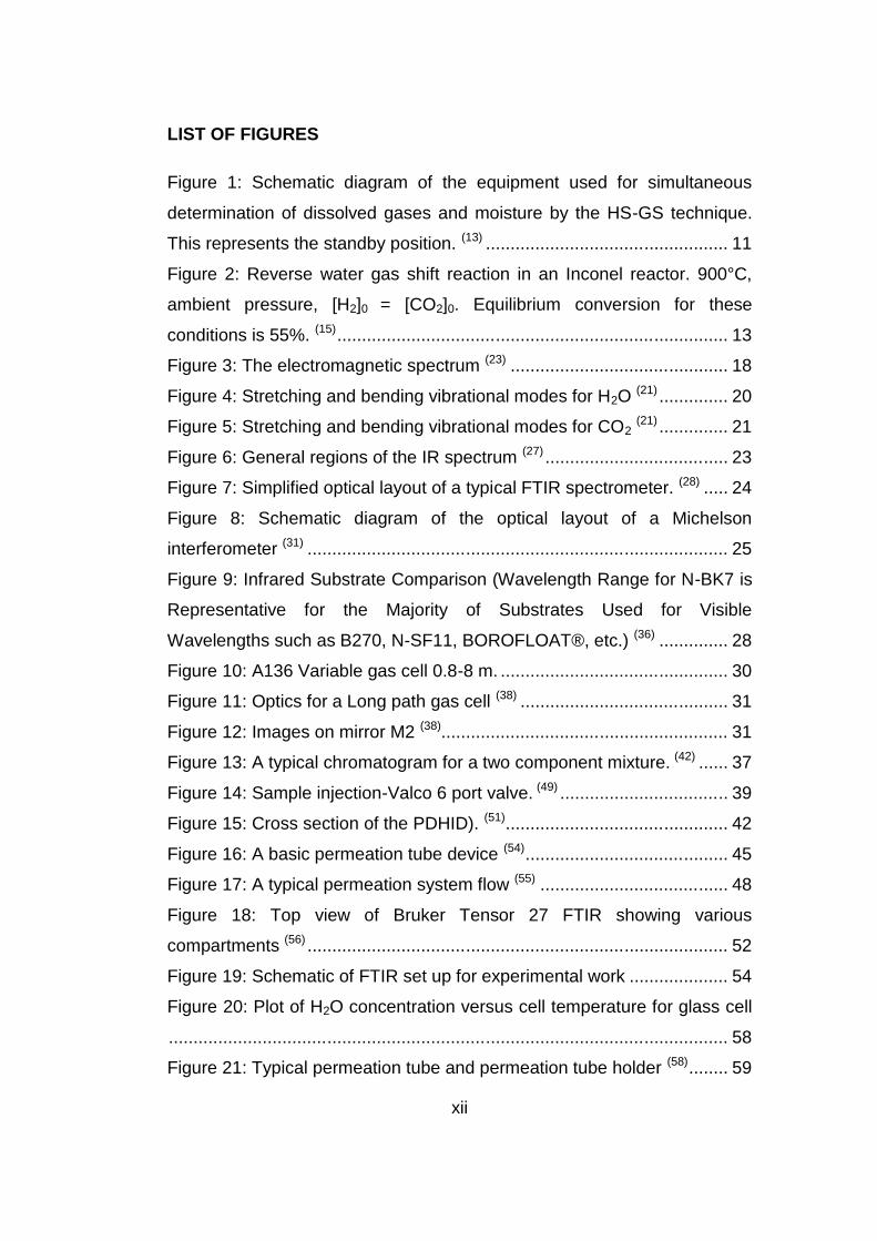
LIST OF FIGURES

Figure 1: Schematic diagram of the equipment used for simultaneous

determination of dissolved gases and moisture by the HS-GS technique.

This represents the standby position. (13) ................................................. 11

Figure 2: Reverse water gas shift reaction in an Inconel reactor. 900°C,

ambient pressure, [H2]0 = [CO2]0. Equilibrium conversion for these

conditions is 55%. (15)............................................................................... 13

Figure 3: The electromagnetic spectrum (23) ............................................ 18

Figure 4: Stretching and bending vibrational modes for H2O (21) .............. 20

Figure 5: Stretching and bending vibrational modes for CO2(21) .............. 21

Figure 6: General regions of the IR spectrum (27) ..................................... 23

Figure 7: Simplified optical layout of a typical FTIR spectrometer. (28) ..... 24

Figure 8: Schematic diagram of the optical layout of a Michelson

interferometer (31) ..................................................................................... 25

Figure 9: Infrared Substrate Comparison (Wavelength Range for N-BK7 is

Representative for the Majority of Substrates Used for Visible

Wavelengths such as B270, N-SF11, BOROFLOAT®, etc.) (36) .............. 28

Figure 10: A136 Variable gas cell 0.8-8 m. .............................................. 30

Figure 11: Optics for a Long path gas cell (38) .......................................... 31

Figure 12: Images on mirror M2 (38).......................................................... 31

Figure 13: A typical chromatogram for a two component mixture. (42) ...... 37

Figure 14: Sample injection-Valco 6 port valve. (49) .................................. 39

Figure 15: Cross section of the PDHID). (51)............................................. 42

Figure 16: A basic permeation tube device (54)......................................... 45

Figure 17: A typical permeation system flow (55) ...................................... 48

Figure 18: Top view of Bruker Tensor 27 FTIR showing various

compartments (56) ..................................................................................... 52

Figure 19: Schematic of FTIR set up for experimental work .................... 54

Figure 20: Plot of H2O concentration versus cell temperature for glass cell

................................................................................................................. 58

Figure 21: Typical permeation tube and permeation tube holder (58)........ 59

xiii

Figure 22: Typical FTIR spectra of H2O indicating peaks selected for

quantitation .............................................................................................. 61

Figure 23: Typical FTIR spectra of CH4 indicating peak selected for

quantitation .............................................................................................. 63

Figure 24: Spectrum obtained for Standard 1 .......................................... 66

Figure 25: Overlay of Standard 1 with a >94% C2H2 standard. The insert

shows a close up of the peaks at 1350 and 1305 cm-1. ........................... 66


Figure 27: Spectrum obtained on analysing Standard 2 using CH4 as

internal standard at 3017 cm-1. ................................................................ 69


Figure 29: Spectrum obtained on analysing Standard 3 with CH4 as

internal standard at 3017 cm-1. ................................................................ 71

Figure 30: In position A on the left, the sample loop is filled and in position

B on the right, the contents of the loop are injected onto the column. (59). 73

Figure 31: In position A on the left, the sample loop is loaded/column 1 is

backflushed and in position B on the right, the sample is sent to the

columns (60)............................................................................................... 74

Figure 32: In position A on the left, the sample loop is loaded in the initial

step and in the second step the heart cut is sent to the detector. In position

B on the right, the loop contents are sent to the column in the initial step

and in the second step the end cut is sent to waste. (61) .......................... 75

Figure 33: Sample holder for CaC2/H2O reaction..................................... 79

Figure 34: Linear calibration curve for moisture at 3854 cm-1 with a working

range between 0.514 and 9.890 ppm ...................................................... 81

Figure 35: Quadratic calibration curve for moisture at 3854 cm-1 with a

working range 0.514 to 9.890 ppm........................................................... 84

Figure 36: Linear calibration curve for CH4 at 3017 cm-1 with a working


Figure 37: Quadratic calibration curve for CH4 at 3017 cm-1 with a working


xiv

Figure 38: Linear calibration curve obtained for Standard 1 for C2H2 at

3313/3266 cm-1. ....................................................................................... 90


1305 cm-1 ................................................................................................. 90

Figure 40: Quadratic calibration curve obtained for Standard 1 for C2H2 at

3313/3266 cm-1. ....................................................................................... 92


1305 cm-1 ................................................................................................. 92


3313/3266 cm-1 ........................................................................................ 94


1350 cm-1 ................................................................................................. 94


1305 cm-1 ................................................................................................. 95


3313/3266 cm-1 ........................................................................................ 97


1350 cm-1 ................................................................................................. 97


1305 cm-1 ................................................................................................. 98


3313/3266 cm-1 using CH4 as internal standard..................................... 100


1350 cm-1 using CH4 as internal standard.............................................. 100









xv

Figure 54: Linear calibration curve for Standard 3 for C2H2 at 1313/3266

cm-1 with a working range between 94.804 and 291.265 ppm ............... 106

Figure 55: Linear calibration curve for Standard 3 for C2H2 at 1305 cm-1

with a working range between 94.804 and 291.265 ppm....................... 106

Figure 56: Linear calibration curve for Standard 3 for C2H2 at 1350 cm-1


Figure 57: Quadratic calibration curve for Standard 3 for C2H2 at

1313/3266 cm-1 with a working range between 94.804 and 291.265 ppm

............................................................................................................... 109

Figure 58: Quadratic calibration curve for Standard 3 for C2H2 at 1350 cm-1


Figure 59: Quadratic calibration curve for Standard 3 for C2H2 at 1305 cm-1










Figure 64: Examples of residual plots (62) ............................................... 117

Figure 65: Typical excel regression data. Red/bold data indicates

components used in calculations. .......................................................... 118

xvi

LIST OF TABLES

Table 1: FTIR window materials and properties (2) ................................... 29

Table 2: Label descriptions for Figure 18................................................. 52

Table 3: FTIR Settings ............................................................................. 56

Table 4: Dilution of moisture permeation standard to obtain calibration

levels........................................................................................................ 60

Table 5: Dilution of CH4 reference standard to obtain calibration levels .. 63

Table 6: Dilution of Standard 1 using mass flow controllers and nitrogen as

diluent ...................................................................................................... 65


diluent ...................................................................................................... 67

Table 8: Dilutions of Standard 2 using mass flow controllers and 9.9 ppm

CH4 standard in nitrogen as diluent ......................................................... 68


diluent ...................................................................................................... 69

Table 10: Dilutions of Standard 3 using mass flow controllers and 102 ppm

CH4 standard as diluent ........................................................................... 70

Table 11: Dilution of C2H2 standard using mass flow controllers ............. 77

Table 12: Summary of linear regression data for moisture standard:

Confidence intervals for the intercept....................................................... 81

Table 13: Summary of linear regression data for moisture standard:

Regression data for t test. ........................................................................ 82

Table 14: Summary of linear regression data for moisture standard: LOD

and LOQ values ....................................................................................... 83

Table 15: Summary of linear regression data for moisture standard: P

values ...................................................................................................... 83

Table 16: Summary of quadratic regression data for moisture standard:

Regression data for t test ......................................................................... 85

Table 17: Summary of quadratic regression data for moisture standard:

LOD and LOQ values............................................................................... 86

xvii

Table 18: Summary of quadratic regression data for moisture standard: P

values. ..................................................................................................... 86

Table 19: Summary of linear regression data for Standard 1 (C2H2):

Confidence intervals of the intercept. ....................................................... 91



Table 21: Summary of linear regression data for Standard 1 (C2H2): LOD

and LOQ values. ...................................................................................... 91

Table 22: Summary of linear regression data for Standard 1 (C2H2): P

values. ..................................................................................................... 91

Table 23: Summary of quadratic regression data for Standard 1 (C2H2):





LOD and LOQ values............................................................................... 93

Table 26: Summary of quadratic Excel regression data for Standard 1

(C2H2): P values. ...................................................................................... 93






and LOQ values. ...................................................................................... 96


values. ..................................................................................................... 96


Confidence intervals (no internal standard) ............................................. 98


Regression data for t test (no internal standard) ...................................... 98


LOD and LOQ values (no internal standard)............................................ 99

xviii

Table 34: Summary of quadratic regression data for Standard 2 (C2H2): P

values (no internal standard).................................................................... 99


Confidence intervals (with internal standard) ......................................... 101


Regression data for t test (with internal standard).................................. 101


and LOQ values (with internal standard)................................................ 102


values (with internal standard) ............................................................... 102






LOD and LOQ values (with internal standard) ....................................... 105




Confidence intervals (no internal standard) ........................................... 107


Regression data for t test (no internal standard) .................................... 107


and LOQ values (no internal standard) .................................................. 108


values (no internal standard).................................................................. 108


Confidence intervals (no internal standard) ........................................... 110


Regression data for t test (no internal standard) .................................... 110


LOD and LOQ values (no internal standard).......................................... 111

xix


values (no internal standard).................................................................. 111






and LOQ values (with internal standard)................................................ 113

Table 54: Summary of Linear regression data for Standard 3 (C2H2): P







LOD and LOQ values (with internal standard) ....................................... 115



Table 59: Comparison of moisture measurement techniques. ............... 126

1

CHAPTER 1: INTRODUCTION AND BACKGROUND

Introduction1.1.

In a number of specialty gas applications, the analysis of water vapor,

often referred to as moisture, is of high importance. The biggest driver for

the development and advancement of trace moisture analysis techniques

has, to date, been the microelectronics industry. The reason for this is that

even trace levels of water in process gases can affect device performance

and hence analytical techniques must be capable of detecting water vapor

from ppmv right down to sub-ppbv levels.

More than 50 different gaseous chemical components are used in the

production of various semiconductor devices. These are generally

classified by their handling and distribution as either bulk or specialty

gases. Bulk gases include nitrogen, oxygen, helium, argon and hydrogen,

all gases which are relatively inert and nontoxic. These gases are used for

purge procedures at large flow rates which include removal of residual

components from previous process steps or purging of ambient

components. (1)

The challenge of measuring water vapor at trace levels is largely due to

the adsorptive nature of the water molecule on metal and other surfaces.

In addition, the range of gas matrices that can potentially interfere with the

measurement process is huge and includes oxides, halides, hydrides,

corrosive gases, hydrocarbons and many more. Over the years a range of

techniques have been investigated as no single approach has been found

that can meet all the analysis requirements. These include Gas

chromatography (GC), mass spectrometry (MS), ion mobility spectrometry

(IMS) and spectroscopic methods such as Fourier Transform infrared

(FTIR), tunable diode laser absorption spectroscopy (TDLAS) and cavity

ring down spectroscopy (CRDS). (2)

2

This project initially started with the development of a FTIR method for

moisture analysis on Nitrogen Trifluoride (NF3) gas produced at NECSA by

the Pelchem plant facilities. The NF3 production facility at the Pelchem site

in Pelindaba, South Africa was constructed in the year 2000 with the

purpose of producing NF3, the primary uses of which included chamber-

cleaning gas in chemical vapor deposition semiconductor production

processes and in liquid crystal display production processes. NF3 is also

used as an etchant in semiconductor manufacturing and provides the

benefit of lower perfluorocarbon emissions as compared to alternate

cleaning gases. The NF3 facility at Pelchem was designed to supply

grades of product for each of the afore mentioned applications. One of the

Pelchem analytical specifications included low moisture content and a

method was developed in-house, using FTIR, to determine the moisture

content in NF3. The method utilized a BOMEM FTIR, a mercury cadmium

telluride detector (MCT) and a two meter corrosive resistant long path gas

cell. Method validation data sourced from internal validation documents

indicated that a method detection limit (LOD) of 0.4 ppmv had been

achieved for the measurement of moisture in NF3 matrix. (3) Later studies

performed at NECSA utilizing a similar system but with a ten meter gas

cell replacing the original two meter gas cell and a deuterated triglycine

sulphate detector (DTGS) and using helium as the matrix gas produced a

LOD of 1.77 ppmv. (4) The discrepancy in these two LOD’s could not be

explained adequately specifically as the helium method should have

produced a much lower LOD with the use of a longer gas cell path

although the DTGS detector is less sensitive than the MCT detector.

Many queries had previously been received at PAL requesting analyses

for moisture in various gas types and this together with the earlier

validation results obtained by the Pelchem group for moisture analyses in

NF3 and PAL’s results for moisture in helium led to the initiation of this

study.

3

Purpose of the study1.2.

The purpose of this project was to develop methods by which low parts per

million volume (ppmv) concentrations of moisture, specifically in gas

samples, could be analyzed. Initially analysis of moisture would be

performed using FTIR and a permeation standard. This method was to

serve as both a comparative and backup method. This was to be followed

by a process in which moisture present in gas samples was to be

converted to acetylene (C2H2) or carbon dioxide (CO2) and then analyzed

by FTIR and gas chromatography (GC). The C2H2 or CO2 results would

then be calculated back to moisture values.

Objectives of the study1.3.

The first objective of this project was the setup of a FTIR for moisture

analysis as both a comparative and backup method. For this method the

moisture was to be read directly on FTIR without conversion to C2H2 or

CO2.

The second objective of this project was the setup of a FTIR for C2H2 and

CO2 analysis. The purpose of this was to convert moisture in gas samples

into C2H2 or CO2 and analyzing using FTIR.

The third objective was the setup and optimization of a GC/ PDHID for

C2H2 and CO2 analysis. The purpose of this was to convert moisture in gas

samples into C2H2 or CO2 and analyzing using GC/PDHID.

The fourth objective was the design of a conversion system whereby the

moisture in gas samples could be converted, stoichiometrically, to either

C2H2 or CO2 prior to analysis using GC/PDHID or FTIR.

The fifth objective of this project was based on the success of the

conversion process. If the conversion was effective, method validation of

the conversion methods would be undertaken and the methods

implemented for commercial purposes in the laboratory.

4

Hypothesis

Hypothesis 1:

Is it possible to make use of an industrial process method to

stoichiometrically convert the moisture in a gas sample to an organic

compound such as C2H2 which is more readily analyzed on a GC than

moisture?

Hypothesis 2:

Is it possible to make use of an industrial process method to

stoichiometrically convert the moisture in a gas sample to a permanent

gas type such as CO2 which is more readily analyzed on a GC than water?

Hypothesis 3:

Is the analysis of C2H2 or CO2 more effective than the analysis of moisture,

due to the ingress of atmospheric moisture everywhere, using a FTIR as

the analytical technique?

Hypothesis 4:

Can parts ppmv levels of moisture be detected using a FTIR with an eight

meter path length glass cell and a MCT detector?

Importance of the study1.4.

A reliable and accurate method with which to measure moisture in gas

samples is required for a laboratory wishing to specialize in gas analyses.

Previous discussions with companies such as Afrox SA, who are currently

only able to reach concentration levels of 1 ppm and greater on their

moisture analyses in gas samples, led to the conclusion that this type of

analyses is an urgent requirement in the gas industry. Conversion of

moisture to acetylene should allow for small sample volumes to be used

and ppmv values to be achieved using GC/PDHID. Larger samples would

be required for FTIR analyses but in theory the conversion process should

5

be effective for these analyses using FTIR. Additionally it should be

possible to set up a FTIR method for the direct analyses of moisture in the

ppmv ranges although this method would require large amounts of sample

as cell conditioning for moisture takes much longer than for an organic

compound such as C2H2.

6

CHAPTER 2: LITERATURE REVIEW

Introduction and background2.1.

Precise analysis of natural gas is important for determining the price,

calorific value, identification of source and gas quality. In natural gas there

are a number of components from C1 to C10 hydrocarbons, including

isomers. Their physical properties are similar and the composition ratio of

major to minor components is high, making quantification by ordinary

analytical means difficult. Two analytical methods most frequently used in

the industry are ASTM D-1945 and GPA standard 2261 multi-column

technique. These methods encompass the use of a ten port valve, two six

port valves and several columns. Recently a simpler technique using an

alternative system with two gas chromatographs (GC-GC) and four

columns was introduced. In this system the first GC is equipped with a

thermal conductivity detector (TCD) and a flame ionization detector (FID)

and the second GC is equipped with a TCD and a flame photometric

detector (FPD). The FID was used to characterize hydrocarbons, the TCD

for permanent gases such as oxygen, nitrogen, carbon dioxide and the

FPD for sulfur components. Using these combined techniques, a complex

mixture of C1 to C10 hydrocarbons, permanent gases and sulphur

compounds could be well characterized with good resolution and

repeatability. (5)

Afore mentioned systems addressed the analyses and characterization of

natural gas components and set the benchmark for this type of analyses.

However, the detection limits obtained for these methods do not meet the

requirements of the semiconductor industry where trace levels of

impurities in high purity gases need to be determined. Quantification of

trace levels was made possible by the introduction of the pulsed discharge

helium ionization detector (PDHID) in 1992. (6) It provided advantages with

simple configuration, convenience, high sensitivity and good versatility. As

helium passes through the ionization chamber, the analyte(s) eluting

7

through the GC capillary column are ionized by the helium metastables

and photons and transfer the signal to the electrometer. Since the

ionization potential of the metastable helium is higher than that of all

species, with the exception of the argon ion, all other compounds can thus

be ionized by the helium. For this reason the PDHID has become the most

universal detector, capable of detecting H2, O2, CO2, H2O as well as a

variety of organic compounds ranging from light hydrocarbons to high

molecular weight pesticides and metal complexes. Its sensitivity towards

hydrocarbons is in the order of 1 pg s-1. (5) Introduction of the PDHID meant

that the TCD and FID could effectively be replaced by one detector thus

eliminating the complexities of using two different detectors.

According to Roberge et al, (7) a PDHID was used, under appropriate

separation conditions, to detect hydrogen and methane from the matrix

components of human breath samples. The sensitivity of this method is

over an order of magnitude better than published methods using a FID

and a TCD and has an additional advantage of detecting both analytes

with only one detector. Limits of detection (LOD) were 0.3 ppm for both

hydrogen and methane and the method had a linear dynamic range (LDR)

of three orders of magnitude (0.3 – 400 ppm, v v-1). The PDHID was also

compared to the FID and TCD with regards to selectivity, sensitivity and

reproducibility for high-speed gas chromatography (HSGC). It was shown

that the PDHID is as sensitive as the FID for fast separations but was

limited by the difficulty of resolving analyte peaks from O2 and N2 matrices.

The PDHID was at least three orders of magnitude more sensitive than the

TCD for all analytes examined (7)

Although the PDHID allowed for simplification of the analytical method and

detection at low concentrations, other problems were encountered with the

determination of trace impurities in pure gases. GC/PDHID systems with

packed columns are commonly used in this role because of their universal

detection capability and high sensitivity. The challenge of this analysis is

8

the difficult separation and quantitation of trace impurities often eluting

adjacent to or within the peak of the main component/matrix. One solution

is the removal of the matrix by separators but this is only applicable for a

limited number of gases and is often not cost effective due to the limited

lifetime of the separators. Additionally, interference between the separator

and gas molecules has been observed. An alternative method is the use

of multiple capillary columns and column switching techniques. The

separation of the trace impurities and the matrix was also improved by the

use of capillary columns in place of packed column. However, the matrix

still flowed through the analytical column to the detector saturating both

the columns and PDHID with the matrix. In addition, trace levels of

impurities remained embedded in the shoulder of the matrix peak making

detection and quantitation difficult (8)

A unique system was designed by which the trace impurities were

separated from the matrix in a pre-column by venting the matrix before the

target compounds eluted. The trace impurities (together with a small

portion of the matrix) were then transferred onto a second column for

further separation. This technique, referred to as “heart cutting and back

flushing”, was employed on a system equipped with three two-position

valves, a two way solenoid valve and four packed columns. This

configuration enabled detection and quantitation of trace impurities without

interference from peak tailing by the matrix. This method has been applied

to H2, Ar and N2 respectively. A method detection limit of 100 nl l-1 was

achieved and a dynamic range of 100 - 1000 nl l-1 was obtained for

methane in argon (8)

Now that it has been determined that it is possible to analyze effectively for

various components such as permanent gases and hydrocarbons at trace

levels in high purity gases, the question arises “How to analyze effectively

for trace levels of moisture in high purity gases?”

9

Fourier Transform Infrared (FTIR) spectroscopy is an analytical method

that can be optimized for the analysis of corrosive gases and in addition is

capable of detecting low ppb levels of water vapor. The detection limit of

FTIR spectroscopy combined with classical least squares multivariate

calibration is about 20 ppb when using a one meter path length cell and a

one minute collection time. Longer collection times or a longer path length

cell will provide greater sensitivity but both these options will result in

slower measurement speeds. The user can thus trade off speed for

sensitivity depending on individual situations. (9)

An infrared method for the measurement of the moisture content of

hydrocarbons in the ppmv range was developed using the conversion of

moisture to C2H2 with calcium carbide (CaC2) followed by a subsequent

transfer, using a dry carrier gas, of the C2H2, to the infrared cell where it

was re-dissolved into carbon tetrachloride and measured. The reason for

the conversion of the moisture to C2H2 in the hydrocarbon was to eliminate

background absorption by the hydrocarbon. (10)

Other instrumental methods currently being used, or in development, for

measuring trace moisture at ppbv levels include tunable diode laser

absorption spectroscopy (TDLAS), cavity ring-down spectroscopy (CRDS)

and intracavity laser spectroscopy (ILS). In addition, sensor-based

technologies such as oscillating quartz crystal microbalances, chilled

mirror-, capacitor-, and electrolytic-based hygrometers operate in this

area. The success of each trace moisture method is dependent on the

degree to which the different process gases interfere with the

measurement process.

Very few references were found with regards to the analysis of moisture

using gas chromatography. R.P. Badoni and A. Jayaraman (11) analyzed

for moisture using a gas chromatograph coupled to a Thermal Conductivity

Detector (GC/TCD) but this was only really effective for water contents

greater than 50%. California Environmental Protection Agency (CEPA)

10

brought out a standard operating procedure (SOP) for the determination of

moisture in consumer products using a GC/TCD. (12) This method has a

detection limit of 1.0 mg ml-1.

J. Albert et al (13) developed a method whereby mineral oil was analyzed

for dissolved gases, H2, O2, N2, CO, CO2, CH4, C2H6, C2H4, C2H2 and

C3H8, using static headspace capillary gas chromatography (HSGC). High

voltage transformers are susceptible to malfunctions such as arcing,

overheating and partial discharges, which always result in the chemical

decomposition of the mineral oil and cellulose insulation. Several gases,

totally or partially dissolved in the oil, are produced. A headspace sampler

device was used to equilibrate the sample species in a two phase system

under controlled temperature and agitation conditions. A portion of the

equilibrated species was then automatically split-injected into two

chromatographic channels mounted on the same GC for separation. The

hydrocarbons and the lighter gases were separated on the first channel by

a GS-Q column coupled with a Molsieve 5-A column via a bypass valve,

while the moisture was separated on the second channel using a

Stabilwax column. The analytes were detected using two PDHID’s. The

performance of the method was established using equilibrated vials

containing known amounts of gas mixture, water and blank oil. Detection

limits for the method were established between 0.08 µl l-1 and 6 µl l-1 for

the dissolved gases, excluding O2, N2 and CO2 where higher values were

observed mostly due to air ingress during sampler operations, and

detection limits of 0.1 µg g-1 were established for the dissolved water. Ten

consecutive measurements in the high and low levels of the calibration

curves showed a precision better than 12% and 6% respectively in all

cases. Figure 1 below depicts the experimental setup for this process.

11

Figure 1: Schematic diagram of the equipment used for simultaneousdetermination of dissolved gases and moisture by the HS-GS technique. Thisrepresents the standby position. (13)

The FTIR is an obvious choice as there are currently methods available for

this technique with regards to moisture analysis and these go down to ppb

levels. (9) The drawback of FTIR is that a fairly large amount of sample is

required for the analysis and this is not always available.

Since a PDHID is 500 times more sensitive than a TCD and 50 times more

sensitive than a FID (8), why not consider this as an option for moisture

analysis? The PDHID is a universal detector and can be used for the

analysis of certain gases that cannot be detected by an FID e.g. O2, N2,

Ar, CO and CO2 and its sensitivity makes it a potentially better choice than

a TCD.

The drawback to the PDHID is that exposure to moisture adversely affects

its performance. This leads to an alternative suggestion and the pivot on

which this proposal is based.

12

Was it possible to convert the moisture, at whatever levels present in a

gas sample, to an alternative component that can be effectively analyzed

by a PDHID? Two industrial processes are to be considered for this

proposal:

Acetylene production

Calcium carbide is produced industrially in an electric arc furnace from a

mixture of lime and coke at approximately 2000°C. The reaction is as

follows:

CaO + 3C → CaC2 + CO (1)

One of the applications that CaC2 is used for industrially is the production

of acetylene. The reaction was discovered by Friederich Wöhler (14) in

1862 and the reaction equation is as follows:

CaC2 + 2H2O → C2H2 + Ca (OH) 2 (2)

This reaction is the basis of the industrial manufacture of acetylene and is

the major industrial use of calcium carbide.

The question arose “Is it possible to make use of this equation to design a

reaction vessel, containing calcium carbide which can be forced to react

stoichiometrically with moisture from a gas sample, at room temperature,

to produce acetylene which can then be analyzed using a GC/PDHID

system.

Water gas shift r eaction

Another industrial application which may allow for the conversion of

moisture to a compound easily analyzed by GC is the water gas shift

reaction (WGSR).

The WGSR is an important industrial reaction for the production of

chemicals and/or hydrogen. It is an exothermic, equilibrium limited reaction

that shows decreasing conversion with increasing temperature. A catalyst

13

is required at temperatures below 600°C because of the lower reaction

rate at low temperatures. (15) The reaction equation is as follows:

CO + H2O → CO2 + H2 ΔH = -41.1 kJ mol-1 (3)

Bustamante et al (15) experimented with both Inconel (mixture of 72%

Nickel, 17% Chromium and 10% Iron) and quartz reactors and found that

conversions were very high for small residence times and that these

conversions were two orders of magnitude greater using the Inconel

reactor compared to the quartz reactor. The result implied that the metal

walls of the Inconel reactor catalyzed the reaction. See figure 2 below.

Figure 2: Reverse water gas shift reaction in an Inconel reactor. 900°C, ambientpressure, [H2]0 = [CO2]0. Equilibrium conversion for these conditions is 55%. (15)

According to A. Luengnaruemichai et al (16) there are two types of WGSR

catalysts which are used commercially. The high temperature shift catalyst

is made up of oxides of iron and chromium and is used between 400 -

500°C and will reduce the carbon monoxide to between 2 - 5%. The

second catalyst, which is the one being considered for this project, is a low

14

temperature shift catalyst composed of copper, zinc oxide and alumina

and is used between 200 - 400°C to reduce the carbon monoxide

concentration to about 1%. The thermodynamics of the WGS reaction are

well known in that at high temperatures the conversion is equilibrium

limited and at low temperatures it is kinetically limited. Commercially, a

combination of the two catalysts is used with in-between cooling. If more

active low temperature shift catalysts can be found, the conversion can

then approach the equilibrium limit more closely. (15) The question is

whether these catalysts can be used together with the water gas reaction

to produce stoichiometric amounts of carbon dioxide and/or hydrogen from

a gas sample containing moisture, both of which can be analyzed using

GC/PDHID.

Methods for moisture analysis2.2.

A number of methods have evolved over the years with regards to

moisture analyses. The method most commonly used is the gravimetric

drying process which is the most basic and most time consuming of all the

available methods. It is also restricted as it principally determines loss on

drying and not necessarily the water content. Apart from water, other

volatile components of the sample and/or decomposition products are also

determined.

Titration methods, in contrast to drying methods, are very specific. Karl

Fischer developed the KF titration with which both bound and free water

can be determined. The method works over a wide range of

concentrations from ppm to % levels. It is based on the Bunsen Reaction,

used for the determination of sulfur dioxide in aqueous solutions:

SO2 + I2 + 2H2O → H2SO4 + 2HI (4)

In modern synthetic chemistry dehydration procedures are often

performed to ensure experimental reproducibility when water sensitive

reagents are used. Despite these precautions, water’s pervasiveness,

15

solubility and propensity to physisorb on reaction vessel surfaces lead to

the question “How dry is dry” and this proves difficult to answer if an

accurate determination of trace water contaminant at the µg level is

required. (17) Sun et al (17) have developed a method where the potent

dehydrating ability of difluoro(aryl)- λ3-iodanes is exploited to develop a

convenient 19F-NMR-based aquametry method that is more sensitive than

coulometric Karl Fischer titration.

Chemical processes involving moisture2.3.

The Water Gas Shift Reaction (WGSR) is a reaction traditionally used for

the production of Hydrogen (H2) from synthesis gas. The hydrogen is then

used for ammonia production in the fertilizer industry, for a variety of

operations in the refinery industry and more recently as fuel for power

generation and transportation. The reaction is expressed as follows:

CO + H2O ↔ CO2 + H2 ΔH0298K = - 41.09 kJ mol-1 (5)

The reaction is a moderately exothermic, reversible reaction. The catalyst

used initially contained iron and chromium and was capable of catalyzing

the reaction at 400 to 500°C and it reduced the exit carbon monoxide

content to about 3%. The equilibrium constant for the reaction decreases

with increasing temperature. The reaction is thermodynamically favored at

low temperatures and kinetically favored at high temperatures. The

reaction is also not affected by pressure as there is no change in volume

from reactants to products. (18)

Both metals and metal oxides can be used to catalyze the WGSR.

Catalysts are classified into two categories namely “High Temperature

Shift” catalysts and “Low Temperature Shift” catalysts. The “High

Temperature Shift Catalysts are typically an iron oxide chromium oxide

catalyst which functions in the range of 310 to 450°C and produce an exit

composition of carbon monoxide (CO) at 2 to 4% as the temperature

increases but at lower temperatures these catalysts lose their activity. The

16

“Low Temperature Shift” catalysts are typically copper based catalysts

which function at 200°C and can achieve exit composition of CO

concentrations at 0.1 to 0.3%. Commercially the WGSR is carried out in

two adiabatic stages namely the high temperature shift followed by the low

temperature shift with inter-cooling to maintain the inlet temperature. This

configuration is necessary as the copper based catalyst is easily poisoned

by sulphur compounds coming off the coal or hydrocarbon sources used

while the iron based catalysts are sulphur tolerant. Both types of catalysts

are commercially available. (18)

Acetylene was once a major raw material used for the production of

synthetic chemicals such as vinyl chloride, vinyl acetate, acrylonitrile and

acetaldehyde. In the mid 1960’s, however, acetylene use began to be

replaced by ethylene produced from low cost petroleum. Today the major

chemical applications for acetylene are for the production of vinyl chloride

monomer and 1, 4 butanediol. Non chemical applications include welding

and cutting of metals and the production of carbon for batteries. In the

United States, the majority of acetylene produced is used as chemical

feedstock. It is difficult to transport and is generally used at or near its

production site because of its high flammability and combustion heat. (19)

Pure acetylene is a colorless, odorless gas. Technical grade acetylene has

garlic like odor, attributable to contamination by impurities. Some of these

impurities include divinyl sulfide, ammonia, phosphine, arsine, methane,

hydrogen sulphide and many others. (20)

A number of high temperature processes for the production of acetylene

have been commercialized via cracking reactions in the 1000 to 1600°C

temperature range or synthesis reactions at temperatures above 1600°C.

These include a number of processes such as partial oxidation where

methane, LPG or light gasolines are pyrolized to cracked gases containing

acetylene, electric or plasma arc whereby light hydrocarbons are cracked

into acetylene using an electric arc and the calcium carbide process where

17

acetylene is generated by the reaction between calcium carbide and

water.

The classical commercial route to acetylene is the calcium carbide route in

which lime is reduced by carbon (in the form of coke) in an electrical

furnace to yield calcium carbide:

CaO + 3C → CaC2 + CO (6)

The calcium carbide is then hydrolyzed to produce acetylene:

CaC2 + 2H2O → C2H2 + Ca (OH) 2 H = -129 kJ_mol-1 (7)

There are two principal methods for producing acetylene from calcium

carbide and these are based on the type of generator used. In the wet

generator, the reaction takes place in a cylindrical water shell attached

below a carbide feed hopper. The carbide is fed into the water reservoir at

a controlled rate until the reaction has run to completion. Calcium

hydroxide is obtained as a byproduct in a slurry form containing 10 to 20%

hydroxide. For larger scale plants, the dry generation design is more

common. This design features a continuous feed of carbide mixed with

sufficient water to complete the reaction as well as dissipate the heat

generated by the reaction. Typically, a kg of water is used per kg of

carbide. The reaction heat is dissipated by water evaporation, leaving a

residue of powdered calcium hydroxide with a moisture content of 1 to 6%.

Both processes yield acetylene with approximately 99.6% purity by volume

after a light scrubbing. (19)

Infrared spectroscopy2.4.

Introduction

Infrared spectroscopy is one of the most common spectroscopic

techniques used by organic and inorganic chemists. A sample is

positioned in the path of an IR beam and its absorption of various IR

frequencies is measured. This enables determination of the different

18

chemical functional groups in the sample, as each functional group type

absorbs characteristic frequencies of IR radiation. Infrared spectroscopy

allows for the analysis of gases, liquids and solids making it a versatile and

popular technique with which to determine structural elucidation as well as

compound identification. (21) However, since FTIR functionality is based on

the principle that almost all molecules absorb infrared light, monoatomic

gases such as He, Ne, Ar and homo-polar diatomic molecules such as H2,

N2 and O2, all of which do not absorb infrared light as they do not have

dipolar moments, cannot be analyzed or identified using infrared

spectroscopy. (22)

The term “electromagnetic spectrum” refers to the collection of radiant

energy which stretches from cosmic rays to X-rays to visible light to

microwaves. Each of these can be considered as wave or particle

travelling at the speed of light and each of these waves differ from each

other with respect to length and frequency. (21) See Figure 3 below.

Figure 3: The electromagnetic spectrum (23)

19

Frequency refers to the number of wave cycles that pass through a point

in one second. It is measured in Hertz (Hz) where 1Hz = 1 cycle sec-1.

Wavelength is the length of one complete wave cycle. It is measured in

centimeters (cm). Wavelength and frequency are inversely related as

indicated below: (21)

ʋ = c / ʎ and ʎ = c / ʋ (8)

Where:

c = speed of light (3 x 1010 cm sec-1

ʋ = frequency in Hz

ʎ = wavelength in cm

Energy is related to wavelength and frequency as follows:

E = hʋ = hc/ ʎ (9)

Where: h = Plank’s constant (6.6 x 10-34 joules sec-1)

The infrared section of the electromagnetic spectrum is divided into three

regions namely the near, mid and far infrared regions. Near-IR is a high

energy region (14000 – 4000 cm-1 or 0.8 – 2.5 µm wavelength) which can

excite overtone or harmonic vibrations. The mid-infrared (4000 – 400 cm-1

or (2.5 – 25 µm) is used to study the fundamental vibrations and

associated rotational-vibrational structure while the far-infrared (400 – 10

cm-1 or 25-1000 µm) has low energy and is used for rotational

spectroscopy. (24)

Theory of infrared absorption

All atoms that are in a bonded state tend to vibrate. The only time vibration

does not occur is when an atom in the bonded state is at zero degrees

Kelvin. These vibrations typically take place at 10-15 seconds. Infrared

spectrometry analyzes the number of infrared photons as well as the

20

amount of energy present in infrared photons absorbed by the molecule.(25)

Absorption of IR is only possible in compounds with small energy

differences in the possible vibrational and rotational states. A molecule will

only absorb IR if the vibrations or rotations within the molecule cause a net

change in the dipole moment of the molecule. Electromagnetic radiation is

made up of oscillating electrical and magnetic fields which are

perpendicular to each other. The electrical field of the radiation interacts

with fluctuations in the dipole moment of the molecule and if the frequency

of the radiation matches the vibrational frequency of the molecule, then

radiation is absorbed and the amplitude of molecular vibration changes.(26)

Molecular vibrations are classified into two types, stretching and bending.

A molecule made up of n atoms has a total of 3n degrees of freedom

which corresponds to the Cartesian coordinates of each atom in the

molecule. In a nonlinear molecule, 3 of these degrees are rotational and 3

are translational and the rest correspond to fundamental vibrations, while

in a linear molecule, 2 degrees are rotational and 3 are translational.

Therefore a nonlinear molecule has “3n-6” degrees of freedom and a

linear molecule has “3n-5” degrees of freedom. (21)

Water is a nonlinear molecule and has three fundamental vibrations

indicated below in Figure 4.

Figure 4: Stretching and bending vibrational modes for H2O (21)

21

Carbon Dioxide is a linear molecule and therefore will have four

fundamental vibrations as seen in Figure 5 below.

Figure 5: Stretching and bending vibrational modes for CO2(21)

A molecule has a number of vibrational energy states, the lowest being the

ground vibrational state and anything above that is referred to as an

excited vibrational state. When a molecule absorbs a photon of light, it

gains energy and moves from ground state to an excited state. This is not

a physical movement as such but rather an increase in the average bond

length of the molecule. Atoms in a molecule undergoing stretching will

move further apart while atoms in a molecule that is bending will undergo

a change in the bending angle when photon absorption occurs.

Since vibrational state energies are quantized, a molecule can only absorb

specific photons with specific energies in an attempt to change its

vibrational energy state. The following equation is used to calculate the

change in energy between two vibrational states: (25)

ΔE = hʋ (10)

Where:

ΔE = change in energy between two vibrational states

ʋ = frequency of the photon (cm-1)

22

h = Planck’s constant (6.626 x 10-34 Hz)

IR stretching frequencies are controlled by the functional group and for this

reason IR spectrometry can be used to determine which functional groups

are present or absent in a molecule. The stretching frequency can be

explained by Hooks Law which relates to the manner in which masses on

a spring behave. The atoms in a molecule can be regarded as mass

pieces and the bond between the atoms as a spring, and the greater the

number of electrons shared between the atoms, the greater the resistance

of the atoms to being pulled apart. Thus the higher the bond order, the

higher the spring stiffness and the higher the stretching frequency. (25)

The energy change between molecular vibrational states is based on the

bond order and the masses of the bonded atoms. Functional groups are

described by the bond order and the masses of the bonded atoms.

Functional groups in a molecule can therefore be predicted by recognizing

common patterns of IR absorption i.e. the amount and wave number of

photons. (25)

The general regions of the infrared spectrum in which various kinds of

vibrational bands are observed are outlined in Figure 6 below. The blue

colored sections refer to stretching vibrations and the green colored bands

indicate bending vibrations. The infrared spectra in region of 1450 to 600

cm-1 is generally very complex making it difficult to assign all absorption

bands but due to the unique patterns found in this region, it is often

referred to as the fingerprint region. Absorption bands in the 4000 to 1450

cm-1 are usually due to stretching vibrations of diatomic units and this is

often referred to as the group frequency region. (27)

23

Figure 6: General regions of the IR spectrum (27)

Instrumentation

Dispersive spectrometers were introduced in the mid 1940’s and were

later followed by FTIR spectrometers. A FTIR spectrometer is able to

collect all wavelengths simultaneously unlike the dispersive instrument

which collects each wavelength sequentially. (28) FTIR spectrometry is a

technique based on the interference of radiation between two beams, to

provide an interferogram. An interferogram is defined as the signal

produced as a function of the change of path length between the two

beams. (29)

A FTIR system is made up of three basic components, a radiation source,

an interferometer and a detector as per Figure 7.

24

Figure 7: Simplified optical layout of a typical FTIR spectrometer. (28)

Interferometer

The most commonly used interferometer is the Michelson interferometer

(See Figure 8). The interferometer consists of a beam splitter, a fixed

mirror and a moving mirror. (30) The mirrors are perpendicular to each

other. (28) The beam splitter is made of a material which transmits half the

radiation striking it and reflects the other half. Typically a beam splitter is

made by depositing a thin film of germanium onto a flat potassium bromide

(KBr) substrate. (28) Radiation from the source strikes the beam splitter and

separates into two beams. One beam is transmitted through the beam

splitter to the fixed mirror and the second is reflected off the beam splitter

to the moving mirror. (30) A path difference between the beams is

introduced and the beams are then recombined. In this way, interference

between the beams is obtained and the intensity of the output beam from

the interferometer can be monitored as a function of path difference using

an appropriate detector. (31)

25

Figure 8: Schematic diagram of the optical layout of a Michelson interferometer(31)

Radiation source

FTIR spectrometers make use of a Globar or Nernst source for the mid-

infrared region. A high pressure mercury lamp is used for the far-infrared

region and tungsten-halogen lamps are used as sources for the near-

infrared regions. (29)

The Nernst glower is able to reach temperatures of up to 1500°C. It is

made up of a fused mixture of oxides of zirconium, yttrium and thorium,

molded into hollow rod shapes, approximately 1 - 3 mm in diameter and 2

- 5 cm in length. The rod ends are cemented to short ceramic tubes for

easy mounting and short platinum leads provide power connections.

Nernst glowers must be preheated to be conductive as they have a

negative coefficient of resistance. They therefore require auxiliary heaters

as well as a ballast system to prevent overheating. The energy output is

predominantly concentrated between 1 and 10 µm, with relatively low

26

energy beyond 10 µm. Radiation intensity is double that of a Globar

source with the exception of the near-infrared region. (32)

A Globar typically has intermediate characteristics between heated wire

coils and the Nernst glower. In comparison to the Nernst glower, the

Globar is a less intense source below 10 µm, comparable between 10 to

15 µm and superior beyond 15 µm. It is made up of a silicon carbide rod, 6

- 8 mm in diameter, is self-starting and has an operating temperature of

approximately 1300°C. In contrast to the Nernst glower, the Globar has a

positive temperature coefficient of resistance and can be controlled with a

variable transformer. The resistance of a Globar increases with time and

provision must therefore be made for increasing the voltage across the

unit. The spectral output of the Globar is roughly 80% that of a blackbody

radiator. (32)

Detector

Infrared detectors are classified into two types namely thermal and photon

detectors. With photon detectors, radiation is absorbed within the material

by interaction with electrons. The changed electronic energy distribution

results in an electrical output signal which can be detected. Photon

detectors are advantageous in that they show a selective wavelength

dependence of the response per unit incident radiation power, have

perfect signal to noise performance and a very quick response. The

disadvantages of these detectors are that they require cryogenic cooling

making them bulky and tedious to use. (33)

Thermal detectors, in contrast to photon detectors, absorb incident

radiation to change the temperature of the material, resulting in changes in

physical properties which generate an electrical output. Thermal effects

are generally independent of wavelength and depend on the radiant power

and not on spectral content. Thermal detectors typically operate at room

temperatures and are usually characterized by modest sensitivity and a

response slower than that of the photon detectors. (33)

27

The photon type detector of choice for this project was the Mercury

cadmium telluride (MCT) detector so named for the mercury/telerium and

cadmium/telerium detection element it contains. Because of its high

response speed, there is no change in sensitivity with the standard mirror

speed making this detector suitable for applications that require

measurement over a short period of time. In addition, an MCT detector has

a D* value at least ten times larger than that obtained by a thermal

detector. The D value is an indicator of performance and is defined as

follows: (34)

D = 1/NEP [Hz1/2/W] and (11)

D* = D/A1/2 [cm Hz1/2/W] (12)

Where NEP is defined as noise equivalent power and is the incident power

that gives signals for which the S/N ratio is 1. Signals smaller than 1

cannot be detected indicating that the lower the NEP of a detector, the

more efficient its S/N characteristics are. Because the D* value of the MCT

detector is larger than that of a thermal detector, it’s suitable for

measurements associated with low levels of intensity such as

measurements performed with long-path gas cells. High levels of light

intensity on the other hand, may cause false peaks in the region below

650 cm-1 as there will be a nonlinear relationship created between the light

incident on the detector and the output voltage. In this case, the light

intensity will need to be reduced by for example, changing the aperture

settings. (34)

Windows

The flow path of the sample in a FTIR system is fairly simple up to the

point where the sample gas comes into contact with such parts as the O-

rings, gas cell, optical windows and mirrors. The material for the windows

and its transmission range determines the output for the detector. See

28

Figure 9. The correct window for the required application must be able to

withstand the chemical environment while simultaneously having a wide

enough transmission range for the selected analysis. (2)

There are many types of infrared window materials to choose from and

each type has its own characteristics. The most pertinent points to

consider when choosing infrared windows are the following: spectral

range, chemical properties of the sample versus that of the window,

physical properties of the window and costs. (35)

Figure 9: Infrared Substrate Comparison (Wavelength Range for N-BK7 isRepresentative for the Majority of Substrates Used for Visible Wavelengths suchas B270, N-SF11, BOROFLOAT®, etc.) (36)

29

Table 1: FTIR window materials and properties (2)

MaterialDescription

ChemicalName

Transmissionrange (cm-1)

RefractionIndex Description

AMTIR-1 Ge-As-Se 13,333-714 2.606 Insoluble in H2O;Expensive

BariumFluoride BaF2 50,000-869 1.46

Sensitive to thermal shock;insoluble H2O;resistant tofluorine and fluorides

CalciumFluoride CaF2 66,667-1,111 1.40

Low solubility; insoluble inH2O;resistant to most acidsand alkalides; not to beused with NH3 salts

Cesium Iodide CsI 6,667-200 1.74 Hygroscopic; easilyscratched

Germanium Ge 5,000-869 4.0 Chemically inert; hard andbrittle and tends to fracture

MagnesiumFluoride

MgF2 90,909-1,333 1.37-1.38 More soluble than CaF2;sensitive to thermal shock

PotassiumBromide KBr 40,000-400 1.53

Low cost; extendedtransmission range;withstands thermal andmechanicalshock;hygroscopicPotassium

Chloride KCl 55,555-500 1.46Less hygroscopic andmore resistant to thermalshock than NaCl

Silicon dioxide SiO2 25,000-2,500 1.5a Insoluble in water;birefringent

Silver Bromide AgBr 20,000-300 2.2Insoluble; will cold flow;darkens less than AgCl inUV light

Silver Chloride AgCl 25,000-434 2.0 Soluble in H2O; corrosiveto metals

SodiumChloride

NaCl 40,000-667 1.52 Low cost; rugged;hygroscopic

Thalliumbromoiodide(KRS-5)

TlBr-TII 20,000-285 2.37Soluble in bases; insolublein acids; slightly H2Osoluble

Zinc Selenide ZnSe 10,000-556 2.40Insoluble in H2O; resistantto most solvents; brittle;handle with caution

Zinc Sulfide ZnS 10,000-714 2.20Insoluble in H2O; slightlysoluble in nitric acid,sulfuric acid and potassiumhydroxide

a At 333 cm-1

Long Path Gas Cell

Gas cells used for gas analyses in FTIR analytical systems generally have

path lengths ranging from 2 to 10 m. High sensitivity is the greatest

30

advantage provided by a 10 m cell but this is offset against the very large

sample volumes, generally about 2 liters, required for analyses. (37)

Short path gas cells are generally used to measure gases at high

concentrations while long path gas cells are used to measure gas

concentrations down to the part per billion levels. For the purpose of this

study, a long path gas cell was used to obtain the ppm levels of moisture

required. See Figure 10 below.

Figure 10: A136 Variable gas cell 0.8-8 m.

A gas cell having a 10 or 20 m path length contains at least three mirrors

and the long light path is achieved by repeated reflections of the light

along the mirrors within the gas cell. The three mirrors shown in figure 11

each have an identical radius of curvature which provides the base light

path length of the gas cell. Infrared light from the light source is focused on

the inlet port of the gas cell. It is then reflected from mirror M1 and focuses

31

on mirror M2. The infrared light from M2 is then reflected from mirror M3

and focuses back onto mirror M2.(38)

Figure 11: Optics for a Long path gas cell (38)

Figure 12 indicates the images formed on mirror M2. It is made up of two

levels namely 4n-2 and 4n (where n is a natural number) which show the

sequence numbers of the images formed on mirror M2. The infrared red

light is reflected multiple times between mirrors M1, M2 and M3 and is

finally reflected from mirror M3 to be focused on the exit port before

reaching the detector.

Figure 12: Images on mirror M2 (38)

32

To determine trace amounts of analyte Beers-Lambert-Bouguer’s Law is

put into practice. It states that the absorbance is directly proportional to the

absorptivity of the analyte, its concentration and the path length of the cell,

A = α*b*C (13)

Where:

A = Absorbance

α = absorptivity in units of length -1 concentration-1 (e.g. m-1 M-1)

b = Path length of the cell in units of length

C = Concentration in Molarity or g mol-1

Each absorption, seen within a spectrum, may be assigned to a vibrational

mode within the molecule and each has its own contribution to the

absorptivity term α. Absorbance is then determined from the primary

measurement as follows: (39)

A =log (1/T) = -log10T (14)

Where: A = Absorbance

T = Transmittance

The longer the path length at a fixed concentration, the greater the number

of molecules the IR beam will pass through. In practice however, there is

the competing process of increasing noise as the IR signal is reduced by

mirror reflection losses as well as losses due to scattering. An acceptable

number of reflections in a multi pass gas cell is approximately 40

reflections with a standard white cell and approximately 80 using a

modified Horn Pimentel gas cell design. The purpose is to increase the

path length at a rate which is quicker than that with which the noise

increases. (40)

33

Measurement of gas samples on FTIR

In a solid or liquid sample, the molecules are in an associated state and

there are no major differences between their spectral resolutions

measured at 0.5 cm-1 high resolution and at normal 4 cm-1 resolution

except at very low temperatures. The spectral resolution of gas samples

differ significantly according to the FTIR resolution. This is due to the fact

that in a gaseous state, many absorption peaks, having detailed

structures, appear due to the transition between rotational energy levels

as well as the transition between energy levels caused by molecular

vibrations. A high resolution is therefore required to clarify the detailed

structure inherent to gas samples. (38)

The cell internal pressure must be adjusted for quantitative analyses of the

gas sample. The pressure broadening effect must also be taken into

account. Even if the gas sample partial pressures are the same, the

absorption band width and absorbance coefficient may change according

to differences in total pressure. In addition the shape of the absorption

band width and absorbance coefficient may change if the coexisting gas

has a small or a large molecular radius. (38)

Measurement parameters for FTIR

There are various parameters to consider when setting up an experiment

for FTIR. These include spectral resolution, number of co-added spectra,

scan time and apodization function. Increasing the resolution enables the

absorption peaks of interest to have better resolution from possible

interfering molecules but also results in increased noise levels and longer

scan times. Since the signal-to-noise ratio of a spectrum increases with

the square root of the number of spectral scans, the co-addition of a large

number of spectra increases sensitivity but simultaneously offsets the

benefits of lower noise levels (2). In addition, higher resolution requires the

use of a smaller aperture opening, referred to as the J-stop, and that

means significant amounts of IR energy will be blocked by the J-stop

34

resulting in even poorer signal to noise ratios of the spectrum results. (41)

As a result, for online water vapor analyses of flowing gas streams, a

compromise has to be reached between sensitivity and data acquisition

rate. Typically for low ppbv detection of water vapor, each infrared data

point is obtained from the co-addition of anywhere between 200 and 400

spectral scans collected in less than 5 minutes. (2)

Gas chromatography2.5.

Introduction

The following introduction, taken from “Principles of Instrumental Analysis”

summarizes the basic idea of gas chromatography. “In gas

chromatography, the components of a vaporized sample are separated as

a consequence of being partitioned between a mobile gaseous phase and

a liquid or stationary phase held in a column. In performing a gas

chromatographic separation, the sample is vaporized and injected onto the

head of a chromatographic column. Elution is brought about by the flow of

an inert gaseous mobile phase. In contrast to most other types of

chromatography, the mobile phase does not interact with molecules of the

analyte; it’s only function being to transport the analyte through the

column” (42)

The first scientist to recognize chromatography as an efficient method of

separation was the Russian botanist Tswett (43) who used a simple form of

liquid-solid chromatography to separate a number plant pigments. The

term “chromatography”, meaning “colour writing”, was initiated as a result

of the coloured bands that were produced on the adsorbent bed. Despite

the fact that colour has very little to do with chromatography, the name has

persisted and is still used today for all separation techniques employing

the essential requisites for a chromatographic separation, namely both a

mobile and stationary phase (43).

35

Chromatography is an analytical technique based on separation of

molecules according to the differences in their structures and

compositions. In short, chromatography involves the movement of a test

sample through a system whereby it is separated into its various

components by use of a stationary phase. The molecules in the sample

will interact with the stationary support resulting in separation of similar

molecules. Chromatographic separation is divided into several categories

based on the mobile and stationary phases used. These include thin layer

chromatography, gas chromatography, paper chromatography and high

performance liquid chromatography (HPLC). GC is a physical separation

technique in which the components of a mixture are separated using an

inert carrier gas as the mobile phase and the solid phase is in the form of a

column. (44)

Theory of gas chromatography

In order to understand GC, it is necessary to have a grasp of a number of

basic concepts relating to this technique. These include chromatographic

principles such as retention time, retention factors, resolution and

sensitivity to name but a few.

Partition coefficient

A solute entering a chromatographic system is immediately distributed

between the stationary and mobile phase. The equilibrium reached by the

solute, between the stationary and mobile phase, can be described

quantitatively by using a temperature dependant constant called the

partition ratio or partition coefficient K described by the following equation:

K = Cs/Cm (15)

where Cs and Cm are the analytical concentrations of a solute in the

stationary phase and mobile phase respectively. (45) When K = 1, it is an

indication that the solute is distributed evenly between the two phases.

The partition coefficient determines the average velocity of each solute

36

zone and more specifically, the zone centre as the mobile phase moves

down the column. When the first peak maximum appears at the column

exit, half of the solute has eluted in the retention volume, VR, and the other

half remains in one of two phases, either the volume of the mobile phase,

VM, or the volume of the stationary liquid phase VS. This leads to the

following equation:

VRCM = VMCM + VSCS (16)

Which, when rearranged and the partition coefficient added, gives a

fundamental chromatography equation which relates the retention volume

of a component to the column dead volume as well as the product of the

partition coefficient and the volume of the stationary phase. (46)

VR = VM + KVS (17)

It can be noted that K is the fundamental quantity that affects distribution

of components between phases and therefore between separations. By

selecting the correct mobile phase, stationary phase or both, K can be

manipulated within limits and by adjusting the volume of a phase, the

molar ratio can be altered in the two phases. (42)

Retention time (tR)

Despite K being a fundamental part of chromatography, it is not measured

easily. For this reason we select a measurable parameter called retention

time which is a function of K. Figure 13 below depicts a simple

chromatogram consisting of two peaks.

37

Figure 13: A typical chromatogram for a two component mixture. (42)

The initial, smaller peak on the left is regarded as an unretained peak and

the time taken for this unretained species to reach the detector is called

the dead or void time, tM. The dead time gives an indication of the average

rate of migration of the mobile phase and is an important parameter for

identifying the analyte peaks. The larger peak on the right is the analyte

species. The time required for this analyte to reach the detector after

injection is called the retention time and is termed tR. This analyte has

been retained as it has spent time tS on the stationary phase and this is

summarized into the following equation: (42)

tR = tS + tM (18)

Additionally the average linear rate of solute migration V (cm s-1) through a

column of length L is given by the following equation:

V = L/tM (19)

And similarly the average linear velocity ᴜ of the mobile phase molecules

is given by:

38

ᴜ = L/tM (20)

Resolution (Rs)

Resolution is a measure of the extent of the overlap between two adjacent

peaks. It is defined as the measure of success of a given separation. (47)

The higher the resolution, the smaller is the overlap between two peaks.

Resolution takes into consideration both alpha (α) and the width of the

peak.

Van Deemter Equation

For any particular GC column, the van Deemter theory is used to

determine the flow rate which will give the optimum efficiency at a given

column temperature for a specific compound (48). The van Deemter

equation is set out below:

= + + s + m (21)

Where H is the plate height measured in centimeters, A, B, Cs and Cm are

constants and is the carrier gas flow rate measured in centimeters per

second.

The first term, A, accounts for the multiple pathways that an analyte

molecule may take through a column. These pathways may differ in

length. B accounts for longitudinal diffusion and Cs and Cm, referred to as

the mass transfer coefficients, account for the finite time required to reach

equilibrium in the stationary and mobile phase respectively. For a

particular column at a constant temperature, HETP varies with the flow

rate of the carrier gas. (42)

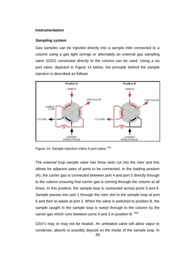
39

Instrumentation

Sampling system

Gas samples can be injected directly into a sample inlet connected to a

column using a gas tight syringe or alternately an external gas sampling

valve (GSV) connected directly to the column can be used. Using a six

port valve, depicted in Figure 14 below, the principle behind the sample

injection is described as follows.

Figure 14: Sample injection-Valco 6 port valve. (49)

The external loop sample valve has three slots cut into the rotor and this

allows for adjacent pairs of ports to be connected. In the loading position

(A), the carrier gas is connected between port 4 and port 5 directly through

to the column ensuring that carrier gas is running through the column at all

times. In this position, the sample loop is connected across ports 3 and 6.

Sample passes into port 1 through the rotor slot to the sample loop at port

6 and then to waste at port 2. When the valve is switched to position B, the

sample caught in the sample loop is swept through to the column by the

carrier gas which runs between ports 4 and 3 in position B. (43)

GSV’s may or may not be heated. An unheated valve will allow vapor to

condense, absorb or possibly deposit on the inside of the sample loop. In

40

the case where moist samples contain carbon dioxide for example, the

deposited layer of water may dissolve some of the carbon dioxide. Upon

injection of the sample, the gas will be flushed out of the loop quickly but

the carbon dioxide trapped in the water layer will be released slowly

causing the carbon dioxide peak to tail which in turn will affect any

quantitative measurements. Heating the GSV to 60°C or higher will

effectively remove this problem. The GSV may be heated by installing it in

the GC oven itself. (50) Alternatively a heating block, in which the valve can

be enclosed, can be purchased. The GC’s auxiliary temperature zone

controller is used to set and control the temperature. (50)

The sample loop should be flushed thoroughly with at least 100 ml of

sample prior to injection. If the sample quantity is limited, smaller flushing

volumes may be used provided there is sufficient sample to remove all of

the carrier gas or air previously contained in the loop. The alternative

solution to small sample volumes is to evacuate the sample loop and

associated gas lines. Vacuum and shut off valves should be installed as

close to the GSV as possible to keep the volumes as small as possible.

Samples injected at pressures below atmospheric create larger flow

disturbances than samples injected at higher pressures and it has been

noted that samples pressurized to the head pressure create almost no flow

disturbance. It must be noted that if a larger quantity of sample is injected,

the pressure must be known and this must be taken into account if the

pressure differs from that of the calibration standards. (50)

Pulsed discharge helium ionization detector

The advancement and versatility of gas chromatography as an analytical

tool has been largely based on improvements in sample introduction inlets,

column technology and detectors. There are two types of GC detectors,

those which respond to a wide range of chemicals and are termed

universal detectors and those which respond to a smaller range of

chemicals and are termed selective detectors. There is however a small

41

group of detectors which are capable of both universal and selective

modes of operation. These include the lesser known Pulsed Discharge

Detector (PDD). (51)

First described in 1992 (51), the PDD is based on an ionization source

resulting from a pulsed high voltage discharge between platinum

electrodes. When the discharge occurs in pure helium, a photon emission

results from the transition of diatomic helium to the dissociative 2He

ground state as indicated below.

He2 (A1∑u) → 2He (11S0) (22)

This transition is known as the Hopfield emission and occurs at very short

wavelengths (60 – 100 nm) with energies ranging from approximately 13.5

to 17.5 Ev. The broad emission provides sufficient energy to ionize all

elements and compounds excluding neon. The PDD can be configured as

a universal, selective or elemental detector. (51)

For universal detection, the GC column eluents are photoionized directly

by the Hopfield emission with the resulting electrons producing a

measured current. This type of configuration is referred to as the helium

pulsed discharge photoionization detector (He-PDPID). By adding small

amounts of an additional gas, called dopant, into the detector, selective

detection of electron capturing compounds can be achieved as the dopant

gas is ionized to establish a standing current. Electron capturing

compounds eluting from the GC lower this standing current. This

configuration is termed the pulsed discharge electron capture detector

(PDECD). Finally elemental detection is possible if the PDD is configured

with a monochromator and photomultiplier tube to measure the emission

lines which result from the analytes passing through the helium discharge.

This configuration is termed the pulsed discharge emission detector

(PDED). (51)

42

Figure 15: Cross section of the PDHID. (51)

The high voltage pulsed discharge is a simple ionization source. The

actual discharge occurs between two platinum electrodes which are

spaced approximately 2 mm apart. The platinum electrodes are made up

of a 0.25 – 0.05 mm diameter wire, tapered to points. The discharge

between the sharp platinum tips is fine with a thread like appearance and

the volume of the discharge region is small. The discharge is stable

resulting in a highly sensitive ionization detector. As the frequency of the

discharge is low and the intervals between the discharges are long, the

platinum electrodes are allowed to cool between pulses resulting in less

deterioration of the platinum electrodes over the long term. Since the

43

analyte signal presents an increase in ionization above that of the helium

carrier gas, stability of the discharge is absolutely critical. (6)

Compounds eluting from the column are ionized by high energy photons

originating from the helium discharge zone (Figure 15). Electrons

generated by this process are focused by the bias electrodes, towards the

collector electrode. The detector response arises as a result of changes in

the measured current. The separation of the discharge zone from the

ionization zone along with the counter helium gas flow configuration

ensures that only pure helium passes through the discharge region thus

minimizing the possibility of contamination of the discharge electrode. (51)

Ionization occurs by two processes. The first involves direct ionization of

the analyte by the electrons that have been accelerated by the high

voltage pulse:

e- (V) + He → He+ + 2e- (23)

In the second ionization process, ionization occurs by reaction of the

analyte with the relatively long-lived helium metastables. The helium

metastable state, 23S, is 19.7eV above the ground state and is capable of

ionizing any compound excluding neon which has an ionization potential of

21.5eV (6)

e- (V) + He → He** → He* (23S) + hv (24)

Factors affecting the detector signal include gas purity, temperature, flow

rate, pressure, chromatographic column and geometry of the cell. (52)

Using a permeation tube to create a range of moisture2.6.standards for calibration

Several methods have been developed for making up trace moisture

standards. The most absolute method involves saturating a gas stream

under known conditions. This method establishes an absolute reference

point. To create trace concentrations of moisture, cryogenic saturation

44

temperatures are needed and this method requires cumbersome

equipment which is not well suited for field applications. It is also limited to

gases which do not condense at the temperatures required to obtain very

low concentrations (53).

Because environmental moisture is so pervasive, there is no effective way

to predetermine the concentration of a final mixture. Part of this problem is

related to the storage of such a mixture. While it might be possible to add

a known quantity of moisture to a known volume of a gas matrix in a

container, the contribution of the container to the final concentration

cannot be determined. In addition the concentration may change over the

life of the mixture due to variations in temperature and pressure of the

contents. An additional uncertainty is introduced with the gas matrix which

may itself contain residual moisture and additional moisture may be

introduced in the process of transferring the matrix to the container. (53)

The permeation device is made up of a length of Teflon tubing into which

water has been sealed. Water vapor passes slowly through the tube wall

and into the surrounding atmosphere. By passing a flow of a clean, dry

gas over the tube (dilution gas), a known amount of moisture is added to

the gas flow. By keeping the tube at a constant temperature in a stream of

the dry gas for an extended period of time, and periodically weighing the

tube to measure the rate of weight loss, the rate of flow of moisture

emitted from the tube can be measured.(53) Figure 16 shows a diagram of

a basic permeation tube device.

The dilution flow and the permeating moisture combine to form a mixture.

This mixture now contains a known amount of moisture and the

concentration of this moisture is given by the following formula: (53)

C = (f / f + F) 106 (25)

Where:

C = concentration in ppm

45

f = permeation flow of moisture

F = flow of the dilution gas

Since the flow of moisture from the permeation tube itself is miniscule (nL

min-1) compared to the dilution flow from the dry gas (L min-1), the above

equation reduces to the following: (53)

C = (f / F) 106 (26)

The flow of moisture from the tube is described by the following equation:

F = k A Δp / t (27)

Where:

f = permeation flow

K = permeability of the membrane to water

A = surface area of the permeation

Δp = partial pressure difference of water across the membrane

t = thickness of the membrane

Figure 16: A basic permeation tube device (54)

46

The rate of addition of moisture to the gas stream can be set by selecting

permeation tubes that have different areas or thicknesses. It is also

possible to change the emission rate of a tube by changing the

temperature at which it permeates. There are two factors that affect the

temperature dependence of the permeation. The vapor pressure of water

varies as the temperature is varied and therefore Δp will vary exponentially

with inverse temperature. In addition, the permeability of the membrane

varies exponentially with inverse pressure. (53)

K = ko Exp (-B / T) (28)

Where:

Ko, B = equal constants

T = absolute temperature

The flow of moisture from a permeation tube is therefore strongly

dependent on the temperature of the tube and it is necessary to carefully

control temperature in order to make accurately known standard. (53) The

emission rate from a liquid fed permeation tube varies approximately 10%

per °C and a stable temperature is essential for attaining an accurate,

stable mixture. A system able to control the temperature to within ±0.1°C

will ensure emission accuracy within ± 1%. (55)

The flow path is provided by a fixed, continuous, uninterrupted carrier flow

over the permeation tube. A fixed carrier flow ensures that the component

concentration is constant and surfaces in the system equilibrate ensuring

rapid response while minimizing bias in the system. If a carrier flow is not

available, the permeation chamber and surrounding components are

quickly contaminated with a high concentration of the component

compound. (55)

Permeation tubes are useful in the preparation of very low concentration

standards. A tube emitting 50 nl min-1 of moisture mixed with a 1 l min-1

47

carrier flow generates a 50 ppbv mixture. If the carrier flow is changed to 5

l min-1, the same emission generates a 100 ppbv standard. Theoretically a

tube with an emission of 1 nl min-1, diluted in a 10 l min-1 carrier gas flow

should be able to generate a 100 pptv standard in a single dilution step but

there are practical limitations to be considered. With permeation tubes, the

basic limit is the minimum emission rate that can actually be measured.

Emission rates are determined by measuring the rate of weight loss. A

typical permeation tube weighs 10 to 15 g which is well within the range of

a semi micro balance. The minimum readable mass change is 0.01 mg

and a weight change of 1mg is needed to assure the possibility of

measuring weight loss at ±1% accuracy. For a 100 ng min-1 emission rate,

the smallest interval between weighing is 7 days. At 10 ng min-1, the

smallest interval is over two months thus making the minimum time for

emission certification approximately 8 months. (55)

An additional problem in the weighing process is that the Teflon

membrane develops a static charge which attracts any particles in the

sweep gas flowing over the tube during the emission measurement

process. The practical limit for a single stage dilution using a permeation

tube is 108:1. A solution to these problems is to use a secondary dilution

step for lower concentrations as indicated in Figure 17.

In this setup, a small portion of the primary mixture from the permeation

tube is split off and diluted into an additional flow of matrix gas. This

method can give 103: 1 to 105:1 additional dilutions meaning that a single

digit pptv mixture can be prepared with only 2 dilution stages and total

matrix gas consumption in the 2 - 10 l min-1 range. As concentrations

decrease, the purity of the gas matrix starts to have an effect. Unknown

background contamination may introduce large random errors. (55)

48

Figure 17: A typical permeation system flow (55)

49

CHAPTER 3: RESEARCH METHODOLOGY

Introduction3.1.

The methodology used in this research project, employed a combination of

analytical techniques for the measurement of the moisture content in

various gas samples. The techniques included GC/PDHID and FTIR. The

FTIR was initially set up as a control system as this is a known and

accepted method for moisture analyses, albeit for higher levels than were

attempted in this research. The FTIR was optimized initially for moisture

analyses using a moisture permeation reference standard and this was

followed by optimization for acetylene using a selection of acetylene

reference standards. Calibration curves were drawn up for both

components. The GC/PDHID was initially optimized and calibrated for both

moisture and acetylene analyses. A decision was taken not to risk the

PDHID filaments by directly injecting moisture into the system and hence

the system was only optimized and calibrated for acetylene. Following the

instrument setups, the conversion of moisture to acetylene was tested by

the addition of known amounts of moisture to excess amounts of calcium

carbide in 2 ml sealed vials. The experimental work involved adding known

amounts of moisture to the calcium carbide and injecting the gas formed

into the GC/PDHID. The GC/PDHID was initially used to test the

conversion process as the acetylene gas generated in this manner

produced volumes that were too small to analyze using the long path glass

gas cell which required at least 2000 ml of sample. Following these

experiments, a sample container was designed that fitted directly onto the

GC/PDHID and FTIR. The design of this sample holder was such that it

enabled the flow of a known amount of a gas, containing moisture, directly

into the sample container, allowed the reaction to occur and then by

addition of a carrier gas through the container, directly sweep the

acetylene formed into either the GC/PDHID or FTIR.

50

Section 1: FTIR experimental work3.2.

Commercial instrumentation

Bruker Tensor 27 Fourier Transform Infrared spectrophotometer with a

RockSolid, permanently aligned, high stability interferometer and spectral

range from 6000 to 500 cm-1 with “High Humidity” Zinc Selenide optics.

[Bruker Optik GmbH, Ettlingen, Germany]

Liquid nitrogen cooled MCT detector supplied by Bruker [Bruker Optik

GmbH, Ettlingen, Germany]

Bruker: Gas Cell 0.8 – 8 meters QL Gold mirror: P/N I10772.08, Type

A1366/3Q. Description: Variable path length 0.8 to 8 meters. External path

length control and cell volume approximately 2 liters. Glass cell body with

2 stainless steel valves for inlet and outlet as well as a safety valve.

Maximum pressure of 1.05 bars.

Low Volume Steel 2 m long path gas cell: Supplied by Axiom

Instrument control and data processing were done with a HP Compaq

personal computer (PC) utilizing the OPUS software, version 7.0, supplied

by Bruker. Bruker Optik GmbH, Ettlingen, Germany]

Consumables

Dessicant Cartridge for FTIR: Supplied by Bruker

Laser module: Supplied by Bruker

Gases

The following cylinder gases were obtained from Air Products South Africa

(Pty) Ltd. [Kempton Park, Gauteng]: Helium (5.0), Nitrogen (5.0) and

Synthetic air (4.0).

51

Note: The figures indicated in brackets behind the gas type are an

indication of the purity of that specific gas. For example, 5.0 indicates a

99.999% purity gas.

Liquid nitrogen was supplied by African Oxygen Limited (AFROX) [Alrode,

Gauteng]

Reference standards

Standard 1: Multicomponent Matheson reference standard 0.15% mixture

in nitrogen: Lot nr: 1059614693. Supplied by Puregas (Pty) LTD [Alrode,

South Africa]

Standard 2: Acetylene (100% by volume): Supplied by Air Products South

Africa (Pty) Ltd. [Kempton Park, Gauteng]

Standard 3: Acetylene (4835 ppm C2H2 in nitrogen): Certificate nr:

2258349: Supplied by Air Liquide South Africa Pty (Ltd) [Alrode, South

Africa]

Internal Standard: Methane 102 ppm in helium. Single component,

Matheson reference standard: Lot nr: 1023610432. Supplied by Puregas

(Pty) LTD [Alrode, South Africa]

Kintek Trace Source Disposable Permeation Tube, 159 ng min-1 at 30°C:

Lot nr: 47884. Supplied by Kintek [Strada Goretta, Caselle Torinese TO]

FTIR Instrument set up and optimization

General

The purpose of this section of the experimental work was to draw up a

calibration curve for moisture. From literature studies (9) and work done at

PAL it was deemed imperative to flush all the FTIR instrument

compartments with dry nitrogen to remove atmospheric moisture found to

be continuously present upon running scans on the evacuated glass cell.

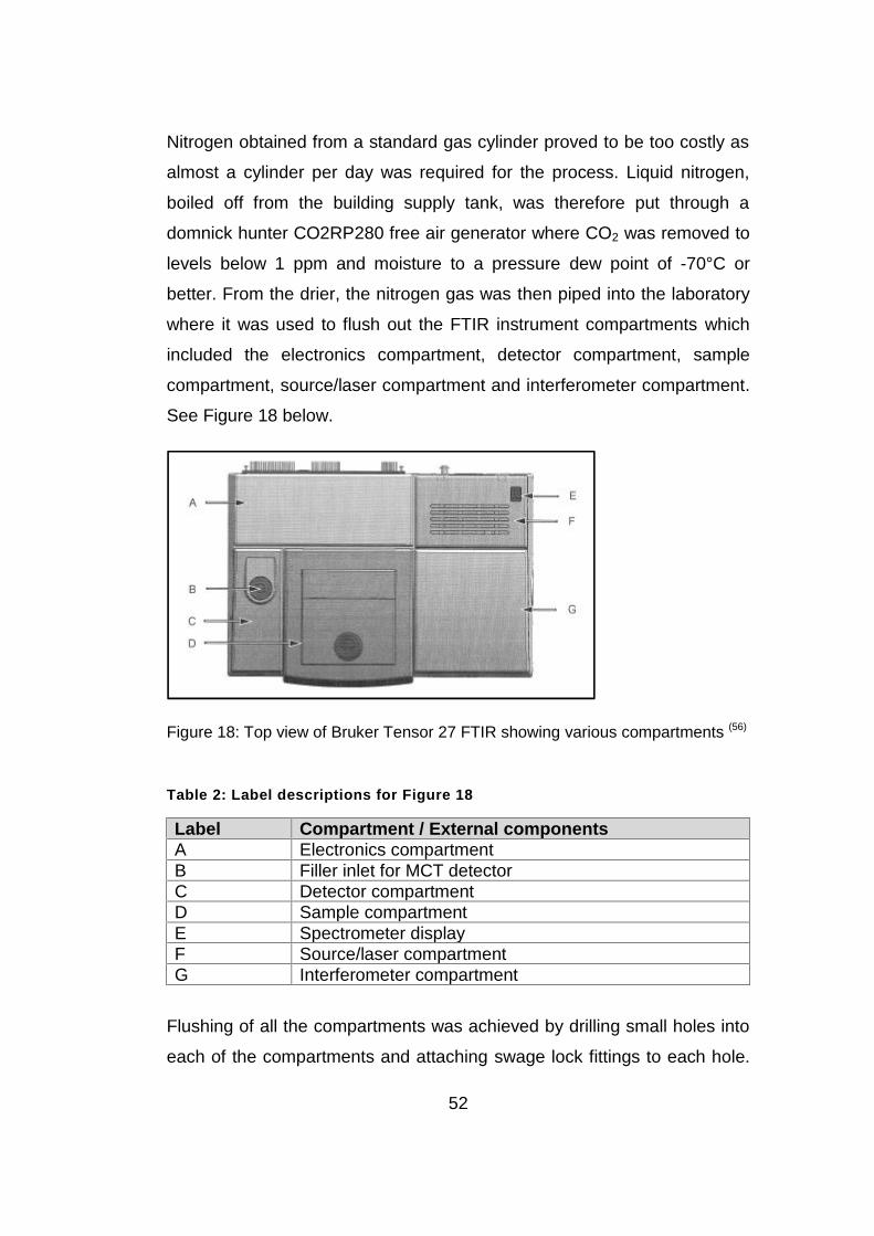
52

Nitrogen obtained from a standard gas cylinder proved to be too costly as

almost a cylinder per day was required for the process. Liquid nitrogen,

boiled off from the building supply tank, was therefore put through a

domnick hunter CO2RP280 free air generator where CO2 was removed to

levels below 1 ppm and moisture to a pressure dew point of -70°C or

better. From the drier, the nitrogen gas was then piped into the laboratory

where it was used to flush out the FTIR instrument compartments which

included the electronics compartment, detector compartment, sample

compartment, source/laser compartment and interferometer compartment.

See Figure 18 below.

Figure 18: Top view of Bruker Tensor 27 FTIR showing various compartments (56)

Table 2: Label descriptions for Figure 18

Label Compartment / External componentsA Electronics compartmentB Filler inlet for MCT detectorC Detector compartmentD Sample compartmentE Spectrometer displayF Source/laser compartmentG Interferometer compartment

Flushing of all the compartments was achieved by drilling small holes into

each of the compartments and attaching swage lock fittings to each hole.

53

These fittings were then connected to a central plastic pipe by which

nitrogen was flushed into each compartment. A rotameter was put in place

after the nitrogen inlet from the nitrogen tank and drier to ensure flow

control through the various compartments.

Detectors

The Bruker FTIR system was purchased by PAL in 2011. Both a DTGS

and MCT detector were included in the purchase. It was decided to use

the more sensitive MCT detector for the experimental work. The MCT

detector had to be filled with liquid nitrogen at the start of each day and

then replenished at least every three to four hours. It also required a

stabilization period of at least twenty minutes after each fill.

Gas cell

A variable long path, high volume glass gas cell, 0.8 m to 8.0 m (See

Figure 10) with calcium fluoride windows was used.

The recommended gas pressure range for the glass cell was 0 to 1 atm

and to ensure that the maximum pressure in the cell was never exceeded,

a pressure sensor and readout were connected to the outlet of the glass

cell. In addition, a back pressure regulator was added to the glass cell exit,

enabling control of flow and pressure through the glass cell at all times.

At the inlet of the gas cell, a three way valve was connected. This allowed

for a vacuum with which to evacuate the cell or upon rotation of the valve

handle, nitrogen could be selected to flush the cell or standards/samples

could be sent through to the glass cell for analyses. See Figure 19 for

instrument set up.

54

Figure 19: Schematic of FTIR set up for experimental work

Moisture is a highly pervasive component of air, and had to be thoroughly

removed from the glass cell before any analyses could be performed.

Despite drawing a vacuum on the cell over two days and attempting to

flush out the cell with both nitrogen and then helium for a similar period,

moisture was still present and could be clearly seen upon running a scan.

Heating tape was then wrapped around both the glass cell as well as all

the steel pipe lines running through to the glass cell (9). A controller with

which to control the temperature was designed and installed in order to

prevent the glass cell from overheating. Initial tests were run keeping the

glass cell at 50°C.

55

As it appeared from early experimental work that the glass cell retained a

certain amount of moisture despite heating and flushing processes

implemented, a second single pass, folded Axiom steel gas cell was set up

in exactly the same manner as the glass cell. It was expected that the

concentration range obtained using the low volume steel cell would be

higher than that obtained for the glass cell due to the shorter path length of

the low volume cell. The advantage of the low volume cell was that it could

be heated at much higher temperatures than the glass cell and also

required much less sample due to its smaller internal volume.

Unfortunately upon setting up this low volume cell, it was found that it

could not be sufficiently sealed, due to its design, from atmospheric

moisture ingress and thus could not be tested for this project.

Background

A background was drawn using the same nitrogen used for dilutions of the

moisture permeation standard. The purpose of the background is to detect

the influence of the ambient conditions i.e. air humidity, temperature and

the spectrometer itself on the spectroscopic measurement results. OPUS

automatically calculates the results sample spectrum by dividing the

sample spectrum by the background spectrum. This ensures that the

spectral bands resulting from ambient conditions and from the

spectrophotometer are eliminated from the sample spectrum. (56)

Dilution system

In order to obtain a range of standards for both the moisture and acetylene

calibration curves, the initial reference standards had to be diluted down to

the desired concentration levels. A dilution system, designed and built at

PAL, was available from a previous project. The system has four

Bronkhorst High Tech mass flow controllers (MFC) in the following ranges:

0 – 50 ml min-1

0 – 100 ml min-1

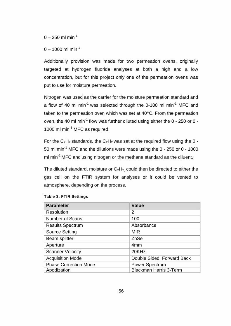
56

0 – 250 ml min-1

0 – 1000 ml min-1

Additionally provision was made for two permeation ovens, originally

targeted at hydrogen fluoride analyses at both a high and a low

concentration, but for this project only one of the permeation ovens was

put to use for moisture permeation.

Nitrogen was used as the carrier for the moisture permeation standard and

a flow of 40 ml min-1 was selected through the 0-100 ml min-1 MFC and

taken to the permeation oven which was set at 40°C. From the permeation

oven, the 40 ml min-1 flow was further diluted using either the 0 - 250 or 0 -

1000 ml min-1 MFC as required.

For the C2H2 standards, the C2H2 was set at the required flow using the 0 -

50 ml min-1 MFC and the dilutions were made using the 0 - 250 or 0 - 1000

ml min-1 MFC and using nitrogen or the methane standard as the diluent.

The diluted standard, moisture or C2H2, could then be directed to either the

gas cell on the FTIR system for analyses or it could be vented to

atmosphere, depending on the process.

Table 3: FTIR Settings

Parameter ValueResolution 2Number of Scans 100Results Spectrum AbsorbanceSource Setting MIRBeam splitter ZnSeAperture 4mmScanner Velocity 20KHzAcquisition Mode Double Sided, Forward BackPhase Correction Mode Power SpectrumApodization Blackman Harris 3-Term

57

Method 1: H2O analysis on FTIR3.3.

General

The purpose of this section of the experimental work was to draw up a

calibration curve for moisture using a permeation standard.

Variation of gases used for dilutions

At the start of the experimental work, various gases were tested as both

diluents for the permeation standard and for flushing the FTIR

compartments. These included both helium and argon as both were found

to contain less moisture than the nitrogen boiled of from the building

supply. Due to the expensive nature of these two gases, it was decided to

return to the original choice and to compensate for any additional moisture

by heating the glass cell.

Optimizing the glass gas cell temperature

In order to determine the optimum temperature at which to run the glass

cell for moisture analyses, a moisture calibration curve was initially drawn

up at 50°C using the permeation standard, to obtain a rough estimate of

the moisture content of the glass cell. The cell temperature was then

systematically increased by 10°C from 40°C up to 110°C while flushing

continuously with nitrogen and five moisture readings taken at every

temperature change. The cell was allowed to stabilize at each temperature

for at least 4 hours. The moisture results obtained in ppmv were plotted

against the temperature changes as indicated in Figure 20. Based on

these results, it was decided to recalibrate the FTIR for moisture keeping

the cell temperature and stainless steel lines at a temperature of 40°C.

58

Figure 20: Plot of H2O concentration versus cell temperature for glass cell

Moisture permeation reference standard: KINTEK

A Kintek Trace Source Disposable Moisture Permeation Tube, with an

emission rate of 159 ng min-1 at 30°C, was selected as a reference

standard. The disposable permeation tube was placed in a steel holder

designed with an inlet for the nitrogen carrier gas and an outlet for the

diluted moisture mixture (see Figure 21). This steel holder was sealed and

inserted into a permeation oven designed and built at PAL. The

permeation oven was set to 40°C and a flow of 40 ml min-1 of nitrogen,

controlled by a mass flow controller with a range of 0 to 50ml min-1, was

used to carry the moisture permeation standard through to the FTIR gas

cell. The permeation rate of 159 ng min-1 is based on a temperature of

30°C as per the certificate of analysis (See Appendix 1) but due to the

permeation oven design; the lowest temperature that could be set was

40°C. A The following calculation was used to calculate the rate change

with temperature change (57)

Log P1 = Log P0 + α (T1 – T0) (29)

Where:

0

0.005

0.01

0.015

0.02

0.025

0 20 40 60 80 100 120 140

H2O

con

cent

ratio

n (p

pm)

Temperature °C

Varying the glass cell temperature

59

P0 = Rate at temperature T0 (°C)

P1 = New rate at temperature T1 (°C)

α = the temperature coefficient (0.034 for standard emission tubes)

Using above calculation, where the emission rate (159 ng min-1 at 30°C) is

calculated at 40 °C, is as follows:

Log P1 = Log 159 + 0.034 (40 – 30) = 318 ng min-1

Figure 21: Typical permeation tube and permeation tube holder (58)

60

In order to draw up a calibration curve, the initial moisture mixture flowing

from the permeation holder had to be further diluted to obtain a range of

concentrations. This was achieved by adding additional volumes of

nitrogen, regulated by mass flow controllers, to the flow of permeation

standard flowing from the permeation holder and oven. A gas dilution

system, designed and built in-house, was used to dilute the initial moisture

permeation standard down to 8 different levels from which a calibration

curve could be drawn up. The moisture, permeating at a fixed rate of 318

ng min-1 (see equation 29), from the permeation tube sealed inside the

permeation oven, was carried from the permeation oven to the FTIR using

a Bronkhorst mass flow controller with a range of 0 to 50 ml min-1 as

indicated in the section above. This flow of 40 ml min-1 was kept constant.

The nitrogen diluent flow was controlled by an additional two Bronkhorst

mass flow controllers, one ranging from 0 to 250 ml min-1 and one ranging

from 0 to 5000 ml min-1. The diluent was added to the 40 ml min-1

permeation flow prior to reaching the long path glass gas cell. Mixing of

the diluent and standard took place in the dilution system and the resultant

gas mixture was loaded directly from the dilution system into the long path

gas cell at a 100 kPa. Table 4 summarizes the diluent and standard flows

used to obtain a range of calibration levels from the moisture permeation

standard at 318 ng min-1.

Table 4: Dilution of moisture permeation standard to obtain calibration levels

Diluent flow(ml min-1)

Permeation flow(ml min-1)

Total Flow(ml min-1)

[ H2O] (ppmv)

730 40 770 0.514460 40 500 0.791305 40 345 1.147160 40 200 1.978110 40 150 2.63760 40 100 3.9560 40 40 9.890

61

Calculations to obtain ppmv values from dilutions

The calculations performed to acquire the emission rate as ppmv after

dilution was done as follows:

ppmv = K0 x ng min-1 / F

Where:

K0 is the equal constant (from the suppliers COA)

ng min-1 is the permeation rate (calculated at 40°C: See equation 29) and

F is the total dilution flow in ml min-1 and includes permeation flow and

dilution gas flow in ml min-1

Peak selection

Moisture typically has two spectral ranges in which peaks can be selected

for quantitation namely 3890 to 3560 cm-1 and 1840 to 1410 cm-1. A total

of eleven different peaks in both ranges were selected for quantitation, as

indicated in Figure 22 below.

Figure 22: Typical FTIR spectra of H2O indicating peaks selected for quantitation C:\OPUS_7.0.129\MEAS\29072014\Std 0.978ppm 40_100ml_min.0 Std 0.978ppm 40_100ml_min Background on BN2 2014/07/30

3853.9635

3712.4381

3688.7629

1734.4073

1685.0288

1652.9327

1635.6503

1617.5448

1576.3960

1539.3621

1456.2416

100015002000250030003500Wavenumber cm-1

0.00

00.

001

0.00

20.

003

0.00

40.

005

0.00

6Ab

sorb

ance

Uni

ts

Page 1/1

62

The purpose of this selection was to determine which of the eleven peaks

were most suited, statistically, for use. The large peak between 3000 and

3500 cm-1, on all the H2O graphs that follow, could not be identified and

was subsequently not identified / labelled on the spectra.

Calibration for moisture

At the start of the project, a moisture calibration curve was drawn up with a

concentration range from 0.404 ppmv to 9.890 ppmv moisture using the

peak at wavenumber 3854 cm-1 (see Table 4) and the glass cell and

stainless steel lines heated to and kept at 50°C. This calibration curve,

although not optimum, was used to get rough values to determine the

optimum cell temperature to use for the glass cell.

After stabilizing the glass gas cell at the selected temperature of 40°C,

new calibration curves were drawn up at each of the previously selected

wavenumbers and using the same dilution standards as discussed

previously. The lowest calibration standard was run first and after each

change in flow rate to obtain the next calibration level, 4 hours was

allowed for stabilization of dilution flows and equilibration of the cell.

Eleven different calibration curves were obtained, one for each selected

wavenumber (see Appendix 2). Both linear and quadratic fits were applied

to the calibration data and the results compared.

Use of methane to prove stability of FTIR system

From the calibration curve obtained for moisture in the previous

experiment, it was clear that there was a wide spread of results around

each calibration point specifically around the highest calibration level. This

indicated instability in the moisture readings at each level, possibly due to

adsorption of moisture on the glass cell walls or perhaps a problem with

the instrument itself. In order to determine if this was a problem created by

the instrument/cell or if it was only present for the moisture analysis,

methane was selected as an additional component for FTIR analysis, a

63

reference standard being readily available in the laboratory. The following

spectrum was obtained for methane at 3018 cm-1:

Figure 23: Typical FTIR spectra of CH4 indicating peak selected for quantitation

Table 5 summarizes the diluent and standard flows used to obtain a range

of calibration levels from the 9.93 ppmv CH4 reference standard.

Table 5: Dilution of CH4 reference standard to obtain calibration levels


CH4 flow(ml min-1)


[CH4] (ppmv)

2460 50 2510 0.1982460 100 2560 0.3881760 100 1860 0.534960 100 1060 0.937460 100 560 1.773305 100 405 2.452110 100 210 4.729

Visually the spread of results around each calibration point appeared to be

smaller than that obtained for the moisture tests, indicating that the

problem with the spread of results around the moisture calibration levels

64

was related to the moisture and possible adsorption to the glass walls of

the cell and not the instrument.

CH4 as internal standard for moisture analyses

In order to compensate for the spread of the results around each

calibration point, it was decided to attempt to use methane as an internal

standard for the moisture analyses in order to compensate/correct for loss

of the analyte (moisture) during sample inlet. Calibration was obtained by

plotting the ratio of the moisture signal to the CH4 signal as a function of

the analyte concentration of the standards. The CH4 was initially tested for

stability by using it to draw up a calibration curve in the same manner as

was done for the moisture and by visually examining the spread of results

around each calibration point.

Method 2: C2H2 analysis on FTIR3.4.

General

The purpose of this second section of the experimental work was to draw

up a calibration curve for C2H2 using FTIR. The instrument set-up was

identical to the set-up for experiment 1, the only difference being that the

glass cell was not heated for the C2H2 experimental work.

Background

A background was run using the same nitrogen used for dilutions of the

C2H2 standard dilutions.

Summary of acetylene reference standards tested:

Initially the certified 0.15% Matheson reference standard (Standard 1)

containing 27 different components, including C2H2, was used to set up a

calibration curve on the FTIR. Taking a spectrum from literature, four

peaks were identified for quantitation purposes namely, a combination of

3313 / 3266 cm-1 as well as 1350 cm-1 and 1305 cm-1. Problems were

detected using Standard 1.

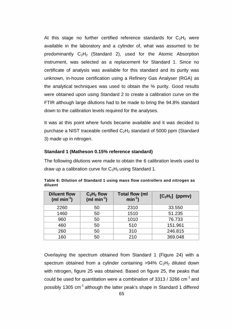
65

At this stage no further certified reference standards for C2H2 were

available in the laboratory and a cylinder of, what was assumed to be

predominantly C2H2 (Standard 2), used for the Atomic Absorption

instrument, was selected as a replacement for Standard 1. Since no

certificate of analysis was available for this standard and its purity was

unknown, in-house certification using a Refinery Gas Analyser (RGA) as

the analytical techniques was used to obtain the % purity. Good results

were obtained upon using Standard 2 to create a calibration curve on the

FTIR although large dilutions had to be made to bring the 94.8% standard

down to the calibration levels required for the analyses.

It was at this point where funds became available and it was decided to

purchase a NIST traceable certified C2H2 standard of 5000 ppm (Standard

3) made up in nitrogen.

Standard 1 (Matheson 0.15% reference standard)

The following dilutions were made to obtain the 6 calibration levels used to

draw up a calibration curve for C2H2 using Standard 1:

Table 6: Dilution of Standard 1 using mass flow controllers and nitrogen asdiluent


C2H2 flow(ml min-1)

Total flow (mlmin-1)

[C2H2] (ppmv)

2260 50 2310 33.5501460 50 1510 51.235960 50 1010 76.733460 50 510 151.961260 50 310 246.815160 50 210 369.048

Overlaying the spectrum obtained from Standard 1 (Figure 24) with a

spectrum obtained from a cylinder containing >94% C2H2 diluted down

with nitrogen, figure 25 was obtained. Based on figure 25, the peaks that

could be used for quantitation were a combination of 3313 / 3266 cm-1 and

possibly 1305 cm-1 although the latter peak’s shape in Standard 1 differed

66

from that in the >94% C2H2 indicating some form of interference from one

of the other components in standard 1. The peak at 1350 cm-1 appeared

to be non-existent in Standard 1 and was therefore omitted from the

calibration setup.

Figure 24: Spectrum obtained for Standard 1

Figure 25: Overlay of Standard 1 with a >94% C2H2 standard. The insert shows aclose up of the peaks at 1350 and 1305 cm-1.

67

Standard 2 (C2H2 standard certified in-house)

The in-house C2H2 was certified using RGA and the concentration was

determined to be 94.8%. Since this concentration was too high to be

diluted directly down to the required calibration levels using the mass flow

controllers available, as was done for the Matheson standard, a second

dilution system was brought in. Standard 2 was put through the first

dilution system and diluted down to 9384 ppm using a standard flow of 10

ml min1- and a nitrogen diluent flow of 1000 ml min1.

The following dilutions were then made from the 9384 ppm diluted

standard to obtain the 7 calibration levels used to draw up a calibration

curve for Standard 2:



C2H2 Flow(ml min-1)


[C2H2] (ppmv)

2500 40 2540 147.781500 40 1540 243.741000 40 1040 360.93800 40 840 446.87450 40 490 766.05250 40 290 1294.37100 40 140 2681.19

Figure 26 shows the spectrum obtained for Standard 2. From this

spectrum it appeared that the 4 peaks originally selected, 3313 / 3266 cm-1

as well as 1350 cm-1 and 1305 cm-1 were available for quantitation.

68


Standard 2 with internal standard

For this experimental work, CH4 was added as an internal standard to

Standard 2. A CH4 reference standard of concentration 9.9 ppm, balance

of nitrogen, was used as the diluent in place of the nitrogen previously

used. The following dilutions were made to obtain the 7 calibration levels

used to draw up a calibration curve for Standard 2 with CH4 as internal

standard:

Table 8: Dilutions of Standard 2 using mass flow controllers and 9.9 ppmCH4 standard in nitrogen as diluent

CH4 diluent flow(ml min-1)

C2H2 flow(ml min-1)

Total flow(ml min-1)

[C2H2](ppmv)

[CH4](ppmv)

2500 50 2550 184.00 9.711500 50 1550 302.71 9.58800 30 830 339.19 9.54

1000 40 1040 360.93 9.52450 20 470 399.33 9.48450 20 490 507.25 9.36390 25 415 565.31 9.32

69

Figure 27: Spectrum obtained on analysing Standard 2 using CH4 as internalstandard at 3017 cm-1.

Standard 3 (Air Liquide C2H2 reference standard)

The following dilutions were made to obtain the 7 calibration levels used to

draw up a calibration curve for C2H2 using Standard 3:



C2H2 flow(ml min-1)


[C2H2] (ppmv)

2500 50 2550 94.8041500 50 1550 155.9681000 40 1040 185.962450 20 470 205.745800 40 840 230.238350 20 370 261.351390 25 415 291.265

G:\MSC 2014\Experimental\13112014\MEAS\07102014\07102014_Std 5 CH4_450 and C2H2_20_421.319ppm.8 07102014_Std 5 CH4_450 and C2H2_20_421.319ppm Actual standard2014/10/07

3314.21453265.8250

3017.4256

1349.60101307.6635

100015002000250030003500Wavenumber cm-1

0.00

00.

005

0.01

00.

015

0.02

00.

025

0.03

0Ab

sorb

ance

Uni

ts

Page 1/1

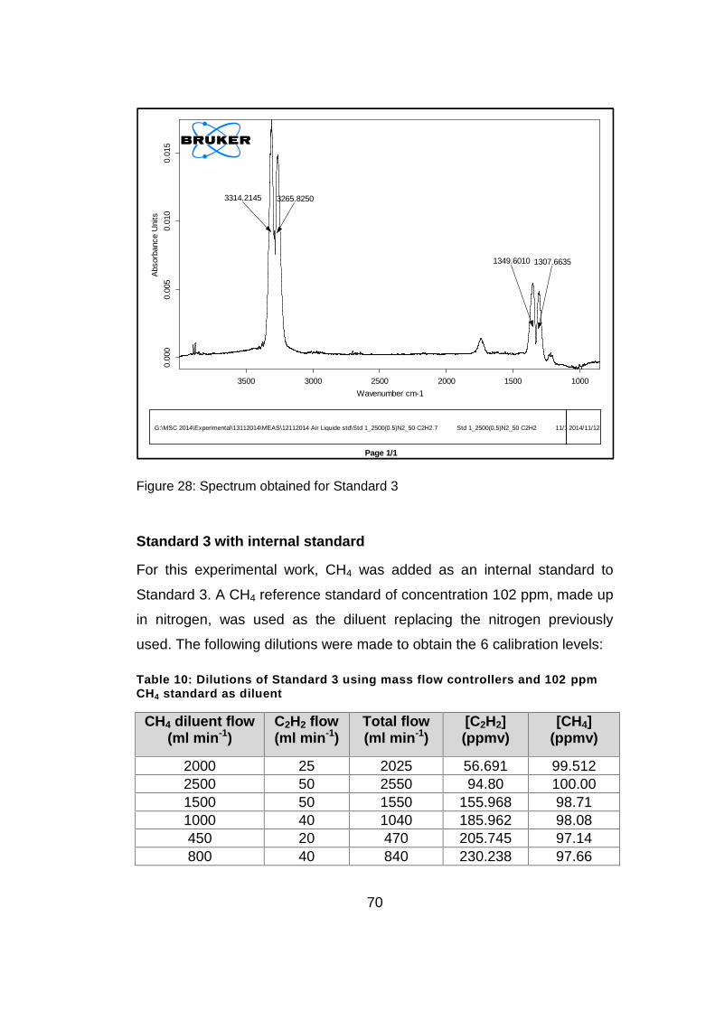
70


Standard 3 with internal standard

For this experimental work, CH4 was added as an internal standard to

Standard 3. A CH4 reference standard of concentration 102 ppm, made up

in nitrogen, was used as the diluent replacing the nitrogen previously

used. The following dilutions were made to obtain the 6 calibration levels:

Table 10: Dilutions of Standard 3 using mass flow controllers and 102 ppmCH4 standard as diluent

CH4 diluent flow(ml min-1)

C2H2 flow(ml min-1)


[C2H2](ppmv)

[CH4](ppmv)

2000 25 2025 56.691 99.5122500 50 2550 94.80 100.001500 50 1550 155.968 98.711000 40 1040 185.962 98.08450 20 470 205.745 97.14800 40 840 230.238 97.66

G:\MSC 2014\Experimental\13112014\MEAS\12112014 Air Liquide std\Std 1_2500(0.5)N2_50 C2H2.7 Std 1_2500(0.5)N2_50 C2H2 11/12/14 12:30:502014/11/12

3314.2145 3265.8250

1349.6010 1307.6635

100015002000250030003500Wavenumber cm-1

0.00

00.

005

0.01

00.

015

Abso

rban

ce U

nits

Page 1/1

71

G:\MSC 2014\Experimental\13112014\MEAS\07102014\07102014_Std 5 CH4_450 and C2H2_20_421.319ppm.8 07102014_Std 5 CH4_450 and C2H2_20_421.319ppm Actual standard2014/10/07

3314.2145

3265.8250

3017.4256

1349.60101307.6635

100015002000250030003500Wavenumber cm-1

0.00

00.

005

0.01

00.

015

0.02

00.

025

0.03

0Ab

sorb

ance

Unit

s

Page 1/1

Figure 29: Spectrum obtained on analysing Standard 3 with CH4 as internalstandard at 3017 cm-1.

Section 2: GC experimental work3.5.

Commercial instrumentation

Agilent 7890 Gas Chromatograph [Agilent Technologies, 5301 Stevens

Creek Blvd, Santa Clara, CA, USA] equipped with a Valco 6 port valve and

a VICI D-3 Pulsed Discharge Helium Ionization detector. [Valco

Instruments Company Inc. Schenkon, Switzerland].

Agilent Software: OpenLAB CDS, Chemstation Edition, Rev. C. 01.03 (37)

Consumables

Haysep Q Silcosteel packed column: Mesh 80/100, ID 2.1 mm and length

5 m. Maximum temperature of 275°C.

Haysep N Nickel packed column: Mesh 80/100, ID 2.1 mm and length 4 m.

Maximum temperature of 165°C.

72

Gases

The following cylinder gases were obtained from Air Products South Africa

(Pty) Ltd. [Kempton Park, Gauteng]: Helium (5.0), Nitrogen (5.0) and

Synthetic air (4.0).

Reference standards

Multicomponent Matheson reference standard 0.15% mixture in nitrogen:

Lot nr: 1059614693. Supplied by Puregas (Pty) LTD [Alrode, South Africa]

GC/PDHID set up and optimization3.6.

General

The performance of a PDHID detector is adversely affected by the

presence of any impurities in the carrier or discharge gas streams. The GC

system was therefore set up using helium (5.0) as carrier gas. The helium

was connected directly to the GC, unlike the other instruments in the

laboratory where a central source of helium is used for all the systems in

the laboratory. The purpose of this was to keep air ingress to a minimum

by limiting the length of the helium flow path. In addition the helium was

put through heated purifiers to ensure the removal of water vapor and any

fixed gas impurities that could be present. The purified helium was then

split between the detectors and the columns using an electronic flow

control device.

Valve configuration

The GC/PDHID was initially set by Scientific Supply Services cc who were

contracted by Chemetrix upon PAL’s purchase of the 7890 GC in 2011.

Two six port Vici valves were installed together with two Vici PDHID’s. The

detectors and valves were set up as two independent systems with the

possibility of linking them in future, depending on the type of analyses

required. A sample inlet was designed in-house and linked to the GC. The

sample inlet included a point whereby vacuum could be drawn to evacuate

73

the sample lines, a two way valve which could be switched between

sample and calibration standards as required and a point connected to a

helium source which could be used to flush the inlet with helium if

required.

The system was initially setup such that in position A, the sample loop is

filled and when the valve switches to position B, the contents of the loop

are injected onto the column. This configuration is referred to as “Sample

Injection”. See Figure 30 below.

Figure 30: In position A on the left, the sample loop is filled and in position B onthe right, the contents of the loop are injected onto the column. (59)

Subsequent to this setup, problems were encountered after injection of the

first reference standard. Due to financial constraints at NECSA, no funds

were available for the purchase of a single component acetylene reference

standard and it was decided to use the available twenty seven component

mix, one of the components being 0.155% C2H2. Acetylene elutes at

approximately six minutes but the runtime had to be extended to thirty

minutes in order to elute the remaining components. It was also found that

the mixture of organic components caused the PDHID baseline to increase

and additional time was required to stabilize the baseline after each run.

74

In a commercial laboratory, time is money and the quicker a sample can

be analyzed, the greater the number of sample that can be run in a given

period hence it was decided to re-plumb the system from a “Sample

injection” configuration to a “Loop sampling with backflush of pre-column

to vent” configuration. The “Loop sampling with backflush of pre-column to

vent” plumbing scheme allows “heavy” eluting components with long

retention times to be back flushed to waste. After the sample loop is

loaded in position A, the valve is switched to position B to inject the

sample onto column 1. Once all the components of interest have entered

column 2, the valve is switched back to position A and column 1 is

backflushed to vent during the analysis, reducing the total analysis time.(60) The “Loop sampling with backflush of pre-column to Vent” plumbing

scheme is indicated in figure 31 below.

Figure 31: In position A on the left, the sample loop is loaded/column 1 isbackflushed and in position B on the right, the sample is sent to the columns (60)

Above configuration led to a modicum of success as all organic

components eluting after the acetylene could be backflushed. However,

the long term goal of the project is the analysis of high purity permanent

gases such as nitrogen and oxygen in the 99, 9999% range. Since most of

the permanent gases will elute prior to the acetylene and in much larger

quantities than the acetylene, a massive disturbance in the PDHID

baseline will be observed. In order to combat this problem, the major

75

component of the permanent gas being analysed must be eliminated from

the analytical column before reaching the detector.

To address this problem, a valve configuration termed the “Sample

injection and heart cut to detector” was setup. In this configuration the

sample loop is loaded in position A. When the valve switches to position B,

the loop contents are injected onto the analytical column and the front cut

(containing the major permanent gas component being analysed) is eluted

from the column and goes to vent. At this point the valve is switched back

to position A, and the heart cut section containing the acetylene is

backflushed to the detector. Once the acetylene has eluted, the valve is

switched back to position B, sending the end cut to vent. (61) See Figure 32

below for the “Sample injection and heart cut to detector” configuration.

Figure 32: In position A on the left, the sample loop is loaded in the initial stepand in the second step the heart cut is sent to the detector. In position B on theright, the loop contents are sent to the column in the initial step and in the secondstep the end cut is sent to waste. (61)

According to Hayes Separations, INC (62), the Haysep Q or HayesepT

packed column would provide adequate analyses of acetylene. A Hayesep

Q, five metre, 80/100 mesh was selected as the analytical column and a

four meter Hayesep N, 80/100 mesh was selected as the pre-column.

76

The GC was configured such that a flow of thirty ml/min of Helium passed

through the discharge region of the PDHID and a flow of twenty ml min-1

through the column. The detector was kept at a temperature of 150°C.

Grade 5 helium (99.999%) was used at all times and it was additionally

purified using a VICI helium purifier, prior to entering the PDHID and the

analytical column. The valve box was heated to 60°C and the column

temperature was isothermal at 80°C throughout each run.

GC/PDHID experimental work3.7.

General

The purpose of this second section of the experimental work was to draw

up a calibration curve for acetylene using the GC/PDHID and then analyze

samples containing moisture and in which the moisture had been

converted to C2H2 via reaction with calcium carbide.

Dilution of standards using mass flow controllers

A dilution system, designed and built in-house, was used to dilute the

original 0.15% Matheson reference standard down to eight different levels

from which a calibration curve could be drawn up. The nitrogen diluent

flow was controlled by a mass flow controller with a range of 2500 to 50 ml

min-1 and the reference standard was controlled by a mass flow controller

with a range of 1 to 20 ml min-1. Mixing of the diluent and standard took

place within the dilution system and the resultant gas mixture was loaded

directly from the dilution system into the sample loop on the GC at a 100

kPa. Table 11 below summarizes the diluent and standard flows used to

obtain a range of calibration levels.

77

Table 11: Dilution of C2H2 standard using mass flow controllers


Standard flow(ml min-1)

[C2H2] (ppmv)

2500 1.0 0.6201800 1.0 0.8611500 1.0 1.0331000 1.0 1.584800 1.0 1.935600 1.0 2.579400 1.0 3.865300 1.0 5.150250 1.0 6.175200 1.0 7.711

Calculations to obtain ppmv values for dilutions

The calculations performed to acquire the concentration of C2H2 as ppmv

after dilution was done as follows:

ppmv = Fs / (Fs + FD) x CS

Where:

Fs = Flow of Reference standard in ml min-1

FD = Flow of Diluent gas in ml min-1

CS = Concentration of Reference standard in ppmv

Section 3: Conversion of moisture to C2H23.8.

Consumables

Calcium Carbide (100g/0.3-1 mm): Supplied by Fluka: Purity >75%: Lot nr-

437549/1

Agilent Technologies 2ml clear wide opening glass crimp cap vial: Lot nr-

924-01-13/001: Supplied by Chemetrix

78

1µl SGE Type B Plunger needle syringe P/N:020705: Supplied by SGE

Optimization of the conversion process using vials

GC/PDHID was initially selected as the analytical method for the

optimization of the conversion process primarily due to the low sample

volumes generated in the initial testing processes. Conversion of moisture

to C2H2 was initially undertaken in 2ml GC vials which were tightly sealed

using crimp caps and a capper. The initial tests included the following:

CaC2 was added to 5 vials and the vials sealed. The headspace from

each vial was analyzed using the headspace above the CaC2.

CaC2 was added to 5 vials and the vials then purged with a light flow of

helium for 5minutes. The vials were then sealed and the headspace

from each vial was analyzed using the headspace above the CaC2.


helium for 5 minutes. The vials were then sealed. 1 µl of H2O (l) was

added to each vial, using a 1 ul syringe and inserting the liquid via the

cap septum. The headspace of each vial was analyzed.


helium for 5 minutes. The vials were then sealed. Each vial was tared

using a 5 decimal place balance and 1 µl of H2O (l) was added to each

vial, using a 1 ul syringe and inserting the liquid via the cap septum.

The mass of H2O (l) added was recorded. The headspace of each vial

was analyzed.

Sample holder for conversion process

The crimp cap vials worked well for the optimization of the conversion

process using H2O (l) but a bigger container was required for gas sampling.

A sample holder was put together using Swagelok fittings (See Figure 33).

A digital pressure gauge was connected to the holder and provision was

made to either evacuate, or fill the holder with helium as required. The

central compartment was filled with CaC2, contained on either side by

79

glass wool. An inlet, sealed with a rubber septum, directly coupled to the

CaC2 in the holder was used to add moisture for the conversion reaction

using H2O (l). Alternately a quantity of gas sample, containing H2O could be

loaded into the holder, and once the reaction had occurred, the liberated

acetylene could be swept through to the GC or FTIR using the helium inlet.

Figure 33: Sample holder for CaC2/H2O reaction

The sample holder was initially flushed with helium to remove any

atmospheric moisture which reacts with the calcium carbide giving higher

results than expected. A known mass of water was added to the

evacuated sample holder containing the calcium carbide. The holder was

pressurized to 100 kPa with helium and allowed to stand for 2 to 3

minutes. Thereafter aliquots were transferred from the holder to the GC or

FTIR and the acetylene concentrations (ppmv) calculated back to moisture

values. An initial run with high % recovery indicated air ingress and the

holder was then sealed and purged externally with helium. Results

obtained for both GC and FTIR are discussed in Chapter 4.

80

CHAPTER 4: RESULTS AND DISCUSSION

Method 1: H2O analysis on FTIR4.1.

Optimization of the glass cell temperature

From the plot of H2O concentration versus cell temperature for the glass

cell in Figure 20, it can be seen that an increase in the moisture

concentration occurred as the temperature of the glass cell was

systematically raised from 40°C to 120°C. The supplier of this particular

glass cell indicated that the cell could be heated to 200°C using a standard

heating mantle designed specifically for the cell. Unfortunately this was not

available at PAL and an in-house system, utilizing heating tape and a

sensor, was set up as an alternative to the heating mantle. It was decided

not to increase the temperature beyond 120°C during the testing as there

was a concern that the glass cell electronics risked overheating and

possible damage. From the plot of H2O concentration versus cell

temperature for glass cell, 40°C was selected as the optimal temperature

for the moisture analysis. No temperature optimization was done for the

C2H2 tests as stabilization at different calibration levels was rapidly

reached, unlike for the moisture tests where hours of stabilization was

required between each level.

Calibration results for moisture

Calibration data was generated as per section 3.3. A typical linear

calibration curve for wavenumber 3854 cm-1, obtained from Excel, is

shown in figure 34 below. All calculated parameters for the calibration

curves at the selected wavelengths are indicated in Tables 12 through to

16 below. The concentration ranges are classified as follows: Level 1:0.514 ppm to 9.890 ppm and Level 2: 0.514 to 3.956 ppm

81

y = 0.0002x + 8E-06R² = 0.97

-0.0005

0

0.0005

0.001

0.0015

0.002

0.0025

0 2 4 6 8 10 12

Resp

onse

Fac

tors

Concentration (ppm)

Linear Calibration curve for H2O at 3854 cm-1:0.514 to 9.890 ppm

Figure 34: Linear calibration curve for moisture at 3854 cm-1 with a working rangebetween 0.514 and 9.890 ppm

Table 12: Summary of linear regression data for moisture standard:Confidence intervals for the intercept.

Wavenumber (cm-1) Range (ppm) Lower 95% Upper 95%3854 Level 1 -8.14938E-06 2.28403E-05

Level 2 -4.87399E-05 -2.13524E-053712 Level 1 2.65291E-05 6.41903E-05

Level 2 -3.03179E-05 -4.81437E-063689 Level 1 5.83273E-06 2.87751E-05

Level 2 -2.49687E-05 -7.60199E-061734 Level 1 -8.43603E-06 1.16038E-05

Level 2 -3.38966E-05 -1.74508E-051685 Level 1 -8.47766E-06 8.33048E-06

Level 2 -2.98813E-05 -1.67029E-051653 Level 1 1.88803E-06 3.44341E-05

Level 2 -4.31429E-05 -1.80523E-051635 Level 1 -4.1607E-06 2.1526E-05

Level 2 -3.76559E-05 -1.83672E-051617 Level 1 -5.28292E-06 1.88789E-05

Level 2 -3.74357E-05 -1.83628E-051576 Level 1 1.18962E-05 3.10726E-05

Level 2 -1.21553E-05 1.00874E-06

82

Table 12 continued:

Wavenumber (cm-1) Range (ppm) Lower 95% Upper 95%1539 Level 1 2.17066E-05 6.09913E-05

Level 2 -3.2341E-05 -1.35222E-061456 Level 1 5.12543E-06 6.46051E-05

Level 2 -6.99185E-05 -3.29746E-05

Table 13: Summary of linear regression data for moisture standard:Regression data for t test.

Wavenumber(cm-1)

Range(ppm) r r2 tcalc tcrit FANOVA

3854 Level 1 0.9853 0.9709 69.08 1.98 4771.9Level 2 0.9842 0.9687 65.17 1.98 4247.3

3712 Level 1 0.98587 0.97194 70.88 1.98 5023.8Level 2 0.99099 0.98205 86.90 1.98 7552.3

3689 Level 1 0.9899 0.9799 83.90 1.98 7039.7Level 2 0.9918 0.9837 91.18 1.98 8314.0

1734 Level 1 0.9896 0.9792 82.38 1.98 6786.9Level 2 0.9899 0.9799 82.07 1.98 6735.2

1685 Level 1 0.9893 0.9788 81.53 1.98 6647.8Level 2 0.9906 0.9814 85.26 1.98 7269.2

1653 Level 1 0.9900 0.9802 84.46 1.98 7133.4Level 2 0.9916 0.9833 90.30 1.98 8153.6

1635 Level 1 0.9915 0.9831 91.55 1.98 8381.8Level 2 0.9926 0.9853 95.71 1.98 9160.9

1617 Level 1 0.9874 0.9751 75.15 1.98 5647.8Level 2 0.9892 0.9785 79.18 1.98 6269.2

1576 Level 1 0.9823 0.9649 62.94 1.98 3961.8Level 2 0.9889 0.9778 77.91 1.98 6070.0

1539 Level 1 0.9893 0.9787 81.47 1.98 6638.0Level 2 0.9907 0.9814 85.38 1.98 7289.5

1456 Level 1 0.9839 0.9681 66.14 1.98 4374.5Level 2 0.9910 0.9822 86.94 1.98 7559.1

83

Table 14: Summary of linear regression data for moisture standard: LODand LOQ values

Wavenumber (cm-1) Range (ppm) LOD LOQ3854 Level 1 1.06 3.52

Level 2 0.66 2.203712 Level 1 1.08 3.61

Level 2 0.50 1.653689 Level 1 0.87 2.90

Level 2 0.47 1.571734 Level 1 0.89 2.96

Level 2 0.52 1.751685 Level 1 0.90 2.99

Level 2 0.50 1.681653 Level 1 0.86 2.88

Level 2 0.48 1.591635 Level 1 0.84 2.79

Level 2 0.45 1.501617 Level 1 0.97 3.24

Level 2 0.54 1.811576 Level 1 1.16 3.87

Level 2 0.55 1.841539 Level 1 0.90 2.99

Level 2 0.50 1.681456 Level 1 1.16 3.86

Level 2 0.49 1.63

Table 15: Summary of linear regression data for moisture standard: Pvalues

Wavenumber (cm-1) Range (ppm) P value (Slope) P value (Intercept)3854 Level 1 9.8370E-112 0.35030429

Level 2 5.4229E-105 1.31899E-063712 Level 1 2.0165E-114 4.61999E-06

Level 2 2.2725E-122 0.0072877273689 Level 1 3.7270E-124 0.003367965

Level 2 3.3564E-125 0.0003013281734 Level 1 4.9135E-123 0.755155405

Level 2 5.2867E-119 7.00000E-091685 Level 1 2.1160E-122 0.986215062

Level 2 3.0247E-121 1.07707E-10

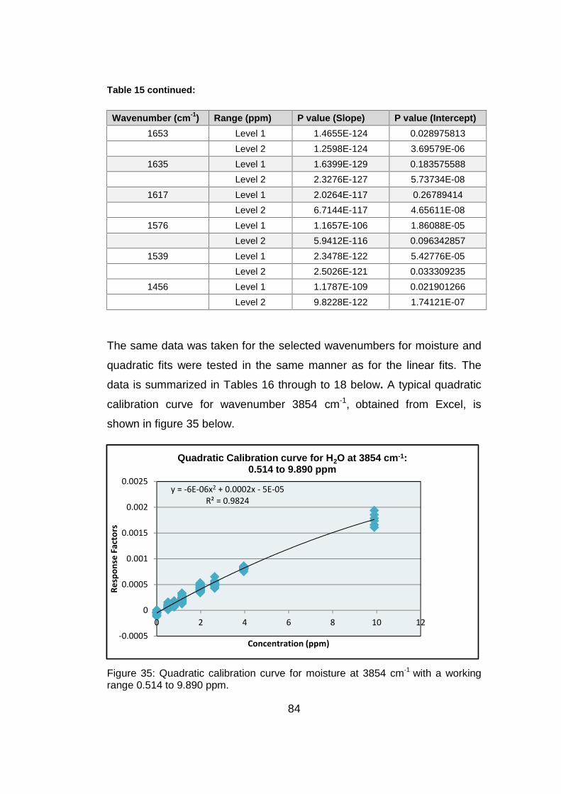
84

y = -6E-06x2 + 0.0002x - 5E-05R² = 0.9824

-0.0005

0

0.0005

0.001

0.0015

0.002

0.0025

0 2 4 6 8 10 12

Resp

onse

Fac

tors

Concentration (ppm)

Quadratic Calibration curve for H2O at 3854 cm-1:0.514 to 9.890 ppm

Table 15 continued:

Wavenumber (cm-1) Range (ppm) P value (Slope) P value (Intercept)1653 Level 1 1.4655E-124 0.028975813

Level 2 1.2598E-124 3.69579E-061635 Level 1 1.6399E-129 0.183575588

Level 2 2.3276E-127 5.73734E-081617 Level 1 2.0264E-117 0.26789414

Level 2 6.7144E-117 4.65611E-081576 Level 1 1.1657E-106 1.86088E-05

Level 2 5.9412E-116 0.0963428571539 Level 1 2.3478E-122 5.42776E-05

Level 2 2.5026E-121 0.0333092351456 Level 1 1.1787E-109 0.021901266

Level 2 9.8228E-122 1.74121E-07

The same data was taken for the selected wavenumbers for moisture and

quadratic fits were tested in the same manner as for the linear fits. The

data is summarized in Tables 16 through to 18 below. A typical quadratic

calibration curve for wavenumber 3854 cm-1, obtained from Excel, is

shown in figure 35 below.

Figure 35: Quadratic calibration curve for moisture at 3854 cm-1 with a workingrange 0.514 to 9.890 ppm.

85

Table 16: Summary of quadratic regression data for moisture standard:Regression data for t test

Wavenumber(cm-1)


3854 Level 1 0.9914 0.9829 90.62 1.98 4077.3Level 2 0.9849 0.9700 66.59 1.98 2200.6

3712 Level 1 0.9938 0.9877 107.86 1.98 5776.6Level 2 0.9919 0.9840 92.04 1.98 4205.3

3689 Level 1 0.9947 0.9895 116.39 1.98 6726.6Level 2 0.9926 0.9852 95.91 1.98 4565.7

1734 Level 1 0.9941 0.9882 109.99 1.98 6007.2Level 2 0.9916 0.9832 89.93 1.98 4014.6

1685 Level 1 0.9938 0.9876 107.31 1.98 5717.8Level 2 0.9912 0.9825 87.99 1.98 3842.6

1653 Level 1 0.9951 0.9902 120.87 1.98 7254.2Level 2 0.9927 0.9855 96.99 1.98 4668.9

1635 Level 1 0.9951 0.9903 121.15 1.98 7288.1Level 2 0.9933 0.9868 101.05 1.98 5068.3

1617 Level 1 0.9933 0.9866 103.02 1.98 5269.4Level 2 0.9903 0.9806 85.52 1.98 3462.3

1576 Level 1 0.9899 0.9799 83.778 1.98 3484.9Level 2 0.9894 0.9789 79.97 1.98 3174.2

1539 Level 1 0.9946 0.9893 115.47 1.98 6619.9Level 2 0.9919 0.9838 91.529 1.98 4158.4

1456 Level 1 0.9908 0.9817 88.03 1.98 3848.1Level 2 0.9924 0.9848 94.18 1.98 4402.9

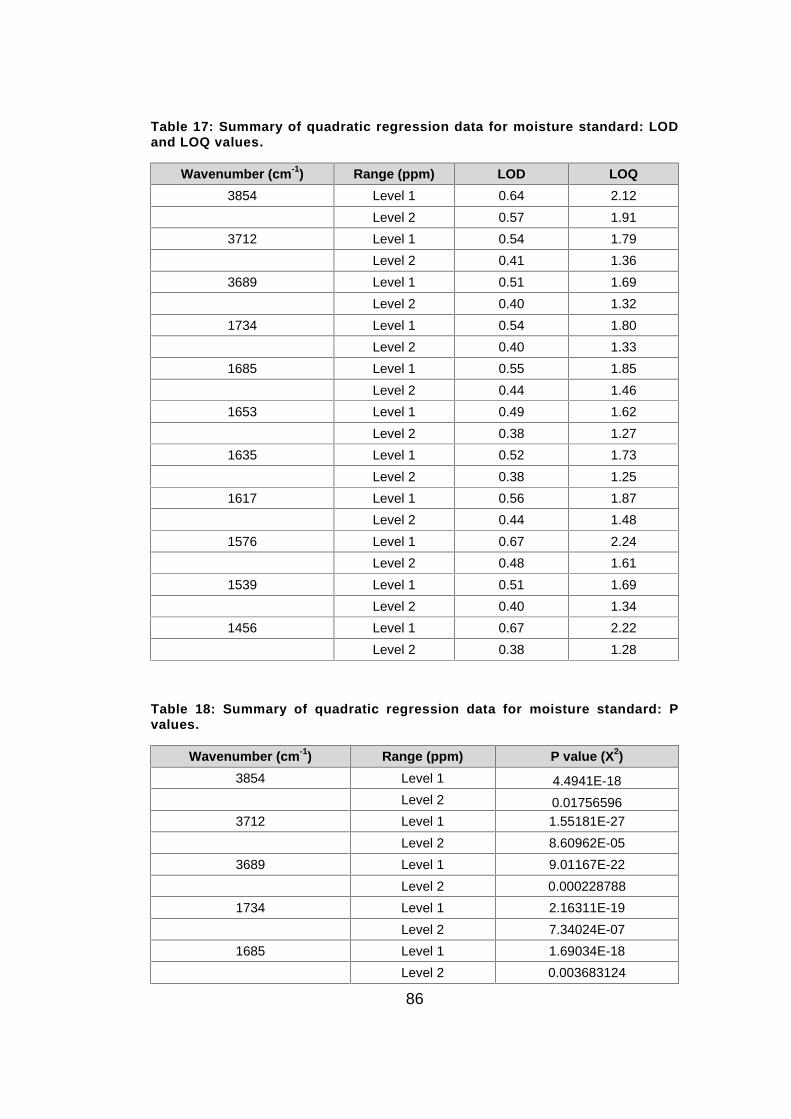
86

Table 17: Summary of quadratic regression data for moisture standard: LODand LOQ values.

Wavenumber (cm-1) Range (ppm) LOD LOQ3854 Level 1 0.64 2.12

Level 2 0.57 1.913712 Level 1 0.54 1.79

Level 2 0.41 1.363689 Level 1 0.51 1.69

Level 2 0.40 1.321734 Level 1 0.54 1.80

Level 2 0.40 1.331685 Level 1 0.55 1.85

Level 2 0.44 1.461653 Level 1 0.49 1.62

Level 2 0.38 1.271635 Level 1 0.52 1.73

Level 2 0.38 1.251617 Level 1 0.56 1.87

Level 2 0.44 1.481576 Level 1 0.67 2.24

Level 2 0.48 1.611539 Level 1 0.51 1.69

Level 2 0.40 1.341456 Level 1 0.67 2.22

Level 2 0.38 1.28

Table 18: Summary of quadratic regression data for moisture standard: Pvalues.

Wavenumber (cm-1) Range (ppm) P value (X2)3854 Level 1 4.4941E-18

Level 2 0.017565963712 Level 1 1.55181E-27

Level 2 8.60962E-053689 Level 1 9.01167E-22

Level 2 0.0002287881734 Level 1 2.16311E-19

Level 2 7.34024E-071685 Level 1 1.69034E-18

Level 2 0.003683124

87

y = 0.0007x + 8E-05R² = 0.997

0

0.0005

0.001

0.0015

0.002

0.0025

0.003

0.0035

0 1 2 3 4 5

Resp

onse

Fac

tors

Concentration (ppm)

Linear Calibration curve for CH4 at 3017 cm-1:Range 0.198 to 4.729 ppm

Table 15 continued:

Wavenumber (cm-1) Range (ppm) P value (X2)1653 Level 1 1.05348E-23

Level 2 1.17574E-051635 Level 1 6.80292E-19

Level 2 0.0001399871617 Level 1 5.81156E-21

Level 2 0.0001586261576 Level 1 5.30763E-19

Level 2 0.0083274211539 Level 1 4.46555E-23

Level 2 1.56245E-051456 Level 1 4.7751E-19

Level 2 3.88367E-06

Determining the suitability of methane as internal standard4.2.

A calibration curve with a regression of 0.997 was obtained for methane

using a linear fit and 0.999 using a quadratic fit. See figures 36 and 37

below.

Figure 36: Linear calibration curve for CH4 at 3017 cm-1 with a working rangebetween 0.198 and 4.729 ppm

88

y = -2E-05x2 + 0.0008x + 3E-05R² = 0.9992

0

0.0005

0.001

0.0015

0.002

0.0025

0.003

0.0035

0 1 2 3 4 5

Resp

onse

Fac

tors

Concentration (ppm)

Quadratic Calibration curve for CH4 at 3017 cm-1:Range 0.198 to 4.729 ppm

Figure 37: Quadratic calibration curve for CH4 at 3017 cm-1 with a working rangebetween 0.198 and 4.729 ppm

Visually the spread of results around each calibration point appeared to be

less than that obtained for the moisture tests indicating that the problem

with the spread of results around the moisture calibration levels was

related to the moisture itself and not the instrument. Moisture adheres to

the side walls of the glass cell despite heating of the cell and this could be

the cause of the spread of results around each calibration point for the

moisture. The spread of results around each calibration point for methane

was much less than the spread of results around each calibration point for

moisture indicating that methane does not adhere to the side walls of the

glass cell.

Methane as internal standard for moisture

The internal standard method allows the operating conditions to vary from

sample to sample without affecting the end results. The internal standard

must not be present in the unknown mixture and must not have any

unknown matrix effects. A known quantity of this internal standard is

added to the sample and any variation in sample size will be noticeable by

comparison of the response factors in different runs. (32)

89

Unfortunately the idea of using methane as internal standard with the

moisture permeation standard could not be implemented in this project.

The Matheson CH4 reference standard, imported from America, was very

expensive and due to the long equilibration times required for the

moisture, the scenario existed in which the CH4 reference standard would

be finished quite quickly. Since the CH4 is required as an internal standard

for ratio purposes, it does not have to be of as high a quality as the

Matheson CH4 reference standard. A more cost effective methane

standard possibly from a South African supplier such as Afrox will be

purchased and used to draw up a calibration curve for moisture using

methane as an internal standard.

To test the internal standard theory however, it was possible to use the

CH4 Matheson reference standard as an internal standard for the C2H2

calibration curves as the stabilization/equilibration times for C2H2 were

much less than those required for moisture.

Method 2: C2H2 analysis on FTIR4.3.

Calibration results for Standard 1: no internal standard

Calibration curves were set up using Standard 1 and the combination peak

at 1313 / 3249 cm-1 and the single peak at 1305 cm-1. The linear

calibration curves obtained from Excel for aforementioned wavenumbers

are shown in figures 39 and 40. The following concentrations were used

for both 3313/3266 and 1305 cm-1 (ppm): 33.550, 51.235, 76.733,

151.961, 246.815 and 369.048 ppm. All calculated parameters for the

calibration curves at the selected wavelengths are indicated in Tables 19

through to 22. The concentration ranges are classified as follows: Level 1:33.550 ppm to 369.0480 ppm and Level 2: 33.550 ppm to 246.815 ppm.

90

y = 6E-05x + 0.0001R² = 0.9965

-0.005

0

0.005

0.01

0.015

0.02

0.025

0 100 200 300 400

Resp

onse

fact

ors

Concentration (ppm)

Linear calibration curve for C2H2 at 1305 cm-1:Range 33.55 to 369.048 ppm

y = 2E-05x + 0.0005R² = 0.9876

00.0010.0020.0030.0040.0050.0060.0070.0080.009

0.01

0 100 200 300 400

Resp

onse

fact

ors

Concentration (ppm)

Linear calibration curve for C2H2 at 3313/3266 cm-1:Range 33.55 to 369.048 ppm

Figure 38: Linear calibration curve obtained for Standard 1 for C2H2 at 3313/3266cm-1

Figure 39: Linear calibration curve obtained for Standard 1 for C2H2 at 1305 cm-1

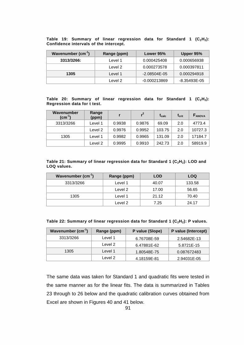
91

Table 19: Summary of linear regression data for Standard 1 (C2H2):Confidence intervals of the intercept.

Wavenumber (cm-1) Range (ppm) Lower 95% Upper 95%3313/3266: Level 1 0.000425408 0.000656938

Level 2 0.000273578 0.0003978111305 Level 1 -2.08504E-05 0.000294918

Level 2 -0.000213869 -8.35493E-05

Table 20: Summary of linear regression data for Standard 1 (C2H2):Regression data for t test.

Wavenumber(cm-1)


3313/3266 Level 1 0.9938 0.9876 69.09 2.0 4773.4Level 2 0.9976 0.9952 103.75 2.0 10727.3

1305 Level 1 0.9982 0.9965 131.09 2.0 17184.7Level 2 0.9995 0.9910 242.73 2.0 58919.9

Table 21: Summary of linear regression data for Standard 1 (C2H2): LOD andLOQ values.

Wavenumber (cm-1) Range (ppm) LOD LOQ3313/3266 Level 1 40.07 133.58

Level 2 17.00 56.651305 Level 1 21.12 70.40

Level 2 7.25 24.17

Table 22: Summary of linear regression data for Standard 1 (C2H2): P values.

Wavenumber (cm-1) Range (ppm) P value (Slope) P value (Intercept)3313/3266 Level 1 6.76708E-59 2.54682E-13

Level 2 6.47881E-62 5.8721E-151305 Level 1 1.80548E-75 0.087672483

Level 2 4.18159E-81 2.94031E-05

The same data was taken for Standard 1 and quadratic fits were tested in

the same manner as for the linear fits. The data is summarized in Tables

23 through to 26 below and the quadratic calibration curves obtained from

Excel are shown in Figures 40 and 41 below.

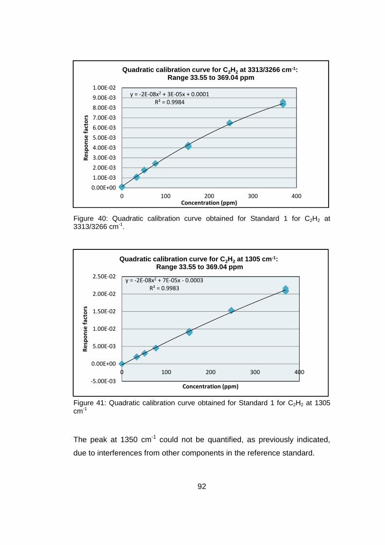
92

y = -2E-08x2 + 3E-05x + 0.0001R² = 0.9984

0.00E+001.00E-032.00E-033.00E-034.00E-035.00E-036.00E-037.00E-038.00E-039.00E-031.00E-02

0 100 200 300 400

Resp

onse

fact

ors

Concentration (ppm)

Quadratic calibration curve for C2H2 at 3313/3266 cm-1:Range 33.55 to 369.04 ppm

y = -2E-08x2 + 7E-05x - 0.0003R² = 0.9983

-5.00E-03

0.00E+00

5.00E-03

1.00E-02

1.50E-02

2.00E-02

2.50E-02

0 100 200 300 400

Resp

onse

fact

ors

Concentration (ppm)

Quadratic calibration curve for C2H2 at 1305 cm-1:Range 33.55 to 369.04 ppm

Figure 40: Quadratic calibration curve obtained for Standard 1 for C2H2 at3313/3266 cm-1.

Figure 41: Quadratic calibration curve obtained for Standard 1 for C2H2 at 1305cm-1

The peak at 1350 cm-1 could not be quantified, as previously indicated,

due to interferences from other components in the reference standard.

93

Table 23: Summary of quadratic regression data for Standard 1 (C2H2):Confidence intervals of the intercept.

Wavenumber (cm-1) Range (ppm) Lower 95% Upper 95%3313/3266 Level 1 5.90035E-05 0.000179881

Level 2 0.0004087 -0.0008143491305 Level 1 -0.000459578 -0.000139254

Level 2 -2.30221E-06 0.000121307

Table 24: Summary of quadratic regression data for Standard 1 (C2H2):Regression data for t test.

Wavenumber(cm-1)


3313/3266 Level 1 0.9992 0.9984 190.78 2.0 17895.9Level 2 0.9971 0.9941 102.47 2.0 5165.81

1305 Level 1 0.9991 0.9983 185.45 2.0 16909.9Level 2 0.9998 0.9997 391.05 2.0 74989.5

Table 25: Summary of quadratic regression data for Standard 1 (C2H2): LODand LOQ values.


Level 2 13.60 45.341305 Level 1 13.04 43.48

Level 2 5.00 16.67

Table 26: Summary of quadratic Excel regression data for Standard 1 (C2H2):P values.

Wavenumber (cm-1) Range (ppm) P value (X2)3313/3266 Level 1 1.43584E-27

Level 2 3.54145E-111305 Level 1 1.95761E-10

Level 2 3.89607E-12


Calibration curves were set up using the in-house certified standard and

the combination peak at 3313 / 3266 cm-1 and the single peaks at 1350

94

y = 1E-05x + 0.0011R² = 0.9935

00.005

0.010.015

0.020.025

0.030.035

0 500 1000 1500 2000 2500 3000

Resp

onse

fact

ors

Concentration (ppm)


y = 4E-06x + 0.0002R² = 0.9965

-2.00E-03

0.00E+00

2.00E-03

4.00E-03

6.00E-03

8.00E-03

1.00E-02

1.20E-02

0 500 1000 1500 2000 2500 3000

Resp

onse

Fac

tors

Concentration (ppm)


cm-1 and 1305 cm-1 used for quantitation. Both linear and quadratic

selections were tested using Excel regression data. The results are

summarized in Tables 28 to 31 and the calibration curves shown in

Figures 42 to 44. The following concentrations (ppm) were used for both

3313/3266, 1350 and 1305 cm-1: 147.780, 243.740, 360.930, 446.870,

766.050, 1294.370 and 2681.190 ppm.

Figure 42: Linear calibration curve obtained for Standard 2 for C2H2 at 3313/3266cm-1


95

y = 4E-06x + 0.0002R² = 0.9965

-2.00E-03

0.00E+00

2.00E-03

4.00E-03

6.00E-03

8.00E-03

1.00E-02

1.20E-02

1.40E-02

0 500 1000 1500 2000 2500 3000

Resp

onse

Fac

tor

Concentration (ppm)



All calculated parameters for the calibration curves at the selected

wavelengths are indicated in Tables 27 through to 30 below. The

concentration ranges are classified as follows: Level 1: 147.780 ppm to

2681.190 ppm and Level 2: 147.780 ppm to 1294.370 ppm

Table 27: Summary of linear regression data for Standard 2 (C2H2):Confidence intervals of the intercept.

Wavenumber (cm-1) Range (ppm) Lower 95% Upper 95%3313/3266 Level 1 0.00088442 0.001326591

Level 2 0.000478288 0.0007907941350 Level 1 0.000181354 0.000295743

Level 2 8.4462E-05 0.0001542311305 Level 1 0.000150379 0.000261357

Level 2 7.11203E-05 0.000136962

96

Table 28: Summary of linear regression data for Standard 2 (C2H2):Regression data for t test.

Wavenumber(cm-1) Range (ppm) r r2 tcalc tcrit FANOVA

3313/3266 Level 1 0.9967 0.9933 102.07 2.0 10418.47Level 2 0.9970 0.9940 102.58 2.0 10523.58

1350 Level 1 0.9982 0.9965 139.45 2.0 19445.75Level 2 0.9987 0.9975 158.30 2.0 25057.31

1305 Level 1 0.9984 0.9968 147.43 2.0 21734.92Level 2 0.9989 0.9978 170.17 2.0 28958.22

Table 29: Summary of linear regression data for Standard 2 (C2H2): LOD andLOQ values.


Level 2 95.37 317.91350 Level 1 130.43 434.78

Level 2 61.62 205.401305 Level 1 123.37 411.24

Level 2 57.32 191.06

Table 30: Summary of linear regression data for Standard 2 (C2H2): P values.

Wavenumber (cm-1) Range (ppm) P value (Slope) P value (Slope)3313/3266 Level 1 6.80372E-78 4.4728E-15

Level 2 1.00621E-72 2.04018E-111350 Level 1 2.5378E-86 5.18137E-12

Level 2 1.20091E-83 3.84532E-091305 Level 1 5.52663E-88 2.47993E-10

Level 2 1.27258E-85 3.06535E-08


as for the linear fits. The data is summarized in Tables 31 to 34 below and

the quadratic calibration curves obtained from Excel are shown in Figures

45 to 47 below.

97

y = -1E-09x2 + 1E-05x + 0.0003R² = 0.9982

0.00E+00

5.00E-03

1.00E-02

1.50E-02

2.00E-02

2.50E-02

3.00E-02

3.50E-02

0 500 1000 1500 2000 2500 3000

Resp

onse

fact

ors

Concentration (ppm)


y = -2E-10x2 + 5E-06x + 5E-05R² = 0.9988

-2.00E-03

0.00E+00

2.00E-03

4.00E-03

6.00E-03

8.00E-03

1.00E-02

1.20E-02

0 500 1000 1500 2000 2500 3000

Resp

onse

Fac

tors

Concentration (ppm)


Figure 45: Quadratic calibration curve obtained for Standard 2 for C2H2 at3313/3266 cm-1


98

y = -2E-10x2 + 5E-06x + 4E-05R² = 0.9985

-2.00E-03

0.00E+00

2.00E-03

4.00E-03

6.00E-03

8.00E-03

1.00E-02

1.20E-02

1.40E-02

0 500 1000 1500 2000 2500 3000

Resp

onse

Fac

tors

Concentration (ppm)



Table 31: Summary of quadratic regression data for Standard 2 (C2H2):Confidence intervals (no internal standard)


Level 2 -0.0001090 9.59103E-051350 Level 1 2.2841E-07 9.34798E-05

Level 2 -3.686E-05 2.67931E-051305 Level 1 -1.268E-05 9.59851E-05

Level 2 -3.836E-05 2.86994E-05

Table 32: Summary of quadratic regression data for Standard 2 (C2H2):Regression data for t test (no internal standard)

Wavenumber(cm-1)


3313/3266 Level 1 0.9991 0.9982 199.26 2.0 19568.37Level 2 0.9994 0.9989 239.10 2.0 28137.30

1350 Level 1 0.9994 0.9988 242.22 2.0 28909.26Level 2 0.9995 0.9991 263.36 2.0 34127.96

1305 Level 1 0.9992 0.9985 213.11 2.0 22379.20Level 2 0.9995 0.9990 253.55 2.0 31633.92

99

Table 33: Summary of quadratic regression data for Standard 2 (C2H2): LODand LOQ values (no internal standard)


Level 2 32.87 109.561350 Level 1 65.61 218.37

Level 2 32.60 108.651305 Level 1 76.12 253.75

Level 2 34.45 114.84

Table 34: Summary of quadratic regression data for Standard 2 (C2H2): Pvalues (no internal standard)


Level 2 9.09852E-251350 Level 1 6.27893E-18

Level 2 2.58555E-151305 Level 1 1.8312E-12

Level 2 2.55682E-12


Calibration curves were once again set up using the in-house certified

standard and the combination peak at 13313 / 3266 cm-1 and the single

peaks at 1350 cm-1 and 1305 cm-1 used for quantitation. CH4 was used as

internal standard and the methane peak at 3017 cm-1 used for

quantitation. Both linear and quadratic selections were tested using

Microsoft Excel software. The results are summarized in Tables 35 to 38

and the calibration curves shown in Figures 48 to 50. The following

concentrations (ppm) were used for 3313/3266, 1350 and 1305 cm-1:

194.137, 319.387, 380.807, 357.867, 421.319, 535.189 and 596.445 ppm.

The concentration ranges are classified as follows: Level 1: 194.137 ppm

to 596.445 ppm and Level 2: 194.137 ppm to 535.1890 ppm

100

y = 0.0089x + 0.1961R² = 0.9937

0

1

2

3

4

5

6

0 100 200 300 400 500 600 700

Resp

onse

fact

ors

Concentration (ppm)


y = 0.0025x + 0.0402R² = 0.996

00.20.40.60.8

11.21.41.61.8

0 100 200 300 400 500 600 700

Resp

onse

fact

ors

Concentration (ppm)


C2H2

Figure 48: Linear calibration curve obtained for Standard 2 for C2H2 at 3313/3266cm-1 using CH4 as internal standard.


using CH4 as internal standard.

101

y = 0.004x + 0.1429R² = 0.9852

0

0.5

1

1.5

2

2.5

3

0 100 200 300 400 500 600 700

Resp

onse

fact

ors

Concentration (ppm)




Table 35: Summary of linear regression data for Standard 2 (C2H2):Confidence intervals (with internal standard)


Level 2 0.08430639 0.2209870031350 Level 1 0.02304273 0.052207036

Level 2 0.01404659 0.0444487571305 Level 1 0.09112652 0.179604735

Level 2 0.06273288 0.152891778

Table 36: Summary of linear regression data for Standard 2 (C2H2):Regression data for t test (with internal standard)

Wavenumber(cm-1)


3313/3266 Level 1 0.9968 0.9937 107.07 2.0 11463.62Level 2 0.9966 0.9933 96.40 2.0 9292.582

1350 Level 1 0.9980 0.9961 137.74 2.0 18971.98Level 2 0.9978 0.9957 121.27 2.0 14707.64

1305 Level 1 0.9928 0.9858 72.08 2.0 5194.969Level 2 0.9927 0.9854 66.20 2.0 4382.004

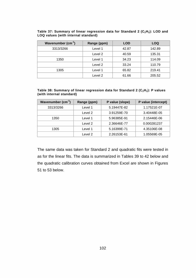
102

Table 37: Summary of linear regression data for Standard 2 (C2H2): LOD andLOQ values (with internal standard)


Level 2 40.59 135.311350 Level 1 34.23 114.09

Level 2 33.24 110.791305 Level 1 65.82 219.41

Level 2 61.66 205.52

Table 38: Summary of linear regression data for Standard 2 (C2H2): P values(with internal standard)

Wavenumber (cm-1) Range (ppm) P value (slope) P value (intercept)3313/3266 Level 1 5.19447E-82 1.17521E-07

Level 2 3.91259E-70 3.40448E-051350 Level 1 5.96385E-91 2.15446E-06

Level 2 2.36646E-77 0.0002812371305 Level 1 5.16399E-71 4.35106E-08

Level 2 2.26153E-61 1.05569E-05




51 to 53 below.

103

y = -3E-06x2 + 0.0109x + 0.0044R² = 0.9994

0

1

2

3

4

5

6

0 100 200 300 400 500 600 700

Resp

onse

fact

ors

Concentration (ppm)


y = -7E-07x2 + 0.003x - 0.0012R² = 0.9994

-0.20

0.20.40.60.8

11.21.41.61.8

0 100 200 300 400 500 600 700

Resp

onse

fact

ors

Concentration (ppm)


Figure 51: Quadratic calibration curve obtained for Standard 2 for C2H2 at3313/3266 cm-1 using CH4 as internal standard.

Figure 52: Quadratic calibration curve obtained for Standard 2 for C2H2 at 1350cm-1 using CH4 as internal standard.

104

y = -2E-06x2 + 0.0054x + 0.0106R² = 0.9989

0

0.5

1

1.5

2

2.5

3

0 100 200 300 400 500 600 700

Resp

onse

fact

ors

Concentration (ppm)

Quadratic calibration curve for C2H2 at 1305 cm-1:Range 194.137to 596.445 ppm


Table 39: Summary of quadratic regression data for Standard 2 (C2H2):Confidence intervals (with internal standard)

Wavenumber (cm-1) Range (ppm) Lower 95% Upper 95%3313/3266 Level 1 -0.0207010 0.02947818

Level 2 -0.0215348 0.0069509841350 Level 1 3.8363E-05 0.00085136

Level 2 -4.422E-05 0.0007082851305 Level 1 -0.0041123 0.025320269

Level 2 -0.0028631 0.009960539

Table 40: Summary of quadratic regression data for Standard 2 (C2H2):Regression data for t test (with internal standard)

Wavenumber(cm-1)


3313/3266 Level 1 0.9997 0.9994 351.09 2.0 60788.83Level 2 0.9999 0.9998 545.38 2.0 146359.9

1350 Level 1 0.9997 0.9993 347.51 2.0 59562.54Level 2 0.9998 0.9996 411.84 2.0 83481.32

1305 Level 1 0.9995 0.9989 264.92 2.0 34623.66Level 2 0.9999 0.9998 545.64 2.0 146569.3

105

Table 41: Summary of quadratic regression data for Standard 2 (C2H2): LODand LOQ values (with internal standard)


Level 2 5.86 19.521350 Level 1 11.68 38.93

Level 2 8.33 27.771305 Level 1 13.47 44.88

Level 2 5.58 18.62

Table 42: Summary of quadratic regression data for Standard 2 (C2H2): Pvalues (with internal standard)


Level 2 2.72658E-481350 Level 1 5.22739E-31

Level 2 4.2033E-351305 Level 1 2.29859E-43

Level 2 3.74658E-60


Calibration curves were set up using Standard 3. The combination peak at

13313 / 3266 cm-1 and the single peaks at 1350 cm-1 and 1305 cm-1 were

used for quantitation. Both linear and quadratic selections were tested

using Excel software. The results are summarized in Tables 43 to 46 and

the calibration curves shown in Figures 55 to 56. The following


94.804, 155.968, 185.962, 205.745, 230.238, 261.35 and 291.265 ppm.

The concentration ranges are classified as follows: Level 1: 94.804 ppm to

291.265 ppm and Level 2: 94.804 ppm to 261.265 ppm

106

y = 4E-05x + 0.0007R² = 0.9846

-0.002

0

0.002

0.004

0.006

0.008

0.01

0.012

0.014

0.016

0 100 200 300 400

Resp

onse

fact

ors

Concentration (ppm)


y = 0.0001x + 0.0017R² = 0.9869

-0.0050

0.0050.01

0.0150.02

0.0250.03

0.0350.04

0 100 200 300 400

Resp

onse

fact

ors

Concentration (ppm)


Figure 54: Linear calibration curve for Standard 3 for C2H2 at 1313/3266 cm-1 witha working range between 94.804 and 291.265 ppm

Figure 55: Linear calibration curve for Standard 3 for C2H2 at 1305 cm-1 with aworking range between 94.804 and 291.265 ppm

107

y = 4E-05x + 0.0007R² = 0.9853

0

0.002

0.004

0.006

0.008

0.01

0.012

0.014

0.016

0 50 100 150 200 250 300 350

Resp

onse

fact

ors

Concentration (ppm)

Linear Calibration curve for C2H2 at 1305 cm-1:Range 94.804 to 291.265 ppm

Figure 56: Linear calibration curve for Standard 3 for C2H2 at 1350 cm-1 with aworking range between 94.804 and 291.265 ppm

Table 43: Summary of linear regression data for Standard 3 (C2H2):Confidence intervals (no internal standard)


Level 2 0.00071569 0.0020491391350 Level 1 0.00045900 0.000977111

Level 2 0.00028313 0.0008107351305 Level 1 0.00047042 0.000969695

Level 2 0.00030628 0.000819745

Table 44: Summary of linear regression data for Standard 3 (C2H2):Regression data for t test (no internal standard)

Wavenumber(cm-1)


3313/3266 Level 1 0.9938 0.9876 75.26 2.0 5664.0Level 2 0.9939 0.9879 71.11 2.0 5056.7

1350 Level 1 0.9927 0.9856 28.69 2.0 4842.8Level 2 0.9928 0.9856 65.15 2.0 4244.9

1305 Level 1 0.9931 0.9863 71.43 2.0 5103.0Level 2 0.9930 0.9860 66.09 2.0 4367.4

108

Table 45: Summary of linear regression data for Standard 3 (C2H2): LOD andLOQ values (no internal standard)


Level 2 24.37 81.22350 Level 1 28.69 95.63

Level 2 26.60 88.651305 Level 1 27.95 93.16

Level 2 26.22 87.40

Table 46: Summary of linear regression data for Standard 3 (C2H2): P values(no internal standard)

Wavenumber (cm-1) Range (ppm) P value (slope) P value (intercept)3313/3266 Level 1 1.85805E-69 4.82942E-07

Level 2 3.85989E-61 0.0001050071350 Level 1 4.4888E-67 5.07866E-07

Level 2 8.16328E-59 0.0001051231305 Level 1 7.18204E-68 2.06572E-07

Level 2 3.42094E-59 4.59395E-05




57 to 59 below.

109

y = -5E-08x2 + 6E-05x - 9E-05R² = 0.9945

-2.00E-03

0.00E+00

2.00E-03

4.00E-03

6.00E-03

8.00E-03

1.00E-02

1.20E-02

1.40E-02

0 50 100 150 200 250 300 350

Resp

onse

fact

ors

Concentration (ppm)


y = -1E-07x2 + 0.0002x - 0.0002R² = 0.9952

-5.00E-03

0.00E+00

5.00E-03

1.00E-02

1.50E-02

2.00E-02

2.50E-02

3.00E-02

3.50E-02

4.00E-02

0 50 100 150 200 250 300 350

Resp

onse

fact

ors

Concentration (ppm)


Figure 57: Quadratic calibration curve for Standard 3 for C2H2 at 1313/3266 cm-1

with a working range between 94.804 and 291.265 ppm

Figure 58: Quadratic calibration curve for Standard 3 for C2H2 at 1350 cm-1 with aworking range between 94.804 and 291.265 ppm

110

y = -5E-08x2 + 6E-05x - 6E-05R² = 0.9948

-2.00E-03

0.00E+00

2.00E-03

4.00E-03

6.00E-03

8.00E-03

1.00E-02

1.20E-02

1.40E-02

0 50 100 150 200 250 300 350

Resp

onse

fact

ors

Concentration (ppm)

Quadratic Calibration curve for C2H2 at 1305cm-1: Range94.804 to 291.265 ppm

Figure 59: Quadratic calibration curve for Standard 3 for C2H2 at 1305 cm-1 with aworking range between 94.804 and 291.265 ppm

Table 47: Summary of quadratic regression data for Standard 3 (C2H2):Confidence intervals (no internal standard)


Level 2 -0.0008143 0.00040871350 Level 1 -0.0002939 0.000137445

Level 2 -0.0003358 0.0001191241305 Level 1 -0.0004116 0.000163365

Level 2 -0.0002999 0.000136153

Table 48: Summary of quadratic regression data for Standard 3 (C2H2):Regression data for t test (no internal standard)

Wavenumber(cm-1)


3313/3266 Level 1 0.9975 0.9950 117.90 2.0 6850.5Level 2 0.9971 0.9941 102.47 2.0 5165.8

1350 Level 1 0.9973 0.9946 114.77 2.0 6493.3Level 2 0.9969 0.9938 99.103 2.0 4890.8

1305 Level 1 0.9974 0.9949 117.29 2.0 6781.1Level 2 0.9970 0.9942 102.69 2.0 5187.2

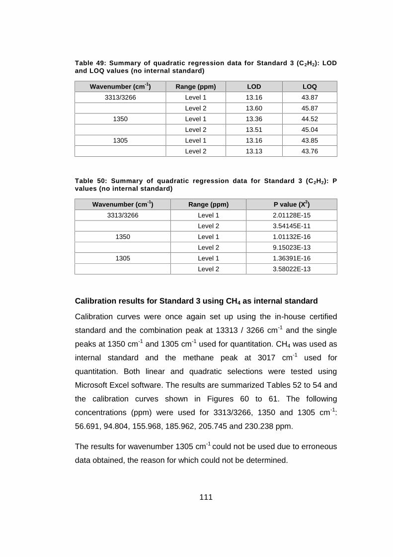
111

Table 49: Summary of quadratic regression data for Standard 3 (C2H2): LODand LOQ values (no internal standard)


Level 2 13.60 45.871350 Level 1 13.36 44.52

Level 2 13.51 45.041305 Level 1 13.16 43.85

Level 2 13.13 43.76

Table 50: Summary of quadratic regression data for Standard 3 (C2H2): Pvalues (no internal standard)


Level 2 3.54145E-111350 Level 1 1.01132E-16

Level 2 9.15023E-131305 Level 1 1.36391E-16

Level 2 3.58022E-13


Calibration curves were once again set up using the in-house certified

standard and the combination peak at 13313 / 3266 cm-1 and the single

peaks at 1350 cm-1 and 1305 cm-1 used for quantitation. CH4 was used as

internal standard and the methane peak at 3017 cm-1 used for

quantitation. Both linear and quadratic selections were tested using

Microsoft Excel software. The results are summarized Tables 52 to 54 and

the calibration curves shown in Figures 60 to 61. The following


56.691, 94.804, 155.968, 185.962, 205.745 and 230.238 ppm.

The results for wavenumber 1305 cm-1 could not be used due to erroneous

data obtained, the reason for which could not be determined.

112

y = 0.002x + 0.0139R² = 0.9924

0

0.1

0.2

0.3

0.4

0.5

0.6

0 50 100 150 200 250

Resp

onse

fact

ors

Concentration (ppm)

Linear calibration curve for C2H2 at 1313/3266 cm-1 with Istd:Range 56.691 to 230.238 ppm

y = 0.0007x - 0.0028R² = 0.9926

-0.020

0.020.040.060.08

0.10.120.140.160.18

0 50 100 150 200 250

Resp

onse

fact

ors

Concentration (ppm)

Linear calibration curve for C2H2 at 1350 cm-1 with Istd:Range 56.691 to 230.238 ppm

Figure 60: Linear calibration curve obtained for Standard 3 for C2H2 at 3313/3266cm-1 using CH4 as internal standard.



113

Table 51: Summary of linear regression data for Standard 3 (C2H2):Confidence intervals (with internal standard)


Level 2 0.00584642 0.0200449921350 Level 1 -0.0047636 -0.00045907

Level 2 -0.0045340 -3.8981E-05

Table 52: Summary of linear regression data for Standard 3 (C2H2):Regression data for t test (with internal standard)

Wavenumber(cm-1)


3313/3266 Level 1 0.9961 0.9924 91.18 2.0 8313.781Level 2 0.9956 0.9913 78.96 2.0 6235.102

1350 Level 1 0.9964 0.9929 94.30 2.0 8891.707Level 2 0.9958 0.9916 80.67 2.0 6508.163

Table 53: Summary of linear regression data for Standard 3 (C2H2): LOD andLOQ values (with internal standard)


Level 2 20.97 69.891350 Level 1 20.22 67.41

Level 2 20.52 68.41

Table 54: Summary of Linear regression data for Standard 3 (C2H2): P values(with internal standard)

Wavenumber (cm-1) Range (ppm) P value (slope) P value (intercept)3313/3266 Level 1 1.80468E-69 0.000128463

Level 2 2.68233E-58 0.0005767341350 Level 1 2.13415E-70 0.018194373

Level 2 8.33504E-59 0.046287699


as for the linear fits using internal standard. The data is summarized in

114

y = 2E-07x2 + 0.0006x - 0.0017R² = 0.9928

-0.020

0.020.040.060.08

0.10.120.140.160.18

0 50 100 150 200 250

Resp

onse

fact

ors

Concentration (ppm)

Quadratic calibration curve for C2H2 at 1350 cm-1 with internalstandard:

Range 56.691 to 230.238 ppm

y = -2E-06x2 + 0.0024x + 0.0027R² = 0.9948

0

0.1

0.2

0.3

0.4

0.5

0.6

0 50 100 150 200 250

Resp

onse

fact

ors

Concentration (ppm)

Quadratic calibration curve for C2H2 at 1313/3266 cm-1 withinternal std:

Range 56.691 to 230.238 ppm

Tables 47 to 50 below and the quadratic calibration curves obtained from

Excel are shown in Figures 62 to 63 below.

Figure 62: Quadratic calibration curve obtained for Standard 3 for C2H2 at3313/3266 cm-1 using CH4 as internal standard.


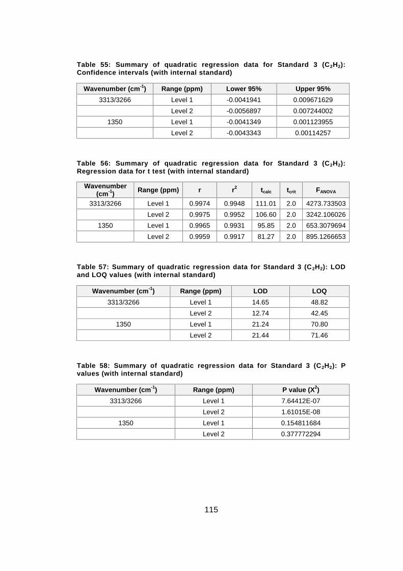
115

Table 55: Summary of quadratic regression data for Standard 3 (C2H2):Confidence intervals (with internal standard)


Level 2 -0.0056897 0.0072440021350 Level 1 -0.0041349 0.001123955

Level 2 -0.0043343 0.00114257

Table 56: Summary of quadratic regression data for Standard 3 (C2H2):Regression data for t test (with internal standard)

Wavenumber(cm-1) Range (ppm) r r2 tcalc tcrit FANOVA

3313/3266 Level 1 0.9974 0.9948 111.01 2.0 4273.733503Level 2 0.9975 0.9952 106.60 2.0 3242.106026

1350 Level 1 0.9965 0.9931 95.85 2.0 653.3079694Level 2 0.9959 0.9917 81.27 2.0 895.1266653

Table 57: Summary of quadratic regression data for Standard 3 (C2H2): LODand LOQ values (with internal standard)


Level 2 12.74 42.451350 Level 1 21.24 70.80

Level 2 21.44 71.46

Table 58: Summary of quadratic regression data for Standard 3 (C2H2): Pvalues (with internal standard)


Level 2 1.61015E-081350 Level 1 0.154811684

Level 2 0.377772294

116

Statistics4.4.

Linear regression analyses

A linear regression line equation generally takes the form:

Y = b0 + b1x

Where Y = Dependent variable

b0 = Intercept

b1 = Slope

x = variable

The sample slope (b1) is given in the “Coefficients” column and the “X

Variable/Slope” row. The estimated change in y as a result of a one unit

change in x is measured by b1.

The intercept b0 is given in the “Coefficients” column and the “Intercept (Y)”

row and b0 is the estimated value of y when x is 0.

Evaluating the results of the regression analysis

Excel software was used to determine the linear regression parameters.

The interpretations of each of the more common parameters are

discussed below.

Plot of the residuals

A plot of the residuals can be used to determine possible problems with

the calibration data that may not be immediately obvious from a simple

scatter plot of the data.

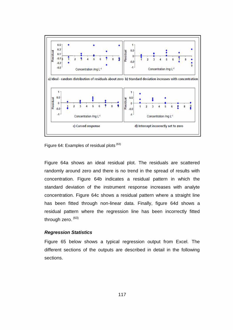
117

Figure 64: Examples of residual plots (63)

Figure 64a shows an ideal residual plot. The residuals are scattered

randomly around zero and there is no trend in the spread of results with

concentration. Figure 64b indicates a residual pattern in which the

standard deviation of the instrument response increases with analyte

concentration. Figure 64c shows a residual pattern where a straight line

has been fitted through non-linear data. Finally, figure 64d shows a

residual pattern where the regression line has been incorrectly fitted

through zero. (63)

Regression Statistics

Figure 65 below shows a typical regression output from Excel. The

different sections of the outputs are described in detail in the following

sections.

118

SUMMARY OUTPUT

Regression StatisticsMultiple R (r) 0.984806789R Square (r2) 0.969844412Adjusted R Square 0.969633534Standard Error (sy/x) 6.78578E-05Observations (n) 145

ANOVAdf SS MS F Significance F

Regression 1 2.11773E-05 2.11773E-05 4599.07308 1.2731E-110Residual 143 6.5847E-07 4.60469E-09Total 144 2.18358E-05

Coefficients Standard Error t Sta/tcalc P-value Lower 95% Upper 95% Lower 95.0% Upper 95.0%Intercept (Y) 8.03487E-06 8.01446E-06 1.002546421 0.31777319 -7.80725E-06 2.3877E-05 -7.80725E-06 2.3877E-05X variable/Slope 0.000189649 2.7965E-06 67.81646615 1.2731E-110 0.000184121 0.000195177 0.000184121 0.000195177

↑ (b)Tcrit = (TINV(, n-2)

Figure 65: Typical excel regression data. Red/bold data indicates componentsused in calculations.

The correlation coefficient (r)

The correlation coefficient (r) and the related, parameters r2 and adjusted

r2, are measures of how strong the correlation is between the x and the y

values. The closer r is to 1, the stronger the correlation but unfortunately

the r value can be easily misinterpreted. It is therefore essential to plot

calibration data and not to just rely on the statistics. The parameters r2 and

adjusted r2 are used to describe the fraction of total variance in the data

which can be contributed to by the line that has been fitted. The majority of

the variability can be accounted for by the fitted line if there is a good

linear relation and r2 should thus be close to 1. The adjusted r2 is

interpreted in the same manner as r2 but is always lower. It is a useful

parameter for assessing the effect of adding additional terms to the

equation of the fitted line if for example a quadratic fit is used instead of a

linear fit. Where r2 always increases on the addition of extra terms to the

equation, adjusted r2 takes into account the reduction in the in the degrees

of freedom which occurs every time an additional term is added and thus

119

does not automatically increase on addition of extra terms. This prevents

over fitting which can occur when the equation fitted has more terms than

can be supported by the amount of data available. (63)

ANOVA Table

ANOVA is defined as “analysis of variance”. Figure 65 illustrates the origin

of some of the terms from an ANOVA table. The sum of squares (SS)

indicates different sources of variability in the calibration data. The

regression term represents the variability in the data that can be

accounted for by the fitted regression line. Ideally the larger this term, the

greater the linearity as the fitted line will describe most of the variability in

response with concentration. The residual term is the sum of the squared

residuals and this value should be small compared to the regression sum

of squares as the residuals will be small if the regression line fits the data

well. The mean square (MS) for both regression and residual is the sum of

squares divided by its degrees of freedom. The F value is the ratio of the

regression term MS term to the residual MS and should ideally be very

large if there is a good linear relationship. The significance F value

represents the probability of obtaining the results in the ANOVA table if

there is no correlation between x and y values, more simply put, the

results are obtained by chance. A small value would indicate that the

results were unlikely to have happened by chance this indicating the

likelihood that there is a strong relationship between the x and y values. F

Significance should be extremely small for a calibration curve to be of any

use. (63)

Regression coefficients

The final table in the ANOVA table from figure 65 describes the regression

outputs. The first column provides the values of the coefficients followed

by the second column which gives the standard errors for each coefficient.

These values provide the ranges within which the values for the gradient

and intercept could be found. Related to these values are the values in the

120

last columns, lower and upper 95% confidence limits. These values

represent the extremes of the values that gradient and intercept could take

at a chosen confidence level, 95% for the work done in this project. The t-

stat and p-values relate to the significance of the coefficients and provide

an indication of whether the coefficients are statistically significant from

zero. The expectation is that the gradient of a line be significantly different

from zero and thus the t-value must be large and the p-value must be

small, typically less than 0.05 for a regression analyses carried out at the

95% level. Ideally it is preferred that the calibration line pass through the

origin. If this is the case then the intercept should not be significantly

different from zero. It would thus be expected that the t-value would be

small and the p-value would be large, typically greater than 0.05 at the

95% confidence level. A final confirmation of whether the calibration line

passes through zero is to assess the upper and lower confidence intervals.

If these two values include zero then the intercept is not statistically

different from zero. (63)

Discussion on results for linear calibration data H2O

Does r represent significant linearity?

A t-test was performed here as follows:

The hypotheses are as follows:

H0: r = 0 and there is no linear relation between x and y

H1: r ≠ 0 and there is significant linearity

If tcalc > tcrit then reject H0 and there is significant linearity. The bigger tcalc,,

the more significant the linearity. All 11 wavenumbers in both ranges had

tcalc > tcrit, indicating significant linearity for all. In only two cases were the

tcalc values of the higher ranges better than the lower ranges and that was

for 3854 and 1734 cm-1. An Anova analysis was then performed in Exel to

determine if the lower ranges indicated greater linearity than the higher

121

ranges. FANOVA was compared with Fcrit and the FANOVA with the highest

value was selected as the more linear range. (64) In all cases excluding

3854 and 1734 cm-1, the lower ranges displayed higher values for FANOVA

indicating more significant linearity for the lower ranges than for the higher

ranges.

Discussion on results for quadratic calibration data H2O

The tcalc and FANOVA values for all eleven wavenumbers were all higher for

the high ranges than for the low ranges indicating that a quadratic fit is the

better option on the high range. The r2 values on the high ranges were

also better than the r2 values obtained for the linear fits indicating that for

moisture analyses it is perhaps better to use a quadratic calibration curve

rather than the linear option.

Discussion on results for calibration data C2H2 for Standard 1

Visual examination of the graphs for Standard 1 indicated that the

quadratic fit for wavenumber 3313/3266 cm-1 was a more probable fit than

the linear fit while 1305 cm-1 could be either fit. The tcalc and FANOVA values

on the linear low range were both larger than the tcalc and FANOVA values

on the linear high range indicating that the lower range has more linearity

than the high range on the linear fits. The tcalc and FANOVA values on the

quadratic high range for 3313/3266 cm-1 was larger than the tcalc and

FANOVA values on the quadratic low range indicating that the high range is a

better quadratic fit than the low range on the quadratic fits. However for

wavenumber 1305 cm-1, the tcalc and FANOVA values on the quadratic low

range was larger than the tcalc and FANOVA values on the quadratic high

range indicating that the low range is a better quadratic fit than the high

range on the quadratic fits.



quadratic fit for wavenumber 3313/3266 cm-1 was again a more probable

122

fit than the linear fit while 1305 cm-1 and 1305 cm-1 could be either fit. The

tcalc and FANOVA values on all three linear low ranges were both larger than

the tcalc and FANOVA values on the linear high ranges indicating that the

lower ranges have more linearity than the high ranges on the linear fits.

The tcalc and FANOVA values on the quadratic low ranges for all three

wavenumbers were larger than the tcalc and FANOVA values on the quadratic

high ranges indicating, strangely enough, that the low ranges are a better

quadratic fit than the high ranges on the quadratic fits. Considering the r2

values for both linear and quadratic fits, the r2 values for the quadratic fits

were better than for the linear fits.

The use of internal standard made a significant difference to the r2 values

obtained on the quadratic ranges but did not seem to have a great effect

on the linear fits.



quadratic fits for all three wavenumbers was a more probable fit than the

linear fit. The tcalc and FANOVA values on all three linear high ranges were

both larger than the tcalc and FANOVA values on the linear low ranges

indicating that the high ranges have more linearity than the low ranges on

the linear fits. This is opposite to what we found on Standard 2. The tcalc

and FANOVA values on the quadratic high ranges for all three wavenumbers

were larger than the tcalc and FANOVA values on the quadratic low ranges

indicating, that the high ranges are a better quadratic fit than the low

ranges on the quadratic fits. Considering the r2 values for both linear and

quadratic fits, the r2 values for the quadratic fits were better than for the

linear fits.

The use of internal standard made a small difference to the r2 values

obtained on both the linear and quadratic ranges but did not seem to have

as great an effect as it did for standard 2.

123

Method 3: analysis on GC/PDHID4.5.

Calibration results for C2H2

A method was developed for the analysis of acetylene in a difficult matrix.

The matrix was removed so as not to have an effect on the PDHID signal

allowing for quicker stabilization times of the GC/PDHID system. A

calibration curve was drawn up for acetylene using this method. No

statistical evaluation was undertaken for the calibration data as was done

for the FTIR analyses. The reason for this is that acetylene is a compound

commonly run on GC and is known to be linear. In addition it was decided

not to spend further time on this method as the conversion of H2O to C2H2

could not be further investigated due to the lack of a proper sealed

sampling unit for the conversion process.

Conversion of moisture to C2H24.6.

It was determined that the conversion process from H2O to C2H2 was

viable. Unfortunately a number of factors put a stop to any further

development of this process. The CaC2 purchased was found to contain

H2O and also rapidly reacted with H2O when exposed to air. This resulted

in much higher % recoveries for the C2H2 than initially anticipated. Purging

the vials/sample holder with helium prior to the conversion process

appeared to remove the additional moisture/ C2H2 present as the

recoveries improved but due to air ingress, specifically into the sample

holder, no viable results could be obtained.

124

In Summary4.7.

The purpose of this project was the development of a method (s) by which

to analyze the moisture content of gas samples. The Water Gas Shift

reaction could not be tested due to the unavailability of the catalysts. Two

methods were developed. Initially the FTIR was selected and a method

developed whereby moisture could be directly analyzed. Eleven calibration

curves, using eleven different wavenumbers, were set up using a moisture

permeation standard and an initial working range from 0.514 to 9.890

ppm. Visual inspection of the calibration curves gave the impression that

the curves all tended towards quadratic fits. The full range was then split

into an additional smaller range of 0.514 to 3.956 ppm. The smaller range

proved to have a more linear fit than the full range which tended towards a

quadratic fit.

The disadvantages of this method included long stabilization times for

each calibration level, at least four hours per level, and when it came to

sample analyses, large volumes of sample were required for analyses

making it an impractical method for any samples other than cylinders

containing large volumes and/or high pressures of gas. The long

stabilization times for both standards and samples were largely due to the

long path gas cell being constructed of glass and the moisture adsorbing

to the glass walls thus indicating that a long path glass gas cell is not

suitable for the direct analyses of moisture in gases. Heating the glass cell

did not improve desorption of the water on the glass walls but actually

appeared to increase the amount of moisture present.

The second method developed for the analyses of the moisture content of

gas samples also utilized FTIR. For this method various calibration curves

were set up for acetylene with the purpose of quantifying moisture in gas

samples, after conversion to acetylene. Standard 1 (Matheson) was used

as a preliminary test and data was generated. There were however many

interferences from all the additional components in the mixture and only

125

two of the 3 wavenumbers (3313/3266 and 1305 cm-1) selected could be

used for calibration. The concentration range used was from 33.550 to

369.048 ppm. The ranges were split into a smaller range as for the

moisture calibrations but no significant difference could be seen between

the higher and lower ranges. The quadratic fit gave a better r2 value for

every wavenumber.

Standard 2 provided a calibration range from 147.780 to 2681.19 ppm

without internal standard and a range from 194.137 to 596.445 ppm with

internal standard. There was a definite improvement in r2 with the use of

internal standard on the linear range as well as the quadratic range.

Standard 3 provided a calibration range from 94.804 to 291.265 ppm

without internal standard and a range from 56.691 to 230.238 ppm with

internal standard. Again there was a definite improvement in r2 with the

use of internal standard on the linear range as well as the quadratic range.

A calibration curve for acetylene was drawn up using GC/PDHID. This is a

standard analyses and it was decided not to spend additional time on the

GC method until the conversion process could be confidently

implemented.

The principle of the conversion of moisture to acetylene using calcium

carbide was tested. The conversion process was proven to be successful

but it could not be quantified at the close of this project due to the lack of a

sealed sample holder. Calcium carbide proved to be very reactive to

moisture and any small ingress of air caused the conversion process to

occur resulting in much higher recoveries than anticipated.

No references could be found in literature as to the use of quadratic

calibration curves versus linear calibration curves. In most instances from

literature, linear regression was used.(9) Additionally no references could

be found regarding the use of an internal standard for the FTIR technique.

126

In table 59 below, a number of techniques and the detection limits

obtained are summarized.

Table 59: Comparison of moisture measurement techniques (1)

Technique Gases tested Sensitivity/DetectionLimits

Comment

FTIR Cl2, HCl, HBr, NH3,AsH3 and PH3

10-50ppbv Background H2O inbench affects response.

TDLASHCl, HBr, NH3,H2,O2, Inerts, N2O,CO and SiH4

1-10ppbvDetection at low Prequired to keeplinewidth narrow.

CRDS N2, HCl <500ppt High mirror reflectivityrequired.

ILS N2, HCl <500ppt Low resolution may limitapplications

MS Inerts, N2, HCl andWF6

500ppbv. Varies withmatrix

Detector drifts

APIMS Inerts, O2, GeH4,SiH4, NH3 and HCl

10ppt-10ppv. Varieswith matrix

Complex-requires skilledoperator and regularmaintenance

OscillatingQuartzcrystal

O2, H2, NO, CO,Hydrocarbons,inerts, AsH3, PH3,SF6 and NH3

10-50ppbvRequires dry referencegas and periodiccalibration.

Chilled mirror HCl, HBr, PH3 andAsH3

Varies Long equilibration timesat low H2O levels

CapacitanceCO, halocarbons,N2O, inerts, PH3and AsH3

>100ppbvRequires frequentcalibration at low H2Olevels

ElectrolyticCl2, inerts, SF6,CO, CO2 andfreons

2-5ppbv and 1ppmvin Cl2

Precise flow controlrequired. Dry cell maynot respond to H2O

The detection limits for moisture obtained in this project (on average

0.5ppm) are greater than those obtained from the various techniques

illustrated in table 59. The FTIR LOD indicated in table 59 does not give an

indication of the type of detector or cell used and can thus not be directly

compared to the method set up in this project. It would seem that the long

path glass cell used for this project has its limitations and is possibly not

suitable if detection limits less than 0.5ppm are required.

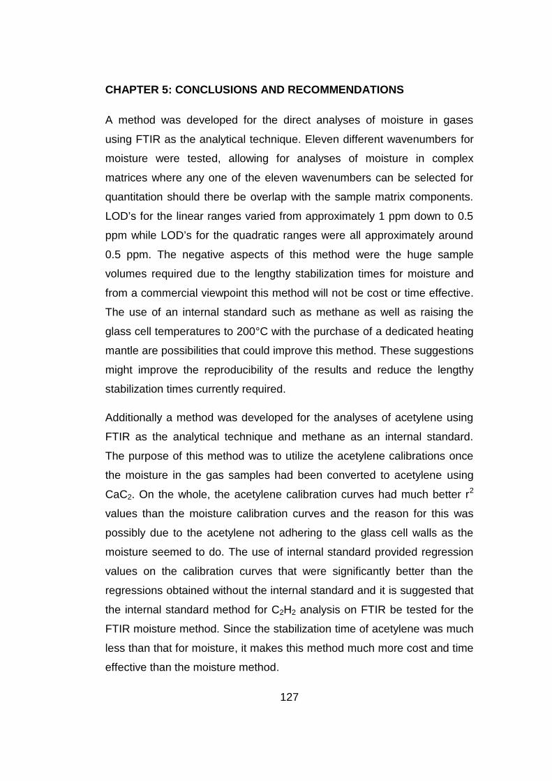
127

CHAPTER 5: CONCLUSIONS AND RECOMMENDATIONS

A method was developed for the direct analyses of moisture in gases

using FTIR as the analytical technique. Eleven different wavenumbers for

moisture were tested, allowing for analyses of moisture in complex

matrices where any one of the eleven wavenumbers can be selected for

quantitation should there be overlap with the sample matrix components.

LOD’s for the linear ranges varied from approximately 1 ppm down to 0.5

ppm while LOD’s for the quadratic ranges were all approximately around

0.5 ppm. The negative aspects of this method were the huge sample

volumes required due to the lengthy stabilization times for moisture and

from a commercial viewpoint this method will not be cost or time effective.

The use of an internal standard such as methane as well as raising the

glass cell temperatures to 200°C with the purchase of a dedicated heating

mantle are possibilities that could improve this method. These suggestions

might improve the reproducibility of the results and reduce the lengthy

stabilization times currently required.

Additionally a method was developed for the analyses of acetylene using

FTIR as the analytical technique and methane as an internal standard.

The purpose of this method was to utilize the acetylene calibrations once

the moisture in the gas samples had been converted to acetylene using

CaC2. On the whole, the acetylene calibration curves had much better r2

values than the moisture calibration curves and the reason for this was

possibly due to the acetylene not adhering to the glass cell walls as the

moisture seemed to do. The use of internal standard provided regression

values on the calibration curves that were significantly better than the

regressions obtained without the internal standard and it is suggested that

the internal standard method for C2H2 analysis on FTIR be tested for the

FTIR moisture method. Since the stabilization time of acetylene was much

less than that for moisture, it makes this method much more cost and time

effective than the moisture method.

128

The principle of the conversion of moisture to acetylene was proved in this

study but no quantification could be done due to the lack of a sealed

sample holder. A sample holder for both GC and FTIR in which moisture in

a gas sample can be converted to acetylene using calcium carbide,

without the ingress of atmospheric air/moisture needs to be developed.

The design of such a sample holder is crucial to the success of the

conversion process. In addition to the air ingress into the sample holder,

the sealed CaC2 container from the supplier, opened for use for the first

time for the conversion process contained acetylene indicating some air

ingress prior to sealing of the container. This could be removed to an

extent by purging with helium. It is recommended that the CaC2 be stored

under an inert gas and when transferring the CaC2 to the sample holder

AND that this be done under an inert gas to prevent air ingress and thus

higher acetylene results than expected. 70% purity CaC2 was utilized for

these experiments. It is possible that a higher purity grade CaC2 might

contain less H2O/C2H2 and provide more accurate conversion results.

129

REFERENCES

1. Funke, H. et al. Techniques for the measurement of trace moisture in

high-purity electronic speciality gases, Review of Scientific Instruments,

vol. 74, no 9, 2003, pp. 3909-3933.

2. Geiger, W.M. and Raynor, M.W. Trace analysis of specialty and

electronic gases, New Jersey, Wiley, 2012. ISBN 978-1-118-06566-2.

3. Snyder, S. FTIR Analytical method for NF3, Arizona, BOC Gases, 1998.

4. de Coning, J P. Validation of the determination of moisture in helium by

FTIR, Brits, Pelindaba Analytical Labs, 2003.

5. Kim, S. H. et al. Analysis of natural gas using single capillary column

and a pulsed discharge helium ionization detector, Bull. Korean chem. Soc

Korea, vol. 20, no 7, Oct 1999, pp. 843-845.

6. Wentworth, W.E. et al. Pulsed discharge helium ionization detector,

Journal of Chromatograpia, vol. 34, no 5-8, 1992, pp. 219-225.

7. Roberge, M.T. et al. Evaluation of the pulsed discharge helium

ionization detector for the analysis of hydrogen and methane in breath,

Journal of Chromatography A, Elsevier, vol. 1027, no 1-2, 2004, pp. 19-23.

8. Weijun, Y. Trace Analysis of impurities in bulk gases by gas

chromatography-pulsed discharge helium ionization detection with "heart

cutting" technique, Journal of Chromatography A, Elsevier, vol 1167, no 2,

2007, pp. 225-230.

9. Espinoza, L. H. et al. Trace water vapor determination in nitrogen and

corrosive gases using infrared spectroscopy. Sandia Corporation.

Albuquerque, Sandia National Laboratories, 1997.

10. Forbes, J W. Trace water determination by infrared spectroscopy,

California, Analytical chemistry, vol. 34, no 9, 1962, pp. 1125-1128.

130

11. Badoni, A. and Jayaraman, R.P. Determination of the water content in

organic compounds by gas chromatography using back flush technique,

Dehradun, India, Springer.com, Fresnius Journal of Analytical Chemistry,

vol. 338, no 6, Nov 1990, pp. 745-748.

12. Agency California Environment Protection. Standard operating

procedure for water determination in consumer products using gas

chromatography, California, 2003. MLD SOP SAS04.

13. Jalbert, J. Gilbert, R. and Tetreault, P. Simultaneous determination of

dissolved gases and moisture in mineral insulating oils by static

headspace gas chromatography with helium photoionization pulsed

discharge detection, Canada, IREQ, Analytical Chemistry, vol. 73, no 14,

July 15, 2001, pp. 3382-3391.

14. New World Encyclopedia Contributors. Friedrich Wohler. New World

Encyclopedia. April 2008, [Accessed: November 21, 2013]

http://www.newworldencyclopedia.org/p/index.php?title=Friedrich_W%C3

%B6hler&oldid=684286

15. Bustamante, F. et al. Kinetic study of the reverse water gas shift

reaction in high-temperature, high pressure homogenous systems.

Pittsburgh, 2002. [Accessed: November 21, 2013]

http://web.anl.gov/PCS/acsfuel/preprint%20archive/Files/47_2_Boston_10-

02_0274.pdf

16. Luengnaruemitchai, A. Osuwan, S. and Gulari, E. Comparative studies

of low-temperature water-gas shift reaction over Pt/CeO2, Au/CeO2, and

Au/Fe2O3 catalysts, Elsevier, Catalysis Communications, vol. 4, March

13, 2003, pp. 215-221.

17. Sun, H. Wang, B and DiMagno, S.G. A method for detecting water in

organic solvents. Nebraska, Organic Letters, vol. 10, no 20, July 8, 2008,

pp. 4413-4416.

131

18. Smith, B. Loganathan, M. and Shanta, M.S. A review of the water gas

shift reaction kinetics. The Berkley Electronic Press, International Journal

of Chemical Reactor Engineering, vol. 8, 2010, pp. 1-34.

19. Nexant. PERP Program - Acetylene production technologies.

[Accessed: July 26, 2013]

http://thinking.nexant.com/sites/default/files/report/field_attachment_abstra

ct/200704/0506S9_abs.pdf

20. NIOSH. Biological effects of exposure. The national Institute for

Occupational Safety and Health (NIOSH). [Accessed: July 26, 2013]

http://www.cdc.gov/niosh/pdfs/76-195b.pdf

21. Colorado University. Infrared spectroscopy theory, Online edition for

students of organic chemistry lab courses at the University of Colorado,

Boulder, Dept of Chem and Biochem. [Accessed: June 10, 2013]

http://orgchem.colorado.edu/Spectroscopy/irtutor/IRtheory.pdf

22. Perez, J.E. and Meyer, R.T. FTIR spectroscopy. CIC Photonics.

1994. [Accessed: October 11, 2013]

www.irgas.com/ftir_spectroscopy.html

23. Robotics fundamental series. Infrared, 2008. [Accessed: March 3,

2013] http://www.ni.com/whitepaper/8225/en

24. Materialscientist, Wikipedia, Infrared spectroscopy. [Accessed:

February 2, 2013.] http://en.wikipedia.org/wiki/Infrared spectroscopy.

25. Molecular vibrations and infrared spectroscopy. [Accessed: March 3,

2013] www.chem.ucla.edu/harding/ec_tutorials/tutorial31.pdf

26. Sheffield Hallam University, Infrared absorption spectroscopy -

Theoretical Principles. [Accessed: March 3, 2013]

http://teaching.shu.ac.uk/hwb/chemistry/tutorials/molspec/irspec

132

27. Reusch, W. Infrared Spectroscopy. [Accessed: March 3, 2013]

http://www2.chemistry.msu.edu/faculty/reusch/virttxtjml/spectrpy/infrared/in

frared.htm

28. Settle, F. et al. Handbook of instrumental techniques for analytical

chemistry, Upper Saddle River, NJ: Prentice Hall PTR, 1997, pp. 249,

ISBN: 0131773380 9780131773387

29. Stuart, B. Infrared Spectroscopy: Fundamentals and Applications.

Australia, Wiley, 2004. pp. 19-20. ISBN: 978-0-470-85428-0.

30. Newport Corporation. Introduction to FTIR Spectroscopy. [Accessed:

March 12, 2013] http://www.newport.com/Introduction-to-FT-IR-

Spectroscopy/405840/1033/content.aspx

31. Amand, L. and Tullin, C.J. The theory behind FTIR analyses.

[Accessed: March 12, 2013]

http://turroserver.chem.columbia.edu/pdf_db/theory_ftir.pdf

32. Willard, H. et al. Instrumental methods of analysis. California,

Wadsworth Publishing Company, 1988. pp. 189-191. ISBN: 0-534-

245021.

33. Rogalski, A. Infrared detectors: An Overview. Poland, Elsevier,

Infrared Physics and Technology, No 43, 2002, pp. 187-210.

34. Fukudu, H. Using infrared detectors-MCT detector, FTIR Talk Letter

Shimadzu. April 2010. Vol 13. [Accessed: November 6, 2013]

http://www.shimadzu.com/an/ftir_talk/index.html

35. Spectratech. [Accessed: October 02, 2014] http://www.kinecat.pl

36. Edmund Optics Inc. The Correct Material for Infrared (IR) Applications,

Edmund Optics Inc. [Accessed: October 02, 2014]

http://www.edmundoptics.com

133

37. Vaughan, S. and Vaughan, W. FTIR Analytical systems: Part II-

Experimental design, Gases & Instrumentation International, Jan/Feb

2009, [Accessed: October 24, 2013]

www.gasesmag.com/articles.php?pid=58

38. Shimadzu. Measurement methods for gas samples. Shimadzu,

Excellence in Science. [Accessed: March 12, 2013]

www.shimadzu.com/an/ftir/support/ftirtalk/talk13/intro.html

39. Coates, J. Vibrational Spectroscopy: Instrumentation for Infrared and

Raman Spectroscopy, Newtown, USA, Coates Consulting, 1998, Applied

Spectroscopy Reviews, vol. 33, no 4, pp. 267-425.

40. Gas phase analysis of water using FTIR. [Accessed: June 2013]

https://www.pacelabs.com

41. Nishikida, K. Nishio, E. and Hannah, R.W. Selected applications of

modern FT-IR techniques. Luxembourg, Gordon and Breach Science

Publishers S.A., 1995. ISBN 2-88449-073-6.

42. Skoog, D. A, Holler, J.E. and Crouch, S.R. Principles of Instrumental

Analysis. Canada, David Harris, 2007. pp. 762-808. ISBN-13:978-0-495-

01201-6.

43. Scott, R.P.W. Principles and practice of chromatography. [Accessed:

August 27, 2013] http://www.library4science.com

44. Kupiec, T. Quality-control analytical methods: Gas chromatography,

Oklahoma , 2004, International Journal of Pharmaceutical compounding,

vol. 8, no 4, pp. 305-309.

45. D.A. Skoog, D.M. West. Fundamentals of analytical chemistry, Holt,

Rinehart and Winston, 1967, ISBN 0-03-089495-6.

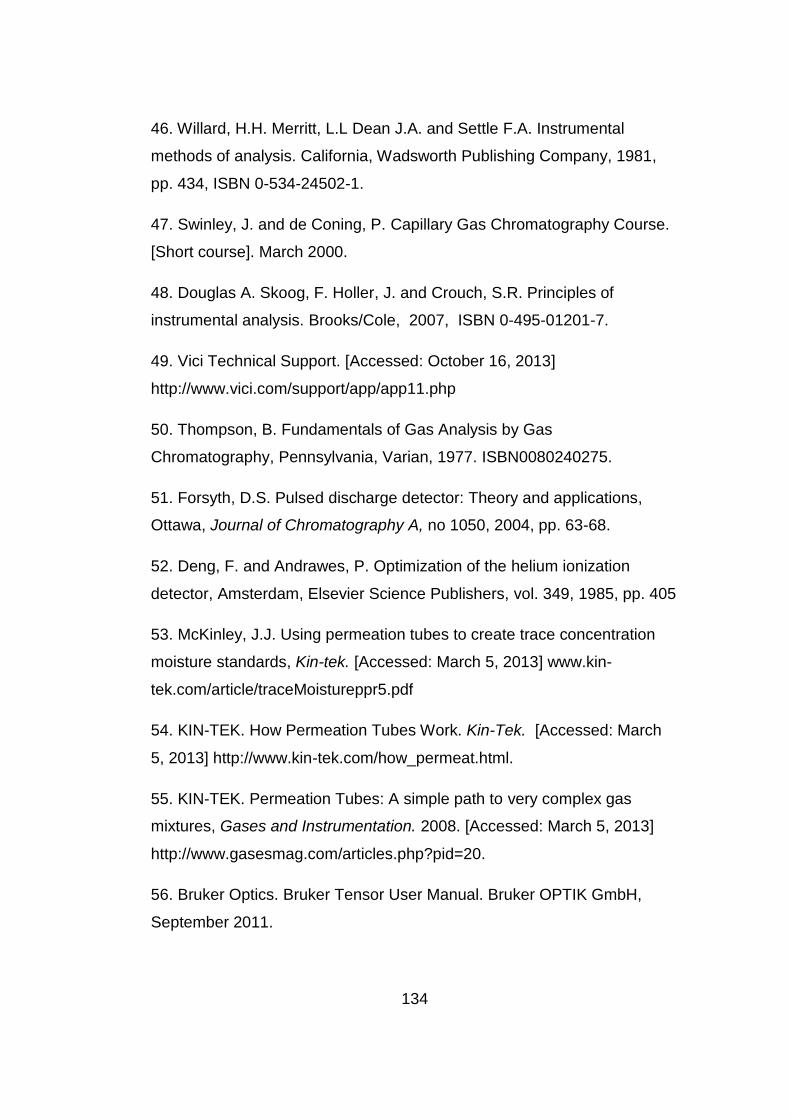
134

46. Willard, H.H. Merritt, L.L Dean J.A. and Settle F.A. Instrumental

methods of analysis. California, Wadsworth Publishing Company, 1981,

pp. 434, ISBN 0-534-24502-1.

47. Swinley, J. and de Coning, P. Capillary Gas Chromatography Course.

[Short course]. March 2000.

48. Douglas A. Skoog, F. Holler, J. and Crouch, S.R. Principles of

instrumental analysis. Brooks/Cole, 2007, ISBN 0-495-01201-7.

49. Vici Technical Support. [Accessed: October 16, 2013]

http://www.vici.com/support/app/app11.php

50. Thompson, B. Fundamentals of Gas Analysis by Gas

Chromatography, Pennsylvania, Varian, 1977. ISBN0080240275.

51. Forsyth, D.S. Pulsed discharge detector: Theory and applications,

Ottawa, Journal of Chromatography A, no 1050, 2004, pp. 63-68.

52. Deng, F. and Andrawes, P. Optimization of the helium ionization

detector, Amsterdam, Elsevier Science Publishers, vol. 349, 1985, pp. 405

53. McKinley, J.J. Using permeation tubes to create trace concentration

moisture standards, Kin-tek. [Accessed: March 5, 2013] www.kin-

tek.com/article/traceMoistureppr5.pdf

54. KIN-TEK. How Permeation Tubes Work. Kin-Tek. [Accessed: March

5, 2013] http://www.kin-tek.com/how_permeat.html.

55. KIN-TEK. Permeation Tubes: A simple path to very complex gas

mixtures, Gases and Instrumentation. 2008. [Accessed: March 5, 2013]

http://www.gasesmag.com/articles.php?pid=20.

56. Bruker Optics. Bruker Tensor User Manual. Bruker OPTIK GmbH,

September 2011.

135

57. VICI Metronics. Generating calibration gas standards with Dynacal

permeation devices: Technical Note 1001, [Accessed: September 15,

2014] www.vici.com/support/tn/tn1001.pdf

58. Laboratories, KIN-TEK. Trace Source TM Permeation Tubes LFH

Operations Manual. Texas

59. VICI: Technical Support. VICI. [Online] [Accessed: August 5, 2013.]

www.vici.com/support/app/app2j.php

60. VICI: Tecnical Support. VICI. [Online] [Accessed: August 5, 2013.]

www.vici.com/support/app/app6j.php

61. VICI: Technical Support. VICI. [Online] [Accessed: September 17,

2013.] http://www.vici.com/support/app/app12j.php

62. Barwick, V. Preparation of Calibration Curves: A Guide to best

practice, Department of Trade and Industry, 2003. [Accessed January

2015] www.lgcgroup.com/LGCGroup/media/PDFs

63. Chandler-Gilbert Community College Learning Center, Analyzing linear

regression with Excel. [Accessed: January 2015]

https://www.cgc.maricopa.edu/Academics/LearningCenter/Math/Document

s/AnalyzingLinearRegression.pdf.

136

APPENDIX 1:

Trace Source Permeation Tube Certificate of Calibration

137

y = 0.0002x + 5E-05R² = 0.9719

-5.00E-04

0.00E+00

5.00E-04

1.00E-03

1.50E-03

2.00E-03

2.50E-03

0 10 20

Resp

onse

Fac

tors

Concentration (ppm)

Linear calibration curve for H2Oat 3712 cm-1

Range 0.514 to 9.890 ppm

y = 0.0003x - 2E-05R² = 0.9821

-2.00E-04

0.00E+00

2.00E-04

4.00E-04

6.00E-04

8.00E-04

1.00E-03

1.20E-03

0 5

Resp

onse

Fac

tors

Concentration (ppm)


Range 0.514 to 3.956 0 ppm

Range:0-9.89SUMMARY OUTPUT

Regression StatisticsMultiple R 0.985873948R Square 0.97194744Adjusted R Square 0.971753974Standard Error 8.2313E-05Observations 147



Coefficients Standard Error t Stat P-value Lower 95% Upper 95% Lower 95.0% Upper 95.0%Intercept 4.53597E-05 9.52746E-06 4.760943 4.61999E-06 2.65291E-05 6.41903E-05 2.65291E-05 6.41903E-05X Variable 1 0.000228072 3.21775E-06 70.87926 2.0165E-114 0.000221712 0.000234432 0.000221712 0.000234432

Range: 0-3.956SUMMARY OUTPUT




Coefficients Standard Error t Stat P-value Lower 95% Upper 95% Lower 95.0% Upper 95.0%Intercept -1.75661E-05 6.44905E-06 -2.72383 0.007287727 -3.03179E-05 -4.8144E-06 -3.03179E-05 -4.81437E-06X Variable 1 0.000269812 3.10471E-06 86.90419 2.2725E-122 0.000263673 0.000275951 0.000263673 0.000275951

APPENDIX 2:

Linear and Quadratic Calibration Data for all H2O wavenumbers:

138

y = -8E-06x2 + 0.0003x -4E-05

R² = 0.9877

-5.00E-04

0.00E+00

5.00E-04

1.00E-03

1.50E-03

2.00E-03

2.50E-03

0 5 10 15

Resp

onse

Fac

tors

Concentration (ppm)

Quadratic calibration curve forH2O at 3712 cm-1


y = -1E-05x2 + 0.0003x -4E-05

R² = 0.984

-2.00E-04

0.00E+00

2.00E-04

4.00E-04

6.00E-04

8.00E-04

1.00E-03

1.20E-03

0 2 4 6

Resp

onse

Fac

tors

Concentration (ppm)







Coefficients Standard Error t Stat P-value Lower 95% Upper 95% Lower 95.0% Upper 95.0%Intercept -4.06424E-05 8.95977E-06 -4.5361 1.19781E-05 -5.8352E-05 -2.2933E-05 -5.8352E-05 -2.29327E-05X Variable 1 0.000305157 6.06998E-06 50.27317 3.24234E-93 0.00029316 0.000317155 0.00029316 0.000317155X Variable 2 -8.45574E-06 6.23125E-07 -13.5699 1.55181E-27 -9.68739E-06 -7.2241E-06 -9.68739E-06 -7.22408E-06






139

y = 0.0002x + 2E-05R² = 0.9799

-5.00E-04

0.00E+00

5.00E-04

1.00E-03

1.50E-03

2.00E-03

0 5 10 15

Resp

onse

Fac

tors

Concentration (ppm)



y = 0.0002x - 2E-05R² = 0.9837

-2.00E-04-1.00E-040.00E+001.00E-042.00E-043.00E-044.00E-045.00E-046.00E-047.00E-048.00E-049.00E-04

0 5

Resp

onse

Fac

tors

Concentration (ppm)


Range 0.514 to 3.956 0 ppm





Coefficients Standard Error t Stat P-value Lower 95% Upper 95% Lower 95.0% Upper 95.0%Intercept 1.73039E-05 5.80356E-06 2.98160015 0.003367965 5.83273E-06 2.87751E-05 5.83273E-06 2.87751E-05X Variable 1 0.000170492 2.03202E-06 83.90293975 3.727E-124 0.000166476 0.000174509 0.000166476 0.000174509






140

y = -5E-06x2 + 0.0002x - 3E-05

R² = 0.9895

-5.00E-04

0.00E+00

5.00E-04

1.00E-03

1.50E-03

2.00E-03

0 5 10 15

Resp

onse

Fac

tors

Concentration (ppm)



y = -6E-06x2 + 0.0002x -3E-05

R² = 0.9852-2.00E-04-1.00E-040.00E+001.00E-042.00E-043.00E-044.00E-045.00E-046.00E-047.00E-048.00E-049.00E-04

Resp

onse

Fac

tors

Concentration (ppm)












Coefficients Standard Error t Stat P-value Lower 95% Upper 95% Lower 95.0% Upper 95.0%Intercept -3.36161E-05 6.20876E-06 -5.4143 2.67778E-07 -4.58935E-05 -2.1339E-05 -4.58935E-05 -2.13387E-05X Variable 1 0.000219637 7.37843E-06 29.76744 1.12067E-61 0.000205047 0.000234227 0.000205047 0.000234227X Variable 2 -6.48498E-06 1.7132E-06 -3.78531 0.000228788 -9.87271E-06 -3.0973E-06 -9.87271E-06 -3.09726E-06

141

y = 0.0001x + 2E-06R² = 0.9792

-2.00E-04

0.00E+00

2.00E-04

4.00E-04

6.00E-04

8.00E-04

1.00E-03

1.20E-03

1.40E-03

1.60E-03

0 10 20

Resp

onse

Fac

tors

Concentration (ppm)



y = 0.0002x - 3E-05R² = 0.9799

-2.00E-04

-1.00E-04

0.00E+00

1.00E-04

2.00E-04

3.00E-04

4.00E-04

5.00E-04

6.00E-04

7.00E-04

Resp

onse

Fac

tors

Concentration (ppm)

Linear Calibration curve for H2Oat 1734 cm-1






Coefficients Standard Error t Stat P-value Lower 95% Upper 95% Lower 95.0% Upper 95.0%Intercept 1.58388E-06 5.06933E-06 0.312443613 0.755155405 -8.43603E-06 1.16038E-05 -8.43603E-06 1.16038E-05X Variable 1 0.000146225 1.77494E-06 82.38312 4.9135E-123 0.000142717 0.000149733 0.000142717 0.000149733





Coefficients Standard Error t Stat P-value Lower 95% Upper 95% Lower 95.0% Upper 95.0%Intercept -2.56737E-05 4.15865E-06 -6.173565 7.00E-09 -3.38966E-05 -1.7451E-05 -3.38966E-05 -1.74508E-05X Variable 1 0.000164306 2.00206E-06 82.06834329 5.2867E-119 0.000160347 0.000168264 0.000160347 0.000168264

142

y = -4E-06x2 + 0.0002x -4E-05

R² = 0.9882

-2.00E-04

0.00E+00

2.00E-04

4.00E-04

6.00E-04

8.00E-04

1.00E-03

1.20E-03

1.40E-03

1.60E-03

0 10 20

Resp

onse

Fac

tors

Concentration (ppm)



y = -8E-06x2 + 0.0002x -5E-05

R² = 0.9832

-2.00E-04

-1.00E-04

0.00E+00

1.00E-04

2.00E-04

3.00E-04

4.00E-04

5.00E-04

6.00E-04

7.00E-04

0 5

Resp

onse

Fac

tors

Concentration (ppm)













143

y = 0.0001x - 7E-08R² = 0.9788

-2.00E-04

0.00E+00

2.00E-04

4.00E-04

6.00E-04

8.00E-04

1.00E-03

1.20E-03

1.40E-03

0 10 20

Resp

onse

Fac

tors

Concentration (ppm)



y = 0.0001x - 2E-05R² = 0.981

-1.00E-04

0.00E+00

1.00E-04

2.00E-04

3.00E-04

4.00E-04

5.00E-04

6.00E-04

0 5

Resp

onse

Fac

tors

Concentration (ppm)







Coefficients Standard Error t Stat P-value Lower 95% Upper 95% Lower 95.0% Upper 95.0%Intercept -7.35897E-08 4.25183E-06 -0.017307748 0.986215062 -8.47766E-06 8.33048E-06 -8.47766E-06 8.33048E-06X Variable 1 0.000121381 1.48871E-06 81.5343873 2.116E-122 0.000118438 0.000124323 0.000118438 0.000124323






144

y = -3E-06x2 + 0.0002x -3E-05

R² = 0.9876

-2.00E-04

0.00E+00

2.00E-04

4.00E-04

6.00E-04

8.00E-04

1.00E-03

1.20E-03

1.40E-03

0 5 10 15

Resp

onse

Fac

tors

Concentration (ppm)



y = -4E-06x2 + 0.0002x -3E-05

R² = 0.9825-1.00E-04

0.00E+00

1.00E-04

2.00E-04

3.00E-04

4.00E-04

5.00E-04

6.00E-04

0 5

Resp

onse

Fac

tors

Concentration (ppm)













145

y = 0.0002x + 2E-05R² = 0.9802

-5.00E-04

0.00E+00

5.00E-04

1.00E-03

1.50E-03

2.00E-03

2.50E-03

3.00E-03

0 10 20

Resp

onse

Fac

tors

Concentration (ppm)



y = 0.0003x - 3E-05R² = 0.983

-2.00E-04

0.00E+00

2.00E-04

4.00E-04

6.00E-04

8.00E-04

1.00E-03

1.20E-03

0 5

Resp

onse

Fac

tors

Concentration (ppm)













146

y = -7E-06x2 + 0.0003x -5E-05

R² = 0.9902

-5.00E-04

0.00E+00

5.00E-04

1.00E-03

1.50E-03

2.00E-03

2.50E-03

3.00E-03

0 5 10 15

Resp

onse

Fac

tors

Concentration (ppm)



y = -1E-05x2 + 0.0003x -6E-05

R² = 0.9855

-2.00E-04

0.00E+00

2.00E-04

4.00E-04

6.00E-04

8.00E-04

1.00E-03

1.20E-03

0 2 4 6

Resp

onse

Fac

tors

Concentration (ppm)













147

y = 0.0002x + 9E-06R² = 0.9831

-5.00E-04

0.00E+00

5.00E-04

1.00E-03

1.50E-03

2.00E-03

2.50E-03

0 10 20

Resp

onse

Fac

tors

Concentration (ppm)



y = 0.0002x - 3E-05R² = 0.9853

-2.00E-04

0.00E+00

2.00E-04

4.00E-04

6.00E-04

8.00E-04

1.00E-03

0 2 4 6

Resp

onse

Fac

tors

Concentration (ppm)













148

y = -5E-06x2 + 0.0002x -4E-05

R² = 0.9903

-5.00E-04

0.00E+00

5.00E-04

1.00E-03

1.50E-03

2.00E-03

2.50E-03

0 10 20

Resp

onse

Fac

tors

Concentration (ppm)



y = -7E-06x2 + 0.0003x -5E-05

R² = 0.9868

-2.00E-04

0.00E+00

2.00E-04

4.00E-04

6.00E-04

8.00E-04

1.00E-03

0 2 4 6

Resp

onse

Fac

tors

Concentration (ppm)













149

y = 0.0002x + 7E-06R² = 0.9751

-2.00E-040.00E+002.00E-044.00E-046.00E-048.00E-041.00E-031.20E-031.40E-031.60E-031.80E-03

0 5 10 15

Resp

onse

Fac

tors

Concentration (ppm)



y = 0.0002x - 3E-05R² = 0.978

-2.00E-04-1.00E-040.00E+001.00E-042.00E-043.00E-044.00E-045.00E-046.00E-047.00E-048.00E-04

0 2 4 6

Resp

onse

Fac

tors

Concentration (ppm)













150

y = -5E-06x2 + 0.0002x -4E-05

R² = 0.9866

-2.00E-040.00E+002.00E-044.00E-046.00E-048.00E-041.00E-031.20E-031.40E-031.60E-031.80E-03

0 5 10 15

Resp

onse

Fac

tors

Concentration (ppm)



y = -7E-06x2 + 0.0002x -5E-05

R² = 0.9806

-2.00E-04-1.00E-040.00E+001.00E-042.00E-043.00E-044.00E-045.00E-046.00E-047.00E-048.00E-04

0 2 4 6

Resp

onse

Fac

tors

Concentration (ppm)













151

y = 0.0001x + 2E-05R² = 0.9649

-2.00E-04

0.00E+00

2.00E-04

4.00E-04

6.00E-04

8.00E-04

1.00E-03

1.20E-03

1.40E-03

0 5 10 15

Resp

onse

Fac

tors

Concentration (ppm)



y = 0.0001x - 6E-06R² = 0.9773

-1.00E-04

0.00E+00

1.00E-04

2.00E-04

3.00E-04

4.00E-04

5.00E-04

6.00E-04

0 2 4 6

Resp

onse

Fac

tors

Concentration (ppm)












Coefficients Standard Error t Stat P-value Lower 95% Upper 95% Lower 95.0% Upper 95.0%Intercept -5.57329E-06 3.32879E-06 -1.674268078 0.096342857 -1.21553E-05 1.00874E-06 -1.21553E-05 1.00874E-06X Variable 1 0.000124855 1.60255E-06 77.91039177 5.9412E-116 0.000121687 0.000128024 0.000121687 0.000128024

152

y = -4E-06x2 + 0.0001x -2E-05

R² = 0.9799

-2.00E-04

0.00E+00

2.00E-04

4.00E-04

6.00E-04

8.00E-04

1.00E-03

1.20E-03

1.40E-03

0 10 20

Resp

onse

Fac

tors

Concentration (ppm)



y = -4E-06x2 + 0.0001x -2E-05

R² = 0.9789

-1.00E-04

0.00E+00

1.00E-04

2.00E-04

3.00E-04

4.00E-04

5.00E-04

6.00E-04

0 2 4 6

Resp

onse

Fac

tors

Concentration (ppm)







Coefficients Standard Error t Stat P-value Lower 95% Upper 95% Lower 95.0% Upper 95.0%Intercept -1.56117E-05 5.14867E-06 -3.03218 0.002883602 -2.5789E-05 -5.4344E-06 -2.5789E-05 -5.43436E-06X Variable 1 0.000140471 3.49951E-06 40.14024 9.90592E-80 0.000133554 0.000147389 0.000133554 0.000147389X Variable 2 -3.77976E-06 3.66322E-07 -10.3182 5.30763E-19 -4.50387E-06 -3.0557E-06 -4.50387E-06 -3.05566E-06





Coefficients Standard Error t Stat P-value Lower 95% Upper 95% Lower 95.0% Upper 95.0%Intercept -1.50929E-05 4.82173E-06 -3.13019 0.002135475 -2.46276E-05 -5.5583E-06 -2.46276E-05 -5.55828E-06X Variable 1 0.000139611 5.73009E-06 24.36457 1.19988E-51 0.00012828 0.000150942 0.00012828 0.000150942X Variable 2 -3.56215E-06 1.33047E-06 -2.67736 0.008327421 -6.19306E-06 -9.3123E-07 -6.19306E-06 -9.31233E-07

153

y = 0.0003x + 4E-05R² = 0.9788

-5.00E-04

0.00E+00

5.00E-04

1.00E-03

1.50E-03

2.00E-03

2.50E-03

3.00E-03

3.50E-03

0 10 20

Resp

onse

Fac

tors

Concentration (ppm)



y = 0.0003x - 2E-05R² = 0.981

-2.00E-04

0.00E+00

2.00E-04

4.00E-04

6.00E-04

8.00E-04

1.00E-03

1.20E-03

1.40E-03

0 5

Resp

onse

Fac

tors

Concentration (ppm)













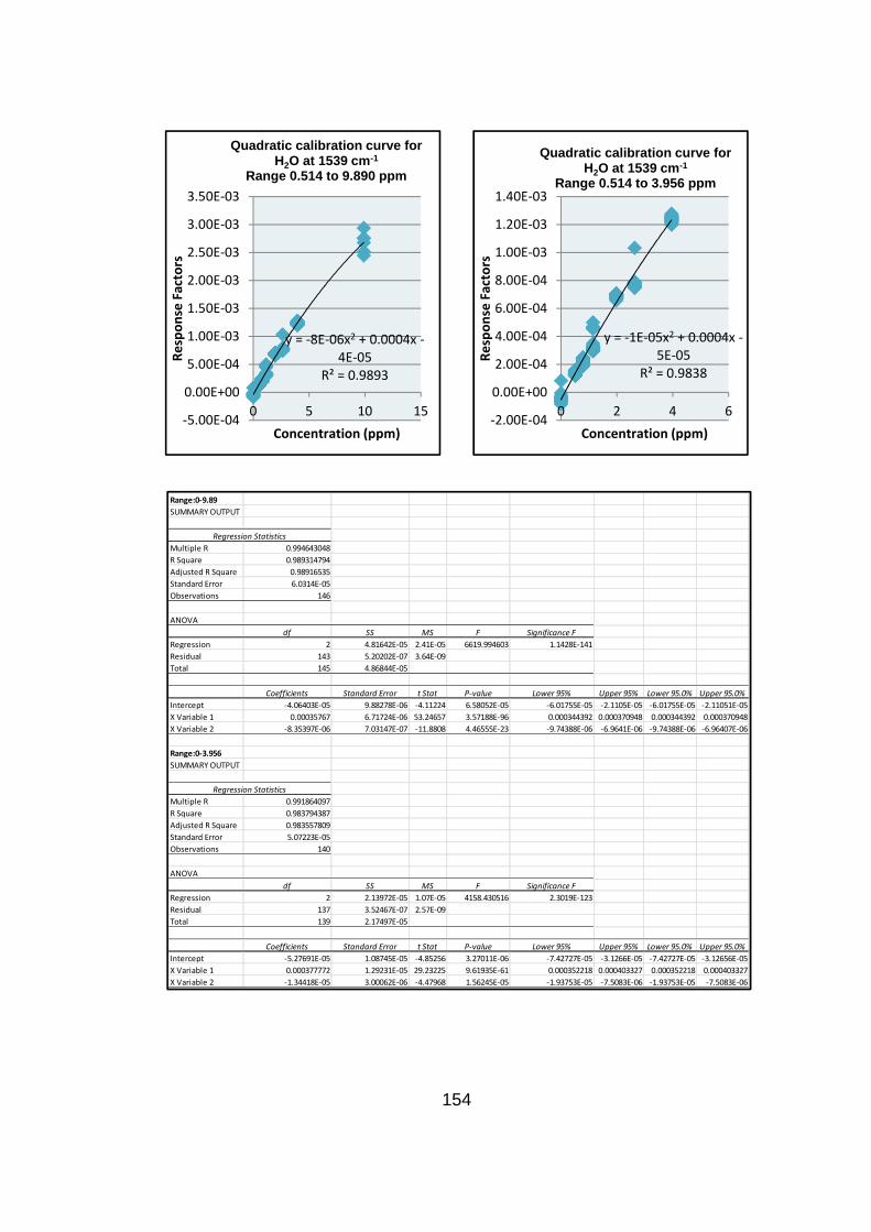
154

y = -8E-06x2 + 0.0004x -4E-05

R² = 0.9893

-5.00E-04

0.00E+00

5.00E-04

1.00E-03

1.50E-03

2.00E-03

2.50E-03

3.00E-03

3.50E-03

0 5 10 15

Resp

onse

Fac

tors

Concentration (ppm)



y = -1E-05x2 + 0.0004x -5E-05

R² = 0.9838

-2.00E-04

0.00E+00

2.00E-04

4.00E-04

6.00E-04

8.00E-04

1.00E-03

1.20E-03

1.40E-03

0 2 4 6

Resp

onse

Fac

tors

Concentration (ppm)













155

y = 0.0003x + 3E-05R² = 0.9681

-5.00E-04

0.00E+00

5.00E-04

1.00E-03

1.50E-03

2.00E-03

2.50E-03

3.00E-03

3.50E-03

4.00E-03

0 10 20

Resp

onse

Fac

tors

Concentration (ppm)



y = 0.0004x - 5E-05R² = 0.9822

-4.00E-04-2.00E-040.00E+002.00E-044.00E-046.00E-048.00E-041.00E-031.20E-031.40E-031.60E-031.80E-03

0 2 4 6

Resp

onse

Fac

tors

Concentration (ppm)



Range:0-9.89 LOQ 0.446466473SUMMARY OUTPUT

Regression StatisticsMultiple R 0.983936522R Square 0.96813108Adjusted R Square 0.967909768Standard Error 0.000129989Observations 146








Coefficients Standard Error t Stat P-value Lower 95% Upper 95% Lower 95.0% Upper 95.0%Intercept -5.14466E-05 9.3414E-06 -5.50737156 1.74121E-07 -6.99185E-05 -6.99185E-05 -3.29746E-05X Variable 1 0.000394745 4.54025E-06 86.94340076 9.8228E-122 0.000385767 0.000403723 0.000385767 0.000403723

156

y = -1E-05x2 + 0.0004x -8E-05

R² = 0.9818

-5.00E-04

0.00E+00

5.00E-04

1.00E-03

1.50E-03

2.00E-03

2.50E-03

3.00E-03

3.50E-03

4.00E-03

0 5 10 15

Resp

onse

Fac

tors

Concentration (ppm)



y = -2E-05x2 + 0.0005x - 1E-04

R² = 0.9848

-4.00E-04-2.00E-040.00E+002.00E-044.00E-046.00E-048.00E-041.00E-031.20E-031.40E-031.60E-031.80E-03

0 2 4 6

Resp

onse

Fac

tors

Concentration (ppm)







Coefficients Standard Error t Stat P-value Lower 95% Upper 95% Lower 95.0% Upper 95.0%Intercept -8.40021E-05 1.62095E-05 -5.18227 7.32946E-07 -0.000116043 -5.1961E-05 -0.000116043 -5.19609E-05X Variable 1 0.000443988 1.10499E-05 40.18033 8.68789E-80 0.000422146 0.00046583 0.000422146 0.00046583X Variable 2 -1.16971E-05 1.1317E-06 -10.3359 4.7751E-19 -1.39341E-05 -9.4601E-06 -1.39341E-05 -9.46005E-06





Coefficients Standard Error t Stat P-value Lower 95% Upper 95% Lower 95.0% Upper 95.0%Intercept -9.67657E-05 1.27957E-05 -7.56235 5.31E-12 -0.00012207 -7.1461E-05 -0.00012207 -7.14614E-05X Variable 1 0.000465223 1.52342E-05 30.53816 9.66624E-63 0.000435097 0.000495349 0.000435097 0.000495349X Variable 2 -1.71046E-05 3.55311E-06 -4.81397 3.88367E-06 -2.4131E-05 -1.0078E-05 -2.4131E-05 -1.00781E-05

157

y = 3E-05x + 0.0003R² = 0.9952

0

0.002

0.004

0.006

0.008

0 50 100 150 200 250 300

Resp

onse

fact

ors

Concentration (ppm)



Regression StatisticsMultiple R 0.993773918R Square 0.9875866Adjusted R Square0.98737971Standard Error0.000300009Observations 62


Regression 1 0.000429639 0.000429639 4773.486496 6.76708E-59Residual 60 5.40031E-06 9.00052E-08Total 61 0.000435039

Coefficients Standard Error t Stat P-value Lower 95% Upper 95% Lower 95.0% Upper 95.0%Intercept 0.000541173 5.7874E-05 9.350877632 2.55E-13 0.000425408 0.000656938 0.000425408 0.000657X Variable 1 2.24595E-05 3.25075E-07 69.09042261 6.76708E-59 2.18093E-05 2.31098E-05 2.18093E-05 2.31E-05




Regression 1 0.000218282 0.000218282 6.47881E-62Residual 52 1.0581E-06 2.03481E-08Total 53 0.00021934


APPENDIX 3:

Linear and Quadratic Calibration Data for all C2H2 wavenumbers:

Standard 1: Low range linear data for C2H2 at 3313/3266 cm-1

158

Standard 1: Low range quadratic data for C2H2 at 3313/3266 cm-1

y = -2E-08x2 + 3E-05x + 0.0002R² = 0.9973

00.0010.0020.0030.0040.0050.0060.007

0 50 100 150 200 250 300

Resp

onse

fact

ors

Concentration (ppm)






Coefficients Standard Error t Stat P-value Lower 95% Upper 95% Lower 95.0% Upper 95.0%Intercept 0.000119442 3.02044E-05 3.954469892 0.000208073 5.90035E-05 0.000179881 5.90035E-05 0.00018X Variable 1 3.11699E-05 4.59114E-07 67.89139454 1.04101E-57 3.02512E-05 3.20886E-05 3.02512E-05 3.21E-05X Variable 2 -2.35213E-08 1.19715E-09 -19.64766375 1.43584E-27 -2.59168E-08 -2.11258E-08 -2.59168E-08 -2.1E-08





Coefficients Standard Error t Stat P-value Lower 95% Upper 95% Lower 95.0% Upper 95.0%Intercept 0.000165768 3.50422E-05 4.730525481 1.81124E-05 9.54179E-05 0.000236118 9.54179E-05 0.000236X Variable 1 2.97686E-05 7.32934E-07 40.61569695 1.63999E-40 2.82972E-05 3.12401E-05 2.82972E-05 3.12E-05X Variable 2 -1.75965E-08 2.72201E-09 -6.464520777 3.81502E-08 -2.30612E-08 -1.21318E-08 -2.30612E-08 -1.2E-08

159

y = 6E-05x - 0.0001R² = 0.9991

-0.005

0

0.005

0.01

0.015

0.02

0 50 100 150 200 250 300

Resp

onse

fact

ors

Concentration (ppm)


C2H2





Coefficients Standard Error t Stat P-value Lower 95% Upper 95% Lower 95.0% Upper 95.0%Intercept 0.000137034 7.89304E-05 1.736136429 0.087672483 -2.08504E-05 0.000294918 -2.08504E-05 0.000295X Variable 1 5.81187E-05 4.43347E-07 131.09075 1.80548E-75 5.72318E-05 5.90055E-05 5.72318E-05 5.9E-05





Coefficients Standard Error t Stat P-value Lower 95% Upper 95% Lower 95.0% Upper 95.0%Intercept -0.000148709 3.2472E-05 -4.579608482 2.94031E-05 -0.000213869 -8.35493E-05 -0.000213869 -8.4E-05X Variable 1 6.19003E-05 2.55013E-07 242.7342983 4.18159E-81 6.13886E-05 6.2412E-05 6.13886E-05 6.24E-05

Standard 1: Low range linear data for C2H2 at 1305 cm-1

160

Standard 1: Low range quadratic data for C2H2 at 1305 cm-1

y = 2E-08x2 + 6E-05x + 6E-05R² = 0.9997

-0.005

0

0.005

0.01

0.015

0.02

0 50 100 150 200 250 300

Resp

onse

fact

ors

Concentration (ppm)






Coefficients Standard Error t Stat P-value Lower 95% Upper 95% Lower 95.0% Upper 95.0%Intercept -0.000299416 8.00414E-05 -3.740765936 0.000417336 -0.000459578 -0.000139254 -0.000459578 -0.00014X Variable 1 6.7133E-05 1.21665E-06 55.17869324 1.77188E-52 6.46985E-05 6.95675E-05 6.46985E-05 6.96E-05X Variable 2 -2.43422E-08 3.17245E-09 -7.673013107 1.95761E-10 -3.06903E-08 -1.79942E-08 -3.06903E-08 -1.8E-08


Regression StatisticsMultiple R 0.99983002R Square 0.999660068Adjusted R Square0.999646738Standard Error9.38139E-05Observations 54



Coefficients Standard Error t Stat P-value Lower 95% Upper 95% Lower 95.0% Upper 95.0%Intercept 5.95021E-05 3.07854E-05 1.932801297 0.058822628 -2.30221E-06 0.000121307 -2.30221E-06 0.000121X Variable 1 5.62766E-05 6.439E-07 87.3994687 3.16092E-57 5.49839E-05 5.75692E-05 5.49839E-05 5.76E-05X Variable 2 2.15611E-08 2.39136E-09 9.016255578 3.89607E-12 1.67602E-08 2.63619E-08 1.67602E-08 2.64E-08

161

y = 1E-05x + 0.0003R² = 0.9953

00.0020.0040.0060.008

0.010.012

0.000 200.000 400.000 600.000 800.000 1000.000

Resp

onse

fact

ors

Concentration (ppm)


C2H2

Standard 2: Low range linear data for C2H2 at 3313/3266 cm-1





Coefficients Standard Error t Stat P-value Lower 95% Upper 95% Lower 95.0% Upper 95.0%Intercept 0.001105505 0.000110851 9.972908057 4.47E-15 0.00088442 0.001326591 0.00088442 0.001327X Variable 1 1.14859E-05 1.12529E-07 102.0709525 6.80372E-78 1.12615E-05 1.17104E-05 1.12615E-05 1.17E-05






162

y = -2E-09x2 + 2E-05x - 7E-06R² = 0.9989

-0.005

0

0.005

0.01

0.015

0.02

0 200 400 600 800 1000 1200 1400

Resp

onse

fact

ors

Concentration (ppm)






Coefficients Standard Error t Stat P-value Lower 95% Upper 95% Lower 95.0% Upper 95.0%Intercept 0.000319925 8.05641E-05 3.971055945 0.000173226 0.000159204 0.000480646 0.000159204 0.000481X Variable 1 1.4077E-05 1.95537E-07 71.99126204 1.18457E-66 1.36869E-05 1.44671E-05 1.36869E-05 1.45E-05X Variable 2 -9.95937E-10 7.17525E-11 -13.88015888 1.18488E-21 -1.13908E-09 -8.52794E-10 -1.13908E-09 -8.5E-10





Coefficients Standard Error t Stat P-value Lower 95% Upper 95% Lower 95.0% Upper 95.0%Intercept -6.58446E-06 5.12899E-05 -0.128377245 0.898259377 -0.000109079 9.59103E-05 -0.000109079 9.59E-05X Variable 1 1.58585E-05 2.02329E-07 78.37962879 1.61266E-64 1.54541E-05 1.62628E-05 1.54541E-05 1.63E-05X Variable 2 -2.38214E-09 1.42987E-10 -16.65984766 9.09852E-25 -2.66788E-09 -2.09641E-09 -2.66788E-09 -2.1E-09


163

y = 4E-06x + 0.0001R² = 0.9975

-0.002

0

0.002

0.004

0.006

0.008

0 200 400 600 800 1000 1200 1400

Resp

onse

fact

ors

Concentration (ppm)


C2H2











Coefficients Standard Error t Stat P-value Lower 95% Upper 95% Lower 95.0% Upper 95.0%Intercept 0.000119346 1.74567E-05 6.836717215 3.84532E-09 8.4462E-05 0.000154231 8.4462E-05 0.000154X Variable 1 4.31355E-06 2.725E-08 158.2950251 1.20E-83 4.25909E-06 4.368E-06 4.25909E-06 4.37E-06

164

y = -5E-10x2 + 5E-06x - 5E-06R² = 0.9991

-0.002

0

0.002

0.004

0.006

0.008

0 200 400 600 800 1000 1200 1400

Resp

onse

fact

ors

Concentration (ppm)


C2H2






Coefficients Standard Error t Stat P-value Lower 95% Upper 95% Lower 95.0% Upper 95.0%Intercept 4.68541E-05 2.33658E-05 2.005244339 0.048919132 2.2841E-07 9.34798E-05 2.2841E-07 9.34798E-05X Variable 1 4.66101E-06 5.6369E-08 82.68742775 5.7473E-70 4.54853E-06 4.77349E-06 4.54853E-06 4.77349E-06X Variable 2 -2.41568E-10 2.06631E-11 -11.69078217 6.27893E-18 -2.828E-10 -2.00335E-10 -2.828E-10 -2.00335E-10


Regression StatisticsMultiple R 0.999546136R Square 0.999092478Adjusted R Square0.999063204Standard Error 5.3725E-05Observations 65


Regression 2 0.000197012 9.8506E-05 34127.96725 4.93817E-95Residual 62 1.78955E-07 2.88637E-09Total 64 0.000197191

Coefficients Standard Error t Stat P-value Lower 95% Upper 95% Lower 95.0% Upper 95.0%Intercept -5.03718E-06 1.59233E-05 -0.316340058 0.752807008 -3.68674E-05 2.67931E-05 -3.68674E-05 2.67931E-05X Variable 1 4.94463E-06 6.25749E-08 79.01936911 5.99392E-64 4.81954E-06 5.06972E-06 4.81954E-06 5.06972E-06X Variable 2 -4.62334E-10 4.42154E-11 -10.45641528 2.58555E-15 -5.50719E-10 -3.73949E-10 -5.50719E-10 -3.73949E-10

165

y = 4E-06x + 0.0001R² = 0.9978

-0.002

0

0.002

0.004

0.006

0.008

0 200 400 600 800 1000 1200 1400

Resp

onse

fact

ors

Concentration (ppm)


C2H2








Regression StatisticsMultiple R 0.998913998R Square 0.997829175Adjusted R Square0.997794718Standard Error 8.3611E-05Observations 65



Coefficients Standard Error t Stat P-value Lower 95% Upper 95% Lower 95.0% Upper 95.0%Intercept 0.000104041 1.64741E-05 6.315445483 3.06535E-08 7.11203E-05 0.000136962 7.11203E-05 0.000137X Variable 1 4.37615E-06 2.57161E-08 170.1711666 1.27258E-85 4.32476E-06 4.42754E-06 4.32476E-06 4.43E-06

166

y = -4E-10x2 + 5E-06x - 5E-06R² = 0.999

-0.002

0

0.002

0.004

0.006

0.008

0 200 400 600 800 1000 1200 1400

Resp

onse

fact

ors

Concentration (ppm)


C2H2






Coefficients Standard Error t Stat P-value Lower 95% Upper 95% Lower 95.0% Upper 95.0%Intercept 4.16488E-05 2.72298E-05 1.529532093 0.130771472 -1.26874E-05 9.59851E-05 -1.26874E-05 9.6E-05X Variable 1 4.67449E-06 6.56899E-08 71.15991139 1.39068E-65 4.54341E-06 4.80557E-06 4.54341E-06 4.81E-06X Variable 2 -2.06942E-10 2.40799E-11 -8.593964518 1.8312E-12 -2.54992E-10 -1.58891E-10 -2.54992E-10 -1.6E-10





Coefficients Standard Error t Stat P-value Lower 95% Upper 95% Lower 95.0% Upper 95.0%Intercept -4.83448E-06 1.67756E-05 -0.28818597 0.774165614 -3.83683E-05 2.86994E-05 -3.83683E-05 2.87E-05X Variable 1 4.92856E-06 6.59246E-08 74.76050061 1.79579E-62 4.79678E-06 5.06034E-06 4.79678E-06 5.06E-06X Variable 2 -4.04709E-10 4.65835E-11 -8.68780861 2.55682E-12 -4.97828E-10 -3.1159E-10 -4.97828E-10 -3.1E-10

167

y = 0.0091x + 0.1526R² = 0.9933

0123456

0 100 200 300 400 500 600

Resp

onse

fact

ors

Concentration (ppm)


C2H2

Standard 2: Low range linear data for C2H2 at 3313/3266 cm-1 with internal

standard




Regression 1 185.1591831 185.1591831 11463.62576 5.19447E-82Residual 73 1.179087721 0.016151887Total 74 186.3382709

Coefficients Standard Error t Stat P-value Lower 95% Upper 95% Lower 95.0% Upper 95.0%Intercept 0.196101358 0.033390231 5.873015879 1.17521E-07 0.129554723 0.262647993 0.129554723 0.262648X Variable 1 0.00889412 8.30696E-05 107.0683229 5.19447E-82 0.008728562 0.009059677 0.008728562 0.00906






168

y = -4E-06x2 + 0.0113x - 0.0073R² = 0.9998

-10123456

0 100 200 300 400 500 600

Resp

onse

fact

ors

Concentration (ppm)


C2H2

Standard 2: Low range quadratic data for C2H2 at 3313/3266 cm-1 with

internal standard





Coefficients Standard Error t Stat P-value Lower 95% Upper 95% Lower 95.0% Upper 95.0%Intercept 0.004388551 0.012585948 0.348686525 0.728342244 -0.020701079 0.02947818 -0.020701079 0.029478X Variable 1 0.010920093 8.08512E-05 135.064149 2.37736E-88 0.010758919 0.011081267 0.010758919 0.011081X Variable 2 -3.34083E-06 1.26474E-07 -26.41513549 8.86497E-39 -3.59295E-06 -3.0887E-06 -3.59295E-06 -3.1E-06





Coefficients Standard Error t Stat P-value Lower 95% Upper 95% Lower 95.0% Upper 95.0%Intercept -0.007291936 0.007125124 -1.023411827 0.310089809 -0.021534856 0.006950984 -0.021534856 0.006951X Variable 1 0.011255369 5.24605E-05 214.549467 9.89911E-91 0.011150502 0.011360236 0.011150502 0.01136X Variable 2 -4.14067E-06 9.47549E-08 -43.6987218 2.72658E-48 -4.33008E-06 -3.95126E-06 -4.33008E-06 -4E-06

169

y = 0.0026x + 0.0315R² = 0.9955

0

0.5

1

1.5

0 100 200 300 400 500 600

Resp

onse

fact

ors

Concentration (ppm)

Linear calibration curve for C2H2 at 1350 cm-1:Range 194.137 to 535. 189 ppm

C2H2

Standard 2: Low range linear data for C2H2 at 1350 cm-1 with internal

standard










Coefficients Standard Error t Stat P-value Lower 95% Upper 95% Lower 95.0% Upper 95.0%Intercept 0.029247675 0.007609179 3.843735871 0.000281237 0.014046592 0.044448757 0.014046592 0.044449X Variable 1 0.002562368 2.11286E-05 121.2750964 2.36646E-77 0.002520158 0.002604577 0.002520158 0.002605

170

y = -9E-07x2 + 0.003x - 0.0037R² = 0.9997

-0.5

0

0.5

1

1.5

0 100 200 300 400 500 600Resp

onse

fact

ors

Concentration (ppm)

Quadratic calibration curve for C2H2 at 1350cm-1:Range 194.137 to 535.189 ppm

C2H2

Standard 2: Low range quadratic data for C2H2 at 1350 cm-1 with internal

standard





Coefficients Standard Error t Stat P-value Lower 95% Upper 95% Lower 95.0% Upper 95.0%Intercept -0.001199806 0.003524426 -0.340425946 0.734513489 -0.008223977 0.005824365 -0.008223977 0.005824365X Variable 1 0.002957084 2.30959E-05 128.0348657 1.1902E-87 0.002911054 0.003003114 0.002911054 0.003003114X Variable 2 -7.23268E-07 3.66183E-08 -19.7515645 5.22739E-31 -7.96248E-07 -6.50288E-07 -7.96248E-07 -6.50288E-07


Regression StatisticsMultiple R 0.999811388R Square 0.999622812Adjusted R Square0.999610838Standard Error 0.0084423Observations 66


Regression 2 11.89983468 5.949917339 83481.32631 1.4506E-108Residual 63 0.004490163 7.12724E-05Total 65 11.90432484


171

y = 0.0041x + 0.1161R² = 0.9848

0

0.5

1

1.5

2

2.5

0 100 200 300 400 500 600

Resp

onse

fact

ors

Concentration (ppm)

Linear calibration curve for C2H2 at 1305cm-1:Range 194.137 to 535.189 ppm

C2H2


standard











172

y = -3E-06x2 + 0.0056x + 0.0035R² = 0.9998

0

0.5

1

1.5

2

2.5

0 100 200 300 400 500 600

Resp

onse

fact

ors

Concentration (ppm)

Quadratic calibration curve for C2H2 at 1305cm-1:Range 194.137to 535.189 ppm

C2H2


standard











173

y = 0.0001x + 0.0014R² = 0.9879

-0.01

0

0.01

0.02

0.03

0.04

0 50 100 150 200 250 300

Resp

onse

fact

ors

Concentration (ppm)

Linear calibration curve for C2H2 at 3313/3266 cm-1:Range 94.804 to 261.35 5ppm

C2H2

Standard 3: Low range linear data for C2H2 at 3313/3266/ cm-1











174

y = -1E-07x2 + 0.0002x - 0.0002R² = 0.9941

-0.01

0

0.01

0.02

0.03

0.04

0 50 100 150 200 250 300

Resp

onse

fact

ors

Concentration (ppm)

Quadratic calibration curve for C2H2 at 3313/3266 cm-1:Range 94.804to 261.350 ppm

C2H2












175

y = 5E-05x + 0.0005R² = 0.9856

-0.005

0

0.005

0.01

0.015

0 50 100 150 200 250 300Resp

onse

fact

ors

Concentration (ppm)

Linear calibration curve for C2H2 at 1350 cm-1:Range 94.804to 291.265 ppm

C2H2












176

y = -5E-08x2 + 6E-05x - 0.0001R² = 0.9938

-0.005

0

0.005

0.01

0.015

0 50 100 150 200 250 300Resp

onse

fact

ors

Concentration (ppm)


C2H2






Coefficients Standard Error t Stat P-value Lower 95% Upper 95% Lower 95.0% Upper 95.0%Intercept -7.82532E-05 0.00010815 -0.723561266 0.471746201 -0.000293952 0.000137445 -0.000293952 0.000137X Variable 1 5.85184E-05 1.35324E-06 43.24304126 3.09938E-52 5.58194E-05 6.12174E-05 5.58194E-05 6.12E-05X Variable 2 -4.48241E-08 4.11495E-09 -10.8929974 1.01132E-16 -5.30311E-08 -3.66171E-08 -5.30311E-08 -3.7E-08





Coefficients Standard Error t Stat P-value Lower 95% Upper 95% Lower 95.0% Upper 95.0%Intercept -0.000108363 0.000113765 -0.952513824 0.344595642 -0.00033585 0.000119124 -0.00033585 0.000119X Variable 1 5.95484E-05 1.60674E-06 37.06170789 1.54586E-43 5.63356E-05 6.27613E-05 5.63356E-05 6.28E-05X Variable 2 -4.93176E-08 5.49026E-09 -8.982742916 9.15023E-13 -6.0296E-08 -3.83391E-08 -6.0296E-08 -3.8E-08

177

y = 5E-05x + 0.0006R² = 0.986

0

0.005

0.01

0.015

0 50 100 150 200 250 300

Resp

onse

fact

ors

Concentration (ppm)


C2H2












178

y = -5E-08x2 + 6E-05x - 8E-05R² = 0.9942

-0.005

0

0.005

0.01

0.015

0 50 100 150 200 250 300Resp

onse

fact

ors

Concentration (ppm)


C2H2








Regression StatisticsMultiple R 0.997072979R Square 0.994154526Adjusted R Square0.993962871Standard Error 0.00025705Observations 64




179

y = 0.002x + 0.0129R² = 0.9913

0

0.1

0.2

0.3

0.4

0.5

0 50 100 150 200 250

Resp

onse

fact

ors

Concentration (ppm)


C2H2

Standard 3: Low range linear data for C2H2 at 3313/3266 cm-1 with internal

standard











180

y = -2E-06x2 + 0.0025x + 0.0008R² = 0.9952

0

0.1

0.2

0.3

0.4

0.5

0 50 100 150 200 250

Resp

onse

fact

ors

Concentration (ppm)

Quadratic calibration curve for C2H2 at 3313/3266 cm-1:Range 56.691to 230.238 ppm

C2H2

Standard 3: Low range quadratic data for C2H2 at 3313/3266 cm-1 with

internal standard





Coefficients Standard Error t Stat P-value Lower 95% Upper 95% Lower 95.0% Upper 95.0%Intercept 0.002738763 0.003469311 0.789425523 0.432824423 -0.004194103 0.009671629 -0.004194103 0.009672X Variable 1 0.002383721 6.98155E-05 34.14313573 2.35885E-42 0.002244205 0.002523236 0.002244205 0.002523X Variable 2 -1.60036E-06 2.91484E-07 -5.490372449 7.64412E-07 -2.18284E-06 -1.01787E-06 -2.18284E-06 -1E-06






181

y = 0.0007x - 0.0023R² = 0.9916

-0.05

0

0.05

0.1

0.15

0 50 100 150 200 250Resp

onse

fact

ors

Concentration (ppm)


C2H2


standard





Coefficients Standard Error t Stat P-value Lower 95% Upper 95% Lower 95.0% Upper 95.0%Intercept -0.002611383 0.001077378 -2.423831865 0.018194373 -0.004763693 -0.000459073 -0.004763693 -0.00046X Variable 1 0.000660223 7.00161E-06 94.2958514 2.13415E-70 0.000646235 0.00067421 0.000646235 0.000674





Coefficients Standard Error t Stat P-value Lower 95% Upper 95% Lower 95.0% Upper 95.0%Intercept -0.002286511 0.001121496 -2.038803182 0.046287699 -0.00453404 -3.89814E-05 -0.00453404 -3.9E-05X Variable 1 0.000655572 8.12627E-06 80.67319116 8.34E-59 0.000639286 0.000671857 0.000639286 0.000672

182

y = 1E-07x2 + 0.0006x - 0.0016R² = 0.9917

-0.05

0

0.05

0.1

0.15

0 50 100 150 200 250Resp

onse

fact

ors

Concentration (ppm)


C2H2


standard





Coefficients Standard Error t Stat P-value Lower 95% Upper 95% Lower 95.0% Upper 95.0%Intercept -0.001652326 0.001388153 -1.190305055 0.238464267 -0.004427204 0.001122553 -0.004427204 0.001122553X Variable 1 0.000625632 2.73799E-05 22.85005442 6.76113E-32 0.000570901 0.000680364 0.000570901 0.000680364X Variable 2 1.51997E-07 1.13161E-07 1.343191383 0.184106234 -7.42089E-08 3.78203E-07 -7.42089E-08 3.78203E-07





Coefficients Standard Error t Stat P-value Lower 95% Upper 95% Lower 95.0% Upper 95.0%Intercept -0.001595868 0.001365887 -1.168374937 0.247787979 -0.004334306 0.00114257 -0.004334306 0.00114257X Variable 1 0.000628754 3.12349E-05 20.12985852 9.12358E-27 0.000566132 0.000691376 0.000566132 0.000691376X Variable 2 1.28566E-07 1.44565E-07 0.889326696 0.377772294 -1.6127E-07 4.18401E-07 -1.6127E-07 4.18401E-07

Documents

The development and evaluation of analytical methods for