Embed Size (px)
Citation preview
University of Pennsylvania University of Pennsylvania
ScholarlyCommons ScholarlyCommons
Publicly Accessible Penn Dissertations
2017
The Determinants And Implications Of Firms' Workforce The Determinants And Implications Of Firms' Workforce
Configuration: The Case Of Home Health Configuration: The Case Of Home Health
Kunhee Kim University of Pennsylvania, [email protected]
Follow this and additional works at: https://repository.upenn.edu/edissertations
Part of the Economics Commons, and the Health and Medical Administration Commons
Recommended Citation Recommended Citation Kim, Kunhee, "The Determinants And Implications Of Firms' Workforce Configuration: The Case Of Home Health" (2017). Publicly Accessible Penn Dissertations. 2393. https://repository.upenn.edu/edissertations/2393
This paper is posted at ScholarlyCommons. https://repository.upenn.edu/edissertations/2393 For more information, please contact [email protected].

The Determinants And Implications Of Firms' Workforce Configuration: The Case The Determinants And Implications Of Firms' Workforce Configuration: The Case Of Home Health Of Home Health
Abstract Abstract A fundamental challenge for labor-intensive firms facing demand uncertainty is how to configure their workforce to improve quality and performance. This dissertation investigates determinants of firms' workforce configuration, with a focus on the mix of temporary and permanent nurses, and its implications on patient outcomes, a central measure of performance in health care. This is a timely topic since many industries including health care are increasingly using alternative work arrangements. This dissertation uses novel and rich proprietary data from a large US freestanding home health company. The data provide detailed information on both the consumption and production sides of home health care delivery: utilization, referral sources, risk factors and health outcomes of patients as well as nurses’ work logs and human resources characteristics. In Chapter 1, I investigate the effect of firms’ labor mix on patient readmission, a main quality marker in post-acute care, using exogenous variation in full-time nurses’ activeness in the patient’s neighborhood and unavailability of nearest full-time nurses. I find that patients who received one standard-deviation higher proportion of full-time nurse visits were 7 percent less likely to be readmitted. In Chapter 2, I investigate the effect of reputation on firms’ labor mix strategy under demand uncertainty. Firms face a trade-off in using temporary nurses: they provide flexibility in responding to demand fluctuations but may impede the establishment of reputation through lower quality of service. I present and test a model of firm’s labor mix choices where the labor mix dynamically shapes the market’s perception of the firm’s quality (i.e. reputation), and the firm’s demand is in turn stochastically linked to its reputation. I find evidence consistent with the model: firms with lower reputation, especially young firms, increased the percentage of full-time nurses with demand volatility. Young firms trade off short-term profitability for long-term reputation gains. In Chapter 3, I investigate the effect of firms’ workforce assignment on readmission through care discontinuity or handoffs. Using exogenous variation in workflow interruption caused by providers’ inactivity, I find handoffs to increase the likelihood of readmission. One in four readmissions during home health would be avoided if handoffs were eliminated.
Degree Type Degree Type Dissertation
Degree Name Degree Name Doctor of Philosophy (PhD)
Graduate Group Graduate Group Health Care Management & Economics
First Advisor First Advisor Guy David
Keywords Keywords Alternative work arrangements, Continuity of care, Hospital readmission, Organization of health care labor, Post-acute care, Workforce strategy under demand uncertainty
Subject Categories Subject Categories Economics | Health and Medical Administration
This dissertation is available at ScholarlyCommons: https://repository.upenn.edu/edissertations/2393
THE DETERMINANTS AND IMPLICATIONS OF FIRMS’ WORKFORCE
CONFIGURATION: THE CASE OF HOME HEALTH
Kunhee Kim
A DISSERTATION
in
Health Care Management
For the Graduate Group in Managerial Science and Applied Economics
Presented to the Faculties of the University of Pennsylvania
in
Partial Fulfillment of the Requirements for the
Degree of Doctor of Philosophy
2017
Supervisor of Dissertation
Guy David, Gilbert and Shelley Harrison Associate Professor of Health Care Management
Graduate Group Chairperson
Catherine Schrand, Celia Z. Moh Professor, Professor of Accounting
Dissertation Committee:
Mark Pauly, Bendheim Professor, Professor of Health Care Management
Scott Harrington, Alan B. Miller Professor, Professor of Health Care Management, andProfessor of Insurance and Risk Management
Peter Cappelli, George W. Taylor Professor, Professor of Management

THE DETERMINANTS AND IMPLICATIONS OF FIRMS’ WORKFORCE
CONFIGURATION: THE CASE OF HOME HEALTH
c© COPYRIGHT
2017
Kunhee Kim
This work is licensed under the
Creative Commons Attribution
NonCommercial-ShareAlike 3.0
License
To view a copy of this license, visit
http://creativecommons.org/licenses/by-nc-sa/3.0/

Dedicated to my father Hyungbyung
iii

ACKNOWLEDGEMENT
I feel honored to have learned from wonderful mentors and colleagues in a great institution
with abundant resources. During my five years of graduate school, I learned a lot both as an
academic and as a human being. A life-changing event happened to me, which influenced
me quite deeply, and I am very grateful for many people who served as an anchor so I
could walk on and grow. First, I am indebted to my advisor and mentor, Guy David.
Completing graduate school and this dissertation would not have been possible without his
mentoring, support and encouragement. I am amazed at how one great person can make
such a big positive impact. I aspire to emulate him and pay forward his generous help.
A lot of challenges have been made easier and enjoyable by working with him. Second, I
am also indebted to my dissertation committee members, Mark Pauly, Scott Harrington,
and Peter Cappelli. I still remember how much I learned from just one email response
from Mark after I sent him an early draft for a dissertation even before he signed on to
be on the committee. After each meeting with him, I was enlightened with new insights
and an expanded field of vision. Scott provided sharp and invaluable comments rooted
in the institutional knowledge or econometrics. I am especially grateful for his agreeing
to be on the committee and providing tremendous support during my job search. My
research also greatly benefitted from Peter’s insightful comments and expert knowledge in
the human resources management field. I am indebted to his support for my navigation in
the management field.
I am grateful to numerous people in the Wharton School and the Leonard Davis Institute of
Health Economics (LDI). I thank Lynn Selhat for having many enlightening conversations
about how to write research papers. I thank Ashley Swanson and Jon Kolstad, from whom
I learned a lot about empirical research, Joanne Levy, who provided generous support and
cheerful encouragement, and Dan Polsky, who did not hesitate to give support in any ways
he could. I also thank Safa Brown, Megan Pellegrino, and Janice Singleton, and particularly,
Jennifer Gray and Tina Horowitz, who provided enormous help during my job search. I
iv

gratefully acknowledge financial support from the LDI.
I am also indebted to David Baiada, Alan Wright, Ann Gallagher, and Stephanie Finnel
for tremendous insight and data support. Without their support and willingness to take
the time to teach me about their institution, I would not have been able to complete my
dissertation.
I also thank my colleagues, Elena Andreyeva, Nora Becker, Amy Bond, Julius Chen, Vicki
Chen, Shulamite Chiu, Emma Dean, Sunita Desai, Qing Gong, Charu Gupta, Jinsoo Han,
Jessica Kim-Gina, Ambar La Forgia, Byounghoon Lee, Adam Leive, Kyle Myers, Bill Pa-
jerowski, Lindsey Patterson, Ellie Prager, Preethi Rao, Will Wang, Shinjae Won and Xing-
tan Zhang. My special thanks go to Manvi Bhatnagar, Tanvi Rai, and Nishant Ravi whose
friendship and support were a key ingredient of my progress in graduate school.
I feel deep gratitude to my in-laws, Mary, Reinhold, Reeta, and Mike, for welcoming me
into their family and looking out for my happiness and success, and for always supporting
me with compassion and fondness. My very special thanks go to my husband, Markus.
The graduate school life was so much more joyful and enlightening thanks to him. His
unconditional love and support as well as bottomless confidence in my abilities have been
critical for going through this challenging journey. Lastly, I owe infinite thanks to my
parents, Misung and Hyungbyung, and brother, Gunwoo. They provided limitless affection,
trust and confidence in me. I know that my father would have been very proud of me.
Kunhee Kim
May 2017
v

ABSTRACT
THE DETERMINANTS AND IMPLICATIONS OF FIRMS’ WORKFORCE
CONFIGURATION: THE CASE OF HOME HEALTH
Kunhee Kim
Guy David
A fundamental challenge for labor-intensive firms facing demand uncertainty is how to con-
figure their workforce to improve quality and performance. This dissertation investigates
determinants of firms’ workforce configuration, with a focus on the mix of temporary and
permanent nurses, and its implications on patient outcomes, a central measure of perfor-
mance in health care. This is a timely topic since many industries including health care
are increasingly using alternative work arrangements. This dissertation uses novel and rich
proprietary data from a large US freestanding home health company. The data provide
detailed information on both the consumption and production sides of home health care
delivery: utilization, referral sources, risk factors and health outcomes of patients as well as
nurses’ work logs and human resources characteristics. In Chapter 1, I investigate the effect
of firms’ labor mix on patient readmission, a main quality marker in post-acute care, using
exogenous variation in full-time nurses’ activeness in the patient’s neighborhood and unavail-
ability of nearest full-time nurses. I find that patients who received one standard-deviation
higher proportion of full-time nurse visits were 7 percent less likely to be readmitted. In
Chapter 2, I investigate the effect of reputation on firms’ labor mix strategy under demand
uncertainty. Firms face a trade-off in using temporary nurses: they provide flexibility in re-
sponding to demand fluctuations but may impede the establishment of reputation through
lower quality of service. I present and test a model of firm’s labor mix choices where the la-
bor mix dynamically shapes the market’s perception of the firm’s quality (i.e. reputation),
and the firm’s demand is in turn stochastically linked to its reputation. I find evidence
consistent with the model: firms with lower reputation, especially young firms, increased
vi

the percentage of full-time nurses with demand volatility. Young firms trade off short-term
profitability for long-term reputation gains. In Chapter 3, I investigate the effect of firms’
workforce assignment on readmission through care discontinuity or handoffs. Using exoge-
nous variation in workflow interruption caused by providers’ inactivity, I find handoffs to
increase the likelihood of readmission. One in four readmissions during home health would
be avoided if handoffs were eliminated.
vii

TABLE OF CONTENTS
ACKNOWLEDGEMENT . . . . . . . . . . . . . . . . . . . . . . . . . . . . . . . . . iv
ABSTRACT . . . . . . . . . . . . . . . . . . . . . . . . . . . . . . . . . . . . . . . . vi
LIST OF TABLES . . . . . . . . . . . . . . . . . . . . . . . . . . . . . . . . . . . . . xi
LIST OF ILLUSTRATIONS . . . . . . . . . . . . . . . . . . . . . . . . . . . . . . . xii
CHAPTER 1 : The Effect of Firms’ Labor Mix on Quality of Care . . . . . . . . . 1
1.1 Introduction . . . . . . . . . . . . . . . . . . . . . . . . . . . . . . . . . . . . 1
1.2 Background . . . . . . . . . . . . . . . . . . . . . . . . . . . . . . . . . . . . 4
1.3 Data . . . . . . . . . . . . . . . . . . . . . . . . . . . . . . . . . . . . . . . . 8
1.4 Inference Problem . . . . . . . . . . . . . . . . . . . . . . . . . . . . . . . . 10
1.5 Empirical Strategy . . . . . . . . . . . . . . . . . . . . . . . . . . . . . . . . 12
1.6 Results . . . . . . . . . . . . . . . . . . . . . . . . . . . . . . . . . . . . . . . 17
1.7 Conclusion . . . . . . . . . . . . . . . . . . . . . . . . . . . . . . . . . . . . 19
CHAPTER 2 : The Effect of Reputation on Firms’ Labor Mix Strategy under De-
mand Uncertainty . . . . . . . . . . . . . . . . . . . . . . . . . . . . 28
2.1 Introduction . . . . . . . . . . . . . . . . . . . . . . . . . . . . . . . . . . . . 28
2.2 Background on Home Health Care . . . . . . . . . . . . . . . . . . . . . . . 32
2.3 Theory . . . . . . . . . . . . . . . . . . . . . . . . . . . . . . . . . . . . . . . 33
2.4 Data . . . . . . . . . . . . . . . . . . . . . . . . . . . . . . . . . . . . . . . . 42
2.5 Evolution of Firm’s Demand Volatility, Reputation and Labor Mix: Descrip-
tive Facts . . . . . . . . . . . . . . . . . . . . . . . . . . . . . . . . . . . . . 44
2.6 Empirical Analysis . . . . . . . . . . . . . . . . . . . . . . . . . . . . . . . . 48
2.7 Alternative Explanations and Robustness Checks . . . . . . . . . . . . . . . 54
viii

2.8 Conclusion . . . . . . . . . . . . . . . . . . . . . . . . . . . . . . . . . . . . 59
2.9 Appendix: Proofs . . . . . . . . . . . . . . . . . . . . . . . . . . . . . . . . . 72
CHAPTER 3 : The Effect of Workforce Assignment on Performance . . . . . . . . 75
3.1 Introduction . . . . . . . . . . . . . . . . . . . . . . . . . . . . . . . . . . . . 75
3.2 Data . . . . . . . . . . . . . . . . . . . . . . . . . . . . . . . . . . . . . . . . 81
3.3 Empirical Strategy . . . . . . . . . . . . . . . . . . . . . . . . . . . . . . . . 85
3.4 Results on the Effects of Handoffs on the Likelihood of Rehospitalization . . 93
3.5 Conclusion . . . . . . . . . . . . . . . . . . . . . . . . . . . . . . . . . . . . 96
3.6 Appendix . . . . . . . . . . . . . . . . . . . . . . . . . . . . . . . . . . . . . 110
APPENDIX . . . . . . . . . . . . . . . . . . . . . . . . . . . . . . . . . . . . . . . . . 119
BIBLIOGRAPHY . . . . . . . . . . . . . . . . . . . . . . . . . . . . . . . . . . . . . 121
ix
LIST OF TABLES
TABLE 1 : Labor Supply and Pay Characteristics of Nurses by Work Arrange-
ments . . . . . . . . . . . . . . . . . . . . . . . . . . . . . . . . . . 22
TABLE 2 : Patient Severity and the Proportion of Full-Time Nurse Visits . . . 23
TABLE 3 : Mean Proportion of Full-Time Nurse Visits by Full-Time Nurses’
Activeness in the Local Area at the Start of Care . . . . . . . . . . 24
TABLE 4 : Balance of Covariates in the Patient Sample . . . . . . . . . . . . . 25
TABLE 5 : IV First-Stage Results: Effect of Full-time Nurses’ Activeness on the
Proportion of Full-Time Nurse Visits . . . . . . . . . . . . . . . . . 26
TABLE 6 : Main Results: Effect of Proportion of Full-Time Nurse Visits on
Patient Readmission . . . . . . . . . . . . . . . . . . . . . . . . . . 27
TABLE 7 : Summary Statistics . . . . . . . . . . . . . . . . . . . . . . . . . . . 65
TABLE 8 : Effects of Reputation on Firms’ Labor Mix Responses to Demand
Volatility . . . . . . . . . . . . . . . . . . . . . . . . . . . . . . . . . 66
TABLE 9 : Effects of Reputation on Firms’ Labor Mix Responses to Demand
Volatility by Firm Age . . . . . . . . . . . . . . . . . . . . . . . . . 67
TABLE 10 : Effects of Reputation on Firms’ Labor Mix Responses to Demand
Volatility among Young Firms Aged 0–12 Months . . . . . . . . . . 68
TABLE 11 : Effects of Reputation on Firms’ Labor Mix Responses to Demand
Volatility by Firm Age and Firm Size . . . . . . . . . . . . . . . . . 69
TABLE 12 : Effects of Reputation on Firms’ Labor Mix Responses to Demand
Volatility among “Not New in Town” Firms . . . . . . . . . . . . . 70
TABLE 13 : Robustness Check with Market Condition Controls: Effects of Rep-
utation on Firms’ Labor Mix Responses to Demand Volatility . . . 71
TABLE 14 : Sample Summary Statistics for the Sample Period 2012–2015 . . . 103
x

TABLE 15 : Distribution of the Number of Unique Nurses in Each Episode . . . 105
TABLE 16 : Distribution of Patient-Day Observations and the Likelihood of Nurse
Handoff, Nurse Visit, and Readmission by the Availability of Nurse
Who Visited a Patient in the Last Visit . . . . . . . . . . . . . . . 106
TABLE 17 : OLS: Patients Experiencing a Handoff Are More Likely to Be Re-
hospitalized . . . . . . . . . . . . . . . . . . . . . . . . . . . . . . . 107
TABLE 18 : GMM 2SLS: Experiencing Handoffs Increases the Likelihood of Read-
mission . . . . . . . . . . . . . . . . . . . . . . . . . . . . . . . . . . 108
TABLE 19 : OLS: The Effects of Handoffs Varies by the Frequency and Sequenc-
ing of Handoffs . . . . . . . . . . . . . . . . . . . . . . . . . . . . . 109
TABLE 20 : OLS: Patients Experiencing a Handoff Are More Likely to Be Re-
hospitalized within 30 Days of Hospital Discharge . . . . . . . . . . 111
TABLE 21 : GMM 2SLS: Experiencing Handoffs Increases the Likelihood of Read-
mission within 30 Days of Hospital Discharge . . . . . . . . . . . . 112
TABLE 22 : Logit: Patients Experiencing a Handoff Are More Likely to Be Re-
hospitalized . . . . . . . . . . . . . . . . . . . . . . . . . . . . . . . 113
TABLE 23 : Key Measures of Patients’ Severity as Predictors of the Likelihood
of Readmission . . . . . . . . . . . . . . . . . . . . . . . . . . . . . 115
TABLE 24 : Distribution of Patient-Day Observations and the Likelihood of Nurse
Handoff, Nurse Visit, and Readmission by the Availability of Nurse
Who Visited a Patient in the Last Visit . . . . . . . . . . . . . . . 117
TABLE 25 : GMM 2SLS: Experiencing Handoffs Increases the Likelihood of Read-
mission . . . . . . . . . . . . . . . . . . . . . . . . . . . . . . . . . . 118
TABLE 26 : Summary Statistics on the Number of Workers in Each Home Health
Service Discipline . . . . . . . . . . . . . . . . . . . . . . . . . . . . 121
xi
LIST OF ILLUSTRATIONS
FIGURE 1 : Variation in the Proportion of Full-Time Nurse Visits across Pa-
tient Episodes . . . . . . . . . . . . . . . . . . . . . . . . . . . . . 21
FIGURE 2 : Measures of Reputation by Firm Age . . . . . . . . . . . . . . . . 61
FIGURE 3 : Demand Size and Volatility by Firm Age . . . . . . . . . . . . . . 62
FIGURE 4 : Labor Mix by Firm Age Bin . . . . . . . . . . . . . . . . . . . . . 63
FIGURE 5 : Relationship between Demand Volatility and Percentage of Full-
Time Nurses by Firm Age . . . . . . . . . . . . . . . . . . . . . . 64
FIGURE 6 : The Number of Ongoing Episodes and Readmissions by Home
Health Day . . . . . . . . . . . . . . . . . . . . . . . . . . . . . . . 97
FIGURE 7 : Fraction of Patient Episodes with at Least One, Two, Three, or
Four Handoffs by Home Health Day . . . . . . . . . . . . . . . . . 98
FIGURE 8 : Fraction of Patient-Days with Nurse Handoffs Conditional on Hav-
ing a Nurse Visit . . . . . . . . . . . . . . . . . . . . . . . . . . . 99
FIGURE 9 : Measures of Patient Severity Preceding the Nurse’s Inactivity . . 100
FIGURE 10 : Daily Workload of Nurses Preceding the Nurse’s Inactivity . . . . 101
FIGURE 11 : Daily Office Caseload Before and After the Nurse’s Inactivity . . 102
xii
CHAPTER 1 : The Effect of Firms’ Labor Mix on Quality of Care
1.1. Introduction
An increasing number of firms in the US hire workers in alternative work arrangements,
defined as temporary help agency, on-call, contract company, and independently contracted
or freelancing workers (Katz and Krueger, 2016). Between 2005 and 2015, the percentage of
workers in those arrangements rose from 10.7 percent to 15.8 percent, and 94 percent of the
net employment growth in the US economy during this period is estimated to have occurred
in alternative work arrangements (Katz and Krueger, 2016). Health care, in particular, is
one of the fastest growing industry groups with a 53-percent growth in the percentage
of health care professionals in alternative work arrangements between 2005 and 2015 and
a 74-percent growth between 1995 and 2015 (Katz and Krueger, 2016).1 This trend of
an increasing use of workers in alternative arrangements in health care naturally raises the
question of whether using more of these workers has any impact on patient health outcomes,
a central measure of performance in health care.
Key problems in estimating the impact of using alternative work arrangements on health
outcomes are attribution and selective assignment. A multitude of other organizational
factors, such as facility resources or technology tools, simultaneously influence the patient
experience and health outcomes. Provider organizations with more resources may adopt
staffing practices—such as hiring more professionals in permanent work arrangements or
providing better work environments—that achieve favorable health outcomes (Aiken et al.,
2007). Moreover, providers may selectively assign patients to professionals in different work
arrangements: for example, relatively healthier patients are matched with professionals in
alternative work arrangements.
1The percentage of health care professionals in alternative work arrangements was 5.3 percent, 6 percent,and 9.2 percent in 1995, 2005, and 2015, respectively. Health care professionals refers to workers in theHealthcare Practitioners and Technical Occupations and Healthcare Support Occupations groups, as definedby the Bureau of Labor Services. The former group includes physicians and nurses while the latter includesphysician aides and nurse aides.
1
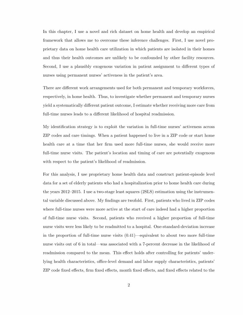
In this chapter, I use a novel and rich dataset on home health and develop an empirical
framework that allows me to overcome these inference challenges. First, I use novel pro-
prietary data on home health care utilization in which patients are isolated in their homes
and thus their health outcomes are unlikely to be confounded by other facility resources.
Second, I use a plausibly exogenous variation in patient assignment to different types of
nurses using permanent nurses’ activeness in the patient’s area.
There are different work arrangements used for both permanent and temporary workforces,
respectively, in home health. Thus, to investigate whether permanent and temporary nurses
yield a systematically different patient outcome, I estimate whether receiving more care from
full-time nurses leads to a different likelihood of hospital readmission.
My identification strategy is to exploit the variation in full-time nurses’ activeness across
ZIP codes and care timings. When a patient happened to live in a ZIP code or start home
health care at a time that her firm used more full-time nurses, she would receive more
full-time nurse visits. The patient’s location and timing of care are potentially exogenous
with respect to the patient’s likelihood of readmission.
For this analysis, I use proprietary home health data and construct patient-episode level
data for a set of elderly patients who had a hospitalization prior to home health care during
the years 2012–2015. I use a two-stage least squares (2SLS) estimation using the instrumen-
tal variable discussed above. My findings are twofold. First, patients who lived in ZIP codes
where full-time nurses were more active at the start of care indeed had a higher proportion
of full-time nurse visits. Second, patients who received a higher proportion of full-time
nurse visits were less likely to be readmitted to a hospital. One-standard-deviation increase
in the proportion of full-time nurse visits (0.41)—equivalent to about two more full-time
nurse visits out of 6 in total—was associated with a 7-percent decrease in the likelihood of
readmission compared to the mean. This effect holds after controlling for patients’ under-
lying health characteristics, office-level demand and labor supply characteristics, patients’
ZIP code fixed effects, firm fixed effects, month fixed effects, and fixed effects related to the
2
timings of the start and end of care. Moreover, this estimated effect is conservative since
when full-time nurses were active, firms tended to have sicker patients by several severity
measures.
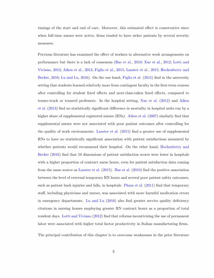
Previous literature has examined the effect of workers in alternative work arrangements on
performance but there is a lack of consensus (Bae et al., 2010; Xue et al., 2012; Lotti and
Viviano, 2012; Aiken et al., 2013; Figlio et al., 2015; Lasater et al., 2015; Hockenberry and
Becker, 2016; Lu and Lu, 2016). On the one hand, Figlio et al. (2015) find in the university
setting that students learned relatively more from contingent faculty in the first-term courses
after controlling for student fixed effects and next-class-taken fixed effects, compared to
tenure-track or tenured professors. In the hospital setting, Xue et al. (2012) and Aiken
et al. (2013) find no statistically significant difference in mortality in hospital units run by a
higher share of supplemental registered nurses (RNs). Aiken et al. (2007) similarly find that
supplemental nurses were not associated with poor patient outcomes after controlling for
the quality of work environments. Lasater et al. (2015) find a greater use of supplemental
RNs to have no statistically significant association with patient satisfactions measured by
whether patients would recommend their hospital. On the other hand, Hockenberry and
Becker (2016) find that 10 dimensions of patient satisfaction scores were lower in hospitals
with a higher proportion of contract nurse hours, even for patient satisfaction data coming
from the same source as Lasater et al. (2015). Bae et al. (2010) find the positive association
between the level of external temporary RN hours and several poor patient safety outcomes,
such as patient back injuries and falls, in hospitals. Pham et al. (2011) find that temporary
staff, including physicians and nurses, was associated with more harmful medication errors
in emergency departments. Lu and Lu (2016) also find greater service quality deficiency
citations in nursing homes employing greater RN contract hours as a proportion of total
resident days. Lotti and Viviano (2012) find that reforms incentivizing the use of permanent
labor were associated with higher total factor productivity in Italian manufacturing firms.
The principal contribution of this chapter is to overcome weaknesses in the prior literature
3
by accounting for the non-random matching of providers in different work arrangements with
patients. I demonstrate that accounting for this endogeneity is important as the OLS effects
of the proportion of full-time nurse visits are not statistically significant whereas the 2SLS
effects are statistically significant and greater in magnitude. To the best of my knowledge,
this chapter is the first to use an econometric method to overcome the inference problem.
Broadly, the chapter is related to the literature on the relationship between staffing and
quality (Needleman et al., 2011; Tong, 2011; Cook et al., 2012; Mark et al., 2013; Lin, 2014;
Matsudaira, 2014).
The remainder of this chapter is organized as follows. In Section 1.2, I provide brief back-
ground on home health care to provide necessary institutional details to understand my
empirical strategy. In Section 1.3, I describe the data and sample restriction rules. In Sec-
tion 1.4, I describe the key inference problems in estimating the effect of the proportion of
full-time nurse visits on patient readmission. In Section 1.5, I discuss the empirical strategy.
In Section 1.6, I present the estimation results. In Section 1.7, I conclude the chapter.
1.2. Background
Home health care, which is provided to homebound patients who need skilled nursing or
therapy services, is an important and rapidly growing segment of the post-acute care delivery
system. Home health care is composed of largely six service disciplines in which home health
firms demand labor: skilled nursing, home health or personal care aid, physical therapy,
speech-language pathology, occupational therapy, and medical social services.2 I provide a
detailed background on the home health care industry and the workforce distribution across
disciplines in Appendices A.1 and A.2, respectively, at the end of the dissertation.
In this chapter, I focus on the skilled nursing workforce—the combination of registered
nurses (RNs) and licensed practice nurses (LPNs)—since nurses provide the medical service
most relevant to potentially determining hospital readmissions and since their visits account
2Medicare covers only these six discipilnes.
4
for the majority of overall home health visits. Thus, among the six service disciplines, home
health firms’ demand for skilled nurses is the highest and they maintain the largest capacity
of them each week.
Nurses are hired under largely two compensation schemes: salary with guaranteed work and
expected number of visits for each week and piece-rate pays with no guaranteed work and
visit-based hiring. Thus, one can think of salaried nurses as “permanent” and piece-rate
paid as “temporary” workers in this chapter. Under salary, nurses can be hired either on
a full-time, part-time with benefits, or part-time without benefits basis, or for managerial
or administrative positions. Full-time nurses are the primary salaried work arrangement,
comprising 40 percent of a firm’s workforce every week on average. Under piece-rate pay,
nurses can be hired either on an on-call basis directly by the firms or hired as contractors
through temporary help agencies. On-call nurses are the primary piece-rate paid work
arrangement, comprising more than 30 percent of a firm’s workforce every week on average.
1.2.1. Differences between Permanent and Temporary nurses: Descriptive Statistics
A lack of consensus in the previous literature on the effect of alternative work arrange-
ments on quality and performance may reflect the fact that the effect plausibly varies
across settings. However, theoretically there are opposing directions through which workers
in alternative work arrangements can affect performance. On the one hand, lower-quality
workers may be more likely to sort into alternative work arrangements if firms have lower
standards of hiring for those arrangements. Once employed by a firm, workers hired in
alternative work arrangements may also have shorter engagement with the firm and lack
opportunities to develop firm-specific skills (Broschak and Davis-Blake, 2006; Cuyper et al.,
2008) or receive support from colleagues (Witte and Nswall, 2003). Negative worker out-
comes for workers in alternative work arrangements, such as lower wages or lower benefits,
could reduce their morale and productivity (Harley, 1994; Hockenberry and Becker, 2016).
On the other hand, using workers in alternative work arrangements could have a positive
5
effect on performance if they provide supplementary labor to address a shortage or high
workload of regular workers. Flexible staffing strategies could offset the negative effects of
low staffing or high workload per worker which have been consistently noted by previous
literature (Aiken et al., 2010; Kuntz et al., 2014; Berry Jaeker and Tucker, 2016). Moreover,
to the extent that alternative work arrangements are used as a screening device or stepping
stones for more permanent positions, the former do not necessarily attract less competent
nurses (Booth et al., 2002). However, this case is unlikely in in my data since it is rare
for permanent nurses to be hired first in temporary work arrangements and for temporary
nurses to change into permanent positions.
Before examining the effect of the proportion of full-time nurse visits on patient readmission,
I explore whether full-time nurses are different from nurses hired in other work arrangements.
If there is no meaningful difference, there is no reason for firms to differentially treat them
and expect any difference in the quality of care. In Table 1, I report mean values of key
labor supply and pay characteristics of nurses in each work arrangement. I focus on the
comparison of full-time and on-call nurses, who represent the majority of salaried and piece-
rate paid workforce.
Full-time nurses had substantially higher workloads, as measured in terms of number of
visits. Panel A shows that conditional on providing at least one visit, full-time nurses
provided 22 visits per week on average compared to on-call nurses who provided 9 visits per
week. However, the average length of visits provided by full-time nurses was at 46 minutes
shorter by 4 minutes than that of on-call nurses. Reflecting the difference in workloads, full-
time nurses were paid slightly less than 3 times the total weekly pay of on-call nurses, as
shown in Panel B. However, on the per-visit rate, full-time nurses get paid less than on-call
nurses by $12 on average, which may be a compensating differential for benefits. Moreover,
full-time nurses’ average length of employment of 21 months was 5 months longer than that
of on-call nurses.3
3To obtain these statistics, I restricted to nurses who terminated their employment, where the terminationwas defined as either permanently exiting the workforce or providing no visits for more than 90 consecutive
6
Another qualitative difference between salaried and piece-rate paid nurses lies in the amount
of training and attendance of case review conferences. Data on these aspects are unavailable.
However, according to interviews with administrators in the company which provided me
with the data, salaried nurses must receive training at the start of employment and get
additional training regularly. They also spend more time in the firm offices and attend
conferences with other care team members to review patient cases. On the other hand,
piece-rate paid nurses are not obliged to receive training at the start of employment and
do not typically receive additional training afterwards. They also do not usually attend
conferences for case reviews.
Table 1 alone cannot entirely explain why a higher proportion of full-time nurse visits would
improve patient outcome (i.e. reduce hospital readmission). However, data suggest that full-
time nurses accumulate much more experience by providing more visits as well as staying
employed for longer. To the extent that the experience has a positive correlation with
performance—whether it is due to the vintage effect or selection (Murnane and Phillips,
1981) or learning by doing (David and Brachet, 2009)—full-time nurses may provide higher
quality of care.4 The same effect is predicted to the extent that full-time nurses develop
greater expertise and superior knowledge of firms’ culture and standards by spending more
time at firms’ offices and with colleagues. These forces, however, might be counterbalanced
with factors such as shorter visit lengths or higher workloads (Brachet et al., 2012), which
could produce a positive effect of proportion of full-time nurse visits on hospital readmission.
1.2.2. Firms’ Assignment of Temporary and Permanent Nurses to Patients
Why do some patients receive more full-time nurse visits than others? Before investigating
the impact of receiving more full-time nurse visits on readmission, I describe firms’ practice
of assigning nurses to patients, which drives the variation in the proportion of full-time nurse
days.4Medoff and Abraham (1980) find no correlation between experience and relative rated performance
though they find a strong correlation between experience and relative earnings among managerial and pro-fessional employees within the same grade level.
7
visits across patients. Home health firms’ assignment of nurses to patients is based largely
on matching by distance as it involves mobile workforces.5 Since many nurses commute from
home directly to patients’ homes, firms try to assign to a patient the nurses who live close
by to her in order to minimize nurses’ travel time and costs. Travel time has the potential
to affect not only directly firms’ mileage payment to nurses but also indirectly employee
retention (Chapple, 2001) and labor supply (Gutierrez-i Puigarnau and van Ommeren, 2010;
Gimenez-Nadal et al., 2011). This is despite the possibility that a nurse may incur one-time
costs of traveling to and from a remote area at the beginning and end of the day and mostly
travel short distances between different patients’ homes located near each other during the
day.
In my data, for a given patient, nurses who actually visited the patient lived closer to her
than other nurses who were active but did not visit her. Nurses who actually visited the
patient lived 11 miles away whereas those who did not visit her lived 14 miles away.6 The
mean difference of 3 miles within the patient is not only economically significant but also
statistically significant at the one percent level according to the paired t-test.
While matching of nurses with patients is largely based on distance, a majority of patient’s
care is provided by full-time nurses. On average, a patient receives 6 nurse visits in total.
Approximately 60 percent of them are provided by full-time nurses; 8 percent by part-time
with benefits nurses; 6 percent by part-time with benefits nurses; 17 percent by on-call
nurses; 0.3 percent by contractor nurses; and 8 percent by office or other nurses. Figure 1
shows the variation in the proportion of full-time nurse visits across patient episodes. A
large number of patients receive either zero or only full-time nurse visits. 24 percent of the
5The geography-based assignment of service providers to patients has been well noted in the home healthcare settings as well as in other mobile workforce settings, such as police. The operations managementliterature has long addressed this “districting” problem of how to partition a firm’s service market regioninto a contiguous set of districts and assign workers to each district to minimize each worker’s travel distancesand equalize the workload across workers (Tavares-Pereira et al., 2007).
6To analyze this, for each patient, I divide nurses who were active during months of the patient’s careinto two groups by whether they actually visited her. Within the patient, I compute the mean distanceto the nurses in each group at the 5-digit ZIP-code level, the finest level of geography I can obtain for thepatients’ and nurses’ home addresses.
8

patients receive zero full-time nurse visits, and 36 percent of patients receive only full-time
nurse visits. The remaining 40 percent receive a mix of full-time nurse and other nurse
visits, with the median proportion of full-time nurse visits being 0.75.
1.3. Data
I use rich and novel data from a large US for-profit freestanding home health provider
firm operating 106 autonomous offices in 18 states during January 2012 through August
2015.78 These data provide information for each patient including underlying risk factors
and outcomes at an unusual level of detail since the Center for Medicare and Medicaid
Services (CMS) requires each office to collect extensive demographic and health risks data
using the CMS’s Outcome and Assessment Information Set (OASIS) surveys.9 The patient
data contain a rich set of underlying health risks assessed at the beginning of each home
health admission and hospital readmission outcomes.10 I focus on hospital readmissions
as a key measure of quality of care since both hospitals and freestanding HHAs view it as
a key competitive differentiator among HHAs under the Hospital Readmissions Reduction
Program (HRRP) established by the Affordable Care Act (ACA) (Worth, 2014).
These data contain the entire home health visit records in each office showing all the inter-
actions between a patient and individual providers who served her. I match these visit-level
data with the human resources data containing the history of employment arrangements
for each provider to measure the proportion of visits provided by nurses in each work ar-
7These 18 states are Arizona, Colorado, Connecticut, Delaware, Florida, Hawaii, Massachusetts, Mary-land, North Carolina, New Jersey, New Mexico, Ohio, Oklahoma, Pennsylvania, Rhode Island, Texas,Virgina, and Vermont.
8This large set of independently run offices alleviates some concern about the generalizability of ourresults to other HHAs even if they all belong to one company. During 2013, compared to a national sampleof freestanding agencies, home health offices in our sample tend to be larger, have a lower share of visitsprovided for skilled nursing and instead have a higher share of visits provided for therapy, and have alower share of episodes provided to dual-eligible Medicare or Medicaid beneficiaries, which seem to be morecommon characteristics of proprietary agencies (Cabin et al., 2014; MedPAC, 2016a).
9These patients include all the patients enrolled in both public and private versions of Medicare, Medicaidand a small fraction of private insured patients for which their plans required the collection of OASIS data.
10The OASIS data actually contain two variables which I use to identify whether a patient had a hospitalreadmission: whether patients had a hospitalization prior to home health care and hospitalization datesduring home health care.
9
rangement during each patient’s care. Using these visit-level data, I can also construct the
firm-day level data showing office’s demand and labor supply conditions. I use this dataset
to construct the mean level of ongoing home health care episodes and active nurses, and
the mean proportion of nurses in each work arrangement during each patient’s care.
Finally, my data provide 5-digit ZIP code level home addresses for both patients and nurses.
It is rare to have home addresses for nurses in health care data, which offers a unique
opportunity to construct an instrument based on the distance between patient and nurse’s
homes as described in Section ??.
I construct the sample at the patient episode level, where an episode is defined as a 60-day
period of receiving home health services.11 Each patient episode is handled by a single
office. Since each office autonomously decides scheduling and staffing and is run as a profit
center, I regard each office as a separate “firm” in my empirical analysis. In my sample,
I exclude firms that are senior living offices whose primary clientele is residents of senior
living facilities since these firms pursue a different workforce configuration strategy than
firms that focus on home health care. I also exclude firms serving fewer than 50 episodes in
a ZIP code for stable estimation. Furthermore, I restrict to the set of patients who received
a single episode of home health care since patients receiving multiple episodes likely face
a different distribution of labor mix. I also exclude patients who received only one nurse
visit since they cannot experience a mix of nurses in different work arrangements. I exclude
outlier patients who received greater than 99th percentile (18) of the number of nurse visits
during care. Thus, my final sample used for the analysis contains 21,200 patient episodes
that live in 203 ZIP codes and are served by 39 firms operating in 10 states.
11This definition of a 60-day home health episode is based on the fact that the Center for Medicare andMedicaid Services (CMS) pays a prospective payment rate for each episode to home health agencies for“traditional Medicare” (Part A) enrollees, not privately insured Medicare enrollees. A patient can havemultiple episodes during a home health care admission.
10
1.4. Inference Problem
Estimating the effect of the proportion of full-time nurse visits on patient readmission is
challenging for several reasons. The first and central problem is that firms’ assignment of
full-time nurses to patients may depend on patients’ severity. Sicker patients are more likely
to be assigned full-time nurses because those nurses can provide more continuous care or
have more experience due to longer tenure. Section 1.2.1 shows that full-time nurses work
more per week and work longer. To the extent that patients who are sicker in unobserved
dimensions have a higher proportion of full-time nurse visits, estimating an OLS effect of
such a proportion on the patient readmission would result in an upward bias and work
against finding a negative effect.
Indeed patients who received a higher proportion of full-time nurse visits appear to be sicker
according to many observed characteristics. Table 2 shows the mean values for several
patient characteristics for four different groups of patients based on the proportion of full-
time nurse visits: 1) zero; 2) greater than zero and less than median (0.75); 3) equal to or
greater than median and less than one; and 4) one. Overall, Group 1 patients who received
zero full-time nurse visits were most saliently healthier than Groups 2–4 of patients who
had at least one full-time nurse visit during care. Panel B shows that Group 1 had a low
risk for hospitalization: these patients had few past hospitalizations, did not show mental
decline, and took few medications. In Panel C, Group 1 was older but more likely to be
white and enrolled in Medicare Advantage, both of which have been shown to be associated
with better health (Kawachi et al., 2005; Brown et al., 2014). In Panel D, Group 1 had
a lower Charlson comorbidity index and was less likely to report severe overall status and
have severe pre-home health care conditions.
One can observe a similar gradient of severity across Groups 2–4. Groups 3–4 patients who
had at least 75 percent of full-time nurse visits appeared similar, and Group 3 was even
sicker than Group 4 on some measures. However, both of these groups tended to be sicker
than Group 2 in many characteristics. In our estimation framework, we control for all of
11
these observed patient severity characteristics. However, to the extent that these observed
characteristics are correlated with unobserved characteristics, such as dynamic progression
of severity during patient’s care, the effect of full-time nurse visits on patient readmission
cannot be identified. To address this problem, I use an instrument variables approach,
which I describe in detail in Section 1.5. This approach relies on activeness of full-time
nurses in the patient’s local area and the number of nearest full-time nurses who did not
visit the patient as an exogenous source of variation.
1.5. Empirical Strategy
To address the inference problem described in Section 1.4, I use an instrumental variables
method to estimate the labor mix on hospital readmission.12 I use the activeness of full-time
nurses in the patient’s ZIP code at the start of care, which yields a plausibly exogenous
variation in the labor mix. I describe this instrument in detail below.
1.5.1. Activeness of Full-Time Nurses
A single firm typically serves multiple ZIP codes, and naturally, there is a variation in the
activeness of full-time nurses across ZIP codes. If a new patient needing home health care
happens to live in a ZIP code where full-time nurses are originally active, then she would
receive a higher fraction of full-time nurse visits. Therefore, the activeness of full-time
nurses in the patient’s ZIP code must have a strong positive correlation with her fraction
of full-time nurse visits.
To construct the instrument variable measuring the activeness of full-time nurses for each
patient episode i, I use the share of total nurse visits in i’s ZIP code that are provided by
full-time nurses hired by i’s firm at i’s start of care. For each i, let fpiq, zpiq, and mpiq
denote the firm that serves her, the ZIP code she lives in, and the month of her start of home
health care, respectively. Define Pi as the set of patients other than patient i who have
the vector of these three characteristics pfpiq, zpiq, mpiqq, where the hat denotes omission.
12The description of my empirical analysis using the 2SLS estimation follows that done by Doyle Jr et al.(2015).
12
That is:
Pi :“ tj|j ‰ i, pfpjq, zpjq, mpjqq “ pfpiq, zpiq, mpiqqu.
Finally let vj,w be the number of nurse visits provided to each patient j P Pi by nurses in
work arrangement w. w can be one of the six arrangements: 1) full-time, 2) part-time with
benefits, 3) part-time without benefits, 4) on-call, 5) contractor, and 6) office/other. For
each i, the activeness of full-time nurses is then defined as
Activei “
ř
jPPivj,full´time
ř
w
ř
jPPivj,w
. (1.1)
I exclude the given patient episode i from this measure to avoid predicting the patient’s
fraction of full-time nurse visits using her own full-time nurses’ visits. This leave-out method
has been used in previous literature (Angrist Joshua and Pischke, 2009; Doyle Jr et al.,
2015).
The quasi-experimental set up here is comparing two patients served by the same firm in
two different ways. The first comparison is cross-sectional—comparing two patients who
started home health care at the same month but lived in different ZIP codes. Here one
patient may have happened to live in a ZIP code area where full-time nurses were more
active than other nurses. The second comparison is cross-time—comparing two patients
who lived in the same ZIP code but started in different months. Here one patient may have
happened to start care when full-time nurses were more active.
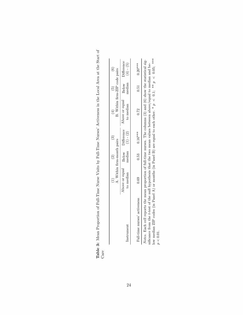
I illustrate how these two variations in the activeness instrument explain the proportion of
full-time nurse visits in Table 3. Panel A shows that in ZIP codes where full-time nurses
were more active (i.e. above or equal to median), patients had 16 percentage points higher
proportion of full-time nurse visits even within the same firm-month pairs. The median
values are created for each firm-month pair using the patient’s start-of-care month. The
difference is statistically significant at the one percent level by the t-test of the equality of the
means. Panel B shows that when patients happened to start care in months during which
13
full-time nurses were more active, they received 20 percentage points higher proportion of
full-time nurse visits within the same firm-ZIP code pairs. This difference is also statistically
significant at the one percent level.
1.5.2. Empirical Specifications
First, I model the first-stage relationships between the patient i’s proportion of full-time
nurse visits FTVi and the instrument variable Zi, Activei, at the patient episode level. For
each patient episode i who is served by firm fpiq, lives in ZIP code zpiq, and has her home
health care start in month mpiq and end in time period tpiq, her proportion of full-time
nurse visits FTVi is a function of the form:
FTVi “ α0 ` α1Zi ` γXi ` δfpiq ` ζzpiq ` ηmpiq ` θtpiq ` νi,fpiq,zpiq,mpiq,tpiq. (1.2)
The vector Xi includes observed patient characteristics including the number of nurse hand-
offs, total number of nurse visits, mean interval of nurse visits (i.e. mean number of days
between two consecutive nurse visits), a set of firm level service demand and labor demand
characteristics, a set of hospitalization risk controls, a set of demographic controls, and a
set of comorbidity controls. The set of firm level service demand and labor demand controls
includes mean of firm-day level variables capturing the caseload and labor supply conditions
in each firm across the patient’s home health days. The firm-day level variables include the
number of ongoing episodes, the number of active nurses, and the fraction of active piece-
rate nurses working in an firm-day cell. The set of hospitalization risk controls represents a
set of indicator variables associated with high risk of hospitalization, and includes history
of 2 or more falls in the past 12 months, 2 or more hospitalizations in the past 6 months, a
decline in mental, emotional, or behavioral status in the past 3 months, currently taking 5
or more medications, and others. The set of demographic controls includes six 5-year age
group dummies for ages ranging from 65-94 (age 95 or higher is an omitted group), gender,
race, insurance type, an indicator for having no informal care assistance available, and an
14
indicator for living alone.13 The set of comorbidity controls includes a Charlson comor-
bidity index, indicators for overall health status, indicators for high-risk factors including
alcohol dependency, drug dependency, smoking, obesity, and indicators for conditions prior
to hospital stay within past 14 days including disruptive or socially inappropriate behav-
ior, impaired decision making, indwelling or suprapublic catheter, intractable pain, serious
memory loss and/or urinary incontinence.14 νi,fpiq,zpiq,mpiq,tpiq is an idiosyncratic error.
Controlling for the number of handoffs and total number of nurse visits in the regression
equation is important. Experiencing a mix of permanent and temporary labor during patient
care inevitably involves switching of providers or “handoffs,” which may independently affect
the patient outcome. Fewer handoffs mechanically lead to either one or zero proportion of
full-time nurse visits: this is illustrated in Table 2 with much smaller ratio of handoffs
to nurse visits for Groups 1 and 4, who received zero and 100 percent of full-time nurse
visits, respectively. In Chapter 3 of this dissertation, I find nurse handoffs—defined as being
visited by a different nurse than the last one—to substantially increase the probability of
readmission.15 In addition, sicker patients may receive more nurse visits, which affects the
proportion of full-time nurse visits and the likelihood of readmission.
I also include a set of fixed effects for firm, patient ZIP code, start-of-care month, and
end-of-care time period, where the time period refers to the day of week (6 dummies), week
of year (52 dummies), and year (4 dummies). Therefore, this estimation compares patients
in two ways, as explained above. First, it compares patients who were served by the same
firm, started care in the same month and ended home health care at the same time but lived
in different ZIP codes having a different level of activeness or preoccupied nearest full-time
13Insurance types include Medicare Advantage (MA) plans with a visit-based reimbursement, MA planswith an episode-based reimbursement, and dual eligible with Medicaid enrollment (reference group is Medi-care FFS).
14Indicators for overall health status include indicators for very bad (patient has serious progressive con-ditions that could lead to death within a year), bad (patient is likely to remain in fragile health) andtemporarily bad (temporary facing high health risks).
15Although handoffs are found to be an important determinant of readmission in Chapter 3, I do not treatit as an endogenous variable to be instrumented for in this specification. The reason is that my instrumentfor the proportion of full-time nurses poorly capture the variation of handoffs. Since the causal effect ofhandoffs is not of main interest in this chapter, I just control for it as an explanatory variable.
15

nurses. Second, the regression compares patients who were served by the same firm, lived
in the same ZIP code, and ended home health care at the same time but had a different
level of activeness or preoccupied nearest full-time nurses at the start of care.
The main estimating model for the second-stage relationship between the proportion of
full-time nurse visits and patient readmission takes the form
Readmiti “ β0 ` β1FTVi ` γXi ` δfpiq ` ζzpiq ` ηmpiq ` θtpiq ` εi,fpiq,zpiq,mpiq,tpiq. (1.3)
where Readmiti is an indicator variable for hospital readmission of a patient episode i. I
compare the OLS estimation of equation 1.3 with its 2SLS estimation using the instruments
explained above. This comparison will show the importance of taking into account the non-
random assignment of full-time nurse visits in identifying the effect of labor mix on patient
readmission. I estimate a linear probability model.
1.5.3. Potential Limitations
There are potential concerns about the instruments. First, there could be unobserved ZIP
code-month level shocks that are correlated with the full-time nurses’ activeness and the
patient readmission. For example, do demographic changes such as a surge in the elderly
population in a given ZIP code-month pair affect both full-time nurses’ activeness and
patient readmission? A lack of availability of such high-frequency ZIP code level information
makes it hard to directly control for these relevant ZIP code-month level controls. However,
for example, if an elderly population grows in a ZIP code in a given month, the omitted
variable bias is expected to work against finding a negative effect of full-time nurse visits on
readmission. The reason is that full-time nurses would become more active due to increased
home health care demand while the readmission would be more likely among the elderly.
Second, firms may selectively admit patients into home health care based on the full-time
nurses’ activeness. To the extent that firms admit healthier patients into home health care
when full-time nurses were more active, I will likely overstate the negative effect of full-
16
time nurse visits on patient readmission. To allay this concern, I investigate the balancing
of observed characteristics by whether the patient had high or low activeness of full-time
nurses. High values are marked by whether the activeness is above or equal to median.
Table 4 reports the mean values of regression controls for the two groups of patients. The
first row in Panel A shows that when full-time nurses are more active, patients’ proportion
of full-time nurse visits is higher, as expected. When patients had high activeness of full-
time nurses, they had nearly double the proportion of full-time nurse visits in column (2)
by 40 percentage points, compared to patients who had low activeness in column (1). The
hospital readmission rate is also greater for patients with high activeness of full-time nurses.
Simultaneously, the hospitalization risk factors in Panel C and comorbidity characteristics
in Panel E show that patients with high activeness of full-time nurses were indeed sicker.
On average, these patients had higher Charlson comorbidity index and higher likelihood of
having their overall status to remain in fragile health. Thus, I can refute the concern that
firms may selective admit healthier patients when full-time nurses are more active. It was
rather the opposite: firms tended to admit sicker patients when full-time nurses were more
active, which works against finding a negative effect of full-time nurse visits on readmission.
1.6. Results
1.6.1. First-Stage Results on the Proportion of Full-Time Nurse Visits
Table 5 shows the first-stage results on the relationship between the proportion of full-
time nurse visits and my instrument—full nurses’ activeness in the patient’s ZIP code—in
equation (1.2). Standard errors in these models are clustered at both the firm and patient
ZIP code levels.
In column (1), I begin by estimating the equation with fixed effects for each firm and ZIP
code, respectively, and end-of-care time fixed effects for the week of year, year, and day of
week. I also control for the number of nurse handoffs, total number of nurse visits, mean
interval of nurse visits and office-week level overall demand and labor supply characteristics.
17

I incrementally control for more patient characteristics in columns (2)–(4).
There is a strong correlation between the patient’s proportion of full-time nurse visits and
my instrument, as shown by the statistically significant correlations at the one percent
level and large F-statistic values of around 300. In column (4) for the richest specification,
when full-time nurses were more active in the patient’s ZIP code during the start-of-care
month by one standard deviation (0.26), she received 16 percentage points or 26 percent
higher proportion of full-time nurse visits given the mean of 0.6.16 This would translate to
nearly one more full-time nurse visit during her care which involved six total nurse visits
on average.
1.6.2. Second-Stage Results on Patient Readmission
I begin with the OLS estimation of the effect of the proportion of full-time nurse visits
on patient readmission in equation (1.3). Panel A shows that the proportion of full-time
nurse visits is negatively correlated with an indicator for hospital readmission: patients
receiving a one-standard-deviation higher proportion of full-time nurse visits (0.41) were
0.4 percentage points or 2 percent less likely to be readmitted given the mean readmission
rate of 0.2. However, this effect is not statistically significant even at the 10 percent level
in all columns. This result reflects the upward bias I described in Section 1.4, which likely
occurs since sicker patients tended to have a higher proportion of full-time nurse visits.
Indeed, the coefficient decreases twofold from column (1) to (2), and threefold from column
(1) to (4). This pattern corroborates that sicker patients in terms of hospitalization risk
controls, demographic controls and comorbidity controls were systematically assigned a
higher proportion of full-time nurse visits while those patients were independently more
likely to be readmitted.
Panel B shows the 2SLS estimates using the first-stage results from Table 5. There is a
stronger negative correlation between the proportion of full-time nurse visits and hospital
16A 26-percent increase is obtained by multiplying the one standard deviation, 0.26, by the coefficientestimate 0.608 and dividing by the mean proportion of full-time nurse visits 0.6 (with the final numbermultipled by 100 for the percentage).
18

readmission by almost four times. The effects are statistically significant at the ten per-
cent level once hospitalization risk, demographic, and comorbidity controls are included in
columns (2)–(4). The rise of statistical significance reflects, shown in Section 1.5.3, that
sicker patients were more likely to be admitted when full-time nurses were active—which
works against estimating a negative effect of full-time nurse visits on readmission. This
pattern also contributes to reducing the precision of the estimates. On the other hand,
the estimated effects of full-time nurse visits on readmission can be viewed as conservative.
From the richest specification in column (4), I find that patients having a one-standard-
deviation (0.41) higher proportion of full-time nurse visits or about 2 more full-time nurse
visits were 1.4 percentage points or 7 percent less likely to be readmitted.
1.7. Conclusion
Alternative work arrangements are becoming increasingly popular modes of labor contracts
in many industries due to the appeal of the flexibility and potential labor cost reductions.
Health care, a labor-intensive service industry facing demand uncertainty, particularly has
experienced one of the largest increases in the use of alternative work arrangements over the
past two decades. These arrangements might be particularly necessary for supplementing
labor supply in the presence of state regulations of the minimum nurse staffing levels and
staffing shortages (Tong, 2011; Cook et al., 2012; Mark et al., 2013; Lin, 2014; Matsudaira,
2014). Therefore, it is crucial to understand whether providers hired in traditional and
alternative work arrangements lead to any difference in the quality of care and performance.
However, estimating this hypothesis is challenging due to confounding factors and non-
random matching of patients and providers in particular work arrangements, as described
above. Home health care and the dataset I use provide an ideal opportunity to overcome
these challenges and investigate the effect of full-time nurse visits on patient readmission.
Home health is also an important market to study as it is one of the fastest growing sectors
of health care, and is a sector in which a large proportion of the workforce is hired in
alternative work arrangements.
19

I find that patients receiving a higher proportion of full-time nurse visits were less likely to be
readmitted. This finding is obtained by exploiting an exogenous variation across ZIP codes
and care timings in the proportion of full-time nurse visits from full-time nurses’ activeness.
Moreover, this effect holds after controlling for patients’ underlying health characteristics,
office-level demand and labor supply characteristics, patients’ ZIP code fixed effects, firm
fixed effects, month fixed effects and fixed effects related to the timings of the start and end
of care.
My findings suggest that increasing the use of full-time nurses can improve the quality of
care. It will be a fruitful target for policymakers and providers to focus on understanding
the determinants of and reducing the gap in quality provided by nurses in different work
arrangements. Consequently, future work on the specific mechanisms underlying my find-
ing is critical. If experience were an important determinant of quality difference between
full-time nurses and others, it is crucial to investigate nurses’ learning curve, which also
has broader implication on the choice of work arrangements and the value of retention.
Furthermore, future work on the variation in the gap in quality of care among nurses in
different work arrangements across different firms is crucial. Organizational learning by
doing on the management and configuration of alternative work arrangements will provide
valuable insights.
20

Figure 1: Variation in the Proportion of Full-Time Nurse Visits across PatientEpisodes
0.0
0.2
0.4
0.6
0.8
1.0
0.0 0.2 0.4 0.6 0.8 1.0
Proportion of full−time nurse visits
Fra
ctio
n
Notes: The unit of observation is a patient episode. The vertical line denotes the median value, 0.75.
21

Table 1: Labor Supply and Pay Characteristics of Nurses by Work Arrange-ments
(1) (2) (3) (4) (5) (6)
Full-time
Part-timewith
benefits
Part-timewithoutbenefits On-call Contractor
Office/
Other
A. Labor supply characteristics per weekNumber of visits 21.84 15.93 14.53 8.93 6.46 10.76Number of days worked 4.95 4.51 4.35 3.45 2.27 3.40Total time spent on visits (hours) 16.16 12.15 11.49 6.94 5.57 8.24Mean visit length (hours) 0.77 0.79 0.80 0.84 0.87 0.85Length of employment (months) 21.18 24.41 28.29 16.29 5.18 8.33
B. Pay characteristicsPay scheme Salary Salary Salary Piece rate Piece rate SalaryTotal weekly pay ($) 1,239.27 819.25 711.91 445.06Per visit rate ($) 43.77 42.30 42.70 55.80
Notes. The first four variables in Panel A are obtained using weeks during which the nurses provided atleast one visit. The length of employment in Panel A is measured for nurses who terminated their employ-ment, where the termination is defined as either permanently exiting the workforce or providing no visitsfor more than 90 consecutive days. For the pay scheme in Panel B, salary is defined as a fixed amount ofpay for the specific expected number of visits per week, and piece rate as a fixed rate per visit. Salariednurses are eligible for benefits, except part-time nurses without benefits in column (3); piece-rate paidones are ineligible.
22
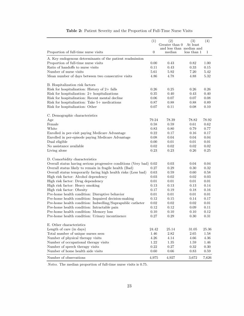
Table 2: Patient Severity and the Proportion of Full-Time Nurse Visits
(1) (2) (3) (4)
Proportion of full-time nurse visits 0
Greater than 0and less than
median
At leastmedian andless than 1 1
A. Key endogenous determinants of the patient readmissionProportion of full-time nurse visits 0.00 0.43 0.82 1.00Ratio of handoffs to nurse visits 0.11 0.43 0.33 0.15Number of nurse visits 5.61 5.92 7.20 5.42Mean number of days between two consecutive visits 4.86 4.78 4.88 5.32
B. Hospitalization risk factorsRisk for hospitalization: History of 2+ falls 0.26 0.25 0.26 0.26Risk for hospitalization: 2+ hospitalizations 0.35 0.40 0.43 0.40Risk for hospitalization: Recent mental decline 0.06 0.07 0.07 0.08Risk for hospitalization: Take 5+ medications 0.87 0.88 0.88 0.89Risk for hospitalization: Other 0.07 0.11 0.08 0.10
C. Demographic characteristicsAge 79.24 78.39 78.82 78.92Female 0.58 0.59 0.61 0.62White 0.83 0.80 0.79 0.77Enrolled in per-visit paying Medicare Advantage 0.22 0.17 0.16 0.17Enrolled in per-episode paying Medicare Advantage 0.08 0.04 0.04 0.04Dual eligible 0.00 0.01 0.01 0.01No assistance available 0.02 0.02 0.02 0.02Living alone 0.23 0.23 0.26 0.25
D. Comorbidity characteristicsOverall status having serious progressive conditions (Very bad) 0.02 0.03 0.04 0.04Overall status likely to remain in fragile health (Bad) 0.27 0.29 0.30 0.32Overall status temporarily facing high health risks (Less bad) 0.63 0.59 0.60 0.58High risk factor: Alcohol dependency 0.03 0.02 0.02 0.03High risk factor: Drug dependency 0.01 0.01 0.01 0.01High risk factor: Heavy smoking 0.13 0.13 0.13 0.14High risk factor: Obesity 0.17 0.19 0.18 0.16Pre-home health condition: Disruptive behavior 0.01 0.01 0.01 0.01Pre-home health condition: Impaired decision-making 0.12 0.15 0.14 0.17Pre-home health condition: Indwelling/Suprapublic catheter 0.02 0.02 0.02 0.01Pre-home health condition: Intractable pain 0.12 0.12 0.09 0.11Pre-home health condition: Memory loss 0.10 0.10 0.10 0.12Pre-home health condition: Urinary incontinence 0.27 0.29 0.30 0.31
E. Other characteristicsLength of care (in days) 24.42 25.14 31.05 25.36Total number of unique nurses seen 1.46 2.82 2.65 1.58Number of physical therapy visits 4.26 4.14 4.66 4.36Number of occupational therapy visits 1.22 1.35 1.59 1.46Number of speech therapy visits 0.22 0.27 0.32 0.30Number of home health aide visits 0.60 0.66 0.83 0.59
Number of observations 4,975 4,927 3,672 7,626
Notes. The median proportion of full-time nurse visits is 0.75.
23
Table
3:
Mea
nP
rop
orti
onof
Fu
ll-T
ime
Nurs
eV
isit
sby
Fu
ll-T
ime
Nu
rses
’A
ctiv
enes
sin
the
Loca
lA
rea
at
the
Sta
rtof
Car
e
(1)
(2)
(3)
(4)
(5)
(6)
A.
Wit
hin
firm
-month
pair
sB
.W
ithin
firm
-ZIP
code
pair
s
Inst
rum
ent
Ab
ove
or
equal
tom
edia
nB
elow
med
ian
Diff
eren
ce(1
)-
(2)
Ab
ove
or
equal
tom
edia
nB
elow
med
ian
Diff
eren
ce(4
)-
(5)
Full-t
ime
nurs
es’
act
iven
ess
0.6
90.5
30.1
6***
0.7
20.5
10.2
0***
Notes.
Each
cell
rep
ort
sth
em
ean
pro
port
ion
of
full-t
ime
nurs
es.
The
colu
mns
(3)
and
(6)
show
the
stati
stic
al
sig-
nifi
cance
from
thet-
test
of
the
null
hyp
oth
esis
that
the
two
mea
nva
lues
bet
wee
nab
ove/
equal
tom
edia
nand
be-
low
med
ian
ZIP
codes
(in
Panel
A)
or
month
s(i
nP
anel
B)
are
equal
toea
choth
er.
*p
ă0.1
;**p
ă0.0
5;
***
pă
0.0
1.
24
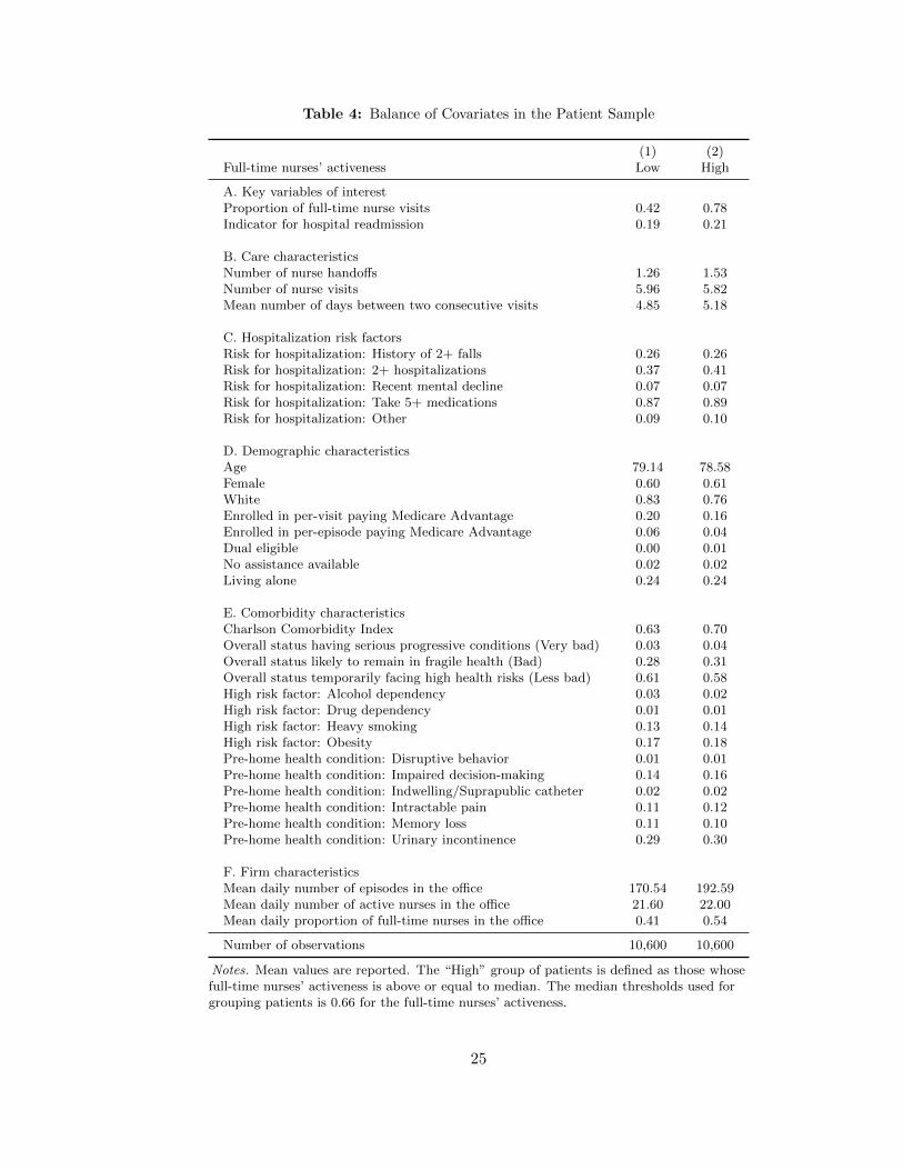
Table 4: Balance of Covariates in the Patient Sample
(1) (2)Full-time nurses’ activeness Low High
A. Key variables of interestProportion of full-time nurse visits 0.42 0.78Indicator for hospital readmission 0.19 0.21
B. Care characteristicsNumber of nurse handoffs 1.26 1.53Number of nurse visits 5.96 5.82Mean number of days between two consecutive visits 4.85 5.18
C. Hospitalization risk factorsRisk for hospitalization: History of 2+ falls 0.26 0.26Risk for hospitalization: 2+ hospitalizations 0.37 0.41Risk for hospitalization: Recent mental decline 0.07 0.07Risk for hospitalization: Take 5+ medications 0.87 0.89Risk for hospitalization: Other 0.09 0.10
D. Demographic characteristicsAge 79.14 78.58Female 0.60 0.61White 0.83 0.76Enrolled in per-visit paying Medicare Advantage 0.20 0.16Enrolled in per-episode paying Medicare Advantage 0.06 0.04Dual eligible 0.00 0.01No assistance available 0.02 0.02Living alone 0.24 0.24
E. Comorbidity characteristicsCharlson Comorbidity Index 0.63 0.70Overall status having serious progressive conditions (Very bad) 0.03 0.04Overall status likely to remain in fragile health (Bad) 0.28 0.31Overall status temporarily facing high health risks (Less bad) 0.61 0.58High risk factor: Alcohol dependency 0.03 0.02High risk factor: Drug dependency 0.01 0.01High risk factor: Heavy smoking 0.13 0.14High risk factor: Obesity 0.17 0.18Pre-home health condition: Disruptive behavior 0.01 0.01Pre-home health condition: Impaired decision-making 0.14 0.16Pre-home health condition: Indwelling/Suprapublic catheter 0.02 0.02Pre-home health condition: Intractable pain 0.11 0.12Pre-home health condition: Memory loss 0.11 0.10Pre-home health condition: Urinary incontinence 0.29 0.30
F. Firm characteristicsMean daily number of episodes in the office 170.54 192.59Mean daily number of active nurses in the office 21.60 22.00Mean daily proportion of full-time nurses in the office 0.41 0.54
Number of observations 10,600 10,600
Notes. Mean values are reported. The “High” group of patients is defined as those whosefull-time nurses’ activeness is above or equal to median. The median thresholds used forgrouping patients is 0.66 for the full-time nurses’ activeness.
25

Table 5: IV First-Stage Results: Effect of Full-time Nurses’ Activeness on the Proportion ofFull-Time Nurse Visits
Dep. var.: Proportion of full-time nurse visits(1) (2) (3) (4)
Full-time nurses’ activity share 0.602*** 0.602*** 0.602*** 0.600***(0.034) (0.035) (0.035) (0.035)
R-squared 0.32 0.32 0.33 0.33F-statistic 307.20 301.83 299.66 301.47
Hospitalization risk controls . Yes Yes YesDemographic controls . . Yes YesComorbidity controls . . . YesObservations 21,200 21,200 21,200 21,200
Source. Authors’ proprietary data. Notes. The unit of observation is a patient episode.In all columns, I control for the number of nurse handoffs, total number of nurse visits,mean interval of nurse visits, mean of firm-day level demand and labor supply character-istics during the patient’s episode; and firm fixed effects, patient’s ZIP code fixed effects,fixed effects for day of week, week of year, and year of the last day of care, respectively.Firm-ZIP code level clustered standard errors in parentheses. * p ă 0.1; ** p ă 0.05;*** p ă 0.01.
26

Table 6: Main Results: Effect of Proportion of Full-Time Nurse Visits onPatient Readmission
Dep var: Indicator for hospital readmission(1) (2) (3) (4)
A. OLS
Proportion of full-time nurse visits -0.003 -0.007 -0.007 -0.009(0.013) (0.010) (0.010) (0.009)
R-squared 0.13 0.15 0.15 0.18
B. 2SLS
Proportion of full-time nurse visits -0.032 -0.036* -0.035* -0.035*(0.021) (0.020) (0.020) (0.020)
R-squared 0.02 0.02 0.02 0.02
Hospitalization risk controls . Yes Yes YesDemographic controls . . Yes YesComorbidity controls . . . YesObservations 21,200 21,200 21,200 21,200
Source. Authors’ proprietary data. Notes. The unit of observation is a patientepisode. I use a a two-step efficient generalized method of moments (GMM) estimator.In all columns, I control for the number of nurse handoffs, total number of nurse visits,mean interval of nurse visits, mean of firm-day level demand and labor supply charac-teristics during the patient’s episode; and firm fixed effects, patient’s ZIP code fixedeffects, fixed effects for day of week, week of year, and year of the last day of care, re-spectively. Firm-ZIP code level clustered standard errors in parentheses. * p ă 0.1; **p ă 0.05; *** p ă 0.01.
27

CHAPTER 2 : The Effect of Reputation on Firms’ Labor Mix Strategy under De-
mand Uncertainty
2.1. Introduction
One of the fundamental challenges for labor-intensive service firms facing demand uncer-
tainty is how to configure their workforce to improve service quality and performance. In
particular, such firms must decide on a mix of temporary and permanent workers to deal
with fluctuations in demand. Existing economic literature has shown that firms rely more on
temporary workers when facing greater demand fluctuations due to either the opportunity
cost of keeping an idle workforce (Dixit and Pindyck, 1994; Foote and Folta, 2002; Lotti
and Viviano, 2012) or the cost associated with high turnover rate (Rebitzer and Taylor,
1991; Levin, 2002). However, this does not take into account that permanent and tempo-
rary workers may not be perfectly interchangeable in production. In particular, there is
evidence that permanent workers outperform temporary workers in terms of the quality of
service provided, as shown in Chapter 1 of this dissertation (Bae et al., 2010; Pham et al.,
2011; Lotti and Viviano, 2012; Lu and Lu, 2016). Thus, how firms configure their workforce
depends crucially on the following trade-off: temporary workers provide greater flexibility
in responding to fluctuation in demand but may impede the establishment of firm reputa-
tion through lower quality of service. Despite the salience of this trade-off—particularly to
younger firms, which face both greater demand fluctuations and a greater need to demon-
strate high quality to their clientele—its incorporation is largely absent from the existing
literature. This may be due to a paucity of high-frequency longitudinal data containing
firms’ labor configurations and patient demand allocation. In this chapter, using novel data
from the home health industry, I aim to fill this gap and paint a more complete picture of
service firms’ temporary labor strategy.
I present and test a simple model of firms’ labor mix choices, highlighting the role of reputa-
tion in determining how firms optimally balance the trade-off between responding to demand
28
shocks and improving quality. Vast literature has shown the crucial role of reputation in
determining quality (Klein and Leffler, 1981; Carmichael, 1984; McMillan and Woodruff,
1999; Banerjee and Duflo, 2000; Baker et al., 2002; Macchiavello and Morjaria, 2015) and
demand (Navathe and David, 2009; Johnson, 2011) in the presence of non-enforceable con-
tracts. In service industries, demand is often non-contractible either due to the nature of
service provision, organizational structure or a regulatory ban. Thus, the perception of a
firm’s service quality, which forms a basis of the firm’s reputation, becomes an important de-
terminant of demand faced by the firm. Particularly in health care, provider firms compete
on quality since prices are often administered and consumers show little price sensitivity
due to generous health insurance. The competitive reallocation forces have been shown to
encourage providers to improve quality (Johnson, 2011; Chandra et al., 2016). Therefore,
reputation concerns are likely to prevail in health care and shape firms’ labor mix decisions
in the presence of trade-offs in using temporary workers.
To build intuition for the role of reputation in determining firms’ labor mix choices, consider
the start-ups Munchery and Instacart, which provide on-demand grocery delivery service.
These start-ups initially used independently contracted drivers to perform all the tasks.
However, due to high turnover and quality deterioration, the firms completely eliminated or
diminished the role of temporary workers particularly in tasks that are likely to determine
the quality of service.1 These cases suggest that the importance of reputation building
among starting firms makes them prioritize providing higher quality over purely optimizing
cost and rely more on permanent workers.
Making this intuition more rigorous, my model posits that a firm’s labor mix influences the
market’s perception of the firm’s quality, and the firm’s demand is in turn stochastically
linked to its reputation for quality. Underlying this mechanism is a process of dynamic
reputation formation in which the market observes the firm’s quality signals and updates
the firm’s reputation. This model is built on Navathe and David (2009)’s model of physi-
1“A middle ground between contract worker and employee” by Noam Scheiber, New York Times, De-cember 10, 2015.
29
cians’ technology adoption behavior under reputation concerns but I extend the model to
a stochastic optimal control problem to incorporate demand uncertainty.
I explicitly model the trade-off involved in the labor mix choice. On the one hand, the
proportion of demand served by permanent workers increases quality signals, and thus
increases reputation. This key assumption is supported by my finding in Chapter 1 of
this dissertation. I find that patients receiving a higher proportion of full-time nurse visits
during care were less likely to be readmitted to a hospital. This evidence validates my model
assumption and validates my claim that firms are faced with a trade-off in using temporary
workers between flexibility and quality.
On the other hand, permanent workers reduce the firm’s expected short-term profitability
since the firm hires them before observing the demand realization. Therefore, the firm
optimally balances across time the long-term reputation gain from increasing the share of
permanent workers with the reduction in short-term profitability. The central predictions
of the model are that firms with lower reputation increase the share of permanent workers
in response to demand volatility to achieve long-term gain in reputation. In contrast, firms
with higher reputation decrease the share of permanent workers to reduce short-term profit
loss.
I test the predictions of the model using data from a large US home health provider operating
106 autonomous offices in 18 states during 2012-2015. Each office with its own director
having full authority on the labor configuration and management is treated as a separate
firm. The data contain the entire home health visit records in each firm showing all the
interactions between a patient and individual providers who served her, as well as human
resources characteristics such as providers’ employment arrangements and weekly pays.
Moreover, for each patient, the data contain referral sources, which allow me to track the
establishment of strong referral networks in each firm and use this as a proxy for the firm’s
reputation. I can measure reputation in various ways: the size of referral network, referral
dispersion, referral consistency, and referral share from each source. Combining these data,
30

I construct weekly longitudinal data for each firm containing labor configuration, demand
environments, as well as measures of reputation.
In the cross-sectional analysis with firm fixed effects, I examine the relationship between
firms’ percentage of full-time nurses and demand volatility, and whether this relationship
varies with various measures of reputation. I find evidence consistent with both predictions
of my model. I find that firms with a lower reputation stock increased the percentage of
full-time nurses with demand volatility. Firms in the bottom third of the within-firm age-
specific distribution in terms of referral network size and referral consistency hired 0.2-0.3
more full-time nurse in the mean nursing workforce size of 21 nurses when demand volatility
increased by one standard deviation. In particular, young firms aged 0–12 months hired
0.5 to 1 more full-time nurses and hired 0.5 fewer contractor nurses given the mean total
workforce size of 13 nurses when demand volatility increased by one standard deviation.
Considering firms’ age as a proxy of reputation, this stronger correlation among the young
firms provides further support to my model. Moreover, this result was not confounded by
the size effect: it was only the large young firms that hired more full-time nurses when they
had a small referral network and low referral consistency. In contrast, I find the positive
association between the percentage of full-time nurses and demand volatility disappears
when firms’ reputation increased. These results suggest that low-reputation firms forgo
short-term profitability to achieve long-term reputation through quality improvement.
This chapter contributes novel empirical evidence that firms’ labor mix strategies crucially
depend on their reputation and provides a theoretical model to explain this. Although
traditional theory suggests that firms should decrease the share of permanent labor in the
face of increased demand volatility, my data indicate the opposite and counterintuitive story.
Less established firms such as starting firms rather increase the share of permanent workers
in response to demand volatility. This phenomenon cannot be explained if only demand
shocks are considered as a determinant of labor mix. I propose that this may be explained
by taking into consideration a firm’s concern for building reputation.
31

This chapter is related to and builds upon several topics in the literature. Most closely
related is work studying the relationship between demand uncertainty and labor input
choices (Rebitzer and Taylor, 1991; Abraham and Taylor, 1996; Levin, 2002; Lotti and
Viviano, 2012) and more broadly work on input choice under uncertainty (Oi, 1961; Nadiri
and Rosen, 1973; Sandmo, 1971; Batra and Ullah, 1974; Hartman, 1976; Friedman and
Pauly, 1981; Guiso and Parigi, 1999; Baker et al., 2004). The chapter is also related to
literature on the role of reputation in determining firms’ quality or commitment to non-
enforceable contracts (Klein and Leffler, 1981; McMillan and Woodruff, 1999; Banerjee and
Duflo, 2000; Navathe and David, 2009; Johnson, 2011; Macchiavello and Morjaria, 2015).
The remainder of this chapter is organized as follows. In Section 2.2, I provide background
on home health care and the employment arrangements used by home health firms in the
data. In Section 2.3, I present a model of firms’ labor mix choices. In Section 2.4, I
describe the data and sample restriction rules. In Section 2.5, I describe the evolution of
firm’s demand volatility, labor mix, and reputation by firm age. In Section 2.6, I conduct
empirical analysis of the effect of reputation on firms’ labor mix and report results. In
Section 2.7, I discuss possible alternative explanations for my empirical results and conduct
robustness checks. In Section 2.8, I conclude the chapter.
2.2. Background on Home Health Care
Home health care, which is provided to homebound patients who need skilled nursing or
therapy services, is an important and rapidly growing segment of the post-acute care delivery
system. I provide more details on the home health care industry and home health care
professionals in Appendices A.1 and A.2, respectively, at the end of the dissertation.
Home health is an ideal setting to investigate the impact of reputation on firms’ labor
mix choices. It is labor intensive, less technology-dependent, and decentralized (David and
Polsky, 2014), as patients receive services in their homes, making it easier to attribute
patient outcomes to workforce configuration. Moreover, quality is a critical dimension
32
on which firms compete since public insurance, i.e. Medicare, is a primary payer with
prospective payment and thus prices are administered (Gaynor et al., 2014). Furthermore,
referrals from other health care facilities are a primary source of new demand for home
health care firms. However, the federal Anti-Kickback Statute bans formally contracting
with referral sources for the number of referrals, thus elevating the importance of reputation
as a driver of firms’ demand volume. The statute also has the effect of making demand
inherently uncertain and consequently increasing the importance of temporary labor as a
source of labor supply.
In this chapter, I focus on the skilled nursing workforce—combination of registered nurses
(RNs) and licensed practice nurses (LPNs)—since nurses provide the most medically rel-
evant service that could potentially determine hospital readmissions and accounts for a
majority of the home health visits. Thus, home health firms have the largest demand for
skilled nurses and maintain the largest capacity of them each week.
2.3. Theory
Consider a risk-neutral home health firm and many risk-neutral referral sources (e.g., hos-
pitals) which can refer patients to the firm and determine the quantity of home health
demand Qt faced by the firm in periods t “ 0, 1, . . . . A firm hires workers mainly in two
work arrangements: salary (for permanent positions) and piece-rate pay (for temporary
positions). The difference lies in the fact that salaried workers are hired before observing
demand while piece-rate paid workers can be hired after observing demand.
The sequence of events is as follows. At the beginning of a period t, the firm’s reputation
for quality among referral sources is Rt.2 The demand the firm faces is influenced by its
reputation, but remains stochastic overall. The firm must choose how many salaried workers
to hire in advance of observing the actual demand in period t. The market then views the
fraction of demand served by salaried workers as a quality signal and updates its judgment
2I assume the reputation in the initial period 0 to be some fixed value below the market average.
33

of the firm’s reputation for the next period accordingly.
In a little more detail, let st and pt denote labor demand for salaried and piece-rate paid
workers, respectively. Assume that the units of labor demand are equal to the units of home
health demand for simplicity. The firm hires salaried workers st before observing demand
Qt. The firm hires piece-rate labor pt if demand exceeds salaried labor, i.e. Qt ą st.
Therefore,
Qt ě minpst, Qtq ` pt. (2.1)
The firm’s proportion of salaried labor st{Qt impacts the firm’s reputation in the next
period t` 1.
Denote the price per unit of demand by α. The price is constant since the primary payer of
home health services is Medicare FFS, which has a prospective payment system. Assume
that this marginal revenue α exceeds the marginal cost of serving demand, i.e. marginal cost
of labor for either type of workers. Then it is always profitable to serve all the demand that
arrives at the firm. Thus, the firm does not turn away any patients, and the constraint (2.1)
always holds with equality.3 Rearranging terms, this means the temporary labor demand
pt is given by
pt “ Qt ´minpst, Qtq (2.2)
“
$
’
’
&
’
’
%
0 if st ě Qt
Qt ´ st otherwise
(2.3)
To model how the firm’s reputation for quality is formed over time, suppose that its repu-
tation stock dynamically evolves as a combination of the history of reputation stocks and
new quality signals. Thus, I can write the next period’s reputation stock Rt`1 as a function
3I conjecture that relaxing this assumption of no turning away of patients would reinforce the model’spredictions because low-reputation firms would also want to reduce turnaway probability in addition toincreasing the share of salaried labor.
34
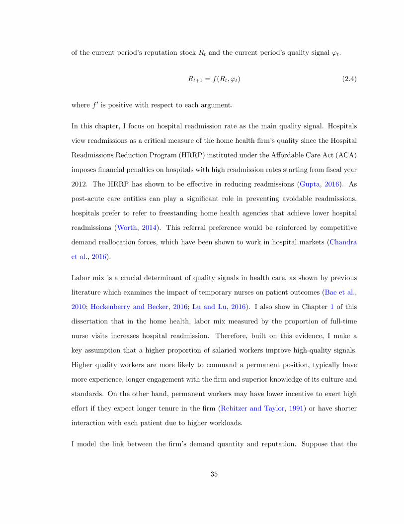
of the current period’s reputation stock Rt and the current period’s quality signal ϕt.
Rt`1 “ fpRt, ϕtq (2.4)
where f 1 is positive with respect to each argument.
In this chapter, I focus on hospital readmission rate as the main quality signal. Hospitals
view readmissions as a critical measure of the home health firm’s quality since the Hospital
Readmissions Reduction Program (HRRP) instituted under the Affordable Care Act (ACA)
imposes financial penalties on hospitals with high readmission rates starting from fiscal year
2012. The HRRP has shown to be effective in reducing readmissions (Gupta, 2016). As
post-acute care entities can play a significant role in preventing avoidable readmissions,
hospitals prefer to refer to freestanding home health agencies that achieve lower hospital
readmissions (Worth, 2014). This referral preference would be reinforced by competitive
demand reallocation forces, which have been shown to work in hospital markets (Chandra
et al., 2016).
Labor mix is a crucial determinant of quality signals in health care, as shown by previous
literature which examines the impact of temporary nurses on patient outcomes (Bae et al.,
2010; Hockenberry and Becker, 2016; Lu and Lu, 2016). I also show in Chapter 1 of this
dissertation that in the home health, labor mix measured by the proportion of full-time
nurse visits increases hospital readmission. Therefore, built on this evidence, I make a
key assumption that a higher proportion of salaried workers improve high-quality signals.
Higher quality workers are more likely to command a permanent position, typically have
more experience, longer engagement with the firm and superior knowledge of its culture and
standards. On the other hand, permanent workers may have lower incentive to exert high
effort if they expect longer tenure in the firm (Rebitzer and Taylor, 1991) or have shorter
interaction with each patient due to higher workloads.
I model the link between the firm’s demand quantity and reputation. Suppose that the
35

quantity of demand Qt is stochastically determined by reputation stock Rt:
Qt “ gpRtq (2.5)
where g1p¨q ą 0, implying that firms with greater reputation for quality receive higher
demand. This is a reasonable assumption since, with administered prices, firms compete on
non-price dimensions. It is standard to assume that the firm’s market share increases with
quality (Gaynor et al., 2014).
The firm’s objective is to maximize expected present discounted value of the profit subject
to the constraint (2.2):
VtpRtq “ maxtstu8t“0, tptu
8t“0
Eÿ
t
βtpαQtpRtq ´ cspstq ´ cppptqq (2.6)
subject to pt “ QtpRtq ´minpst, QtpRtqq. (2.7)
After plugging in the constraint (2.2) and rearranging terms, I obtain the following Bellman
equation:
VtpRtq “ maxst
Eπpst, Rtq ` βEV pRt`1q (2.8)
where
πpst, Rtq ” αQtpRtq ´ cspstq ´ cppQtpRtq ´minpst, QtpRtqqq.
In a general form, the expected profit for period t is given by
Eπpst, Rtq “ αQtpRtq ´ cspstq `
ż
QtpRtqąst
cppQtpRtq ´ stqdµpQtq (2.9)
where dµpQtq is a probability measure of Qt. To derive an analytic solution, assume that
36
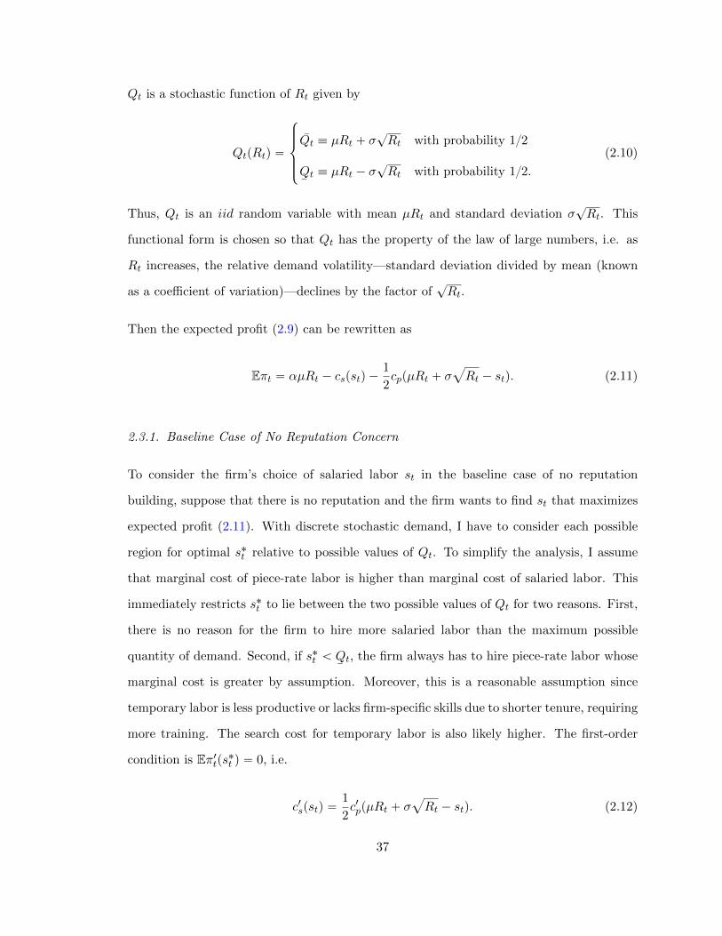
Qt is a stochastic function of Rt given by
QtpRtq “
$
’
’
&
’
’
%
Qt ” µRt ` σ?Rt with probability 1{2
¯Qt ” µRt ´ σ
?Rt with probability 1{2.
(2.10)
Thus, Qt is an iid random variable with mean µRt and standard deviation σ?Rt. This
functional form is chosen so that Qt has the property of the law of large numbers, i.e. as
Rt increases, the relative demand volatility—standard deviation divided by mean (known
as a coefficient of variation)—declines by the factor of?Rt.
Then the expected profit (2.9) can be rewritten as
Eπt “ αµRt ´ cspstq ´1
2cppµRt ` σ
a
Rt ´ stq. (2.11)
2.3.1. Baseline Case of No Reputation Concern
To consider the firm’s choice of salaried labor st in the baseline case of no reputation
building, suppose that there is no reputation and the firm wants to find st that maximizes
expected profit (2.11). With discrete stochastic demand, I have to consider each possible
region for optimal s˚t relative to possible values of Qt. To simplify the analysis, I assume
that marginal cost of piece-rate labor is higher than marginal cost of salaried labor. This
immediately restricts s˚t to lie between the two possible values of Qt for two reasons. First,
there is no reason for the firm to hire more salaried labor than the maximum possible
quantity of demand. Second, if s˚t ă¯Qt, the firm always has to hire piece-rate labor whose
marginal cost is greater by assumption. Moreover, this is a reasonable assumption since
temporary labor is less productive or lacks firm-specific skills due to shorter tenure, requiring
more training. The search cost for temporary labor is also likely higher. The first-order
condition is Eπ1tps˚t q “ 0, i.e.
c1spstq “1
2c1ppµRt ` σ
a
Rt ´ stq. (2.12)
37
The condition (2.12) shows that the optimal st equates the marginal cost of salaried labor,
which is non-stochastic and thus known precisely, with the expected marginal cost of piece-
rate paid labor. If one hires more salaried labor, the expected marginal savings from not
having to hire more expensive piece-rate labor increases. However, at a sufficiently high st,
the marginal cost of maintaining a salaried labor capacity becomes high enough to exceed
the expected marginal cost of piece-rate labor.
How does demand volatility σ affect firms’ relative use of piece-rate labor? Without repu-
tation concern, the firm would only want to minimize the sum of expected labor costs for
salaried and piece-rate labor. Since the firm hires piece-rate labor only when the demand
turns out high, one can expect that an increase in the volatility σ may increase both salaried
as well as piece-rate labor. This is expected given that they serve all the demand. Therefore,
one should examine how the relative demand for piece-rate labor changes. Indeed I find
that the firm increases the relative use of piece-rate labor as demand volatility increases
unless the rate of increase in the marginal cost for that labor is too high relatively. This
result is shown in Proposition 1. The proof is found in Appendix 2.9.
Proposition 1. Suppose that there is no reputation consequence from firms’ labor mix
choice. Then when demand volatility increases, the firm’s share of piece-rate labor increases
under the assumption that piece-rate labor does not become “too expensive.”
2.3.2. Case of Reputation Concern
Now to understand the firms’ optimal labor mix under reputation concerns, I first model
the firm’s reputation formation. I assume that quality signals ϕt are determined by the
proportion of cases served by salaried nurses as follows:
ϕt ” ϕ
ˆ
stQt
˙
“stAQt
,
38

where A is the market average of quality signals, which is the mean proportions of salaried
nurses in the market and thus lies between 0 and 1, inclusive. Furthermore, I assume the
formation of reputation in (2.4) follows the law of motion given by a Cobb-Douglas function
Rt`1 “ R1´γt
ˆ
stAQt
˙γ
. (2.13)
A reputation value of 1 corresponds to the market average A in terms of quality signals.
I assume the firm’s initial reputation is below average, that is R0 ă 1. Furthermore, note
that Rt is bounded above by 1A for all time. For Rt`1 is a weighted geometric average of Rt
and s{pAQq ď 1{A. So if Rt ď1A , then also Rt`1 ď
1A . Since we assumed R0 ă 1, it follows
by induction that Rt ď1A for all t. This upper bound on reputation stock and consequently
also quantity of demand guarantees compactness of the state space and justifies the use of
stochastic Bellman theory.
(2.13) assumes that reputation in the next period is updated using a geometric mean of the
current period’s reputation and quality signals to allow for different weights placed on the
history of reputation and quality signals. The smaller the weight γ on quality signals, the
more “sticky” the firm’s reputation is: the overall history of reputation is weighted more
than just the quality signal from the last period.
Let β P p0, 1q be a discount factor. By solving the Bellman equation in (2.8), I obtain the
first-order condition given by
E„
BπtBst
` βBRt`1
BstV 1pRt`1q
“ 0, (2.14)
and the envelope condition given by
V 1pRtq “ E„
BπtBRt
` βBRt`1
BRtV 1pRt`1q
. (2.15)
Combining the first-order condition and the envelope condition and advancing one period
39

forward, I obtain the Euler equation:
EBπtBst
“ βEˆ
BRt`1
Bst
˙„
Eˆ
Bπt`1
Bst`1
˙
EpBRt`2{BRt`1q
EpBRt`2{Bst`1q´ E
Bπt`1
BRt`1
(2.16)
The left-hand side of (2.16) represents the expected marginal profit from hiring one more
unit of salaried labor in period t:
EBπtBst
“ ´c1spstq `1
2c1ppµRt ` σ
a
Rt ´ stq ă 0. (2.17)
I assert that the sign of this expected marginal profit is negative for each t. It is not zero
when there is a reputation concern (i.e. right-hand side of (2.16) is nonzero). Moreover,
if it is positive, the firm always prefers to increase salaried labor because it increases both
the short-term profit and reputation, therefore facing no trade-off. Therefore, when there
is a reputation concern, increasing salaried labor reduces the firms’ short-term profit. Note
that this result can be compared with the case of having no reputation building where
Eπ1tps˚t q “ 0 is optimal.
On the right-hand side of (2.16), the factor
Eˆ
BRt`1
Bst
˙
“1
2
γ
A
ˆ
ARtst
˙1´γ
pQtpRtq´γ `
¯QtpRtq
´γq ą 0 (2.18)
is the reputation gain in the next period from increasing one unit of salaried labor in period
t. This scale is multiplied to the present discounted value of both future marginal profits
from increasing salaried labor (in the first term) and from increasing reputation (in the
second term) in the next period t ` 1 in the brackets. The first term in the brackets is a
product of two quantities: expected marginal profit per unit of increase in salaried labor in
the next period t` 1, and the marginal reputation gain two periods in the future t` 2 from
increasing t`1’s reputation relative to the gain from new quality signals in t`1. The ratio
measures a return on increasing salaried labor in t—how much the elevated base reputation
40
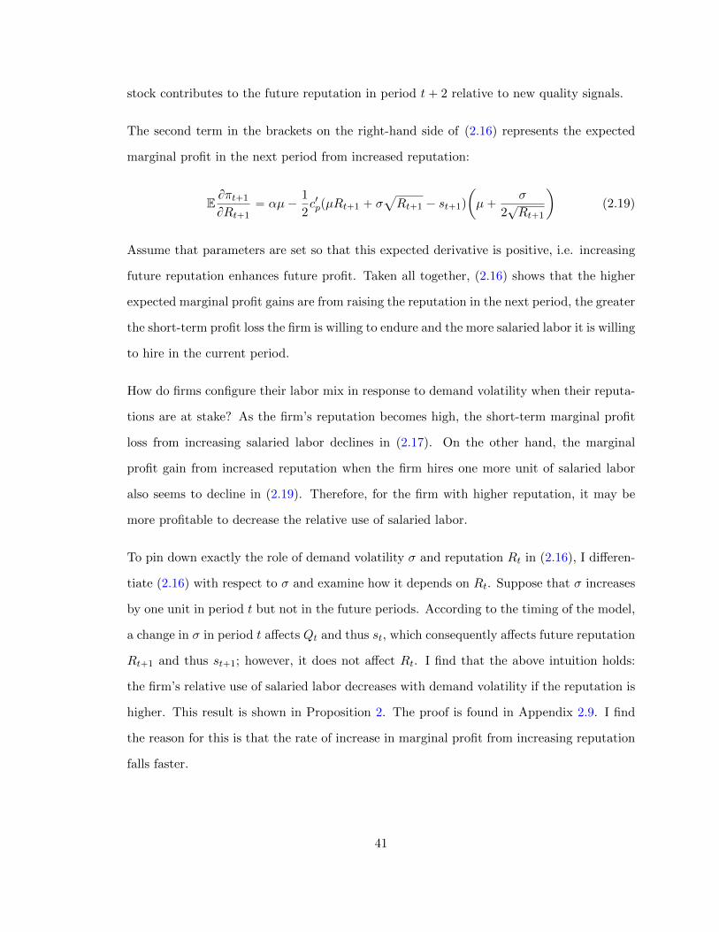
stock contributes to the future reputation in period t` 2 relative to new quality signals.
The second term in the brackets on the right-hand side of (2.16) represents the expected
marginal profit in the next period from increased reputation:
EBπt`1
BRt`1“ αµ´
1
2c1ppµRt`1 ` σ
a
Rt`1 ´ st`1q
ˆ
µ`σ
2?Rt`1
˙
(2.19)
Assume that parameters are set so that this expected derivative is positive, i.e. increasing
future reputation enhances future profit. Taken all together, (2.16) shows that the higher
expected marginal profit gains are from raising the reputation in the next period, the greater
the short-term profit loss the firm is willing to endure and the more salaried labor it is willing
to hire in the current period.
How do firms configure their labor mix in response to demand volatility when their reputa-
tions are at stake? As the firm’s reputation becomes high, the short-term marginal profit
loss from increasing salaried labor declines in (2.17). On the other hand, the marginal
profit gain from increased reputation when the firm hires one more unit of salaried labor
also seems to decline in (2.19). Therefore, for the firm with higher reputation, it may be
more profitable to decrease the relative use of salaried labor.
To pin down exactly the role of demand volatility σ and reputation Rt in (2.16), I differen-
tiate (2.16) with respect to σ and examine how it depends on Rt. Suppose that σ increases
by one unit in period t but not in the future periods. According to the timing of the model,
a change in σ in period t affects Qt and thus st, which consequently affects future reputation
Rt`1 and thus st`1; however, it does not affect Rt. I find that the above intuition holds:
the firm’s relative use of salaried labor decreases with demand volatility if the reputation is
higher. This result is shown in Proposition 2. The proof is found in Appendix 2.9. I find
the reason for this is that the rate of increase in marginal profit from increasing reputation
falls faster.
41
Proposition 2. Firms decrease the share of salaried labor when demand volatility increases
if their reputation is higher. Conversely, the firm’s share of salaried labor increases with
demand volatility if the reputation is lower.
2.3.3. Summary
The model makes the following testable predictions:
(i) When firms’ reputation is lower, higher demand volatility decreases firms’ share of
piece-rate paid labor and increases firms’ share of salaried labor.
(ii) When firms’ reputation is higher, higher demand volatility increases firms’ share of
piece-rate paid labor and decreases firms’ share of salaried labor.
2.4. Data
My primary data source is rich proprietary data from a large US for-profit freestanding
home health provider firm operating 106 autonomous offices in 18 states, which contain
firms’ labor configuration and patients’ outcomes in each office at an unusual level of detail.4
Since each office autonomously decides scheduling and staffing and is run as a profit center,
it is regarded as a separate firm in the empirical analysis.5 The data cover years 2012–2015.
My data contain the entire home health visit records in each office showing all the interac-
tions between a patient and individual providers who served her. I match these visit-level
data with the human resources data containing the history of employment arrangements
for each provider. Thus, I can construct weekly panel data for firms showing demand and
labor supply characteristics at the firm-week level. On the demand side, I can observe the
4These 18 states are Arizona, Colorado, Connecticut, Delaware, Florida, Hawaii, Massachusetts, Mary-land, North Carolina, New Jersey, New Mexico, Ohio, Oklahoma, Pennsylvania, Rhode Island, Texas,Virgina, and Vermont.
5This large set of independently run offices alleviates some concern about the generalizability of ourresults to other HHAs even if they all belong to one company. During 2013, compared to a national sampleof freestanding agencies, home health offices in our sample tend to be larger, have a lower share of visitsprovided for skilled nursing and instead have a higher share of visits provided for therapy, and have alower share of episodes provided to dual-eligible Medicare or Medicaid beneficiaries, which seem to be morecommon characteristics of proprietary agencies (Cabin et al., 2014; MedPAC, 2016a).
42
number of ongoing episodes as well as construct the degree of demand volatility. An episode
is defined as a 60-day period of receiving home health services, as described in Section A.1.
On the labor demand side, I can measure the total number of active nurses in each work
arrangement and firms’ labor mix by computing the percentage of active nurses in each
work arrangement. I can also compute the employee turnover rate by using HR data that
contain employment start and termination dates for each worker. I define the turnover rate
as the ratio of the number of nurses who terminate employment to the total number of
nurses for each week.
Furthermore, my data provide referral sources for each patient, allowing me to track how
many referrals come from each referral source, such as a hospital, for each firm-week cell.
Using the referral source data, I compute various measures of reputation—defined as the
establishment of strong referral network—as described in detail in Section 2.5.
I use firm-level data which provide each firm’s address and start and end of business dates
where the end of business date is available only for closed firms. Using the address infor-
mation, I obtain the county of each firm by merging with external CMS data, such as the
Provider of Services files and Medicare Cost Reports data. I also construct each firm’s age
(in years) using its start of business date information.
Finally, I use Medicare claims data I obtained from a private consulting company for se-
lective years to obtain data on hospitals’ referral patterns and market-level demand. First,
I use 2012–2014 Medicare hospital claims data which identify the number of patients who
are being discharged from each hospital and being referred to home health care. I then
construct the total number of referrals to home health from each hospital in each week, and
link the information with my patient referral data. Thus, I can measure the share of home
health referrals coming from each hospital to each firm in my data every week. This referral
share is then used to construct one of the reputation measures, as described in Section 2.5.
Second, I use 2013–2014 Medicare home health claims data which provide the number of
home health episodes in each Medicare-certified home health agency on each week. This
43
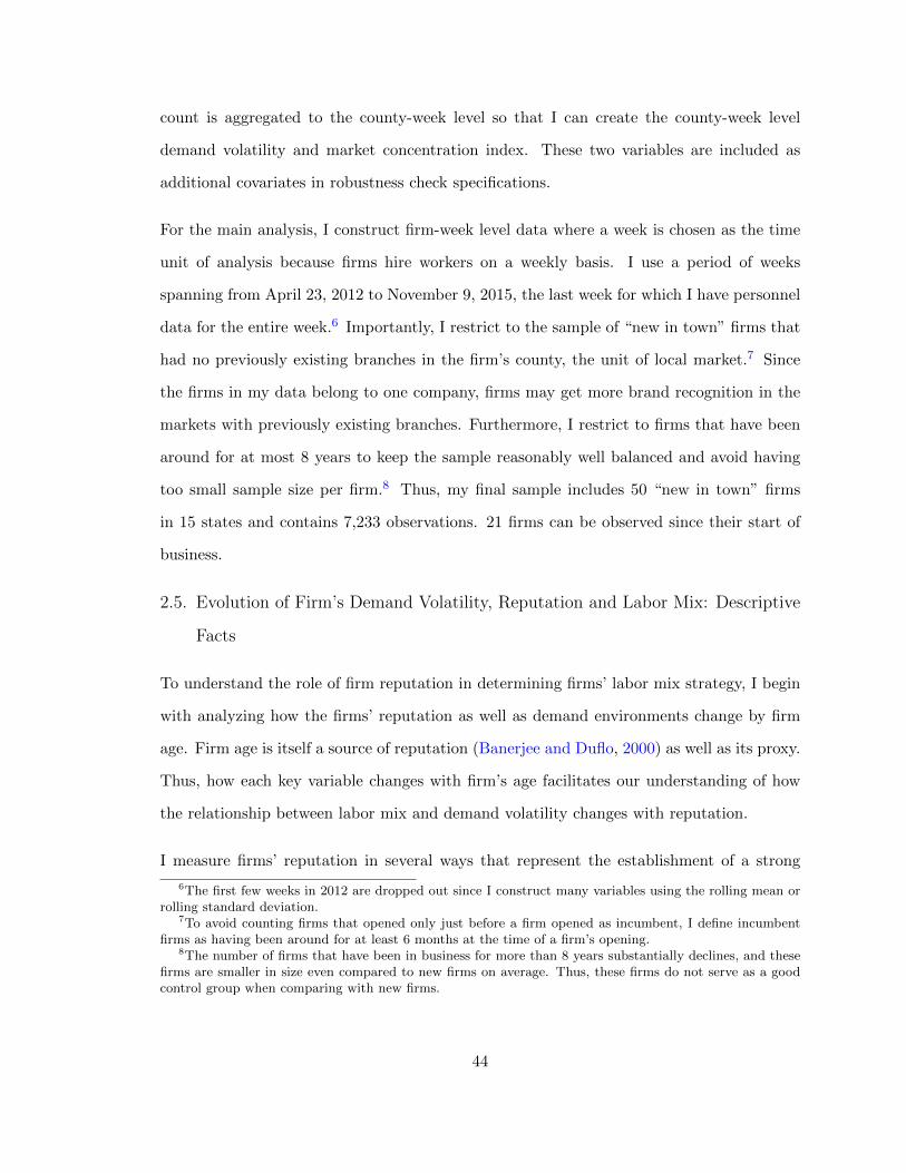
count is aggregated to the county-week level so that I can create the county-week level
demand volatility and market concentration index. These two variables are included as
additional covariates in robustness check specifications.
For the main analysis, I construct firm-week level data where a week is chosen as the time
unit of analysis because firms hire workers on a weekly basis. I use a period of weeks
spanning from April 23, 2012 to November 9, 2015, the last week for which I have personnel
data for the entire week.6 Importantly, I restrict to the sample of “new in town” firms that
had no previously existing branches in the firm’s county, the unit of local market.7 Since
the firms in my data belong to one company, firms may get more brand recognition in the
markets with previously existing branches. Furthermore, I restrict to firms that have been
around for at most 8 years to keep the sample reasonably well balanced and avoid having
too small sample size per firm.8 Thus, my final sample includes 50 “new in town” firms
in 15 states and contains 7,233 observations. 21 firms can be observed since their start of
business.
2.5. Evolution of Firm’s Demand Volatility, Reputation and Labor Mix: Descriptive
Facts
To understand the role of firm reputation in determining firms’ labor mix strategy, I begin
with analyzing how the firms’ reputation as well as demand environments change by firm
age. Firm age is itself a source of reputation (Banerjee and Duflo, 2000) as well as its proxy.
Thus, how each key variable changes with firm’s age facilitates our understanding of how
the relationship between labor mix and demand volatility changes with reputation.
I measure firms’ reputation in several ways that represent the establishment of a strong
6The first few weeks in 2012 are dropped out since I construct many variables using the rolling mean orrolling standard deviation.
7To avoid counting firms that opened only just before a firm opened as incumbent, I define incumbentfirms as having been around for at least 6 months at the time of a firm’s opening.
8The number of firms that have been in business for more than 8 years substantially declines, and thesefirms are smaller in size even compared to new firms on average. Thus, these firms do not serve as a goodcontrol group when comparing with new firms.
44

patient referral network, as referrals are the primary way of generating new demand. Par-
ticularly, I focus on the size of a referral network, and dispersion, consistency, and share of
referrals from hospitals. Hospitals are the largest referral source to home health agencies in
my data; hospital referrals account for 30% of new admissions a week on average.
For each firm i and week t, I create the following four measures of reputation Repit. Higher
value of reputation represents establishment of a stronger referral network. First, I measure
the size of a referral network by counting the number of unique hospital referral sources
that have referred to the firm i over the past 4 weeks including the current week, t´3, ..., t.
Second, I measure the dispersion of referrals, which equals minus 1 times the Herfindahl-
Hirschman index (HHI) of referrals among hospital referral sources over the previous 4
weeks. Thus, the higher and closer to zero the dispersion measure is, the more dispersed
referrals are. The more dispersed referral network represents a stronger network since a
firm does not depend on only a small set of hospitals to make referrals when the timing of
patient’s hospital discharge is idiosyncratic.
Third, I measure the consistency of referrals by computing the proportion of weeks a given
hospital j has referred to the home health firm i repeatedly in the previous 4 weeks. I
aggregate this firm-week-hospital level measure to the firm-week level by taking a weighted
average. For the hospital weight ωijt, I use the share of total hospital referrals received by i
over the past 4 weeks that come from each hospital j, assigning higher weights to hospitals
that have referred relatively more to the firm recently.
Fourth, I measure the firm’s share of referrals in each hospital, which represents the firm’s
importance as a referral partner to the hospitals. I compute the share of total Medicare
patients being discharged from a hospital j to home health over the past 4 weeks that are
referred to the home health firm i. This measures each firm i’s relative importance as a
referral partner to the hospital. Similar to the consistency measure above, I take a weighted
average of this firm-week-hospital level measure using the same weights ωijt.
45
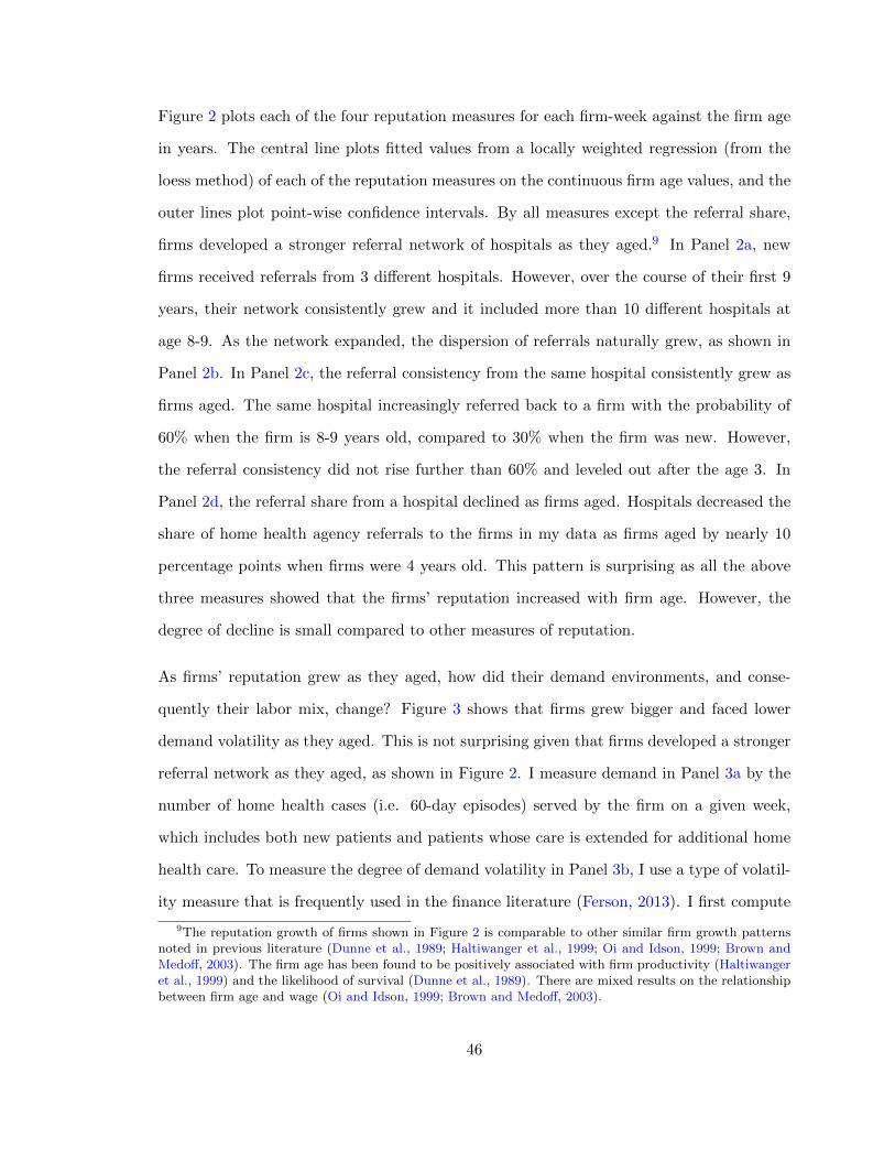
Figure 2 plots each of the four reputation measures for each firm-week against the firm age
in years. The central line plots fitted values from a locally weighted regression (from the
loess method) of each of the reputation measures on the continuous firm age values, and the
outer lines plot point-wise confidence intervals. By all measures except the referral share,
firms developed a stronger referral network of hospitals as they aged.9 In Panel 2a, new
firms received referrals from 3 different hospitals. However, over the course of their first 9
years, their network consistently grew and it included more than 10 different hospitals at
age 8-9. As the network expanded, the dispersion of referrals naturally grew, as shown in
Panel 2b. In Panel 2c, the referral consistency from the same hospital consistently grew as
firms aged. The same hospital increasingly referred back to a firm with the probability of
60% when the firm is 8-9 years old, compared to 30% when the firm was new. However,
the referral consistency did not rise further than 60% and leveled out after the age 3. In
Panel 2d, the referral share from a hospital declined as firms aged. Hospitals decreased the
share of home health agency referrals to the firms in my data as firms aged by nearly 10
percentage points when firms were 4 years old. This pattern is surprising as all the above
three measures showed that the firms’ reputation increased with firm age. However, the
degree of decline is small compared to other measures of reputation.
As firms’ reputation grew as they aged, how did their demand environments, and conse-
quently their labor mix, change? Figure 3 shows that firms grew bigger and faced lower
demand volatility as they aged. This is not surprising given that firms developed a stronger
referral network as they aged, as shown in Figure 2. I measure demand in Panel 3a by the
number of home health cases (i.e. 60-day episodes) served by the firm on a given week,
which includes both new patients and patients whose care is extended for additional home
health care. To measure the degree of demand volatility in Panel 3b, I use a type of volatil-
ity measure that is frequently used in the finance literature (Ferson, 2013). I first compute
9The reputation growth of firms shown in Figure 2 is comparable to other similar firm growth patternsnoted in previous literature (Dunne et al., 1989; Haltiwanger et al., 1999; Oi and Idson, 1999; Brown andMedoff, 2003). The firm age has been found to be positively associated with firm productivity (Haltiwangeret al., 1999) and the likelihood of survival (Dunne et al., 1989). There are mixed results on the relationshipbetween firm age and wage (Oi and Idson, 1999; Brown and Medoff, 2003).
46
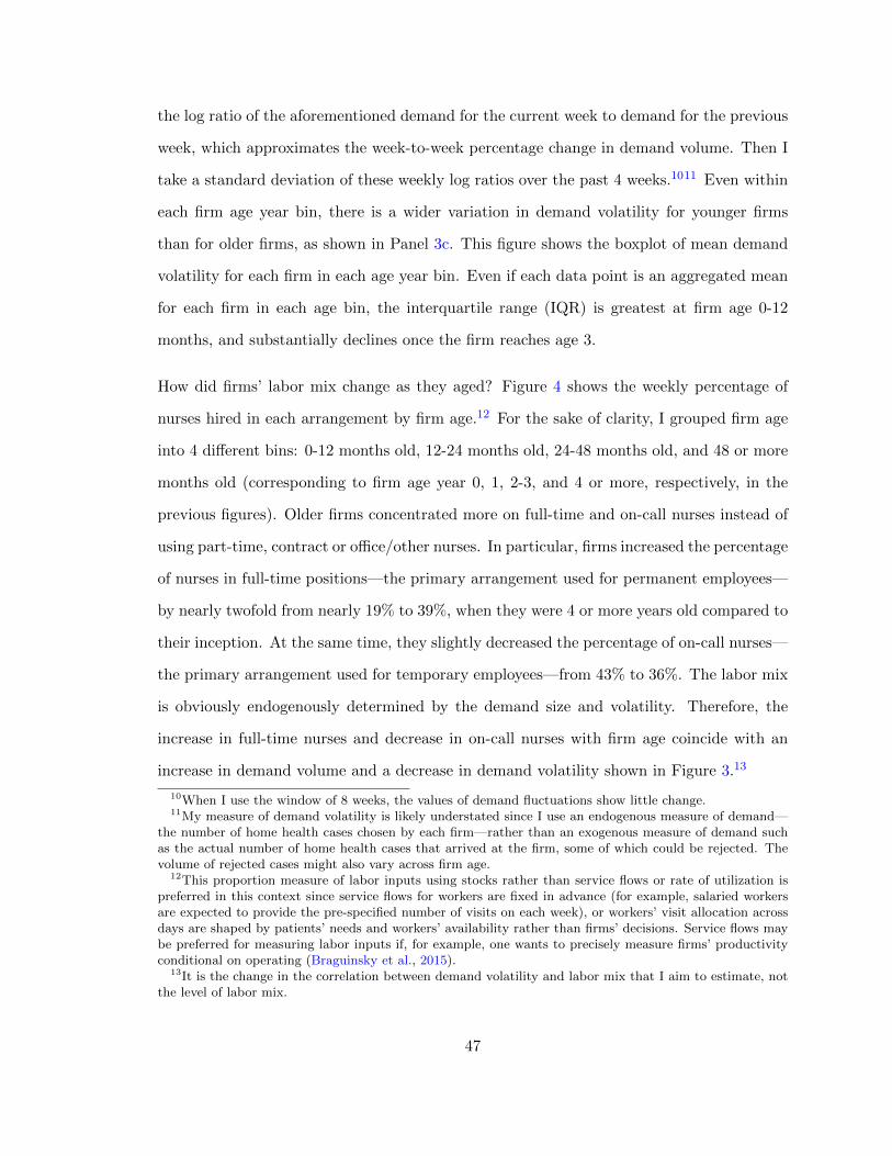
the log ratio of the aforementioned demand for the current week to demand for the previous
week, which approximates the week-to-week percentage change in demand volume. Then I
take a standard deviation of these weekly log ratios over the past 4 weeks.1011 Even within
each firm age year bin, there is a wider variation in demand volatility for younger firms
than for older firms, as shown in Panel 3c. This figure shows the boxplot of mean demand
volatility for each firm in each age year bin. Even if each data point is an aggregated mean
for each firm in each age bin, the interquartile range (IQR) is greatest at firm age 0-12
months, and substantially declines once the firm reaches age 3.
How did firms’ labor mix change as they aged? Figure 4 shows the weekly percentage of
nurses hired in each arrangement by firm age.12 For the sake of clarity, I grouped firm age
into 4 different bins: 0-12 months old, 12-24 months old, 24-48 months old, and 48 or more
months old (corresponding to firm age year 0, 1, 2-3, and 4 or more, respectively, in the
previous figures). Older firms concentrated more on full-time and on-call nurses instead of
using part-time, contract or office/other nurses. In particular, firms increased the percentage
of nurses in full-time positions—the primary arrangement used for permanent employees—
by nearly twofold from nearly 19% to 39%, when they were 4 or more years old compared to
their inception. At the same time, they slightly decreased the percentage of on-call nurses—
the primary arrangement used for temporary employees—from 43% to 36%. The labor mix
is obviously endogenously determined by the demand size and volatility. Therefore, the
increase in full-time nurses and decrease in on-call nurses with firm age coincide with an
increase in demand volume and a decrease in demand volatility shown in Figure 3.13
10When I use the window of 8 weeks, the values of demand fluctuations show little change.11My measure of demand volatility is likely understated since I use an endogenous measure of demand—
the number of home health cases chosen by each firm—rather than an exogenous measure of demand suchas the actual number of home health cases that arrived at the firm, some of which could be rejected. Thevolume of rejected cases might also vary across firm age.
12This proportion measure of labor inputs using stocks rather than service flows or rate of utilization ispreferred in this context since service flows for workers are fixed in advance (for example, salaried workersare expected to provide the pre-specified number of visits on each week), or workers’ visit allocation acrossdays are shaped by patients’ needs and workers’ availability rather than firms’ decisions. Service flows maybe preferred for measuring labor inputs if, for example, one wants to precisely measure firms’ productivityconditional on operating (Braguinsky et al., 2015).
13It is the change in the correlation between demand volatility and labor mix that I aim to estimate, notthe level of labor mix.
47
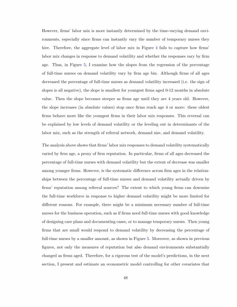
However, firms’ labor mix is more instantly determined by the time-varying demand envi-
ronments, especially since firms can instantly vary the number of temporary nurses they
hire. Therefore, the aggregate level of labor mix in Figure 4 fails to capture how firms’
labor mix changes in response to demand volatility and whether the responses vary by firm
age. Thus, in Figure 5, I examine how the slopes from the regression of the percentage
of full-time nurses on demand volatility vary by firm age bin. Although firms of all ages
decreased the percentage of full-time nurses as demand volatility increased (i.e. the sign of
slopes is all negative), the slope is smallest for youngest firms aged 0-12 months in absolute
value. Then the slope becomes steeper as firms age until they are 4 years old. However,
the slope increases (in absolute values) stop once firms reach age 4 or more: these oldest
firms behave more like the youngest firms in their labor mix responses. This reversal can
be explained by low levels of demand volatility or the leveling out in determinants of the
labor mix, such as the strength of referral network, demand size, and demand volatility.
The analysis above shows that firms’ labor mix responses to demand volatility systematically
varied by firm age, a proxy of firm reputation. In particular, firms of all ages decreased the
percentage of full-time nurses with demand volatility but the extent of decrease was smaller
among younger firms. However, is the systematic difference across firm ages in the relation-
ships between the percentage of full-time nurses and demand volatility actually driven by
firms’ reputation among referral sources? The extent to which young firms can downsize
the full-time workforce in response to higher demand volatility might be more limited for
different reasons. For example, there might be a minimum necessary number of full-time
nurses for the business operation, such as if firms need full-time nurses with good knowledge
of designing care plans and documenting cases, or to manage temporary nurses. Then young
firms that are small would respond to demand volatility by decreasing the percentage of
full-time nurses by a smaller amount, as shown in Figure 5. Moreover, as shown in previous
figures, not only the measures of reputation but also demand environments substantially
changed as firms aged. Therefore, for a rigorous test of the model’s predictions, in the next
section, I present and estimate an econometric model controlling for other covariates that
48

determine firms’ labor mix.
2.6. Empirical Analysis
2.6.1. Empirical Specification
Using the main specification below, I investigate how firms’ reputation among the referral
sources is related to firms’ labor mix responses to demand volatility. I look at changes in the
percentage of full-time nurses within a firm in response to an increase in demand volatility,
and use interaction terms between demand volatility and measures of firm reputation. The
estimating equations are of the form
yit “ β ` γ ¨DVit `DVit ¨Rep1it ¨ θ `Rep1it ¨ δ ` αi ` µt `X1it ¨ η ` εit, (2.20)
where yit is the percentage of active full-time nurses in firm i on week t. The key right-
hand-side variables are a measure of demand volatility, DVit, and interaction of the demand
volatility with a vector of different reputation measures, Repit, as described in Section 2.5.
Since I want to look at changes within firms, I include firm fixed effects αi, which allow
me to control for potential geography-specific market or legislative factors and differences
in time-constant management styles across firms. I also include week-year fixed effects µt
to control for any industry-wide shifts in or seasonal effects on the labor mix. In the vector
Xit, I include other firm-week level covariates, such as 7 indicators for firm age year bins
(omitted category is the indicator for the firm’s first year) or log firm age, log of total
demand volume, log of total active nursing workforce size, and the turnover rate among
full-time nurses.14
To facilitate the interpretation of interaction term coefficients, I nonparametrically estimate
the equation (2.20) using two quantile indicator variables for having 33-66th percentile
(“high”) values or 66-100th percentile (“very high”) values of each reputation measure
14The turnover rate is measured by a ratio of the number of full-time nurses leaving the workforce to thetotal number of active nurses for each firm-week.
49
(omitted category is the lowest quantile for smallest values). For each reputation measure,
I use quantile cutoffs based on the firm-specific distribution of all weeks within each one-year
firm age bin.15 The coefficients θ are identified from changes in the correlation between the
labor mix and demand volatility during weeks when a firm has particularly high reputation
given the firm age, compared to weeks when a firm has low reputation. The coefficients
θ will reflect how the correlations between the percentage of full-time nurses and demand
volatility change when each of different measures of reputation increases to “high” or “very
high” values. The key coefficient γ of our interest will reflect the correlation between
the percentage of full-time nurses and demand volatility when firms have low values of
reputation by all measures.
In Table 7, I provide summary statistics for the variables included in the regression.
2.6.2. Results on the Effects of Reputation on Firms’ Labor Mix Responses to Demand
Volatility
I investigate whether firms’ labor mix strategy in response to demand volatility systemat-
ically changes by their reputation among referral sources. Table 8 shows the results from
estimating the within-firm specification in (2.20) while controlling for a different combina-
tion of four reputation measures described in Section 2.5: 1) referral network size (i.e. the
total number of hospital referral sources); 2) dispersion of referrals; 3) referral consistency;
and 4) referral share (i.e. mean share of total home health referrals from each hospital).
Since the referral share data are available only for the years 2012–2014, specifications includ-
ing this reputation measure are estimated on this subsample. I begin with including only
one reputation measure at a time and include additional reputation measures to examine
whether firms respond differently to a change in different measures of reputation.
Table 8 shows consistently that firms’ percentage of full-time nurses was different when they
had low and high levels of reputation. When firms were in the bottom third of reputation
15I create different cutoffs for each firm age bin to adjust for different ranges in the reputation measuresacross firm ages, as shown in Figure 2, and allow for comparing the effects of reputation across firms ofsimilar tenure.
50

levels in the firm age-year specific distribution by any measures, they had a higher per-
centage of full-time nurses when demand volatility increased. In the first row, the positive
association between the percentage of full-time nurses and demand volatility is statistically
significant at the 5 percent level in all columns except columns (2) and (5). The correla-
tion tends to be particularly stronger when more than one reputation measure is included,
suggesting that different measures of reputation add up to each other in determining the
overall level of reputation from the firms’ perspective. Including a referral share using the
subsample period of 2012–2014 also yields stronger correlation. For example, when firms
had only a small referral network, the coefficient on demand volatility is 20.89 in column
(1). But when firms had both small referral network and low referral consistency in column
(6), the coefficient on demand volatility increases to 27.55. The coefficient declines slightly
to 25.47 when firms also had low referral dispersion on top of these two variables in col-
umn (11) but rises again to 33.97 when firms also received a low referral share in column
(13). The magnitudes implied by the coefficients are small, however, since demand volatility
ranges from 0 to around 1. Firms with low reputation by all measures hired about 0.8-1.4
percentage-point or 2-4 percent more full-time nurses when demand volatility increased by
one standard deviation (0.04).16 This is translated to 0.2 to 0.3 more full-time nurse in an
average firm that hired 21 nurses per week in total.
On the other hand, firms had a lower percentage of full-time nurses when reputation in-
creased by any one of the measures, as shown by the negative coefficients on interaction
terms. The negative coefficients on interaction terms are usually statistically significant
only when reputation was higher in terms of referral network size and referral consistency,
and are more likely to be significant for the top quantile indicators for each of the repu-
tation measures. When firms had a top third size of referral network in the firm age-year
specific distribution in column (1), the positive association between the percentage of full-
time nurses and demand volatility is canceled out. When firms had a very large referral
162-4 percent increase is obtained by multiplying the estimated coefficients by the standard deviation ofdemand volatility, 0.04, times 100, divided by the mean percentage of full-time nurses, 34 percent.
51

network but had low referral consistency and received a low referral share in column (13),
the percentage of full-time nurses was 2 percent higher when demand volatility increased by
one standard deviation, as opposed to 4 percent higher when firms also had a small referral
network. However, the positive association is canceled out again when firms had both a
very large network and very high referral consistency even though firms still received a low
referral share.
The main results from the above show that firms with lower reputation than expected for
those in the firm age-year hired more full-time nurses in response to higher demand volatility
than firms with higher reputation. However, did younger firms behave differently from older
firms? Figure 2 shows that reputation increased with firm age. Do the results in Table 8
hold regardless of firm age and levels of reputation? The theory in Section 2.3 predicts that
firms with lower levels of reputation—i.e. younger firms—increase the percentage of full-
time nurses by even more than firms with higher levels of reputation. To investigate this,
I separately estimate the equation (2.20) for firms in different age bins. I divide firm-week
observations into three groups by firm age: 1) firms aged 0–12 months; 2) firms aged 12–48
months; and 3) firms aged 48 or more months. I replace the firm age year indicators with a
continuous log firm age variable. Findings in Table 8 suggest that referral network size and
referral consistency are measures of reputation to which firms were most sensitive. Thus,
I focus on the specifications with these two measures of reputation in the next analyses.
The full sample also ensures a large sample size for statistical power while the results were
qualitatively similar, and yields rather conservative estimates.
In Table 9, it is only the youngest firms aged 0–12 months in columns (1)–(3) that had
statistically significant positive associations between the percentage of full-time nurses and
demand volatility when firms had a small referral network and low referral consistency.
When demand volatility increased by one standard deviation (0.08), young firms with a
small referral network had a 4 percentage-point or 17 percent higher percentage of full-time
nurses compared to the mean percentage of full-time nurses at 25.62 percent according to
52
column (1). From column (2), young firms with low referral consistency had a 6 percentage-
point or 23 percent higher percentage of full-time nurses. From column (3), young firms
with both small referral network and low referral consistency also had a 6 percentage-point
or 24 percent higher percentage of full-time nurses. These results suggest having around
0.5-1 more full-time nurses given the mean total workforce size of 13 nurses among these
young firms.
For older firms aged 12–48 months or more than 48 months, they had positive associa-
tions between the percentage of full-time nurses and demand volatility when having the
bottom third of a reputation distribution. However, these associations are not statistically
significant at the 10 percent level.
Moreover, it is only the youngest firms aged 0–12 months that had a statistically significant
negative interaction term with a reputation measure, and the significant association appears
only when the reputation is measured by referral consistency in columns (2) and (3). Column
(2) shows that when young firms had high referral consistency, they had a 6 percent higher
percentage of full-time nurses, as opposed to 23 percent, when demand volatility increased
by one standard deviation. When young firms had very high referral consistency, they even
had a slightly lower percentage of full-time nurses by 0.7 percent when demand volatility
increased by one standard deviation. In comparison, results for older firms show that
interaction coefficients have opposite signs and also are not precisely estimated even though
the sample sizes are greater. Reputation may not be the most important driver of firms’
labor mix responses for these older firms. Thus, findings in Table 8 are primarily driven by
young firms in my data, which reinforce my model’s predictions.
How did firms adjust their nursing workforce hired in other employment arrangements be-
yond full-time nurses? Since the percentage of nurses in each work arrangement sums up to
100 percent, an increase in the percentage of full-time nurses must accompany a decrease in
the percentage of other nurses when firms had low reputation. However, which other work
arrangement did firms adjust the most when they had low reputation? Did they differen-
53

tially treat directly hired on-call nurses and independently contracted nurses? I investigate
firms’ heterogeneous responses to demand volatility across work arrangements. I estimate
the equation (2.20) among the youngest firms aged 0–12 months using the percentage of ac-
tive nurses hired in each arrangement as the dependent variable. For reputation measures,
I include both referral network size and referral consistency.
In Table 10, I present columns in a descending order of organizational attachment of the
arrangements (except the “Office/Other” category in column (6) representing office or other
employees whose primary duty is not to visit patients). Column (1) reports the same results
as in column (3) of Table 9 for full-time nurses while columns (2)–(6) show the results for
nurses hired in part-time with benefits, part-time without benefits, on-call, independent
contractor, and office/other categories. In the first row, firms in the bottom third of both
reputation distributions during the first year had a lower percentage of nurses in all positions
except in full-time positions. However, the only statistically significant negative association
appears for independently contracted nurses, who have the least organizational attachment,
in column (5). When having both small referral network and low referral consistency, young
firms had a 4 percentage-point or 28% lower percentage of contractor nurses when demand
volatility increased by one standard deviation. This translates to hiring 0.5 fewer contractor
nurses.
Other statistically significant labor mix responses are using more part-time nurses with
benefits when firms had higher referral consistency despite having a small referral network;
however, firms used fewer part-time nurses when having a very large referral network if they
had low referral consistency. Moreover, firms used fewer office/other nurses when having
a larger referral network if they had low referral consistency. These results suggest that
firms did not view part-time nurses with benefits or office nurses as substitutes for full-time
nurses. Furthermore, firms appear more sensitive to referral consistency as a measure of
reputation, as indicated earlier.
54
2.7. Alternative Explanations and Robustness Checks
2.7.1. Refuting the Alternative Explanation by Firm Size
The above findings are consistent with my model’s predictions that reputation changes
firms’ labor mix responses to demand volatility. Firms with lower reputation had a higher
percentage of full-time nurses when demand volatility increased. However, firms with higher
reputation had either no change in or even a lower percentage of full-time nurses when
demand volatility increased. These results are driven by youngest firms aged 0–12 months
which also had the lowest reputation by any measures. Furthermore, low-reputation firms
simultaneously decreased the percentage of contractor nurses with demand volatility.
However, there is a potential concern that the effect of reputation found above could be
driven by other factors. A plausible confounding factor is the firm size. Section 2.5 showed
that younger firms not only had lower reputation but also were smaller on average. Smaller
young firms may expect to grow in the future more rapidly. There could be unobserved
information about their formation of relationships with more referral sources, which I cannot
control for. If so, firms with lower reputation could be the small ones with greater expected
growth which, simultaneously, would increase the percentage of full-time nurses. Moreover,
smaller firms plausibly incur higher costs of attracting temporary nurses. They face higher
demand volatility, which could create more unstable work schedules for temporary nurses.
Smaller firms also may be capacity constrained and have a shortage of human resources staff
who play an important role in recruiting temporary workers. If these were the cases, then
young firms could respond to demand volatility by increasing full-time or other permanent
nurses purely due to a smaller size. I control for contemporaneous demand and nursing
workforce sizes on the right-hand side when estimating (2.20). However, to the extent that
firms have unobserved information on the demand growth forecast and hiring costs, the
coefficients γ on demand volatility and θ on the interaction terms could be contaminated
by the omitted variable bias.
55
To disentangle the role of reputation among referral sources from the effect of firm size, I
indirectly test whether the effects of reputation among young firms in Table 9 are driven by
small young firms or large young firms. If it is large young firms that drive the results, then
I can rule out the alternative explanation by the firm size. In Table 11 I report the results
from estimating (2.20) separately for small and large young firms in each firm age group
shown in Table 9. Large firms are defined as those in each firm age year bin having their
mean total demand volume during the age year above the median.17 I include the referral
network size and referral consistency as reputation measures.
In the first row, it is only the young large firms aged 0–12 months in column (2) that had a
positive association between the percentage of full-time nurses and demand volatility when
firms had both small referral network and low referral consistency. While the coefficient is
positive for both small and large young firms, it nearly doubles in size and is statistically
significant only for large young firms. When large young firms had both small referral
network and low referral consistency, they had a 4 percentage-point or 14 percent higher
percentage of full-time nurses when demand volatility increased by one standard deviation
(0.05), compared to the mean percentage of full-time nurses at 27 percent. This translates
to 0.6 more full-time nurses given the mean nursing workforce size of 16 nurses in these
firms. However, when these firms had larger referral network or higher referral consistency,
the association between the percentage of full-time nurses and demand volatility is posi-
tive and negative, respectively, and not statistically significant at the 10% level. Thus, it
appears that large young firms increased the percentage of full-time nurses with demand
volatility, regardless of their reputation levels. In summary, columns (1) and (2) show that
the reputation effects I am capturing for young firms are not driven by the firm size effects.
Similarly, I examine whether small and large firms among older firms behaved differently
from each other in columns (3)–(6). Although I do not find any statistically significant
effects among old firms in Table 9, the effects might differ by the firm size. The oldest
17I define whether a firm is large separately for each firm age year bin since firms’ size varies by age. Thus,one firm can be large in one age year and small in another age year.
56

firms, aged 48 or more months, seem to respond to demand volatility differently according
to the size of referral network in columns (5) and (6) but these interaction terms are only
weakly statistically significant.
2.7.2. Falsificateion Test by Comparing with “Not New in Town” Firms
I provide further evidence that firms’ reputation among referral sources determines their
labor mix responses to demand volatility by conducting a falsification test. In this test, I
compare “new in town” firms, which have been my main sample for preceding analysis, with
“not new in town” firms, defined as those that had previously existing branches in thecounty,
the unit of a local market.18 I expect to find no effects of reputation among “not new in
town” firms since they would be less sensitive to the levels of reputation among referral
sources. They can get more brand recognition through previously established branch firms
and be more likely to be receive referrals even without improving quality (i.e. “piggybacking
effect”). This effect would lead to a particularly salient difference in firms’ labor mix when
firms have low reputation. “Not new in town” firms would not necessarily have to increase
the percentage of full-time nurses with demand volatility.
This falsification test might be ineffective to the extent that low-reputation firms in mar-
kets with previously existing branch firms try to internalize the reputation externality (i.e.
“reputation externality” effect) (Jin and Leslie, 2009). “Not new in town” firms may be
more concerned about keeping up the high quality level if the consequence of low quality
signals is transmitted to the other firms in the same market. This concern will be greater
in markets with more existing branch firms. If this effect prevails, “not new in town” firms
could behave just like “new in town” firms.
To empirically test for the piggybacking effect and reputation externality effect, I reestimate
(2.20) using the sample of all “not new in town” firms and report results in column (1) of
18It is possible to use different units of markets at different scopes—Hospital Referral Regions (HRRs),which define larger market areas, and Hospital Service Areas (HSAs), which define smaller market areasthan counties. However, an HRR is too large, leaving too few firms that are new in the area. On the otherhand, an HSA is too small and a firm’s set of patients are usually contained in multiple HSAs, rendering itinappropriate as a local market for referrals from hospitals.
57
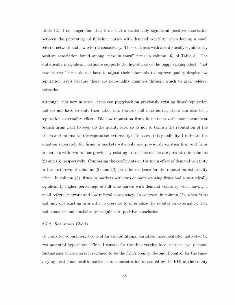
Table 12. I no longer find that firms had a statistically significant positive association
between the percentage of full-time nurses with demand volatility when having a small
referral network and low referral consistency. This contrasts with a statistically significantly
positive association found among “new in town” firms in column (6) of Table 8. The
statistically insignificant estimate supports the hypothesis of the piggybacking effect: “not
new in town” firms do not have to adjust their labor mix to improve quality despite low
reputation levels because there are non-quality channels through which to grow referral
networks.
Although “not new in town” firms can piggyback on previously existing firms’ reputation
and do not have to shift their labor mix towards full-time nurses, there can also be a
reputation externality effect. Did low-reputation firms in markets with more incumbent
branch firms want to keep up the quality level so as not to tarnish the reputation of the
others and internalize the reputation externality? To assess this possibility, I estimate the
equation separately for firms in markets with only one previously existing firm and firms
in markets with two to four previously existing firms. The results are presented in columns
(2) and (3), respectively. Comparing the coefficients on the main effect of demand volatility
in the first rows of columns (2) and (3) provides evidence for the reputation externality
effect. In column (3), firms in markets with two or more existing firms had a statistically
significantly higher percentage of full-time nurses with demand volatility when having a
small referral network and low referral consistency. In contrast, in column (2), when firms
had only one existing firm with no pressure to internalize the reputation externality, they
had a smaller and statistically insignificant, positive association.
2.7.3. Robustness Checks
To check for robustness, I control for two additional variables incrementally, motivated by
two potential hypotheses. First, I control for the time-varying local market-level demand
fluctuations where market is defined to be the firm’s county. Second, I control for the time-
varying local home health market share concentration measured by the HHI at the county
58
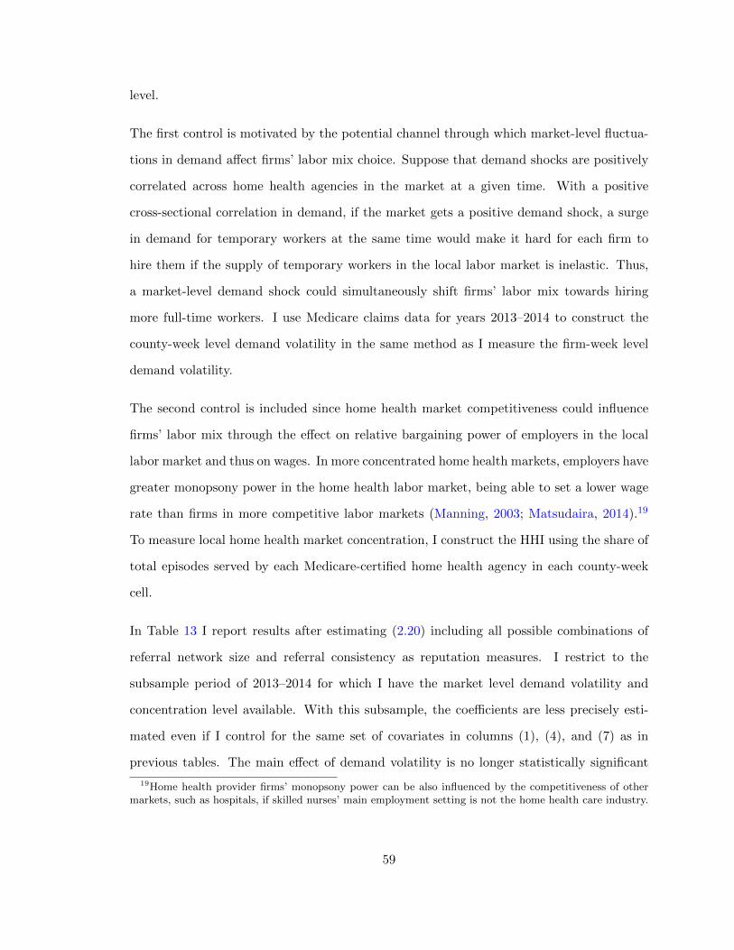
level.
The first control is motivated by the potential channel through which market-level fluctua-
tions in demand affect firms’ labor mix choice. Suppose that demand shocks are positively
correlated across home health agencies in the market at a given time. With a positive
cross-sectional correlation in demand, if the market gets a positive demand shock, a surge
in demand for temporary workers at the same time would make it hard for each firm to
hire them if the supply of temporary workers in the local labor market is inelastic. Thus,
a market-level demand shock could simultaneously shift firms’ labor mix towards hiring
more full-time workers. I use Medicare claims data for years 2013–2014 to construct the
county-week level demand volatility in the same method as I measure the firm-week level
demand volatility.
The second control is included since home health market competitiveness could influence
firms’ labor mix through the effect on relative bargaining power of employers in the local
labor market and thus on wages. In more concentrated home health markets, employers have
greater monopsony power in the home health labor market, being able to set a lower wage
rate than firms in more competitive labor markets (Manning, 2003; Matsudaira, 2014).19
To measure local home health market concentration, I construct the HHI using the share of
total episodes served by each Medicare-certified home health agency in each county-week
cell.
In Table 13 I report results after estimating (2.20) including all possible combinations of
referral network size and referral consistency as reputation measures. I restrict to the
subsample period of 2013–2014 for which I have the market level demand volatility and
concentration level available. With this subsample, the coefficients are less precisely esti-
mated even if I control for the same set of covariates in columns (1), (4), and (7) as in
previous tables. The main effect of demand volatility is no longer statistically significant
19Home health provider firms’ monopsony power can be also influenced by the competitiveness of othermarkets, such as hospitals, if skilled nurses’ main employment setting is not the home health care industry.
59
except in columns (1)–(3) when firms had a small referral network. However, it is reassuring
that the results change little once additional controls—market-level demand volatility and
market concentration—are included.
2.8. Conclusion
This chapter demonstrates that firms’ reputation is an important determinant of labor
mix in the face of demand fluctuations. I find that firms with lower reputation, especially
younger firms, employ larger percentages of full-time nurses. This suggests that firms forgo
short-term profitability in order to achieve long-term reputation through improvements in
service quality. This hypothesis is further supported by evidence from Chapter 1 that
patients visited by a higher proportion of full-time nurses were less likely to have a hospital
readmission.
These observations have important implications for both industry and policy. First, for
industry, this chapter shows that starting firms strategically adjust their labor mix in order
to grow their reputation for quality and increase their referral base. Whether this is optimal
for businesses and society would require a further examination of the endogenous increases
in referral volume and improvement quality as a result of the firms’ behaviors. This will
be a fruitful avenue for future research. Second, although the home health market has
been widely viewed as having low barriers to entry due to low capital requirements, this
chapter points to a new barrier to entry since starting firms have to employ a higher share
of permanent labor than more established firms.
60

Figure 2: Measures of Reputation by Firm Age
(a) Size of referral network (b) Dispersion of referrals
(c) Consistency of referrals (d) Share of referrals from each hospital
Notes: In each panel, the lines plot fitted values, along with point-wise 95-percent confidence intervals, oflocally weighted regressions (using R’s ggplot command with a geom smooth option) of each reputationmeasure on firm age in years at the firm-week level. The size of referral network in Panel (a) is measuredby the number of unique hospital referral sources that has referred to a home health firm in the past 4weeks, including the current week. The dispersion of referrals in Panel (b) is measured by minus 1 timesthe Herfindahl-Hirschman index (HHI) of referrals in the past 4 weeks. The consistency of referrals in Panel(c) is measured by the percentage of weeks referred by the same hospital referral source in the past 4 weeks.The share of referrals from each hospital in Panel (d) is measured by the percentage of home health referralsfrom a hospital made to the firm, aggregated across hospitals.
61
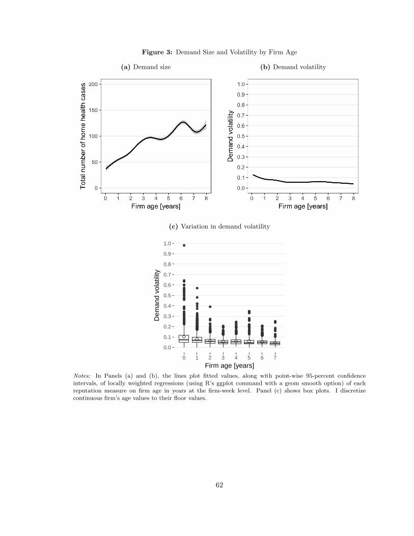
Figure 3: Demand Size and Volatility by Firm Age
(a) Demand size (b) Demand volatility
(c) Variation in demand volatility
●●●
●
●
●●●
●
●
●
●
●●
●
●●●
●●●
●●
●
●●●
●●
●
●
●
●
●●
●●●●●●
●●●
●●
●●●●
●●●●
●●
●●
●
●
●
●
●
●
●
●
●
●●
●●
●●
●
●
●●
●
●●
●●●
●●●●
●●●●
●●
●●●●
●●
●●●●●
●
●●●
●
●●●
●
●●●
●●●●
●●●●●●
●
●
●●●●●●●●
●
●
●●
●●
●●●●●
●●●
●
●●●●●●●
●
●●●●●●
●●●●●●●●●
●●●
●
●●●●
●●●●●●●●●●●●●●●●●
●●●●●
●●
●●●●●●●●●
●
●●
●●●
●
●●●●
●●●
●
●●●
●
●●●●
●●●●
●
●●●●●
●●●
●
●●●●
●●
●
●
●
●●●
●●
●●
●●●●●
●
●●
●●
●●●●●●●●
●●●●●●
●●●●●●●●●●● ●●
●●
●●●●
●●●
●●
●
0.0
0.1
0.2
0.3
0.4
0.5
0.6
0.7
0.8
0.9
1.0
0 1 2 3 4 5 6 7
Firm age [years]
Dem
and
vola
tility
Notes: In Panels (a) and (b), the lines plot fitted values, along with point-wise 95-percent confidenceintervals, of locally weighted regressions (using R’s ggplot command with a geom smooth option) of eachreputation measure on firm age in years at the firm-week level. Panel (c) shows box plots. I discretizecontinuous firm’s age values to their floor values.
62

Figure 4: Labor Mix by Firm Age Bin
18.9
43.4
71.610.3
18.8
25
40.3
10.21.76.3
16.6
30.3
39.7
10.5
34.5
12.1
38.9
36
8.1
4.64.3
8.1
0
20
40
60
80
100
0−12 mo 12−24 mo 24−48 mo 48+ mo
Firm age
Mea
n pe
rcen
tage
of a
ctiv
e nu
rses
Office/Other
Contractor
Part−time w/o benefits
Part−time w/ benefits
On−call
Full−time
Notes: Weekly values for each variable are averaged in each firm’s age bin for each firm.
63
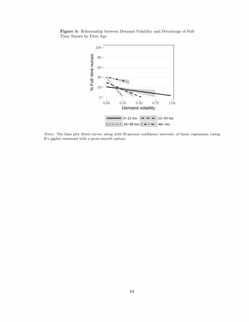
Figure 5: Relationship between Demand Volatility and Percentage of Full-Time Nurses by Firm Age
0
20
40
60
80
100
0.00 0.25 0.50 0.75 1.00
Demand volatility
% F
ull−
time
nurs
es
0−12 mo 12−24 mo
24−48 mo 48+ mo
Notes: The lines plot fitted curves, along with 95-percent confidence intervals, of linear regressions (usingR’s ggplot command with a geom smooth option)
64
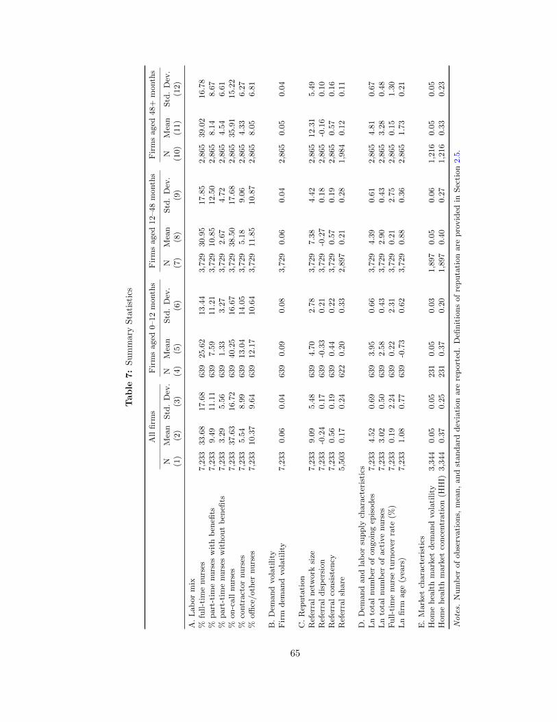
Table
7:
Su
mm
ary
Sta
tist
ics
All
firm
sF
irm
saged
0–12
month
sF
irm
saged
12–48
month
sF
irm
saged
48+
month
s
NM
ean
Std
.D
ev.
NM
ean
Std
.D
ev.
NM
ean
Std
.D
ev.
NM
ean
Std
.D
ev.
(1)
(2)
(3)
(4)
(5)
(6)
(7)
(8)
(9)
(10)
(11)
(12)
A.
Lab
or
mix
%fu
ll-t
ime
nurs
es7,2
33
33.6
817.6
8639
25.6
213.4
43,7
29
30.9
517.8
52,8
65
39.0
216.7
8%
part
-tim
enurs
esw
ith
ben
efits
7,2
33
9.4
911.1
1639
7.5
911.2
13,7
29
10.8
512.5
02,8
65
8.1
48.6
7%
part
-tim
enurs
esw
ithout
ben
efits
7,2
33
3.2
95.5
6639
1.3
33.2
73,7
29
2.6
74.7
22,8
65
4.5
46.6
1%
on-c
all
nurs
es7,2
33
37.6
316.7
2639
40.2
516.6
73,7
29
38.5
017.6
82,8
65
35.9
115.2
2%
contr
act
or
nurs
es7,2
33
5.5
48.9
9639
13.0
414.0
53,7
29
5.1
89.0
62,8
65
4.3
36.2
7%
offi
ce/oth
ernurs
es7,2
33
10.3
79.6
4639
12.1
710.6
43,7
29
11.8
510.8
72,8
65
8.0
56.8
1
B.
Dem
and
vola
tility
Fir
mdem
and
vola
tility
7,2
33
0.0
60.0
4639
0.0
90.0
83,7
29
0.0
60.0
42,8
65
0.0
50.0
4
C.
Rep
uta
tion
Ref
erra
lnet
work
size
7,2
33
9.0
95.4
8639
4.7
02.7
83,7
29
7.3
84.4
22,8
65
12.3
15.4
9R
efer
ral
dis
per
sion
7,2
33
-0.2
40.1
7639
-0.3
30.2
13,7
29
-0.2
70.1
82,8
65
-0.1
60.1
0R
efer
ral
consi
sten
cy7,2
33
0.5
60.1
9639
0.4
40.2
23,7
29
0.5
70.1
92,8
65
0.5
70.1
6R
efer
ral
share
5,5
03
0.1
70.2
4622
0.2
00.3
32,8
97
0.2
10.2
81,9
84
0.1
20.1
1
D.
Dem
and
and
lab
or
supply
chara
cter
isti
csL
nto
tal
num
ber
of
ongoin
gep
isodes
7,2
33
4.5
20.6
9639
3.9
50.6
63,7
29
4.3
90.6
12,8
65
4.8
10.6
7L
nto
tal
num
ber
of
act
ive
nurs
es7,2
33
3.0
20.5
0639
2.5
80.4
33,7
29
2.9
00.4
32,8
65
3.2
80.4
8F
ull-t
ime
nurs
etu
rnov
erra
te(%
)7,2
33
0.1
92.2
4639
0.2
22.3
13,7
29
0.2
12.7
52,8
65
0.1
51.3
0L
nfirm
age
(yea
rs)
7,2
33
1.0
80.7
7639
-0.7
30.6
23,7
29
0.8
80.3
62,8
65
1.7
30.2
1
E.
Mark
etch
ara
cter
isti
csH
om
ehea
lth
mark
etdem
and
vola
tility
3,3
44
0.0
50.0
5231
0.0
50.0
31,8
97
0.0
50.0
61,2
16
0.0
50.0
5H
om
ehea
lth
mark
etco
nce
ntr
ati
on
(HH
I)3,3
44
0.3
70.2
5231
0.3
70.2
01,8
97
0.4
00.2
71,2
16
0.3
30.2
3
Notes.
Num
ber
of
obse
rvati
ons,
mea
n,
and
standard
dev
iati
on
are
rep
ort
ed.
Defi
nit
ions
of
reputa
tion
are
pro
vid
edin
Sec
tion
2.5
.
65
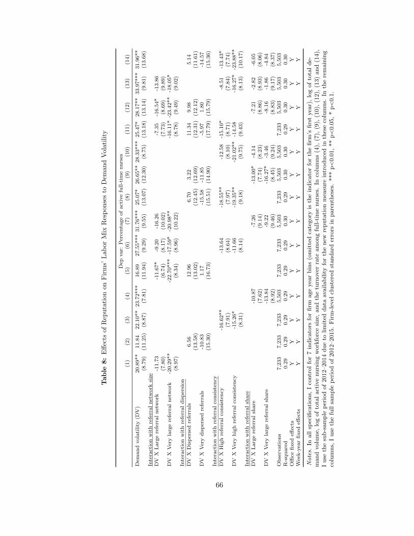
Table
8:
Eff
ects
of
Rep
uta
tion
on
Fir
ms’
Lab
or
Mix
Res
pon
ses
toD
eman
dV
ola
tility
Dep
var:
Per
centa
ge
of
act
ive
full-t
ime
nu
rses
(1)
(2)
(3)
(4)
(5)
(6)
(7)
(8)
(9)
(10)
(11)
(12)
(13)
(14)
Dem
an
dvola
tility
(DV
)20.8
9**
11.8
422.1
0**
23.7
2***
16.8
927.5
5***
31.7
6***
25.0
7*
26.6
5**
28.3
3***
25.4
7*
28.1
7**
33.9
7***
31.9
6**
(8.7
9)
(11.2
5)
(8.8
7)
(7.8
1)
(11.9
4)
(9.2
9)
(9.5
5)
(13.0
7)
(12.3
0)
(8.7
5)
(13.1
8)
(13.1
4)
(9.8
1)
(13.6
8)
Inte
ract
ion
wit
hre
ferr
al
net
work
size
DV
XL
arg
ere
ferr
al
net
work
-11.7
3-1
1.6
7*
-9.2
0-1
6.2
6-7
.35
-16.5
4*
-13.8
6(7
.80)
(6.7
4)
(8.1
7)
(10.0
2)
(7.7
3)
(8.6
9)
(9.8
9)
DV
XV
ery
larg
ere
ferr
al
net
work
-20.2
9**
-22.7
0***
-17.5
9*
-20.9
8**
-16.1
1*
-23.4
2**
-18.0
5*
(8.9
7)
(8.3
4)
(8.9
6)
(10.2
2)
(8.7
8)
(9.4
9)
(9.0
2)
Inte
ract
ion
wit
hre
ferr
al
dis
per
sion
DV
XD
isp
erse
dre
ferr
als
6.5
612.9
66.7
03.2
211.3
49.9
85.1
4(1
3.5
8)
(13.0
2)
(12.4
5)
(12.6
9)
(12.3
1)
(12.1
2)
(11.6
1)
DV
XV
ery
dis
per
sed
refe
rrals
-10.8
31.1
7-1
5.5
8-1
1.8
5-5
.97
1.8
0-1
4.5
7(1
5.3
0)
(16.7
3)
(15.5
1)
(14.9
0)
(17.7
9)
(15.7
9)
(15.3
6)
Inte
ract
ion
wit
hre
ferr
al
con
sist
ency
DV
XH
igh
refe
rral
con
sist
ency
-16.6
2**
-13.6
4-1
8.5
5**
-12.5
8-1
5.1
0*
-8.5
1-1
3.4
3*
(7.9
1)
(8.6
4)
(7.9
7)
(8.1
0)
(8.7
1)
(7.8
4)
(7.7
4)
DV
XV
ery
hig
hre
ferr
al
con
sist
ency
-15.2
6*
-11.6
6-1
9.3
5**
-21.0
2**
-14.5
8-1
6.2
7*
-23.8
8**
(8.3
1)
(8.1
4)
(9.1
8)
(9.7
5)
(9.4
3)
(8.1
3)
(10.1
7)
Inte
ract
ion
wit
hre
ferr
al
share
DV
XL
arg
ere
ferr
al
share
-10.8
7-7
.26
-13.0
0*
-4.1
4-7
.21
-2.8
2-6
.05
(7.6
2)
(9.1
4)
(7.7
4)
(8.2
3)
(8.8
6)
(8.9
3)
(8.0
6)
DV
XV
ery
larg
ere
ferr
al
share
-13.8
4-9
.22
-16.2
7*
-3.4
6-8
.16
-1.8
6-4
.84
(8.9
2)
(9.4
6)
(8.4
5)
(9.2
4)
(8.8
3)
(9.1
7)
(8.3
7)
Ob
serv
ati
on
s7,2
33
7,2
33
7,2
33
5,5
03
7,2
33
7,2
33
5,5
03
7,2
33
5,5
03
5,5
03
7,2
33
5,5
03
5,5
03
5,5
03
R-s
qu
are
d0.2
90.2
90.2
90.2
90.2
90.2
90.3
00.2
90.3
00.3
00.2
90.3
00.3
00.3
0O
ffice
fixed
effec
tsY
YY
YY
YY
YY
YY
YY
YW
eek-y
ear
fixed
effec
tsY
YY
YY
YY
YY
YY
YY
Y
Notes.
Inall
spec
ifica
tions,
Ico
ntr
ol
for
7in
dic
ato
rsfo
rfirm
age
yea
rbin
s(o
mit
ted
cate
gory
isth
ein
dic
ato
rfo
rth
efirm
’sfirs
tyea
r),
log
of
tota
lde-
mand
volu
me,
log
of
tota
lact
ive
nurs
ing
work
forc
esi
ze,
and
the
turn
over
rate
am
ong
full-t
ime
nurs
es.
Inco
lum
ns
(4),
(7),
(9),
(10),
(12),
(13)
and
(14),
Iuse
the
sub-s
am
ple
per
iod
of
2012–2014
due
tolim
ited
data
availabilit
yfo
rth
enew
reputa
tion
mea
sure
intr
oduce
din
thes
eco
lum
ns.
Inth
ere
main
ing
colu
mns,
Iuse
the
full
sam
ple
per
iod
of
2012–2015.
Fir
m-l
evel
clust
ered
standard
erro
rsin
pare
nth
eses
.***
pă
0.0
1,
**
pă
0.0
5,
*p
ă0.1
.
66
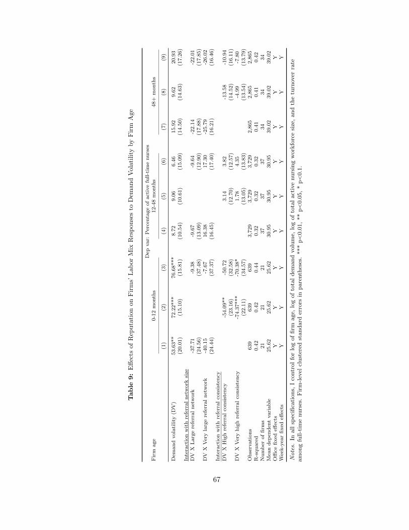
Table
9:
Eff
ects
ofR
epu
tati
on
on
Fir
ms’
Lab
or
Mix
Res
pon
ses
toD
eman
dV
ola
tili
tyby
Fir
mA
ge
Dep
var:
Per
centa
ge
of
act
ive
full-t
ime
nu
rses
Fir
mage
0-1
2m
onth
s12-4
8m
onth
s48+
month
s
(1)
(2)
(3)
(4)
(5)
(6)
(7)
(8)
(9)
Dem
an
dvola
tility
(DV
)53.6
3**
72.2
2***
76.6
8***
8.7
29.0
66.4
615.9
29.6
220.9
3(2
0.0
1)
(15.1
0)
(15.8
1)
(10.5
4)
(10.6
1)
(15.0
9)
(14.5
0)
(14.6
3)
(17.2
6)
Inte
ract
ion
wit
hre
ferr
al
net
work
size
DV
XL
arg
ere
ferr
al
net
work
-37.7
1-9
.38
-9.6
7-9
.64
-22.1
4-2
2.0
1(2
4.5
6)
(37.4
8)
(13.0
9)
(12.9
0)
(17.8
8)
(17.8
5)
DV
XV
ery
larg
ere
ferr
al
net
work
-40.1
5-7
.67
16.3
817.3
0-2
5.7
9-2
6.0
2(2
4.4
4)
(37.3
7)
(16.4
5)
(17.4
0)
(16.2
1)
(16.4
6)
Inte
ract
ion
wit
hre
ferr
al
con
sist
ency
DV
XH
igh
refe
rral
con
sist
ency
-54.0
9**
-50.7
23.1
43.8
2-1
3.5
8-1
0.9
4(2
3.1
6)
(32.5
8)
(12.7
0)
(12.5
7)
(14.5
2)
(16.1
1)
DV
XV
ery
hig
hre
ferr
al
con
sist
ency
-74.3
7***
-70.3
8*
1.7
84.3
5-4
.99
-7.8
0(2
2.1
1)
(34.5
7)
(13.0
5)
(13.8
3)
(13.5
4)
(13.7
9)
Ob
serv
ati
on
s639
639
639
3,7
29
3,7
29
3,7
29
2,8
65
2,8
65
2,8
65
R-s
qu
are
d0.4
20.4
20.4
40.3
20.3
20.3
20.4
10.4
10.4
2N
um
ber
of
firm
s21
21
21
37
37
37
34
34
34
Mea
nd
epen
den
tvari
ab
le25.6
225.6
225.6
230.9
530.9
530.9
539.0
239.0
239.0
2O
ffice
fixed
effec
tsY
YY
YY
YY
YY
Wee
k-y
ear
fixed
effec
tsY
YY
YY
YY
YY
Notes.
Inall
spec
ifica
tions,
Ico
ntr
ol
for
log
of
firm
age,
log
of
tota
ldem
and
volu
me,
log
of
tota
lact
ive
nurs
ing
work
forc
esi
ze,
and
the
turn
over
rate
am
ong
full-t
ime
nurs
es.
Fir
m-l
evel
clust
ered
standard
erro
rsin
pare
nth
eses
.***
pă
0.0
1,
**
pă
0.0
5,
*p
ă0.1
.
67

Table 10: Effects of Reputation on Firms’ Labor Mix Responses to Demand Volatility amongYoung Firms Aged 0–12 Months
Dep var: Percentage of active nurses in each arrangement
Full-time
Part-timewith
benefits
Part-timewithoutbenefits On-call Contractor
Office/
Other(1) (2) (3) (4) (5) (6)
Demand volatility (DV) 76.68*** -10.85 -0.73 -15.77 -45.37*** -3.96(15.81) (9.29) (2.12) (19.96) (13.68) (15.18)
Interaction with referral network sizeDV X Large referral network -9.38 -17.37 -0.29 43.47 25.64 -42.08**
(37.48) (11.60) (4.66) (26.15) (18.15) (16.55)DV X Very large referral network -7.67 -23.58** 1.43 34.83 29.16 -34.18**
(37.37) (9.09) (5.20) (27.86) (18.28) (14.97)Interaction with referral consistency
DV X High referral consistency -50.72 20.22* -0.83 -24.59 23.01 32.91(32.58) (9.91) (3.06) (32.41) (16.92) (24.72)
DV X Very high referral consistency -70.38* 34.45*** -0.89 -10.99 4.38 43.42*(34.57) (11.24) (4.24) (27.15) (24.67) (21.02)
Observations 639 639 639 639 639 639R-squared 0.44 0.40 0.52 0.45 0.44 0.34Mean dependent variable 25.62 7.59 1.33 40.25 13.04 12.17Office fixed effects Y Y Y Y Y YWeek-year fixed effects Y Y Y Y Y Y
Notes. In all specifications, I control for log of firm age, log of total demand volume, log of total activenursing workforce size, and the turnover rate among full-time nurses. In columns (1) and (2), I use thefull sample period of 2012–2015. In columns (3) and (4), I use the sub-sample period of 2012–2014 due tolimited data availability for the new reputation measure introduced in these columns. Firm-level clusteredstandard errors in parentheses. *** pă0.01, ** pă0.05, * pă0.1.
68
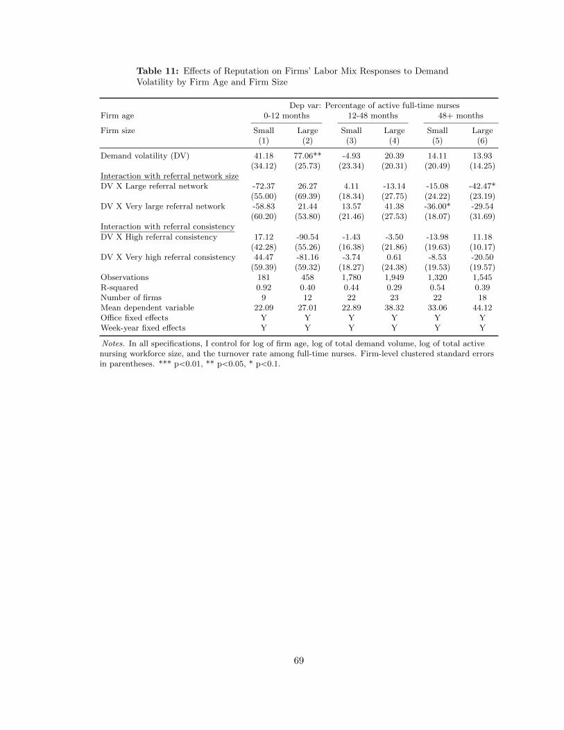
Table 11: Effects of Reputation on Firms’ Labor Mix Responses to DemandVolatility by Firm Age and Firm Size
Dep var: Percentage of active full-time nursesFirm age 0-12 months 12-48 months 48+ months
Firm size Small Large Small Large Small Large(1) (2) (3) (4) (5) (6)
Demand volatility (DV) 41.18 77.06** -4.93 20.39 14.11 13.93(34.12) (25.73) (23.34) (20.31) (20.49) (14.25)
Interaction with referral network sizeDV X Large referral network -72.37 26.27 4.11 -13.14 -15.08 -42.47*
(55.00) (69.39) (18.34) (27.75) (24.22) (23.19)DV X Very large referral network -58.83 21.44 13.57 41.38 -36.00* -29.54
(60.20) (53.80) (21.46) (27.53) (18.07) (31.69)Interaction with referral consistency
DV X High referral consistency 17.12 -90.54 -1.43 -3.50 -13.98 11.18(42.28) (55.26) (16.38) (21.86) (19.63) (10.17)
DV X Very high referral consistency 44.47 -81.16 -3.74 0.61 -8.53 -20.50(59.39) (59.32) (18.27) (24.38) (19.53) (19.57)
Observations 181 458 1,780 1,949 1,320 1,545R-squared 0.92 0.40 0.44 0.29 0.54 0.39Number of firms 9 12 22 23 22 18Mean dependent variable 22.09 27.01 22.89 38.32 33.06 44.12Office fixed effects Y Y Y Y Y YWeek-year fixed effects Y Y Y Y Y Y
Notes. In all specifications, I control for log of firm age, log of total demand volume, log of total activenursing workforce size, and the turnover rate among full-time nurses. Firm-level clustered standard errorsin parentheses. *** pă0.01, ** pă0.05, * pă0.1.
69
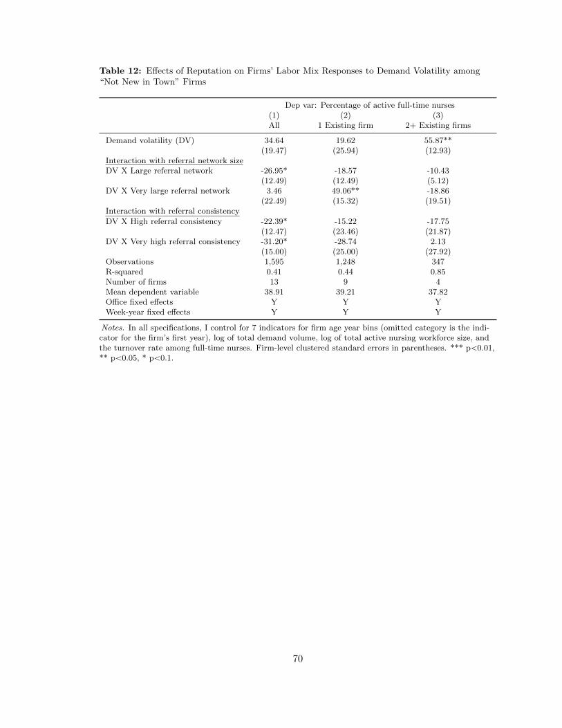
Table 12: Effects of Reputation on Firms’ Labor Mix Responses to Demand Volatility among“Not New in Town” Firms
Dep var: Percentage of active full-time nurses(1) (2) (3)All 1 Existing firm 2+ Existing firms
Demand volatility (DV) 34.64 19.62 55.87**(19.47) (25.94) (12.93)
Interaction with referral network sizeDV X Large referral network -26.95* -18.57 -10.43
(12.49) (12.49) (5.12)DV X Very large referral network 3.46 49.06** -18.86
(22.49) (15.32) (19.51)Interaction with referral consistency
DV X High referral consistency -22.39* -15.22 -17.75(12.47) (23.46) (21.87)
DV X Very high referral consistency -31.20* -28.74 2.13(15.00) (25.00) (27.92)
Observations 1,595 1,248 347R-squared 0.41 0.44 0.85Number of firms 13 9 4Mean dependent variable 38.91 39.21 37.82Office fixed effects Y Y YWeek-year fixed effects Y Y Y
Notes. In all specifications, I control for 7 indicators for firm age year bins (omitted category is the indi-cator for the firm’s first year), log of total demand volume, log of total active nursing workforce size, andthe turnover rate among full-time nurses. Firm-level clustered standard errors in parentheses. *** pă0.01,** pă0.05, * pă0.1.
70

Table
13:
Rob
ust
nes
sC
hec
kw
ith
Mark
etC
on
dit
ion
Contr
ols
:E
ffec
tsof
Rep
uta
tion
on
Fir
ms’
Lab
or
Mix
Res
pon
ses
toD
eman
dV
olat
ilit
y
Dep
var:
Per
centa
ge
of
act
ive
full-t
ime
nu
rses
(1)
(2)
(3)
(4)
(5)
(6)
(7)
(8)
(9)
Dem
an
dvola
tility
(DV
)25.0
3*
25.1
2*
24.4
9*
15.9
115.7
015.4
623.0
722.7
622.0
2(1
2.6
2)
(12.5
2)
(12.3
6)
(12.4
9)
(12.5
0)
(12.1
5)
(15.3
7)
(15.3
8)
(15.0
7)
Inte
ract
ion
wit
hre
ferr
al
net
work
size
DV
XL
arg
ere
ferr
al
net
work
-24.3
7*
-23.8
3*
-22.5
1*
-24.6
8*
-24.1
9*
-22.8
7*
(12.5
2)
(12.5
4)
(12.7
1)
(12.7
3)
(12.7
8)
(12.9
8)
DV
XV
ery
larg
ere
ferr
al
net
work
-4.9
9-4
.92
-3.8
3-5
.48
-5.5
9-4
.54
(16.2
3)
(16.3
0)
(16.1
1)
(15.1
5)
(15.2
7)
(15.1
6)
Inte
ract
ion
wit
hre
ferr
al
con
sist
ency
DV
XH
igh
refe
rral
con
sist
ency
2.2
63.1
13.3
43.1
13.9
54.0
0(1
1.8
7)
(11.9
7)
(11.8
5)
(11.1
0)
(11.2
0)
(11.1
6)
DV
XV
ery
hig
hre
ferr
al
con
sist
ency
5.4
06.3
36.7
95.7
66.6
87.0
7(1
4.6
0)
(14.6
0)
(14.4
5)
(13.3
8)
(13.3
8)
(13.3
0)
Ob
serv
ati
on
s3,3
44
3,3
44
3,3
44
3,3
44
3,3
44
3,3
44
3,3
44
3,3
44
3,3
44
R-s
qu
are
d0.4
00.4
00.4
10.4
00.4
00.4
00.4
00.4
00.4
1M
ean
dep
end
ent
vari
ab
le33.0
633.0
633.0
633.0
633.0
633.0
633.0
633.0
633.0
6M
ark
etle
vel
dem
an
dvola
tility
YY
YY
YY
Hom
eh
ealt
hm
ark
etco
mp
etit
ion
YY
YO
ffice
fixed
effec
tsY
YY
YY
YY
YY
Wee
k-y
ear
fixed
effec
tsY
YY
YY
YY
YY
Notes.
Inall
spec
ifica
tions,
Ico
ntr
ol
for
7in
dic
ato
rsfo
rfirm
age
yea
rbin
s(o
mit
ted
cate
gory
isth
ein
dic
ato
rfo
rth
efirm
’sfirs
tyea
r),
log
of
tota
lde-
mand
volu
me,
log
of
tota
lact
ive
nurs
ing
work
forc
esi
ze,
and
the
turn
over
rate
am
ong
full-t
ime
nurs
es.
Iuse
the
sub-s
am
ple
per
iod
of
2013–2014
due
tolim
ited
data
availabilit
yon
the
mark
et-l
evel
contr
ols
.F
irm
-lev
elcl
ust
ered
standard
erro
rsin
pare
nth
eses
.***
pă
0.0
1,
**
pă
0.0
5,
*p
ă0.1
.
71

2.9. Appendix: Proofs
Proof. (Proposition 1) I examine the effect of σ on p˚ relative to the effect of σ on s˚. Bytotal differentiation of (2.12), I obtain
Bs˚tBσ
“
12c2ppp
˚t q?Rt
c2sps˚t q `
12c2ppp
˚t q
(2.21)
Bp˚tBσ
“a
Rt ´Bs˚tBσ
“c2sps
˚t q?Rt
c2sps˚t q `
12c2ppp
˚t q. (2.22)
Thus, when demand volatility σ increases, p˚ increases faster than s˚ if
Bp˚tBσBs˚tBσ
“c2sps
˚t q
12c2ppp
˚t qą 1 or 2c2sps
˚t q ą c2ppp
˚t q. (2.23)
(2.23) shows that the firm increases piece-rate labor more than salaried labor in responseto higher demand volatility unless the difference in the rates of increase in marginal costsof the two types of labor is very large. In this example, the rate of increase in the marginalcost of piece-rate labor has to be less than twice the rate of increase in the marginal costof salaried labor by the construction of the stochastic distribution of demand.
Proof. (Proposition 2) To simplify the analysis, I plug in (2.13) for the ratio on the right-hand side of (2.16) and obtain
M ”EpBRt`2{BRt`1q
EpBRt`2{Bst`1q“
1´ γ
γ
st`1
Rt`1ą 0. (2.24)
I plug in (2.24) when differentiating the equation (2.16).
Furthermore, I assume convex labor cost functions as follows,
cspstq “1
2ax2 and cppxq “
1
2bx2, (2.25)
where a ă b is assumed since temporary labor is less productive or lacks firm-specific skills,requiring more training.
The derivative of the LHS of (2.16) with respect to σ is
Ed
dσπ1tpstq “ Eπ2t pstq
dstdσ
. (2.26)
The derivative of the first term before the brackets on the RHS of (2.16) with respect to σis
Ed
dσR1t`1pstq “ ER2t`1pstq
ˆ
dstdσ`dQtdσ
˙
“ ER2t`1pstqdstdσ
(2.27)
72

since EdQt
dσ “ 0. Let B denote the terms in the brackets on the RHS of (2.16):
B “ Eˆ
Bπt`1
Bst`1
˙
EpBRt`2{BRt`1q
EpBRt`2{Bst`1q´ E
Bπt`1
BRt`1. (2.28)
After plugging (2.24) into (2.28), I obtain the derivative of B with respect to σ:
dB
dσ“ ps1t`1pσq `R
1t`1pσqqrπ
2t`1pst`1qM ´ π2t`1pRt`1qs
` EBπt`1
Bst`1
ˆ
R1t`1pσq
Rt`1M `
1´ γ
γ
s1t`1pσq
Rt`1
˙
.(2.29)
It follows from (2.13) that
R1t`1pσq “γ
stRt`1s
1tpσq. (2.30)
Using the results from (2.26), (2.27), (2.29), (2.30), total differentiation of (2.16) is givenby
Eπ2t pstqdstdσ
“ β
„
ER2t`1pstq
ˆ
dstdσ
˙
B ` EBRt`1
Bst
dB
dσ
(2.31)
which can be rewritten, using (2.29), as
s1tpσq ”dstdσ
“
βs1t`1pσq
„
ER1t`1pstqK `1´γγ
Eπ1t`1pst`1q
Rt`1
Eπ2t pstq ´ β„
ER2t`1pstq `γstRt`1ER1t`1pstqK `
γstEπ1t`1pst`1qM
(2.32)
whereK “ Eπ2t`1pst`1qM ´ π2t`1pRt`1q. (2.33)
I show that the sign of s1tpσq depends on Rt. Since the expression is rather unwieldy, Iswitch now to more heuristic arguments to determine the sign. First, I assume that s1tpσqand s1t`1pσq have the same sign. Second, in the numerator, I know from (2.17) and (2.18)that ER1t`1pstq ą 0 and Eπ1t`1pst`1q ă 0, respectively. Moreover, p1 ´ γq{γ, Rt`1 ą 0. Todetermine the sign of K, note that
Eπ2t`1pst`1q “ ´c2spst`1q ´
1
2c2ppµRt`1 ` σ
a
Rt`1 ´ st`1q ă 0, (2.34)
73
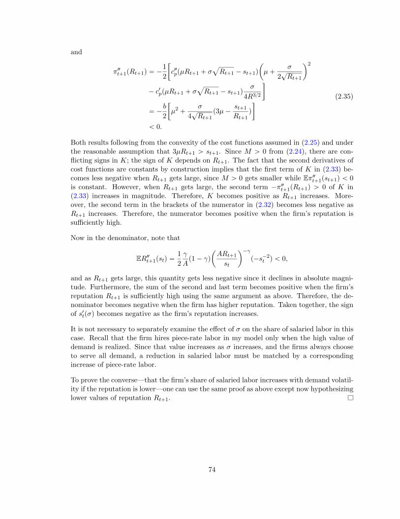
and
π2t`1pRt`1q “ ´1
2
„
c2ppµRt`1 ` σa
Rt`1 ´ st`1q
ˆ
µ`σ
2?Rt`1
˙2
´ c1ppµRt`1 ` σa
Rt`1 ´ st`1qσ
4R3{2
“ ´b
2
„
µ2 `σ
4?Rt`1
p3µ´st`1
Rt`1q
ă 0.
(2.35)
Both results following from the convexity of the cost functions assumed in (2.25) and underthe reasonable assumption that 3µRt`1 ą st`1. Since M ą 0 from (2.24), there are con-flicting signs in K; the sign of K depends on Rt`1. The fact that the second derivatives ofcost functions are constants by construction implies that the first term of K in (2.33) be-comes less negative when Rt`1 gets large, since M ą 0 gets smaller while Eπ2t`1pst`1q ă 0is constant. However, when Rt`1 gets large, the second term ´π2t`1pRt`1q ą 0 of K in(2.33) increases in magnitude. Therefore, K becomes positive as Rt`1 increases. More-over, the second term in the brackets of the numerator in (2.32) becomes less negative asRt`1 increases. Therefore, the numerator becomes positive when the firm’s reputation issufficiently high.
Now in the denominator, note that
ER2t`1pstq “1
2
γ
Ap1´ γq
ˆ
ARt`1
st
˙´γ
p´s´2t q ă 0,
and as Rt`1 gets large, this quantity gets less negative since it declines in absolute magni-tude. Furthermore, the sum of the second and last term becomes positive when the firm’sreputation Rt`1 is sufficiently high using the same argument as above. Therefore, the de-nominator becomes negative when the firm has higher reputation. Taken together, the signof s1tpσq becomes negative as the firm’s reputation increases.
It is not necessary to separately examine the effect of σ on the share of salaried labor in thiscase. Recall that the firm hires piece-rate labor in my model only when the high value ofdemand is realized. Since that value increases as σ increases, and the firms always chooseto serve all demand, a reduction in salaried labor must be matched by a correspondingincrease of piece-rate labor.
To prove the converse—that the firm’s share of salaried labor increases with demand volatil-ity if the reputation is lower—one can use the same proof as above except now hypothesizinglower values of reputation Rt`1.
74
CHAPTER 3 : The Effect of Workforce Assignment on Performance
3.1. Introduction
Workforce allocation and scheduling are routinely designed to achieve multiple organiza-
tional goals, with efficiency typically viewed as the leading objective.1 Efficient workforce
assignment entails the matching of task and talent (Garicano and Santos, 2004), manage-
ment of planned and unplanned absences (Ehrenberg, 1970; Allen, 1983), exigency and
geographical optimization, and responsiveness to demand shocks (Hamermesh and Pfann,
1996). Beyond efficiency, workforce allocation goals may include rewarding seniority, pro-
moting workforce equity, and enabling effective learning and synergy (Mas and Moretti,
2009). These goals potentially compromise short-term efficiency but at the same time raise
employee satisfaction and reduce costly turnover. Another set of objectives is linked with
the use of workforce assignment to achieve higher quality. While often in conflict with cost
minimization goals, higher quality may be rewarded directly through higher willingness to
pay and indirectly through increased reputation.
Hospitals and health care systems implement strategies to improve the quality of care for all
patients through focusing on patient safety, reducing medical errors, establishing evidence-
based guidelines, and lowering the rate of unnecessary and preventable intervention (Kozak
et al., 2001; Makary and Daniel, 2016). In fact, ensuring continuity of care within and
across care settings is identified as a pillar of quality improvement (Richardson et al., 2001).2
Continuity of care across settings involves, by definition, a multi-professional pathway that
emphasizes the need for care coordination. On the other hand, continuity of care within
a setting is achieved by workforce allocation, and in particular a continuous relationship
between a patient and a single health care professional who is the sole source of care and
information for the patient.
1This chapter is coauthored by Guy David.2Continuity of care has also been shown to reduce utilization and costs of care (Raddish et al., 1999),
such as by reducing the number of emergency department visits and shortening the length of hospital stays(Wasson et al., 1984).
75

However, the achievement of continuity of care requires costly deployment of resources. En-
suring smooth transitions in care and effective transmission of information between providers
likely imposes massive constraints that interfere with the goal of optimizing scheduling to
minimize workforce turnover and contractual disruptions. Thus, efficient workforce assign-
ment may lead to reductions in quality of care through compromised care continuity. Using
a novel data set from a large multi-state freestanding home health agency, this chapter
quantifies the effect of within-setting care discontinuity caused by workforce assignment on
hospital readmissions, a common quality of care marker.
Spending due to unplanned hospital readmissions was estimated at $17.4-$25 billion annu-
ally, which would translate to 16-22% of the total Medicare spending on inpatient hospital
services (Pricewaterhouse Coopers’ Health Research Institute, 2008; Jencks et al., 2009).
The national all-cause potentially preventable readmission rates for this population was
11% in 2014 (MedPAC, 2016b). Starting in October 2012, the Center for Medicare and
Medicaid Services (CMS) lowered its payment to hospitals with excess readmissions over
the national average by up to 3%.3 Facing financial penalties, hospitals use management
strategies and modifications to their organizational structure to prevent hospital readmis-
sions. For example, hospitals vertically integrated with post-acute care providers such as
home health agencies (HHAs) to improve post-discharge care coordination, as increased
reliance on home health has been shown to be associated with a reduction in hospital read-
missions (Polsky et al., 2014).4 Moreover, hospitals rely on post-acute care entities to reduce
avoidable readmissions (Naylor et al., 2012). Once patients are discharged from hospitals,
post-acute care providers monitor and treat still frail patients over an extended period of
time.5 Thus, post-acute care providers can impact the frequency of hospital readmissions
3The amount of reduction in payment was up to 1 percent in FY 2013, the first year of the HRRP, andup to 2 percent in FY 2014.
4Naylor et al. (1999) discuss hospitals that instituted programs to provide patient education beforedischarge, increased patient follow-up, and expanded the use of health information technology to trackreadmissions and integrate care across settings; Kim et al. (2015) show that admitting ER patients to theIntensive Care Units could substantially reduce hospital readmissions, and therefore suggest implementingadmission criteria based on objective measures of patient risk as well as physicians’ discretionary informationas a promising way to decrease hospital readmissions.
5In the case of home health care, the default length of an episode is 60 days for Medicare patients.
76
by implementing workforce assignment strategies that promote care continuity.
We focus on home health care as it is an important and rapidly growing segment of the
health care delivery system. Over the past decade, payment for home health services more
than doubled (MedPAC, 2016a). This rapid growth may be attributed to its appeal to
patients who prefer to recover at home, providers who prefer to shorten hospitalization
lengths, and insurers who benefit from cheaper care at home than care in brick-and-mortar
institutions. Home health care is recognized as a partial substitute for institutional long-
term care (Guo et al., 2015). The importance of home health care has also increased with
the rise of enhanced care coordination and shared savings models such as Accountable Care
Organizations or Bundled Payments for Care Improvement (Sood et al., 2011).
Studying the intricacies of home health care provision and its impact on hospital read-
missions is timely and important. Before the ACA, there was no competitive pressure for
HHAs and no financial incentives to reduce readmissions, with three in ten post-acute home
health stays resulting in a hospital readmission among Medicare patients (MedPAC, 2014).6
However, with readmission penalties and the emphasis on population health management,
home health has become a way to allow for continuity of care outside of the hospital and
effectively manage the patient health to prevent unnecessary readmissions. Freestanding
agencies often view the ability to mitigate hospital readmission as a key competitive differ-
entiator in contracting with hospitals (Worth, 2014). Therefore, it is important to uncover
potential mechanisms that lead to better care continuity and patient outcomes.
In this chapter, we use novel data containing over 43,000 home health patient episodes and
spanning 89 autonomously run home health offices in 16 states. The data provide detailed
information, which includes visit logs for all Medicare patients, work logs and human re-
sources data for all home health providers, as well as all patient demographic and health
risks collected as part of the Outcome and Assessment Information Set (OASIS) required by
6This figure could also be attributed to the fact that patients being discharged to home health care tendto be sicker and at a higher risk of hospital readmissions that those being discharged to home.
77
the CMS. In addition, our data are linked with individual patients’ hospital readmissions.
We measure care discontinuity by handoffs between skilled nurses over a patient’s episode
of care, which are immediately affected by offices’ workforce allocation decisions.7 We esti-
mate a plausibly causal effect of provider handoffs on hospital readmissions using day-to-day
human resources data on providers’ absence, assignment to an alternative office, and job
termination to instrument for handoffs. Unplanned employee absences in the US health care
and social assistance sector consumed 1.9% of all scheduled work hours in 2016 (Bureau
of Labor Statistics, 2017). To uncover the mechanisms underlying the effect of handoffs,
we also examine whether the probability of readmission is affected by the frequency and
sequencing of handoffs.
Estimating the effect of handoffs in home health care on the probability of readmissions
raises endogeneity concerns. While we observe a great deal of patient characteristics as
well as labor supply conditions, the data do not provide us with the actual care plan for
each patient’s episode of care. The care plan is plausibly linked to unobserved patient
severity and hence to the risk of hospital readmissions. As we discuss in the chapter, it
is challenging to determine the sign of the omitted variable bias caused by unobserved
patient characteristics. To address this endogeneity problem, we use detailed provider-
day level data on nurses’ availability to instrument for both handoffs and the probability
of receiving a visit. The instrument exploits the fact that skilled nurses’ absence affects
rehospitalization only through its effect on care discontinuity either through missed visits
or handoffs. In addition, and as explained in greater detail in our methods section, we
control for the dynamic changes in patients’ health status during a home health episode by
limiting the variation in our data to reflect the number of days since the last nurse visit;
the mean interval of days between two consecutive nurse visits; the passage of time from
the beginning of the episode; the relationship stock with various nurses during the episode;
as well as supply and demand characteristics at the nurse and office level. Together with
the patient’s initial health assessment, these controls help mitigating potential confounding
7Skilled nurses refer to registered nurses (RNs) or licensed practical nurses (LPNs).
78

effects.
Using the cross-sectional variation, we find that patients experiencing nurse handoffs are
19% more likely to be readmitted to a hospital. This estimate more than doubles in magni-
tude when using the instrumental variables approach. Our results are robust to controlling
for days since last visit as well as a rich set of patients’ health risk, demographic, and co-
morbidity factors, office fixed effects, time fixed effects, and home health day fixed effects.
Controlling for home health day fixed effects is especially important because the probabili-
ties of hospital readmissions and handoffs rapidly decline over the course of a home health
episode.
To explore potential mechanisms underlying this effect, we analyze finer partitions of hand-
offs by frequency and sequencing. We find the effect of first handoffs to have the strongest
effect on increasing the likelihood of hospital readmissions, with the second and third hand-
offs having effects that are smaller in magnitude. The effect of having four or more handoffs
is no longer statistically significant. Our finding that initial handoffs are more impactful
than subsequent ones, controlling for elements of the patient episode dynamics, suggests
that to effectively reducing hospital readmissions, it is important to ensure provider conti-
nuity throughout the entire episode of care.
A number of potential mechanisms may account for the effect of provider handoffs on hos-
pital readmissions. First, information transmission between providers involved in a handoff
may be incomplete and lead to potentially inappropriate care (Riesenberg et al., 2009).
Second, holding the number of visits constant, handoffs lower the time spent with each in-
dividual provider, and hence depreciates the relationship stock built between providers and
patients, which has been shown to improve patient outcomes (Saultz and Lochner, 2005).
Third, repeated visits enhance the development of patient-specific knowledge, which has
limited applicability to other patients. Therefore, patients experiencing a handoff lose ac-
cess to providers most familiar with their case. For example, previous literature emphasizes
the development of firm- or patient-specific skills among cardiac surgeons and radiologists,
79
which are associated with a reduction in patient mortality rates (Huckman and Pisano,
2006). The three channels above serve as theoretical underpinning for our findings of a
positive link between provider handoffs and hospital readmissions.
In summary, this chapter provides the first set of results linking care discontinuity in a
post-acute care setting to increased risk of hospital readmissions. To date, most of the
literature on care continuity has focused on transitions of care across settings, especially
on care transitions from hospitals to post-acute care facilities (Naylor et al., 1999). Work
on continuity of care within a setting has focused almost exclusively on patient handoffs
in shift-based environments, which are shown to be associated with low quality of care
marked by slowdown in service delivery, medical and surgical errors, malpractice cases with
communication problems, and (potentially preventable) adverse patient outcomes (Laine
et al., 1993; Petersen et al., 1994; Riesenberg et al., 2009). However, the external validity
of results in a shift-based environment may be weak when considering non-shift based
environments, such as home health. Shift-based handoffs are inevitable due to a trade-off
between the length of a shift and the number of handoffs. When physician or nurse shifts are
lengthened, a patient is more likely to see the same provider during the course of treatment.
At the same time, a longer shift would increase provider fatigue and the risk of making
mistakes, especially, towards the end of long shifts (Brachet et al., 2012). In contrast, in
home health care, handoffs are largely avoidable through coordinated scheduling given that
providers typically visit patients with several days in between. In our data, 38% of patients
are seen consistently by a single nurse throughout their episode of care. Hence, zero handoffs
are frequent in a non-shift based environment. At the same time, prioritizing continuity of
care may be costly in that it may come at the expense of flexibility in scheduling, employee
satisfaction, and ultimately retention.
Quantifying the effect of discontinuous home health care has important implications for the
use of workforce assignment in improving quality of care, and provides a currency to assess
the importance of prioritizing care continuity over other goals typically achieved through
80
schedule architecture. Previous literature has focused almost exclusively on shift-based
provider handoffs in large healthcare facilities. Moreover, the literature has focused mostly
on nurse staffing levels rather than assignment structure among the workforce strategies
used by health care delivery organizations (Aiken et al., 2002; Bae et al., 2010; Needleman
et al., 2011; Cook et al., 2012; Lin, 2014; Lu and Lu, 2016; Hockenberry and Becker, 2016).
The outline of the article is as follows. In Section 3.2, we describe the data and present
our measures of care discontinuity. In Section 3.3, we discuss our identification strategy. In
Section 3.4, we discuss our baseline empirical results as well as our IV estimation results. In
Section 3.4.3, we explore the sequencing of handoffs in explaining the relationships between
handoffs and the rehospitalization outcome. Section 3.5 concludes the chapter.
3.2. Data
3.2.1. Data and Summary Statistics
This chapter uses a novel and rich data set of home health visits, patient health status
assessment, and provider work logs as well as indicators for patient hospital readmissions.
We obtained data on all home health stays for Medicare patients from a large for-profit
freestanding home health company, which provides home health care services in 89 offices
in 16 states.89 Since each office autonomously decides scheduling and staffing and is run as
a profit center, we can regard each office as a separate hiring and contracting unit in our
empirical analysis. This large set of independently run offices alleviates some concern about
the generalizability of our results to other HHAs even if they all belong to one company.10
8These offices are located in 16 states: Arizona, Colorado, Connecticut, Delaware, Florida, Hawaii,Massachusetts, Maryland, North Carolina, New Jersey, New Mexico, Oklahoma, Pennsylvania, Rhode Island,Virginia, Vermont.
9David et al. (2013) show that in vertically integrated HHAs owned by hospitals, post-acute care patientsare admitted to HHAs in earlier stages of recovery without a significant difference in readmission rates.
10During 2013, compared to a national sample of freestanding agencies, home health offices in our sampletend to be larger, have a lower share of visits provided for skilled nursing and instead have a higher shareof visits provided for therapy, and have a lower share of episodes provided to dual-eligible Medicare orMedicaid beneficiaries, which seem to be more common characteristics of proprietary agencies (Cabin et al.,2014; MedPAC, 2016a). However, home health offices in our data provide a similar total number of visitsper episode and serve a similar age group on average.
81
Our sample period covers 44 months between January 2012 and August 2015, for which we
have full patient, worker, and office data.
Our main outcome is hospital readmission, which is an important marker of quality and
can potentially lead to financial penalties for hospitals. Rehospitalizations among patients
receiving home health is common. Our analysis focuses on Medicare patients, who comprise
a majority of home health patients and have a high probability of hospital readmissions.11
Furthermore, our analysis focuses on care discontinuity for skilled nursing because most
visits are for skilled nursing care and it provides most medically relevant service that could
potentially determine the likelihood of hospitalization (Russell et al., 2011).12
Our patient data are provided at the patient visit level as well as the patient episode-
admission level.13 To construct our patient-day level data, we merge the patient episode
level data with the visit level data. Home health episodes can end by either a discharge or
a hospitalization. The exact dates of these end points for each episode are obtained from
the home health admission level OASIS data. These data also provide a rich set of health
risk factors.
We also obtained human resources data containing work logs for all providers’ visits. We
merge the patient-day level data with provider-day level work log data to identify hand-
offs and link them with hospital readmissions. Separately, we also use the provider-day
level work logs to construct instruments of providers’ inactivity statuses, as described in
Section 3.3.4.
Finally, we construct office-day level data spanning all 89 offices. This data set tracks
ongoing episodes and all nurses in each office providing services on each day. This is then
11In the data, on average, 69% of home health episodes in each month are paid for by Medicare (includingall Medicare FFS, private Medicare Advantage, and Medicare Part B) either as a primary or secondary payeracross 93 offices and months during the sample period. Nationally, Medicare patients had 29% readmissionrates among post-hospital home health stays (MedPAC, 2014).
12In addition to nurses, there are typically additional providers who visit patients during a home healthepisode. Those include home health aides, physical therapists, speech-language pathologists, occupationaltherapists, and medical social services workers.
13Medicare FFS pays a prospective payment for each 60-day episode. For patients requiring more care,episodes may be extended by another 60 days during a given home health admission.
82
merged with the patient-day level data to provide office-level demand and supply conditions.
To construct our final patient-day level sample for analyses, we exclude patients who had
multiple subsequent home health episodes as these home health stays may have different pat-
terns of visit schedules and provider handoffs.14 Since our measure of care discontinuity—
handoffs—occur across visits, we exclude episodes consisting of a single visit. Finally, we
restrict to home health episodes with a prior hospitalization in the past 14 days.15 Our
final sample includes 43,740 unique home health episodes and 1,031,904 patient days under
home health.
Table 14 reports the summary statistics at different levels of aggregation: Panel A at the
office-day level; Panel B at the patient-episode level; and Panel C at the patient episode-
day level. In our sample, 16.6% of episodes involve a hospital readmission, and most of
the readmissions occur within 30 days of hospital discharge.16 The average home health
episode in our sample involved 6 nurse visits over a period of 33 days, with 87% of home
health episodes involving between 3 and 12 nurse visits.
Figure 6 presents the number of ongoing episodes and number of readmissions occurring
by home health day. It suggests that both the probabilities of being under home health
care and readmission decline with home health days. Thus, we control for day of home
health fixed effects as well as the number of visits and days since last visit to examine
the effect of discontinuous care on the probability of rehospitalization across patients with
identical number of visits, spacing of visits, and episode length. We discuss this further in
Section 3.3.1.
14More precisely, enrolling patients into subsequent episodes has been shown to exhibit a degree of strategicbehavior. For example, after the introduction of the home health prospective payment system in 2000,agencies increased the number of episodes per patient (Kim and Norton, 2015).
15Home health admissions preceded by a hospital stay account for 35.5% of all Medicare home healthadmissions in our sample.
16Another outcome reported in the OASIS survey is death at home. We do not use it as an outcomebecause it is rare. Out of more than one million patient-days, death occurs at a rate of 0.18%.
83

3.2.2. Measuring Care Discontinuity: Provider Handoffs
We focus on the notion of provider handoffs to measure care discontinuity. Many studies
on care discontinuity focused on shift-based settings in which there is a salient trade-off
between the length of shifts and quality of care (Laine et al., 1993; Petersen et al., 1994;
Riesenberg et al., 2009; Brachet et al., 2012). By making the shifts longer, you can provide
more continuous care but this comes at the expense of providers’ fatigue towards the end of
the shifts. In contrast, in home health care settings, handoffs can plausibly be eliminated
since 24/7 coverage is rare and visits are typically provided with several days in between. In
our sample, the average number of days between visits is 5. Thus, continuous home health
care can be naturally conceptualized as seeing the same provider repeatedly, and discontin-
uous care as a break in it—a provider handoff. Handoffs can also capture a disruption in
important aspects of care continuity—uninterrupted service delivery and trusting relation-
ship between service provider and client or caregiver—emphasized by the key stakeholders
in the home health industry (Woodward et al., 2004).
For the estimation, we define a “handoff state” as a series of days, beginning on the day
a visit by a different skilled nurse occurs and ending on one day before the day that the
same skilled nurse visits again (i.e. when continuity of care is restored). Put differently, for
each patient i and day t, an indicator of having a nurse handoff equals 1 if i’s last nurse is
different from the nurse who cared for i in the preceding visit; and 0 otherwise.17 Under
this definition of handoffs, only 38% of patient episodes experience no handoff during the
episode of care, with the remaining 62% of patient episodes having at least on handoff.
Figure 7 tracks additional variants of handoffs across the home health episode’s length.
Figure 7 links home health day with the fraction of patient episodes with at least one, two,
three or four handoffs. By the 10th home health day, the fraction of episodes with at last
17Under this definition of handoffs, a patient could be in a handoff state even on days she has no nursevisit if those days follow a visit during which an actual handoff occurred. We choose this definition becausewe view that a patient is “at risk” of being readmitted to a hospital after a handoff occurs. Our results arerobust to restricting the sample only to visit days (results are available upon request).
84
one handoff is 54%, 18% with at least two handoffs, 4% with at least three handoffs, and
1% with at least four handoffs. In comparison, by the 30th home health day, the fraction of
episodes with at least one handoff is 64%, 39% with at least two handoffs, 21% with at least
three handoffs, and 11% with at least four handoffs. Similarly, Figure 8 shows the fraction
of patient-days with nurse handoffs conditional on having a nurse visit. Again, handoffs are
substantially more likely to occur early in the home health episode and then sharply decline
with more home health days.
3.3. Empirical Strategy
3.3.1. Baseline Specification
We estimate linear probability models with the following specification:
Readmitikt “ α` βHikt ` γVikt ` δ1Xikt ` δ2Pik ` δ3Wkt ` δ4Dt ` θk ` εikt (3.1)
where Readmitikt is an indicator variable for whether patient i served by office k is readmit-
ted to a hospital on day t; Hikt is an indicator variable for handoffs described in Section 3.2.2;
Vikt is an indicator variable for having a nurse visit; Xikt is a vector of patient-office-day
level variables; Pik is a vector of patient-office-level variables; Wkt is a vector of office-day
level variables; Dt is a day-level variables; θk is office fixed effects.
Whether a patient is readmitted to a hospital may depend on the progression of her severity
over the course of home health care, making it important to control for dynamic changes in
the patient’s daily health status. Beyond an initial assessment in the first visit, home health
agencies do not systematically measure and collect data on the patient’s health status in
subsequent visits. Therefore, we cannot directly control for the dynamic changes in patients’
health. However, we use a number of dynamic proxies of patients’ real-time health status.
First, we control for whether a patient has a nurse visit on a given day, Vikt, as a sicker
patient is more likely to have a nurse visit. Second, we control for the number of days since
last visit by a nurse in the vector Xikt together with the patient-level mean interval of days
85

between consecutive nurse visits in the vector Pik. The variation in the number of days
since last nurse visit holding constant the expected frequency of visits during the episode
could capture dynamic shifts in the patient’s severity since a nurse’s additional visit only
after a short period of time may suggest that the patient has gotten sicker on that day.
Third, for similar reasons, we include in the vector Xikt of patient-office-day level variables
the number of days since last visit by any provider since the greater the gap between any
home health visits, the more likely a patient is to have a readmission controlling for the
average frequency of nurse visits. Fourth, we control for the cumulative number of nurse
visits provided to control for the effect of dynamic care intensity.18
In the vector Pik of patient level variables, we also include the following three groups of
variables to adjust for underlying health risks of patients. First, a set of indicator variables
associated with high risk of hospitalization, including history of 2 or more falls in the past
12 months, 2 or more hospitalizations in the past 6 months, a decline in mental, emotional,
or behavioral status in the past 3 months, currently taking 5 or more medications, and
others. Second, a set of indicator variables for patient demographics: age dummies for each
age 66-94 and age 95 or higher (reference group is age 65), gender, race, insurance type,
an indicator for having no informal care assistance available, and an indicator for living
alone.19 Third, a set of indicator variables for comorbidity factors, including indicators
for 17 Charlson comorbidity index factors, indicators for overall health status, indicators
for high-risk factors including alcohol dependency, drug dependency, smoking, obesity, and
indicators for conditions prior to hospital stay within past 14 days including disruptive
or socially inappropriate behavior, impaired decision making, indwelling or suprapublic
18Additional potentially relevant variables to include in the vector Xikt are the cumulative number ofunique nurses the patient has seen by home health day t and the number of times each nurse has seen thepatient. These variables capture an aspect of care disruption that is potentially more meaningful for patientsexperiencing a large number of handoffs. For example, a patient experiencing six handoffs may be caredfor by six different nurses, or may experience multiple handoffs between the same two nurses. Our resultsare robust and even stronger when controlling for these two additional variables (these results are availableupon request).
19Insurance types include Medicare Advantage (MA) plans with a visit-based reimbursement, MA planswith an episode-based reimbursement, and dual eligible with Medicaid enrollment (reference group is Medi-care FFS).
86
catheter, intractable pain, serious memory loss and/or urinary incontinence.20
In the vector Wkt of office-day level variables, we include the number of ongoing episodes
and the number of skilled nurses working in the office-day to control for the time-variant
caseload and labor supply conditions in each office.
The vector Dt includes indicators for each home health day, indicators for each day of
week, and indicators for each month-year. The home health day fixed effects absorb any
unobserved fixed characteristics of home health care depending on the timing within an
episode, as illustrated in Figures 6, 7, and 8. We also control for month-year pairs as
well as day of week indicators to control for any time-specific component of the variation
in the likelihood of readmission such as lower probability of readmission in months with
major holidays or weekends. The office fixed effects θk absorb time-invariant office-specific
or geographic differences in hospital readmissions, for example, through different hospital
policies or state regulations concerning patient readmissions, such as states with Certificate-
of-Need (CON) laws imposing home health entry restriction (Polsky et al., 2014). Our
estimates of the effects of handoffs would be based on the difference in the readmission
rates between patients who experience a nurse handoff and those who do not on the same
home health day, same month-year, day of week as well as in the same office after controlling
for other observed characteristics discussed above.
3.3.2. Identification Challenges
Indicator variables for experiencing a handoff and having a nurse visit are endogenous due to
the non-random provision of continuous care and nurse visits. To provide a plausibly causal
estimate of the effect of handoffs on hospital readmissions, we need to use an exogenous
measure of handoffs. To understand the identification strategy, rewrite the equation (3.1)
in a more general form where the readmission outcome Readmitikt is a function of hand-
offs Hikt; an indicator variable for having a nurse visit scheduled Vikt; other observable
20Indicators for overall health status include indicators for very bad (patient has serious progressive con-ditions that could lead to death within a year), bad (patient is likely to remain in fragile health) andtemporarily bad (temporary facing high health risks).
87
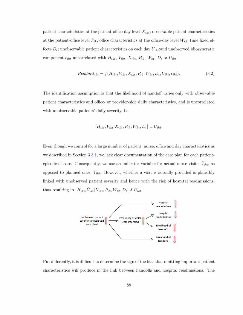
patient characteristics at the patient-office-day level Xikt; observable patient characteristics
at the patient-office level Pik; office characteristics at the office-day level Wkt; time fixed ef-
fects Dt; unobservable patient characteristics on each day Uikt;and unobserved idiosyncratic
component εikt uncorrelated with Hikt, Vikt, Xikt, Pik, Wkt, Dt or Uikt:
Readmitikt “ fpHikt, Vikt, Xikt, Pik,Wkt, Dt, Uikt, εiktq. (3.2)
The identification assumption is that the likelihood of handoff varies only with observable
patient characteristics and office- or provider-side daily characteristics, and is uncorrelated
with unobservable patients’ daily severity, i.e.
rHikt, Vikt|Xikt, Pik,Wkt, Dts K Uikt.
Even though we control for a large number of patient, nurse, office and day characteristics as
we described in Section 3.3.1, we lack clear documentation of the care plan for each patient-
episode of care. Consequently, we use an indicator variable for actual nurse visits, Vikt, as
opposed to planned ones, Vikt. However, whether a visit is actually provided is plausibly
linked with unobserved patient severity and hence with the risk of hospital readmissions,
thus resulting in rHikt, Vikt|Xikt, Pik,Wkt, Dts M Uikt.
Put differently, it is difficult to determine the sign of the bias that omitting important patient
characteristics will produce in the link between handoffs and hospital readmissions. The
88
reason is that unobserved severity is potentially linked with handoffs and readmissions both
directly and indirectly through care intensity. The direct link suggests that sicker patients
are both more likely to experience adverse outcomes leading to hospital readmissions and
less likely to experience handoffs since offices may try to provide more continuous care.
The indirect link is mediated by care intensity, that is, sicker patients will receive more
frequent visits during their episode of care. Higher care intensity lowers the risk of hospital
readmission but raises the likelihood of scheduling conflicts leading to handoffs. While
the direct link suggests fewer handoffs and higher likelihood of hospital readmissions, the
indirect link suggests the exact opposite.
3.3.3. Identification Strategies
As a first step to alleviate some of these concerns, we control for a rich set of patient-day
variables that serve as a proxy for dynamic changes in unobserved patient-day level severity,
as we explain in Section 3.3.1. These variables include the indicator for having a nurse visit
and the number of days since last visit by a nurse or any other provider holding constant
the mean frequency of nurse visits. To further address the potential threat of endogeneity,
we use detailed provider-day level data on breaks in nurses’ availability to instrument for
both handoffs and the probability of receiving a visit. The likelihood of having a nurse visit
is also endogenous as only the actual visits provided are observed and whether a patient
receives a nurse visit is correlated with unobservable daily severity level. The instrument
exploits the fact that skilled nurses’ absences for various periods of time and reasons affect
hospital readmission only through their effects on care discontinuity, that is either through
missed visits or handoffs.
Call the vector of nurse availability breaks measures Bikt. Suppose that assumptions hold
that (1) Bikt is strongly correlated with the endogenous variables Hikt and Vikt; (2) Bikt is
orthogonal to Uikt conditional on other vectors; and (3) the observable vectors are separable
from the last two unobserved vectors in fp¨q in equation (3.2). We can identify the causal
effect of provider handoffs on the likelihood of readmissions by estimating the system of
89
equation (3.2) and
Hikt “ gpBikt, Xikt, Pik,Wkt, Dt, Uikt, ηiktq (3.3)
Vikt “ hpBikt, Xikt, Pik,Wkt, Dt, Uikt, νiktq (3.4)
using the generalized method of moments, with the instrument moment condition
E„
!
Readmitikt ´ fpHikt, Vikt, Xikt, Pik,Wkt, Dtq
)
Bikt
“ 0 (3.5)
where ηikt and νikt in equations (3.3) and (3.4), respectively, are idiosyncratic error terms
for Hikt and Vikt uncorrelated with εikt and Uikt.
3.3.4. Breaks in Provider Availability
For the instrument set Bikt we use breaks in nurse availability on each day as a source of
exogenous variation in the likelihood of having a nurse handoff and having a nurse visit.
By merging the provider-day level data with the patient-day level data, we track whether
the nurse seen by patient i in the last visit is unavailable to serve i today. The last nurse
can be assigned to one of six mutually exclusive states in each office k on each day t: (1)
Active—visiting patients in i’s home office k; (2) Short absence—not providing visits in any
office for 1 to 6 consecutive days; (3) Medium absence—not providing visits in any office
for 7 to 14 consecutive days; (4) Long absence—not providing visits in any office for 15 to
90 consecutive days; (5) Assigned to other office—providing visits exclusively in a different
office; and (6) Attrition—not providing visits in any office for 91 or more consecutive days,
or having the employment contract terminated (due to either quit or layoff) according to
HR records.2122 The instrument vector Bikt includes the above absence indicator variables
(2)-(6) with “Active” the omitted category.
21We made a judicious choice of this definition of medium absence. We run a robustness check on ourmain results using an alternative definition of medium absence–not providing visits in any office for 6 to 20consecutive days–and find very similar results in Table 25 in Appendix 3.6.4.
22Since home health visits entail mobility as a nature of work, a provider is not constrained to work foronly one office and can visit patients in different offices.
90
For the validity of the instrument set Bikt, we require that CorrpBikt, rHikt, Vikts1q ‰ 0 and
Bikt K Uikt. For the former, it is intuitive that handoffs and missing a visit will be more likely
to occur on day t if the nurse who visited the patient in the last visit is unavailable to visit
her again on that day. Table 16 presents the distribution of the number of patient episode-
day observations as well as the likelihood of having a nurse handoff, a nurse visit, and a
hospital readmission for each availability category.23 In 65% of patient-day observations, the
last nurse who visited a patient is available for the same office. As expected, the probability
of handoff is lowest at 21% in this subsample compared to all other states corresponding
to providers’ unavailability. Handoffs occur in 60-70% of patient-day observations in which
the nurse who visited the patient in a preceding visit is either on medium or long absence.
Similarly, when the last nurse who visited the patient in a preceding visit is unavailable,
the patient is less likely to have a nurse visit. The probability of having a nurse visit is
approximately 10% or smaller when the last nurse is unavailable while the same probability
is 27% when the last nurse is around working at the same office. This comparison suggests
a strong correlation between nurses’ unavailability and handoffs. Consistent with this, we
find first-stage results to be quite strong, as shown later in Table 18.
As for the exclusion restriction, we rely on the notion that nurse inactivity is uncorrelated
with unobserved daily patient health conditions or any other unobserved nurse-day level
or office-day level characteristics. Such correlation would imply that absence by nurses
is linked with their patients’ likelihood of readmission. To assess these possibilities, we
discuss several ways in which the exclusion restriction condition could be violated and show
evidence alleviating those concerns.
First, a potential concern may be that nurses are more likely to become inactive when their
patients’ health changes. In particular, nurses with patients who are getting progressively
sicker may experience burnout and desire a day off. To assess such potential scenarios,
Figure 9 plots three key measures of patients’ severity by number of days prior to nurse
23We provide the same table using an alternative definition of absence categories in Table 24 in Ap-pendix 3.6.4.
91
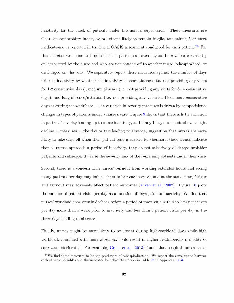
inactivity for the stock of patients under the nurse’s supervision. These measures are
Charlson comorbidity index, overall status likely to remain fragile, and taking 5 or more
medications, as reported in the initial OASIS assessment conducted for each patient.24 For
this exercise, we define each nurse’s set of patients on each day as those who are currently
or last visited by the nurse and who are not handed off to another nurse, rehospitalized, or
discharged on that day. We separately report these measures against the number of days
prior to inactivity by whether the inactivity is short absence (i.e. not providing any visits
for 1-2 consecutive days), medium absence (i.e. not providing any visits for 3-14 consecutive
days), and long absence/attrition (i.e. not providing any visits for 15 or more consecutive
days or exiting the workforce). The variation in severity measures is driven by compositional
changes in types of patients under a nurse’s care. Figure 9 shows that there is little variation
in patients’ severity leading up to nurse inactivity, and if anything, most plots show a slight
decline in measures in the day or two leading to absence, suggesting that nurses are more
likely to take days off when their patient base is stable. Furthermore, these trends indicate
that as nurses approach a period of inactivity, they do not selectively discharge healthier
patients and subsequently raise the severity mix of the remaining patients under their care.
Second, there is a concern than nurses’ burnout from working extended hours and seeing
many patients per day may induce them to become inactive, and at the same time, fatigue
and burnout may adversely affect patient outcomes (Aiken et al., 2002). Figure 10 plots
the number of patient visits per day as a function of days prior to inactivity. We find that
nurses’ workload consistently declines before a period of inactivity, with 6 to 7 patient visits
per day more than a week prior to inactivity and less than 3 patient visits per day in the
three days leading to absence.
Finally, nurses might be more likely to be absent during high-workload days while high
workload, combined with more absences, could result in higher readmissions if quality of
care was deteriorated. For example, Green et al. (2013) found that hospital nurses antic-
24We find these measures to be top predictors of rehospitalization. We report the correlations betweeneach of these variables and the indicator for rehospitalization in Table 23 in Appendix 3.6.3.
92

ipated high-workload days and strategically elected to take time off from work on those
days.25 However, we find no evidence of increases in office-level daily caseload, arrival of
new patients, or number of nurse visits immediately following the onset of absence. Fig-
ure 11 plots three office-day level measures: the total number of active patients (i.e. the
stock of ongoing episodes), the number of new (admitted) patients, and the total number
of nurse visits. These measures are plotted in the 10 days leading to a nurse absence and
the 10 days following the onset of a nurse absence. We find no evidence of an increase in
the office stock of episodes prior to absence.
Not surprisingly, absence reduces offices’ capacity for taking on new cases by about 30% in
the first two days following the onset of absence, although by the third day office are back
to pre-absence levels. Similarly, the total number of nurse visits falls following absence.
These findings strengthen the case for our instrument. Absence does not affect the stock of
episodes, but reduces the number of visits, hence fewer patients are visited due to absence
and those who are visited are likely to experience a handoff. Contrary to Green et al. (2013)
we find that nurses are inactive when office-level workload is stable, number of daily visits
is lower and fewer patients discharged from hospitals are seen for the first time by the office.
In summary, we expect nurse absence in a given day to be positively correlated with the
likelihood of handoffs and negatively correlated with the likelihood of visits, but presumably
uncorrelated with other factors influencing the likelihood of hospital readmissions. To the
extent that different lengths and types of absence provide an exogenous source of variation
in the likelihood of handoffs, changes in hospital readmissions should not be driven by nurse
absences.
25Workload in a hospital is likely unrelated to nurse staffing, that is, patients are not turned down byhospitals due to temporary fluctuation in nurse staffing. On the other hand, absence in home health is likelyto affect the agency’s ability to take on new patients and meet the care plan for existing patients. Thissuggests that the anticipated caseload may be systematically higher than the realized one.
93

3.4. Results on the Effects of Handoffs on the Likelihood of Rehospitalization
3.4.1. Baseline Results from the Cross-Sectional Estimation
Table 17 shows the baseline coefficient estimates on the handoff state indicator from our
cross-sectional analysis using four specifications representing different degrees of model sat-
uration, incrementally introducing additional patient level controls. In all columns, we
control for the indicator for having a nurse visit Vikt and variables in the patient-day level
vector Xikt, office-day level vector Wkt, day level time fixed effects vector Dt, and office
fixed effects θk, as described in Section 3.3.1. In Columns (2)-(4), we incrementally control
for the hospitalization risk, demographic, and comorbidity factors, respectively, whose de-
tailed description is provided above. In all these columns, the reference category is the case
of experiencing no handoffs. All reported standard errors allow for arbitrary correlation
among patient-day observations within the same office.
We find that within home health day, patients experiencing nurse handoffs are 0.17 per-
centage points or 24% more likely to have hospital readmissions in all specifications. When
restricting to 30-day rehospitalizations, the basis for hospital readmission penalties, the
effects of nurse handoffs are slightly lower at 21% increase (see Appendix 3.6.1). For ro-
bustness, we also estimate the effects using a fixed effect conditional logit estimation to
account for the binary nature of our dependent variable. These results are reported in
Appendix 3.6.2.
3.4.2. Results from the Instrumental Variables (IV) estimation
Table 18 reports IV estimation results from using the vector of instruments we discuss in
Section 3.3.4.26 We estimate a two-stage least square (2SLS) using a two-step efficient
generalized method of moments (GMM) estimator. Panels A and B report the first-stage
results for the indicator variables for having a nurse handoff and for a nurse visit, re-
26Table 25 in Appendix 3.6.4 shows the IV estimation results using an alternative definition of mediumabsence, as explained in Section 3.3.4.
94
spectively. We find the vector of instrumental variables to be a strong predictor of both
endogenous variables regardless of specification. The first-stage F-statistic values are large
(above 537 for handoffs and above 213 for visits ). In Panel A, not surprisingly, each one of
the instruments has a statistically significant positive association with handoffs, with longer
absence periods (medium, long and permanent absence) resulting in a greater likelihood of
handoffs. Similarly, in Panel B, each instrumental variable is negatively associated with the
probability of the patient receiving a nurse visit, although the difference in the magnitude
of the coefficient estimates is smaller. Panel C reports the second-stage results regress-
ing hospital readmission per-patient-episode-day on the predicted likelihood of handoff and
the predicted likelihood of a visit. We find handoffs to raise hospital readmissions, with a
statistically significantly coefficient of that is more than twice in magnitude compared to
our cross-sectional findings–54% versus 24%. There is no statistically significant residual
effect of having a skilled nursing visit on the probability of hospital readmission. Panel C
reports the p-values for the Sargan-Hansen J-statistic values of 0.4-0.5, which suggests that
we cannot reject the null hypothesis that the instrument set is exogenous.
3.4.3. Decomposition of the Effect of Handoffs
To explore a potential mechanism behind the overall effect of handoffs on the likelihood
of hospital readmissions we find in Section 3.4, we decompose the effect by the frequency
and sequencing of handoffs. Patients who experience more handoffs within the same time
window may be more likely to become at risk of rehospitalization because the potential
harm from provider switches is magnified. Nevertheless, the sequence of handoffs may
matter. For example, the first handoff may have a weak effect on rehospitalization but
when a critical mass of handoffs takes place, the patient’s risk of rehospitalization could
increase, suggesting a convex relationship between the handoff number and readmissions.
Conversely, it may be the case that the first handoff is the most important one, suggesting a
concave relationship between the handoff number and the risk of readmissions. This could
happen, for example, if offices are more likely to provide discontinuous care to relatively
95

healthier patients.
In Table 19, we report the coefficient estimates of interaction terms between the handoff
indicator and four frequency indicators for the first, second, third, or fourth and beyond
handoffs. Since we include home health day fixed-effects, we are separately comparing
patients who experienced their first, second, third or fourth handoff states to those who
were not in a handoff state (omitted category) on the same home health day. We find
that experiencing one to three handoffs all have a statistically significant effect on the
likelihood of readmission. The first handoff is associated with a 35% increase in hospital
readmission, the second handoff a 18% increase and the third a 16% increase. The effect
of experiencing a fourth handoff and beyond is not statistically significantly different from
patients experiencing no handoffs. These results suggest a concave relationship between
the frequency of handoffs and the likelihood of readmission, with a decreasing adverse
marginal effect of handoffs. It appears that healthier patients tend to get less continuous
care and experience more handoffs. Note that this finding is not mechanically driven by
sicker patients receiving more visits and having more handoff chances on the same home
health day since we control for the cumulative number of nurse visits on each day.
3.5. Conclusion
Greater continuity and coordination of care are an important mechanism in preventing
hospital readmissions (Naylor et al., 1999), and post-acute care providers can achieve it
through workforce assignment strategies prioritizing care continuity. However, there is
little research on the role of workforce assignment affecting care continuity post-discharge.
This chapter takes a first step in filling this gap by examining the plausibly causal effect of
discontinuity of post-acute care caused by provider switches on hospital readmissions using
a novel data set from a large multi-state freestanding home health agency.
Our findings highlight the importance of care continuity prioritization through worker as-
signment in improving a key competitive performance metric desirable to many health care
96
systems—reduction in hospital readmissions. Studying the elderly Medicare population,
we find handoffs to increase hospital readmissions by 54% when instrumenting for handoffs
using breaks in availability of previously assigned nurses. A calibration exercise suggests
that one in four hospital readmissions during a home health episode would be avoided if
nurse handoffs were completely eliminated. Furthermore, we find that patients experienc-
ing handoffs for the first time are more likely to have a hospital readmission relative to
those experiencing such handoffs for the second and third time. Our results suggest that
preventing handoffs altogether would be an effective way to reduce the likelihood of hos-
pital readmissions. These findings have important implications for scheduling strategies,
contracting priorities and regulatory oversight.
97

Figure 6: The Number of Ongoing Episodes and Readmissions by HomeHealth Day
010
000
2000
030
000
4000
0
Home health day
Num
ber
of e
piso
des
5 10 15 20 25 30 35 40 45 50 55 60
5010
015
020
025
030
035
0
Num
ber
of r
eadm
issi
ons
N episodesN readmissions
Notes: Most first skilled nurse visits and rarely second skilled nurse visits occur within the first 5 days,leading to most patients experiencing no handoffs and dropping out from the sample in this region. Thus,we exclude the first five days of home health care in this plot.
98
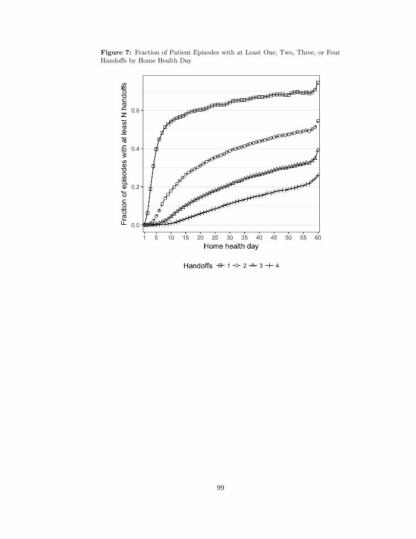
Figure 7: Fraction of Patient Episodes with at Least One, Two, Three, or FourHandoffs by Home Health Day
99
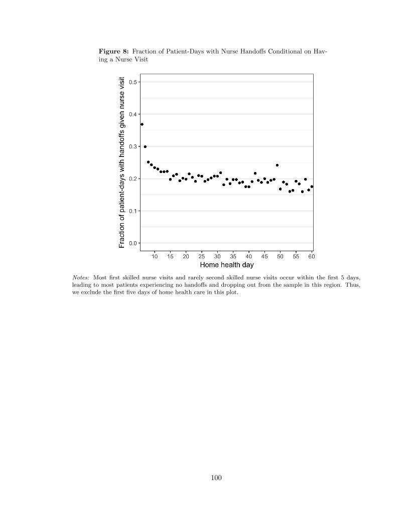
Figure 8: Fraction of Patient-Days with Nurse Handoffs Conditional on Hav-ing a Nurse Visit
Notes: Most first skilled nurse visits and rarely second skilled nurse visits occur within the first 5 days,leading to most patients experiencing no handoffs and dropping out from the sample in this region. Thus,we exclude the first five days of home health care in this plot.
100
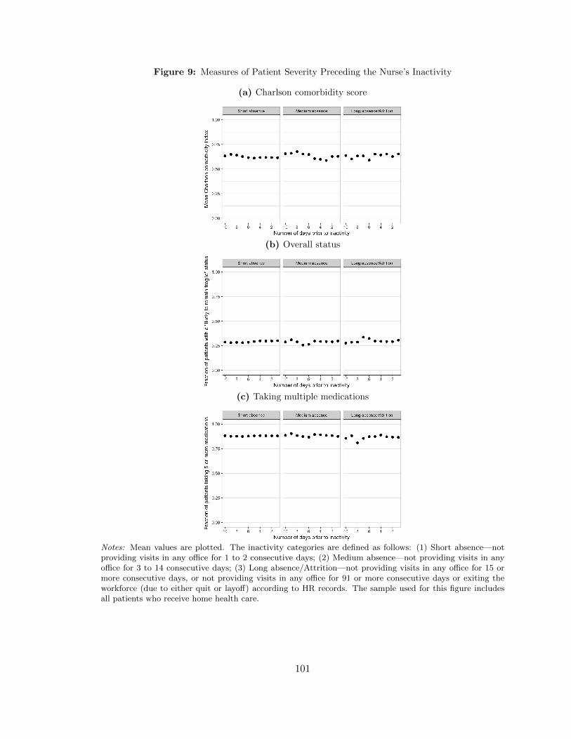
Figure 9: Measures of Patient Severity Preceding the Nurse’s Inactivity
(a) Charlson comorbidity score
(b) Overall status
(c) Taking multiple medications
Notes: Mean values are plotted. The inactivity categories are defined as follows: (1) Short absence—notproviding visits in any office for 1 to 2 consecutive days; (2) Medium absence—not providing visits in anyoffice for 3 to 14 consecutive days; (3) Long absence/Attrition—not providing visits in any office for 15 ormore consecutive days, or not providing visits in any office for 91 or more consecutive days or exiting theworkforce (due to either quit or layoff) according to HR records. The sample used for this figure includesall patients who receive home health care.
101
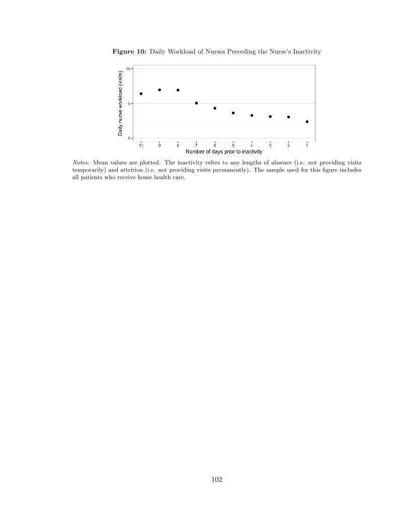
Figure 10: Daily Workload of Nurses Preceding the Nurse’s Inactivity
Notes: Mean values are plotted. The inactivity refers to any lengths of absence (i.e. not providing visitstemporarily) and attrition (i.e. not providing visits permanently). The sample used for this figure includesall patients who receive home health care.
102

Figure 11: Daily Office Caseload Before and After the Nurse’s Inactivity
(a) Daily number of ongoing episodes
(b) Daily number of new episodes
(c) Daily number of nurse visits
Notes: Mean values are plotted. The inactivity refers to any lengths of absence (i.e. not providing visitstemporarily). The sample used for this figure includes all patients who receive home health care.
103

Table 14: Sample Summary Statistics for the Sample Period 2012–2015
Variables Mean Std Dev
A. Office-day-level variables (Number of observations = 92,676)Number of ongoing episodes 113.098 68.345Number of active nurses 14.596 10.908
B. Patient episode-level variables (Number of observations = 43,740)Hospital readmission 0.166 0.372Hospital readmission within 30 days of hospital discharge 0.130 0.337Death 0.003 0.053Length of episode (in days) 32.672 16.268Number of nurse visits 5.791 3.067Number of nurse handoffs 1.327 1.600Mean number of days between nurse visits 5.251 2.948Age 78.961 8.423Female 0.598 0.490White 0.820 0.384Living alone 0.234 0.423No assistance available 0.017 0.131Enrolled in per-visit paying Medicare Advantage 0.190 0.393Enrolled in per-episode paying Medicare Advantage 0.062 0.242Dual eligible 0.006 0.078Risk for hospitalization: History of 2+ falls 0.255 0.436Risk for hospitalization: 2+ hospitalizations 0.372 0.483Risk for hospitalization: Recent decline in Mental 0.068 0.251Risk for hospitalization: Take 5+ medications 0.872 0.334Risk for hospitalization: Other 0.091 0.288Acute myocardial infarction (AMI) 0.022 0.148Congestive heart failure (CHF) 0.130 0.336Peripheral vascular disease (PVD) 0.016 0.125Cerebrovascular disease (CEVD) 0.051 0.220Dementia 0.007 0.084Chronic pulmonary disease (COPD) 0.104 0.305Rheumatic disease 0.001 0.030Peptic ulcer disease 0.003 0.055Mild liver disease 0.004 0.065Diabetes 0.017 0.129Diabetes + Complications 0.009 0.096Hemiplegia or paraplegia (HP/PAPL) 0.002 0.048Renal disease 0.029 0.169Cancer 0.070 0.255Moderate/severe liver disease 0.002 0.045Metastatic cancer 0.008 0.089AIDS/HIV 0.000 0.011Overall status: (Very bad) Progressive conditions 0.033 0.179Overall status: (Bad) Remain in fragile health 0.274 0.446Overall status: Temporarily facing high health risks 0.615 0.487High risk factor: Alcohol dependency 0.024 0.154High risk factor: Drug dependency 0.007 0.083High risk factor: Heavy smoking 0.133 0.340High risk factor: Obesity 0.163 0.369
104
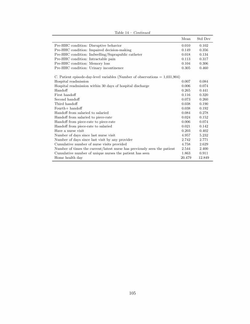
Table 14 – Continued
Mean Std Dev
Pre-HHC condition: Disruptive behavior 0.010 0.102Pre-HHC condition: Impaired decision-making 0.149 0.356Pre-HHC condition: Indwelling/Suprapublic catheter 0.018 0.134Pre-HHC condition: Intractable pain 0.113 0.317Pre-HHC condition: Memory loss 0.104 0.306Pre-HHC condition: Urinary incontinence 0.305 0.460
C. Patient episode-day-level variables (Number of observations = 1,031,904)Hospital readmission 0.007 0.084Hospital readmission within 30 days of hospital discharge 0.006 0.074Handoff 0.265 0.441First handoff 0.116 0.320Second handoff 0.073 0.260Third handoff 0.038 0.190Fourth+ handoff 0.038 0.192Handoff from salaried to salaried 0.084 0.278Handoff from salaried to piece-rate 0.024 0.152Handoff from piece-rate to piece-rate 0.006 0.074Handoff from piece-rate to salaried 0.021 0.142Have a nurse visit 0.203 0.402Number of days since last nurse visit 4.957 5.232Number of days since last visit by any provider 2.742 2.771Cumulative number of nurse visits provided 4.758 2.629Number of times the current/latest nurse has previously seen the patient 2.544 2.400Cumulative number of unique nurses the patient has seen 1.863 0.911Home health day 20.479 12.849
105
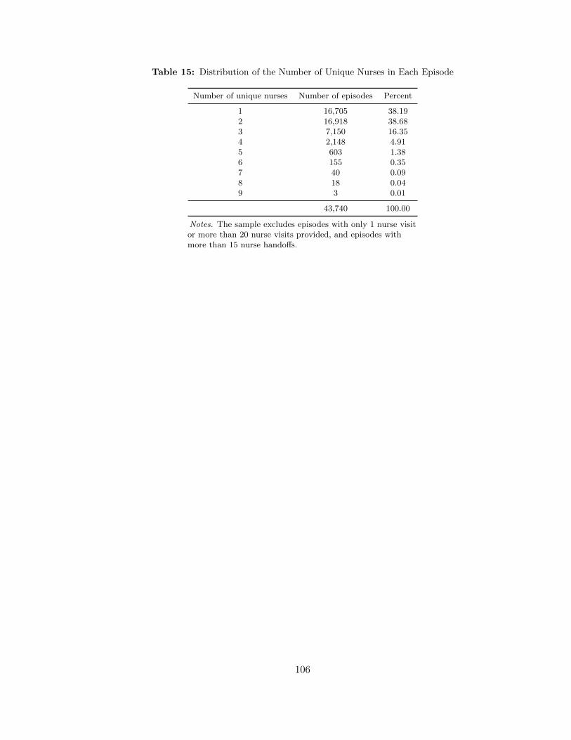
Table 15: Distribution of the Number of Unique Nurses in Each Episode
Number of unique nurses Number of episodes Percent
1 16,705 38.192 16,918 38.683 7,150 16.354 2,148 4.915 603 1.386 155 0.357 40 0.098 18 0.049 3 0.01
43,740 100.00
Notes. The sample excludes episodes with only 1 nurse visitor more than 20 nurse visits provided, and episodes withmore than 15 nurse handoffs.
106

Table 16: Distribution of Patient-Day Observations and the Likelihood ofNurse Handoff, Nurse Visit, and Readmission by the Availability of Nurse WhoVisited a Patient in the Last Visit
N Obs % Obs % Handoff % Have a nurse visit % Readmission
Active 670,621 64.99 20.63 27.37 0.77Short absence (1-6 days) 290,098 28.11 31.07 6.20 0.56Medium absence (7-14 days) 32,232 3.12 62.45 11.94 0.67Long absence (15+ days) 13,834 1.34 73.28 11.41 0.71Assigned to other office 13,415 1.30 49.30 11.20 0.83Attrition 11,704 1.13 65.02 9.28 0.67
Total 1,031,904 100.00
Notes. In the entire sample of patient-day observations, the percentage of handoff is 26.46%; the percent-age of having a nurse visit is 20.31%; the percentage of readmission is 0.71%.
107

Table 17: OLS: Patients Experiencing a Handoff Are More Likely to Be Re-hospitalized
Dep Var: Indicator for being rehospitalized(1) (2) (3) (4)
Handoff 0.0017*** 0.0017*** 0.0017*** 0.0017***(0.0002) (0.0002) (0.0002) (0.0002)
R-squared 0.0067 0.0072 0.0073 0.0081Observations 1,031,904 1,031,904 1,031,904 1,031,904Hospitalization risk controls . Yes Yes YesDemographic controls . . Yes YesComorbidity controls . . . Yes
Notes. This table presents linear probability models examining whether patients experiencing a handoff are morelikely to be rehospitalized. An observation is a patient episode-day. Robust standard errors allowing for arbitrarycorrelation among episode-days in the same office in parentheses. In all panels and all columns, we control for theindicator for having a nurse visit, cumulative number of nurse visits provided, mean interval of days between twoconsecutive visits during the episode, number of days since last nurse visit, number of days since last visit by anyprovider; number of ongoing episodes in the office-day, number of nurses working in the office-day; and office fixedeffects, day of week fixed effects, month-year of the day fixed effects, and home health day fixed effects. In columns(2)-(4), hospitalization risk controls include dummies for the risk factors for hospitalization: history of 2+ falls inthe past 12 months; 2+ hospitalizations in the past 6 months; decline in mental, emotional, or behavioral status inthe past 3 months, currently taking 5+ medications, and others. In columns (3)-(4), demographic controls includeage dummies for each age 66-94 and age 95+ (reference group: age=65); female; white; insurance type–MedicareAdvantage (MA) plan with a visit-based reimbursement, MA plan with an episode-based reimbursement, dual eligi-ble with Medicaid enrollment (reference group: Medicare FFS); dummy for having no assistance available; dummyfor living alone. In column (4), comorbidity controls include dummies for 17 Charlson comorbidity index factors;dummies overall status–very bad (patient has serious progressive conditions that could lead to death within a year),bad (patient is likely to remain in fragile health); and temporarily bad (temporary facing high health risks); dum-mies for high-risk factors–alcohol dependency, drug dependency, smoking, obesity–and dummies for conditions priorto hospital stay within past 14 days–disruptive or socially inappropriate behavior, impaired decision making, in-dwelling or suprapublic catheter, intractable pain, serious memory loss, urinary incontinence. *significant at 10%;**significant at 5%; ***significant at 1%.
108
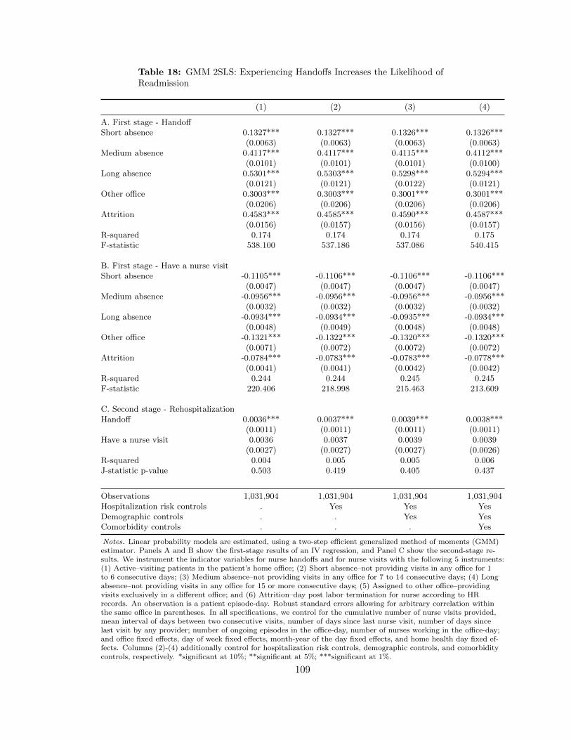
Table 18: GMM 2SLS: Experiencing Handoffs Increases the Likelihood ofReadmission
(1) (2) (3) (4)
A. First stage - HandoffShort absence 0.1327*** 0.1327*** 0.1326*** 0.1326***
(0.0063) (0.0063) (0.0063) (0.0063)Medium absence 0.4117*** 0.4117*** 0.4115*** 0.4112***
(0.0101) (0.0101) (0.0101) (0.0100)Long absence 0.5301*** 0.5303*** 0.5298*** 0.5294***
(0.0121) (0.0121) (0.0122) (0.0121)Other office 0.3003*** 0.3003*** 0.3001*** 0.3001***
(0.0206) (0.0206) (0.0206) (0.0206)Attrition 0.4583*** 0.4585*** 0.4590*** 0.4587***
(0.0156) (0.0157) (0.0156) (0.0157)R-squared 0.174 0.174 0.174 0.175F-statistic 538.100 537.186 537.086 540.415
B. First stage - Have a nurse visitShort absence -0.1105*** -0.1106*** -0.1106*** -0.1106***
(0.0047) (0.0047) (0.0047) (0.0047)Medium absence -0.0956*** -0.0956*** -0.0956*** -0.0956***
(0.0032) (0.0032) (0.0032) (0.0032)Long absence -0.0934*** -0.0934*** -0.0935*** -0.0934***
(0.0048) (0.0049) (0.0048) (0.0048)Other office -0.1321*** -0.1322*** -0.1320*** -0.1320***
(0.0071) (0.0072) (0.0072) (0.0072)Attrition -0.0784*** -0.0783*** -0.0783*** -0.0778***
(0.0041) (0.0041) (0.0042) (0.0042)R-squared 0.244 0.244 0.245 0.245F-statistic 220.406 218.998 215.463 213.609
C. Second stage - RehospitalizationHandoff 0.0036*** 0.0037*** 0.0039*** 0.0038***
(0.0011) (0.0011) (0.0011) (0.0011)Have a nurse visit 0.0036 0.0037 0.0039 0.0039
(0.0027) (0.0027) (0.0027) (0.0026)R-squared 0.004 0.005 0.005 0.006J-statistic p-value 0.503 0.419 0.405 0.437
Observations 1,031,904 1,031,904 1,031,904 1,031,904Hospitalization risk controls . Yes Yes YesDemographic controls . . Yes YesComorbidity controls . . . Yes
Notes. Linear probability models are estimated, using a two-step efficient generalized method of moments (GMM)estimator. Panels A and B show the first-stage results of an IV regression, and Panel C show the second-stage re-sults. We instrument the indicator variables for nurse handoffs and for nurse visits with the following 5 instruments:(1) Active–visiting patients in the patient’s home office; (2) Short absence–not providing visits in any office for 1to 6 consecutive days; (3) Medium absence–not providing visits in any office for 7 to 14 consecutive days; (4) Longabsence–not providing visits in any office for 15 or more consecutive days; (5) Assigned to other office–providingvisits exclusively in a different office; and (6) Attrition–day post labor termination for nurse according to HRrecords. An observation is a patient episode-day. Robust standard errors allowing for arbitrary correlation withinthe same office in parentheses. In all specifications, we control for the cumulative number of nurse visits provided,mean interval of days between two consecutive visits, number of days since last nurse visit, number of days sincelast visit by any provider; number of ongoing episodes in the office-day, number of nurses working in the office-day;and office fixed effects, day of week fixed effects, month-year of the day fixed effects, and home health day fixed ef-fects. Columns (2)-(4) additionally control for hospitalization risk controls, demographic controls, and comorbiditycontrols, respectively. *significant at 10%; **significant at 5%; ***significant at 1%.
109
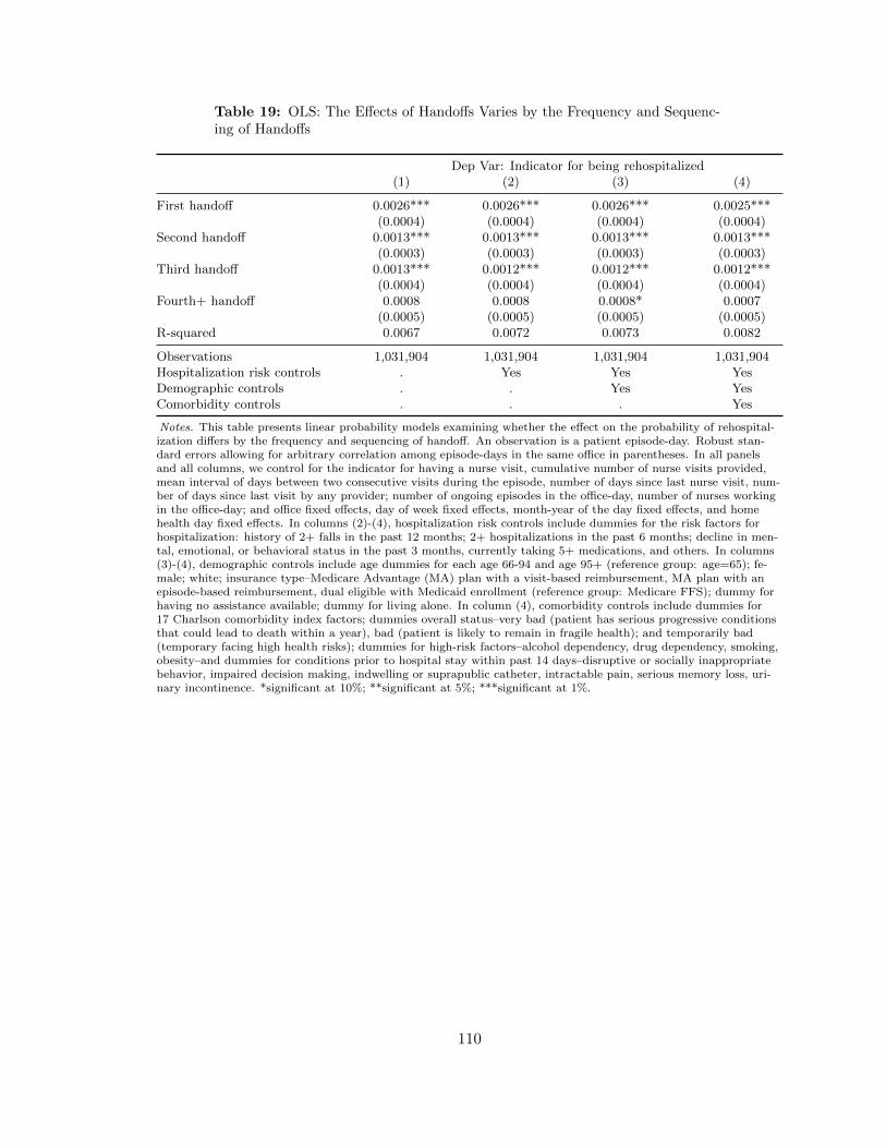
Table 19: OLS: The Effects of Handoffs Varies by the Frequency and Sequenc-ing of Handoffs
Dep Var: Indicator for being rehospitalized(1) (2) (3) (4)
First handoff 0.0026*** 0.0026*** 0.0026*** 0.0025***(0.0004) (0.0004) (0.0004) (0.0004)
Second handoff 0.0013*** 0.0013*** 0.0013*** 0.0013***(0.0003) (0.0003) (0.0003) (0.0003)
Third handoff 0.0013*** 0.0012*** 0.0012*** 0.0012***(0.0004) (0.0004) (0.0004) (0.0004)
Fourth+ handoff 0.0008 0.0008 0.0008* 0.0007(0.0005) (0.0005) (0.0005) (0.0005)
R-squared 0.0067 0.0072 0.0073 0.0082
Observations 1,031,904 1,031,904 1,031,904 1,031,904Hospitalization risk controls . Yes Yes YesDemographic controls . . Yes YesComorbidity controls . . . Yes
Notes. This table presents linear probability models examining whether the effect on the probability of rehospital-ization differs by the frequency and sequencing of handoff. An observation is a patient episode-day. Robust stan-dard errors allowing for arbitrary correlation among episode-days in the same office in parentheses. In all panelsand all columns, we control for the indicator for having a nurse visit, cumulative number of nurse visits provided,mean interval of days between two consecutive visits during the episode, number of days since last nurse visit, num-ber of days since last visit by any provider; number of ongoing episodes in the office-day, number of nurses workingin the office-day; and office fixed effects, day of week fixed effects, month-year of the day fixed effects, and homehealth day fixed effects. In columns (2)-(4), hospitalization risk controls include dummies for the risk factors forhospitalization: history of 2+ falls in the past 12 months; 2+ hospitalizations in the past 6 months; decline in men-tal, emotional, or behavioral status in the past 3 months, currently taking 5+ medications, and others. In columns(3)-(4), demographic controls include age dummies for each age 66-94 and age 95+ (reference group: age=65); fe-male; white; insurance type–Medicare Advantage (MA) plan with a visit-based reimbursement, MA plan with anepisode-based reimbursement, dual eligible with Medicaid enrollment (reference group: Medicare FFS); dummy forhaving no assistance available; dummy for living alone. In column (4), comorbidity controls include dummies for17 Charlson comorbidity index factors; dummies overall status–very bad (patient has serious progressive conditionsthat could lead to death within a year), bad (patient is likely to remain in fragile health); and temporarily bad(temporary facing high health risks); dummies for high-risk factors–alcohol dependency, drug dependency, smoking,obesity–and dummies for conditions prior to hospital stay within past 14 days–disruptive or socially inappropriatebehavior, impaired decision making, indwelling or suprapublic catheter, intractable pain, serious memory loss, uri-nary incontinence. *significant at 10%; **significant at 5%; ***significant at 1%.
110
3.6. Appendix
3.6.1. Analysis Using the 30-Day Readmission Outcome
We report the OLS and 2SLS results estimated using the indicator for rehospitalizationwithin 30 days of hospital discharge in Tables 20 and 21, respectively. We find that thecoefficient estimates remain similar, albeit slightly lower in the OLS estimation result andhigher in the IV estimation result. The similar size in estimates is not surprising sinceTable 14 shows that most of the hospital readmission occurs within 30 days of hospitaldischarge. The IV estimates in Table 21 imply that experiencing a handoff increases theprobability of readmission by 0.42–0.47 percentage points (70–78%). The higher percentagechanges in this result result from a lower 30-day readmission rate (13%) than the all-timereadmission rate (17%).
111
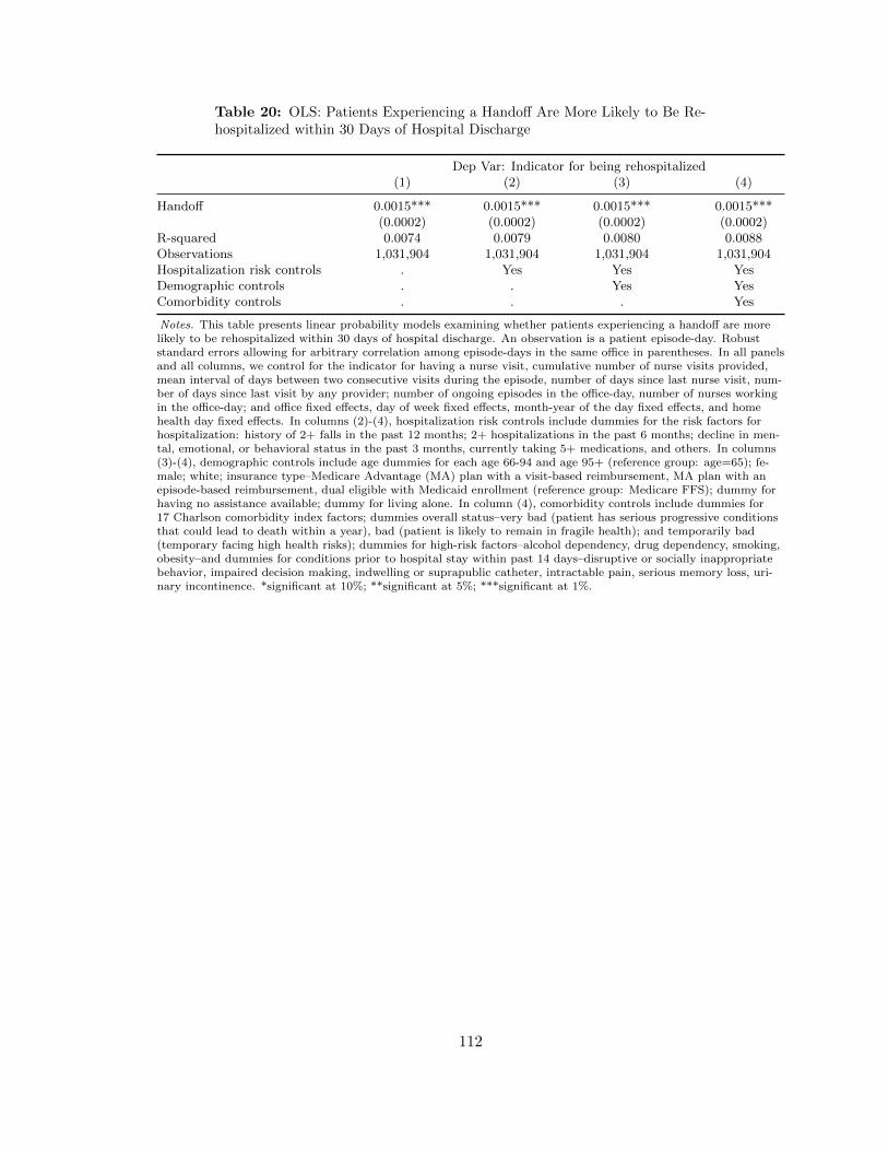
Table 20: OLS: Patients Experiencing a Handoff Are More Likely to Be Re-hospitalized within 30 Days of Hospital Discharge
Dep Var: Indicator for being rehospitalized(1) (2) (3) (4)
Handoff 0.0015*** 0.0015*** 0.0015*** 0.0015***(0.0002) (0.0002) (0.0002) (0.0002)
R-squared 0.0074 0.0079 0.0080 0.0088Observations 1,031,904 1,031,904 1,031,904 1,031,904Hospitalization risk controls . Yes Yes YesDemographic controls . . Yes YesComorbidity controls . . . Yes
Notes. This table presents linear probability models examining whether patients experiencing a handoff are morelikely to be rehospitalized within 30 days of hospital discharge. An observation is a patient episode-day. Robuststandard errors allowing for arbitrary correlation among episode-days in the same office in parentheses. In all panelsand all columns, we control for the indicator for having a nurse visit, cumulative number of nurse visits provided,mean interval of days between two consecutive visits during the episode, number of days since last nurse visit, num-ber of days since last visit by any provider; number of ongoing episodes in the office-day, number of nurses workingin the office-day; and office fixed effects, day of week fixed effects, month-year of the day fixed effects, and homehealth day fixed effects. In columns (2)-(4), hospitalization risk controls include dummies for the risk factors forhospitalization: history of 2+ falls in the past 12 months; 2+ hospitalizations in the past 6 months; decline in men-tal, emotional, or behavioral status in the past 3 months, currently taking 5+ medications, and others. In columns(3)-(4), demographic controls include age dummies for each age 66-94 and age 95+ (reference group: age=65); fe-male; white; insurance type–Medicare Advantage (MA) plan with a visit-based reimbursement, MA plan with anepisode-based reimbursement, dual eligible with Medicaid enrollment (reference group: Medicare FFS); dummy forhaving no assistance available; dummy for living alone. In column (4), comorbidity controls include dummies for17 Charlson comorbidity index factors; dummies overall status–very bad (patient has serious progressive conditionsthat could lead to death within a year), bad (patient is likely to remain in fragile health); and temporarily bad(temporary facing high health risks); dummies for high-risk factors–alcohol dependency, drug dependency, smoking,obesity–and dummies for conditions prior to hospital stay within past 14 days–disruptive or socially inappropriatebehavior, impaired decision making, indwelling or suprapublic catheter, intractable pain, serious memory loss, uri-nary incontinence. *significant at 10%; **significant at 5%; ***significant at 1%.
112

Table 21: GMM 2SLS: Experiencing Handoffs Increases the Likelihood ofReadmission within 30 Days of Hospital Discharge
(1) (2) (3) (4)
A. First stage - HandoffShort absence 0.0879*** 0.0879*** 0.0879*** 0.0880***
(0.0047) (0.0047) (0.0047) (0.0047)Medium absence 0.2707*** 0.2707*** 0.2706*** 0.2706***
(0.0076) (0.0076) (0.0075) (0.0075)Long absence 0.3462*** 0.3463*** 0.3462*** 0.3460***
(0.0104) (0.0104) (0.0104) (0.0104)Other office 0.2112*** 0.2113*** 0.2111*** 0.2112***
(0.0143) (0.0143) (0.0144) (0.0143)Attrition 0.2763*** 0.2764*** 0.2767*** 0.2767***
(0.0118) (0.0118) (0.0118) (0.0117)R-squared 0.430 0.430 0.430 0.430F-statistic 389.119 389.243 393.149 395.680
B. First stage - Have a nurse visitShort absence -0.1115*** -0.1116*** -0.1116*** -0.1116***
(0.0047) (0.0047) (0.0047) (0.0048)Medium absence -0.0981*** -0.0982*** -0.0981*** -0.0982***
(0.0033) (0.0033) (0.0033) (0.0033)Long absence -0.0972*** -0.0972*** -0.0973*** -0.0973***
(0.0050) (0.0050) (0.0050) (0.0050)Other office -0.1344*** -0.1345*** -0.1343*** -0.1343***
(0.0071) (0.0071) (0.0071) (0.0071)Attrition -0.0816*** -0.0814*** -0.0815*** -0.0810***
(0.0041) (0.0042) (0.0042) (0.0042)R-squared 0.245 0.245 0.245 0.245F-statistic 222.072 220.780 216.391 214.325
C. Second stage - 30-day rehospitalizationHandoff 0.0042*** 0.0044*** 0.0046*** 0.0047***
(0.0016) (0.0016) (0.0016) (0.0016)Have a nurse visit 0.0044* 0.0046* 0.0047* 0.0047*
(0.0026) (0.0026) (0.0026) (0.0026)R-squared 0.004 0.004 0.004 0.005J-statistic p-value 0.744 0.669 0.650 0.742
Observations 1,031,904 1,031,904 1,031,904 1,031,904Hospitalization risk controls . Yes Yes YesDemographic controls . . Yes YesComorbidity controls . . . Yes
Notes. Linear probability models are estimated, using a two-step efficient generalized method of moments (GMM)estimator. Panels A and B show the first-stage results of an IV regression, and Panel C show the second-stage re-sults. We instrument the indicator variables for nurse handoffs and for nurse visits with the following 5 instruments:(1) Active–visiting patients in the patient’s home office; (2) Short absence–not providing visits in any office for 1to 6 consecutive days; (3) Medium absence–not providing visits in any office for 7 to 14 consecutive days; (4) Longabsence–not providing visits in any office for 15 or more consecutive days; (5) Assigned to other office–providingvisits exclusively in a different office; and (6) Attrition–day post labor termination for nurse according to HRrecords. An observation is a patient episode-day. Robust standard errors allowing for arbitrary correlation withinthe same office in parentheses. In all specifications, we control for the cumulative number of nurse visits provided,mean interval of days between two consecutive visits, number of days since last nurse visit, number of days sincelast visit by any provider; number of ongoing episodes in the office-day, number of nurses working in the office-day;and office fixed effects, day of week fixed effects, month-year of the day fixed effects, and home health day fixed ef-fects. Columns (2)-(4) additionally control for hospitalization risk controls, demographic controls, and comorbiditycontrols, respectively. *significant at 10%; **significant at 5%; ***significant at 1%.
113
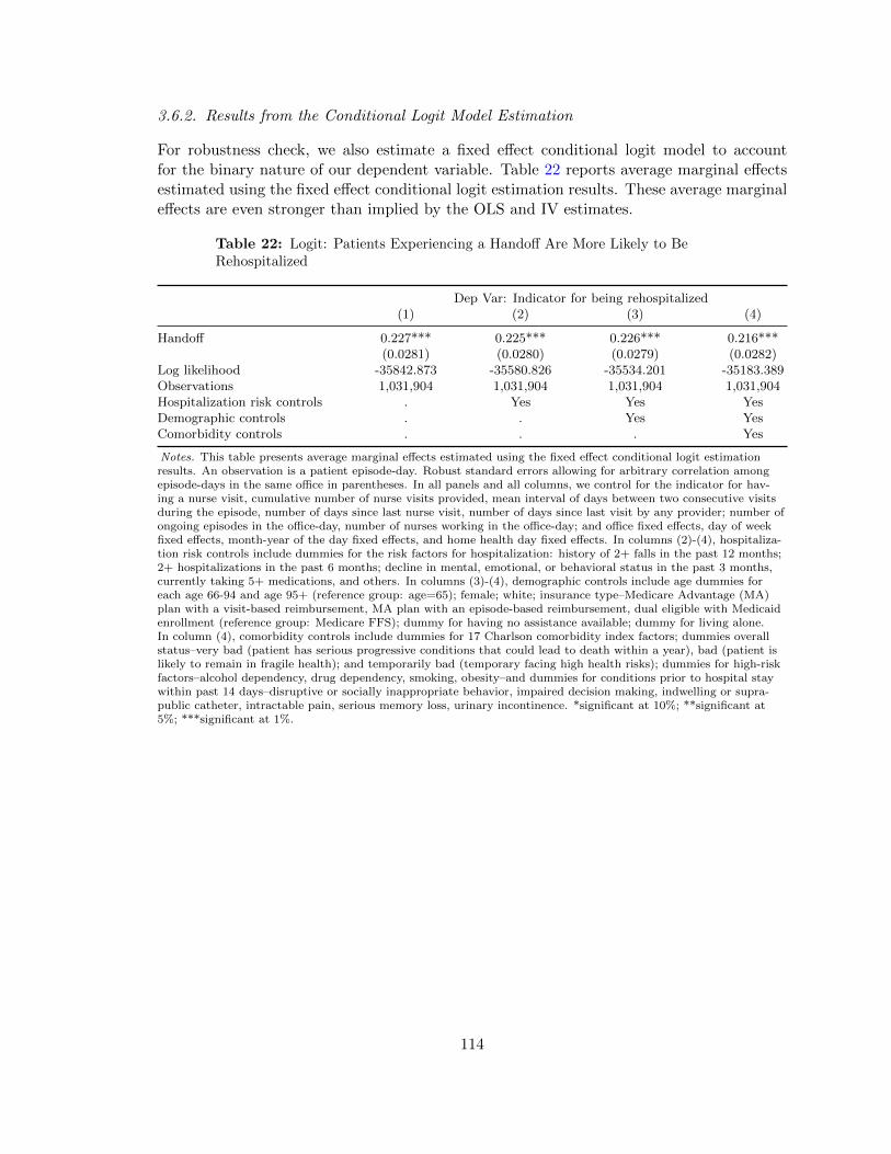
3.6.2. Results from the Conditional Logit Model Estimation
For robustness check, we also estimate a fixed effect conditional logit model to accountfor the binary nature of our dependent variable. Table 22 reports average marginal effectsestimated using the fixed effect conditional logit estimation results. These average marginaleffects are even stronger than implied by the OLS and IV estimates.
Table 22: Logit: Patients Experiencing a Handoff Are More Likely to BeRehospitalized
Dep Var: Indicator for being rehospitalized(1) (2) (3) (4)
Handoff 0.227*** 0.225*** 0.226*** 0.216***(0.0281) (0.0280) (0.0279) (0.0282)
Log likelihood -35842.873 -35580.826 -35534.201 -35183.389Observations 1,031,904 1,031,904 1,031,904 1,031,904Hospitalization risk controls . Yes Yes YesDemographic controls . . Yes YesComorbidity controls . . . Yes
Notes. This table presents average marginal effects estimated using the fixed effect conditional logit estimationresults. An observation is a patient episode-day. Robust standard errors allowing for arbitrary correlation amongepisode-days in the same office in parentheses. In all panels and all columns, we control for the indicator for hav-ing a nurse visit, cumulative number of nurse visits provided, mean interval of days between two consecutive visitsduring the episode, number of days since last nurse visit, number of days since last visit by any provider; number ofongoing episodes in the office-day, number of nurses working in the office-day; and office fixed effects, day of weekfixed effects, month-year of the day fixed effects, and home health day fixed effects. In columns (2)-(4), hospitaliza-tion risk controls include dummies for the risk factors for hospitalization: history of 2+ falls in the past 12 months;2+ hospitalizations in the past 6 months; decline in mental, emotional, or behavioral status in the past 3 months,currently taking 5+ medications, and others. In columns (3)-(4), demographic controls include age dummies foreach age 66-94 and age 95+ (reference group: age=65); female; white; insurance type–Medicare Advantage (MA)plan with a visit-based reimbursement, MA plan with an episode-based reimbursement, dual eligible with Medicaidenrollment (reference group: Medicare FFS); dummy for having no assistance available; dummy for living alone.In column (4), comorbidity controls include dummies for 17 Charlson comorbidity index factors; dummies overallstatus–very bad (patient has serious progressive conditions that could lead to death within a year), bad (patient islikely to remain in fragile health); and temporarily bad (temporary facing high health risks); dummies for high-riskfactors–alcohol dependency, drug dependency, smoking, obesity–and dummies for conditions prior to hospital staywithin past 14 days–disruptive or socially inappropriate behavior, impaired decision making, indwelling or supra-public catheter, intractable pain, serious memory loss, urinary incontinence. *significant at 10%; **significant at5%; ***significant at 1%.
114

3.6.3. Correlation of Selected Measures of Patients’ Severity and Rehospitalization
Table 23 presents coefficient estimates on three selected measures of patients’ severity—indicators for each category of Charlson comorbidity index, overall status likely to remainfragile, and taking 5 or more medications—obtained from estimating the model in Column(4) of Table 17. We find that reported severity measures are statistically significant andstrong predictors of the likelihood of readmission, even stronger than handoff.
115

Table 23: Key Measures of Patients’ Severity as Predictors of the Likelihood ofReadmission
Dep Var: Indicator for being rehospitalized
Handoff 0.0017***(0.0002)
A. 17 Components of the Charlson Comorbidity IndexAcute myocardial infarction (AMI) 0.0001
(0.0007)Congestive heart failure (CHF) 0.0028***
(0.0003)Peripheral vascular disease (PVD) 0.0026***
(0.0009)Cerebrovascular disease (CEVD) 0.0008**
(0.0003)Dementia 0.0018*
(0.0011)Chronic pulmonary disease (COPD) 0.0023***
(0.0004)Rheumatic disease 0.0008
(0.0025)Peptic ulcer disease 0.0052**
(0.0020)Mild liver disease 0.0016
(0.0016)Diabetes 0.0014**
(0.0007)Diabetes + Complications 0.0057***
(0.0013)Hemiplegia or paraplegia (HP/PAPL) 0.0002
(0.0017)Renal disease 0.0032***
(0.0007)Cancer 0.0041***
(0.0005)Moderate/severe liver disease 0.0067***
(0.0024)Metastatic cancer 0.0045***
(0.0015)AIDS/HIV 0.0107
(0.0115)
B. Overall StatusLikely to remain in fragile health 0.0034***
(0.0004)
C. Risk for HospitalizationTake 5 or more medications 0.0005*
(0.0003)R-squared 0.0081Observations 1,031,904
Notes. An observation is a patient episode-day. Robust standard errors allowing for ar-bitrary correlation among episode-days in the same office in parentheses. *significant at10%; **significant at 5%; ***significant at 1%.
116
3.6.4. Robustness Check Using an Alternative Definition of Breaks in Nurses’ Availability
In this appendix, we run a robustness check on our main IV results using an alternativedefinition of medium absence. We define medium absence as not providing visits in anyoffice for 6 to 20 consecutive days, and accordingly, short absence for 1 to 5 consecutivedays and long absence for 21 or more consecutive days.
Table 24 presents the distribution of the number of patient episode-day observations as wellas the likelihood of having a provider handoff, a nurse visit, and a hospital readmission foreach newly defined availability category. The distributions of observations and probabili-ties of handoffs, nurse visits, and readmissions change little when we use a wider windowof time for medium absence. A noticeable difference is an increase in the probabilities ofhandoffs and readmissions when a provider is having a long absence under the new defini-tion. However, qualitatively, the relative orders of these numbers remain the same acrossthe categories. Therefore, we obtain very similar first-stage and second-stage estimates inTable 25 to those in Table 18. In Panels A and B for the first-stage results, each of providers’unavailability status seems to be a stronger predictor of patients’ handoffs and a slightlyweaker predictor of patients’ receiving nurse visits. However, the F-statistic values are stillsignificantly large. In Panel C, in Column (4), we find a tiny decrease in the magnitude ofthe effect of experiencing a handoff at 0.37 percentage points or 53% on the likelihood ofrehospitalization.
117

Table 24: Distribution of Patient-Day Observations and the Likelihood ofNurse Handoff, Nurse Visit, and Readmission by the Availability of Nurse WhoVisited a Patient in the Last Visit
N Obs % Obs % Handoff % Have a nurse visit % Readmission
Active 670,621 64.99 20.63 27.37 0.77Short absence (1-5 days) 280,872 27.22 29.95 5.94 0.55Medium absence (6-20 days) 47,559 4.61 63.72 12.22 0.70Long absence (21+ days) 7,733 0.75 77.42 11.95 0.72Assigned to other office 13,415 1.30 49.30 11.20 0.83Attrition 11,704 1.13 65.02 9.28 0.67
Total 1,031,904 100.00
Notes. In the entire sample of patient-day observations, the percentage of handoff is 26.46%; the percent-age of having a nurse visit is 20.31%; the percentage of readmission is 0.71%.
118
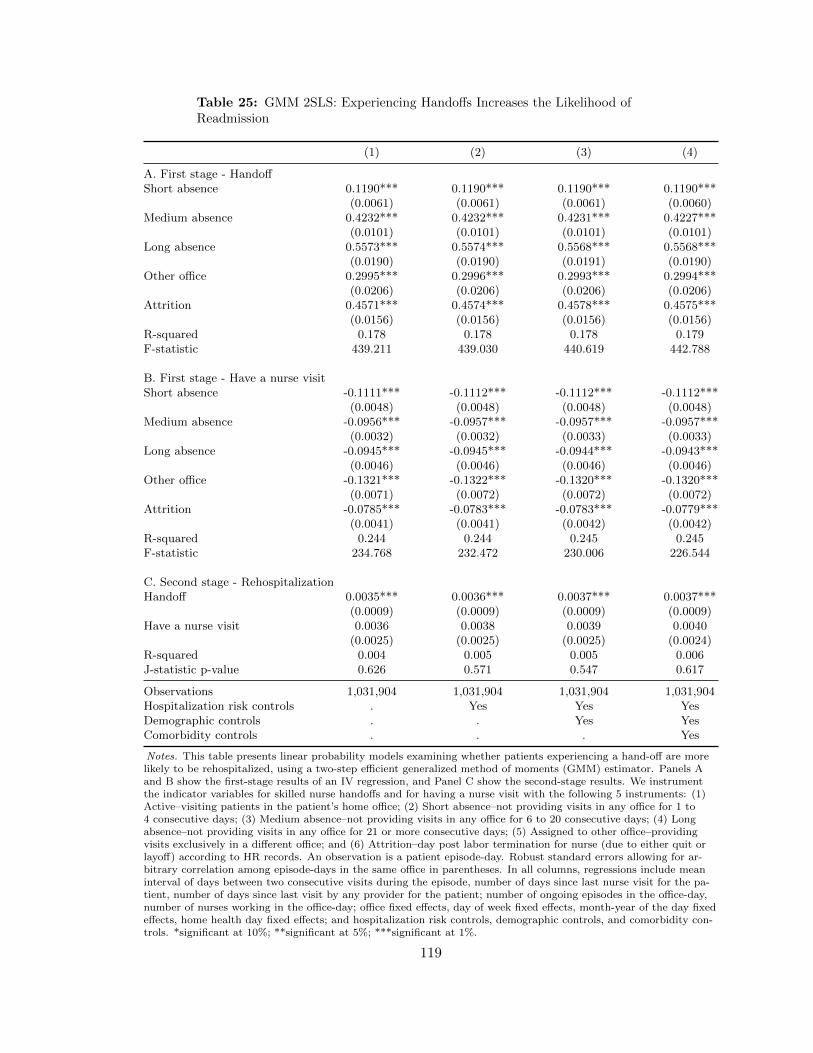
Table 25: GMM 2SLS: Experiencing Handoffs Increases the Likelihood ofReadmission
(1) (2) (3) (4)
A. First stage - HandoffShort absence 0.1190*** 0.1190*** 0.1190*** 0.1190***
(0.0061) (0.0061) (0.0061) (0.0060)Medium absence 0.4232*** 0.4232*** 0.4231*** 0.4227***
(0.0101) (0.0101) (0.0101) (0.0101)Long absence 0.5573*** 0.5574*** 0.5568*** 0.5568***
(0.0190) (0.0190) (0.0191) (0.0190)Other office 0.2995*** 0.2996*** 0.2993*** 0.2994***
(0.0206) (0.0206) (0.0206) (0.0206)Attrition 0.4571*** 0.4574*** 0.4578*** 0.4575***
(0.0156) (0.0156) (0.0156) (0.0156)R-squared 0.178 0.178 0.178 0.179F-statistic 439.211 439.030 440.619 442.788
B. First stage - Have a nurse visitShort absence -0.1111*** -0.1112*** -0.1112*** -0.1112***
(0.0048) (0.0048) (0.0048) (0.0048)Medium absence -0.0956*** -0.0957*** -0.0957*** -0.0957***
(0.0032) (0.0032) (0.0033) (0.0033)Long absence -0.0945*** -0.0945*** -0.0944*** -0.0943***
(0.0046) (0.0046) (0.0046) (0.0046)Other office -0.1321*** -0.1322*** -0.1320*** -0.1320***
(0.0071) (0.0072) (0.0072) (0.0072)Attrition -0.0785*** -0.0783*** -0.0783*** -0.0779***
(0.0041) (0.0041) (0.0042) (0.0042)R-squared 0.244 0.244 0.245 0.245F-statistic 234.768 232.472 230.006 226.544
C. Second stage - RehospitalizationHandoff 0.0035*** 0.0036*** 0.0037*** 0.0037***
(0.0009) (0.0009) (0.0009) (0.0009)Have a nurse visit 0.0036 0.0038 0.0039 0.0040
(0.0025) (0.0025) (0.0025) (0.0024)R-squared 0.004 0.005 0.005 0.006J-statistic p-value 0.626 0.571 0.547 0.617
Observations 1,031,904 1,031,904 1,031,904 1,031,904Hospitalization risk controls . Yes Yes YesDemographic controls . . Yes YesComorbidity controls . . . Yes
Notes. This table presents linear probability models examining whether patients experiencing a hand-off are morelikely to be rehospitalized, using a two-step efficient generalized method of moments (GMM) estimator. Panels Aand B show the first-stage results of an IV regression, and Panel C show the second-stage results. We instrumentthe indicator variables for skilled nurse handoffs and for having a nurse visit with the following 5 instruments: (1)Active–visiting patients in the patient’s home office; (2) Short absence–not providing visits in any office for 1 to4 consecutive days; (3) Medium absence–not providing visits in any office for 6 to 20 consecutive days; (4) Longabsence–not providing visits in any office for 21 or more consecutive days; (5) Assigned to other office–providingvisits exclusively in a different office; and (6) Attrition–day post labor termination for nurse (due to either quit orlayoff) according to HR records. An observation is a patient episode-day. Robust standard errors allowing for ar-bitrary correlation among episode-days in the same office in parentheses. In all columns, regressions include meaninterval of days between two consecutive visits during the episode, number of days since last nurse visit for the pa-tient, number of days since last visit by any provider for the patient; number of ongoing episodes in the office-day,number of nurses working in the office-day; office fixed effects, day of week fixed effects, month-year of the day fixedeffects, home health day fixed effects; and hospitalization risk controls, demographic controls, and comorbidity con-trols. *significant at 10%; **significant at 5%; ***significant at 1%.
119
APPENDIX
A.1. Home Health Care Industry
Home health care, which is provided to homebound patients who need skilled nursing or
therapy services, is an important and rapidly growing segment of the post-acute care delivery
system. The number of home health agencies (HHAs), which are the major providers of
home health care, had grown from 9,291 to 12,461 by 34% between 2007 and 2014 while
Medicare fee-for-service (FFS) spending on HHAs has increased from $22.8 billion to $29.1
billion by 28% during the same period (MedPAC, 2016b). Moreover, between 2006 and
2014, home health care had the highest growth of 3.1% as a destination for all Medicare
fee-for-service (FFS) patients who were discharged from an acute care hospital (MedPAC,
2016b).
This rapid growth may be attributed to its appeal to patients who prefer to recover at
home, providers who prefer to shorten hospitalization lengths, and insurers who benefit
from cheaper care at home than care in brick-and-mortar institutions. A demographic
change from aging population and technological advancement allowing for the care delivery
at home—including greater curative capacity of drugs which can be easily administered
at home and evolution of medical and telecommunications devices facilitating mobility of
care delivery—also contribute to the growth of home health care. Not surprisingly, the
number of Medicare FFS home health care users has grown by 36% and FFS spending for
home health care has risen by 108% during 2000–2014 (MedPAC, 2016a). The importance
of home health care has also increased with the rise of enhanced care coordination and
shared savings models such as Accountable Care Organizations or Bundled Payments for
Care Improvement as well as financial incentives to prevent hospital readmissions, known
as the Hospital Readmissions Reduction Program, under the Affordable Care Act (David
and Kim, 2017).
For the source of payment, health insurance, and particularly Medicare, are primary payers
120
for home health care. 88% of the national home health expenditures in freestanding HHAs
are paid for by health insurance, 9% by out-of-pocket payments, and 3% by other third-
party payers and programs (MedPAC, 2016a).1 Within health insurance, Medicare is the
largest payer, paying for 42% of the national home health care expenditures while Medicaid
and private health insurance pay for 36% and 22%, respectively (MedPAC, 2016b). In our
data, Medicare is an even more dominant source of payment, accounting for 69% of episodes
in each month in my data. Medicare fee-for-service (FFS) makes prospective payment on
the basis of a national standardized 60-day episode payment rate that is adjusted for the
applicable case-mix and wage indices (Federal Register, 2014). A home health admission
can comprise multiple episodes with renewal of another 60-day episode for patients requiring
more home health care.2 Since Medicare FFS is a dominant payer, I measure the quantity
of demand provided by firms using the number of 60-day episodes, as I will elaborate in
Section 2.4. Moreover, I assume a fixed price in my model in Section 2.3.
A.2. Home Health Care Workforce
There are six home health service disciplines covered by Medicare: skilled nursing (SN),
home health aide (HH), physical therapy (PT), speech-language pathology (ST), occupa-
tional therapy (OT), and medical social services (MSW). In Table 26, I report the summary
statistics of the number of workers firms employ each week for each of these disciplines and
two additional disciplines they provide service for, fitness specialists (FS) and registered
dietitians (RD). Each week, firms hire 13 skilled nurses—either registered nurses (RNs) or
licensed practice nurses (LPNs), though mostly RNs—on average, and for the largest num-
ber of weeks compared to other disciplines. Firms hire 11 physical therapists on each week
on average and for nearly as many weeks as skilled nurses. The payment rate is increased
when the episode involves a higher number of therapy visits, leading to high employment of
1HHAs can largely be either freestanding (85% of all HHAs as of 2014) or hospital-based (MedPAC,2016b).
2In comparison, most private Medicare Advantage (MA) plans make payment on the basis of per-visitrate with different cost sharing according to plans. In the data, 25% of MA episodes are paid for on the60-day episode basis, and 75% on the per-visit basis.
121
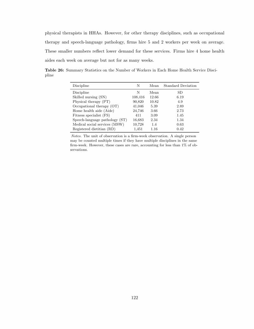
physical therapists in HHAs. However, for other therapy disciplines, such as occupational
therapy and speech-language pathology, firms hire 5 and 2 workers per week on average.
These smaller numbers reflect lower demand for these services. Firms hire 4 home health
aides each week on average but not for as many weeks.
Table 26: Summary Statistics on the Number of Workers in Each Home Health Service Disci-pline
Discipline N Mean Standard Deviation
Discipline N Mean SDSkilled nursing (SN) 108,416 12.66 6.19Physical therapy (PT) 90,820 10.82 4.9Occupational therapy (OT) 41,046 5.39 2.89Home health aide (Aide) 24,746 3.66 2.73Fitness specialist (FS) 411 3.09 1.45Speech-language pathology (ST) 16,683 2.34 1.34Medical social services (MSW) 10,728 1.4 0.63Registered dietitian (RD) 1,451 1.16 0.42
Notes. The unit of observation is a firm-week observation. A single personmay be counted multiple times if they have multiple disciplines in the samefirm-week. However, these cases are rare, accounting for less than 1% of ob-servations.
122

BIBLIOGRAPHY
K. G. Abraham and S. K. Taylor. Firms’ use of outside contractors: Theory and evidence.Journal of Labor Economics, XIV:394424, 1996.
L. H. Aiken, S. P. Clarke, D. M. Sloane, J. Sochalski, and J. H. Silber. Hospital nursestaffing and patient mortality, nurse burnout, and job dissatisfaction. Journal of theAmerican Medical Association, 288(16):1987–1993, 2002.
L. H. Aiken, Y. Xue, S. P. Clarke, and D. M. Sloane. Supplemental nurse staffing in hospitalsand quality of care. The Journal of Nursing Administration, 37(7-8):335, 2007.
L. H. Aiken, D. M. Sloane, J. P. Cimiotti, S. P. Clarke, L. Flynn, J. A. Seago, J. Spetz, andH. L. Smith. Implications of the california nurse staffing mandate for other states. HealthServices Research, 45(4):904–921, apr 2010. doi: 10.1111/j.1475-6773.2010.01114.x. URLhttp://dx.doi.org/10.1111/j.1475-6773.2010.01114.x.
L. H. Aiken, J. Shang, Y. Xue, and D. M. Sloane. Hospital use of agency-employed supple-mental nurses and patient mortality and failure to rescue. Health Services Research, 48(3):931–948, 2013.
S. G. Allen. How much does absenteeism cost? Journal of Human Resources, pages 379–393,1983.
D. Angrist Joshua and J.-S. Pischke. Mostly Harmless Econometrics: An Empiricists Com-panion. Princeton University, 2009.
S.-H. Bae, B. Mark, and B. Fried. Use of temporary nurses and nurse and patient safetyoutcomes in acute care hospital units. Health Care Management Review, 35(4):333–344,2010.
G. Baker, R. Gibbons, and K. J. Murphy. Relational contracts and the theory of the firm.Quarterly Journal of Economics, pages 39–84, 2002.
L. C. Baker, C. S. Phibbs, C. Guarino, D. Supina, and J. L. Reynolds. Within-year variationin hospital utilization and its implications for hospital costs. Journal of Health Economics,23:191–211, 2004. doi: 10.1016/j.jhealeco.2003.09.005.
A. V. Banerjee and E. Duflo. Reputation effects and the limits of contracting: A study ofthe indian software industry. Quarterly Journal of Economics, 115(3):989–1017, aug 2000.doi: 10.1162/003355300554962. URL http://dx.doi.org/10.1162/003355300554962.
R. N. Batra and A. Ullah. Competitive firm and the theory of input demand under priceuncertainty. Journal of Political Economy, 82(3):537–548, 1974.
J. A. Berry Jaeker and A. L. Tucker. Past the point of speeding up: The negative effects ofworkload saturation on efficiency and patient severity. Management Science, pages 1–21,2016.
123
A. L. Booth, M. Francesconi, and J. Frank. Temporary jobs: stepping stones or dead ends?The Economic Journal, 112(480):F189–F213, 2002.
T. Brachet, G. David, and A. M. Drechsler. The effect of shift structure on performance.American Economic Journal: Applied Economics, pages 219–246, 2012.
S. Braguinsky, A. Ohyama, T. Okazaki, and C. Syverson. Acquisitions, productivity, andprofitability: Evidence from the japanese cotton spinning industry. American EconomicReview, 105(7):2086–2119, jul 2015. doi: 10.1257/aer.20140150. URL http://dx.doi.
org/10.1257/aer.20140150.
J. P. Broschak and A. Davis-Blake. Mixing standard work and nonstandard deals: The con-sequences of heterogeneity in employment arrangements. The Academy of ManagementJournal, 49(2):371–393, 2006. ISSN 00014273. URL http://www.jstor.org/stable/
20159769.
C. Brown and J. L. Medoff. Firm age and wages. Journal of Labor Economics, 21(3):677–697, 2003.
J. Brown, M. Duggan, I. Kuziemko, and W. Woolston. How does risk selection respond torisk adjustment? new evidence from the medicare advantage program. The AmericanEconomic Review, 104(10):3335–3364, 2014.
Bureau of Labor Statistics. Absences from work of employed full-time wage and salaryworkers by occupation and industry. Website, 2017. URL https://www.bls.gov/cps/
cpsaat47.html.
W. Cabin, D. U. Himmelstein, M. L. Siman, and S. Woolhandler. For-profit medicare homehealth agencies’ costs appear higher and quality appears lower compared to nonprofitagencies. Health Affairs, 33(8):1460–1465, 2014.
H. L. Carmichael. Reputations in the labor market. The American Economic Review, 74(4):713–725, 1984. ISSN 00028282. URL http://www.jstor.org/stable/1805135.
A. Chandra, A. Finkelstein, A. Sacarny, and C. Syverson. Health care exceptionalism?performance and allocation in the us health care sector. American Economic Review, 106(8):2110–44, August 2016. doi: 10.1257/aer.20151080. URL http://www.aeaweb.org/
articles?id=10.1257/aer.20151080.
K. Chapple. Time to work: Job search strategies and commute time for women on welfarein san francisco. Journal of Urban Affairs, 23(2):155–173, 2001.
A. Cook, M. Gaynor, M. Stephens Jr, and L. Taylor. The effect of a hospital nurse staffingmandate on patient health outcomes: Evidence from california’s minimum staffing regu-lation. Journal of Health Economics, 31(2):340–348, 2012.
N. D. Cuyper, J. de Jong, H. D. Witte, K. Isaksson, T. Rigotti, and R. Schalk. Literaturereview of theory and research on the psychological impact of temporary employment:Towards a conceptual model. International Journal of Management Reviews, 10(1):25–51, mar 2008. doi: 10.1111/j.1468-2370.2007.00221.x. URL http://dx.doi.org/10.
1111/j.1468-2370.2007.00221.x.
124
G. David and T. Brachet. Retention, learning by doing, and performance in emergencymedical services. Health Services Research, 44(3):902–925, 2009.
G. David and K. Kim. The effect of workforce assignment on performance: Evidence fromhome health care. Working Paper, 2017.
G. David and D. Polsky. Home health services, economics of. In Encyclopedia of HealthEconomics, pages 477–483. Elsevier BV, 2014. doi: 10.1016/b978-0-12-375678-7.01003-8.URL http://dx.doi.org/10.1016/B978-0-12-375678-7.01003-8.
G. David, E. Rawley, and D. Polsky. Integration and task allocation: Evidence from patientcare. Journal of Economics and Management Strategy, 22(3):617–639, 2013.
A. K. Dixit and R. S. Pindyck. Investment Under Uncertainty. PrincetonUniversity Press, Princeton, New Jersey, 1994. ISBN 0691034109. URLhttp://www.ebook.de/de/product/3239261/avinash_k_dixit_robert_s_pindyck_
investment_under_uncertainty.html.
J. J. Doyle Jr, J. A. Graves, J. Gruber, and S. A. Kleiner. Measuring returns to hospitalcare: Evidence from ambulance referral patterns. Journal of Political Economy, 123(1):170–214, 2015.
T. Dunne, M. J. Roberts, and L. Samuelson. The growth and failure of us manufacturingplants. The Quarterly Journal of Economics, 104(4):671–698, 1989.
R. G. Ehrenberg. Absenteeism and the overtime decision. The American Economic Review,60(3):352–357, 1970.
Federal Register. Medicare program; home health prospective payment system rate updatefor calendar year 2015; final rule. 79(215):66032–, November 2014.
W. E. Ferson. Investment performance: A review and synthesis. In Handbook of the Eco-nomics of Finance, pages 969–1010. Elsevier BV, 2013. doi: 10.1016/b978-0-44-459406-8.00014-7. URL http://dx.doi.org/10.1016/B978-0-44-459406-8.00014-7.
D. N. Figlio, M. O. Schapiro, and K. B. Soter. Are tenure track professors better teachers?Review of Economics and Statistics, 97(4):715–724, oct 2015. doi: 10.1162/rest a 00529.URL http://dx.doi.org/10.1162/REST_a_00529.
D. Foote and T. Folta. Temporary workers as real options. Human Resource ManagementReview, 12:579–97, 2002.
B. Friedman and M. V. Pauly. Cost functions for a service firms with variable quality andstochastic demand: the case of hospitals. Review of Economics and Statistics, 63(4):620–624, 1981.
L. Garicano and T. Santos. Referrals. The American Economic Review, 94(3):499–525,2004.
M. Gaynor, K. Ho, and R. Town. The industrial organization of health care markets.Technical report, National Bureau of Economic Research, 2014.
125
J. I. Gimenez-Nadal, J. A. Molina, et al. Commuting time and labour supply: A causaleffect? IZA Discussion Paper, (5529), Feb. 2011.
L. V. Green, S. Savin, and N. Savva. nursevendor problem: Personnel staffing in the presenceof endogenous absenteeism. Management Science, 59(10):2237–2256, 2013.
L. Guiso and G. Parigi. Investment and demand uncertainty. The Quarterly Journal ofEconomics, 114(1):185–227, 1999.
J. Guo, R. T. Konetzka, and W. G. Manning. The causal effects of home care use oninstitutional long-term care utilization and expenditures. Health Economics, 24(S1):4–17, 2015.
A. Gupta. Impacts of performance pay for hospitals: The readmissions reduction program.Technical report, Working Paper, 2016.
E. Gutierrez-i Puigarnau and J. N. van Ommeren. Labour supply and commuting. Journalof Urban Economics, 68(1):82–89, 2010.
J. C. Haltiwanger, J. I. Lane, and J. R. Spletzer. Productivity differences across employers:The roles of employer size, age, and human capital. American Economic Review, 89(2):94–98, may 1999. doi: 10.1257/aer.89.2.94. URL http://dx.doi.org/10.1257/aer.89.
2.94.
D. S. Hamermesh and G. A. Pfann. Adjustment costs in factor demand. Journal of Eco-nomic Literature, 34(3):1264–1292, 1996.
B. Harley. The conditions associated with peripheral employment in Australia. EmployeeRelations, 16(8):19–31, dec 1994. doi: 10.1108/01425459410073924. URL http://dx.
doi.org/10.1108/01425459410073924.
R. Hartman. Factor demand with output price uncertainty. The American EconomicReview, 66(4):675–681, 1976.
J. M. Hockenberry and E. R. Becker. How do hospital nurse staffing strategies affect patientsatisfaction? ILR Review, pages 890–910, 2016.
R. S. Huckman and G. P. Pisano. The firm specificity of individual performance: Evidencefrom cardiac surgery. Management Science, 52(4):473–488, apr 2006. doi: 10.1287/mnsc.1050.0464. URL http://dx.doi.org/10.1287/mnsc.1050.0464.
S. F. Jencks, M. V. Williams, and E. A. Coleman. Rehospitalizations among patients in themedicare fee-for-service program. New England Journal of Medicine, 360(14):1418–1428,2009.
G. Z. Jin and P. Leslie. Reputational incentives for restaurant hygiene. American EconomicJournal: Microeconomics, 1(1):237–267, 2009.
E. M. Johnson. Ability, learning and the career path of cardiac specialists. Cambridge,Massachusetts Institute of Technology, 2011.
126

L. F. Katz and A. B. Krueger. The rise and nature of alternative work arrangements in theunited states, 1995-2015. National Bureau of Economic Research, Working Paper(22667),09 2016.
I. Kawachi, N. Daniels, and D. E. Robinson. Health disparities by race and class: why bothmatter. Health Affairs, 24(2):343–352, 2005.
H. Kim and E. C. Norton. Practice patterns among entrants and incumbents in the homehealth market after the prospective payment system was implemented. Health Economics,24(S1):118–131, 2015.
S.-H. Kim, C. W. Chan, M. Olivares, and G. Escobar. ICU admission control: An em-pirical study of capacity allocation and its implication for patient outcomes. Man-agement Science, 61(1):19–38, jan 2015. doi: 10.1287/mnsc.2014.2057. URL http:
//dx.doi.org/10.1287/mnsc.2014.2057.
B. Klein and K. B. Leffler. The role of market forces in assuring contractual performance.The Journal of Political Economy, pages 615–641, 1981.
L. J. Kozak, M. J. Hall, and M. F. Owings. Trends in avoidable hospitalizations, 1980–1998.Health Affairs, 20(2):225–232, 2001.
L. Kuntz, R. Mennicken, and S. Scholtes. Stress on the ward: Evidence of safety tippingpoints in hospitals. Management Science, 61(4):754–771, 2014.
C. Laine, L. Goldman, J. R. Soukup, and J. G. Hayes. The impact of a regulation restrictingmedical house staff working hours on the quality of patient care. Journal of the AmericanMedical Association, 269(3):374–378, 1993.
K. B. Lasater, D. M. Sloane, and L. H. Aiken. Hospital employment of supplementalregistered nurses and patients’ satisfaction with care. The Journal of Nursing Ad-ministration, 45(3):145–151, mar 2015. doi: 10.1097/nna.0000000000000174. URLhttp://dx.doi.org/10.1097/NNA.0000000000000174.
J. Levin. Multilateral contracting and the employment relationship. Quarterly Journal ofEconomics, pages 1075–1103, 2002.
H. Lin. Revisiting the relationship between nurse staffing and quality of care in nursinghomes: An instrumental variables approach. Journal of Health Economics, 37:13–24,2014.
F. Lotti and E. Viviano. Temporary workers, uncertainty and productivity. The Society ofLabor Economists, mimeo, 2012.
S. F. Lu and L. X. Lu. Do mandatory overtime laws improve quality? staffing decisionsand operational flexibility of nursing homes. Management Science, aug 2016.
R. Macchiavello and A. Morjaria. The value of relationships: Evidence from a supply shockto kenyan rose exports. The American Economic Review, 105(9):2911–2945, sep 2015.doi: 10.1257/aer.20120141. URL http://dx.doi.org/10.1257/aer.20120141.
127

M. A. Makary and M. Daniel. Medical error—the third leading cause of death in the u.s.BMJ, 353:i2139, 2016.
A. Manning. Monopsony in motion: Imperfect competition in labor markets. PrincetonUniversity Press, 2003.
B. A. Mark, D. W. Harless, J. Spetz, K. L. Reiter, and G. H. Pink. California’s minimumnurse staffing legislation: Results from a natural experiment. Health Services Research,48(2pt1):435–454, 2013. ISSN 1475-6773. doi: 10.1111/j.1475-6773.2012.01465.x. URLhttp://dx.doi.org/10.1111/j.1475-6773.2012.01465.x.
A. Mas and E. Moretti. Peers at work. The American Economic Review, 99(1):112–145,2009.
J. D. Matsudaira. Government regulation and the quality of healthcare evidence fromminimum staffing legislation for nursing homes. Journal of Human resources, 49(1):32–72, 2014.
J. McMillan and C. Woodruff. Interfirm relationships and informal credit in Vietnam.The Quarterly Journal of Economics, 114(4):1285–1320, nov 1999. doi: 10.1162/003355399556278. URL http://dx.doi.org/10.1162/003355399556278.
J. L. Medoff and K. G. Abraham. Experience, performance, and earnings. The QuarterlyJournal of Economics, 95(4):703–736, 1980.
MedPAC. Report to the Congress: Medicare Payment Policy, chapter Home HealthCare Services, pages 213–238. March 2014. URL http://www.medpac.gov/docs/
default-source/reports/mar14_ch09.pdf?sfvrsn=0.
MedPAC. Report to the Congress: Medicare Payment Policy, chapter Home Health CareServices, pages 209–234. March 2016a. URL http://www.medpac.gov/documents/
reports/chapter-9-home-health-care-servichttp://www.medpac.gov/documents/
reports/chapter-8-home-health-care-services-(march-2016-report).pdf?
sfvrsn=0.
MedPAC. Data Book: Healthcare Spending and the MedicareProgram, volume 116. Washington: MedPAC, June, 2016b.URL http://www.medpac.gov/docs/default-source/data-book/
june-2016-data-book-health-care-spending-and-the-medicare-program.pdf?
sfvrsn=0.
R. J. Murnane and B. R. Phillips. Learning by doing, vintage, and selection: Three piecesof the puzzle relating teaching experience and teaching performance. Economics of Edu-cation Review, 1(4):453–465, 1981.
M. I. Nadiri and S. Rosen. A Disequilibrium Model of Demand for Factors of Production.National Bureau of Economic Research, New York, 1973.
A. Navathe and G. David. The formation of peer reputation among physicians and itseffect on technology adoption. Journal of Human Capital, 3(4):289–322, dec 2009. doi:10.1086/652900. URL http://dx.doi.org/10.1086/652900.
128
M. D. Naylor, D. Brooten, R. Campbell, B. S. Jacobsen, M. D. Mezey, M. V. Pauly, andJ. S. Schwartz. Comprehensive discharge planning and home follow-up of hospitalizedelders: A randomized clinical trial. Journal of the American Medical Association, 281(7):613–620, 1999.
M. D. Naylor, E. T. Kurtzman, D. C. Grabowski, C. Harrington, M. McClellan, and S. C.Reinhard. Unintended consequences of steps to cut readmissions and reform paymentmay threaten care of vulnerable older adults. Health Affairs, pages 10–1377, 2012.
J. Needleman, P. Buerhaus, V. S. Pankratz, C. L. Leibson, S. R. Stevens, and M. Harris.Nurse staffing and inpatient hospital mortality. New England Journal of Medicine, 364(11):1037–1045, 2011.
W. Y. Oi. The desirability of price instability under perfect competition. Econometrica:Journal of the Econometric Society, pages 58–64, 1961.
W. Y. Oi and T. L. Idson. Firm size and wages. Handbook of Labor Economics, 3:2165–2214,1999.
L. A. Petersen, T. A. Brennan, A. C. O’Neil, E. F. Cook, and T. H. Lee. Does housestaffdiscontinuity of care increase the risk for preventable adverse events? Annals of InternalMedicine, 121(11):866–872, 1994.
J. C. Pham, M. Andrawis, A. D. Shore, M. Fahey, L. Morlock, and P. J. Pronovost. Aretemporary staff associated with more severe emergency department medication errors?Journal for Healthcare Quality, 33(4):9–18, 2011.
D. Polsky, G. David, J. Yang, B. Kinosian, and R. M. Werner. The effect of entry regulationin the health care sector: The case of home health. Journal of Public Economics, 110:1–14, 2014.
Pricewaterhouse Coopers’ Health Research Institute. The price of excess: Identifying wastein healthcare spending, 2008. URL http://www.oss.net/dynamaster/file_archive/
080509/59f26a38c114f2295757bb6be522128a/The%20Price%20of%20Excess%20-%
20Identifying%20Waste%20in%20Healthcare%20Spending%20-%20PWC.pdf.
M. Raddish, S. D. Horn, and P. D. Sharkey. Continuity of care: Is it cost effective? AmericanJournal of Managed Care, 5(6):727–34, 1999.
J. B. Rebitzer and L. J. Taylor. A model of dual labor markets when product demand isuncertain. The Quarterly Journal of Economics, 106(4):1373–1383, 1991.
W. C. Richardson, D. M. Berwick, J. Bisgard, L. Bristow, C. Buck, C. Cassel, et al. Crossingthe quality chasm: A new health system for the 21st century, 2001.
L. A. Riesenberg, J. Leitzsch, J. L. Massucci, J. Jaeger, J. C. Rosenfeld, C. Patow, J. S. Pad-more, and K. P. Karpovich. Residents’ and attending physicians’ handoffs: A systematicreview of the literature. Academic Medicine, 84(12):1775–1787, 2009.
129
D. Russell, R. J. Rosati, P. Rosenfeld, and J. M. Marren. Continuity in home health care:Is consistency in nursing personnel associated with better patient outcomes? Journal forHealthcare Quality, 33(6):33–39, 2011.
A. Sandmo. On the theory of the competitive firm under price uncertainty. The AmericanEconomic Review, 61(1):65–73, 1971.
J. W. Saultz and J. Lochner. Interpersonal continuity of care and care outcomes: A criticalreview. The Annals of Family Medicine, 3(2):159–166, 2005.
N. Sood, P. J. Huckfeldt, J. J. Escarce, D. C. Grabowski, and J. P. Newhouse. Medicaresbundled payment pilot for acute and postacute care: analysis and recommendations onwhere to begin. Health Affairs, 30(9):1708–1717, 2011.
F. Tavares-Pereira, J. R. Figueira, V. Mousseau, and B. Roy. Multiple criteria dis-tricting problems. Annals of Operations Research, 154(1):69–92, may 2007. doi:10.1007/s10479-007-0181-5. URL http://dx.doi.org/10.1007/s10479-007-0181-5.
P. K. Tong. The effects of california minimum nurse staffing laws on nurse labor and patientmortality in skilled nursing facilities. Health Economics, 20(7):802–816, 2011. ISSN 1099-1050. doi: 10.1002/hec.1638. URL http://dx.doi.org/10.1002/hec.1638.
J. H. Wasson, A. E. Sauvigne, R. P. Mogielnicki, W. G. Frey, C. H. Sox, C. Gaudette, andA. Rockwell. Continuity of outpatient medical care in elderly men: A randomized trial.Journal of the American Medical Association, 252(17):2413–2417, 1984.
H. D. Witte and K. Nswall. ‘objective’ vs ‘subjective’ job insecurity: Consequences oftemporary work for job satisfaction and organizational commitment in four europeancountries. Economic and Industrial Democracy, 24(2):149–188, may 2003. doi: 10.1177/0143831x03024002002. URL http://dx.doi.org/10.1177/0143831X03024002002.
C. A. Woodward, J. Abelson, S. Tedford, and B. Hutchison. What is important to continuityin home care?: Perspectives of key stakeholders. Social Science and Medicine, 58(1):177–192, 2004.
T. Worth. Home health on road to reducing readmits. Healthcare Fi-nance, April 07 2014. URL http://www.healthcarefinancenews.com/news/
home-health-road-reducing-readmits. April 7, 2014 (Accessed on July 8, 2016).
Y. Xue, L. H. Aiken, D. A. Freund, and K. Noyes. Quality outcomes of hospital supplementalnurse staffing. Journal of Nursing Administration, 42(12):580–585, 2012.
130