The Design of DAQ Circuit Board Processor Cooling Methods

The Design of DAQ Circuit Board Processor Cooling Methods in an Aluminum Enclosure

Submitted to:

Paulina Mosely, Project Engineer National Instruments

Austin, Texas

ME466K Mechanical Engineering Design Projects Professor Steven P. Nichols

Summer 1999

Prepared by:

Steve C. Talbot, Team Leader Raul Rodriguez

Chris Specht

2

Executive Summary

National Instruments is a major supplier of data acquisition (DAQ) equipment in

the measurement and testing industry. N.I. has had trouble managing excess heat

produced by components on the circuit boards in these DAQ units. National Instruments

has requested that the design team survey microprocessor industry cooling methods. The

design team researched heat sinks, forced convective air flow via small electronic fans,

thermal electric coolers, heat pipes, chip electronic refrigeration equipment, liquid

immersion coolants, and heat exchangers (see section V, “Solution Refinement”).

However, after the team considered cost (see section IV, “Project Cost Analysis”),

availability, feasibility, and compared each device’s performance parameters to the

team’s design constraints (see section V, “Solution Refinement), the team chose to test

heat sinks, heat pipes, and electric fans, separately and in combination. The design team

built a prototype of an aluminum DAQ enclosure and formulated a plan for testing the

cooling method alternative. N.I. provided the design group with Virtual Bench for

LabVIEW temperature measurement software and thermocouple wires to aid the group in

its experimentation and selection of alternative methods. The team recorded temperature

data with the measurement software and analyzed the data for trends that indicated

advantageous properties inherent to particular cooling methods.

For comparison purposes, the team compiled a table of temperature values taken

during experimentation for each cooling variant (See tables 3 and 4 in section VI,

“Experimentation”). These tables listed the steady state temperature readings reached for

3

each experiment with and without the aid of a fan. From these values, the team

calculated the junction temperatures of a typical DAQ microprocessor (see tables 5,6, and

7 in section VI, “Experimentation”). The team plotted the data from these tables, and

derived an equation that allowed them to give National Instruments the ability to estimate

the temperature of the junction temperature attainable at any wattage. Based upon this

relation, the team calculated that for the heat pipe with aluminum mounting plate and

pinned heat sink that utilized only natural convection, the junction temperature of a chip

would be able to remain at or below 110 °C for power levels up to approximately 7.75

watts in an ambient temperature of 55 °C. Utilizing the heat pipe setup with

impingement fan, the junction temperature could remain at or below 110 °C for power

levels up to approximately 13.75 watts in an ambient temperature of 55 °C (see section

6.2.6 “Description and Analysis of Variants Tested”).

By noting the cooling capabilities of the various scenarios, the team became

aware that some of the cooling methods would be applicable at different wattages. For

the lower wattages, a spreader or heat sink could be used if necessary. For the middle

wattage values, a heat pipe utilizing only natural convection could be utilized. Finally,

for the upper values including the 16 watt dissipation used in the initial testing

(corresponding to 10 watts from the main mock chip) a heat pipe with impingement flow

could effectively cool the chip.

4

I. Introduction

National Instruments is a major supplier of data acquisition (DAQ) equipment in

the measurement and testing industry. N.I. has had trouble managing excess heat

produced by components on the circuit boards in their DAQ units. As the heat builds, it

reduces the efficiency and speed of the circuitry, and may even damage the circuit board

components. Ever searching for innovative solutions to challenging design problems,

N.I. has sponsored a design team from the University of Texas at Austin to analyze the

DAQ heat problem. The team, consisting of members Raul Rodriguez, Chris Specht, and

Steve Talbot, refer to this problem as the “Cool Box” project.

1.1 Company Background

National Instruments (N.I.) was formed in 1976 by Dr. James Truchard and two

colleagues from the University of Texas at Austin [“Vision and Culture,” 1999].

Focusing on innovation, growth, and leadership, N.I. began production on its first

General-Purpose Interface Bus for connecting standard desktop PCs to traditional

measurement instruments in 1977 [“Our History,” 1999]. N.I. continued development of

PC-based measurement and automation hardware throughout the next decade and a half,

releasing instrumentation software, industrial automation hardware and software, general-

purpose machine vision systems, and data acquisition hardware and software for analysis

of physical data, among other products (Figure 1) [“What We Make and Sell,” 1999].

5

Earning approximately $40 million dollars net profit annually [“National Instruments…

Growth In First Quarter,” 1999], National Instruments services the telecommunication,

automotive, semiconductor, aerospace, electronics, chemical, and pharmaceutical

industries from its 37 offices in 27 countries throughout Europe, Asia, and North and

Latin America [“Worldwide Offices,” 1999].

1.2 Product Background

National Instruments designed its first data acquisition boards (DAQ) in 1987 for

analyzing physical data such as temperature, pressure, or vibration. N.I. designed the

DAQ boards to function as the hardware interface between physical measurement

instrument sensors and personal computers running N.I.’s LabVIEW virtual

Figure 1 : Company (CW from upper left) I/O Distributor, Vision System, I/O board, DAQPad, LavView [National Instruments catalog, 1999].

6

instrumentation software package. When monitoring temperature for example,

thermocouples are attached to the DAQ, which in turn are attached to the CPU where

incoming data could be recorded and analyzed by LabView. Other instrumentation

manufacturers have designed costly fixed-function, self-contained DAQ and analysis

software combination systems. N.I. is seeking to compete with these other manufacturers

by addressing the disadvantages of self-contained systems, relying on the attractiveness

and power they could obtain from PCs. Today, National Instruments is one of the

world’s leading DAQ hardware suppliers. [“Our History,” 1999].

Traditionally, most data acquisition boards have been comprised of a circuit board

with input and output ports attached. These DAQ’s are then inserted into a CPU. Having

to insert the DAQ board every time into the CPU can often be undesirable or

inconvenient to the customer. For this reason, N.I. began designing DAQ’s that were

self-contained, while still adhering to a philosophy of keeping their DAQ hardware and

analysis software separate. In other words, each DAQ was manufactured with its own

enclosure and ports.

II. Project Background

The DAQPad-6070E is a data acquisition unit designed to route analog and digital

instrumentation signals via a physical cable connection to a PC for analysis. The

DAQPad-6070E consists of a metal enclosure housing several circuit boards, RF

connections, and power input/output connections (Figure 2). The circuit boards and their

components can heat up due to internal resistances inherent to all circuitry. The majority

7

of this heat is dissipated from the main processor chip. Heat sources nearby the DAQ

also contribute heat energy to the system (Figure 3).

Currently N.I. regulates the total amount of heat energy that the circuit boards are

subjected to during operation by including a small fan in the DAQ enclosure that actively

Figure 3. Typical DAQ Orientation [National Instru ments catalog, 1999].

Figure 2: DAQPad-6020E [National Instruments catalog, 1999].

8

provides forced convective airflow. However, N.I. wished to decrease the width of the

current DAQ enclosure by two-thirds, requiring the team to analyze the current heat

management strategy of the enclosed circuit board. Also, N.I. wanted the team to survey

the current cooling technology available to devise an efficient method for cooling the

enclosure that meets the constraints and requirements for the smaller product.

2.1 Constraints

Currently the DAQ enclosure has dimensions 12.1 inches wide, 10 inches deep,

and 1.7 inches high (Figure 4). This height is the measurement and testing industry

standard for DAQ equipment and was a constraint on the enclosure redesign. The DAQ

enclosure can be positioned for use in any of three orientations. The DAQ equipment is

often rack mounted either horizontally or vertically in its first two positions. The

industry standard length between rack slots is 1.7 inches. Therefore two of the

dimensions of the enclosure, height and width, should be some multiple of this 1.7 inch

industry standard length to accommodate the horizontal and vertical positions.

Figure 4: Current DAQ Dimensions [National Instruments catalog, 1999].

9

In addition, the width of the enclosure design could not be any smaller than the

circuit boards that it will enclose (Figure 5). The DAQ equipment is also often

positioned next to a laptop computer (Figure 3). This third orientation for the DAQ is the

most difficult to design because the end user will likely position the DAQ on its side,

backwards, or even upside down, introducing further position considerations. Finally, the

cost and availability of materials used for the enclosure were also constraints for this

project.

2.2 Requirements

The most important requirement for this project was that the team equip the

enclosure with a cooling method that would significantly reduce the chip junction and

circuitry temperatures. A junction temperature that the team aimed for was 110°C, as

suggest by their sponsor. This value is a typical junction temperature that might be

specified by chip manufacturers for optimal chip performance. This cooling technique

Figure 5: Circuit board to be cooled (5.3 in X 7.7 in)

10

needed to cost less than $50 dollars per box over the current design, be able to operate in

various orientations (e.g. on its side), have no vents on the top or sides of the enclosure,

and dissipate approximately 25 Watts. Additionally, the enclosure width needed to be

smaller than the current size, but no smaller than one-third its current size. Finally, using

computational fluid dynamic software or proper experimentation needed to be done

before prototypes were built.

III. Methodology

The approach the team used for this project was a hybrid of methodologies

containing elements of redesign, selection design, configuration design, and parametric

design. The team considered several factors when tailoring their version (Figure 6).

Problem Introduction

Determine Specifications

Alternative Solutions

Solution Refinement

Testing

Evaluations

Final Decision

Flow/H.T. Models

Design Box

Order Parts

Research

Figure 6. Methodology Flowchart

11

Among these factors were the time constraint and the absence of a customer driven

analysis.

Our methodology first required that the team clarify an original problem

statement, and then develop a specification sheet detailing the constraints and

requirements of their project (appendix A). The team then begins to evaluate the possible

solutions available as well as exploring new and inventive solutions. Before the first

phase of solution refinement can begin, the team creates mass flow and heat transfer

models and compares each. These models would give the team an understanding of how

typical cooling setups might work (e.g. a fan over a flat plate, or a heat sink). The team

refines the solution by using the specification sheet to compare the design parameters

against the criteria. After ordering the parts needed for experimentation, the team makes

a test enclosure to simulate the enclosure of the final product. The team then carries out

testing using the cooling components and test enclosure with varying arrangements and

conditions. The size of the test enclosure may vary from one possible solution to the

next. After testing the selected cooling solutions, the team evaluates the test results,

culminating in a final decision and a useful cooling method. Throughout the team’s

design process, this procedure allowed for late changes that might result from research of

new cooling methods not yet tested by the team.

12

IV. Project Cost Analysis

4.1 Professional Consultation and Services

The team instigated a rigorous cost analysis of the “Cool Box” project. The team

first analyzed the contribution to their project by outside consultants. The team’s

corporate sponsor, Paulina Mosley, loaned the team a set of thermocouples for sensing

temperatures on the DAQ circuit board and a N.I. thermal analysis software package

called Virtual Bench for LabVIEW. Paulina did not require the team to pay for the use of

this equipment. Doctor Raul G. Longoria of the Mechanical Engineering department of

the University of Texas at Austin offered the team the supervised use of the computers

and electronic equipment in his electronics lab. Doctor Longoria did not require payment

for this usage. Doctor Dennis E. Wilson and Doctor Ofodike A. Ezekoye of the

University of Texas both advised the team on current computer processor cooling

methods based upon the doctors’ many years of engineering experience. These

professors required no consultation fee for their services.

4.2 Price Data

The team checked web sites, magazines, and vendor catalogs of heat sinks,

cooling fans, heat pipes, and thermal greases. The team was able to set ranges of costs of

these products based upon information available on the internet. These costs were

compiled and can be seen in table 1 below. In the first column of table 1, the current

cooling products available for purchase are listed, with the most affordable product types

13

listed in bold characters. Also noted in the table are the web pages from which the team

found these price ranges.

Table 1: Product Price Ranges

Product Type Price/Item Range Source of Data

Heat Sink $0.69 - $2.00 www.chipcoolers.com Heat Pipe $5.00 - $10.00 www.thermacore.com

Impinging Fan $4.00 - $15.00 www.coolinnovations.com Centrifugal Fan $1.00-$4.00 www.coolinnovations.com

Sleeve Bearing Fan $1.00-$4.00 www.indek.com Ball Bearing Fan $4.00-$8.00 www.aptekus.com

Thermal Electric Cooler (TEC) $40.00 - $50.00 www.aoc-cooler.com Thermal Grease/Adhesive $1.99 - $10.00 www.aptekus.com

Based upon these ranges of prices for cooling products, the team calculated the

approximate cost of testing different cooling methods. The cooling methods listed in

table 2 below are feasible combinations of the previously listed product types from table

1 above that the team felt were feasible for testing. The approximate cost ranges listed in

the second column of table 2 were calculated by summing the” Price/Item” of each

“Product Type” for a “Cooling Method” for both the lower and upper bounds of the cost

range. The “Order of Least Expense” column of table 2 rates the cooling methods from

the least (1) to most (16) expensive method.

14

Table 2: Product Combinations

Cooling Methods Approximate Cost Range Order of Least Expense Heat Sink $0.69 - $2.00 1 Ball Bearing Fan $5.00 - $10.00 10 Sleeve Bearing Fan $1.00-$4.00 2 Impinging Fan $4.00 - $15.00 7 Heat Sink and Ball Bearing Fan $4.69 - $10.00 8 Heat Sink and Sleeve Bearing Fan $1.69 - $6.00 3 Heat Sink and Impinging Fan $4.69 - $17.00 9 Heat Sink and Centrifugal Fan $1.69 - $6.00 4 Heat Sink, Ball Bearing Fan, and Thermal Grease $6.68 - $20.00 11 Heat Sink, Sleeve Bearing Fan, and Thermal Grease $3.68 - $16.00 5 Heat Sink, Impinging Fan, and Thermal Grease $6.68 - $27.00 12 Heat Sink, Centrifugal Fan, and Thermal Grease $3.68 - $16.00 6 Heat Sink, Ball Bearing Fan, Thermal Grease, and TEC $46.68 - $70.00 15 Heat Sink, Sleeve Bearing Fan, Thermal Grease, and TEC $43.68 - $66.00 13 Heat Sink, Impinging Fan, Thermal Grease, and TEC $46.68 - $77.00 16 Heat Sink, Centrifugal Fan, Thermal Grease, and TEC $43.68 - $66.00 14

4.3 Cost Strategy

The team’s strategy for testing was to begin using a single product type as their

cooling method, measuring temperature data, and continuing to add appropriate product

types to their cooling method in a manner similar to the cooling method listing of table 2.

Once the team identified a few optimized designs, they would discard the unused product

types in favor of a few chosen cooling methods that the team selects. Further details of

testing and prototype construction procedures that the team chose are discussed later in

this report. However, the team decided on some of these testing and prototype

construction procedures early on in the project, because they needed to analyze which

combinations added to the final prototype would be financially acceptable to their

sponsor National Instruments.

Adding product types increases the end cost of building test prototypes. The team

desired to keep the end cost of the final prototype and its production low, preferably

15

under $50 dollars. The team anticipated that the preferred product type or some

combination of product types used in the final prototype would be the heat sink, heat

pipe, impinging fan, ball bearing fan, centrifugal fan and/or thermal grease. A heat sink

was the least expensive product type, and could therefore be included in any cooling

method chosen. The thermal grease only adds about $2 dollars to the end cost of the

prototype. Thermal grease can be used with several cooling methods to reduce contact

resistance between surfaces. Because of the low cost of the thermal grease, the team

anticipated its use. The other product types listed all met the team’s $50 dollar upper

limit constraint, even in combination, except when the team included the more expensive

versions of thermal electric coolers (TECs) included in the cooling method. These TECs

have a retail price of $49.95, and are custom made for each customer application.

However, the team anticipated a reduction in cost for the TEC if purchased in bulk which

would make the most expensive versions affordable. If used the team would choose the

lowest priced versions to first prove the TEC’s usefulness. If the TEC proved useful or

an inexpensive solution not found, the team would again consider more expensive TEC

versions with their anticipated cost reduction.

Paulina Mosley explained to the team that N.I. has a highly diverse selection of

products for sale, but that demand for each of their product lines is usually small. N.I.

can expect to produce five hundred to one thousand units in the first year of manufacture

and as many as five thousand in the subsequent years of manufacture for any of its

products. Manufacturers usually sell product types at reduced bulk rates in lots starting at

one thousand units. Local distributors sell lots of smaller sizes at retail prices [Jim

Palmisciano of ChipCoolers, 1999]. However, the team has calculated from the tables

16

above that when N.I. begins mass production of the DAQPad-6070E product type,

manufacturers will charge N.I. less than $50 dollars for the cooling methods used in the

DAQ, thus meeting the team’s end cost goal.

V. Solution Refinement

5.1 Alternate Design: Heat Sink

The first logical method for the cooling of circuitry that the team

examined was the application of heat sinks. Heat sinks are metal surfaces mounted to

components of a circuit board in order to increase component heat dissipation capacity.

Dissipated heat is convectively transported to a cross flow airstream or convectively

drawn away by inpinging airflow. Heat sinks increase the surface area of circuit board

components. These sinks are composed of several fins, pins, disks, or arms. Due to both

Fourier’s Heat Equation for both natural and forced convection and Newton’s Law of

Conduction, increased surface area increases heat dissipation from circuit board

components (figure 7).

TAhqconv

∆=

X

TKAq

cond ∆∆=

)(a

)(b

Figure 7: (a) Fourier’s Heat Equation (convection), (b) Newton’s Law of Cooling (conduction)

17

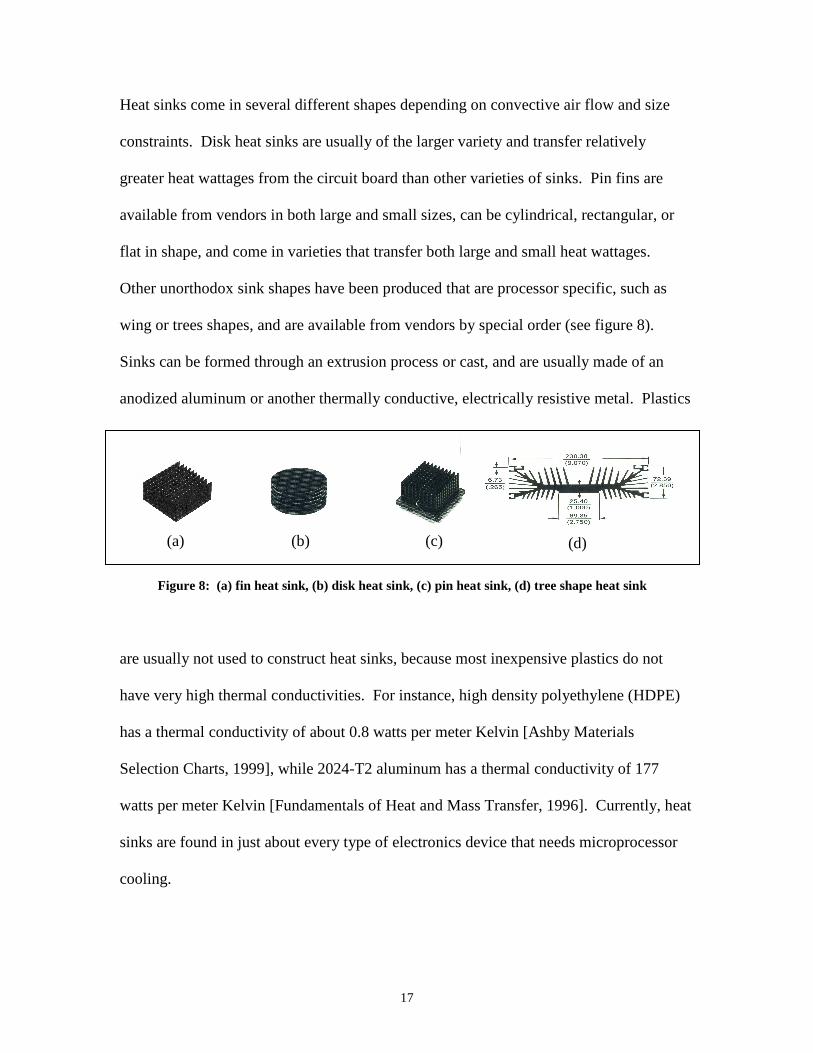
Heat sinks come in several different shapes depending on convective air flow and size

constraints. Disk heat sinks are usually of the larger variety and transfer relatively

greater heat wattages from the circuit board than other varieties of sinks. Pin fins are

available from vendors in both large and small sizes, can be cylindrical, rectangular, or

flat in shape, and come in varieties that transfer both large and small heat wattages.

Other unorthodox sink shapes have been produced that are processor specific, such as

wing or trees shapes, and are available from vendors by special order (see figure 8).

Sinks can be formed through an extrusion process or cast, and are usually made of an

anodized aluminum or another thermally conductive, electrically resistive metal. Plastics

are usually not used to construct heat sinks, because most inexpensive plastics do not

have very high thermal conductivities. For instance, high density polyethylene (HDPE)

has a thermal conductivity of about 0.8 watts per meter Kelvin [Ashby Materials

Selection Charts, 1999], while 2024-T2 aluminum has a thermal conductivity of 177

watts per meter Kelvin [Fundamentals of Heat and Mass Transfer, 1996]. Currently, heat

sinks are found in just about every type of electronics device that needs microprocessor

cooling.

Figure 8: (a) fin heat sink, (b) disk heat sink, (c) pin heat sink, (d) tree shape heat sink

(a) (b) (c) (d)

18

5.1.1 Good and Bad Features

Heat sinks are very inexpensive to produce and are the first logical step in

choosing cooling solutions. Heat sinks come in a wide variety of sizes. Heights and

lengths can range from a few millimeters to several centimeters. Because of this, almost

any chip type can have a mounted heat sink. Heat sinks are passive devices. Passive

devices operate without the input of power or electrical current, as compared to active

coolers that can use from .5 watts up to about 3 watts. They can be purchased in bulk

quantities of 100 or more for around $2.00 dollars each. They can be used with any of

the other cooling solutions presented herein, and they enhance the radiative and natural

convection mechanisms of dissipative heat transport for the board circuitry when those

are utilized. Tooling costs are low for heat sink assembly, as they require only one

additional step in a process for assembly. Component sinks come in a wide variety of

sizes, typically ranging from a 0.5 in2 surface area and 0.125 inch height, to a 3 in2

surface area and a 3 inch height. Unless they are exposed to corrosive environments,

such as that caused by condensation of water vapor through the use of TECs, they have

an unlimited life expectancy. Heat sinks can far outlast the 7 to 10 year life expectancy

of the DAQ device and could conceivably be reused.

Although heat sinks are available in small sizes, in order to achieve significant

heat transfer rates from circuitry components, large and bulky heat sinks are required.

Because of the limited space available in the DAQPad6070E between circuit boards, heat

sink size is a major issue. For the 0.5 inch spacing between circuit boards used by NI, the

team’s initial calculations reveal that even when used in conjunction with forced

convection, heat sinks small enough to be used in the team’s device enclosure do not

19

dissipate significant heat. These calculations stated that the chip’s temperature would be

reduced very little from an initial hypothetical temperature of 150oC to the team’s target

temperature of 110oC. Because the present cooling scheme for the DAQ6070E does

nothing more than recirculate hot air within its enclosure, and still reduces a hot chip at

150 oC to about 137 oC, and because of the simplicity and affordability of heat sinks, the

team felt that further heat sink investigations were warranted.

5.1.2 Preliminary Calculations

Since heat sinks have several different features effecting heat transfer, it is

difficult to calculate heat flux values accurately, but general values can be estimated. For

the case of the basic heat sink and the heat sink with cross flow it is sufficient to solve for

the sink-to-air resistance. This is because most manufacturers of heat sinks have

extensive empirical data that informs the buyer what resistance levels are possible for any

given heat sink. This information is usually communicated in graphical form with the

resistance as a function of the airflow for forced convection and change in temperature as

a function of wattage for natural convection. The sink-to-air resistance can be calculated

as follows:

where θsa, θ jc, andθ cs are the sink-to-air, junction-to-chip surface, and surface-to-sink

resistances, respectively. For our calculations, our group used a junction-to-chip surface

resistance of 2°C/W. This was a conservative estimate, and for most chips would not be

this high. The surface-to-sink resistance could be calculated for various interface

),( csjcj

sa Q

TTθθθ −−

−= ∞

20

compounds. When the sink-to-air resistance is solved for, it can be compared to graphs

provided by the sink manufacturers for any given sink. For forced convection, the buyer

could look up the required velocity to achieve the calculated resistance.

Using the above-described equation, several heat-to-sink resistances were

calculated for various wattages and chip sizes. The results are shown in appendix C.

Also included is a graphical representation of the required resistance as a function of chip

wattages for a chip the size of a Minimite chip (.95X.95 inches).

5.2 Alternate Design: Fan Crossflow

The first cooling method alternative for the compact version of the

DAQPad6070E that the team considered, cooling the circuit boards and chips with a

crossflow fan, is the method presently employed in the full size DAQ6070E. The team

would place a fan inside of the device enclosure, creating a pressure gradient and drawing

in outside air through an entrance vent. The fan would circulate the air across the device

circuitry, convecting heat energy from the circuitry and into the air. The unidirectional

pressure gradient created by the fan in the enclosure would force the warmed air out

through an exit vent at a constant flow rate. This process would continuously circulate

cool air into the enclosure as long as the device would operate.


Crossflow fans are very advantageous devices for cooling circuitry in a small

enclosure like the DAQPad6070E. Most importantly, fans are inexpensive solutions.

Fans of appropriate size and power for the DAQPad6070E cost from $4.15 to $7.50 when

purchased in bulk quantities of 100 or more [Alpha and Omega Computer Catalog,

21

1999]. By comparison, TECs cost between $12.60 and $21.40 when purchased in bulk

quantities of 100 or more [Melcor Thermal Solutions Price Sheet, 1999]. Secondly,

crossflow fans are made in sizes that are compact enough to fit upright in the device

enclosure. The smallest fans, 1.5 inches in height, are small enough to clear the team’s

1.7 inch height constraint for the device. The better fans are constructed with ball

bearings instead of sleeve bearings in order to minimize vibrations that cause cooling

fans to prematurely fail.

Also, crossflow fans draw a comparatively small electrical current from the

device’s circuit board power connection. For example, a 1.5 inch, 6.37 m/s fan would

draw a current of .226 amperes at a voltage of 5 volts. This amount of current drawn is a

negligible departure from the team’s constraint that the cooling solution uses no more

than 200 mA of current. However, to strictly adhere to the team’s constraints, the team

could select a 1.5 inch, 5.60 m/s fan rated at the slightly lower .158 amperes and 5 volts

and meet their voltage and current requirements. Alternately, the TECs that the team

examined, for instance, could require anywhere from 1 A for the 5 volt, 200 oC

compatible model to 5 A for the 12 volt, 200 oC compatible model, both current ratings

being to high for team’s current constraint. The above 5.60 m/s fan would maximize the

team’s voltage and current relative to their constraints, and simultaneously maximize the

team’s air flow speed.

The team considered other issues of the design of the device. Once the optimal

arrangement of the crossflow fans would be determined, manufacture of the device would

be easily accomplished, requiring a simple threaded fastener clamping. Tooling costs

would be low, as integration of the fan with the device could be accomplished as a single

22

additional step in the device assembly. The team calculated that the average fan life

expectancy would be approximately 5 years, whereas the life expectancy of the

DAQPad6070E is constrained by National Instruments to be between 7 and 10 years.

The fans would therefore need to be serviced even before the DAQ would conceivably

fail. Therefore, because of the above considerations, excepting for the failure rate of the

fan, the crossflow fan would fit well within the constraints that the device imposes upon

the possible cooling solution variants.

However, the crossflow fan alternative would have drawbacks. First, an inherent

constraint of the design of the new DAQPad6070E is that its circuit boards are mounted

in the enclosure such that its power connection fills one end face of the enclosure, with

no space left for a fan in this end face. The circuit board length is 6.622 inches, and the

device enclosure could be up to 10.000 inches deep, so there would be 3.378 inches

available to the team in the opposite end of the enclosure from the power connection for a

fan, but one constraint of designing the new DAQPad6070E is that it be as compact as

possible. A cooling solution using a fan placed in this available end space would directly

contradict this compactness constraint, because the enclosure would then need to be

longer than the circuit board, which is the minimum length constraint of the enclosure.

The fan cooling solution is therefore less advantageous to use than the more compact heat

pipe or TEC solutions when designing the device for size, which would not require extra

depth space in order to be integrated into the DAQPad6070E.

Second, the team found that after making some preliminary convective heat

transfer calculations, the largest and fastest fans offered on the market could not produce

sufficient air flow speeds to cool the device circuit boards to the team’s target

23

temperature of 110 oC. This preliminary calculation was made for a board processor chip

outputting 7 watts of heat in an ambient air temperature of 55 oC. A constraint of the

cooling solution design was that a wide array of processor chips would need to be

accounted for in the device design, outputting a wide range of heat from as low as 3 watts

for smaller chips up to 30 watts for the advanced Pentium processors. The team therefore

concluded that the use of a cross-flow fan would be applicable for a heat output range of

from 3 to 7 watts, at which upper power rating other additional means of cooling would

need to be employed.

5.2.2 Variant Features

The team devised several fan placement variations that would optimize convective

heat transfer from the device circuitry. The first fan variation that the team conceived of

was to have a single fan blowing air from one end of the enclosure and out the enclosure

exit vent. Placement of the crossflow fan at the air inlet would reduce incoming dirt

particles in the enclosure [www.electronics-cooling.com, 1996]. The hottest circuit board

components would ideally be placed at the enclosure air outlets, so that a maximum

amount of heat from the remaining board components could be convected away before

the circulating air could reach the hottest component, but the most temperature sensitive

components, like the board processor, would ideally be placed at the air inlet so as to

provide the coolest air to the component [www.electronics-cooling.com, 1996]. This

variant was disadvantageous to employ only because the unidirectional flow of a fan

shorter than the width of the device circuit boards might not contact all of the essential

circuitry components spread along the anterior edges of the board surface.

24

The team’s second crossflow fan cooling solution variant was to have a fan at the air

outlet, creating a back pressure gradient in the enclosure. Although the possibility for

dust particles entering the enclosure would be higher according to the literature, waste

heat generated by the fan itself at the outlet would enter the exiting airstream only after

the circulating enclosure air would have already convected heat away from the device

circuitry. The fan waste heat would amount to less than 1 watt (two hundred

milliamperes times one volt equals the fan power required), however, so this variant

design was not significantly better than the inlet fan variant discussed above. Also, this

second variant would have the disadvantage of the first fan variant of unidirectional flow,

and consequently it would have trouble convecting heat away from anterior edges of the

board surface.

The third variant design that the team produced was to have an identical fan at both

the inlet and outlet vents. This variant would have all of the advantages of the single fan

at the inlet vent, but with an increased air flow rate. Placing identical fans in series can

double the air flow rate, and would be especially effective for circuit components having

a high thermal resistivity, like the chip processor [www.electronics-cooling.com]. This

variant could also be designed so that the inlet fan could be placed on one side of the inlet

enclosure face, and the outlet fan placed on an opposite side of the outlet enclosure face.

This fan placement would curve the enclosure airstream, covering a wider area of the

board surface, and therefore convecting more heat away than the two unidirectional

airstream variant designs above. However, using multiple identical fans would double

the current or voltage needed for a cooling solution, and these requirements would exceed

the current and voltage constraints of the design.

25

Smaller fans than those discussed above with half the air flow would draw less

current and voltage than would the bigger fans. For instance, a fan 1 inch in height, with

an air flow speed of 2.6 m/s, requires a current of 120 milliamperes, or half of the current

of the 1.5 inch fan. Two small fans in series producing a cumulative air speed of 5.6 m/s

would have approximately the air flow speed of one larger fan, and draw a little less

current than the bigger fan at a cumulative current of 140 milliamperes. However, the

fans would also require a cumulative voltage of 24 volts to operate, far exceeding the

device voltage constraint of 12 volts. Therefore, unless the team could locate fans

requiring lower current and voltage inputs for operation, the multiple fans variant would

be a less desirable cooling solution than the single fan variants.

Crossflow fans are used with any of the other cooling solution alternates presented

in this report. The alternative to using forced convective air flow in the enclosure via a

fan or fans would be to rely on natural convection to transport heat. Radiative heat is

insignificant when in the presence of convective air flow, but becomes significant when

combined with natural convection and would then need to be accounted for along with

convection.

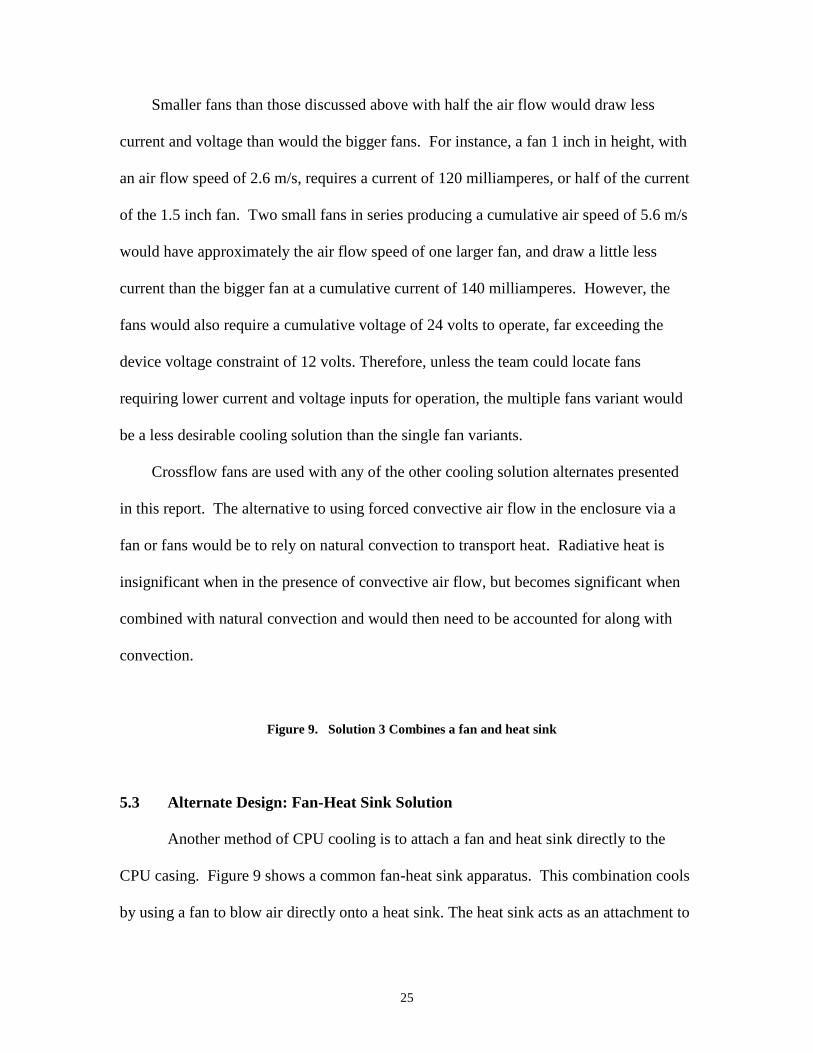
5.3 Alternate Design: Fan-Heat Sink Solution

Another method of CPU cooling is to attach a fan and heat sink directly to the

CPU casing. Figure 9 shows a common fan-heat sink apparatus. This combination cools

by using a fan to blow air directly onto a heat sink. The heat sink acts as an attachment to

Figure 9. Solution 3 Combines a fan and heat sink

26

the CPU case thereby increasing its surface area. This thermal management device has

the ability to move heat, but not re-circulate cool air from outside the motherboard

enclosure. The fan increases the coefficient of heat transfer at the fin surface, allowing

more heat to be dissipated. More convective heat transfer is achieved by constantly

recirculating cool ambient air from outside the enclosure.

The action of blowing air onto a surface at close proximity is called impingement.

This method is more effective than blowing air from a distance at a heat sink. Figure 10

shows that as air hits a surface, flow is decelerated along the z direction and accelerated

along the x direction to conserve momentum. The deceleration continues until the flow

becomes stagnant. At the stagnation point, heat is transferred to the momentarily still air

before it is moved away along the channels of the heat sink.

Figure 9: Impinging fan with heat sink.

27

The action of the fan blowing directly onto the heat sink can be modeled as an array of

slot jets blowing onto an irregular surface. Figure 11 shows an example of a typical slot

jet arrangement. To complete the model, it is important to model the heat sink as an

irregular surface as shown below in figure 12. The larger the surface area the jet

impinges, the greater the convective heat transfer.

Assuming that cooling only occurs in the region directly below the fan, heat is transferred

from the top of the chip to the heat sink by conduction where it is then transferred to the

air blown via forced convection. Convective heat transfer in this case is increased by

having an irregular surface that increases the surface area. The speed and the

Figure 5: Impinging jet model [Incropera, 1996].

28

temperature of the air exiting the fan also increase the coefficient of heat transfer.

Forced convection is governed by the equation

)( ∞−= TTAhQ s

Figure 11: Slot jets cooling a surface [Incropera, 1996].

Figure 12: Important dimensions for modeling the heat sink as an irregular surface.

29

where ≡h average coefficient of heat transfer, A≡ surface area being cooled,

≡sT average surface temperature, and ≡∞T temperature of the air inside the enclosure.

In order to determine the nature of the convective heat transfer, it is important to

determine h . To find h , we must first use an equation that determines the average

Nusselt number of an array of slot jets.

66.0

0,

0,

42.075.00,

Re2Pr66.0

+=

r

r

r

rr

A

A

A

AANu

In this equation, Pr is the Prandtl number (a constant for air at ∞T ),

S

WAr = and

5.02

0, 22

460

−

−+=W

HAr

are area correlation for the slot jet array,

k

DV h∞=Re

is an equation to determine the Reynolds number. In this equation, ∞V is the speed of the

air exiting the fan, k is the thermal conductivity of the air inside the enclosure, and hD is

the hydraulic diameter determined by

WDh 2=

Solving forNu , an average coefficient of heat transfer (h ) can be found using

k

DhNu h=

30

As an example, assume we use a fan-heat sink that is 40 mm square and provides

s

mV 00.2=∞ . Using the equations above, if the chip dissipates 7=Q watts, we can lower

its surface temperature to sT =130°C. A spreadsheet model for this solution is presented

in appendix D to accommodate different CPU sizes. The model can either determine an

approximate temperature that the CPU case could be cooled to based on a known heat

dissipation for the chip, or it can estimate the heat dissipated by inputting the desired

temperature to which we would like to cool the chip.

It is important with this setup to mount the heat sink onto the CPU correctly to

achieve a tight fit between the bottom of the heat sink and the top of the CPU case (see

figure 13). An interfacial material is usually inserted between the boundaries to improve

Figure 13. The interfacial material greatly decreases the thermal resistance between the CPU and the heat sink created by the air gap porosity.

31

the thermal conductivity by removing the air gap created by the adjoining surface

finishes. The interfacial compound is usually an adhesive, but could also be a grease, or a

metal foil. Each of these has varying thermal resistance and each one has benefits over

another. Insuring a tight fit decreases the thermal resistance between the top of the CPU

case and the bottom of the heat sink, thus allowing heat to readily dissipate across the

boundary.


Good features of this solution are that it meets all of the functional requirements

for a cooling method described in appendix A. Listed below are some of the other good

features of this solution:

• low cost if purchased in bulk

• can be purchased with the interfacial material already applied to the heat sink

• no initial tooling cost

• draws less than 200 mA of current

• operate with little noise

• has excellent material integrity (usually made of plastic and aluminum)

• only three assembly steps required

• cools the surrounding circuitry

• is available in different sizes to meet geometry constraints

The three steps required for installation are the heat sink clip attachment, the tightening

of the heat sink to ensure proper contact pressure, and the wiring of the fan to the power

source (assuming power is routed for a fan).

32

Bad features of this solution are:

• limited life expectancy

• contains moving parts

• requires power to operate

• requires a minimum head space of 0.4 inches (to allow proper ventilation)

The typical life expectancy of a fan that would suite our needs is 5 years. But

replacement would be relatively easy but would require opening of the enclosure. Since

the fan contains moving parts, anything that broke off inside the enclosure could get

caught in the fan rendering it useless. Unfortunately, it may be difficult to sense that the

fan is broken before the CPU is damaged.

5.4 Alternate Design: Heat Pipes

One of the viable cooling methods that the team has researched is cooling through

the use of heat pipes. Heat pipes offer the energy transfer method of evaporation and

condensation without needing to submerge circuitry in liquid. A typical heat pipe can

have an effective thermal conductivity 100 times greater than that of a pure metal pipe

the same size. Currently, heat pipes are well known for their use in the cooling of laptop

computers. The main reason for the use of heat pipes in laptops is their size constraint.

Since most laptops are only about an inch in height (the part of the laptop where the CPU

is located), it is not possible to use the fans and large heat sinks found in normal CPUs.

Heat pipes, being small and bendable offer an excellent solution to this problem. Due to

the similarities in size constraints between laptops and DAQ’s, cooling via heat pipes

seem to the team to be a very good method to consider [Graebner, 1999].

33

Heat pipes are thin, hollow, vacuum-tight tubes, usually just a few millimeters in

diameter, which contain a small amount of liquid (usually water). The heat pipe is

composed of a highly conductive metal, often copper, which can efficiently conduct heat

to and from the heat pipe enclosure. When the pipe is placed on top of a chip, the heat of

the chip is conducted to the liquid contained in the heat pipe. As the liquid heats up, it

evaporates (see figure 14). Since the heat pipe is airtight, the hot evaporated liquid forms

a pressure gradient. This causes the vapor to move to the cool section of the pipe, which

is often attached to a heat sink. As the vapor moves, it travels through the open central

part of the pipe (see figure 14). When the vapor cools, it condenses back into a liquid

and, in doing so, releases its latent heat of vaporization (figure 14, C). This process

removes considerable amounts of heat. Because of this large amount of heat transfer from

the pipe, a heat sink large enough to accept the heat must be present. After the vapor

condenses back into a liquid, it returns to the hot end of the tube through the heat pipe

“wick” (figure 14,D). The wick is usually located along the inner surfaces of the tube

and is shaped such that it causes the liquid to return via capillary action. Different wick

types include screen wicks, groove wicks, and powder metal wicks. Each wick has its

own good and bad points. For example, powder metal wicks are limited by the pressure

drops in the tube, yet they can easily transport the liquid back against gravity. On the

other

34

hand, grooved wicks can transfer high heat loads, but can’t transfer large loads against

gravity [Garner, 1996 ].

Thermacore, a manufacturer of heat pipes, conducted a study with Intel to test the

effectiveness of using one of their heat pipes in a laptop set-up with the heat pipe routed

to an outside aluminum plate. The method used to cool this was plate was natural

convection in an ambient environment of 38 °C. The study used a laptop with a mock

chip of 6.54 watts with an additional four watts at four other points within the enclosure

surrounding the chip. The heat pipe was able to keep the chip at 90 °C, 10 degrees

below the stipulated value. In addition to this, the heat pipe was able to dissipate up to

Figure 14: Heat Pipe [Garner, 1996].

35

7.83 watts while maintaining the chip at less than 100 °C. Although this is just one

scenario, it gives us an idea of the amenities that come along with using heat pipes

[Toth].


Heat pipes are not only small, with diameters of a few millimeters and lengths

ranging from a few to several centimeters, but they can also be bent and curved to move

around obstructions. This makes them well suited to the environment of the DAQ box.

Heat pipes are passive devices. This means that no power input is required for heat pipes

to operate, and hence, power of the device is conserved. Although, in some cases, fans or

blowers are required to cool the plate or sink attached to the pipe, this is not always the

case. Heat pipes, being self contained devices have an expected life of many more years

than the DAQ itself is required to function. In fact, the only conceivable way of the heat

pipe permanently failing is if it were to be punctured or broken. Because of the fact that

the heat pipe will not be moved or even touched once installed, this seems unlikely to

happen. Finally, heat pipes are able to satisfy a very wide range of temperature

requirements.

Heat pipes are small, but it should be noted that they do not rid the enclosure of

heat, but rather transfer the heat to other locations. For this reason, heat sinks or

spreaders are required for the heat pipe to attach to. Based on the amount of thermal

resistance required of the heat pipe, the size of the heat sink or spreader can be

determined. Often, several parallel fins or plates are attached to the end of the heat pipe

in order to spread the heat out over a large area. Frequently, the natural convection

36

encountered by these plates is enough to keep the enclosure within the required range.

However, depending on the size limitations, fans may be needed. This leads to another

potential difficulty: “Can a fan that fits the size constraints produce the required

velocity?” As it turns out, this is usually not a problem because in most typical scenarios

where fans are needed, the required velocity is rather low (+/- 1 m/s) [Garner, 1996].

Since heat pipes have become so widely used in the laptop industry, their price

range has dropped dramatically, making them much more competitive with other cooling

devices. Purchased in small quantities (100), heat pipes cost $ 20 dollars per pipe. When

bought in bulk (300,000), heat pipes can cost as little as $4 per heat pipe. Special

amenities such as pipe bends will increase the cost but only by fifty cents per bend (on

average). Adding fins, sinks, or mounting plates may also increase the cost of the pipe

[Toth]. The team has estimated, however, that the entire package required for cooling a

DAQPad via heat pipes (i.e. the pipe, the sink/spreader, and the fan) will cost well below

our required cost of fifty dollars [Toth].

Since the heat pipes are purchased self-contained, and may be purchased pre-

assembled when fins, sinks, or mounting plates are used, the expected cost for tooling

should be low if any cost is needed at all. In most cases, the heat pipe, using a mounting

plate, may be snapped directly onto the chip without requiring any other assembly steps

[Toth].

As with sinks and sink/fan combos, the issue of contact resistance also comes into

play. The same type of contact resistance that is an issue with sink-chip interface is also

an issue with the pipe (or mounting plate) – chip interface. The same type of interface

compounds that are used with heat sinks are applicable with heat pipes [Graebner, 1999].

37

Other problems encountered with heat pipes deal more with operating the pipes at

ranges not specified for the specific pipe set-up. In other words, if the pipe being used is

designed for a certain temperature and wattage range, it should be used in that range.

Problems may occur if the pipe is used outside of its range. One example of this is wick

“dryout”. This wick “dryout” occurs when the maximum power throughput of the heat

pipe is exceeded. The maximum power throughput also referred to as the “dryout power”

occurs when the evaporation rate is greater than that of the resupply of the condensed

liquid. When this occurs, the wick dries out and the pipe no longer operates as a two

phase heat transfer device, but rather as a simple metal tube [Toth].

5.4.2 Preliminary Calculations

As with modeling of any of our variants, basic conditions must be considered

before any calculations are done. These conditions include the required junction

temperature, the ambient temperature, the wattage dissipated by the chip, and the various

resistances of the system. One way to figure out what heat pipe conditions are needed (ie:

diameter required, velocity required, fin array required, etc.) is to solve various scenarios

for the resistance required for the specifications to be satisfied. Typical heat pipe set-ups

for laptops which transfer the heat to an aluminum plate “spreader,” and require only

natural convection to operate, have an effective thermal resistance between 4 and 6 °C/W

for the six to eight watt range. Although, if large heat sinks are used, the resistance can

drop to as little as .2 °C/W for the 75 to 100 watt range [Garner, 1996]. With these

values in mind, the required resistance can be calculated and compared to these values. If

the required resistance is around the 4 to 6 °C/W range, this would probably imply that

38

the set-up could be cooled through natural convection using either a spreader or a heat

sink. However, for lower values, larger heat sinks with forced convection can be

assumed as necessary. Appendix C shows the required resistance for a wide range of

scenarios in which wattage, chip size, and ambient temperature values are varied. These

required resistances assume that the desired junction temperature is 110 C. In the case of

the heat pipes, these calculated values are figured for a heat pipe with a clip-on mounting

plate (i.e., contact is made over the entire chip surface). The value being calculated,

entitled “chip-to-sink resistance,” is equivalent to the required resistance of the heat pipe.

Also included in this appendix is a graphical representation of the required resistance

versus power for three different ambient temperatures. The length of the chip represented

in the graph is .95X.95 inches. The range of values represented in this appendix is what

the team has foreseen as possible values for future DAQPads. The reader may note that

the great majority of these scenarios fall within the range applicable to heat pipes. It

should also be noted that the 90 °C value was included for achieving worst-case values.

It is not expected that the enclosure ambient temperature would actually get this hot; but

rather closer to the 70 °C value.

Another method discussed by Garner for determining heat pipe effectiveness is to

calculate the possible ∆T based on the pipe specification, where ∆T represents the

increase in temperature from the cool end of the heat pipe to the hot end. This is done

using the resistances at the evaporator and condenser portions of the pipe as well as the

resistance due to axial vapor flow.

∆T can be calculated as follows:

condcondaxialaxialevapevap RqRqRqT ×+×+×=∆

39

where:

Revap and Rcond are the resistances at the evaporator and condenser and Raxial is the axial

resistance (i.e. the resistance to axial vapor flow). Rough values to use for these

resistances are .2 °C/W/cm2 for the evaporator and condenser and .02 °C/W/cm2 for the

axial resistance. Aevap and Acond are the heat input areas (the surface area) at the

evaporators and condensers. Aaxial is the cross sectional area of the heat pipe vapor space.

Finally, qevap, qcond, and qaxial are the evaporator, condenser, and axial heat fluxes,

respectively. In an example given by Garner, the condenser and evaporator have the

same length and hence, the fluxes are the same for both parts. For our team’s application,

a conservative estimate for the heat being dissipated is 10 watts with a length of 15 cm

and an evaporator and condenser length of 2cm. Calculating for a .4 cm diameter pipe,

with a .3 cm vapor space,

and hence:

condcond

vaporaxial

evapevap

AQq

AQq

AQq

/

/

/

=

=

=

2/6.79 cmWqaxial =

.2.3 CT °=∆

2/98.3 cmWqq condevap ==

40

The temperature of the cool end of the pipe is dependent on what method is used to

dissipate the heat. If an array of fins with forced convection is used, a significant cooling

of the chip can be achieved. This is just one scenario. Other scenarios for different

wattages and heat pipe sizes can be seen in Appendix E. These values assume the vapor

space diameter is .1 cm smaller than the pipe diameter. Accompanying this table is a

graphical representation of the change in temperature versus power for various pipe

diameters [Garner, 1996].

5.5 Alternate Design: Thermal Electric Coolers (TECs)

Thermal Electric Coolers are effective solid state heat pumps that use small

electric currents to motivate the transfer of heat across its plate faces. The device relies

upon the lesser-known physical phenomenon caused by the movement of current through

a semiconductor material, known as the Peltier Effect. A wire connected to one end of a

stack of “n” and “p” type semiconductor material supplies current to a TEC. The

semiconductor material stacks, made of the compound bismuth telluride, are alternately

doped with excess electrons (n-type junction) or a deficiency of electrons (p-type

junction) to facilitate the transfer of electron current to copper plates connecting the two

types of stacks. Current running through the junctions of this kind of device creates a

temperature gradient between its semiconductor junctions. Single TECs can be stacked

one atop another in “stages”, increasing the overall temperature gradient developed

between the outer face plates. The plates develop temperature gradients ranging from 65

oC for single stage TECs to 131 oC for multistage TECs [Melcor Thermal Solutions

catalog, 1999]. The TEC absorbs heat on its cold plate face and rejects transported heat

41

out through its hot plate face. This heat must then be moved by another cooling solution

in conjunction with the TEC.


TECs are advantageous cooling solutions. They produce no noise throughout

their operation, as they have no moving parts. They are of very compact design. A

single stage TEC can have a surface area of one inch squared and a height of an eighth of

an inch, while a multistage TEC can have a surface area of one to two inches squared and

a height of a half of an inch. The space between circuit boards is optimally constrained to

be 0.5 inches, and many of both the single stage and multistage TECs fit within this

height. TECs work in any physical orientation, which is an especially pertinent issue for

the team to consider when a device is air-cooled and an inverted physical orientation

results in a change in the stability of the air density distribution within the device

enclosure (rising hot air blowing up into an inverted circuit board). The TECs avoid this

air density implication because they conduct heat through a solid medium with constant

density rather than convect heat energy through the air, which has a density dependent

upon its temperature. Single stage TECs can pump 2, 20, or 50 watts of heat energy

away from vital circuitry, while multistage TECs usually pump lower wattage, on the

order of 10 or 20 watts of heat energy, in order to produce a greater temperature gradient

across the TEC plate faces. Although most TECs are designed to cool room temperature

components to subzero temperatures, the team found that the Melcor ThermaTEC was

designed to cool components of up to 200 oC, and could cool components down by 70 oC,

without melting. Because the team anticipates that the chip will have a surface

42

temperature of about 150oC, the TECs designed for subzero temperatures have

components with low melting temperatures that would melt while in contact with the

chip, and would therefore not be useful. Single stage TECs can be purchased in bulk

quantities of 100 or more from between $12.60 for the ThermaTECs up to $30.00 dollars

for other models. The multistage TECs in bulk quantities of 25 or more can be purchased

for around $150.00 dollars. Compared to other cooling solutions, this is relatively

expensive, but the ThermaTEC is affordable (less than the team’s $50 dollar cooling

solution upper limit cost constraint). When used in conjunction with one other cooling

solution, the total cooling solution price does not increase significantly, as fans can cost

around $5.00 dollars in bulk quantities, and heat sinks cost around $2.00 dollars in bulk

quantities. Therefore, price, heat rejection properties, geometry, and physical operation

make TECs a smart cooling solution.

Additionally, TECs can develop serious problems for the board circuitry by

condensing the humidity in the air on the TEC’s cold face plate. The resultant condensed

water corrodes metal leads and shorts the circuitry of the board and the TEC electrically

and thermally [Melcor Thermal Solutions catalog, 1999]. In order to prevent this

condensation from occurring, TEC vendors offer epoxies, silicones, and dip epoxides that

coat the TEC and protect it. Because of temperature limitations, the best combination of

sealants are the silicone perimeter sealant with a maximum temperature usage at 204 oC

and the dip epoxide coating sealant with a maximum temperature usage at 150 oC.

Unfortunately, there are also drawbacks to using TECs as cooling solutions. The

TEC is capable of transporting heat energy from a processor chip (much like the heat

pipe cooling solution), but is ultimately incapable of removing heat energy from the

43

enclosure or itself. It is conceivable that the hot face plate of a TEC could be mounted

next to the enclosure wall, thus conducting its rejected heat into the enclosure to be

convected away into the ambient air. However, due to the anticipated stacked setup of

the circuit boards in the enclosure, this possibility seems to the team remote. Therefore,

each TEC would logically be used in conjunction with another cooling solution.

TEC industry literature suggests that the team should mount a heat sink to the hot

face of the TEC and blow cool convective air across the sink [Marlow Design Guide,

1999]. Because each mounted surface on top of a circuit board component supplies an

additional layer of interfacial heat resistance of conduction (micropores on the surface of

materials contain air pockets, which act as a heat insulators), the introduction of the TEC

as an additional conductive heat resistor reduces the effectiveness of this heat pump

device. TECs also draw more current than the DAQPad6070E device can supply. The

DAQPad6070E is constrained to provide up to 200 milliamperes of current to a cooling

solution, while the single stage TECs can require from 1 to 2 amperes of current and the

multistage TECs can require from 1 to 5 amperes of current for their operation.

Additionally, if, as the literature has suggested, a fan is employed to convect heat away

from a mounted sink, then additional current would need to be drawn from the board to

power the fan. Even with natural convection acting as the ultimate heat transporting

mechanism for the DAQPad6070E circuitry, the above TEC current requirement renders

the Thermal Electric Cooler alternate cooling design less advantageous than other

designs.

The need for sealants is another serious drawback to TECs, and although these

polymers can protect the TEC, there is no way to guarantee that airflow through the

44

enclosure will be sufficiently dry such that moisture will not condense onto the processor

or the circuit board because of the presence of a cold plate face. Sealants also supply an

additional layer of interfacial heat resistance of conduction, which reduces the

effectiveness of the TEC even further. Therefore, unless the team takes the sealant

limitation into consideration when using TECs, condensation is an additional drawback

that is not negligible.

TECs can be used in conjunction with any of the other cooling solution alternates

presented herein.

VI. Experimentation

6.1 Justification for Testing

The design team found that their research material and heat transfer models

pertaining to the heat transported from enclosed microprocessors was an insufficient

source for quantitative processor temperature data. The team made assumptions upon

which they based their heat transfer models, which are stated in the text references as

being accurate to at most 20 percent from actual values for the flat plate Reynolds

numbers and Nusselt numbers, and for the circuit board temperatures of the modeled

circuit board [Fundamentals of Heat and Mass Transfer, 1999]. Therefore, in order to

determine proper cooling method variants based upon more accurate data, the team

decided to design and conduct temperature measurement experiments of a simulated

DAQ circuit board, a simulated microprocessor chip, and a simulated enclosure, as

suggested by their sponsor at National Instruments. The team conducted experiments to

45

find trends in the data from these test measurements and to use these trends to recognize

power ranges over which each cooling method would be appropriate.

The team concentrated their analyses on five main cooling components: heat

sinks, heat pipes, spreaders, crossflow fans, and impinging fans. The team often used

spreaders in conjuncture with, or as an alternative to heat pipes. These spreaders also had

a low thermal contact resistance at their junction with the simulated processor chip, as

they typically do with real processor chips. The team could not account for the

problematic cost and power constraints of thermal electric coolers, and thus the team did

not test these devices. The team had previously decided that heat sinks were likely to be

used in the end cooling solution, whether the team would attach them directly to the

processor chip, or they would use them to cool the end of a heat pipe. Heat pipes were

extolled in the team’s research material as extremely effective cooling components, and

are often used in laptop computers designed with many of the constraints for which the

team’s DAQPad was designed. Spreaders were often used in conjuncture with, or as an

alternative to heat pipes, and spreaders also had low surface contact resistance at their

junction with real or simulated processor chips. Crossflow fans were already tested in the

original prototype DAQ6070E “pizza box”. The team wanted to include this original

cooling method in their tests, in order to have a basis for comparison between the original

cooling method and the team’s test results. The team considered impinging fans to be

more effective in cooling the heat pipe component than the crossflow fans, because the

static pressure impinging heat transfer effect at the heat pipe surface is greater than the

heat transfer in simple convective flow. Also, the team realized that forced convective air

flow would be more efficient than natural convective air flow in removing heat from heat

46

sinks, heat pipes, and spreaders, but the team tested both natural and convective flow in

order to insure that the analysis of the cooling methods was complete. Thermal Electric

Coolers were not considered because of the previously discussed cost and power

constraints. For the reasons above and for those reasons mentioned previously in this

report, the design team was justified in performing temperature measurement

experiments of a simulated DAQ enclosure in order to gain a more sound understanding

of the effectiveness of each of the cooling solutions.

6.2 Test Setup 6.2.1 Description of Chip Simulation In general, depending upon the type of microprocessor on a DAQ circuit board,

and depending upon the work load applied to the microprocessor, each DAQ board can

expel anywhere from 5 watts of power for typical DAQs up to 25 watts of power for

DAQs that have more advanced microprocessor chips [Paulina Mosley, National

Instruments]. The team set out to simulate a typical power output within the range above

from a DAQ main processor chip and a DAQ circuit board. Although the team’s design

specifications required that the team consider board power ranges and chip power ranges,

and not specific board power values or specific chip power values, the team decided that

it would simulate a board and chip power output of 16 watts, which was an approximate

mean power output between the 5 to 25 watt range set in the specification sheet.

47

In order to simulate a 16 watt DAQ, the team chose an assortment of resistors to

serve as heat dissipators. The team simulated the main processor on a DAQ circuit board

by mounting a 10 watt resistor on a non-functioning circuit board (see figure 15). The

resistor was ½ of an inch tall, which was about three times the height of a typical

processor. In order to insure that their tests would produce reliable results, the team had

to find a way to lower the resistor height to approximately match the height of a

microprocessor. The team drilled a hole approximately the size of the 10 watt resistor

into the center of a socket 7 chip socket of the non-functioning circuit board, and fit the

resistor into the drilled hole (see figure 16).

Figure 16: Socket-7-socket with drilled hole.

Figure 15: 10 watt resistor used to simulate chip.

48

The team lowered the resistor into the hole, such that the top of the resistor was flush

with the top of the socket 7 chip socket. Both ends of the resistor needed to be covered in

order to simulate the flat surface of a microprocessor, so on the bottom of the resistor the

team mounted a rectangular section of circuit board about the size of the resistor, which

the team cut from another non-functioning DAQ board (see figure 17). The team placed

ordinary duct

tape around the resistor bottom and cut circuit board, to seal the interface from

convective air flow and to secure the two components together. On the top surface of the

10 watt resistor, the team left the resistor uncovered, or the team covered the resistor with

a heat sink or spreader plate, depending on which test the team conducted. The sides of

the socket 7 chip socket served as the simulated microprocessor side surfaces, and the

components covering the resistor served as the simulated microprocessor top interfacial

surface.

Figure 17: Rectangular circuit board section.

49

The team simulated the remaining 6 watts of the simulated 16 watt DAQ by

soldering a parallel network of half-watt resistors in parallel with the 10 watt resistor.

The team laid the circuit board containing the 10 watt resistor with the resistor top facing

upwards. They then attached one half of the 6 watt resistor network on this board with

thermal tape. The remaining half of the resistor network was attached with thermal tape

to the face of a second non-functioning circuit board. The two networks were connected

by two inch-long insulated copper wires. The second circuit board was placed facing

downwards as was shown in the computer drawings that the team's sponsor had

previously supplied the team. The team spaced the boards by duct taping a one-inch long

piece of chalk at each of the four corners of the boards. The chalk insulated the boards

while still allowing the team access to the resistor network and "chip" resistor between

the boards.

Figure 18: Resistor network and 10-watt resistor.

50

The team used two circuit boards for this layout for three reasons. First, the

team’s specifications were that their cooling methods could accommodate between one

and three circuit boards. Second, a few of the cooling method components would not fit

between the circuit boards inside of the team’s simulated 1.7 inch tall enclosure if the

team simulated three circuit boards in their test enclosure. Third, the team wished to

perform their tests on their simulated DAQ under conditions that would match the team’s

specifications as closely as possible. Therefore, the team chose to simulate the cooling of

two circuit boards, and they were then able to fit all of the cooling method components

that they wished to test between the circuit boards. The resistive network that the team

laid across the circuit board faces represented the simulated elements on the board that

dissipated heat. The team felt that this resistive network would realistically effect the

heat dissipation of the simulated microprocessor 10 watt resistor.

6.2.2 Back-Calculations for Estimating Junction Temperature

As mentioned, for our experimentation, the team modeled the main processor chip

using a resistor. In the physical set-up, the resistor acted as the chip case. For our

various tests, the heat sinks, heat pipes, and impingement coolers were mounted directly

onto the resistor just as they would be mounted onto the actual chip case in a real

DAQPad. However, unlike an actual chip case, the resistor itself was generating the heat.

In an actual DAQPad, the junction, located inside of the chip case, would be generating

the heat. Furthermore, this junction temperature is usually what is of interest to chip

manufacturers; and is usually the part of the chip that has operable temperatures specified

for it. Since temperature readings were taken from the mocked chip surface, back-

51

calculations were needed in order to estimate what the hypothetical junction temperature

would be. The specified ambient temperature range for National Instrument's DAQPads

is between 45°C and 55 °C. However, the team performed their experiments in an

ambient temperature of 25 °C. For this reason, additional calculations were needed to

estimate the junction temperature at the ambient temperatures specified for the DAQPads.

The resistance model shown in figure 19 represents the heat transfer flow between

the chip junction and the heat sink/ heat pipe mounting plate. θCS is the resistance

between the chip surface and the heat sink/heat pipe mounting plate. This resistance was

modeled in experimentation as the resistance between the resistor and the heat sink/heat

pipe mounting plate. It is important to note, however, that cross sectional area of the

resistor is only about .125 square inches. This area is much smaller than a typical chip

case contact area which typically ranges between .9 in2 and 4 in2. Because of this fact, it

Figure 19: Resistance diamgram for heat flow between junction and heat sink/heat pipe mounting plate.

THeat Sink/Pipe mounting plate

TJunction

TCase

θJC

θCS

52

.is likely that the actual junction temperature of a chip will be slightly cooler by a few

degrees than that which we have calculated by a few degrees. θJC is the resistance

between the junction and case of the chip. This is the additional resistance that needs to

be considered when back-calculating the junction temperature. To obtain conservative

values, the team decided to use a worst case value of 2C/watt for this resistance. Hence,

for every watt dissipated by the resistor, 2 degrees celcius would need to be added to the

temperature reading of the resistor, taken by the thermocouple in order to obtain the

estimated junction temperature.

Since the ambient temperature and the junction temperature rise in a linear

relation to each other, the difference between experimental ambient temperature (+/- 25

°C) and the specified ambient temperature (45° – 55°) would also be the difference

between the junction temperatures in each of these ambient conditions. Since the

experiments were run at an ambient temperature of approximately 25 °C, 20 – 30 degrees

below the specified range, 20 or 30 degrees should be added to the junction temperature

to obtain the estimated temperature of the junction in that ambient environment.

Based on these two aspects that are required to calculate the hypothetical junction

temperature, the following equation was derived by the team:

Ambientjcresistorjunction TQTT ∆+×+= θ

Where:

Tjunction = the temperature of the hypothetical chip junction

Tresistor = the temperature of the resistor (mock chip)

Q = the heat dissipated by the resistor (mock chip)

53

θjc= the thermal resistance between the junction and chip case

∆Tambient = The difference between the ambient temperature specified for the

DAQPad by National Instruments (45 – 55) and the ambient temperature that the

experiments were conducted in.

An example incorporating this equation and using the “worst-case” value for θjc

is shown below for one of the heat pipe tests that the team performed. In this test, the

resistor temperature was brought down to 54 °C while dissipating 10 watts. To calculate

the hypothetical junction temperature, the following calculation could be performed:

These calculations would reveal that the hypothetical junction temperature (for this

example) in an ambient temperature range of 45°C to 55 °C would range from 94 °C to

104 °C.

.30)/2(10

,

20)/2(10

CWCWTT

And

CWCWTT

resistor

resistor

°+°×+=

°+°×+=

54

6.2.2 Box Design for Experimentation

6.2.3.1 Box Composition

The design team investigated several options for composition of the simulated

DAQ enclosure box. The design team wanted to construct an enclosure that was as

similar to a final DAQPad product as possible, to insure that their tests would produce

reliable results. The team also wanted to choose the enclosure material such that the box

would have favorable thermal and structural properties for during both the construction

and testing phases of the team's experimentation. After speaking with Professor Don

Artiefschoufsky, the Head of the Department of Mechanical Engineering Machine Shop,

the design team decided that their test enclosure would be constructed of nominally 1/16th

inch thick 6061-T2 sheet aluminum.

DAQPad-6020E, a currently manufactured National Instruments DAQ model is

made of a 1/16th inch thick aluminum frame with a 1/16th inch thick paint coating. 6061-

T2 aluminum is commonly used in metal frames like the DAQPad-6020E and is

moderately formable. It has a tensile strength three times less than stainless steel or

beryllium copper, and two times less than plain carbon steel, but the team expected that

neither the test box nor the enclosure would be loaded to a stress anywhere approaching

aluminum's yield strength of 310 MPa. Therefore, the team concluded that aluminum’s

lower strength and elasticity as compared to other materials would be relatively

unimportant in their design of the DAQ test box or the final DAQ enclosure prototype.

Aluminum is also about three times less dense than both copper or steel, and would

55

therefore meet the team's constraint that the enclosure, and by extension the test box, be

lightweight. 6061-T2 aluminum has a thermal conductivity of 180 W/m*K, very close to

2024-T2's thermal conductivity of 195 W/m*K, an aluminum alloy notable for its higher

concentration of copper. Thus 2024-T2 aluminum is favorable for use in heat conducting

machine components [Engineering Materials-properties and selection, 1999], and by

analogy 6061-T2 would be favorable for use in a heat conducting enclosure. Aluminum's

thermal conductivity is about twice that of plain carbon steels, ten times that of stainless

steels, and about one thousand times that of a typical commodity plastic like polystyrene

[Fundamentals of Heat and Mass Transfer, 1996]. Therefore, 6061-T2 aluminum was

thermally superior to all other materials that the team examined. The team also wished to

maximize the time needed to manufacture their test box, and 6061-T2 aluminum was

readily available in Professor Artiefschoufsky's machine shop.

6.2.3.2.1 Dimensions

The dimensions used to build our test enclosure were determined from National

Instrument’s conceptual drawings of their upcoming DAQ model. We chose to make our

test enclosure 5 inches wide to allow enough room for the widest circuit board given to us

by NI. The test enclosure length was set at 10 inches to allow space for the longest board

plus some extra room for the heatpipe testing. A height of 1.7 inches was used to comply

with the industry standard for rack mountable equipment. When deciding on what

dimensions to make our enclosure, we purposely tried to limit our available free space. If

our cooling solution were to take up extra room inside the enclosure, we could extend the

56

length; but we would like to limit our free space to make the packaging more efficient.

Figure 20 below shows a conceptual enclosure design and the corresponding dimensions.

Figure 20: Conceptualized dimensions for the DAQ enclosure.

6.2.3.2 Ventilation

When constructing our test enclosure, we considered the need to properly

ventilate the hot components inside. Venting the enclosure with cool ambient air

improves the performance and can prevent damage due to overheating. NI specifically

asked that we not place ventilation holes on the top, bottom, or sides of the enclosure;

because of the possibility of placing DAQs side-by-side or stacking them on top of other

equipment. Figure 21 below shows three DAQs in a typical testing orientation.

57

Figure 21: DAQs (top row) placed side-by-side.

After researching enclosure designs for electronic components, the team concluded it was

best to use an enclosure with vents to create a circulation of cool ambient air into the

enclosure. If the components inside require more than natural convection, a fan can be

installed at one of the vents to increase the airflow through the enclosure. A fan should

be oriented such that it pulls air from outside the box and blows it into the enclosure. The

most temperature sensitive chip should be placed in front of the fan to ensure direct

cooling by convective heat transfer. Spot cooling of hot components can be achieved by

using a small fan that is triggered when the CPU reaches a certain temperature.

Components with high heat dissipation should be located near the exit vents to reduce the

heating of the air in the enclosure. The exit vent should have the same area as the inlet

vent to avoid pressurizing the enclosure that would reduce the efficiency of the fan and

58

create a recirculation of warm air. Figure 22 below summarizes a suggested ventilation

scheme.

Venting can be accomplished by allowing enough room for vents at the front and back

panels, and covering them with either a mesh or screen to reduce dust and the possibility

of obstructing the fan. Figure 23 below shows an area labeled “A” that could be used to

install a front vent.

Figure 22: A suggested layout to improve box ventilation.

59

Figure 23: The RF connections typically on the DAQ.

6.2.3.2 Board Arrangement

The team chose to arrange the boards inside the enclosure based again on the conceptual

drawings furnished by NI. From the drawings, it appears that two boards needed to be

enclosed.

Figure 24 : The boards inside the DAQ.

Stacking the boards and connecting them with a “bus” allows efficient use of space. One

board arrangement would be to push them closer to the fan or the vent, depending on

what type of components are mounted on the board or the need for extra space

60

6.2.3.3 CPU and Circuit Board Heating

In the previous section on ventilation we discussed the advantage of placing the most

temperature sensitive chip, usually the hottest CPU, closest to the inlet fan. This provides

it with the most convective heat transfer possible by placing the chip in crossflow. To

simulate the heating of a CPU, the team used a resistor to generate the heat. It was placed

in a vacancy created on the board by removing one of the original CPUs. Then we placed

a resistor capable of dissipating 10 watts of heat on the board, to simulate the heating of

an actual CPU chip.

6.2.3.4 Additional Heat Sources

The heat generated during use not only comes from the CPU, but also the other board

components and their circuitry, accounting for as much as 40% of the total heat

generated. To simulate this heat, seventeen 2.2kΩ resistors were connected in parallel

and taped to the faces of the boards. The number of resistors and their corresponding

resistances were determined to output 6 watts. Figure 25 shows the resistor used to

simulate the heat dissipation of the circuit board components and the CPU.

61

Figure 25: The resistors used during testing.

6.2.4 Testing Equipment

After the prototype test enclosure was constructed, the equipment needed to run tests of

heat dissipation were connected. Our sponsor lent us “NI-DEC” which is a virtual testing

bench for taking temperature readings versus time. Along with the software, NI also

gave us a converter box to translate the data sent to the computer by the thermocouples.

Power sources were used to heat the resistors and to power a fan if crossflow or

impingement cooling was tested. A multimeter was used to monitor the voltage to the

resistors to ensure proper heat dissipation. Figure 26 below shows the equipment used

during testing.

62

Figure 26: Displaying the equipment used during the testing phase.

6.2.5 Test Methods

6.2.5.1 Thermocouple Attachment

The team recorded two separate temperature readings for all of the experiments

they performed: the temperature of the main resistor or mock chip case and the “in-box-

ambient,” or the ambient temperature in the enclosure. The more important of these two

readings was the mock chip temperature. This was important because a large percentage

of the heat from a real circuit board comes from the main processing chip whereas the

rest of the total heat dissipated by the system is dispersed out among all the other

components. In order to get accurate temperature readings a small hole was drilled into

the casing of the resistor just large enough to fit the thermocouple wire inside and

63

approximately .25 inches deep (see figure 27). Once the thermocouple was inserted into

the hole, the opening was covered with thermal tape.

The second thermocouple was placed close to the front of the enclosure equidistant from

each of the two boards in the box. Although the thermocouple was not touching the

“other heat sources” (resistors), it gave the team an understanding of the over-all heat of

the enclosure due to the total heat dissipated (see figure 28).

Figure 27: Insertion of thermocouple into resistor.

Figure 28: Placement of thermocouples within test enclosure.

64

6.2.5.2 Wattages Tested

As discussed earlier in this report, the team decided to test a simulated DAQPad

having a total wattage dissipation of 16 watts, with 10 watts dissipated by the main chip.

This was power dissipation was the one which the team used for all of the initial testing.

Later tests focussing on a selected cooling method observed variations in wattage. In

order to determine the voltage required to produce a desired wattage output, the following

relation was used:

Using the desired output power of the chip and the given resistance of the resistor, the

required voltage was determined. This voltage was preset on the voltmeter prior to each

test.

6.2.5.4 Procedure

With the power source preset to the desired voltage, and the thermocouples

situated in their proper locations, the actual test was set to begin. The variant being tested

was placed inside the enclosure. For the heat sink and heat pipe tests, thermal grease was

applied to the face of the resistor which was then attached to the heat sink or heat pipe

mounting plate via screws. In the case of the heat pipe test, the finned, condenser end of

the pipe was directed to the back of the enclosure near the vents. For all experiments run,

R

VP

2

=

65

the resistor was then inserted into the burrow designed in the board in order to minimize

the heat dissipated from surfaces other than the top surface. With the variant in place, the

upper board was then placed over the main board separated by half-inch risers (see figure

29). The back and top panels of the enclosure were then placed onto the enclosure sides

and attached with tape, making sure to leave no air gaps between enclosure faces. With

the leads from the resistors and fans (if applicable) attached, the power source hooked to

the resistors was then turned on and the temperature readings were recorded using

National Instrument's “Virtual Bench” software package, provided by the team’s sponsor.

Figure 8: Test set-up with top board placed over main board.

Figure 29: Enclosure with upper circuit board placed over main board.

66

6.2.5.4 Duration of Tests

Each test was allowed to run until temperature readings leveled off

asymptotically. At this point, if the variant involved forced convection via a fan, the fan

was then activated. Again, the test was allowed to run until the readings leveled off

asymptotically. This method allowed the team to view how effective each cooling

method was utilizing natural as well as forced convection.

6.2.6 Description and Analysis of Variants Tested

6.2.6.1 Natural Convection Cooling of the 10 Watt Resistor

The team began testing their simulated DAQ enclosure by powering the 10 watt

resistor and the 6 watt resistor network inside of the DAQ device to their listed maximum

power ratings. They connected the resistors to a power supply set to provide 28.9 volts

across the parallel circuit. This voltage corresponded to a cumulative power flow through

the resistors of 16 watts. These values were based upon the team’s electrical power

calculations for the simulated chip resistor and the resistor network. Immediately upon

powering the resistors, and after setting up each test, the team adjusted the National

Instruments "Virtual Bench" software to begin recording or "logging" their desired

temperature data readings of the simulated DAQ test box.

The team allowed the resistors in the test box to accumulate heat. They placed the

thermocouple that measured the ambient temperature in the test box toward the front as

discussed previously. They fastened the thermocouple that measured the 10 watt resistor

directly to its top surface using a small strip of thermal tape. The design team did not use

67

a cooling method for the natural convection tests. The circuit boards and the test box

conducted heat away from the resistors, and the air inside of the test box whisked away

heat by natural convection through vents in both the front and back face plates of the box.

Conduction through the circuit boards was present throughout each of the team’s cooling

method tests, but natural convection had a negligible affect upon the resistive elements

within the test box when forced convection was present.

Natural convective and conductive heat transport through the circuit boards in the

test box, in addition to the team’s constraints in the specification sheet, was the basis

upon which the team judged the results of their cooling method tests. In all of the tests

that the team conducted, including the natural convection base case, the team allowed the

resistors in the test box to accumulate heat, such that the “Virtual Bench” software

temperature plot of the powering up 10 watt resistor increased in a positive exponential

manner. This exponential behavior of the temperature of the resistor did not surprise the

team, as several examples of exponential models of temperature distribution and heat

transport are developed for both transient conduction and internal fluid flow in the

reference texts [Fundamentals of Heat and Mass Transfer, 1996]. In fact, the team

assumed that the transient behavior of the resistor during its heating period would closely

simulate the transient behavior of a microprocessor initially powering up.

The team ran their base case natural convection test. After the team powered up

the resistors, the internal ambient air in the test box reached 45 oC. The 10 watt resistor

reached a steady state asymptotic temperature of approximately 304 oC. According to the

team’s design constraints, the temperature of the 10 watt resistor, 304 oC, was

unacceptable. Graphical results can be seen in Appendix G-1.

68

After conducting a base case natural convection test, the design team considered

natural convection from a heat sink that they attached to the 10 watt resistor. The team

drilled two holes into the bottom of an aluminum heat sink that they had obtained through

Thermalloy Incorporated, a prominent heat sink vendor (see figure 30). The team next

removed the 10

watt resistor from the circuit board and inserted threaded fasteners through the two eye

holes in its aluminum casing. The team tightened the threaded fasteners and connected

the 10 watt resistor to the aluminum heat sink, making sure to apply a dab of thermal

grease into the interfacial space between the resistor and the heat sink (see figure 31).

They reinserted the resistor into the circuit board and connected the resistors as before.

Figure 30: Heat sink with holes drilled.

Figure 31: Heat sink connected to heat sink.

69

The team ran two tests to measure the steady state asymptotic temperature of the

resistor with an attached aluminum heat sink. For the first test, the team attached a

thermocouple to the long side of the 10 watt resistor with a small strip of thermal tape.

Because this connection was not located at the interface of the heat sink and the resistor,

the team expected to obtain temperature readings that would inaccurately portray the

microprocessor junction temperature. One method to overcome this obstacle, as

described to the team by their sponsor, is to drill a hole into the heat sink and to set a

thermocouple lead into the hole, just above or just touching the chip or resistor case. In

order to stabilize the position of the thermocouple lead, the thermocouple is then fastened

into place using an epoxy. The sponsor emphasized to the team that the setup time for

running this test would be excessive. The team assumed that this suggested temperature

measurement method was effective for use in testing the performance of a functioning

DAQ circuit board. However, because the team was testing a simulated DAQ circuit

board, because the team wished to minimize their heat sink test setup time, and because

the team would be unable to reuse an epoxied thermocouple (of which they had a limited

supply) for other cooling method tests not involving the heat sink, they chose to measure

the resistor case temperature at separate locations in two separate tests: they measured the

temperature at the long side of the resistor in their first test, and they measured the

temperature at the base surface of the heat sink in their second test. However, the team

only used the data from the second test, as that test resulted in more conservative values,

and the team felt that measuring the temperature of the heat sink was more accurate.

At the beginning of their test, the ambient temperature inside of the box, the

temperature of the resistor, and the temperature of the heat sink were about 28 oC. The

70

team attached the thermocouple lead to the base surface of the heat sink with thermal tape

in the second test, and found that the heat sink reached a steady state asymptotic

temperature of about 130 oC after running the test for 28 minutes. The ambient

temperature inside of the test box for this test climbed in a slow, linear fashion, reaching

a temperature of about 42 oC at the 28 minute-mark. Further results can be seen in the

appendix G-3.

In the test of the 10 watt resistor with an attached aluminum heat sink, the resistor

reached a steady state asymptotic temperature of 130 oC. According to the team’s design

constraints, this temperature was unacceptable. Therefore, the team concluded that

natural convection cooling of the DAQ circuit boards with a microprocessor heat output

of 10 watts, for either their base case, or with just a passive cooling element like a heat

sink, would be unacceptable in the DAQ enclosure prototype. The team concluded that

they would need to include a more active cooling method in their final prototype design

to keep the 10 watt resistor within an acceptable temperature range.

6.2.6.2 Forced Convection Cooling of the 10 Watt Resistor

The team conducted four tests with crossflow convective cooling of the 10 watt

resistor in order to form a base case for convective cooling without a heat sink, to form a

more advanced case of convective cooling with a heat sink, and to check the reliability of

each of these tests. The team powered the resistors, attached the thermocouples, and ran

71

the National Instruments “Virtual Bench” software exactly as they did for the natural

convection tests, except now they also connected a small 1.5” x 1.5” x 0.5” crossflow fan

to a power source set to provide 12 volts independently of the power source connected to

the resistors (see figure 32). The team set the fan in the back of the enclosure, directing

the fan to blow air across the enclosure circuit boards and out the front face plate vent.

The air from the

fan provided a means for convective heat transport from the resistors, from the circuit

boards, and from the enclosure. The team assumed that the fan was relatively efficient

and that its low power usage, about 1.2 watts, was small enough to conclude that waste

heat entering the blown air from the fan was negligible.

The team conducted a forced convective airflow test without a heat sink. For this

test, the team switched on the fan at the beginning, allowing the 10 watt resistor to reach

an asymptotic steady state cooled temperature of approximately 228 oC. The ambient

temperature of the air in the box reached 35 oC. The team noticed that the slight increase

Figure 32: Resistor cooled by crossflow experimental setup.

72

in slope of the plot of this temperature distribution was due to the team turning off the fan

momentarily. Further results can be seen in the appendix G-2.

6.2.6.3 Forced Convection Cooling of the 10 Watt Resistor with a Heat Sink

The team began their more advanced test case of the 10 watt resistor with a heat

sink in forced convective airflow by attaching an aluminum heat sink to the 10 watt

resistor, by attaching the thermocouple leads, and by running their test exactly as they

had done with the natural convection heat sink tests. The ambient temperature of the air

in the test box steadily decreased to a temperature of 33 oC as the fan cooled the 10 watt

resistor. The temperature of the 10 watt resistor decreased from 130 oC to 82 oC. Further

results can be seen in the appendix G-3.

6.2.6.5 Heat Sink With Impinging Fan

One of the variants tested was the use of a fan-heatsink. The heatsink is attached

to the CPU and a fan is placed on top of the heatsink. Instead of providing a crossflow,

the fan blows directly on top of the heatsink creating an impinging effect describe in

section 5.3. Attachment of the resistor to the heatsink was accomplished by drilling and

tapping two screw holes in the bottom of the resistor. After coating the top of the resistor

with thermal grease, it was bolted down to achieve good contact pressure. Figure 33

below shows the attachment of the resistor to the bottom of the heat sink.

73

Figure 33: Displays the fan-heat sink tested.

The thermocouple was then placed into a small hole drilled into the resistor to ensure

proper temperature readings. After placing the impinging fan and resistor into the test

position, electrical tape was then used to cover the gap left between the bottom of the

heatsink and the top of the circuit board. This was done to prevent cooling of the

heatsink from underneath. Testing was done by inputting voltage from the power source

to the resistors. After heating the resistors and allowing them to reach a thermal

equilibrium, the impinging fan was turned on to cool the heatsink until it reached another

thermal equilibrium. It is important to mention that the thermocouple was attached to the

casing of the resistor closest to the contact area of the heat sink and resistor bottom. This

was done to accurately measure the temperature of the resistor. Results can be seen in

appendix G-4.

74

6.2.6.6 Heat Pipe with Aluminum Mounting Plate and Pinned Heat Sink with Fan

6.2.6.6.1 Constricted Ventilation

The last variant tested by the team was that of a heat pipe. Since it was

understood that the heat pipe would be the most effective dissipation, the team decided to

create a worst case scenario for air flow. To do this, the wattage was kept the same, but

the ventilation was altered. The front plate was completely covered, such that no air

could escape or enter from this area. Although more ventilation means a cooler box, the

team recognized that one of National Instrument’s conceptual schematics of the DAQPad

would not allow any room for venting in front of the enclosure. Also, instead of using

screens in the back of the enclosure, a second back-face-plate was used. This plate

consisted of 1/8 “ thick aluminum with several 1/8 “ diameter holes punched out of it. In

addition to this, an aluminum plate was placed between the section of the box where the

circuit boards were located, and the back of the box where the impingement fan was

located (see figure 34).

75

Figure 34: Heat pipe experiment setup.

The heat pipe used for experimentation was sampled to us by Thermacore. It was

a typical electronics cooling copper heat pipe 6 inches long and 6 mm in diameter that

contained water as the working fluid. In order to ensure proper thermal flow from the

mock chip to the heat pipe, a mounting plate was machined in the ETC machine shop.

This plate, designed by the team, was made of aluminum and measured 1.75 inches by

1.75 inches by .25 inches. A hole was drilled into the side of the plated just wide enough

to allow the evaporator end of the heat pipe to be inserted in ¾ of an inch. Two screw

holes were tapped onto the face of the plate that allowed for the mock chip to be screwed

on (see figure35). For the condenser end (the cool end) of the pipe, a pin heat sink 1 “ in

height was selected. This sink also had a hole drilled into its base just large enough for

the condenser end of the heat pipe to fit all the way through. An impingement fan

40mmX40mmX10mm sourcing 12 volts and .06 amps was placed directly over the sink.

This fan was rated at 9.7 CFM (see figure 35).

76

Figure 35: Heat pipe connected to mounting plate and

heat sink with fan.

Upon testing, all interfaces were coated with thermal silicone compound. These

interfaces included the chip-to-mounting plate interface, the mounting plate-to-heat pipe

interface, and the heat pipe-to-heat sink interface. The mock chip was then placed placed

in its proper position with the heat pipe extending to the back section of the enclosure

near the ventilation. In order to fit nicely in the enclosure, the heat pipe was bent to an

angle of approximately 120 degrees. As discussed earlier, an aluminum divider was then

placed between the circuitry and the heat sink/fan at the back of the enclosure to simulate

components that might be blocking air flow in an actual DAQPad. This setup can be seen

in figure 34. At this point, the power supply was attached to the mock power leads and to

the impingement fan, and the voltage was set. The top board was then placed

approximately ½ inch above the main board and the top was sealed onto the box. The

test was then initiated.

As with the other tests, this test was allowed to run without the fan until the

temperature readings leveled off. This occurred at 1 and ½ hours after the test was

started with a maximum temperature reading of 112 C for the mock chip and 50 C for the

77

in-box-ambient temperature. The impingement fan was then turned on and readings were

collected, again, until the temperature leveled off. This occurred approximately 2 hours

after the onset of the test with a mock chip temperature of 66 C. The in-box-ambient was

reduced to 48 C. A graphical representation of this test can be seen in appendix G-5.

6.2.6.6.2 Screened Ventilation

In order to compare the heat pipe method with the other methods, a second test

with the aluminum mounting plate was performed. This test had a ventilation method

identical to the preceding methods. This included the small section in front and the entire

back of the enclosure covered with the screen mesh. This test was run as the others were

with a maximum resistor temperature of 107.5 °C and an in-box-ambient temperature of

40.7 °C without the impingement fan on. After the fan was activated, and the

temperature readings allowed to level off, the resistor temperature was reduced to 55.0 °C

with an in-box-ambient temperature of 33.2 °C (G-6).

6.2.6.6 Heat Pipe with Copper Mounting Plate and Pinned Heat Sink with Fan

A second heat pipe test identical to the initial test with the exception of the

material used for the mounting plate was run. This plate had the same dimensions but

was composed of copper. Since copper has a much higher conductivity than aluminum,

the team decided experimenting with a copper plate might create a lower mock chip

temperature. However, this was not the case. The maximum temperature reached by this

test was slightly higher than the preceding test with a maximum temperature of 118

degrees. The final temperature reached by the setup with the aid of the fan was identical

78

to that reached by the preceding test (166 °C). The results of this test can be seen in

appendix G-7.

6.3 Follow Up Testing at Various Wattages

By noting the cooling capabilities of the various scenarios, the team became

aware that some of the cooling methods would be applicable at different wattages. For

the lower wattages, a spreader or heat sink could be used if necessary. For the middle

wattage values, a heat pipe utilizing only natural convection could be utilized. Finally,

for the upper values including the 16 watt dissipation used in the initial testing

(corresponding to 10 watts from the main mock chip) a heat pipe with impingement flow

could effectively cool the chip. To obtain more data that could better describe the

temperatures reached with a cooling method at varying wattages, the team decided to

perform two follow up tests. Each of theses two tests included the same array of resistors

to simulate the main chip and the “other” power sources (such as power modules and

circuitry). Since the same resistor array of resistors was used , the proportion of power

emitted from the main chip to the total power remained a constant 62.5 % for each

wattage tested. Also, each test included a front enclosure face plate that was completely

sealed (no vents) and the aluminum back-face-plate with holes drilled out of it.

79

6.3.1 Heat pipe with Natural Convection at Various Wattages

The fist of the follow up tests was aimed at observing the cooling capabilities of

the heat pipe utilizing only natural convection at various middle wattage values (8-10

watts for the entire system). Since the initial testing found that the mock chip with the

copper mounting plate reduced the mock chip by essentially the same amount, the team

decided that either mounting plate would be adequate. The same pined heat sink was

used for this test, with the exception that the impingement fan was removed from the sink

to allow no interference of the natural convection of heat away from the heat sink. The

initial power through the main chip was set to five watts (a total wattage of eight watts

for the whole enclosure). The test was allowed to run at this wattage until the

temperature readings leveled off. At this point, the voltage was increased such that the

main chip was emitting 6 watts (total power emitted was equal to 9.6 watts). This

procedure continued also for 7 and 8 watts of power emitted by the main chip. The

results can be seen in appendix H-1.

6.3.2 Heat pipe with Forced Convection

The second follow up test was geared to determine the cooling capability of the

heat pipe with impingement for the maximum suggested wattage of 25 watts. This

required a wattage of 15.6 watts to be emitted from the main mock chip. The testing was

run with the fan activated from the onset of testing, and testing continued until the

temperature readings leveled off. At this maximum wattage suggested by National

Instruments, this method cooled the mock chip to 82.6 °C with an in-box-ambient

temperature of 59.6. The results of this test can be seen in appendix H-2.

80

6.3 Comparison of Test Results

6.3.1 Representation of Recorded Temperature Readings

For comparison purposes, the team compiled a table of temperature values taken

during experimentation for each cooling variant (See tables 3 and 4). These tables list the

steady state temperature readings reached for each experiment with and without the aid of

the fan. The tables show the values actually recorded by Virtual Bench, not those

calculated as the hypothetical junction temperature. For visual comparison, this data was

also put into a bar graph (see figure 36).

Table 9: Recorded in-box-ambient temperatures for variants.

Table 3 : Recorded resistor temperatures for variants.

81

6.3.2 Representation of Calculated Junction Temperature

As discussed earlier, it was desired by the team to back-calculate the hypothetical

junction temperature attainable with each test method. The methods discussed earlier in

this paper were used to arrive at this value. Tables 5 and 6 outline these junction

temperatures as well as the altered in-box-ambient temperatures which were obtained by

adding the difference in test ambient temperature and the ambient temperature specified

by National Instruments to the internal box temperature recorded. A bar graph is also

provided for this calculated junction temperature (see figure 37).

Figure 36 : Bar graph of attainable tempearatures as a function of the variant.

0

50

100

150

200

250

300

350

Chip Alone Heat sink Impingement with sink Heat pipe with nofront/drilled back

Heat pipe with screenvents

Maximum Temperature vs. Variant

Without fan With fan

128.9

82.3

54.066.0

106.6110.5

86.8

132.6

229.3

303.7

82

Table 6 : Calculated junciton temperatures for variants.

Table 5: Table of calculated in-box-ambient temperatures for variants.

Figure 37: Bar graph of maximum junction temperature as a function of the variant.

0

50

100

150

200

250

300

350

400

Tem

per

atu

re (

C)

Chip Alone Heat sink Impingement with sink Heat pipe with nofront/drilled back

Heat pipe with screenvents

Maximum Temperature vs. Variant

Without fan With Fan

353.7

104.0

156.6

178.9

116.0132.3 136.8

160.5

182.6

279.3

83

6.3.3 Representation of heat pipe with natural convection at varying wattages:

actual readings

The results of the follow-up heat pipe with natural convection experiment were

also compiled into a tabular format presented in figure 7. In addition to this, a chart

graphing the wattage emitted by the mock chip as a function of chip temperature was also

plotted (see figure 38).

Figure 38: Graph of Temperature vs. Wattage for passive heat pipe experiment.

Temperature Attained vs. Power Emitted

0

20

40

60

80

100

120

4 5 6 7 8 9 10 11

Power (watts)

Tem

per

atu

re (

C)

Resistor In-box-ambient

Table 7:Recorded resistor temperature and in-box-ambient for various wattages.

84

6.3.4 Representation of heat pipe with natural convection at varying wattages:

Calculated junction temperature

For this follow-up test, the junction temperatures were also compiled into a tabular as

well as a graphical format. These representations can be seen in table 8 and figure 39

respectively.

Table 8: Calculated junction temperature and in-box-ambient for various wattages.

Figure 39: Graph of The calculated Junction Temperature vs. Wattage for passive heat pipe experiment.

Calculated Junction Temperature Attained vs. Power Emitted

0

20

40

60

80

100

120

140

160

180

4 5 6 7 8 9 10 11

Power (watts)

Tem

per

atu

re (

C)

Resistor In-box-ambient

85

6.3.5 Possible Errors Incurred During Experimentation

Although the team attempted to simulate a real DAQPad with their experimental

setup, the team has identified possible areas prone to error. Most of these errors were a

result of the arrangement and dimensions of the mock chip. Ideally, the sides and bottom

of the mock chip needed to be completely insulated to allow for heat transfer solely

through the top of the resistor. This insulated scheme would more accurately model an

actual chip. The resistor arrangement used in experimentation was insulated to a degree

by its placement within the circuit board. However, gaps in this placement of the resistor

allowed some heat transfer to occur at the sides and bottom of the resistor, which would

normally not occur with a real chip. A second cause for error with the team’s

experimental setup was due to the size of the resistor. Since the contact area of this

resistor was only 0.125 in2, which is much smaller than that of a typical chip, a smaller

heat flux would be generated for the resistor.

VII. Results and Conclusions

8.1 Data Trends

The team analyzed the results of their testing and arrived at several conclusions

from which future design of the DAQPad-6070E and other DAQPads might be made.

From examining the temperature versus time plots found in the appendix, the team

concluded that during the initial powering up period of the DAQ microprocessor, the

86

temperature of the DAQ chip and the DAQ circuit board would increase exponentially

with respect to time. This temperature would continue to increase until the main chip

reached a constant temperature. This steady state value would stay constant throughout

the use of the device, so long as the cooling methods employed in the device had been

operating since its initial powering up. If, for instance, the cooling methods employed

were to be turned on after the DAQ device had reached a steady state temperature, then

the device temperature would drop to a new steady state value, which would remain

constant so long as the cooling method employed remained operating. The team

conducted experiments that accounted for this activity, as seen in appendix $$$. Also,

for instance, if a designer chose to employ an automatic mechanism for regulating how

the DAQ device’s cooling methods operated with respect to temperature, turning off

when the DAQ device had cooled down and turning on when the DAQ device had heated

up, then the peak DAQ device temperature value would oscillate instead of remaining

constant. The team did not conduct experiments accounting for this activity, but instead

explained this activity in the recommendations section of this report.

The ambient temperatures in these plots tended to also rise exponentially as the

microprocessor heated to its steady state value, where the ambient temperature reached

its own steady state value. However, whenever the team turned on their tested cooling

method late in the test, after the mocked chip steady state value had been reached, and the

mock chip temperature dropped exponentially, the ambient temperature spiked

hyperbolically for a few degrees Celsius, and then lowered exponentially to a steady state

value corresponding to the steady state value of the mock chip. The team realized that

this spike in the ambient temperature was a result of the hot air blown to the location of

87

the in-box-ambient thermocouple. The team concluded from this behavior that such a

spike in temperature would not occur if the cooling method employed a fan that ran

continuously. The team also decided that this spike in the ambient temperature had a

negligible effect upon the temperature of the DAQ microprocessor considering the

smooth transition between steady state microprocessor temperature values.

The team created several models of cooling methods for the DAQ enclosure, from

which they derived several trends to compare to their testing results. The first model that

they produced was an internal and an external air flow model of the DAQ circuit boards.

This model indicated to the team that placing the DAQ microprocessor as far away as

possible from the inlet air stream would raise the Nusselt and Reynolds numbers of the

air, creating an especially turbulent flow that would assist in heat transfer from the board.

However, professors and industry literature seem to suggest that placing the

microprocessor as close to the inlet air stream as possible will maximize the heat transfer

from the board. This inconsistency is due to the assumption implied in the team’s model

that the stream velocity remained constant. Because the velocity profile would constantly

decrease with increasing distance from the fan and due to viscous forces the coefficient of

heat transfer would decrease.

The fan expels turbulent air that slows as it travels through the enclosure due to

viscous losses. Therefore, the airflow through the enclosure is not constant, and the

slower air convects heat less well. The team realized that their heat model would apply

most closely to an air stream scheme corresponding to air blown out of the enclosure at

its exit, when the incoming air is initially laminar, but trips on the bulky circuit board

surface to become a turbulent flow. This turbulent flow would also slow as it

88

approached the fan inlet due to viscous forces, but a pressure gradient in the vicinity of

the fan would accelerate the inlet air, overcoming these viscous forces. The team’s “flat

plate” models did not take viscous forces into consideration, but the team realized that the

scheme having air blown out of exit would most closely match this model.

8.2 Chosen Methods at Various Power Ranges

On completion of data analysis, the team concluded that a heat pipe was the most

appropriate cooling device for the DAQPad considering the size constraint and high heat

transfer required for the enclosure. Heat pipes offer several amenities not found with

other devices. The small size of heat pipes coupled with their very high heat transfer

rates make them very well suited to the DAQPad. The wide range of heat pipe lengths

available, and their ability to be bent around obstructions also makes heat pipes an

attractive device to be used in between closely packed circuit boards. Finally, heat pipes

are orientation-independent, which allows the DAQPad to be cooled in any position.

At lower wattages, the heat pipe device has been shown to be effective in

conjunction with an aluminum mounting plate and pinned heat sink. At larger wattages,

this heat pipe arrangement with the aid of an impingement fan could transfer large

amounts of heat away from the chip surface. The experiments tested by the team

employing these scenarios conformed well to the limited space available in the

experimental DAQPad.

After studying the data results presented in section 6.3 of this report that

represented the temperature as a function of power emitted by the main chip, the team

confirmed that the temperature of the hypothetical junction was in fact linearly related to

89

the power emitted by the chip. This relation makes it possible for National Instruments to

estimate the temperature of the junction attainable at any wattage. This relation is

governed by the following equation:

ambienttotaldissipatedjunction TQT +×= θ

where Tjunction = the temperature of the hypothetical junction

Qdissipated = the heat dissipated by the processor chip

θtotal = the total resistance encountered with the team’s heat pipe setup

Tambient = the ambient temperature.

The total resistance can be obtained from the slope of the graph in figure ###. This

resistance is 10.2 °C/W.

After observing the linear relationship found in the first follow up test, the team

derived a second relation pertaining to the heat pipe with impingement cooling, using the

data obtained in the second follow up test in conjunction with the data obtained in the

initial testing. This relation is governed by the same equation as that relation described

above, derived for the first test. The resistance for the team’s heat pipe with

impingement cooling method was calculated to be 4.75 °C/W. This lowered resistance

illustrates the effect of the impingement fan on the system.

The team used the equations derived along with the calculated effective resistance

of each cooling method to arrive at acceptable power levels for each of these two cooling

methods. These suggested power levels specify the power dissipated by the entire

90

system, 62.5 % of this power being emitted by the main chip, as was the case in

experimentation. The power emitted by the chip would be calculated using the previous

equation. The power of the system was then arrived at by divided by 62.5 %. Based upon

these relations the heat pipe with aluminum mounting plate and pinned heat sink that

utilized only natural convection, the junction would be able to remain at or below 110 °C

for power levels up to approximately 7.75 watts in an ambient temperature of 55 °C .

Utilizing the heat pipe setup with impingement fan, the junction could remain at or below

110 °C for power levels up to approximately 13.75 watts in an ambient temperature of

55 °C.

It should be emphasized that these values pertain to the enclosure setup with

constricted ventilation, are calculated assuming an upper limit for junction-to-case

resistance, and are calculated for the upper ambient temperature limit of 55 °C. All of

these factors make these values conservative estimates. Further cooling through the use

of heat pipes may be obtained with larger heat sinks and fans with higher velocities.

IX. Recommendations

9.1 Testing With A Real DAQ

One recommendation to improve the results of the team’s tests is to use an actual

DAQ. Powering up a DAQ and having it process data would allow for a realistic

simulation of the heating of CPUs and circuitry. In addition, cooling solutions could be

more predictive if the actual chips were used. The heat they dissipate from an actual

surface area would allow for accurate modeling. From these models, a cooling solution

91

could then be installed. Also, testing of actual DAQ boards would give National

Instruments a better understanding of the space limitations between the boards. For

example, the boards might have components arranged that could cause N.I. to use a

shorter heatsink because a component on the board above it that have heights that extend

into the free space between the boards, obstructing the heatsink or impinging fan.

9.2 Different Variants

The team could have tested other variants such as TECs or liquid cooled designs,

but they did not meet our sponsor’s requirements. Variants could have been added that

were simply modifications to previous tests. For example, the sizes and shapes of the

heatsink could have been changed to see which one performed best, but the team was

limited to using the samples that were given to them. The team could have constructed

the enclosure that incorporated fins to make it act as a heatsink, and the team could have

used multiple fans at the inlet or ducting to provide larger coefficients of heat transfer.

9.3 Different Box Material

The team has considered using 6061-T2 aluminum for their final prototype.

However, the team feels that other materials used to construct the enclosure such as

polymers or composites might be appropriate. If ventilation and cooling could remove

enough heat from the box, the box could be made of such materials, which are cheaper,

more easily manufactured, and can be molded in a variety of attractive colors and shapes.

However, a polymeric enclosure would require proper ventilation because polymers have

relatively low thermal conductivities.

92

9.4 Ventilation Suggestions

Methods to improve ventilation can greatly increase the ability of the enclosure to

dissipate heat. Having the largest possible vents in the front and back aids natural

convection through the box. The team suggests that National Instruments vent the

enclosure, such that the sum of the total cross-sectional area of the expected air stream

traveling through the enclosure is equal to or greater than the sum of the total cross-

sectional area of the of the exit vents made in the enclosure. In a box using a crossflow

fan, the cross-sectional area of the expected airstream in the enclosure corresponds to the

effective cross-sectional area of the fan. If additional holes are drilled or meshed

openings are used on the top and bottom despite the possibility of stacking DAQs and

blocking airflow, it would increase its ventilation when not stacked.

9.5 Others

The team created several models of both the cooling method variants that they

went on to test and the DAQ circuit board and the DAQ enclosure. From these models,

the team was able to develop trends in the heat transport of flat plates due to convection,

impingement, and phase change phenomena. The team’s models were however

inadequate, in that they were created using assumptions that were inaccurate. The team

was forced to use these inaccurate assumptions, due to their lack of information about the

DAQ microprocessor. Also, because of time constraints, a lack of resources, and the

team’s unfamiliarity with the software involved, the team was unable to conduct

computational fluid dynamic (cfd) analyses of the DAQ enclosure, which would make up

93

for the team’s fallible heat transfer models. Therefore, the team recommends that a cfd

model be created, from which cfd analyses can be performed, and more accurate models

can be developed that might guide designers in constructing cooling methods. Other

recommendations to improve the design were to test with the thermal analysis software

Fluent or FIDAP, which could make predictions of fluid flow and heat distribution, but

would require a good working knowledge of the code and best model only simplified

scenarios.

More time should be spent on modeling the circuit boards and enclosure. For

example, finding a resistor that compares in shape and size to a CPU or testing with more

boards inside the enclosure. Perhaps, having a resistor custom made to look like a chip.

Testing improvements could have also been made by insulating the sides and bottom of

the resistor better, such that all the heat dissipated would only occur through the top.

Heat pipe performance could have been improved by using a larger heatsink to

cool the heatpipe. The enclosure itself could be used as a heatsink, by passing the

heatpipe through fins. A fan with a higher flow rate would have also improved the heat

pipe performance.

The designer could install a temperature sensor on the target CPU to trigger the

fan to activate if the CPU temperature gets too high. This approach would provide extra

cooling when needed and increase the fan’s lifespan.

94

Supplemental Report Introduction

After completion of our final report, the team felt there were topics that they

wished to expand upon. Among these topics are additional heat transfer models for

DAQPad components, additional tests, and further recommendations for cooling of the

enclosure. Also the team has included a modified discussion on the assignment of

variants for different wattages.

Additional Heat Transfer Modeling of DAQPad Components

Circuit Board - Thermal Circuit Model

The team modeled the DAQ circuit board for its thermal properties, in the hopes

that this model could be used to determine and predict the components of the heat

dissipated at different points on the DAQ circuit board. The team began by constructing

a thermal circuit representation of the DAQ circuit board. From this model, the team

could later branch out to include the thermal interactions between adjacent circuit boards

and between adjacent DAQ enclosures.

The thermal circuit that the team designed was for the DAQ circuit board,

considered as an independent entity, except where the board would interact thermally

with the internal ambient air and with the DAQ enclosure. The team did not consider the

effect of including a heat sink, a heat pipe, a spreader, or any other device that would

contact the surface of the board in this circuit, as this was an initial base case from which

future work could be produced. The circuit was based upon a lumped capacitance model

of the circuit board, such that values like the board temperature were considered uniform

throughout the entire board (this was a very inaccurate assumption that would need to be

accounted for in a refined model).

95

The model included temperature values at nodal points of the circuit and heat

transfer rates across the resistive elements of the circuit. Tchip was the surface

temperature of the DAQ microprocessor die. Tjunction was the temperature of the silicon

microprocessor chip imbedded inside of the plastic die. Tboard was the lumped

temperature of the circuit board, assumed to be uniform. Tenclosure was the lumped

temperature of the DAQ enclosure, also assumed to be uniform. q rad,chip and q rad,board

were the irradiation interactions between the chip and board, respectively, and the

enclosure. q conv,chip and q conv,board were the convection interactions between the chip and

board, respectively, and the enclosure. q cond junc was the conductive heat transfer from

the junction, split between the chip surface and the circuit board. q cond board was the

conductive heat transfer from the board to the enclosure. q conv enclosure was the convective

heat transfer from the internal enclosure ambient air to the enclosure. The last transfer of

heat was from the enclosure to the outside ambient air, to other enclosures, or to an

electronics rack, if appropriate, and included conductive, convective, and radiative modes

of heat transfer.

96

Adjacent Circuit Boards – Thermal Circuit Model

Although the team assumed that modeling all of the interactions between the

circuit boards within a single enclosure to be in general too difficult an undertaking to

perform, the team did attempt to characterize the thermal interactions between the boards.

The team began by constructing a radiative circuit representation of three DAQ circuit

boards in an enclosure. From this model, the team could see how the models for the

Tchip

Tjunction

Tboard

q conv,chip q rad,chip

q gen

q rad,board

q cond,junc

q cond,junc

q conv,board

Tenclosure

q cond,board q conv,enclosure

Heat Interaction With Components Outside of Enclosure (Conduction, Convection, and Radiation)

To Interaction With Other Enclosures

Circuit Board - Thermal Circuit Model

97

thermal circuit for an individual board and the thermal interaction diagram for multiple

enclosures would be interconnected.

The team considered the DAQ circuit board represented in the thermal circuit to

be an independent entity, except where the board would interact thermally with the DAQ

enclosure. The team did not consider the effect of including a heat sink, a heat pipe, a

spreader, or any other device that would contact the surface of a circuit board in this

circuit, as this circuit was an initial base case from which future work could be produced.

The circuit was based upon a lumped capacitance model of the circuit board, such that

values like the board surface temperature and the board bulk temperature were considered

uniform throughout (this was a very inaccurate assumption that would need to be

accounted for in a refined model).

The model included temperature values at nodal points of the circuit and heat

transfer rates across the resistive elements of the circuit. The model was based upon the

equations for radiative heat transfer developed in the heat transfer reference texts, where

the heat transfer rate would be found using the following equation [Fundamentals of Heat

and Mass Transfer,1996-13.23 page 738]:

Where F12 is the view factor from one surface to another, T1 and T2 are the temperatures

of two separate surfaces, A1 and A2 are the areas of two surfaces, e1 and e2 are the

emissivities of two surfaces, and sigma is bolztmann’s constant. Using this equation, one

( )

22

2

12111

1

42

41

2112 111

AFAA

TTqqq

εε

εε

σ−

++−

−=−==

98

could calculate the radiative heat transfer between two surfaces, specifically for the

model that the team developed.

The model that the team developed does not consider convection, although it does

consider conduction through each board. To include convection, one would construct

two resistors in series, and place them in parallel with the resistor connecting a card to the

enclosure, or the resistors connecting each card together. This additional series circuit

would model the convective transfer of heat from the card surface to the internal ambient

air, and the convective transfer of heat to either the enclosure wall or to another circuit

board surface.

In addition to the elements that the team modeled that were described above, the

team constructed the adjacent circuit board thermal circuit model to bridge the gap

between the circuit board thermal circuit model and the interaction thermal diagram. The

team assumed that the enclosure was a single node in the circuit board thermal circuit

model, such that this node corresponded to each enclosure sphere in the interaction

thermal diagram. The team also assumed that the node for conduction on each board

corresponded to the Tjunction node on the circuit board thermal circuit model, and that the

node for convection and radiation on each surface of each board corresponded to the

Tboard node on the circuit board thermal circuit model. This overlapping of models was

necessary and desirable, as then future work could be conducted that would further

develop the complex interrelated nature of the components of the DAQPad.

99

Enclosure – Thermal Interaction Diagram

The team also modeled the DAQ enclosure for its thermal properties, in the hopes

that this model could be used to determine and predict the components of heat with which

the enclosure interacted. The team began by listing all of the pertinent equipment in the

neighboring vicinity of the enclosure with which it might thermally interact. Because of

the great number of components that resulted from this list, the team refrained from

constructing a global level thermal circuit to model these interactions, and instead

constructed what they called a “thermal interaction diagram.” The diagram illustrated the

heat flows between components, the direction that the team assumed these flows to

travel, and their mode of transfer: conduction, convection, and radiation.

The team drew each component on the diagram as a sphere, with heat flow

arrows thermally connecting the components. The team drew the diagram assuming an

electronics-rack setup. In addition, the team made their model considering one level of

three enclosures stacked side-by-side. The team also included one additional level of

enclosures above and below the middle level, in order to model the thermal interactions

between levels. The team did not model further levels, as the complexity of such a

diagram became excessive. However, the team did include spheres for the metal

faceplate on which each enclosure was mounted, the faceplates above and below the

middle faceplate, the bulk of the electronics rack component, and the ambient air inside

of the electronics-rack. The team recognized that other scenarios, including the scenario

in which a single enclosure interacting with only the external ambient air and possibly

one other enclosure, and not assuming a rack setup, could be adopted and constructed

from the diagram which they had created. They realized that all that they would need to

adopt a new scenario would be to remove the spheres and heat flows that would not

belong on an updated diagram. From this basis then, further diagrams illustrating rack

setup and non-rack setup interactions could be constructed, possibly with new spheres.

100

The following is a list of the different components included in the Thermal

Interaction Diagram:

CD: the green lines on the diagram; conduction

CV: the blue lines on the diagram; convection

RD: the red lines on the diagram; radiation

ER: the middle level enclosure (E) on the right side (R)

EM: the middle level enclosure (E) in the middle of the level (M)

EL: the middle level enclosure (E) on the left side (L)

TR: the top level enclosure (T) on the right side (R)

TM: the top level enclosure (T) in the middle of the level (M)

TL: the top level enclosure (T) on the left side (L)

BR: the bottom level enclosure (B) on the right side (R)

BM: the bottom level enclosure (B) in the middle of the level (M)

BL: the bottom level enclosure (B) on the left side (L)

F.P.: the face plate mounted to the enclosures in the middle level

T.F.P.: the face plate mounted to the enclosures in the top level

B.F.P.: the face plate mounted to the enclosures in the bottom level

Infinity: the internal ambient air of the rack

Additional TestingAdditional TestingAdditional TestingAdditional Testing Follow up testing was done to obtain a relationship between input power ranges

and final temperature of resistor used to mock the processor chip. The tests were

performed using a fan with a 10.8 CFM that resulted in larger heat transfer coefficient.

Tests performed included the heat pipe with impinging fan, heat sink with crossflow, and

heat sink with natural convection.

101

Heat Sink With Natural Convection

This test was performed using a heat sink attached to the resistor while the input

wattage was varied from 3 to 5 watts, which resulted in a wattage range of 4.8 to 8 watts

to the entire system. At each wattage, the temperature of the chip was allowed to reach a

thermal equilibrium at which point the chip wattage was increased by 1 watt. Each of the

steady state temperatures points were then plotted against the corresponding wattage

values which resulted in a linear relationship that can be used to predict temperatures at

input power levels. The results of this test are shown below:

Heat Sink With Forced Convection

This test was performed using the same heat sink but instead we used a larger fan that provided a

larger crossflow. A test identical to the previous test was performed with the addition of

crossflow provided by a fan with a larger volumetric low rate than the fan used for initial

testing. The fan had a volumetric flow rate of 10.8 CFM as compared to 4.7 CFM. Tests

were run at input wattages of 3 to 9 watts, corresponding to a system power of 4.8 to 14.4

watts. The temperatures at steady state were then plotted against the wattage rating

resulting in a linear relationship as shown in figure 6. The equation shown can be used to

determine the temperature reached at any wattage.

Figure 6: Graph of Resistor Temperature vs. Wattage for heat sink with crossflow fan of 10.8 CFM in an ambient temperature of 25 C.

Resistor Temperature vs. Wattage for Heat Sink with Crossflow

T resistor = (3.4071C/W)xPower + 25.343C

30

35

40

45

50

55

60

2 3 4 5 6 7 8 9 10

Wattage (W)

Tem

per

atu

re (

C)

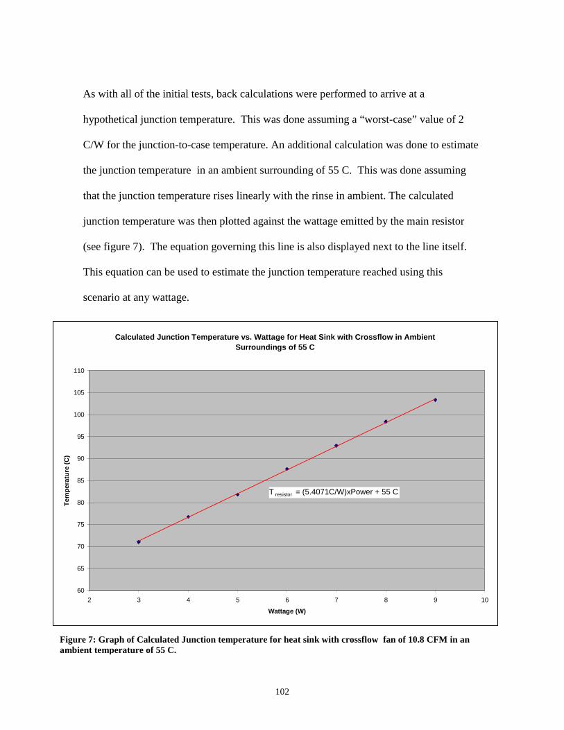
102

As with all of the initial tests, back calculations were performed to arrive at a

hypothetical junction temperature. This was done assuming a “worst-case” value of 2

C/W for the junction-to-case temperature. An additional calculation was done to estimate

the junction temperature in an ambient surrounding of 55 C. This was done assuming

that the junction temperature rises linearly with the rinse in ambient. The calculated

junction temperature was then plotted against the wattage emitted by the main resistor

(see figure 7). The equation governing this line is also displayed next to the line itself.

This equation can be used to estimate the junction temperature reached using this

scenario at any wattage.

Figure 7: Graph of Calculated Junction temperature for heat sink with crossflow fan of 10.8 CFM in an ambient temperature of 55 C.

Calculated Junction Temperature vs. Wattage for Heat Sink with Crossflow in Ambient Surroundings of 55 C

T resistor = (5.4071C/W)xPower + 55 C

60

65

70

75

80

85

90

95

100

105

110

2 3 4 5 6 7 8 9 10

Wattage (W)

Tem

per

atu

re (

C)

103

Heat Pipe with Heat Sink and Fan at Higher CFHeat Pipe with Heat Sink and Fan at Higher CFHeat Pipe with Heat Sink and Fan at Higher CFHeat Pipe with Heat Sink and Fan at Higher CFMMMM A test similar to the heat pipe with impingement fan discussed in the follow up

testing section of the initial report was performed. However, this test differed in two

ways. First, the fan with a higher CFM was used. To allow for fresh air to be blown onto

the sink, a square section just above the fan was cut out of the enclosure top. This was

necessary due to the fact that the impingement fan, being larger than the fan previously

used butted up against the ceiling of the enclosure. This allowed for no head space. Since

it is undesirable to have openings on top of the actual DAQPad, the team felt that the

results of the test would closely resemble a setup with the fan positioned perpendicular to

the enclosure top and partially extended out of the box. To do this, a square section large

enough for the fan to fit through would need to be cut out of the back panel of the box.

To concentrate all cooling of the resistor on the heat pipe alone, the area of the

box containing the circuit boards was completely sealed off with duct tape. This

prevented airflow from the impingement fan from cooling the resistors. The front vents

on the box were also sealed to prevent fresh air from cooling the resistors Utilizing this

scheme, the resistor temperature was maintained at 52 C (while emitting 10 watts). . This

scenario was also tested at 11,12,and 13 watts to arrive at a relation between the

attainable resistor temperature and wattage emitted by the resistor. Temperature readings

were recorded at each wattage until the resistor reached a thermal equilibrium. The

steady state temperatures attained were then plotted against the corresponding wattage to

achieve the plot shown in figure 8. Since the relationship is, again linear, the equation

governing it can be used to determine the temperature attainable at any wattage.

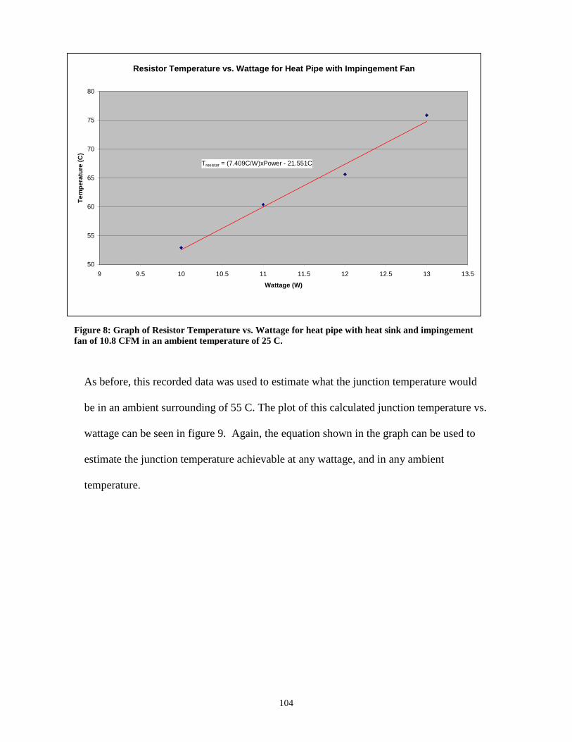
104

As before, this recorded data was used to estimate what the junction temperature would

be in an ambient surrounding of 55 C. The plot of this calculated junction temperature vs.

wattage can be seen in figure 9. Again, the equation shown in the graph can be used to

estimate the junction temperature achievable at any wattage, and in any ambient

temperature.

Figure 8: Graph of Resistor Temperature vs. Wattage for heat pipe with heat sink and impingement fan of 10.8 CFM in an ambient temperature of 25 C.

Resistor Temperature vs. Wattage for Heat Pipe with Impingement Fan

Tresistor = (7.409C/W)xPower - 21.551C

50

55

60

65

70

75

80

9 9.5 10 10.5 11 11.5 12 12.5 13 13.5

Wattage (W)

Tem

per

atu

re (

C)

105

Conclusion

After conducting the experiments discussed in this report in conjunction with those previously

performed, the team arrived at a modified assignment of cooling scenarios for various wattages. These

scenarios include a heat sink, a heat sink with crossflow, a heat pipe with natural convection, and a heat

pipe with impingement airflow. It should be noted that experimentation with these scenarios at varying

wattages resulted in a linear relationship between power dissipated and resistor temperature. The estimated

junction temperature versus wattage plots produced by the team were also linear. These linear relationships

can be used to determine the estimated junction temperature attainable at any wattage. These linear

relationships were expressed using the following relation:

where T = experimental temperature measurement of the resistor before back-calculating for the actual resistor temperature

Figure 9: Graph of Calculated Junction Temperature vs. Wattage for heat pipe with heat sink and impingement fan of 10.8 CFM in an ambient temperature of 55 C.

Calculated Junction Temperature vs. Wattage for Heat Pipe with Impingement Fan in Ambient Surroundings of 55 C

T resistor = (9.409C/W)xPower + 11.898 C

100

105

110

115

120

125

130

135

140

9 9.5 10 10.5 11 11.5 12 12.5 13 13.5

Wattage (W)

Tem

per

atu

re (

C)

106

θeffective = the effective resistance of the scenario from the resistor to the outside air.

P = power emitted by the resistor (chip) Tambient = ambient temperature of the exterior

Surroundings

The team decided upon which of their cooling method scenarios they would suggest for use in the DAQPad

at various wattages based upon the effective resistances associated with each scenario. The lower the

resistance of the system for each scenario that the team calculated, the lower the temperature that the

junction of the actual DAQ would be able to attain. A comparison of the effective resistances for each

scenario can be observed in the bar graph seen in figure 1.

In addition, the team created the following graph in figure 2 to illustrate the maximum wattage

that the chip could emit while remaining at or below 110 oC.

Additionally, the reader should note that proper ventilation would need to be utilized in an actual

DAQ product in order to duplicate the temperature results associated with the heat sink noted in this paper

above. Contrarily, ventilation would not need to be incorporated in an enclosure design that utilized the

heat pipe device, because the large heat transfer capabilities of the heat pipe required little to no ventilation

in order to function. This lack of ventilation was a conservative or worst-case scenario.

Documents

The Design of DAQ Circuit Board Processor Cooling Methods