Embed Size (px)
Citation preview

LEVELTHE DESIGN AND ANALYSIS OF TURBOMACHINERY IN ANINCOMPRESSIBLE, STEADY FLOW USING THE STREAMLINE
l CURVATURE METHOD
Mark W. McBride
Technical MemorandumFile No. TM 79-33February 13, 1979Contract No. N00024-79-C-6043
Copy No.
CI-
CD,
LUl
L~A-... The Pennsylvania State UniversityAPPLIED RESEARCH LABORATORY
C-2 Post Office Box 30
~. _State College, Pa. 16801D
Approved for Public Release EDistribution Unlimited D-•- U )
NAVY DEPARTMENT
NAVAL SEA SYSTEMS COMMAND
,• • . . • -, 1,
UNCLASSIFIED
SECURITY CLASSIFICATION OF T4IS PAGE (When Date Entered)
REPORT DOCUMENTATION PAGE READ INSTRUCTIONSBEFORE COMPLETING FORW
t, REPORT NUMBER 2. GOVT ACCESSION NO. RECIPIENT°S CATALOG NUMBER
TM 79-33 /
C4.j, HEPESIGN AND VALYSIS OF &RBOMACHINERY INý AN Technical 0XamLand'a 1 1r 0
U•( ORESSIBLE, _•TEADY FLOW USING THE STREAMLINE eURVATURE LTHOD P
S. CONTRACT OR GRANT NUMBEROa)
l Mark W. McBride /' 0024-79-C-6043
9. PERFORMING ORGANIZATION NAME AND ADDRESS 10. PROGRAM ELEMENT. PROJECT. TASK
Applied Research Laboratory AREA 4. WORK 9FtLti.UAM!tERS IPost Office Box 30a a y , b '7]7State College, PA 16801
1I. CONTROLLING OFFICE NAME AND ADDRESS 12. REPORT DATE
Naval Sea Systems Command, Code 0351, Washington, February 13, 1979DC 20362 and Naval Ocean Systems Command, 13 NUMBER OF PAGES
San Diego, CA 92152 16114. MONITORING AGENCY NAME & ADDRESS(Il dillfrent from Controlling Olfie) 1S. SECURITY CLASS (of thile rport)
UNCLASSIFIED
15.. DECLASSVl~CATi3N 7 ~wwN5RAOi4GSCHEDULE
IS. OISTRIBU'r'ON STATEMENT (of this Report)
Approved for public release. Distribution unlimited.Per NAVSEA - March 30, 1979
I7 DIST R!".j9fLK &TATk&M&MT (4J te 4s, anLgred in Block 20, It different from Report)
I()ARLPSU/IN..79..331I SUPPLEMENTARY NOTES
IS KEY WORDS (Continue on reverse side it necessary and identity by block number)
turbomachinery
streamline"hydrodynamicscurvature
20 ABSTRACT (Conttnue on reverse aide if neocosary mnd identifv by block i.,bar)
The design of new and more efficient turboulachinery requires an improvedunderstanding of the fluid flow phenomena associated with the duct and bladingrequired for the operation of such devices:, In recent years, the digitalcomputer has made possible the solution of equations of motion pertinent tothis field:'ýie)hstudy described heretdeals vith the design and analysis ofturbomachinery in an incompressible, steady flow, such as hydraulic pumps
DD 1473 COITION OF I NOV O5 IS OBSOLETEjD 1AN EU UNCLASSIFIEDEC RT CL SIIC TO OF '' °< ' THS'AG'(thn ai 'te

UNCLASSIFIED
SECURITY CLASSIFICATION OF THIS PAGE(Whon Dot& Enter.d)
and turbines. The basic numerical approach (*tkaedin the analysis ofthese devices is the Streamline Curvature Method.
~hg.velopment of a turbomachine design method requires an accurate modelof the through-flow describing the spatial variation of the velocity andpressure in the fluid. Equations of motion are developed in a way that allows-i4 modeling of the blade row spanwise and chordwise loading distributions ona blade row and determination of their effect on the through-flow. Theequations are solved using the Streamline Curvature Method with fheý"effects ofviscosity and turbulence included in an empirical fashion due to the complexityof the governing equations. N
Once the turbomachine performance and the subsequent through-flow solu-tions have been determined, the airfoil-shaped blades must be specified toproduce the prescribed flow field. An empirical method of designing airfoilshas been developed by G. F. Wislicenus. this method, the Mean StreamlineMethod, relies on correlations of performance data of blades tested as two-dimensional cascades to construct a blade camber line using the theoreticalmean flow streamline and an offset distribution. The offset distribution isdependent on a number of geometric and flow variables. An analysis was per-formed to extend the range of applicability of the Mean Streamline Method ona new correlation developed to aid in the design of airfoil sections.
Further improvement of turbomachine performance and the development of arational three-dimensional solution of a turbomachine through-flow requires ananalytical approach to blade section design. A Streamline Curvature Methodwas developed to solve the indirect or design problem for blades in a cascade.The properties of the flow at the blade row inlet and exit are specified alongwith the loading distribution along the blade chord that is desired. Ablade-to-blade analysis is performed that satisfies the equations of motionand iteratively determines an airfoil shape that will perform as specified.The effects of the blade surface boundary layers on the flow are included inan empirical fashion. A res4lt of this procedure is a blade-to-blade flowsolution that can be used to construct a three-dimensional representation of
the velocity and pressure fields in the turbomachine.
L Experimental investigations were performed to validate each of the
analysis and design methods described. In general, % performance ofthe various test articles was in agreement with predictions. It isapparent, however, that phenomena associated with turbulent and viscousflows require more sophisticated modeling than those used in this study.
Aurcssiou
1 ificatioLo
DIstribut on/iltbillty Codes I
:Availand/or.• speclal
UNCLASSIFIED
SECURITY CLASSIFICATION OF TWIS PAGE(Whon Pat*a Entredl

liii
ABSTRACT
The design of new and more efficient turbomachinery requires an
improved understanding of the fluid flow phenomena associated with the
duct and blading required for the operation of such devices. In recent
years, the digital computer has made possible the solution of equations
of motion pertinent to this field. The study described here deals with
the design and analysis of turbomachinery in an incompressible, steady
flow, such as hydraulic pumps and turbines. The basic numerical approach
utiliz,:d in the analysis of these devices is the Streamline Curvature
Method.
The development of a turbomachine design method requires an accurate
model of the through-flow describing the spatial variation of the
velocity and pressure in the fluid. Equations of motion are developed ini
a way that allows the modeling of the blade row spanwise and chordwise
loading distributions on a blade row and determination of their effect on
the through-flow. The equations are solved using the Streamline
Curvature Method with the effects of viscosity and turbulence included in
an empirical fashion due to the complexity of the governing equations.
Once the turbomachine performance and the subsequent through-flow
solutions have been determined, the airfoil-shaped -lades must be speci-
fied to produce the prescribed flow field. An empirical method of
designing airfoils has been developed by C. F. Wislicenus. This method,K the Mean Streamline Method, relies on correlations of performance data of
blades tested as two-dimensional cascades to construct a blade camber1' line using the theoretical mean flow streamline and an offset

iv
distribution. The offset distribution is dependent on a number of
geometric and flow variables. An analysis was performed to extend the
range of applicability of the Mean Streamline Method on a new correla-
tion developed to aid in the design of airfoil section
Further improvement of turbomachine performance and the development
of a rational three-dimensional solution of a turbomachine through-flow
requires an analytical approach to blade section design. A Streamline
Curvature Method was developed to solve the indirect or design problem
for blades in a cascade. The properties of the flow at the blade row
inlet and exit are specified along with the loading distribution along
the blade chord that is desired. A blade-to-blade analysis is performed
that satisfies the equations of motion and iteratively determines an
airfoil shape that will perform as specified. The effects of the blade
surface boundary layers on the flow are included in an empirical fashion.
A result of this procedure is a bJade-to-blade flow solution that can be
used to construct a three-dimensional representation of the velocity and
pressure fields in the turbomachine.
Experimental investigations were performed to validate each of the
analysis and design methods described. In general, the performance of
the various test articles was in agreement with predictions. It is
apparent, however, that phenomena associated with turbulent and viscous
flows require more sophisticated modeling than those used in this study.
I

v
TABLE OF CONTENTS
P'age
ABSTRACT ................. ......................... . ..... ii
LIST OF FIGURES ................ .................... ....... vii
NOMENCLATURE ............................ ...................... xii
ACKNOWLEDGEMENTS ............. ..................... ....... xv
I. A GENERAL STATEMENT OF THE PROBLEM AND ITS SOLUTION . . 1
II. STATE OF THE ART ..................... 7
III. ANALYSIS AND DESIGN TECHNIQUE ....... .............. ... 14
IV. THE STREAMLINE CURVATURE METHOD OF THROUGH-FLOW ANALYSIS . 17
4.1 Development of the Equations of Motion ....... ... 18
4.2 The Effects of Blade Rows ..... .............. .. 27
4.3 The Effects of Viscosity and Turoulence ......... ... 31
4.4 Use of the Streamline Curvature Method ...... ... 32
V. THE CORRELATIONAL MEAN STREAMLINE METHOD .. ......... ... 37
5.1 Introduction ............ ................... ... 38
5.2 The Computerized Analysis of Cascade Data ...... ... 39
5.3 Evaluation of the Cascade Data ... .......... ... 43
5.4 Computation of the Offset Distribution ....... ... 51
5.5 Numerical Description of the Oftset Distribution 52
5.6 Estimation of the Blade Pressure Distribution ... 55
q 5.7 Summary .................... ...................... 57
VI. AXIAL FLOW PUMP DESIGN EXAMPLE ...... ............ ... 58
I
vi
Page
6.2 Detailed Blade Section Design .... ........... .... 66
6.3 Axial Flow Pump Tests ..... ................ .... 66
6.4 Test Procedure ........... .................. ... 70
6.5 Test Results ........... ................... ... 73
6.6 Summary ............ ....................... .... 73
VII. CASCADE BLADE SECTION DESIGN USING THE STREAMLINECURVATURE METHOD--GENERAL STATEMENT .... ............... 79
VIII. CASCADE BLADE SECTION DESIGN USING THE STREAMLINE
CURVATURE METHOD--THE NUMERICAL METHOD ... .......... ... 85
8.1 Development of the Numerical Method ... ....... .... 85
8.2 Definition of a Cascade Design Test Case ..... ... 105
8.3 Results of Cascade Airfoil Design Calculations . . 107
IX. EXPERIMENTAL PERFORMANCE VERIFICATION OF THE STREAMLINECURVATURE CASCADE BLADE DESIGN METHOD ........ .......... 109
9.1 Cascade Blade Test Experimental Apparatus ....... ii1
9.2 Comparison of the Analytical and ExperimentalPressure Distribution ...... ................ ... 124
9.3 Comparison of the Analytical and Experimental FlowFields ............... ..................... ... 130
9.4 Summary of the Analytical and ExperimentalComparisons .......... ..................... .... 150
X. SUMMARY, CONCLUSIONS, AND RECOMMENDATIONS FOR FURTHERRESEARCH ........... ..... ........................ ... 152
10.1 Summary and Conclusions ........ ............ ... 152
10.2 Recommendations for Further Research .. ........ ... 156
REFERENCES ............ ................................... .... 159I
t
ip

vii
LIST OF FIGURES
Figure Title Page
1 Sasic Turbomachine Types ........... .............. 2
2 Generalized Velocity Components in an AxisymmetricDuct ............... ............................ 4
3 General Description of Computation Planes in aTurbomachine Blade Row ..... .................. 9
4 General Reference Station Parameters (MeridionalPlane) ............... ........................ ... 19
5 Differential Streamtube Element ..... .......... ... 21
6 Blade Force Components ..... ............... .... 29
7 Detail View of the Streamlines Calculated ThroughTwo Blade Rows ............. .................. ... 33
8 Streamlines in a Francis-Type Turbine . . ............ 34
9 Comparison of Theoretical and Experimental VelocitiesBehind a Blade Row as Solved by the Direct (SpecifiedAngularity) Method ......... .................. ... 36
10 Example of the Output of the Cascade Analysis(Positive Incidence Case) ..... .............. .... 41
11 Example of the Output of the Cascade Analysis(Zero Incidence Case) ....... ................. ... 42
12 Normalized Maximum Offset, AN/C • CL, vs Vane StaggerAngle, 6. . ........... ..................... ..... 45V
13 Normalized Maximum Offset, AN/C • o, vs Vane LiftCoefficient, CLL ............ .................. .... 46
14 Least Squared Error Curve Fit of the NormalizedMaximum Offset, AN/C, vs the Vane Lift Coefficient,CL ................. ......................... .... 48
15 Loa(ing Parameter, Z, vs the Location of the MaximumOffset, C 0.................... .. .................. 50
b ob max
I

viii
Figure Title Page
16 Parameters DefLning the Nondimensionalized OffsetDistribution .............. .................... .. 54
17 General Layout of the Axial Flow Pump Design Example . 61
18 Velocity Profile in Duct Upstream of Rotor ...... .. 62
19 Distribution of Peripheral Velocity at Rotor Exit . . . 63
20 Computed Streamlines for the Axial Flow Pump DesignExample ...................... ....................... 64
21 Computed Blade Row Velocity Profiles .. ........ ... 65
22 Rotor Cylindrical Design Sections ... ........... ... 67
23 Stator Cylindrical Design Sections ... .......... .. 68
24 View of the Axial Flow Pump Rotor and Stator .... 69
25 Overview of the Axial Flow Pump Installed in the Six-Inch Water Tunnel (Flow is from Right to Left) . . . . 71
26 Close-up View of the Axial Flow Pump Rotor and StatorInstalled in the Test Section of the Six-Inch WaterTunnel (Flow is from Left to Right) .... ........ ... 72
27 Experimental and Theoretical Velocity ProfilesImmediately Upstream of the Axial Flow Pump Rotor . . . 74
28 Comparison of the Theoretical and Experimental TotalPressure Rise Across the Axial Flow Pump at DesignFlow Rate ............... ..................... .. 75
29 Performance Data for the Axial Flow Pump .. ..... ... 76
30 Major Phenomena Affecting the Work Done by a Cascadeof Blades ............. ................. ....... 80
31 Schematic Representation of Camber Li,- Corrected toAccount for Potential and Real Flow Effects in aCascade .................... ........................ 81
32 Design Boundary Conditions Input to the Two-Dimensional Cascade Design Procedure .. ......... ... 86
33 Initial Solution Geometry Consisting of a Numberof Parallel Mean Streamlines Between Ideal, ZeroThickness Blades .......... ................... ... 88
34 Generalized Cascade Flow Field Geometry .......... ... 91
j

ix
Figure Title Page
35 Geometric and Physical Variables Required for theIntegration of the Momentum Equation .. ......... ... 93
36 Initial Differences Between the One-Dimensional orAveraged Flow and the Results of the ExactIntegration of the Momentum Equation .. ..... ..... 96
37 The Effects of the Gradual Addition of Blade Thicknessto the Analytical Solution ..... .............. .. 99
38 Illustration of Singular Point at Blade Leading Edge . 100
39 Modification of the Stagnation Streamline to Accountfor Boundary Layer Displacement Thickness and theBlade Uake ....... ..................... ........ 103
40 Prescribed Performance Requirements for the DesignCascade Blade Analysis .... ... .......... ...... 106
41 Computer Generated Plot of the Initial and FinalAnalytical Solution for the Cascade Blade TestCase ................... ........................ ... 108
42 Theoretical Streamline Distribution and Blade ShapeDetermined by the Streamline Curvature Blade DesignMethod .... ......... ....................... .... 110
43 Photograph of Cascade Tunnel uith Tst Blades andThree-Hole Probe Mounted ....... ............... ... 112
44 Detail of Airfoil Section Shape and Location ofHoles for Surface Pressure Measurements ........ 113
45 Three-Hole Probe and Cascade Blade Test Geometry . . 115
46 Expanded View of Three-Hole Probe Tip ........... .... 116
47 Three-Hole Probe Calibration in Open Jet Tunnel . . 117
48 Three-Hole Probe Calibration (C vs a) ......... .... 119
49 Three-Hole Probe Calibration (CPt vs a) ........ .... 120
50 Three-Hole Probe Calibration (C vs a) ....... ..... 122P
51 Theoretical Cascade Blade Pressure Distribution fromSthe Streamline Curvature Analysis .... ........... ... 125
52 Theoretical Cascade Blade Pressure Distribution fromthe Douglass-Neumann Potential Flow Analysis ..... 128
I I i I Ii i i i

x
Figure Title Page
53 Experimental Cascade Blade Pressure Distribution . . . 129
54 Experimentally Determined Velocity Field in theTest Cascade ....... ............... ......... 131
55 Comparison of the Theoretical and ExperimentalVelocity Profiles in the Test Cascade ReferenceStation 20 Percent Blade Chcrd Upstream ...... ..... 132
56 Comparison of the Theoretical and ExperimentalVelocity Profiles in the Test Cascade ReferenceStation Coincident with Leading Edge ...... ... 133
57 Comparison of the Theoretical and ExperimentalVelocity Profiles in the Test Cascade ReferenceStation at 10 Percent of the Blade Chord . . ......... 134
58 Comparison of the Theoretical and ExperimentalVelocity Profiles in the Test Cascade ReferenceStation at 20 Percent of the Blade Chord .... ..... 135
59 Comparison of the Theoretical and ExperimentalVelocity Profiles in the Test Cascade ReferenceStation at 30 Percent of the Blade Chord .... ..... 136
60 Comparison of the Theoretical and ExperimentalVelocity Profiles in the Test Cascade ReferenceStation at 40 Percent of the Blade Chord .... ..... 137
61 Comparison of the Theoretical and ExperimentalVelocity Profiles in the Test Cascade ReferenceStation at 50 Percent of the Blade Chord .... ..... 138
62 Comparison of the Theoretical and ExperimentalVelocity Profiles in the Test Cascade ReferenceStation at 60 Percent of the Blade Chord .... ..... 139
63 Comparison of the Theoretical and ExperimentalVelocity Profiles in the Test Cascade ReferenceStation at 70 Percent of the Blade Chord .... ....... 140
64 Comparison of the Theoretical and ExperimentalVelocity Profiles in the Test Cascade ReferenceStation at 80 Percent of the Blade Chord .... ....... 141
65 Comparison of the Theoretical and ExperimentalVelocity Profiles in the Test Cascade ReferenceStation at 90 Percent of the Blade Chord .... ....... 142
4
xi
Eure Title Page
66 Comparison of the Theoretical ard ExperimentalVelocity Profiles in Lhe Test Cz.cade ReferenceStation Coincih'.n, with Trailinp Edge . . . . . ... . 143
6/1 Comparison of the Theoretical ard ExperimentalVelocity Profiles in the Test Cescade ReferenceStation 20 Percent Blade Chord 1>rmstream . . . . . . . 144
68 Comparison of the Theoretical ard ExperimentalVelocity Profiles in the Test C;'vcade ReferenceStation 50 Percen: Blade Chord iownstream . . . .... 145
69 CasLade Turning A gle as a Funct Ion of Blade ChordReynolds Number...... . .. ................ . . . . 148
/0 Experimental Casc ide Blade Press:ure Distributionas a Function of .,lade Chord Reynolds Number ... ..... 149
xii
NOMENCLATURE
Sytpbocl Definition
A, B, C, D, E polynomial coefficients
a, b, c, d, e polynomial coefficients
CL blade lift coefficient
C percent of blade chord, where AN is a maximum0max
C P pressure coefficient
c blade chord length
k streamline curvature - (R I
L integrated total blade force
t percent of blade chord where one-half of total turningoccurs
N revolutions per second
tAN offset or distance between the mean streamline and theblade camber line
n ordinate normal to a streamline
P pressure
AP pressure difference across a blade
R radius
"Rk radius of curvature of a streamline
r ordinate along a radial line
S spacing of two blades in a cascade
8 ordinate parallel to a streamline
t projected length if a blade in the (x) direction
I

xiii
Snyol Definition
U blade peripheral velocity
u velocity component in (x) direction
V velocity
V volume flow rate per unit depth
v velocity component in (r) or (y) direction
x axial coordinate
y radial coordinate
a angle between a streamline and a path of integration
a relative flow angle
a i incidence angle
8 angle betwen a blade force vector and a streamsurface
13 dummy variable of integration
a B stagger angle, angle between the blade chord line andV axial or (x) direction
n axis coincident with a path of integration
o ordinate in peripheral direction
ordinite on n axis
P fluid density
o cascade solidity (S/C)
* angle between a streamline and the (x) direction
Subscript
I uniform upstream or leading edge conditions
uniform downstream or trailing edge conditions
a axial or (x) component
S1 denotes an integration starting point
L tlocal condition
K

xiv
Symbol Definition
m meridional component, parallel to * direction
o denotes an integration end point
S reference static condition
s local static condition
T reference total condition
T blade thickness
t local total cond.Ltion
x component in (x) direction
x partial differential W. R. T. (x)
y component in (y) direction
y partial differential W. R. T. (y)
ps pressure surface
ss suction surface
a function of flow angle
n function of n
0 peripheral component
denotes a property of a streamline coincident with avalue of E on n
denotes a reference condition
I
I
xv
ACKNOWLEDGEMENTS
The author wishes to express his gratitude to the following
institutions and persons who supported the work reported in this thesis.
Direct support for the various works described in this thesis was
furnished by the Naval Sea Systems Command Code 0351. Funding for the
design, fabrication, and testing of the axial flow pump described herein
was furnished by the Naval Oceans Systems Center, San Diego, California.
Dr. Robert E. Henderson and Prof. Walter S. Gearhart provided
inspiration and technical assistance throughout the investigations
reported here, Many members of the staff of the Fluids Engineering
Department contributed technical assistance to these projects. The
author is a full-time member of the staff of the Applied Research
Laboratory of The Pennsylvania State University and is very grateful for
the opportunity to pursue the work reported herein under the support of
the Applied Research Laboratory.
I:L
4 ,Ln.

CHAPTER I
A GENERAL STATEMENT OF THE PROBLEM AND ITS SOLUTION
The problem addressed in this study is the development of a rational
engineering solution to the design of turbomachinery that operate in an
incompressible, steady flow. The types of turbomachines considered
include axial, mixed, and radial flow pumps, fans, and turbines.
Schematic examples of these types of machines are shown in Figure 1. All
turbomachines require rotating rows of airfoil-shaped blades. Geometri-
cally, blade row shapes can be quite complex, and their shape is closely
related to the exact flow field in the turbomachine. The performance of
a turbomachine is defined relative to the amount of fluid passing
through the machine in a given time and the change in energy, or total
pressure, that the fluid experiences. The indirect or design problem is
one of specifying a geometric shape of duct and blading that will deliver
the desired flow parameters either at a single operating point or over a
continuous range of operating conditions. The direct or analysis problem
considers a given blade row shape and determines the operating points of
the machine. Both problems require methods to determine the exact nature
of the flow field in the turbomachine.
A number of additional considerations must be made during a design,
all of which affect both the machine's performance and geometry. These
* considerations include efficiency requirements, constraints due to
cavitation or fluid vaporization in low pressure regions, unsteady flow
effects, two- and three-dimensional effects of viscosity, and
I
t i

2
FLOW R -4\1sIAXIS OF ROTATION
I i I I ,F I/I IfII I l//I
AXIAL-FLOW PUMP OR TURBINE
R - ROTATING BLADE ROWS - STATIONARY BLADE ROW
AXIS OF ROTATION
S MIXED/RADIAL-FLOW PUMP OR TURBINE
Figure 1. Basic Turbomachine Types.
w

3
manufacturing limitations. All of these constraints and effects must be
considered in a sound, analytical design procedute.
The design of a turbomachine can be traced through three basic
phases. The first is the preliminary design phase in which the type of
machine to be employed is determined. Additionally, the size, speed,
and over-all geometry are determined. Since the entire design process
is iterative, the preliminary design parameters and shapes are always
subject to modification. Many aspects of this preliminary design process
are empirical and/or arbitrary and are based on engineering experience,
system or installation limitations, costs, and other factors of which
the designer must be aware. However, to be able to proceed with a
detailed design, a fairly complete conceptual form of the machine must be
generated.
The second phase is the detailed design of the machine duct and
blade shapes. A design that is baseu on the equations of fluid motion
requires the development of a mathematical description or model of the
flow field and the machine geometry. This phase requires computerized
methods to solve the equations of motion while accounting for as many of
the physical properties and boundary conditions as possible. Since the
direct solution of the equations of motion for viscous, turbulent flow is
impossible, it becomes necessary to approximate some of the physics of
the flow. However, the exact solution of the nonviscous or ideal ilow
field with forces due to fluid accelerations, rotation, and nonuniform
flows taken into account is possible. Figure 2 helps to visualize these
various aspects of the flow geometry. The usual app:oach used is to
solve for the inviscid flow field and superimpose the effects of real
fluid flow which are difficult to treat analytically.
; -- -- - - - - - - - - - -- " - -.

4
- OUTER DUCT OR BOUNDARY
PER I PHERALVELOC ITY_ a MER ID IONAL
IVe PLANE
MER IMD IONAL// VELOICITY (Vm M
INNER
BOUNDARY
AXIS OF ROTATION
Figure 2. Generalized Velocity Components in an Axisymmetric Duct.
I • • m

5
The solution must include physical effects peculiar to each type of
machine. Generally, the inflow conditions to the turbomachine will be
nonuniform in velocity and pressure. The chordwise and spanwise loading
or pressure on the blade rows will be nonuniform as is the blockage due
to blade thickness and boundary layer growth. If the flow field is
unbounded, as for a nonducted fan, additiodal boundary conditions are
necessary to perform a flow analysis. The Effects of viscosity in the
blade row passages must be modeled accurately to achieve the design
performance requirements.
The second phase culminates in an actual blade shape design that
will produce the flow field specified by the analysis. Determination of
this shape is difficult as there are a number of boundary conditions that
,t must satisfy, and the performance of a blade row is highly subject to
real flow phenomena which are not easily approached analytically. Again,
a combination of ideal flow theory and empirical corrections are required
to specify a blade row with desired performance.
The third phase is essentially similar to the analysis and blade
design except that the geometry of the system is fixed and it is desired
to determine the effect of a blade row on the flow field. This should
give the same solution as the original analysis at the design point.
However. the results of performance testing and, in particular, measured
velocity and pressure profiles in the vicintty of the blade row may be
used to test the theoretical analysis and design. Where differences are
found, corrections to the mathematical models or to the hardware may be
required.
In summary, the design and analysis of a turbomachine requires an
accurate description of the internal flow field. A numerical simulation

6
of the turbomachine, including the various components of the equations
of motion in either exact or approximate (empirical) form, must be
constructed. This simulation consists of two basic parts, a meridional
plane or through-flow solution and a blade design method that includes
an analytical blade-to-blade flow solution. Each of these solutions
affects the other and must be developed iteratively to produce a consist-
ent model of the flow. Once a model is generated, a check against the
design requirements must be made to assure that no part of it fails the
design requirements. Once complete, the model must be compatible with
mechanical limitations and manufacturing capabilities. An additional
iteration with the design constraints may be necessary to finally arrive
at an acceptable engineering solution to the design of the turbomachine.
JJ

CHAPTER II
STATE OF THE ART
Before the advent of the digital computer, turbomachine design
relied on experience and intuition more than on theoretical analysis.
The inefficiency of early gas turbines pointed to the need to study the
aerodynamics of turbomachines in depth. To accomplish this end, a
succession of analysis techniques have been developed, used, and, in some
cases, discarded as not being accurate enough. A basic understanding of
the flows in the complicated passages and blading was obtained through
experiment and, in many cases, these data were applied directly to design
problems. Historically, the methods that were evolving started as an
analysis of tested hardware and were extended to the design of new
machines. Numerical methods have been developed that aid in the design
of compressible flows in turbines and compressors, though, at present, a
great deal of designer's art is still required. Attention has not been
so great in the area of hydrodynamic turbomachines, such as hydroturbines
and pumps. Improvements in the design of these machines require better
analysis tools to be developed--the purpose of this study.
The equations of motion for a viscous, turbulent, compressible flow
in a turbomachine are impossible to solve even with the help of thE
largest computers. This has required a reduction of their complexity and
the approximation of various terms, particularly with respect to viscos-
ity ard turbulence. These two phenomena are strongly interrelated and
are caused in part by molecular forces associated with the fluid itself.

8
As such, it has been necessary to reduce the complexity of the flow
mathematically by introducing concepts of macroscopic regions for flow
where simplified equations of motion, coupled with models for turbulent
and viscous effects, work with sufficient accuracy. To reduce the
computation requirements, time and spatial averaging of the equations,
coupled with simple models of real fluid effects, make it possible to
obtain engineering data for various types of flows.
In the early 1950's, Wu [I] recognized these problems and formu-
lated a set of equations which had the possibility of a solution. He
broke the problem of che three-dimensional flow into a set of ccapled
two-dimensional solutions. Figure 3 helps to explain Wu's analysis in
which he broke the problem into two planes generally perpendicular to
each other. One, the meridional plane, describes the flow on hub-to-tip
stream surfaces. The other, the blade-to-blade solution, describes the
flow on planes generally parallel to the hub surface of the machine and
perpendicular to the blading. A complete solution by Wu's method would
i equire a number of both parallel meridional a-d parallel blade-to-blade
solutions. The solutions are coupled and must be solved iteratively to
simultaneously satisfy the equations on all of the solution planes.
At the time of formulation of Wu's analysis, computational methods
and machines were not large or fast enough to give a comprehensive solu-
tion. As a result, many approximate methods evolved. Wislicenus [2]
summarized many of the design techniques in use at the time. Most of
these techniques relied heavily on experimental data to be useful. NASA
[31 also compiled detailed design methods and dat,- available for the
design of compressors.

9
MERIDIONAL OR HUB-TO-TIP PLANE
rrf ~BLADE-TO- BLADE
PLANE
Figure 3. General Description of Computation Planes ina Turbomachine Blade Row.

10
Smith [4] rearranged the equations of motion in the meridional
piane to give a time and spatially averaged picture of the flow in a
blade row. At the same time, additional computerized techniques were
developed to solve the through-flow problem. Marsh [5] and Katsanis
( 6] developed a solution (the Matrix Through-Flow Method) where the
Meridional plane was divided into a grid of roughly square blocks. The
equations for the stream function at every grid point were solved by the
finite difference method, an approximation to the actual differential
equations. These solutions are all basically inviscid and nonturbulent.
Novak [7] formulated a solution (the Streamline Curvature Method) that
solved for the velocities and streamlines rather than the stream
functions. Again, the solution was basically inviscid and nonturbulent.
The problem of losses due to viscosity and turbulence was addressed by
Bosman and Marsh [8], but. in general, experimental data are always
required to adequately model the real fluid effects encountered in a
turbomachine. Davis and Millar [9] made comparisons of the usefulness
* of the Matrix Through-Flow and the Streamline Curvature Methods of
through-flow predictions. They arrived at several conclusions which are
important in the selection of a method for various problem types.
Computationally, both methods require approximately the same amount of
computer time. However, due to very large matrix operations involved, a
much larger computer memory is required for the Matrix Through-Flow
Method.
The Streamline Curvature Mezhod offers an advantage in that the
equations and solution are in terms of physical variables of velocity
and pressure rather than those of a stream function. Additionally,
viscous and turbulence effects are much easier to incorporate into the

11
Streamline Curvature Method because their models are developed in terms
of physical variables.
* A Streamline Curvature Method specifically designed for hydro-
dynamic applications is reported in McBride [10]. This analysis is
important because the effects of the chordwise and spanwise loading and
thicknegs distributions in blade rows are included, and specific loss
correlations for various turbomachine types are easily included. The
through-flow analysis is also designed to be linked to a blade element
analysis yield'ng an inviscid solution of the three-dimensional flow in
a turbom~achine. An interesting capability of this analysis method is
its application to the analysis of unbounded turbomachine flows as
reported by Billet [FI]. A feature of the analysis is that a free
streamline through a nonducted blade row tip is calculated. An addi-
tional extension of this Streamline Curvature Method analysis is reported
in Brophy [12], where the analysis was used to form the basis of a design
procedure for radial flow pumps.
Where the three-dimensional nature of the flow field is required,
deteminL~tion of the effects of the blading on the meridional flow
requires flow field solutions on the blade-to-blade surfaces. The design
of blade sections also requires an accurate analysis technique. Katsanis
[13] was one o•f the tirst to successfully compute the velocity and
pressure di.tribution on the blade-to-blade plane. He used a method
very similar to the Matrix 1hrough-Flow Method. Wilkenson [14] z .pted
"the Streamline Curvature Method to the analysis of blade-to-blade flows.
Thompson [15) used the finite element method, similar to the finite dif-
ference method, to analyze the flow field. None ef these methods was
h

12
adapted to the design problem; all were used fo:. analysis of existing
geometries.
Wislicenus [2] developed the Mean Streamline Method of blade
section design. This method is based on experimental correlations of
fluid turning and the blade pressure distribution. A relationship
between the average or mean streamline on the blade-to-blade surface and
the blade section camber line was developed. Reference of this approach
is reported in McBride [16], where two-dimensional cascade data were
analyzed parametrically and the design method revised based on the
acquired correlational data.
None of the above methods incorporates sufficient modeling of the
turbulent boundary layer flow associated with turbomachine blade rows.
Raj and Lakshminarayana [17] conducted experiments which gave insight
into the nature of the blade boundary layers and the structure of the
wake shed from the trailing edge of a blade. These data will help in the
formulation of more accurate models of this flow phenomenon.
The availability of the various through-flow and blade-to-blade
solutions leads to the possibility of synthesizing a three-dimensional
model of the turbomachine flow field. The interaction of the flow on the
meridional plane and on the blade-to-blade planes becomes important in
this case. The result of blade-to-blade analysis is that forces due to
the geometry of the blading may be determined. Smith and Yeh [18] and
Lewis and Hill [19] formulated analys ,: which predict the effect of
these forces on the through-flow. Howells and Lakshminarayana [20]
obtained experimental data regarding the effects of these body forces on
the through-flow in a turbomachine. Katsanis and McNally [21] and
4 iKatsanis [22] used the Matrix Through-Flow Method as the basis of
I''

13
estimating the three-dimensional velocity field in blade rows. Novak
and Hearsey [23] utilized the Streamline Curvature Method in a similar
manner to generate a quasi-three-dimensional analysis. It should be
stressed that the above techniques are for analysis of already designed
blade rows and do not apply to the actual determination of a blade shape,
i.e., the design problem. This paper will address the design problem by
using the Streamline Curvature Method to construct an averaged through-
flow picture that satisfies the general design requirements. Then two
methods, the Mean Streamline Method and the Streamline Curvature Method,
will be used to actually define blading that generates the flow field
prescribed by the through-flow analysis. Combining the through-flow
analysis and the blade-to-blade analysis, a quasi-three-dimensional
analytical representation of the flow field is generated.
:1
I

CHAPTER III
ANALYSIS AND DESIGN TECHNIQUE
The fundamental problem in the design of a turbomachine is the
specification of a blade row that produces a desired energy or total
pressure change with a given fluid flow rate. Due to possible restric..
tions on the size, efficiency, operating characteristics, and cost of
the turbomachine, additional constraints on the size, speed, and type of
blade row may be necessary. The problem the designer faces is the
optimization of the blade row with respect to these constraints while
still achieving the desired over-all performance.
The design of a turbomachine blade row is accomplished in several
fairly distinct but interactive phases. As progress from one step to the
next is made, the possibility of iterations and back steps is always at
hand if it becomes obvious that some portion of the design will not fit
the performance specifications.
With the specification of the performance parameters and design
constraints, the first phase, the preliminary design, is started. In
this step, the over-all design and dimensions of the blade row are deter-
mined. The performance specifications will determine if axial, mixed, or
radial flow blading is required. The basic blade row sizes and speed
will be determined, and a preliminary layout of the duct geometry is
made.
At this point, the second phase, which is the detailed specifica-
tion of the blade spanwise loading distribution, is performed. Empirical
15
data place limits on the amount of work a single blade row can perform
without severely affecting the blade's efficiency by causing stall or
flow separation. An iteration with the initial design phase may be
necessary to assure that the blade row will not be overloaded and perform
poorly.
The third phase of the design is the development of an axisymmetric,
numerical model of the flow through the duct and blade row. Here,
consideration is made of the exact inflow conditions to the blade row.
The Streamline Curvature Method of through-flow analysis reported in a
later chapter is used to develop the numerical model, solving the
inviscid equations of motion for the flow and correcting the solution for
the flow losses due to viscosity and turbulence that are expected. The
detailed velocity and pressure fields are calculated, and by examination
of these and the power requirements, corrections can be made either to
the preliminary design, if necessary, or to the spanwise loading distri-
bution. The result of this phase is a two-dimensional model of the
turbomachine that satisfies all of the design restraints and requirements
and the laws of fluid motion.
The final phase in the design is the specification of an actual
blade geometry that will give the flow field specified by the through-
flow analysis. This is the most difficult phase of the design problem as
the real fluid effects of viscosity and turbulence play a very important
role in the actual performance of the blade row. The real flow is highly
three-dimensional in a rotating blade row, but because of the complexity
of the flows, the best models that can be used in the design are
two-dimensional. Two methods of specifying the blade geometry are
reported in later chapters.

16
The first method is the Mean Streamline Method, which is basically
empirical and relies on correlation data developed from two-dimensional
tests of blade sections. The second is the Streamline Curvature Method,
which is basically theoretical but relies on correlational data to
calculate the viscosity and turbulence effects. The Streamline Curvature
Method, while specifying the blade shape, also calculates the flow field
around the blade sections.
With the blade geometry in hand, examination of the flow field may
reveal areas prone to separation or cavitation, indicating that adjust-
ments must be made in the earlier phases of the design process. The
final acceptance of the design is then based on the mechanical strength
of the blade and on its suitability for manufacture. Again, additional
iterations, going as far back as the preliminary design, may be nre
sary.
An additional input to the design process is the actual tested
performance of another turbomachine blade row designed by the process.
The Streamline Curvature Method of through-flow analysis may take
measured data and reconstruct numerically the measured flow field.
Comparison with the design data helps to improve the quality of the
necessary correlational data used in the design process, both in the
through-flow analysis and in the blade section design process. This
final iteration is necessary to strengthen the design process and to
improve understanding of the highly complex nature of turbomachine flows.
Ii

CHAPTER IV
THE STRFAMLINE CURVATURE METHOD OF THROUGH-FLOW ANALYSIS
The Streamline Curvature Method refers to a solution technique for
determining the flow on the meridional plane of a turbomachine (the
through-flow prcblem) or on the blade-to-blade planes of the turbo-
machine. The method relies on the ability to define accurately the
streamlines on the meridional plane as shown in Figure 3 and to subse-
quently determine the convective and streamwise normal fluid
accelerations based on their geometry. The Streamline Curvature Method
has been used successfully for the determination of the through-flow
solution for axia•l flow pumps, compressors, and turbines, utilizing
equations of motion written in orthogonal or intrinsic coordinate
systems. Approximations are often made that limit the accuracy of the
analysis, particularly with regard to the influence of blade rows on the
K through-flow. Blade rows have been treated as thick actuator disks with
the effects of chordwise loading, solid blockage, and body forces
internal to the blade row ignored. This chapter serves to document a
Streamline Curvature analysis that addresses the problems described.
Improvement of the SCM requires that the equations of motion used
in the solution be written such that reference stations in the turbo-
machine take arbitrary paths through the machine. This allows the
modeling of the blade row loading distribution. Blade-to-blade effects
may be included as circumferentially-averaged body forces. The equations
are genera. enough that axial, mixed, and radial flows may be calculated.
I,
____ ____ ____

18
Proper choice of the boundary conditions allows both the indirect
(design) case and the direct (analysis) problem to be calculated.
The analysis has been used to design axial and radial flow pumps
and has performed the direct analysis of a nonducted rotor in an infinite
medium, all with good success. Some examples of the use of this analysis
will be presented at the conclusion of this chapter.
4.1 Development of the Equations of Motion
In the axisymmetric inviscid analysis, Euler's equations of motion
are written in a radial equilibrium equation that forms the essence of
the Streamline Curvature Method. The additional equations used are those
which express the conservation of mass: total energy, or pressure, and
angular momentum. The method of solution of these equations requires
that they be solved by successive approximations with the necessary data
taken from the iteratively determined velocity field and streamline
pattern.
Let x and y be tectangular coordinates in a meridional plane,
Figure 3, as illustrated in Figure 4. Euler's equations in these rec-
tangular coordinates for an axisymmetric, steady, incompressible flow
are
av av l aPu T + v T p - yax ay pa
and (4.1)
3u D4 1 aPu -+ v = l
ax ay P dx

19
170
REFERENCE LINE(PATH OF INTEGRATION)
t'--- X
AXIS OF ROTATION
Figure 4. General Reference Station Parameters (MeridionalPlane).
t1

20
Figures 4 and 5 represent the meridional plane of the solution, and
geometric quantities used in the following equations are shown on these
"figures.
The pressure gradient between points a and b, Figure 5, can be
represented by
b b b
aP =p• as +---- (4.2)an as n an (42
a a a
To compute the pressure gradient along n requires the partial
derivatives in Equation (4.2) to be determined.
in the streamwise direction, one has
-P = -p sin ý +2cos (Pas ay ax
Comhining Equations (4.1) and (4.3), we have
1P [u = v + v 'v sin r + 2- + v cos • (4.4)P T ax ay j ax a
Note that
v V sin 0 (4.5)m
and
u V cos
Ii
4. m,

21
Rk / REFERENCE LINE
S.L.
dn d S. L.,
dr
a dAXIS OF ROTATION
Figure 5. Differential Streamtube Element.

2 2
The following derivatives are determined by the chain rule
ax Vm Cos • x+ sin Vmax -m x +m
x
au~ - i + Cos 4Vax ni x in
x
I •_vv V Cos • y+ sin Vm (4.6)
ay m y iY
and
au -V sinp• + cos V3y m Ym
The quantities determined in Equations (4.5) and (4.6) are sub-
stituted into Equation (4.4) and, after reduction, the result is
1 as Vm cos Vm + Vm sin V (4.7)S~y
Equation (4.7) reduces tc
1 3P mp as ms (4.8)
which is seen to be the differentia' form of the steady Bernoulli's
equation for an incompressible flow.,
The streamwise normal component of Equation (4.2) is developed in a
similar manner by noting that
;P- 3 cos 2 - sin • (4.9)
3n - T ax

23
and
1 n 2 + v oCo - 2 + vau sin 4 (4.10)
After combining Equations (4.5), (4.6), and (4.10), we obtain the follow-
ing result:
I aP = 2 Cos + V 2 sin 4 , (4.11)
pTn m x m y
which is equivalent to
1 .V 2 3x ,1 +sy (4.12)IL ~~~an asx sy
The quantity in the brackets in Equation (4.12) is recognized to be
equivalent to a/Ds, the curvature (k) or (Rk)- of the streamline.
Finally, Equation (4.12) becomes
1 aP 2.-. k V .
(4.13)p n
Combining Equations (4.2), (4.9), and (4.10), we determine the radial
equilibrium equation for nonswirling flow to be
ap ap as aP 3nTn -s a aI n + n
and, finally,
k V sin c + V - cosa (4.14)
o aq m mas

24
The pressure gradient due to sw'rl is determined in a similar manner and
leads to the term
1 DP 1 2-p Tr ' (4.15)
where there are no circumfereni~Al derivatives; i.e., the flow is assumed
to be uniform in the circumferential direction. The computational form
of the radial equilibrium is
1•P kV2 sna+1 02 mV
-- kV sin sin(¢+u) + V mcosa . (4.16)m _P oT a m4as
rhe three terms on the right-hand side cr Equation (4.16) represent
the meridional curvature, the radial and the convective accelerations,
respectively. Integration of the equation will yield the static pressure
difference between any two points in the flow field.
From Equation (4.16), the static pressure difference relative to
some point, say ryi, in the flow to another point, F, along the reference
line may be found. To satisfy conservation of mass and energy across the
reference lin!, an absolute value of static pressure must be found at the
reference point, q The foilowing direct solution for this value is an
improvement over other procedures which are iterative in .iature.
A continuity equation may be written for every station in the
problem:-
j) Vm(n) r(n) sin(G ) dn - const (4.17)
ni

25
where ni and n are defined in Figure 4. In words, the mass flow across
a reference line, regardless of its path between two streamlines, is
constant, assuming an incompressible fluid. Bernoulli's equation may be
written along a streamline between a particulp: point, •, on the refer-
ence line and the upstream reference conditions:
1 2 1 2 / 2PP V + PV V8 !P-) dn - pVm .(4.18)
The first two terms on the left-hand side represent the total pressure
(static plus dynamic) available at the point ý. The term P contains
all head loss and rotor energy changes between the upstream reference
condition and the station of interest. The sum of the fourth and fifth
terms is the static pressure at F. The term in the integral is the
static pressure difference between q . and the point , along the reference
line from Equation (4.16).
Equations (4.17) and (4.18) may be combined and integrated between
the two flow boundaries to give
+ - {pV12 - P1 - 1 '• ) d6 r, sin(,,) dn =
!q
V r sin(i d (4.19)
In

26
Because P is a constant, Equation (4.19) may be rearranged to give
ft
no no I 0 2 5 P
2 yo d1ýW Wdr = Poo + •vc - 30) • •Si n n
qin
• }W2dn (4.20)
2 m
where
W r sin (ac) ,
and, finally,
0 1 ~2- 2 1 11 2 d Wdn Pk + LzV -v 0 - 2 V m ) W2 dn
Sni n
n o 2 (4.21)
ni
The static pressure at anj point • along a reference line is then
+ý drP (4.22)
rl qi p

27
The velocity profile which satisfies conservation of angular
momentum and continuity and satisfies Bernoulli's equation along all
streamlines is given by rearranging Equation (4.18).
r • 1/2
V 2 + IP(V V 2 ) P d )rll
The flow field is solved by marching downstream to each station in turn
and integrating Equation (4.16). The static pressure is then obtained
from Equation (4.22). The improved velocity profiles are generated by
Equation (4.23) until the changes in the velocity profiles and streamline
locations are small between two successive passes.
4.2 The Effcct," of Blade Rows
In an inviscid solution of the turbomachine through-flow, the effect
of a blade row is to change the angular momentum distribution in the flow
as it passes the blade row. In the case of a rotating blade row, the
total energy or total pressure of the fluid is changed in a m'anner
proportional to the blade row chordwise loading distribution. In a case
where the spanwise loading or work distribution is not uniform, the total
energy will be changed in a nonuniform way in the spanwise direction as
well. The effect of the blade row is then to change the through-flow
velocity profiles and the streamline pattern.
A rotating blade row ch-ingen the total pressure in proportion to the
change in angular momertum of the fluid passing through the rotor. The
tot,1 pressure is increased between the points I and 2 along a streamline

28
(or, in the case of a turbine, decreased) in an inviscid fluid in
accordance with the equation
AP 21V (4.24)n 2 1
where V is positive in the direction of rotation.
The effect of an airfoil-shaped blade in a flow is to produce a
lifting force perpendicular to the blade surface. For the purpose of
this discusn.ion, it will be assumed that the force can be integrated over
the surface of an airfoil section and concentrated at some point on thr
blade surface. This force can be seen as the force L in Figure 6. The
airfoil cross section of interest lies on the streamsurface that is
defined Uy the axisymmetric through-flow solution. The three components
of the coordinate system are shown as the circumferential direction (0),
the streamwise direction (s), and the streamsurface normal direction (n).
In general, a blade surface is not perpendicular to the streamsurface
defined in the (s, 0) plane, and therefore the lifting forze L will not
lie on this plane. The lift force can be resolved into components along
the axes as shown in Figure 6. The two components of the lift force that
are of principle importance are accounted for by the equations already
discussed; namely, Equation (4.24). These are the circumferential force
L and the streamwise force L . The third force cannot be computed
without foreknowledge of the geometric shape of the blade surface, which
is required in the determination of the angle 6 shown in Figure 6. As
can be inferred from the figure, in the case of blading that is perpen-
dicular to the streamsurfaces, which is true for most radial blade :ows,
the angle 6 is small and the resultant force L normal to then

29
LEE
SSTRE.AM - r
Figure 6. Blade Force Components.
1'
I4 ,

30
streamsurface can be neglected. Occasionally, either due to design or
as a result of the mechanical arrangement of a blade shape, the angle B
can attain significant values and the result of the action of the stream-
surface normal force is to change the through-flow in the blade row,
which in turn affects the blade row performance. When this case is
encountered, an adjustment must be made to the radial equilibrium
equation to account for this force.
The forces shown in Figure 6 are not concentrated but are actually
blade body forces distributed over the entire blade surface. The radial
equilibrium Equation (4.16) requires an additional term where a signifi-
cant body force component perpendicular to the streamsurface is present.
This term is a pressure gradient due to the normal component of the blade
force along the path of integration. Because the path of integiation is
generally perpendicular to the streamsurfaces, the magnitude of the term
is that of the normal blade body force and is usually small.
Calculation of the streamsurface normal body force is difficult
because of its dependence on the geometry of the blading involved. This
implies that a detailed through-flow analysis and blade section design
must be performed before the term can be computed. Additionally, the
force is distributed both in the circumferential direction and along the
streamwise direction. To be properly included in the radial equilibrium
equation, the force must be integrated and averaged in the circumfer-
ential direction to determine its axisymmetric value. Obtaining the data
necessary to generate the term for the radial equilibrium equation
requires determination of the blade-to-blade flow solutions on a number
of streamsurfaces. Once accomplished, the streamsurface normal pressure
gradient along a path of integration within the blade row may be

31
determined by use of finite difference differentiation of the pressures
existing on successive streamsurfaces at constant circumferential
locations. The determined pressure gradients may then be averaged in the
circumferential direction and applied to the radial equiltbrium equation.
4.3 The Effects of Viscosity and Turbulence
Viscosity and turbulence are a result of molecular properties of a
fluid and have profound influences on some regions of a flow. Because of
this, equations describing their effects are extremely difficult to
solve, in particular, where flows have a three-dimensional nature. This
is the case with turbomachinery. The average effect of viscosity and
turbulence on turbomachine flows can be established, however. In
general, a turbomachine flow will experience a total pressure reduction
and a redistribution of velocity as it passes through a duct or blade
row. The magnitude of these effects can be determined experimentally by
acquiring certain data frc testing of a turbomachine. In the case of a
blade row, circumferentially-averaged spanwise (axisymmetric) traverses
of the velocity and pressure field up and downstream of the blade row are
required. By use of the previously described inviscid flow analysis, a
comparison of the tested data and ideal flow characteristics can be made.
This comparison will reveal the magnitude and distribution of the loss in
total pressure that the flow experiences. If a correlation is developed
and applied to the analysis, the result is a model of the real flow
field. In the development of new designs, it must be assumed that the
loss correlations are similar for blade rows of similar characteristics.
32
4.4 Use of the Streamline Curvature M.-thod
To help clarify the nature of the information that can be obtained
from the axisymmetric through-flow analysis described in this chapter,
several examples of calculated flow fields are presented. An actual
design is presented in detail in a later chapter.
The first two examples are indicative of the type of data that must
be generated to begin the detailed design of a blade row. They are the
calculated axisymmetric velocity and pressure fields in the vicinity of
rotating blade rows. In Figure 7 is a plot of the streamline ;attern
around two nonducted blade rows set in an approximately infinite medium.
Both blade rows are adding total pressure to the flow as it passes
through them, and the result is a flow contraction through each in a
manner similar to that calculated by actuator disk theory. The velocity
and pressure field is calculated for each of the reference stations shown
in the figure. The data at the stations corresponding to the blade row
leading and trailing edges are required to begin the detailed design of
blading to produce the calculated flow field.
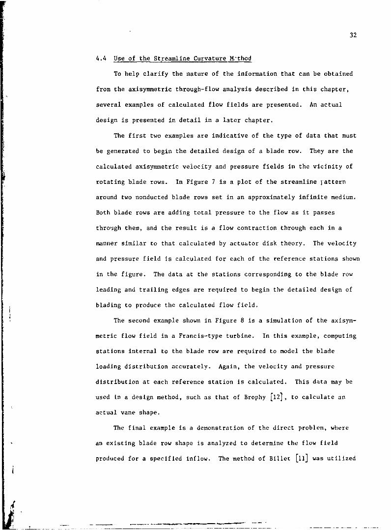
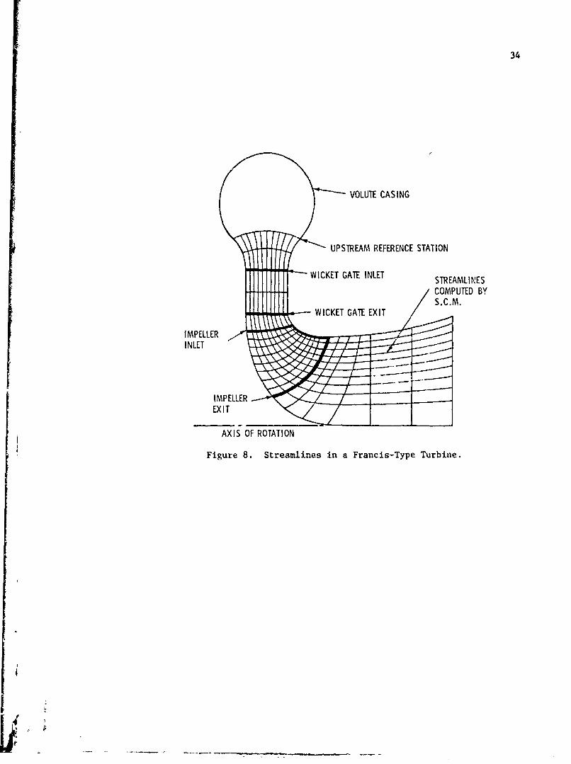
The second example shown in Figure 8 is a simulation of the axisym-
metric flow field in a Francis-type turbine. In this example, computing
stations internal to the blade row are required to model the blade
loading distribution accurately. Again, the velocity and pressure
distribution at each reference station is calculated. This data may be
used in a design method, such as that of Brophy [121, to calculate an
actual vane shape.
The final example is a demonstration of the direct problem, where
an existing blade row shape is analyzed to determine the flow field
produced for a specified inflow. The method of Billet [ii] was utilized

33
BLADE ROW INTRA-BLADEBLADIGEGS STATIONS BLADE ROWLEADING EDGES TRAILING EDGES
COMPUTING•
STATIONS
AXIS OF SYMMETRY
Figure 7. Detail View of the Streamlines CalculatedThrough Two Blade Rows.
f 6*
I
34
VOLUTE CASING
-• U UPSTREAM REFERENCE STATION
SWICKET GATE INLETSTE MI S
COMPUTED BYS. C.M.--- WICKET GATE EXIT
INLET
IMPELLER
AXIS OF ROTATION
Figure 8. Streamlines in a Francis-Type Turbine.

35
to determine the angularity distribution behind a given blade row. The
angularity boundary condition was applied in the Streamline Curvature
Method at the blade row exit plane and the flow field determined
satisfied the flow angularity. Figure 9 is a plot of Lxperimental data
and a comparison with calculated velocities at a blade row exit plane.
'4

36
BLADE R0W EXIT PLANE
MEASURED DATA: Ai 0 Ve N .o/
o AV N /A3a co /
S PREDICTED BY SCM
'-vVco
-r 2 -
001o
zS1- °
0~0 1 1 \_.€ I I I I I I L00 0.2 0.4 0.6 0.8 1.0 1.2
SVELOCITY RATIOS, Ve N0o AND VaNVc
Figure 9. Comparison of Theoretical and ExperimentalVelocities Behind a Blade Row as Solved bythe Direct (Specified Angularity) Method.

CHAPTER V
THE CORRELATIONAL MEAN STREAMLINE METHOD
The Mean Streamline Method of cascade blade section design developed
by Wislicenus [2] correlates the differences in the shape of the blade
camber line and the one-dimensional mean flow streamline. By accounting
for the effects of blade thickness, the boundary layer growth, lift
coefficient, solidity, and loading distribution, blade sections with good
performance have been designed.
Effort has been directed toward the extension of this design method
to cover a wider range of loading distributions, including trailing edge
loaded blades and blades with higher than usual solidities (C/S). A
computer analysis was made of experimental data for many available blade
shapes with differing loading distributions. Relations were determined
for the differences or deviations between the camber line and the mean
flow streamline as a function of the lift coefficient, solidity, a load-
ing distribution parameter, and blade stagger angle.
Using these correlations, a computerized design method was developed
which rapidly produces blade shapes with specified design character-
istics. A radial equilibrium theory is utilized to compute the actual
blade surface pressure distribution. When a blade is to be designed
'hich is similar to existing designs, the method has proven very
reliable.
r

38
5.1 Introduction
The Mean Streamline Method of blade section design due to
Wislicenus [2] is a semi-empirical method of designing a cascade airfoil
section having prescribed fluid turning angle, thickness, and chordwise
loading distribution. The Mean Streamline Method is capable of account-
ing for blade thickness and boundary layer blockage and the effects of
nonuniform pressure and velocity profiles at the blade row inlet and
exit. This design method relies on the ability to determine the depar-
ture of the mean flow streamline from the actual airfoil camber line and
thus, account for the undertu-niag exhibited by blade rows due to viscous.
and potential flow effects. !his departure or offset which is usually
small may be measured experimentally and may be correlated with design
parameters, such as lift coefficient, solidity, loading distribution, and
cascade stagger angle.
The original correlations used in the Mean Streamline Method covered
a rather narrow range of lift coefficient and studied primarily leading
edge loaded configurations. Where cavitation resistance is a primary
consideration, a trailing edge loaded blade is desirable. The trailing
edge 'oaded blade tends to minimize local blade surface velocities near
the leading edge where the static pressure is low. In the present study,
emphasis has been placed on extending the range of this design technique
by correlating a larger range of lift coefficient and data on trailing
edge loaded blades tested by Erwin [24]-
A computer program was developed to analyze available experimental
cascade data. The measured pressure distribution, cascade geometry, and
loading distribution are input to the program. The mean flow streamline
is constructeJ and compared to the camber line tc obtain the offset

39
distribution. The output is in the form of a graphic representation of
the input data and provides the resultant offset distribution and niumeri-
cal results.
The resulting data relating the magnitude and shape of the offset
distribution to the cascade flow parameters were analyzed in several
ways. Direct comparisons were made to the original data of Reference
[2]. Additional correlations were made and, finally, a statistical
method was used to analyze the data. The results indicated that the
offset was more dependent on the lift coefficient and less on the stagger
angle than previously reported. The data also indicate that, in most
cases, extrapolated sections designed using the original data would have
been somewhat over-designed, giving more than the prescribed turning.
This chapter will summarize the computer analysis of the cascade
data and the various correlations derived, and, finally, suggest a
method by which these new data may be utilized in a design Process.
5.2 The Computerized Analysis of Cascade Data
A computerized procedure was devised to quickly analyze the results
of previous cascade testing. The input to this procedure is the blade
geometry and the measured blade static pressure distribution, incidence,
and turning angle. The pressure distribution is prescribed as a function
of the chord and then transformed into a function of projected length in
the axial direction for the purpose of computing the mean flow stream-
line.
The mean streamline is computed by the following procedure. Since
the inlet and exit flow angles are known from the test data, the total
turning is known. Additionally, upstream and downstream axial velocities
I'
~I

40
are assumed constant and continuity is preserved, assuming an incompres-
sible fluid. In the blade passage, blockage due to blade thickness and
the displacement thickness of an assumed boundary layer are used to
extimate the mean axial velocity.
At any given position in the blade passage, the normal velocity
component is computed by the following momentum balance equation:
x
AP dxx
1
Vy(x) t v1 51
APx dx
where the subscripts (x) apply to a given chordwise position along the
blade, (1) applies to that at the blade row inlet, and t is the projected
length of the blade row. Knowing ýhe distribution of both the axial and
normal velocities as a function of the c 4ord position, the mean stream-
line may be computed by using the tangents of the "'low angle at each
axial station. Usually, ten axial stations are used for this purpose.
Once the mean streamline is determined and spline curve fitted, the
offset distr.bution is computed by geometrically comparing the mean
streamline to the blade camber line. The offset distribution is non-
dimensionalized by its maximum value and plotted as in Figures 10 and 11
by a Calcomp 718 flatbed plotter driven by an IBM 1130 computer system.
The mean L-.reamline is also used to compute the mean static pr'essure
line, which is also plotted in Figures 10 and 11. The computation of
this mean static pressure is based on the local mean streamline

41
avoiIN3083d
cr..q^ 0
tnto
0 F
U-0 0w
coo o
0 u0
CooLM.I"00
0o L) CD
-J * Z d 0
C) C) Cxela
'-N

42
avoi0INfl3i3d
LPI
tA 0(AJ
co00c
o '
D iz
#440Q
.0
LonJ
LALJCL CA:0 *q
onI 80 u Li%
-CN
C-4I-
00C
xew NH
43
velocities existing at a given percent of the chord and aesuming that the
total pressure relative to the blade is a constant.
5.3 Evaluation of the Cascade Data
Cascade data from several sources were used in the effort to extend
the range of applicability of the Mean Streamline Method. Two sources
were used to generate the majority of these data, however. The cata
originally used by Wislicenus [2] were used to verify that the computer-
ized procedure yielded the same results that he originally obtained.
These data agree when reduced by the computerized procedure. NACA 65
series data documented in Reference [24] were used to obtain information
over an extended range of lift coefficient for trailing edge loaded
blades. This source documented six pressure distributions at different
angles of attack for each cascade geometry. The zero incidence condition
was found and a pressure distribution interpolated to match this
condition.
Data generated at the Applied Research Laboratory, Reference [25],
were utilized to both verify the computerized procedure and to provide
data points similar to ARL blade designs which often exhibit very high
solidity and use the ARL thickness distribution with the maximum thick-
ness at 60 percent of the chord. Theoretical results of Reference [26]
were used to verify trends and upper limits of camber line offset.
The resulting data relating the magnitude and shape of the camber
line offset distributions to the experimental cascade geometries were
analyzed in several ways. The term AN is defined as the maximummax
measured offset minus the offset at the trailing edge. The quantity
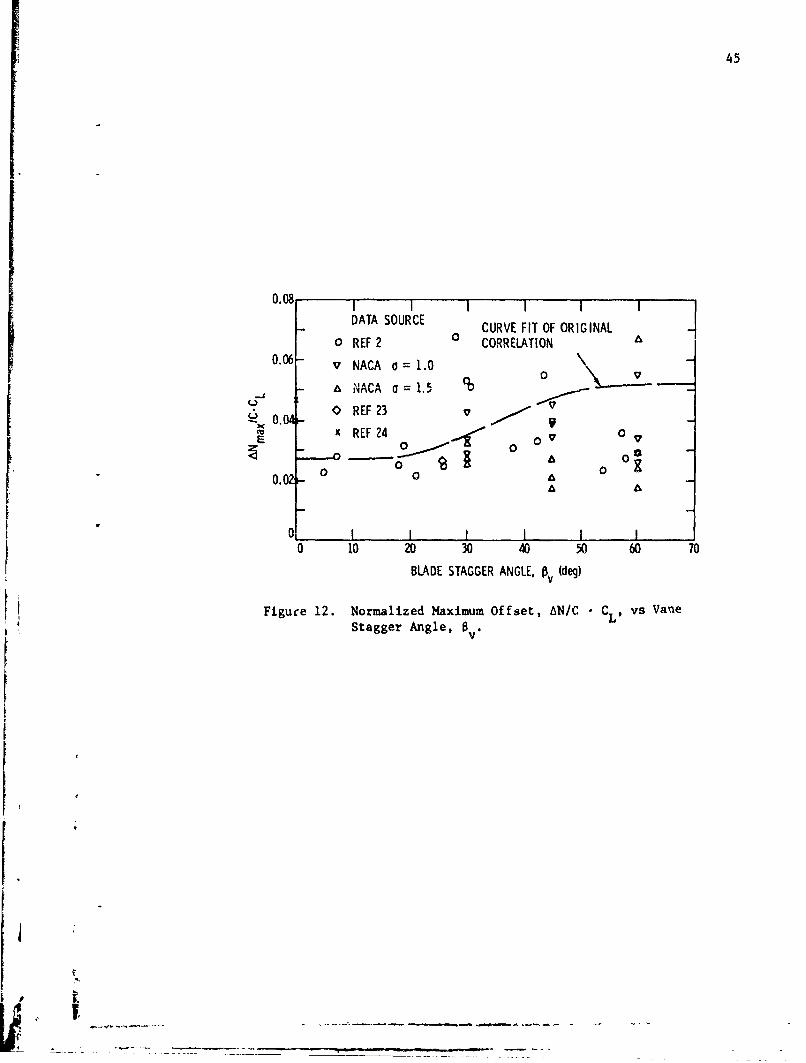
(AN/C max)/CL was plotted against the cascade stagger angle. This is
ma

44
identical to the original correlation of Reference [2]. This plot,
Figure 12, indicates that there is a great deal of variation of the data.
By using the original correlation, a design should be produced that would
generate more than the desired tuiaing in the cascade.
When the qual.tity (AN/C maxCL))a is plotted against the lift coef-
ficient, Figure 13 results. This figure shows a reasonably good correla-
tion with larger offsets associated with the higher lift coefficients.
Theoretical results of Reference [24] fall reasonably close to the
experimental points, and as an upper limit, the isolated airfoil data
line shown also looks reasonable. However, there is still significant
dispersion of the data and only slight correlation with the stagger
angle.
None of the correlations tried yielded definitive results, indica-
ting a much more complex interaction was occurring between four primary
cascade variables. The variables chosen were the lift coefficient (CL),
the solidity (a), a loading parameter (t), and the stagger angle (8y).v
The loading parameter was defined as the percent of blade chord where
one-half of the total turning was accomplished. A high loading
parameter infers that the blade is trailing edge loaded.
A least squared error curve fit was used to determine the nature of
the dependency of the offset on the four cascade variables. A curve fit
of the following form was assumed:
AN c d te 8f (5.2)C + b a c b * a . v (
and a computer program utilizing an iterative technique was used to solve
for the six coefficients while minimizing the total error in predicting
the maximum offset. This error was defined by the relation
t!I . ... .
F 45
0.08IiIIII|
IDATA SOURCE CURVE FIT OF ORIGINAL
0 REF 2 0 CORRELATION
0.06 v NACA O=1.0
a NACA o=1.5 o0REF23 23
"0.04cc X REF 24° 0 0
E
0. 02 0 0
II I I II
10 20 30 40 50 60 70
BLADE STAGGER ANGLE, pv (deg)
Figuce 12. Normalized Maximum Offset, AN/C CL, vs VaneStagger Angle, Bv.
€V
I
[4

46
0.10 I I I I I I I I II
o REF 2
0.08 v NACA ov = 30
SNACA v = 4560
:- NACA v = 600.6- 0 REF 23 x•,/.
x REF 24 X 0 o3Xoo-.F A x 0 0~0.04
00
0.02- A V V V
0 0.2 0.4 0.6 0.8 1.O 1.2 1.4 1.6
LIFT COEFFICIENT, C L
Figure 13. Normalized Maximum Offset, AN/C a o, vs VaneLift Coefficient, C
I
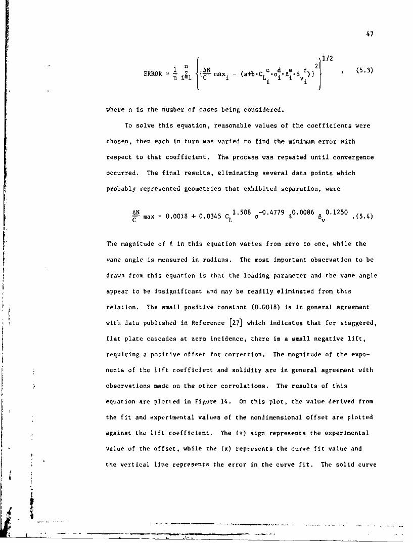
47
1 n 2}1/2
ERROR= 1 1 {•- - cde (5.3)SLi i
where n is the number of cases being considered.
To solve this equation, reasonable values of the coefficients were
chosen, then each in turn was varied to find the minimum error with
respect to that coefficient. The process was repeated until convergence
occurred. The final results, eliminating several data points which
probably represented geometries that exhibited separation, were
AN1.508 -0.4779 0.0086 0.1250-N max 0.0018 + 0.0345 C L 24 . (5.4)
The magnitude of 2 in this equation varies from zero to one, while the
vane angle is measured in radians. The most important observation to be
drawn from this equation is that the loading parameter and the vane angle
appear to be insignificant and may be readily eliminated from this
relation. The small positive constant (0.0018) is in general agreement
with data published in Reference [27] which indicates that for staggered,
flat plate cascades at zero incidence, there is a small negative lift,
requiring a positive offset for correction. The magnitude of the expo-
nents of the lift coefficient and solidity are in general agreement with
observations made on the other correlations. The results of this
equation are plotted in Figure 14. On this plot, the value derived from
the fit and experimental values of the nondimensional offset are plotted
against the lift coefficient. The (+) sign represents the experimental
value of the offset, while the (x) represents the curve fit value and
the vertical line represents the error in the curve fit. The solid curve
4 1

48
0.08-
0.06
X
E
ZZ" 0.04-
I + EXPERIMENT0.02- x CURVE FIT
1+ ANmax/C Z 0.0018 + 0.0345 CL 3/211/2
0. 1.0 0.5 1.0 1.5 2.o 2.5
LIFT COEFFICIENT, CL
Figure 14. Least Squared Error Curve Fit of theNormalized Maximum Offset, AN/C, vsthe Vane Lift Coefficient, CL.

49
represents a curve fit for a condition of unit solidity and a symmetrical
loading distribution. The mean error in (AN/C max) for these data was
less than 0.005, less than 10 percent of the usual offset values used in
a design. Some divergence is seen at higher lift coefficients, which
would be expected due to flow separations.
Finally, a curve fit of the form
AN 3/2//-a = 0.002 + 0.035 C (5,5)
closely approximates the derived curve fit and would lead to slightly
more than the desired turning angle in a dceign process.
The actual shale of the offset distribution varies considerably and
is highly dependent on the incidence angle of the cascade. The NACA
data used specified an incidence of 0 degrees and results in a cusp in
the leading edge of the cascade as seen int figure 11. TVe data of
Wislicenus [2], however, are not specified at the zero incidence condi-
tion and results in an offset distribution similar to Figure 10. Here,
the deviation caused by the offset decreases the effective incidence
angle and should be helpful in reducing the possibility of leading edge
suction face cavitation. The data analysis indicated that the shape of
the offset distribution on the trailing edge side of the maximum point
was fairly consistent, while the shape and magnitude of the leading edge
varied considerably, an observation also made in Reference r21.
In a design exercise, the location of the maximum offset should be
important and prehaps related to the loading distribution shape. Figure
l' was an attempt to make this correlation. The loading parameter is
plotted against the percent chord of the maximum offset. Although there
is considerable dispersion of the data, the straight litie is a reasonable

50
1.I I I I
0.8- o REF2 /v NACA
N 0 REF 23c- 0.6-
=v 0<
0 0.2-
I i I I 1 I I I0.2 0.4 0.6 0.8 1.0
LOCATION OF MAXIMUM OFFSET, C°max
Figure 15. Loading Parameter, Z,, vs the Locationof the Maximum Offset, C
0max
XfX
i
- 4~ - -

51
fit and indicates that the maximum offset is generally toward the
trailing edge and shifts toward the trailing edge as the loading shifts
rearward, again as would be expected.
There is no apparent correlation for the leading edge offset
distribution, leaving the designer relatively free to choose this shape,
either for cavitation resistance or zero incidence.
5.4 Computation of the Offset Distribution
The designer is free to choose the loading distribution to be used
for a particular cascade. This distribution is integrated to determine
the loading parameter, t, which is related to the position of the chord
at which one-half the total work of the blade is accomplished. In more
precise terms,
X-t 2
AP(x)dx = P(x)dx (5.6)
solving for t. This can easily be done graphically c. numerically, or if
a symmetrical loading iz used, the loading parameter is 50 peecent. This
is substituted into the relation
C 0 0.5 + 0.525 • 2 , (5.7)Max
where C is the percent chord at which the maximum offset exists.max
This relation is derived from Figure 15. The lift coefficient (CL) is
known fcom the through-flow analysis and is substituted into the approxi-
mate relation for the maximum offset, along with the solidity, which is
known from the chord length and the blade spacing. Then,

52
C max = 0.002 + 0.035 C L (5.8)
When the computerized Mean Streamline Method of Reference 1281 is used,
the lift coefficient, solidity, and chord length are determined itera-
tively and the above relations for C and AN/Cmax must be used withinmaxthe process.
The shape of the offset distribution is determined as follows. An
incidence at the leading edge is chosen, such as zero, for shock free
entry or more probably a small negative incidence, usually about 1 degree
for cavitation suppression.
The offset distribution must be determined as a continuous, smooth
furction of the chord position. In the computerized design that is
described later in chis chapter, a polynominal curve fit is made to the
necessary boundary conditions. Alternate methods may be used even to
tG,. extent of laying out a distribution using mechanical spline curves.
5.5 Numerical Description of the Offset Distribution
The information generated by the correlation relations is sufficient
to numerically describe an offset distribution. A polynomial may be
generated that satisfies the following boundary conditions:
AN
Y/C(C ) = • maxmax
Y'/C(C ) 0 0.0max
Y/C(100% C) Q 0.0
-I

53
and
Y/C(O.0%) YLE
where (Y/C) is the value of the offset and (Y'/C) is the slope of the
offset distribution. The last parameter is arbitrary and may be adjusted
to prevent reverse camber or obviously undesirable offset shapes from
being determined. Usually, YLE may be set to zero.
A polynomial of the foni;
Y/C = A(x/c)4 + B(x/c)3 + C(x/c)2 + D(x/c) + E (5.9)
will satisfy all of the above boundary conditions. Some design intuition
must be used, especially whea selecting the incidence angle. The quan-
tities used above are shown graphically in Figure 16.
The coefficients may readily be determined:
E YLE
D TAN(al)
AN2 Ca
A (TAN(i)-E 2 3) + YLE( 1 2 0 - £ )/(lC )o C C maxmax o o
max max
AN
B (TAN(ai( 1 ) + YLE( 1Z 1) /(-o )
0 C C maxm•ax 0 0max max
-(I + C )max
and
"- - - - t - .l9*

54
a,
YLE = ANICmaxmax ________ __
Figure 16. Parameters Defining the NondimensionalizedOffset Distribution.

55
C = - (+TAN(a i)+YLE+A+B)
These results are applied directly to the computerized design procedure.
5.6 Estimation of the Blade Pressure Distribution
The design process develops, at a certain percentage of the chord,
the static pressure difference across the blade and the average through-
flow velocity. Additionally, the total pressure of the f'ow is known
from consideration of inlet conditions, the change in angular momentum,
and the rorational speed, if any. An approximate solution for the
surface static pressures may be developed from this information.
The av,!rage total pressure at any point in the blade row may be
expressed as
Pt a Ps + {(Vm +AVmx)2 + (V20 -Ux) (5.10)
This quantity is assumed to be constant across the channel from the
suction to the pressure surface. It is necessary to find the variation
of relative velocity across the channel and at the same time assure that
the volume flow rate is conseived.
The static pressure difference between the suction surface (ss) and
the pressure surface (ps) is known (AP), and the gradient is assumed to
vary a•t the square of the lo;cal velocity. This is equivalent to assuming
that the curvature of the streamlines is uniform across the channel.
Therefore,
1AP = Const cos(y) dy (5.11)
Ss

56
where (y) is the local flow angle and W is the local relative velocity.
The volume flow rate per unit depth may be expressed as
ps
SJW(y) cos(y) dy (5.12)
ss
and, combining the three previous equations,
PS
.2 r 1/22 ts-AP(y)) cos(y) dy , (5.13)
ss
where P is the suction surface static pressure and AP(y) is thess
pressure difference between the suction surface and some point in the
channel. Knowing the distributions of local relative velocity W(y) and
static pressure, the suction surface static pressure may be determined:
Pss JPt - W(y) 2 - AP(y)} dy . (5.14)
Once the suction surface static pressure is known, the velocity and
static pressure gradients may be reevaluated in an iterative procedure
which will converge in about five steps. As an initial guess of the
velocity and pressure distributions, a uniform velocity and linear
pressure are used. In each step of the cycle, the velocity distribution
is checked for volume flow and corrected to match the proper valve.
This method produces a pressure distribution quite similar to the
estima~ton method used in Reference [2] but is slightly less
K

57Iconservative in predicting the minimum pressure, i.e., the minimum
pressure is slightly higher than that found by the method of Wislicenus
[2]
5.7 Summary
A significant range of cascade data was analyzed to provide refined
input to the Mean Streamline Method of blade section design of Reference
[2]. The maximum deviation or offqet of the camber line from the mean
flow streamline has been shown to be primarily a function of the blade
lift coefficient and solidity. The loading distribution and vane stagger
angle are shown to have only a small effect on this deviation. The shape
of the offset distribution is influenced to a degree by the loading
distribution.
A method of computing offset distributions for pumps or subsonic
compressors has been presented that is valid for a wide range of lift
coefficient and loading parameter. In all cases, the offset correction
is small compared to the chord length, and the error in specifying this
offset may be considered insignificant. The shape of the leading edge
of the offset distribution is poorly correlated with any of the blade
parameters, and it is apparent that the designer is free to adjust this
shape for shock free entry or cavitation suppression on the suction
surface as desired.
An approximate method of determining the blade pressure distri-
bution has been presented. The method satisfies the pressuie difference
required by the loading distribution and conservation of mass and total
pressure. The method is based on a simplified radial equilibrium
approach, and it is felt to be more accurate than previous methods of
a~proximation used with the Mean Streamline Method.

CHAPTER VI
AXIAL FLOW PUMP DESIGN EXAMPLE
A simple axial flow pump was designed by the use of the Streamline
Curvature Method and the Mean Streamline Method of blade section design.
The flow geometry was simple enough that a one-dimensional through-flow
analysis would have sufficed, except that, due to blade geometry
problems, a rotor with nonuniform spanaise loading was required. This
in turn causes a radial displacement of the streamlines which in turn
requires the use of a radial equilibrium theory to predict the through-
flow. Because the inflow is a fully developed boundary layer flow, the
Streamline Curvature Method must be used for the solution in lieu of
simpler radial equilibrium approaches.
The design requirements of the axial flow pump are:
Volume flow rate Q 1000 gpm
Head rise H - 36 ft of water
Shaft speed N - 6000 rpm
Rotor tip diameter D t 0.312 ftt
Rotor hub diameter D h 0.12 ft
Casing diameter D = 0.315 ft
Inlet head H - 150 ftsv
4

1: 59The suction specified speed is
S = N(rpm) Q(gpm) = 3829 (6.1)H 3/4
sv
In Reference [29], it is indicated that cavitation inception should not
occur until values of S approaching 6300 are obtained. The head coef-
ficient, *, for the pump rotor is defined as
Z= - 0.121 (6.2)
where Ut is blade speed at the blade tip. In Reference [2], it is shown
that values of p as high as 0.2 can be handled by a single stage axial
flow pump. On the basis of the above, a single stage axial flow pump is
selected.
From Reference [30], the specific speed of the pump indicates a
hydraulic efficiency of approximately 0.80. An estimate of horsepower
required and the shaft torque can now be made, where
Shaft Horsepower - yH Q(cfs) . 11.36 HP550
and
Shaft Torque - Power/20N - 9.94 ft lbs
where N is the rotational speed in revolutions per second.
6.1 Flow Field Calculations Through the Axial Flow Pump
The Streamline Curvature Method of through-f low analysis presented
in an earlier chapter was used to obtain the flow field solution used in
iV

60
the design of the axial flow pump. This technique assumes the flow to
be axisymmetric and requires as input the radial distribution of velocity
and energy at some station upstream of the pump, as well as the radial
distribution of peripheral turning to be placed in the flow by the blade
rows. The meridional velocity at station (1), indicated on Figure 17,
was estimated based on the Blaslus seventh-root law for turbulent flow in
smooth pipes and modified as recommended in Reference [31] to correct for
the higher Reynolds number effects incurred for this particular applica-
tion. The velocity profile is influenced by the presence of a diffuser
and bends located in the pipe upstream of station (1), but there is no
means of predicting their effect. The velocity profiles at station (1),
based on the seventh-root law for boundary layers and also modified for
Reynolds number effect, are shown in Figure 18. The modified profile was
assumed to apply in this design.
The radial forced vortex distribution of peripheral velocity
selected to impart the required energy to the flow is shown by Figure 19.
Also plotted is a distribution for a free vortex radial loading distribu-
tion, and it is apparent that less turning is required near the root
sections if the forced vortex loading is used. The reduced turning near
the blade root is desired to prevent the possibility of flow separation
from the blade surface and to ease manufacturing problems.
The axisymmetric streamline solution derived for the -,imp is shown
in Figure 20. The velocity profiles obtained at the rotor inlet and
exit, as well 3s those at stator inlet and exit, are shown in Figure 21.
The integrated value of head based on a mass average equals 36 feet,
if the peripheral velocity and meridional velocities of Figures 19 and 21
are used.

61
OUTER CASING
FLOW =- 1.89'
TRANSITION ROTOR STATO1.75' SECTION STATOR
S0. 72'
AXIS OF SYMMETRY
Figure 17. General Layout of the Axial Flow PumpDesign Example.

62
20
,.., I-CASING WALL
1.6-""-
LCYPF SEVENTH-ROOT'- LAW
0.4- AT STATION QCORRECTED FOR RREYNOLDS NUMBE
0 0.2 0.4 0.6 0.8 1.0 1.2
MERIDIONAL VELOCITYMEAN AXIAL VELOCITY
Figure 18. Velocity Profile in Duct Upt~tream of Rotor.
J_

63
2.0 • T
"! \ CASING WALL
1.6- FREE
-- ' VORTEXLOADING
1 .4- DISTRIBUTIONz
1.2-
1.< FORCED VORTEX
"o (USED IN DESIGN), 1.0 - LOADING
DISTRIBUTIONUSED FOR DESIGN
0.8 - HUB
0.2 0.4 0.6 0.8 1.0 1.2
PER I PHERAL VELOCITYMEAN AXIAL VELOCITY
Figure 19. Distribution of Peripheral Velocityat Rotor Exit.

64
.• OUTER CASING
S~~STATOR
AXIS OF SYMMETRY
Figure 20. Computed Streamlines for the Axial Flow PumpDesign Example.

65
2.0CASING WALL
1.8 ROTOR INLET
1 ROTOR EXIT • j1z.6 \
"' 1.4
C-
o 1.2-
i- STATOR INLET,-,- 1.0-_ STATOR EXIT 7 .,•_•
0.8 -
0.6-0 0.2 0.4 0.6 0.8 1.0 1.2
MERIDIONAL VELOCITYMEAN AXIAL VELOCITY
Figure 21. Computed Blade Row Velocity Profiles.
I

66
6.2 Detailed Blade Section DesLgnn
The velocity profile data developed by the Streamline Curvature
Method was used as input to the Mean Streamline Method of blade section
design. Cylindrical sections at five equally spaced radii were desig-
nnted for both the rotor and stator. Preliminary considerations of blade
loading were used to determine the projected length of each section to
give a lift coefficient of approximately 0.7. This distribution of blade
length war modified slightly to ease problems of manufacture and the
physical constraints imposed by the duct and resulted in the blade plan-
form depicted in Figure 17. The streamline representing the pump casing
has a theoretical zero velocity. To aid convergence of the Streamline
Curvature Method, the velocity at the wall is given an initial value of
one-half the mass averaged duct velocity. In the design of the blade tip
section, the velocity associated with the streamline 2 percent inside the
casing ia used to represent the tip flow condition.
The developed cylindricrl sections for the rotor and stator are
plotted in Figures 22 and 23, respectively.
Once the blaue section shapea were finalized, the lofting procedure
ot Reference [32] was used to develop rectangular sections for each
blade. The rectangular blade sections are input to a series of computer
programs that produce data necessary to operate o numerically controlled
milling machine with the blade surfaces numerically machined. The fillet
area at the hub is machined by conventional methods. A photograph of the
fi,•ished pump blading is shown by Figure 24.
6.3 Axial How Pu;!L Tests
The axial flow pump was installed in the ARL/PSU six-inch waý.er
tunnel. An adapting collar and nozzle mated the smsllhr diameter rotor

67
TIP
Sj ROTATION
Figure 22. Rotor Cylindrical Design Sections.
4

68
LEO
T I P gnO n
Figure 23. Stator Cylindrical Design Sections.

69
va
, .?>--J
S4J'a
Sr0
-,4
I.~'.-4
1 . . .

70
and stator (3.78 inches) to the six-inch diameter water tunnel test
section. Orifice plates installed in the legs of the water tunnel pro-
vided the necessary pressure drop to test the pump from 50 percent to 150
percent of its design capacity. The water tunnel main drive pump was used
to control the flow rate through the pump.
Surveys of velocity and total pressure just upstream and downstream
of the pump were used to determine the flow rate and total head rise of
the pump. A torque cell was used to determine inpput power to the rotor.
Cavitation performance was noted using the tunnel pressure system, but the
validity of the results is limited due to the &.±ov response of the tunnel
pressure system and the uncontrolled high air content in the water.
6.4 Test Procedure
The axial flow pump was installed in the six-inch water tunnel as
shown in the photographs of Figures 25 and 26. The flow field through the
pump was measured with a wedge probe installed approximately 2 inches
upstream of the rotor and a Kiel total pressure probe installed approxi-
mately 1 Inch downstream of the stator. A four and one-half inch orifice
plate was installed in the downstream vertical leg. A three-inch orifice
plate was installed in the upstream vertical leg.
The upstream wedge prnhed was nulled befoie true readings of total
pressure were made. ihe downstream Kel probe was designed to read total
pressure while eliminating any effccts of rotation in the flow. The data
taken over several tests indicated that over-all the data were repeatable
to within 3 percent.
The upstream and downstream probes were set at 0.7 of the blade span
and a setting of the water tunnel pump was determined that yielded the
correct total pressure rise for the corresponding RPM of the pump. At

71
0 4w
CL
134 4-4
%-4 ~

72
0H
431
00
Q; 0j
0. -44-
W 0l
~0 0

73
these settings, the upstream velocity profile and the downstream total
pressure profile were obtained as a function of radius.
Both profiles were integrated to give the mass-averaged velocity at
the pump inlet and the mass-averaged total pressure at the stage exit.
The upstream velocity probe and the downstream total pressure probe were
set at a radius that corresponded to the mass-averaged values. It was
assumed that the shape of the velocity and total pressure curves did not
change appreciably with flow coefficient and the main tunnel pump was
used to systematically vary the flow coefficient. The average velocity,
average total pressure rise, and shaft torque were recorded for a range
of flow coefficients.
6.5 Test Results
The upstream velocity profile and probe location which corresponds
to the mass-averaged velocity for the rotor are presented in Figure 27.
The total pressure survey data are shown in Figure 28. With the probes
located as shown in Figurew 27 and 28, the total pressure coefficient and
powering requirements obtained are presented in Figure 29. Some care
must be used in interpreting the efficiency curves since very large (40
percent) bearing torque values were measured, decreasing the accuracy of
the powering data.
6.6 Summary
The axial flow pump was tested in the ARL/PSU six-inch water tunnel
from 50 percent to 150 percent of its design capacity. Tests indicated
that the design placed 13 percent too much total pressure rise into the
fluid and, hence, required more power to drive than anticipated.

74
2 TIP______
MEASURED PROFILE
VELOCITY PROBE LOCATION
RADIUS THEORETICAL PROFILE(inches) _ _ _\,"
HUB
0 , . I i I0 0.5 1.0
AXIAL VELOCITY RATIO, Va/VN
Figure 27. Experimental and Theoretical VelocityProfAles Immediately Upstream of the
Axial Flow Pump Rotor.
I

75
I I . .
2 TIP0-m -
THEORETICAL ,/
(KEIL PROBE
LOCATION)(inches) 1 _.
SEXPERIMENTALf HUB
NOND IMNIA ,/1 2 3
NONDIMENSIONAL (P 2pTOTAL PRESSURE RISE -I
Figure 28. Comparison of the Theoretical andExperimental Total Pressure RiseAcross the Axial Flow Pump at DesignFlow Rate.
*

76
0.3--
0.9
0.
ii 0.2- DESIGN 0.7POINT
"-0.6 >:
Ln i
0.5
, 0.1 -L
S\ -0.4
0 I0.3 0.4 0.5
FLOW COEFFICIENT, V.o/Ut
Figure 29, Performance Data for the Axial Flow Pump.

77
Analysis of the results of the axial flow pump design and test
reveals several possible explanations for the differences between the
design specifications and the test results. First, the inlet velocity
profile in the test facility was different than that anticipated for the
design application. Figure 27 reveals this difference. At the tip of
the rotor, the blade incidence was considerably higher than anticipated
and could have contributed to the increased torque and pressure rise
noted. Additionally, the original estimation of the stage efficiency
(n = 0.80) was conservatively low by at least 5 pt'rcent for this parti-
cular application. Because of this low estimate, higher than required
blade loading would be specified. An accurate indication of the actual
rotor efficiency could have been obtained experimentally if velocity
and angularity measurements could have been made between the rotor and
the stator. However. due to the proximity of the two blade rows, a
probe could not be placed in a position adequate for the required
measurements. It is apparent from Figure 28 that the distribution of the
total pressure rise is correct but that a uniform increment has been
added, supporting the argument that the estimated design value of eifi-
ciency was too low. A modification to the trailing edge of the rotor was
necessary to bring the pump t., its design point and also indicated that
too much loading was specified in the preliminary design.
The design point efficiency as derived from powering data in Figure
29 is 0.78. Howevec, considerable error may be present in this figure
due to bearing tare forces of at least 40 percent of the total shaft
torque. This situation was caused by a bearing and shaft requirement for
the test which could not be altered.

78
It is not apparent that these test results support the use of the
design procedures described, although the performance problems seemed to
be a result of the preliminary design rather than the detailed analysis.
Because cf the boundary conditions imposed by the preliminary design, a
simplified through-flow analysis could not have been used. While agree-
ment of the theoretical and experimental flow fields was not as good as
anticipated in this case, other design examples of a more complex nature
have shown excellent agreement as can be seen in Figure 9.
II

CHAPTER VII
CASCADE BLADE SECTION DESIGN USING THE STREAMLINECURVATURE METHOD--GENERAL STATEMENT
An empirical method of satisfying an airfoil section with a
prescribed leading distribution was explained previously. This method,
the Mean Streamline Method, relied on correlational data to correct a
theoretical blade shape based on the mean flow streamline to account for
the effects of potential flow Interactions and viscous losses encountered
in a cascade of blades. The correlations geometrically increase the
camber of the airfoil section in such a way as to compensate for the
underturning experiLnced by the airfoil in actual operation. Figure 30
shows the major causes of cascade blade performance degradation,
In the Mean Streamline Method, all of the geometric and flow effects
are lumped into a single correlation or camber line curvature correction
as shown in Figure 31. A large number of airfoils were found in the
literature which had substantial test data available. New cnrrelations
were developed which separated the major physical parameters in such a
way as to show how each contributed to the design of the airfoi]. The
interesting results of this study were that only section lift coefficient
and cascade solidity had any important effect on the airfoil performance
or on the geometric shape of the theoretical camber line.
The direct theoretical determination of the required blade camber
line is of great practical interest, as the effect of various geometric
and fluid parameters can be determined separately. Additionally,

80
BOUNDARY LAYER ANDSEPARATED FLOWS
-,tm FLOW 'UNDERTURNED'< •DUE TO COMBINED< ,REAL FLOW EFFECTS
CURVATURE DUEW ~TC POTENTIAL ,
ONE-D IMENS IONAL / TURBULENT WAKE
MEAN-FLOW SHED INTO DOWNSTREAM
STREAMLINE FLOW
FigurE 30. Major Phenomena Affecting the Work Done by aCascade of Blades,
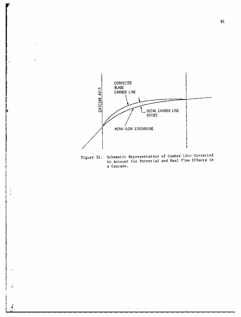
81
CORRECTEDBLADECAMBER LINE
LOCAL CAMBER LINEOFFSET
I L MEAN FLOW STREAMLINE
Figure 31. Schematic Representation of Camber Line Corrected
to Account for Potential and Real Flow Effects in
a Cascade.
I -
82
correlation data are incomplete for two-dimensional sections and
nonexistent for conformal sections or two-dimensional sections with
variations in stream sheet thickness. Earlier investigators have
explored the problem of designing arbitrary blade sections for compres-
sors and turbines, Reference [3], some using the Matrix Through-Flow
Method, others using the Streamline Curvature Method.
The unique solution of a -lade shape fir arbitrary loading and
thickness distribution requires satisfaction of a variety of physical
constraints. The majority of these are embodied in the laws of motion
and are mentioned here. Each of the three equations of motion for incom-
pressible, steady flow have several boundary conditions which must be
satisfied.
The changes in fluid momentum through a cascade of airfoils, both
parallel to the cascade axis and normal to it, must b_ý balanced by blade
surface pressure forces. For a cascade that is two-dimensional with no
stream sheet thickness variation, there is essentially no net momentum
change normal to the cascade axis. However, due to the thickness and
boundary layer blockage, there are local momentum changes internal to the
blade row. Additionally, the specification of the blade loading distri-
bution requires a scheduled change in the average momentum parallel to
the cascade axis as the fluid passes through the system. An additional
constraint is that there can be no net momentum change anywhere outside
the cascade boundaries. Local perturbations are required due to pressure
effects propagated upstream and downstream of each blade section. This
notion leads to another important requirement, that the periodic nature
of the flow through an infinite row of blades in cascade be conserved.
The flow at points on any line parallel to the cascade axis and spaced by
83
an integral number of blade spaces must be identical to conserve the
periodicity of the flow field.
The momentum equation is required to satisfy all of these criteria,
as well as to account for acceleration effects normal to the streamlines
caused by the substantial streamline curvatures enciuntered in cascade
flows, particularly those with closely spaced, highly loaded blading.
Conservation of total pressure in a cascade flow is fairly simple
except that, for viscous flows, the losses caused by boundary layer
growth and separation play a dominant role in causing changes in the
blade row performance. These changes are usually embodied in a blade
being able to do less turning of the fluid, hence, less work than
theoretically possible.
Since the problem at hand is the indirect or design problem,
however, the effect of leases is to require a blade shape with more turn-
ing than would be required for the same nonviscous flow. In a turbulent
fluid, the quantification of viscous effects is nearly impossible and,
hence, empirical data are required, The basic effects of viscosity are
felt in three ways. First, an over-all total pressure loss occurs. This
loss is distributed in some manner both through and across the blade--to-
blade channel. Secondly, boundary layers on both blade surfaces, which
are dependent on the blade surface pressure distribution, are generated.
The effect of these boundary layers is to displace the streamlines near
the blade some distance out into the flow. The final effect is that of
the blade wake. At the trailing edge of each blade, a wake of low
velocity boundary layer fluid is generated. This wake is propagated
downstream and is gradually attenuated. The presence of the boundary
layer and wake affect velocity terms in the momentum equation.

84
The continuity equation is the final condition to be satisfied. The
purely two-dimensional solution for cascade flow presents little problem
so far as satisfying continuity is concerned. However, when generating
a quasi-three-dimensional solution for a blade row, account must be made
for variations in stream sheet thickness in both the chordwise and
channelwise direction. Additionally, the solution of the blade-to-blade
flow will affect the meridional plane flow, i.e., the effects of thick-
ness and boundary layers on the blade cause blockage accelerations in
the meridional plane solution.
The following chapter presents a detailed solution of the equations
of motion to determine a camber line given the blade loading and thick-
ness distribution and specified inlet and exit fluid angles. An
iterative numerical process involving the three equations of motion and
the constraints discussed here was developed to decermine the camber line
of a cascade blade section. A test program wap conducted to help
ascertain the validity of the analysis and de'4ign method.
ii

CHAPTER VIII
CASCADE BLADE SECTION DESIGN USING THE STREAMLINECURVATURE MEIHOD--THE NUMERICAL METHOD
8.1 Development of the Numerical Method
This chapter describes an analytical method of prescribing a camber
line for blades in a cascade. The flow is basically a two-dimenstonal or
plane flow and is assumed steady, inviscid, and incompressible. The
blade shape which results from the analysis has prescribed inlet and
exit angles, loading and thickness distributions, and uses a correla-
tional model for the blade surface boundary layer effects and downstream
wake structure. The result of the analysis is a detailed description of
the flow field in the vicinity of the blales, and, in particular, the
velocities and pressures inside the blade channel are calculated.
The solution of the flow field requires that the three equations of
motion be satisfied. These are the momentum equation, the continuity
equation, and the conservation of total pressure. The method of solution
is the Streamline Curvature Method and the derivation of the equations is
similar to that reported in an earlier chapter. The basic difference in
their solution is that the specification of the boundary conditions for
the flow is considerably different.
The boundary conditions that are related to the blade-to-blade
performance are shown graphically in Figure 32. The three most important
boundary conditions are the inflow angle ( the exit flow angle (f2),
and the blade projected length and spacing. Together, these flow and

86
STREAMSHEETTHICKNESSRATIO f2 -
BLADELOAD ING AP(x)DISTRIBUTION !
VANE vTHICKNESSDISTRIBUTION
Figure 32. Design Boundary Conditions Inputto the Two-Dimensional CascadeDesign Procedure.
P

87
geometric properties determine the loading that is required of each blade
in the cascade.
There are additional conditions which must be met in order to obtain
a valid solution of the flow field. When a solution for the momentum
equation is obtained, the momentum averaged in the direction of the
cascade axis must be equivalent to that determined by the one-dimensional
mean flow streamline, insuring that the blade surface pressure distribu-
tion exactly balances the momentum changes that occur. Because the
cascade of blades extends to infinity in both directions parallel to the
cascade axis, the flow must be periodic with a wave length equal to the
blade spacing. In addition, in the flow extý. Vtb the blade row, there
I, can be no net momentum changes.
The momentum and continuity equations are both integral equations
o and require data to start their solution. Therefore, to start the itera-
tive computation cycle, an approximate solution is required. This
approximation may be generated by specifying the angular momentum cha'Lges
as a function of location through the blade row and the continuity eClua-
tion. In essence, the entire flow is given the properties of the mean
flow streamline. The blade thickness and boundary layer are ignorel in
the initial approximation. Thus, the starting solution is an inviscid,
thin airfoil theory with two-dimensional acceleration effects in the
momentum equation neglected. The initial solution is shown schematically
in Figure 33.
As the computation cycle progresses, blade thickness, boundary layer
and loss models, and terms in the momentum equation are "turned on"
gradually, so that each pass through the analysis represents a converged
i

88
INITIALZERO-THICKNESSBLADE APPROXIMATION
S
tJ
Figure 33. Initial Solution Geometry Consisting of aNumber of Parallel Mean Streamlines BetweenIdeal, Zero Thickness Blades.

F 9
solution satisfying the modified equations in use for that pass. This
prevents the solution from diverging numerically, due to the introduction
of large perturbations on a single pass. In essence, the input to the
equations on any pass represents a valid solution and, hence, only sm&all
changes in the solution are required on any particular pass. The
required velocities on the streamlines are approximated by use of the
following equations. The velocity parallel to the cascade axis at some
point inside the blade row is
X
J AP(x) dx
Vy(x) - VyI + AVy 2
AP(x) dx
where AVy is the change in velocity parallel to the cascade axis from
inlet to exit. The velocity normal to the cascade axis is calculated by
use of the continuity equation, which is written for a one-dimensional
flow with constant distance between the stagnation streamlines (i.e.,
plane flow with no accelerations due to flow field curvatures or blockage
effects). This equation is
V (x) - Vx1 f[sst(x)]
where f[sst(x)J is a function describing the average stream sheet thick-
ness effect througa the cascade. Normally, this function is unity for
two-dimensional plane flows.
J

90
Functions describing both components of velocity [Vx(x) and V y(X)]
now exist, and a streamline satisfying these velocities may be con-
structed. This is the so-ca.led mean flow streamline. The following
equation is used to geometrically construct a mean flow streamline:
x
y(x) = Y(X) + Vx) dx (8.2)1Vx(x)xi
Normally, (x1 ) would be a value several chord lengths upstream of thecascade leading edge, and the calculation cf [y(x)] would proceed until
(x) values several chord lengths downstream of the cascade trailing edge
were attained. This method is the construction of a streamline from its
tangents.
Taking a number of these streamlines and repeating them in the
defined spacing between adjacent blades in the cascade, as seen in
Figure 33, yields a geometric solution that can be utilized to calculate
the geometric derivatives necessary to start the iterative solution of
the momentum equation. The velocity field also allows calculation of the
required velocity derivatives. The solution as it stands satisfies the
continuity and momentum balance equations averaged parallel to the
cascade axis.
The equations of motion are now written in a manner that makes them
applicable to the flow field geometry shown in Figure 34. The equations
are solved along lines parallel to the cascade axis and that are
generally perpendicular to the direction of flow. Usually, the term
quasi-orthogonal is given to these solution paths; however, the angle of
the flow to that of the quasi-orthogonal can be much less than 90

91
-- Vxf
S
CALCULATION STATIONS(PATHS OF INTEGRATION)
Figure 34. Generalized Cascade FlowField Geometry.
K

ROM
92
degrees. The equations are solved at a number of positions along the
axis perpendicular to the cascade axis. The solutions along these paths
are linked through the geometric properties of the streamlines passing by
each computing station. Euler's equation of motion applicable along each
quasi-orthogonal in the above defined geometry is
•V 3VI 2E ,y Va- -+ Vy Oy . (8.3)
This equation is modified in a manner similar _o that used in the
Streamline Curvature through-flow calcýlations in Chapter IV. The form
used for computation is
V 2- . k cos ý + Vm---sin .(8.4)
Pay R k mas
The term (Rk) is the streamline radius of curvature and is computed from
the first and second geometric derivations of the streamline traces.3V
These terms are shown in Figure 35. The term (-) is obtained from a
finite difference approximation from the velocity field and the geometry
of the streamlinea.
The effect of this equation is to calculate the pressure gradient
throughout the flow field based on the local acceleration due to stream-VmVm
line curvature ( -) and the local convective acceleration (V 3- -).
The simultaneous application of the continuity equation and conser-
vation of total pressure completes the essentidl portions of the
calculation. The following equation combines the two equations used in
this analysis:

93
{S
SSTREAMLINE
I. S PATHS OF INTEGRATION
Vy FROM ss TO ps
i Figure 35. Geometric and Physical Variables Required for
teIntegration of the Momentum Equation.
V .ii
I
vxR

94
Const f P((XY) - D1 (x,a) dO - V (Xy) 2 P dy .(8.5)
The term P(x) is the static pressure on the surface of one blade or
on the stagnation streamline and must be solved. Once found, the static
pressure determines the velocity field that satisfies both continuity and
the conservation of total pressure.
Once the static pressure field has been determined, Bernoulli's
equation may be used to recalculate the velocity field. The following
equation is used to this end:
V 2 P(x,y) ,p(x) dy - P (8.6)my s1
1
whee P,.x,y) is the total upstream pressure for any streamline.
Having redefined the velocity field, it becomes necessary to re-
position the streamlines. This is accomplished by integrating the new
velocity profiles along a quasi-orthogonal and, at prescribed percentages
of the total flow, positioning a new streamline. In practice, it is
necessary to use damping of these streamline shifts to prevent numerical
instabilities from growing at this point. Generally, only a small
percentage (0.1) of the calculated streamline shift is allowed to help
speed convergence. The above process may be repeated until changes in
velocity and streamline shape are deemed negligible. At this point, the
solution is converged. The entire process described is very similar to
that discussed in more detail in Chapter IV.
Il l l l l l l l l l l

95
The effect of these calculations in the blade space will show an
increase in velocity near the blade suction surface and a corresponding
decrease in velocity on the blade pressure side. The effect of the
streamline relocation will be propagated both upstream and downstream as
well. The important point to be made here is that, under the above
circumstances, the one-dimensional values of momentum in the direction
parallel to the cascade axis will no longer be satisfied. In general,
the integrated pressure force parallel to the cascade axis derived from
the blade pressure diagram will be less than that required to produce the
fluid deflection specified by the inlet and exit flow angles. Additional
inspection of the stagnation streamlines will show a preseure difference
between corresponding points for two successive blades. This indicates
that the required condition of ptriodicity has not beett achieved.
The solution to the above inconsistency is to assure that the one-
dimensional value of average momentum parallel to the cascade axis is
maintained, balancing the specified blade pressure forces. This is
accomplished in the following manner.
Integration of the momentum along each quasi-orthogonal after each
iteration will yield the local value of total momentum. This value can
be compared to the theoretical value, which is based solely on the
desired loading distribution. After each iteration, a correction can be
made to the shape of the stagnation streamline and the blade camber line
to cause an increment of momentum equal to the difference calculated
above to be added. This is caused by a small change in the angle of flow
for each streamline. Figure 36 gives a geometric interpretation of the
results of this procedure. The required change in the direction of flow
can be calculated by the following equation:
i

96
/-ONE-DIMENSIONAL (DESIGN) VALUE
"RESULTS OF MOMENTUM EQUATION
'Y' MOMENTUM
I r- x --
INTEGRATED VALUES OF 'y' MOMENTUM
LE TE
FLOW-PATH MODIFICATION REQUIREDTO SATISFY MOMENTUM EQUmTIONAND ONE-DIMENSIONAL FLOW
y RESTRAINT SIMULTANEOUSLY
ONE-DIMENSIONAL FLOW PATH
Figure 36. Initial Differences Between the One-Dimensionalor Averaged Flow and the Results of the ExactIntegration of the Momentum Equation.
I

97
VW(x) + AV(x)WAo(x)- (x) tan V (8.7)
where AV (X) is the increment in velocity along each quasi-orthogonal
required to satisfy the one-dimensional momentum requirement. This
relationship is approximate in that it is used for finite size regions of
the flow. However, at convergence, the required stagnation streamline
shift or angular change is zero and, therefore, the method converges to
the exact solution.
The effect of the use of the above method is to produce a solution
which is consistent in the following. First, the integrated values of
momentum in the direction parallel to the cascade axis are consistent
with the design criteria, i.e., the sum of all the forces is equal to the
total momentum change through the cascade. Furthermore, the pressure
distribution is consistent with the prescribed loading distribution. The
condition of periodicity or repeated flow conditions along the cascade
axis will be met. Finally, there can be no net momentum changes anywhere
upstream or downstream of the cascade. The actual streamline pattern and
the velocity field will satisfy the three equations of motion: momentum,
continuity, and conservation of total pressure. Thus, an inviscid, two-
dimensional, thin airfoil design is produced that has a specified loading
distribution. The effects of finite blade thickness viscosity and turbu-
lence must now be included to complete the blade-to-blade flow analysis.
The Incorporation of the blade thickness distribution is straight-
forward, although care must be taken not to make the numerical method
unstable by causing large perturbations to the flow field as discussed
t above. The thickness distribution is chosen by the designer to fit
I
I

98
whatever criteria are required, i.e., cavitation resistance, low drag,
strength or maximum thickness, and so forth. For practical purposes, one
could use the method of Abbot and Von Dohenhoff [33] to add the thickness
distribution to the already defined thin airfoil camber line and subse-
quently correct the surface pressure distribution in the same manner.
However, due to effects of the blades being in cascade, the data used in
Reference [33] are not applicable, and additional potential flow effects
may be present that will cause additional perturbations to the flow field
and pressure distribution. This effect may actually require a different
camber distribution to produce the same turning. Therefore, the effect
of the finite thickness must be added to the flow field solution.
The effect of the thickness distribution is a major perturbation on
the flow field calculation. Because of this, the following procedure is
used to gradually add the thickness over a large number of iterations.
This is demonstrated graphically in Figure 37. As each iteration is
started, the maximum thickness is increased slightly from zero to its
full value after some number of iterations. In this way, the pass-by-
pass variation in the flow field is small and convergence is enhanced.
An equal portion of the thickness is added to the pressure and suction
sides of the camber line on each pass. Because of the thickness, the
stagnation streamline is separated into two separate streamlines corres-
ponding to the pressure and suction surfaces of the blade.
An area of particular difficulty is encountered with the thickness
distribution at this point. This problem is common with Streamline
Curvature Methods and is related to the leading and trailing edge
stagnation points. Figure 38 helps to clarify this problem at the
leading edge. With a finite radius thickness distribution, the

99
STAGNAT ION
APPROX IMAT ION
Figure 37. The Effects of the Gradual Additionof Blade Thickness to the AnalyticalSolution.
I

100
STAGNATIONPOINT
'CUSP' REQUIRED TO PREVENT STREAMLINEMODEL FROM 'BLOWING UP' AT THEj STAGNATION POINT
THEORETICAL ZERO-INCIDENCE STAGNATION STREAMLINE7Figure 38. Illustration of Singular Point at
Blade Leading Edge.

101
stagnation streamline is forced into a singular point. In almost all
cases, polynomial functions that model the streamlines will fail or "blow
up" at this point. In the present method, the streamline was separated
into three segments: the upstream portion up to the leading edge, the
blade surfaces, and the portion downstream of the trailing edge. In the
integration of the momentum equaticn, the radius of curvature was neg-
lected at the leading and trailing edge points and the velocity set equal
to zero at the singular points. This procedure neglects the problems
associated with the singularities without affecting the majority of the
solution. While this method has little physical justification, no other
practical method could be found to solve the problem.
The final portion of the cascade model deals with the problems of
viscosity and turbulence. The total pressure change encountered in a
two-dimensional cascade arises from boundary layer growth on the blade
surfaces. This does not lend itself readily to theoretical treatment,
and when a calculation of the viscous effects on rotating blade rows is
necessary, the problem is intractable. The viscosity effect must then be
represented by an empirical correlation. This correlation for a two-
dimensional cascade must include the bounda.:y layer on the blade
surfaces, the wake shed from the blades, and total pressure loss consid-
erations over the entire flow field. The physical nature of cascade
boundary layers is quite clearly indicated by Raj and Lakshminarayana
[17] where the wake structure is shown by experimental data.
The cascade analysis described here incorporates the gross effects
of the boundary layers and wake in the following manner. A boundary
layer calculation due to Truckenbrodt [34] gives the displacement
thickness as a function of distance along the blade surface. This

102
method, though not as accurate as modern methods, is quite fast computa-
tionally. This displacement thickness is used to modify the stagnation
streamline as indicated in Figure 39. This modified boundary is included
in the momentum equation calculations and results in a general accelera-
tion of the flow around the cascade trailing edge. In addition, the wake
is approximated by allowing the displacement thickness to proceed down-
stream and gradually vanish at one blade chord downstream.
The equation for the conservation of total pressure must also be
modified to include the effect of viscosity. This is accomplished by use
of a distributed total pressure loss whose magnitude is determined
empirically. The energy thickness of a boundary layer is approximately
one-half the displacement thickness as given by Schlicting [35]. At each
station in the blade row, the boundary layer calculation gives the
displacement thickness, and the integrated reduction of total pressure
can be calculated. The distributed reduction of pressure is accomplished
by "smearing" the loss across the duct, weighting the loss as the square
of the distance from each blade surface, and as the square of the local
velocity. In this way, the majority of the loss is concentrated in an
energy boundary layer near each blade surface.
A major item of concern in the cascade design procedure is the
possibility of linking the blade-to-blade solution and the meridional
plane solution. At present, no analysis exists which can solve either a
true three-dimensional solution using all the equations of motion or a
properly coupled set of two-dimensional solutions, such as proposed by
Wu [1]. However, progress has been made in the direct or analysis
case as exemplified by Novak [23]. Novak uses a coupled set of

103
SUCTION SIDEB.L. DISPLACEMENTTHICKNESS
STAGNATION
""C APP ROXIMATEBLADE WAKE
PRESSURE SIDEB.L. DISPLACEMENTTHICKNESS
Figure 39. Modification of the Stagnation Streamlineto Account for Boundary Layer DisplacementThickness and the Blade Wake.

104
two-dimensional Streamline Curvature solutions to produce a quasi-three-
dimensional analysis of compressor or turbine blade rows.
No previous attempt at coupling solutions for the indirect or design
problem is known. However, in the analysis described here, the possi-
bility of a coupled, indirect solution exists. The technique used is
essentially that of Wu. However, it is still approximate in that a
circumferentially-averaged meridional plane solution must be used. The
coupling of the solutions requires carrying the local stream sheet
thickness from the meridional plane solution to the blade-to-blade
sol-tion and vice versa. In this way, effects of the blade spanise
load~ng distribution are carried into the blade-to-blade solution, and
body forces generated by the surface geometry of the blading are carried
into the meridional plane solution.
The current indirect blade-to-blade analysis allows input of the
stream sheet thickness variations determined from the meridional plane
solution for purely axial flow turbomachinery. This is accomplished in
the continuity equation shown earlier. V.r mixed or radial turbo-
machinery, a conformal transformation of the stream surface is necessary
but is not pursued here.
To summarize, the analysis presented here is an indirect or design
method for two-dimensional airfoils in cascade. The method solves the
equations of motion for incompressible, steady flow by use of the
Streamline Curvature Method while satisfying a number of required
btindaiy conditions. An airfoil camber line is developed for given inlet
and exit angles, loading distribution, and Lnickness distribution. The
solution satisfies conservation of momentum everywhere and periodicit' in
the inlet and exit flows, as well as the continuity equation. A boundary

105
layer and wake model are included to accommodate the viscous and turbu-
lent flow effects found in turbomachine blace rows.
8.2 Definition of a Cascade Design Test Case
A program was conducted to test the validity of the Streamline
Curvature Method of airfoil section design discussed in this chapter.
An airfoil design was performed using a computer program developed to
implement this procedure. The design was purely two-dimensional, i.e.,
no effects of acceleration of the through-flow were investigated. The
design was conducted on an airfoil section of high solidity and moderate
loading. The chordwise loading distribution was chosen to be elliptical.
The thickness distribution was one with maximum thickness at 60 percent
of the chord in an effort to minimize the blockage effects encountered in
a high soliaity cascade. The following discussion explains the actual
design parameters in more detail.
The airfoil design parameters, Figure 40, were chosen as: the inlet
fluid angle, 45 degrees, and the exit flow angle, 26.5 degrees; hence,
the turning angle, 19.5 degrees, and the solidity as 1.0. Therefore, the
lift coefficient per blade is
Ct = 2 A - = 0.707 (8.8)
where AVy - V - V as shown in Figure 40. Experience shows that thisY2 yl
is a moderate value of CL and, therefore, the flow should not separate.
The blade section was designed for an operating Reynolds number of
240,000 based on W and C, which, according to Horlock [36], makes it
unlikely to suffer from laminar separation. An elliptical loading
distribution was used to make the section more nearly conform to theScnor h

106
Y
I y2
S x • ] Vy2
V"
Figure 40. Prescribed Performance Requirementsfor the Design Cascade BladeAnalysis.
107
ideal flow blade loadings employed in thin airfoil theory. The thickness
distribution used is similar to that reported in Erwin [24] and has its
maximum thickness (10 percent of chord) at the 60 percent chord position.
8.3 Results of Cascade Airfoil Design Calculations
The computerized blade-to-blade solution produces as output a plot
of the streamline pattern through the cascade, the camber line and blade
surface coordinates, and a comparison with the initial approximation to
the streamllqes. A plot for the test case reported here is presented in
Figure 41. Additionally, the velocity and pressure profiles along each
solution station are outputed. These profiles are compared to experi-
mental data in a later chapter for this test case.
An important observation to be made from Figure 41 is that the blade
camber line has more curvature than the mean streamline approximation to
the camber line used to start the procedure. Second, in the upatream and
downstream flow, curvature of the stagnation streamline is required to
satisfy the condition of periodicity. The boundary layer displacement
thickness can be seen on both surfaces, as well as the approximate wake
structure used in this analysis. Flow separation was predicted by the
boundary layer analysis at 70 percent of the chord in the suction side
and at 90 percent of the chord on the pressure side. This is due, in
part, to the choice of thickness distributJon and the sharp curvatureI and bluntness caused by it at the trailing edge.

108
BOUNDARY-LAYER-- DISrPLACEMENT
S~ CALCULATED
S~ BLADE PROFILE
NOTES: DASHED STREAMLINES REPRESENTTHE ONE-DIMENSIONAL APPROXIMATION
/ TO THE FLOW FIELD
SOLID STREAMLINES ARE THE TWO-DIMENSIONAL ANALYTICAL SOLUTIONWITH BLADE THICKNESS AND BOUNDARY-LAYER EFFECTS INCLUDED
Figure 41. Computer Generated Plot of the Initialand Final Analytical Solution for theCascade Blade Test Case.
a
CHAPTER IX
EXPERIMENTAL PERFORMANCE VERIFICATION OF THE
STREAMLINE CURVATURE CASCADE BLADE DESIGN METHO
A test program was conducted in an effort to verify the performance
of a cascade of blades designed by the Streamline Curvature Method dis-
cussed in an earlier chapter. The program consisted of the design and
fabrication of the cascade of blades, the experimental determination of
the blade surface pressure distribution, the experimental determination
of the flow field, and the direct comparison of these data with the
theoretical flow field determined during the blade section design. The
experiment was conducted in the cascade blade test facility located at
the Applied Research Laboratory (ARL).
The theoretical flow field determined by the Streamline Curvature
blade design procedure is shown graphically in Figure 42. This figure
H indicates the geometric shape and relative position of two blades in an
infinite cascade. Also shown is the theoretical streamline distribution
and the effects of the boundary layer modeling on the blade surface
streamlines and the blade wake. As output from the analysis, the static
pressure and velocity profiles along each indicated reference line were
obtained. The blade surface static pressure distribution and the intra-
blade velocity profiles were compared directly to data derived from the
experiment.
Jl

110
BOUNDARY LAYERDISPLACEMENT THICKNESS 1
(P(SUCTION SURFACE)
9 1 11 12
Fiur 4. hortialSremlneDitibtin8n3 Blde SapeDetemine bythe trealin
Cuvtr6 ld Dsg ehd
J5
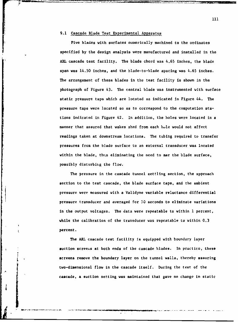
1ll
9.1 Cascade Blade Test Experimental Apparatus
Five blades with surfaces numerically machined to the ordinates
specified by the design analysis were manufactured and installed in the
ARL cascade test facility. The blade chord was 4.65 inches, the blade
span was 14.50 inches, and the blade-to-blade spacing was 4.65 inches.
The arrangement of these blades in the test facility is shown in the
photograph of Figure 43. The central blade was instrumented with surface
static pressure taps which are located as indicated in Figure 44. The
pressure taps were located so as to correspond to the computation sta-
tions indicated in Figure 42. In addition, the holes were located in a
manner that assured that wakes shed from each hule would not affect
readings taken at downstream locations. The tubing required to transfer
pressures from the blade surface to an external transducer was located
within the blade, thius eliminating the need to mar the blade surface,
possibly disturbirng the flow.
The pressure in the cascade tunnel settling section, the approach
section to the test cascade, the blade surface taps, and the ambient
pressure were measured with a Validyne variable reluctance differential
pressure transducer and averaged for 30 seconds to eliminate variations
in the output voltages. The data were repeatable to within 1 percent,
while the calibration of the transducer was repeatable to within 0.3
percent.
The ARL cascade test facility is equipped with boundary layer
suction screeics at both ends of the cascade blades. In practice, these
screens remove the boundary layer on the tunnel walls, thereby assuring
two-dimensional flow in the cascade itself. During the test of the
cascade, a suction setting was maintained that gave no change in static
J

112
to 000
04-4 W.
0 C34
to0
0w
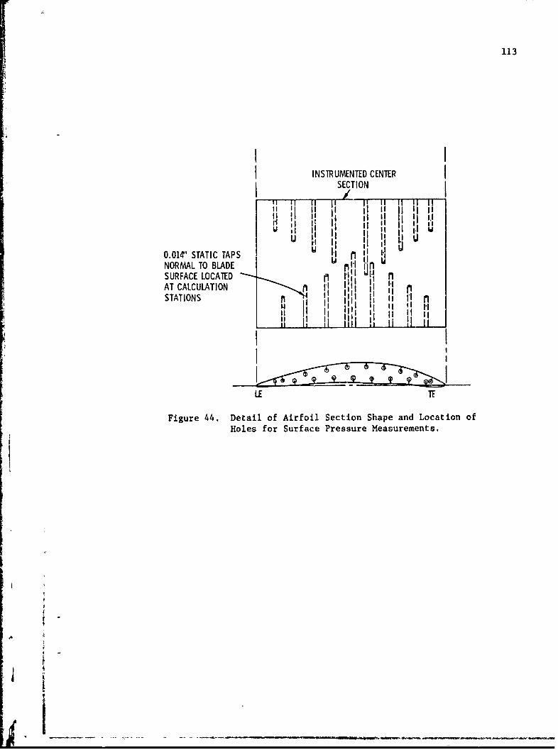
113
I INSTRUMENTED CENTERISECTbON
0.014"' STATIC TAPS 1.NORMAL TO BLADE i I.I I*InSURFACE LOCATED n ~ U~AT CALCULATION I Ii iSTATIONS ~ : It IPI n
LE IF
Figure 44. Detail of Airfoil Section Shape and Location ofHoles for Surface Pressure Measurements.

114
pressure along the approach duct to the cascz.de, indicating that two-
dimensional flow was maintaine~i.
A comparison of the flow field in the test cascade with the theo-
rctJ-.al flow field requires obýaining the velocities (V y) and (V )
parallel and perpendicular to ':he cascade axis, respectively, and the
local static pressure (P a) at various locatmons in the flow field. A
thre•-hole probe was fabricated and calibratcd for use in this experi-
ment. The mounting arrangemen.. of the probe In the ARL cascade facility
Is shown In Figure 43 and schenatically in F:gure 45. An expanded
schematic view of the probe ti; Is shown in g?,ure 46. The basis for
the design and calibration of .his probe is p.resented in Treaster and
Yocum [37]
Calibration of the three-?ýole probe was .ccomplished in the
following manner. The probe wýýs mounted in a retaining collar with the
probe tip located at the cente- of a 1.0 foot. diameter, low turbulence,
open jet. This arrangement is shown schemat'cally in Figure 47, The jet
velocity was maintained at 103 feet per secor'!, the maximum capability of
the facility. The probe Reyno'ds number, bared on the hole diameter, was
1080. The angle of the probe was systematicilly varied in small
increments from a flow angle rlative to the probe of -20 degrees to +20
degrees. At each setting, the pressures (P+, Pt, P) from the probe were
recorded. Additionally, the settling sectiort total pressure (1T) and the
Jet fare (atmospheric) pressure PS were recorded. These pressures are
repreusented schematically in I:igure 46. The Validyne variable reluctance
differe*ntial pressure transducý,r was used so that each recorded pressure
was the pressure difference ab!,ve the tntmosp|•eric referenced pressure.

115
THREE-HOLE TEST
SETTLING SECTION
-S AVERAGE PRESSURE INTUNNEL APPROACH
SECTION
j Figure 45. Three-Hole Probe and Cascade BladePTest Geometry.
I4 0
___ T E REEECELN
NOES P. ESRDNTNE

116
MEASURED 0.03Z' HYPODERMIC TUBINGPRESSURES
P+ __•• _•SOFT
V + O SOLDER
Pt ----- .PT PS 0 FILLET
P0
4TUBE FACES GROUND AS INDICATED
AND ETCHED WITH ACID TO REMOVEBURRS
Figure 46. Expanded View of Three-Hole Probe Tip.
SIt ..

117
OPEN-JET TUNNEL ~
CLAMP TOf /SET ANGLE
ADJUSTABLE-HEIGHT COLUMNTO KEEP PROBE TIP ONTUNNEL CENTERLINE
Figure 47. Three-Hole Probe Calibraticn in OpenJet Tunnel,
l- I

118
The pressures were averaged for 10 seconds to reduce variability, leading
to a repeatibility of 1 percent.
Three calibration coefficients are required to determine the two
velocity components and the static pressure at the probe tip. To deter-
mine the flow angle, the difference in pressure between the two side
pressure tubes P+ and P is used. The angularity correlation coefficient
(C P) is defined as
C (P+-P-) (9.1)Pa Pt - /2(P++P)
where the measured pressures are defined as in Figure 46. The result of
this calibration is plotted on Figure 48 as a function of flow angle (a)
relative to the probe axis.
Determination of the total pressure that exists at the probe loca-
tion is accomplished by a correlation of the measured total pressure Pt
and the actual total pressure PT' During calibration, PT is measured in
the calibration facility settling section. The total pressure correla-
tion coefficient (C~ ) is defined as
PT - PtC =- ,-. (9.2)Pt P - •/2(P++P)
t
These calibration data are plotted in Figure 49 as a function of the
flow angle (c).
The final calibration coefficient is used to determine the static
pressure at the probe tip. The correlation relates the average measured

119
2
0~
0.
S-3
-20 -1 £0 20
FLOW ANGLE, a
Figure 48. Three-Hole Probe CalibrationI,-I 1
' aA÷

120
'=- 0.3
0-0.2-
' 0.11
-0.1
-0. i-20 -10 0 10 20
FLOW ANGLE, a
Figure 49. Three-Hole Pribe Calibration(C p vs a).!t
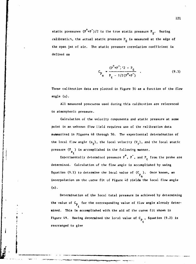
121
static pressures (P ++P-)/2 to the true static pressure PS. During
calibraticn, the actual static pressure PS is measured at the edge of
"the open jet of air. The static pressure correlation coefficient is
defined as
(P++P-,'2 - PS
C P S (9.3)s P - ./2(P +P-)t
These calibration data are plotted in Figure 50 as a function of the flow
angle (a).
All measured pressures used during this calibration are referenced
"I to atmospheric pressure.
Calculation of the velocity components and static pressure at some
Spoint in an unknown flow ileld requires use of the calibration data
summarized in Figures 48 through 50. The experimental determination of
the local flow angle (a ), the local velocity (V ), and the local static
pressure (P ) is accomplished in the following manner.
St+ -
Experimentally determined pressure P , P , and P from the probe aret
determined. Calculation of the flow angle is accomplished by using
Equation (9.1) to determine the local value of (C ). Once known, an
interpolation on the curve fit of Figure 48 yields the local flow angle
(a).
Determination of the local total pressure is achieved by determining
the value of C for the corresponding value of flow angle already deter-
mined. This is accomplished with the aid of the curve fit shown in
Figure 49. Having determined the local value of C~t, Equation (9.2) isPt
= rearranged to give
h

122
C%
a-
a-26
Q,'r
A 1.26
FO A" 1.23-
1.-2 -10 0 10 20
FLOW ANGLE, a
Figure 50. Three-Hole Probe Calibration(Cp vs a).
t8
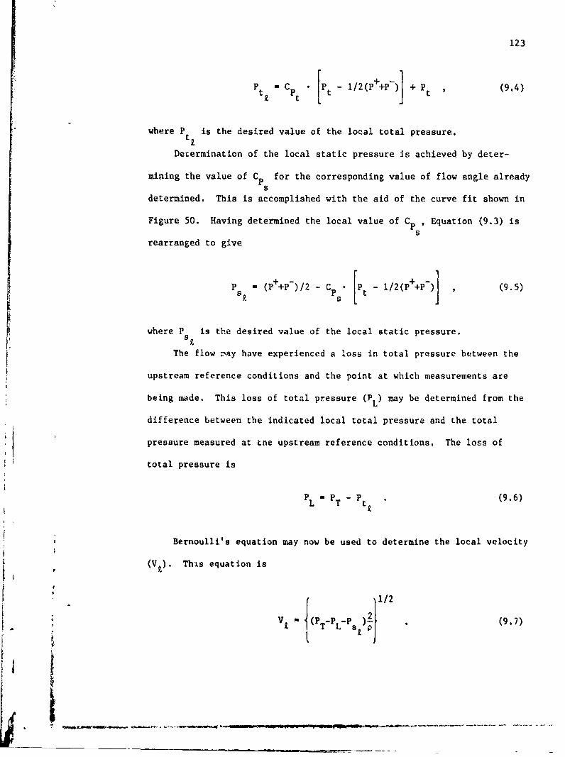
123
P C " P - 1/2(P++P-) + P (9.4)t z it t + t
where P is the desired value of the local total pressure.ti
Decermination of the local static pressure is achieved by deter-
mining the value of C for the corresponding value of flow angle alreadys
determined. This is accomplished with the aid of the curve fit shown in
Figure 50. Having determined the local value of Cp , Equation (9.3) isS
rearranged to give
P s (P++P-)/2 - Ft - l/2(P++P-) (9.5)s
where P is the desired value of the local static pressure.st
The flow "ay have experienced a loss in total pressure between the
upstream reference conditions and the point at which measurements are
being made. This loss of total pressure (PL) may be determined from the
difference between the indicated local total pressure and the total
pressure measured at tne upstream reference conditions. The loss of
total pressure is
PL = PT - P (9.6)
Bernoulli's equation may now be used to determine the local velocity
(V2 ). This equation is
i1/2
V (PT-PL-Ps) (9.7)VmfTL S . J
"t--- ~- -
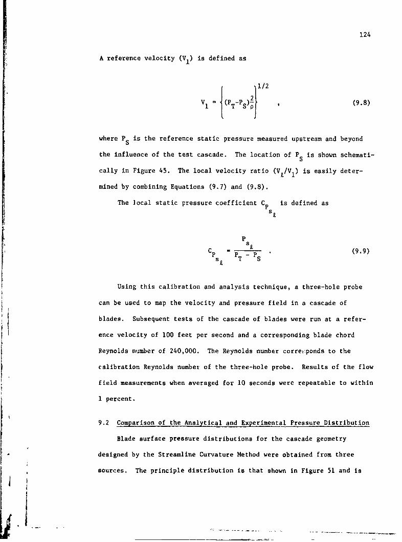
124
A reference velocity (V1 ) is defined as
VI (PT-Ps) /2 (9.8)
where PS is the reference static pressure measured upstream and beyond
the influence of the test cascade. The location of PS is shown schemati-
cally in Figure 45. The local velocity ratio (Vz/Vl) is easily deter-
mined by combining Equations (9.7) and (9.8).
The local static pressure coefficient C is defined ass i
PsCp P T PS (9.9)
Using this calibration and analysis technique, a three-hole probe
can be used to map the velocity and pressure field in a cascade of
blades. Subsequent tests of the cascade of blades were run at a refer-
ence velocity of 100 feet per second and a corresponding blade chord
Reynolds number of 240,000. The Reynolds number corret;ponds to the
calibration Reynolds number of the three-hole probe. Results of the flow
field measurements when averaged for 10 seconds were repeatable to within
1 percent.
9.2 Comparison of the Analytical and Experimental Pressure Distribution
Blade surface pressure distributions for the cascade geometry
designed by the Streamline Curvature Method were obtained from three
sources. The principle distribution is that shown in Figure 51 and is
1f
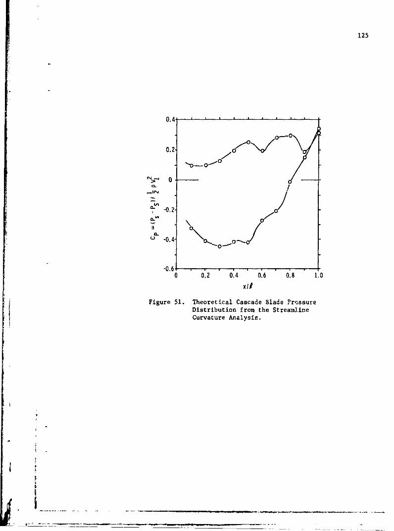
125
0.4
0
0.2 -O
">%• 0-0.
N1 4 0 0.o. . . .
X/-0. 0'/
-') -0.4 \ , 0.•0
0 0.2 0.4 0.6 0.8 1.0
x/ii
Figure 51. Theoretical Cascade Blade PrcssureDistribution from the StreamlineCurvature Analysis.
I

126
predicted by the design analysis. The design requires a fluid turning
angle of 18.43 degrees and a nondimensional flow diffusion, (V2 /VI), of
0.790, where VI is the velocity upstream of the cascade and V2 is the
velocity far downstream. The balance of blade forces to fluid momentum
changes requires that the average blade force per blade, in the direction
parallel to the cascade axis, be equal to the momentum change of the
fluid in the blade passage in the same direction. The equation
AP • C cos(O) = pSV xAV (9.10)x y
expresses this balance. (AP) is the average pressure difference across
the blade. Because the force parallel to the cascade axis is required,
the pressure acts on the projection of the blade chord (C) perpendicular
to the cascade axis (C.cos(8)). (8) is the angle of the vane relative to
the (x) direction and can be seen in Figure 42. The mass of fluid acted
on by the blade force per unit time is (pSV x), where (p) is the density,
(S) is the blade spacing, and (V x) is the velocity across the cascade.
The fluid momentum change is embodied in the term (AVy ), the change in
velocity parallel to the cascade axis, between the leading and trailing
edges. The quantities used in this discussion are depicted in Figure 42.
If the average blade pressure difference, (AP), is nondimension-
alized by the upstream dynamic pressure, as in the following relations,
V AV
Cp - AP/(l/2pV 2 2 (9.11)1 .CCos a VIV 1
a blade average loading or pressure coefficient (C-p) is formed. The test
case specified a design value of (Cp) of 0.6067. Integration of the
pressure distribution that is output of the design analysis yields a

127
value of Cp 0.440. Using Equation (9.10), the flow turning angle would
be 12.5 degrees using the reduced value of C-. This angle is 5.9 degreesP
less than the 18.43 degrees called for by the design.
As a check on the design geometry, the Douglass-Neumann potential
flow analysis method of Giesing [38] was performed. The pressure dis-
tribution of Figure 52 was generated. In this case, the value of Cp =
0.580, indicating a fluid turning angle of 17.4 degrees, was 1.0 degrees
less than called for by the design. Experience has shown that the
Douglass-Neumann analysis usually overestimates the turning that can be
performed by a cascade.
The Douglass-Neumann analysis indicated that the geometry was close
to conforming to the design but that the pressure distribution calculated
by the Streamline Curvature Method was in error.
A final comparison with the results from testing the design cascade
was made. The experimentally obtained pressure distribution is plotted
in Figure 53. The integrated value of C at the design conditions wasP
found to be 0.504, giving a flow turning angle of 14.7 degrees, 3.7
degrees less than design and 2.7 degrees less than predicted by the
Douglass-Neumann method.
Inspection of the pressure distributions shown in Figures 51, 52,
and 53 reveals that good agreement is obtained among the various compari-
sons for the pressure side of the blade. On the suction side, fair
agreement is maintained for the first 50 percent of the blade surface,
but at mid chord, the theoretical distribution from the Streamline
Curvature design analysis shows poor agreement with both comparison
cases. The conclusion here is that the lack of proper momentum force
4 balance noted previously is due to this discrepancy. Examination of the
W

128
0.6-
0.4
0.2CL
0~
-0.4
-0.6 -- "--0 0.2 0.4 0.6 0.8 1.0
x/#
Figure 52. Theoretical Cascade Blade PressureDistribution from the Douglass-Neumann Potential Flow Analysis.
I

129
0.4 0
"-0.2-
C.
-0.I4-
-0.6'
0 0.2 0.4 0.6 0.8 1. 0x/I
Figure 53. Experimental Cascade BladePressure Distribution,
-- ow
A -.t0

130
boundary layer calculations performed during the design indicated the
possibility of flow separation at 70 percent of the chord on the suction
surface, making the boundary layer and wake model inaccurate. Addition-
ally, experimental visual observations with tufts indicated that the
experimental blade was indeed separated in this area, possibly increasing
the observed underturning of the flow.
9.3 Comparison of the Analytical and Experimental Flow Fields
The velocity and pressure fields for the cascade design were
determined analytically upstream, within, and downstream of the blade
row. An experimental program using a three-hole probe determined the
corresponding flow field for the actual cascade. The results of the
experimental program are partially represented by the computer generated
plot of Figure 54. This figure shows the location of each data point
acquired, with the resulting velocity and direction shown.
Figure 54 shows the more important features of the flow field in the
cascade. First is an indication of a sepa.rated flow region on the
suction surface trailing edge. This region was also indicated by tufts
attached to the blade surface. The second most visible feature is an
indication of the extent and structure of the wake of low velocity fluid
shed from the blade trailing edges. Finally, the averaged fluid deflec-
tion angle at the downstream station is 13.5 degrees, agreeing fairly
well with the value determined by use of the pressure distribution.
More specific comparison of the analytical and experimental flow
fields are made in Figures 55 through 68. These figures are velocity
profile comparisons at each indicated reference station in Figure 42,

131
BLADE WAKE
BLADE GEOMETRYI\BLADE SUCTIONSURFACE
BLADE PRESSURE -SURFACE o
VELOCITY VECTORS
v. '00 MEASURED BY THE
0 /0 THREE-HOLE PROBE
SEPARA'(EDFFLOW REGION
Figure 54. Experimentally Determined Velocity Fieldin the Test Cascade.
V.•
I

132
5
THEORETICAL
EXPERIMENTAL
z 3--jUC-, 0zz
W- 2- 0
0
LUI
0zI-o
0-
-1-0.8 0.9 1.0 1.1 1.2
VmlV
Figure 55. Comparison of the Theoretical andE)ýperimental Velocity Profiles intie Test Cascade Reference Station20 Percent Blade Chord Upstream.
1i

133
SUCTIONSURFACE
4 o
U,
3- 0F_ 2
0
C-0)
zL.J
00
.LL
0 PRESSURE76 SURFACE
08 0.19 1.U 1.1 .2
LIv°M /VmVm
Figure 56. Comparison of the Theoretical andExperimental Velocity Profiles inthe Test Cascade Reference StationCoincident with Leading Edge.
ii
• ,a

134
5I- ---
SUCTIONSURFACE
-4
UCD
i-u 2. o0
00
0
00 PRESSUREa] SURFACE
0.8 0.9 1.0 1.1 1.2
Figure 57. Comparison of the Theoretical andExperimental Velocity Profiles inthe Test Cascade Reference SLztijnat 10 Percent of the Blade Chord.
_ _ _ _ _ _ - - - - - --t- - -

135
SUCTION4 SURFACE
UC
C-j
L" 2. 0
z0A~
0
00
I- 0
0 0 PRESSURESURFACE
-1.8 0.9 1.0 1.1 1.2
V IVmlI
Figure 58. Comparison of the Theoretical andExperimental Velocity Profiles inthe Test Cascade Reference Stationat 20 Percent of the Blade Chord.
I

136
5.
SUCTIONS4 SURFACE o
e-U 0
Lai_z 3- 0o
z
U- 2
oS000
0jz
0
00 0 PRESSURESURFACE
0.8 0.9 i.0 1.1 1.2
Figure 59. Comparison of the Theoretical andExperimental Velocity Profiles inthe Test Cascade Reference Stationat 30 Percent of the Blade Chord.

137
SUCTION
4- SURFACEw0
U 0_ 0
r-J
zu.J
0
0o 0 PRESSURESURFACE
0.8 0.9 1.0 1.1 1.2
VM IVIVmlV
Figure 60. Comparison of the Theoretical andExperimental Velocity Profiles inthe Test Cascade Reference Station
at ,0 Percent of the Blade Chord.
I,
~J77.~...

138
5-
4- SUCTIONSURFACE
U 0U4
-l
U 0A.
0
00
,,..1
Z
-0
0- o PRESSURESURFACE
-1-0.8 0.9 1.0 1.1 1.2
VM IVIi V~mlV
Figure 61. Comparison of the Theoretical andExperimental Velocity Profiles inthe Test Cascade Reference Stationat 50 Percent of the Blade Chord.
a,
-t- -.---.-- w ~ -~ -- ,-

139
5-
4- SUCTION 0SURFACE
U 0
3 0
-j
0z
Z 000EE
00
I- 0
S0 PRESSURE
SURFACE
0.8 0 .9 1 .0iol 1.2
Figure 62. Comparison of the Theoretical andExperimental Velocity Profiles inthe Test Cascade Reference Stationat 60 Percent of the Blade Chord.
J; -
i!

140
SUCTION_ SURFACE
CUu 0
3- 0-j
�) 0
WL&J
00
U.J
I-) 0
01 o PRESSURE
SURFACE
-110.8 0.9 1.0 1.1 1.2
VmlVV IVFigure 63. Comparison of the Theoretical and
Experimental Velocity Profiles inthe Test Cascade Reference Stationat 70 Percent of the Blade Chord.
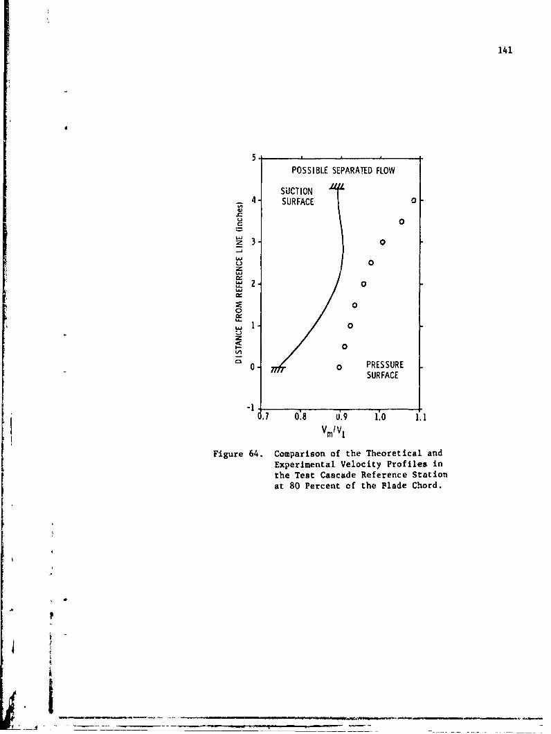
141
5-POSSIBLE SEPARATED FLOW
SUCTION4 SURFACE 0
3- 0
_00
L.=J
0 0z
2• 0
00
0z
0
0 0 PRESSURESURFACE
-1B7 0:8 u'.9 .1.1
VM/VIVmlV
Figure 64. Comparison of the Theoretical andExperimental Velocity Profiles inthe Test Cascade Reference Stationat 80 Percent of the Flade Chord.
It
F
L i _____

142
POSSIBLESEPARATED FLOW
SUCTION04 - SURFACE 0
- 0
z 3 0
LU
0
00Uj 0
00[ I-1 0
0 PRESSURE oSURFACE
0.1 0.8 om 9 .1.0 1.1
Figure 65. Comparison of the Theoretical andExperimental Velocity Profiles inthe Test Cascade Reference Stationat 90 Percent of the Blade Chord.
I
I,
I'

143
5 ,SUCTIONSURFACE SEPARATED FLOW
-4'C 0L-
C_ 0
z 3-o-JLAJ
L) 0z
2 0
0
0
I-. 0
SPRESSURE oSURFACE
POSSIBLE SEPARATED FLOW
0.7 0.8 0.9 1.0 1.1
v IV,
Figure 66. Comparison of the Theoretical andExperimental Velocity Profiles inthe Test Cascade Reference Station
Coincident with Trailing Edge.
I.
V.
1. t

144
5.PREDICIED WAKE
4 0-C 0
J--
0
LU
3. 0
00
U-
2- 0
00
Uj 0
z0
00So o.-..-__--o -°
0 00-1..6 0.7 0:8 0.9 0-- 0
Vm/V
Figure 67. Comparison of the Theoretical andExperimental Velocity Profiles inthe Test Cascade Reference Station20 Percent Blade Chord Downstream.

145I5-
00'N0
3- 0ýO
0Ui o
03 0
z
0-0
000
0. 6 .70l 0.10
F.s oz
0
-1 -, , '---0.6 0.7 O.g 0.9 1.0
VmlV
S~Figure 68. Comparison of the Theoretical and
Experimental Velocity Profiles inthe Test Cascade Reference Station
50 Percent Blade Chord Downstream.
_ _ _ _ _ _ _

146
Examination of the velocity profiles on each reference station
reveals the following. Agreement between experiment and analytical
results is good up to 40 percent of the blade chord. Figure 55 repre-
sents a station 20 percent of the chord upstreamn of the blade row. The
i signi'icant feature of this plot is that there are induced velocity
effects propagated upstream which are represented by the analysis method.
Also seen in this plot is an indication that the periodic nature of the
flow is not precisely maintained at this station, due to the required
cusping of the stagnation streamline at the blade leading edge. The
localized error, however, is only on the order of 3 percent.
Figures 56 through 59 show excellent agreement of the predicted and
experimental velocity profiles, both in magnitude and form.
Between 40 percent and 60 percent of the blade chord (Figures 60
through 67), some divergence in magnitude of the profile is seen. The
differences increase to the pofnt where, at 60 percent of the chord, the
measured velocity is uniformly 5 percent high. This is due to the blade
row underturning, because the blade row design is diffusing, rather than
accelerating, the flow.
From 70 percent to 100 percent of the chord, substantial (10 per-
cent) errors in the velocity profiles are seen. A definite indication
is present of the floo separation seen both on the pressure distribution
and by the tuft met'iod. Again, due to the blade row underdiffusing the
flow, the indicated measured velocities are uniformly high.
Downstream of the cascade, the measured data clearly indicate the
extent of the ,hed wake (Figures 67 and 68). Also seen is the failure
of the analytical method to accurately model the wake structure. In

147
general, the measured velocities are 13 percent too high, due again to
the blade row underturning.
6 An additional investigation was performed to help gain insight into
the physical phenomenon associated with the cascade underturning. A tuft
approximately 2 feet long was attached to the trailing edge pressure side
of the central blade in the cascade. A protractor was used to measure
the exit flow angle of the cascade relative to the inflow direction.
These measurements were accurate to 1/2 degree and result in the plot of
Figure 69. In the case of the as-designed data, there are three distinct
flow regimes. Below a Reynolds number of 210,000, severe underturning is
seen. This is probably due to a laminar separation at the minimum pres-
sure point on the blade suction surface. Above this condition, the
turning angle steadily increases to a steady value at a Reynolds number
of 300,000, indicating a partial Lurbulent separation that moves toward
the trailing edge as the velocity increases. As a test of the separation
theory, a cloth tape trip, one-eighth inch wide was attached to each
blade at 60 percent of the blade chord. Testing vBelded the second curve
on Figure 69. The turning angle with the tripped boundary layer is
nearly constant, indicating that a separated boundary layer is respon-
sible for the variation in turning angle with velocity or Reynolds
number. The test cascade was designed to operate at a Reynolds number
of 240,000, as indicated on Figure 69. The turning angle at this
velocity agrees with that determined by the pressure distribution
measurements and by the flow field surveys.
Pressure distributions were determirnd in each of the major flow
regimes noted on Figure 69. These pressure distributions are plotted on
Figure 70, and their corresponding velocities noted. The most
148
16-
z
A |A
&I OAS DESIGNED
""13 L I 7iRIP AT 60%,C SUCTION< LAMINARI
SEPARA- 0 FLOW-FIELD SURVEYS12 TION "
o12-
11 20250 360 350
BLADE REYNOLDS NUMBER x 1-
Figure 69. Cascade Turning Angle as a Function ofBlade Chord Reynolds Number.

149
REYNOLDS . .NUMBER
0.4 01I0,000
a 240,000
0.2
0
01
O,,'-%j -0.2'I
-0.4
-0.6
0.2 0.6 0.8 1.0
xlt•
Figure 70. Experimental Cascade Blade PressureDistribution as a Function of BladeChord Reynolds Number.
V
I
150
interesting feature of this plot involves the pressure distribution for
the lowest velocity case. Compared to the two higher velocity pressure
distributions, a severe difference in pressure on the suction side can
be seen. This indicates again the possibility of flow separation,
perhaps initiated at 40 percent of the blade chord. At the highest
velocity, the pressure distribution at the trailing edge is somewhat
fuller, accouating for the additional turning noted previously.
Because of the possibility of laminar separation affecting the
performance of the cascade, the turbulence level of the cascade test
facility was measured with a hot wire annemometer and found to be on the
order of 0.5 percent of the free stream velocity, which is quite low.
This could account for the unexpected laminar separation and for the
effect of the trip on the cascade performance. Additionally, the cor-
relations used in the development of the boundary layer model used on the
design process give no insight into the effect of the over-all turbulence
level on the shape or extent of the boundary layer.
9.4 Summary of the Analytical and Experimental Comparisons
Examination of the analytical and experimental data available pointA
to a major source of the problems encountered in this design. The
ability to accurately predict the boundary layer -haracteristics on the
suction side of the blades led to serious performance degradation. In
addition, the wake model, influenced by the boundary layer, was unac-
ceptable. A more accurate boundary layer model usable for boundary
layers in an increasing pressure zone must be developed and included in
the Streamline Curvature blade design method before a critical judgement
of Its usefulhess can be made.
151
Further examination of the output of the blade design analysis,
specifically Figure 42, shows that some rftnements to the computational
,chere are in order. To asqure that the far upstream and downstream
flow I.,i• uniform and parallel., the calculal Ions should be performed to
,;everal chord lengths in both directions. Figure 42 indicates some
:onwergence of the streamliies at the last calculation station, due to
the presence of the wake. "his region sh ild be extended to achieve
parallel flow. Increasing _-he number of calculation stations, stream-
lines, and cycles to conver ,ence should Wt.prove the over-all accuracy of
theL meLthod.
CHAPTER X
SUM14ARY, CONCLUSIONS, AND RECOMMENDATIONSFOR FURTHER RESEARCH
10.1 Summary and Conclusions
The design and analysis of a ,rbomachine requires a method for
predicting the three-dimensional flows which occur, along with methods
of designing blade rows which produce the desired performance. A large
class of turbomachines operate in flows which can be considered as being
incompressible. These include axial, mixed, and radial flow pumps and
turbines and low speed fans. The intent of this study is the development
of a rational engineering solution for the analysis and design of these
turbomachines.
The over-all performance of a turbomachine is related to the axi-
symmetric through-flow field within it. Various parameters affect the
through-flow, including the duct or casing geometry, the fluid velocity
and pressure at the inlet of the turbomachine, the geometric characteris-
tics of the blade rows which change the total energy of the fluid, and
the losses in energy due to viscous and turbulence effects. The accurate
predicting of this through-flow field must consider all of these boundary
I conditions and satisfy the laws of fluid motion. A computerized numeri-
I cal analysis has been developed to solve the equations of motion and
I } satisfy these boundary conditions.
the A Streamline Curvature Method is utilized as the basic solution for
the through-flow. Equations for a steady, inviscid, incompressible flow
tI
_It-

153
in an arbitrary shaped turbomachine are derived and a numerical method
developed for their solution.
The equations of motion are developed in a way that allows the
effects of blade spanwise and chordwise loading distributions to be
included in the solution. This is an improvement over some earlier
methods that treat a blade row as a thick actuator disk with uniform
chordwise loading.
The effects of the blade thickness distribution and blade surface
boundary layers may be incorporated into the solution. This point is
important when high solidity blade rows are used.
The effects of viscosity and turbulence on the through-flow are very
difficult to determine analytically; therefore, correlational data for
specific types of turbomachines are used to correct the through-flow
solution for these effects. The effects of viscosity and turbulence are
included as a distributed total pressure loss. Determination of the
specific distribution must rely on tests of turbomachines having a
similar geometric form.
Blade rows whose surfaces are not perpendicular to the axisymmetric
streamsurfaces in the turbownRchine produce a component of blade force
normal to the streamsurfaces. In some cases, this component can produce
a significant effect on the through-flow. The magnitude of this force
may be determined from the solution of the blade-to-blade flow fields on
the individual streamsurfaces and included in the through-flow solution
as a circumferentially-averaged pressure gradient nrrmal to the stream-
surfaces.
Several examples show the through-flow solution based on the
Streamline Curvature Method to be accurate in predicting the
.-6-.

154
axisymmetric properties of the flow in turbomachines. The design of
blade rows to provide a specified performance is difficult because of
the effects of viscosity and turbulence. t3 with the through-flow
analysis, it is necessary to include these effects in an empirical
fashion. The Mean Streamline Method of Wislicenus uses correlations
developed from experimental data to specify airfoil sections with a
specified chordwise loading distribution and includes the effects on
fluid turning due to viscosity and turbulence. The original correlation
as developed by Wislicenus is based on a small number of experimental
investigations A computerized method of analyzing the data generated
by the testing of airfoils in two-dimensional caszades is developed.
A large volume of data for airfoil sections tested in a cascade are
analyzed, the results are compared to the original data prepared by
Wislicenus, and a new correlation is developed which extends the range
of applicability of the Mean Streamline Method.
The improved Mean Streamline Method is adapted to the digital
computer and can be used rapidly and reliably by a designer. Due to the
complex nature of the flow between individual blades in a cascade, an
analytical approach to the solutior of the blade-to-blade flow field is
desirable. This solutiou allows the effect of each of the geometric and
flow parameters to be determined separately. Several methods for the
analysis of the blade-to-blade flow field for defined geometries exist.
However, an indirect or design solution which prescribes a blade shape
which will provide a specified performance has been elusive.
A Streamline Curvature Method is developed to solve the indirect or
design blade-to-blade flow problem. The solution relies on the numeri-
cal solution of the steady, inviscid, incompressible equations of fluid

155
motion, with the results corrected for the effects of viscosity and
turbulence. The solution starts with a blade shape defined by the Mean
Streamline Method and iteratively adjusts the camber line and thickness
distribution to satisfy the prescribed boundary conditions. These
boundary conditions include the specification of the chordwise loading
and thickness distributions and the periodicity of the flow field
upstream and downstream of the cascade. An empirical correction to the
flow field is made to account for the effects of the blade surface
boundary layers and the blade wake. The result 4f this analysis is a
cascade blade geometry and the associated flow field in the blade-to-
blade plane, which provides a specified performance.
An empirical cascade of blades was designed and tested in a cascade
wind tunnel to verify this analysis. The experimental results indicate
the potential of the design method to predict the flow field when the
effects of viscosity and turbulence are small. However, serious diffi-
culties were encountered in the boundary layer and wake regions of the
flow field and suggested that more sophisticated models of these regions
must be used.
The blade-to-blade flow solutions allow the computation of pressure
gradients normal to the streamsurfaces in a turbomachine. These terms
may be input to the through-flow solution to improve its accuracy in the
region of the blade row and, thus, produce a three-dimensional model of
tie flow field in the blade row.
An axial flow pump stage was designed by the Streamline Curvature
Method and the Mean Streamline Method and tested in a pump loop. Test
results indicate that the total pressure rise through the stage is 13
j percent higher than predicted. Analysis of the results reveals that the

156
experimental inflow velocity distribution is not the same as the design
inflow or that anticipated for the actual application of the pump.
Additionally, the estimated efficiency of the pump was probably too low
during the preliminary design phase, contributing to the increased value
of total pressure rise observed in the experimental results.
10.2 Recommendations for Further Research
The Streamline Curvature Method for predicting the axisymmetric
through-flow in turbomachines can be improved and extended by considering
the following areas of future research. The empirical correlations which
are employed to include real flow effects can be made more general for
axial flow units. This will require the testing and analysis of dif-
ferent configurations of axial flow pumps and turbines. Radial and mixed
flow turbomachines are more difficult to design and their internal flow
processes, especially boundary layer flows, are poorly understood. The
Streamline Curvature Method developed in this study can be used for the
prediction of the flow in a radial flow pump or turbine. Tests should be
designed to provide the analysis with the same type of correlation data
as used in the axial flow case.
The Mean Streamline Method of blade section design has been reliably
employed for axial flow turbomachinery and two-dimensional cascadeb. A
major improvement, including the capability to design blade sections in
conformal planes would allow the application of this design method to
mixed flow aad perhaps radial flow turbomachinery. Experimental verifi-
cation of the design method will be necessary to prove its usefulness
Sand accuracy.

157
The Streamline Curvature Method developed in this study to design
cascade airfoil sections will require a great deal of additional effort
before reliable designs can be produced. The numerical solution of the
equations can be improved by increasing the density of the calculation
stations and number of streamlines used in the solution. The empirical
data used to predict the boundary layer and wake effects will require a
test and analysis program, along with an advanced theoretical approach
to produce useful design correlations that properly account for Reynolds
number effects. A series of two-dimensional cascade lests with accurate
measurements of the boundary layer and wake profiles will help to produce
the required correlations.
The development of a three-dimensional design solution for turbo-
machinery is required if maximum possible performance is to be obtained.
An important part of this solution is the blade-to-blade flow solution.
The Streamline Curvature Method of blade section design produces this
flow field as a part of the design process. Improvements will have to
be made, however, before the solution is reliable. Again, experimental
comparisons of the flow fields in two-dimensional cascades will be
necessary to improve the solution. Of great importance here is the
experimental determination and comparison of the blade-to-blade flows in
a rotating blade row.
The effects of blade body forces on the through-flow solution
should be studied in greater depth. Occasionally, the blade geometry
leads to significant components of the blade force normal to the stream-
sLrfaces. This causes redistribution of the through-flow and, conse-
quently, changes the performance of the turbomachine. A large rotating
blade row, which exhibits a geometry leading to a streamsurface normal

158
force should be fully instrumented and its through-flow analyzed and
compared to a theoretical solution.
When the blade-to-blade and through-flow solutions have been
developed, a three-dimensional design solution can be developed by
analytically coupling the two-dimensional solutions. In this solution,
the blade row design is produced as a result of the specification of the
through-flow. All effects of blade row forces, loading distributions,
blade thickness, and the effects of viscosity and turbulence will be
included and solved simultaneously. The output of such a procedure is
the three-dimensional flow field in the blade-to-blade space and a blade
geometry required to produce the flow field. If five blade-to-blade and
meridional planes are specified as a minimum, the problem will require
at least twenty times the computer power and complexity currently re-
quired. However, as testing of turbomachinery becomes more expensive
and performance is pushed to higher levels, numerical design, modeling,
and testing will become more attractive and more important. Comparison
with experimental data will always be necessary to assure that the
physical processes involved are understood and that the empirical data
necessary to refine calculated flow models are accurate.
Improvement of the performance of turbomachinery operating in steady
incompressible flow will require the continued refinement and expansion
of numerical and mathematical flow modtls. The basic means of analysis
and design presented in this study can be used and improved and will lead
ultimately to the design of turbomachines that are more systematic and
reliable and with improved levels of performance.

159
REFERENCES
1. Wu, C. H., "A General Theory of Three Dimensional Flow in Subsonicand Supersonic Turbomachines of Axial, Radial, and Mixed FlowTypes," National Advisory Committee on Aeronautics, NACA TN 2604,1952.
2. Wislicenus, C. F., Fluid Mechanics of Turbomachinery, New York,N. Y., Dover Publications Inc., 1965.
3. NASA Staff, Aerodynamic Design of Axial Flow Compressors, NASASP-36, 1965.
4. Smith, L. H., Jr., "The Radial Equilibrium Equation of Turbo-machinery," Trans. ASME, J. Eng. Power, 88A, 1, 1966.
5. Marsh, H., "A Digital Computer Program for the Through Flow FluidMechanics in an Arbitrary Turbomachine Using a Matrix Method,"Aeronautical Research Council, ARC R&M 3509, 1966.
6. Katsanis, T., "Use of Arbitrary Quasi-Orthogonals for CalculatingFlow Distribution in the Meridional Plane of a Turbomachine," NASATN D-2546, December 1964.
7. Novak, R. A., "Streamline Curvature Computing Procedures fcr FluidFlow Problems," Trans. ASME, J. Eng. Power, Vol. 89, 1967.
8. Bosman, C,, and H. Marsh, "An Improved Method for Calculating theFlow in Turbomachines, Including a Consistent Loss Modefl," J. Mech.Eng. Sci., 1974.
9. Davis, W. R., and D. A. J. Miller, "A Comparison of the Matrix andStreamline Curvature Methods of Axial Flow Turbomachinery Analysis,from a User's Point of View," Trans. ASME, J. Eng. Power, January1975.
10. McBride, M. W., "A Streamline Curvature Method of AnalyzingAxisymmetric Axial, Mixed, and Radial Flow Turbomachinery," AppliedResearch Laboratory TM 77-219, The Pennsylvania State University,July 1977.
11. Billet, M. L., "An Approximate Method for the Solution of the DirectProblem of an Open Rotor," Applied Research Laboratory TM 78-161,The Pennsylvania State University, May 1978.
12. Brophy, M. C., Computer Assisted Design of Pump Impellers," AppliedResearch Laboratory TM 78-02, The Pennsylvania State University,January 1978.
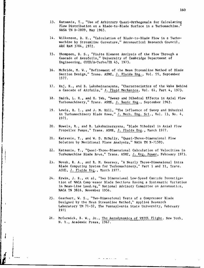
160
13. Katsanis, T., "Use of Arbitrary Quasi-Orthogonals for CalculatingFlow Distribution on a Blade-to-Blade Surface in a Turbomachine."NASA TN D-2809, May 1965.
14. Wilkenson, D. H., "Calculation of Blade-to-Blade Flow in a Turbo-machine by Streamline Curvature," Aeronautical Research Council,ARC R&M 3704, 1972.
15. Thompson, D. S., "Finite Element Analysis of the Flow Through aCascade of Aerofoils," University of Cambridge Department ofEngineering, CUED/A-Turbo/TR 45, 1973.
16. McBride, M. W., "Refinement of the Mean Streamline Method of Blade
Section Design," Trans. ASME, J. Fluids Eng., Vol. 99, September1977,
17. Raj, R., and B. Lakshminarayana, "Characteristics of the Wake Behinda Cascade of Airfoils," J. Fluid Mechanics, Vol. 61, Part 4, 1973.
18. Smith, L. H., and H. Yeh, "Sweep and Dihedral Effects in Axial FlowTurbomachinery," Trans. ASME, J. Basic Eng., September 1963.
19. Lewis, R. I., and J. M. Hill, "The Influence of Sweep and Dihedralin Turbomachinery Blade Rows," J. Mech. Eng. Sci., Vol. 13, No. 4,1971.
20. Howels, R., and B. Lakshminarayana, "Blade Dihedral in Axial FlowPropeller Pumps," Trans. ASME, J. Fluids Eng., March 1977.
21. Katsanis, T., and W. D. McNally, "Quasi-Three-Dimensional FlowSolution by Meridional Plane Analysis," NASA TM X-71593.
22. Katsanis, T., "Quasi-Three-Dimensional Calculation of Velocities inTurbomachine Blade Rows," Trans. ASME, J. Eng, Power, February 1973.
23. Novak, R. A., and R. M. Hearsey, "A Nearly Three-Dimensional IntraBlade Computing System for Turbomachinery," Part I and TI, Trans.ASIT4, J. Fluids Eng., March 1977.
24. Erwin, J. R., et al, "Two Dimensional Low-Speed Cas:ade Investiga-tion of NACA Comp-essor Blade Sections Having a Systematic Variationin Mean-Line Loading," National Advisory Committee on Aeronautics,NACA TN 3816, November 1956.
25. Gearhart, W. S., "Two-Dimensional Tests of a Compressor BladeDesigned by the Mean Streamline Method," Applied ResearchLaboratory TM 71-32, The Pennsylvania State University, February1971
26. McCormick, B. W., Jr., The Aerodynamics of VSTOL Flight, New York,N. Y., Academic Press, 1967.
h
L

161
27. Schlicting, H., "Application of Boundary Theory in Turbovachinery,"Trans. ASME, J. Basic Eng., Series D, Vol. 31, pp. 543-551, 1959.
28. McBride, M. W., "Computerization of the Mean Streamline Blade DesignMethod," Applied Research Laboratory TM 73-22, The PennsylvaniaState University, February 1973.
29. Wislicenus, G. F., and L. R. Smith, "Hydraulic Jet Propulsion andIncipient Cavitation," Internal Flow Research Report 1-6, Part A,The Johns Hopkins University, Mechanical Engineering Department,March 21, 1952.
30. Shephard, D. G., Principles of Turbomachiriery, 6th printing, TheMacmillan Company, 1965.
31. Vennard, J. K., Elementary Fluid Mechanics, 4th ed., New York,N. Y., John Wiley and Sons, 1961.
32. Davis, R. F., "Marine Propulsor Blade Section Definition," OrdnanceResearch Laboratory TM 513-3531-04, The Pennsylvania StateUniversity, February 1969.
33. Abbott, I. H., and A. E. Von Doenhoff, Theory of Wing Sections,New York, N. Y., Dover Publications Inc.
34. Truckenbrodt, E., "A Method of Quadrature for Calculation of theLaminar and Turbulent Boundary Layer in Case of Plane and Rotation-ally Symmetric Flow," National Advisory Committee on Aeronautics,NACA TN 1397, May 1955.
35. Schlicting, H., Boundary Layer Theory, New York, N. Y., McGraw-HillBook Co., Inc., 1960.
36. Horlock, J. H., Axial Flow Compressors, Butterworths, London, 1958.
37. Treaster, A. L., and A. M. Yocum, "The Calibration and Applicationof Five-Hole Probes," Proceedings of the 24th InternationalInstrumentation Symposium, Albuquerque, N. M., 1978, InstrumentSoc. of America.
38. Geising, J. P., "Extension of the Douglass-Neumann Computer Programof Problems of Lifting Finite Cascades," U. S. Dept. of Commerce,Report No. AD 605207.
JI
S
4j
DISTRIBUTION LIST FOR UNCLASSIFIED TM 79-33 by Mark W. McBride, datedFebruary 13, 1979
Commander Naval Ocean Systems CenterNaval Sea Systems Command Attn: D. NelsonDepartment of the Navy Code 6343Washington, DC 20362 (Copy No. 22)Attn: Library
Code NSEA-O9G32 Commander(Copy Nos. 1 and 2) Naval Ship Engineering Center
Department of the NavyF ' val Sea Systems Command Washington, DC 20361Attn: E. G. Li.zka Attn: D. V. Burke
Code SEA 63R-1 Code NSEC 6140B.1(Copy No. 3) (Copy No. 23)
Naval Sea Systems Command CommanderAttn: T. E. Peirce Naval Surface Weapon Center
Code SEA 63R-31 Silver Spring, MD 20910(Copy No. 4) Attn, Library
(Copy No. 24)Naval Sea Systems CommandAttn: A. R. Paladino Commander
Code SEA 05H David W. Taylor Naval Ship R&D Center(Copy No. 5) Department of the 4avy
Bethesda, MD 20084Defense Documentation Center Attn: R. J. Boswell5010 Duke Street Code 1544Cameron Station (Copy No. 25)Alexandria, VA 22314(Copy Nos. 6 - 17) David W. Taylor Naval Ship R&D Center
Attn: R. A. CummingCot.manding Officer Code 1544Naval Underwater Systems Cepter (Copy No. 26)Newport, RI 02840Attn: J. F. Brady David W. Taylor Naval Ship R&D CenterI (Copy No, 18) Attn: W. K. Blake
! Code 1942
Naval Underwater Systems Center (Copy No. 27)Attn: Library
Code 54 David W. Taylor Naval Ship R&D Center(Copy No. 19) Attn: W. B. Morgan
Code 154
Commanding Officer (Copy No. 28)
Naval Ocean System:n CenterDepartment of the Navy David W. Taylor Naval Ship R&D CenterSan Diego, CA 92152 AtLn: M. SevikAttn: J. W. Hoyt Code 19
Code 2501 (Copy No. 29)• upy No. 20)
Of f icr- in-ChargeNavai, Occan Systems Center David W. Taylor Naval Ship R&D CenterAttn: A.... Fabula Department of the Navy
6od)e S311 Annapolis Laboratory(Copy No. 21) A.-napoiis, MD 21402
Attn: J. G. StrickerCode 2721
(Copy No. 30)
4aa a a a a4a a a

DISTRIBUTION LIST FOR UNCLASSIFIED TM 79-33 by Mark W. McBriae, Qateurebruary 13, 1979
David W. Taylor Naval Ship R&D Center NASA Ames Research CenterAnnapolis Laboratory Moffett Field, CA 94985Attn: M. C. Brophy Attn: Library
Code 2721 (Copy No. 40)(Copy No. 31)
NASA Ames Research CenterNaval Postgraduate School Attn: F. BodapatiMonterey, CA 93940 MA 227-9Attn: Library (Copy No. 41)
Code 0212(Copy No. 32) NASA Liagley Research Center
Hampton, VA 23365Philadelphia Naval Shipyard Attn: LibraryU. S. Naval Base (Copy No. 42)Philadelphia, PA 19112Attn: F. Halpin Air Force Aero Propulsion Laboratory
Code 260.6 Wright-Patterson Air Force Base(Copy No. 33) Ohio 45433
Attn: LibraryBureau of Reclamation (Copy No. 43)U. S. Department of the InteriorEngineering and Research Center Air Force Office of Scientific ResearchRoom 28, Bldg. 56 1400 Wilson BoulevardP. 0. Box 25007 Arlington, VA 22209Denver Federal Center Attn: Dr. J. F. MasiDenver, CO 80225 (Copy No. 44)Attn: Dr. Henry T. 'alvey(Copy No. 34) National Technical Information Service
Department of CommerceNASA Lewis Research Center 5285 Po-t Royal Road21000 Brookp,.k Road Springfield, VA 22151Cleveland, OH 44135 Attn: Chief '"iut SectionAttn: N. C. Sanger (Copy No.
MS 5-9(Copy No. 35) Office of Naval Research
Department of the NavyNASA Lewis Research Center Arlington, VA 22217Attn: M. J. Hartmann Attn: J. Patton
MS 5-9 (Copy No. 46)(Copy No. 36)
Detroit Diesel Allison DivisionNASA %ewis Research Center P. 0. Box 894Attn: D. M. Sandercock Indianapolis, IN 46206
MS 5-9 Attn: Library(Copy No. 37) (Copy No. 47)
NASA Lewis Research Center Garrett CorporationAttn: W. M. McNally AiResearch Manufacturing Company
MS 5-9 Sky Harbor Airport(Copy No. 38) 402 South 36th Street
Phoenix, AZ 85034NASA Lewis Research Center (Copy No. 48)Attn: Library(Copy No. 39) General Electric Company
Cincinnati, Ohio 45215Attn: Libr3ry(Copy No. 49)

DISTRIBUTION LIST FOR UNCLASSIFIED TM 79-33 by Mark W. McBride, datedFebruary 13, 1979
General Electric Company Calspan CorporationCorporate Research and Development 4455 Genessce StreetP. 0. Box 8 Buffalo, NY 14221Schenectady, NY 12301 Attn: Head LibrarianAttn: Library (Copy No. 58)(Copy No. 50)
MS-16 United TechnologiesLTV Vought Aeronautics Company Research CenterP. 0. Box 5907 Silver LaneDallas, TX 75222 E. Hartford, CT 06118Attn: Library Attn: E. M. Greitzer(Copy No. 51) (Copy No. 59)
Lockheed Propulsion Company Creare, Inc.Scientific and Technical Library Box 71P. 0. Box 111 Hanover, NH 03755Redlands, CA 92373 httn: W. SwiftAttn: Library (Copy No. 60)(Copy No. 52)
Rocketdyne DivisionMcDonald Aircraft Company North American AviationP. 0. Box 516 6633 Canoga AvenueSt. Louis, MO 63166 Canoga Park, CA 91303Attn: Res. & Eng. Library Attn: E. Jackson
Dept. 218 - Bldg. 101 Hydrodynamics Group(Copy No. 53) (Copy No. 61)
Pratt and Whitney Aircraft Division Aerojet GeneralFlorida Res. & Dev. Ctr. Post Office Box 15847P. 0. Box 2691 Sacramento, CA 15813West Palm Beach, FL 33402 Attn: Library(Copy No. 54) (Copy No. 62)
Pratt and Whitney Aircraft Division Hydronauti-s, Inc.United Aircraft Company Findell School RoLd400 S. Main Street Laurel, MD 20810East Hartford, CT 06108 Attn: J. BohnAttn: Library (Copy No. 63)(Copy No. 55)
California Institute of TechnologyAllis-Chalmers Corporation Jet Propulsion LaboratoryHydro-Turbine Division 4800 Oak Grove DriveBox 712 Pasadena, CA 91109York, PA 17405 At'n:. libraryALtn: R. K. Fisher (Copy No. 64)(Copy No. 56)
California Institute of TechnologyAllis-Chalmers Corp. Divis'3n of Enineering forAttn: W. Whippen Applied Sciences(Copy No. 57) Pasadena, CA 91109
Attn: Dr. Allan J. Acosta(Copy No. 65,

DISTRIBUTIC" LIST FOR UNCLASSIFIED TM 79-33 by Mark W. McBride, datedFebruary 13, 1979
Dr. George F. Wislicenus Professor J. H. Horlock351 Golf Court (Oakmont) Vice-ChancellorSanta Rosa, CA 95405 University of Salford(Copy No. 66) Salford, M5, 40T
EnglandMassachusetts Institute of Technology (Copy No. 75)77 Massachusetts AvenueCambridge, MA 02139 Dr. John FoxwellAttn: Technical Reports Admiralty Research Laboratory
MIT Libraries Teddington, MiddlesexRoom 14 E-210 England
(Copy No. 67) (Copy No. 76)
Massachusetts Institute of Technology Whittle Turbomachinery LaboratoryAttn: Eng. Tech. Reports Madingley Road
Room 10-408 Cambridge(Copy No. 68) England
Attn: LibraryVirginia Polytechnic Inst. & State Univ. (Copy No. 77)Blacksburg, VA 24061Attn: Library Whittle Turbomachinery Laboratory(Copy No. 69) Attn: Sir William Hawthorne
(Copy No. 78)Iowa State UniversityMechanical Engineering Department Whittle Turbomachinery LaboratoryAmes, IA 50010 Attn: Dr. D. S. WhiteheadAttn: Dr. G. K. Serovy (Copy No. 79)(Copy No. 70)
Dr. D. S. ThompsonPurdue University Turbine Research DepartmentThermal "cience & Prop. Center Rolls Royce Ltd.West Lafayette, IN 47907 P. 0. Box 31Attn: Dr. S. N. B. Murthy Derby(Copy No. 71) England
(Copy No. 80)University of PennsylvaniaTowne School of Civil & Mech. Eng. Professor R. E. PeacockRoom 113 Towne, 220 S. 33rd St. School of Mechanical EngineeringPhiladelphia, PA 19104 Cranfield Institute of TechnologyAttn; Dr. Hsuan Ych, Director Cranfield, Bedford MK430AL(Copy No. 72) England
(Copy No. 81)Stevens Institute of Technology711 Hudson Street Dr. Allen MooreCastle Point Station Admiralty Marine Technology Establish'Hoboken, NJ 07030 Teddington, MiddlesexAttn: S. Tsakonas EnglandkCopy No. 73) (Copy No. 82)
Stevens Institute of Technology J. LewisAttn: Dr. Bruce D. Cox University of Newcastle(Copy No. 74) Newcastle
England(Copy No. 83)
DISTRIBUTION LIST FOR UNCLASSIFIED TM 79-33 by Mark W.. McBride, datedrebruary 13, 1979
Dr. Peter van Oossanen The Pennsylvania State UniversityHaagsteeg 2 Applied Research LaboratoryPostbox 28 Post Office Box 306700 AA Wageningen State CoLlege, PA 16801The Netherlands Attn: W. S. Gearha,:(Copy No. 84) (Copy No. 90)
Von-Karman Institute for Fluid Dynamics Applied Research LaboratoryTurbomachinery Laboratory Attn: B. LakshminarayanaRhode-Saint-Genese (Copy No. 91)BelgiumAttn: Library Applied Research Laboratory(Copy No. 85) Attn: M. W. McBride
(Copy No. 92)Professor J. P. GostelowSchool of Mechanical Engineering Applied Research LaboratoryNSW Institute of Technology Attn: J. R. RossBroadway (Copy No. 93)SidneyAustrailia AppLied Research Laboratory(Copy No. 86) AttM. A. L. Treaster
(Cop) No. 94)Dr. rer. nat. Horst MerbtForschungsbeauftragter fiir Hydroakustik Applied Research Laboratory8012 Ottobrunn B Munchen Attn: Garfield Thomas Water TunnelWaldparkstr. 41 FilesMunich (Copy No. 95)Germany(Copy No. 87)
Carl-Anders JohnssonStatens SkeppsprovningsanstaltBox 24001S-400 22 GoetborgSweden(Copy No. 88)
Dr. V. H. ArakeriDepartment of Mechanical EngineeringIndian Institute of ScienceBangalore 560 012India(Copy No. 89)