THE DERIVE - NEWSLETTER #22 - Austromath · In the last time I received many interesting contributions to be published in the next DNLs. They all ... Parts of it will be the introduction

THE DERIVE - NEWSLETTER #22

ISSN 1990-7079 T H E B U L L E T I N O F T H E

U S E R G R O U P C o n t e n t s:

1 Letter of the Editor 2 Editorial - Preview 3 DERIVE User Forum Edward Sawada 8 IMP Spider and Misguided Missiles Thomas Weth 13 A Lexicon of Curves (8) – A Didactical Appendix Hartmut Kümmel / Jan Vermeylen 22 JULIA Sets with DERIVE Josef Böhm 25 Functions of Random Variables Carl Leinbach & Marvin Brubaker 29 Carl and Marvin´s Laboratory (2) Bernhard Wadsack 31 DREIECK.MTH – TRIANGLE.MTH 38 Johann´s Titbits – Some additional notes (The 17- Edge, Partitioners) 44 AC DC One Sergey V. Biryukov 46 Clear Function Parameters Representation Bert Waits, Bernhard Kutzler & Frank Demana 48 The TI-92 Corner (Chaos Game, Financial Maths a.o.)

revised Version 2010 June 1996

D-N-L#22

I N F O R M A T I O N - B o o k S h e l f

D-N-L#22

[1] Learning Modelling with DERIVE, Townend, Poutney

Prentice Hall, 244 pages, ISBN 0-13-190521-X

[2] ACTAS de las Jornadas sobre la enseñanza de matemáticas con Derive You can find some information in the User Forum, page 5.

[3] Der TI-92 im Unterricht, Klaus Aspetsberger u. Franz Schlöglhofer

[4] Mathematik erleben mit dem TI-92, Günter Schmidt

Both publications are available from Texas Instruments Deutschland, 85356 Freising (Tel:08161 804984)

Exchange for DERIVE Teaching materials in the DNL

The wheel has not to be invented twice.

Börse für DERIVE Unterrichts- materialien im DNL

Das Rad muss nicht zweimal erfunden werden.

I can offer: Binomial Theorem, GCD & LCM, System of coordinates, Modeling Word problems with DERIVE (all in English and German), SET.EXE, MENGE.EXE. Functions -Domain and Range from Tom Drummond, Glasgow. I have produced a paper "Einführung in die Matrizenrechnung mit DERIVE" -in German. If you are interested I would send you the paper on a diskette in MS-Word6-format.

In the last time I received many interesting contributions to be published in the next DNLs. They all were accompanied by friendly letters. I´ll reprint some sentences to give an idea about their contents:

David Halprin, North Balwyn, Australia: … I have opened a mathematical 'can of worms', too much for one person to develop to its full potential, so I invite fellow members of DUG or readers of the Newsletter to write to me (about the "Cesaro Glove-Osculant"). Maria Koth, Vienna, Austria: … Motiviert durch unser Gespräch auf der Lehrerfortbildungstagung habe ich jetzt meinen Artikel „Computergrafik mit DERIVE“ ("Computer Graphics with DERIVE") überarbeitet und möchte Ihnen die verbesserte Version zusenden … (about generators of fractals, Sierpinski triangles a.o.) Prof. M.J.Fernández Guitiérez, Oviedo, Spain: I now enclose copies of our manuscript "Solving third-order linear differential equations with constant coefficients", that I believe fits the requirements for papers in the DERIVE NEWSLETTER. So I would like you to consider it for publication … G P Speck, Wanganui, New Zealand: The DNL readers may find the catalogue of function tables presented with attendant MTH files a significant time saver as I have on several occasions. Peter Mitic, Medstead, England: I enclose three articles which you might look at. They are an extension of the talk I gave at the Plymouth conference in 1994, "Exploiting new Features in DERIVE 3", "The Normal Distribu-tion: two Proofs and a Simulation", "Probability Distributions: Proof and Computations" … Many thanks for your long and contentful letter. Parts of it will be the introduction to your contribution. I would like to receive your 'short notes' on the use of probability generating functions. I think that probability theory is a very important part of mathematics and we could enforce it in the DNL. So I published one teaching unit in this DNL which I wrote some time ago for use in my classes. Once more many thanks and much luck in your new career. Josef. Prof. Neil Stahl, Menasha, Wisconsin, USA: … For years I felt computer graphics would be of benefit in dem-onstrating important concepts in calculus, such as tangent lines and tangent planes as well as direction fields. I am pleased at the opportunity you are offering me to distribute this work more widely. Nurit Zehavi, Rehovot, Israel: I hereby submit a "DERIVE tip" to the DUG newsletter. I hope that you and other users will find it helpful. Many thanks to all of you. I think we all can be proud of the intemationality of our group and of its en-thusiasm, of course. We cooperate from country to country and from contintent to continent. Let´s pro-ceed on our way!

D-N-L#22

L E T T E R O F T H E E D I T O R

p 1

Liebe DUG Mitglieder, Ich habe versucht, in diesem DNL einige alte „Schulden“ zu begleichen, d.h. Beiträge aufzuneh-men, die schon lange auf meinem „Stack“ liegen. Anstelle der "TITBITS" finden Sie dieses Mal einige Anmerkungen und Ergänzungen zu den letzten Tit-bits. Ich finde den e-mail-Austausch besonders in-teressant, weil uns Albert Rich und Johann Wie-senbauer damit einigen Einblick in das Innenleben von DERIVE ermöglichen. Ich danke Alfonso J. Poblacion für die Anregung zum AC DC-Teil und auch dafür, dass er gleich den ersten Beitrag dafür geleistet hat. Ich möchte Sie gerne einladen, sich fallweise an der Gestaltung dieser - vielleicht ständigen - Kolumne des DNL zu beteiligen. Für die TI-92 Benutzer und solche, die es werden wollen, ist sicher interessant, dass ein von TI unterstütztes Fortbildungsprogramm T3 (Teachers Teaching with Technology), das in den USA unter der Leitung von Bert Waits und Frank Demana schon etabliert ist ,auch in Europa als T3-Europa eingeführt werden soll. Ich habe die Ge-legenheit, im Juni in Columbus, OHIO, an einer T3-Sommerschule teilzunehmen und kann im näch-sten DNL darüber berichten. Nun zwei Hinweise: Ihre DUG Mitgliedsnummer finden Sie auf dem Adressenaufkleber, und mit glei-cher Post sende ich die MTH-files zu diesem DNL nach Hawaii. Albert Rich hat zugesagt, diese nach Mög1ichkeit in seine web-Seite aufzunehmen. Viel Glück beim „Downloaden“! (http /www.derive. com). Wir freuen uns schon auf Bonn. Sie können als Vor-geschmack drei mit DERIVE berechnete Raumfigu-ren sehen. die ich mit einem Hilfsprogramm ins ACROSPIN-Format konvertiert habe. Damit kön-nen diese Figuren nun auch animiert werden. Mit den besten Grüßen, Ihr Josef Böhm

Dear DUG Members, I have tried to settle some old debts in this DNL, i. e. to publish contributions which have been waiting on my "stack" since long. Instead of the TITBITS you will find some completions to earlier articles. I find the e-mail exchange especially interesting because AIbert Rich and Johann Wiesenbauer give some insight into inside DERIVE. My special thanks go to to Alfonso J. Pobla-

cion not only for his idea to create AC DC but also for submitting the initial paper. I would like to encourage you to contribute to this - maybe permanent - new column. Certainly it is interesting for being and ongoing TI-92-Users, that T3 (Teachers Teaching with Technology) - a profess-ional development program, spons-ored by TI, which was founded

by Bert Waits and Frank Demana - will be es-tablished as T3-Europe in Europe. Fortunately I have the opportunity to attend the next T3 summer school at Columbus, OHIO in this June. I will give a report about this event in the next DNL. Two notes: You can find your DUG member-ship number on your address label, and I am mailing all the MTH-files belonging to this DNL issue to Hawaii. AIbert Rich has promised to put them on SWHH's website. Much luck with downloading. (http://www.derive.com) We are looking forward to the Bonn Confer-ence. As a foretaste you can see three DE-RIVE calculated 3D-objects which I converted into the ACROSPIN format using a self made program. It enables animating those figures using different colours and layers. With my best regards Josef

Conic sections Elliptic torus with a torus knot line and its tube

p 2

E D I T O R I A L

D-N-L#22

The DERIVE-NEWSLETTER is the Bulle-tin of the DERIVE User Group. It is pub-lished at least four times a year with a con-tents of 30 pages minimum. The goals of the DNL are to enable the exchange of ex-periences made with DERIVE as well as to create a group to discuss the possibilities of new methodical and didactical manners in teaching mathematics. We include a section dealing with the use of the TI-92.

Editor: Mag. Josef Böhm A-3042 Würmla D´Lust 1 Austria Phone: 43-(0)660 40 70 480 email: [email protected]

Contributions: Please send all contributions to the Editor. Non-English speakers are encouraged to write their contributions in English to rein-force the international touch of the DNL. It must be said, though, that non-English ar-ticles are very welcome nonetheless. Your contributions will be edited but not as-sessed. By submitting articles the author gives his consent for reprinting it in the DNL. The more contributions you will send, the more lively and richer in contents the DERIVE Newsletter will be.

Preview: (Contributions for the next issues): Graphic Integration, Linear Programming, Böhm, A LOGO in DERIVE, Lechner, A 3D Geometry, Reichel, A Parallel- and Central Projection, Böhm, A Algebra at A-Level, Goldstein, UK Tilgung fremderregter Schwingungen, Klingen, GER Utility for Complex Dynamic Systems, Lechner, A Some notes on DERIVE 2.6 functions and limits, Speck, NZL Linear Mappings and Computer Graphics, Kümmel, GER Solving Word Problems with DERIVE, Böhm, A DERIVE and ACROSPIN, Schorn & Böhm, A/GER Visualizing a Special Line in the 3D-Space, Zehavi, ISR Line Searching with DERIVE, Collie, UK The TI-92 Section, Bert Waits, Bernhard Kutzler, Frank Demana and

Setif, FRA; Vermeylen, BEL; Leinbach, USA, Aue, GER; Halprin, AUS; Weth, GER; Wiesenbauer, A; Keunecke, GER; Weller, GER; …

Impressum: Medieninhaber: DERIVE User Group, A-3042 Würmla, D´Lust 1, AUSTRIA Richtung: Fachzeitschrift Herausgeber: Mag. Josef Böhm Herstellung: Selbstverlag

D-N-L#22

D E R I V E - U S E R - F O R U M

p 3

Pierre A. Arnoldi, Vermont, Switzerland Derive for Windows will no doubt be of great interest to me. I am running an IBM compatible machine with EGA/VGA screen. My printer is a CANON BJC-70 (black and white and four colors printing head). I was not yet able to connect some fake-printer to the machine for my graphs to be printed in colors. Can you tell me which printer I should choose among all printers registered in Windows, which works the same way my Canon works (ink bubble system)? How am I supposed to select the DERIVE printing options then? … You should note that I am not a mathematician at all. I happened to study some algebra when I was young as well as geometry and other related branches of such sciences. I was more fascinated than really interested and I am not going to be another Einstein … DNL: I asked Micheal Petz from SWHH about your problem. Michael has a Canon BJ for his own (only black & white) and he is running his machine in Epson mode. He does not face any problem. I have tried with an HP-Deskjet Colour printer and had no problems, too. You can find the appropriate DeskJet C setting in the Transfer Print Options. Much luck for producing nice colour prints with DERIVE. John Berry, Plymouth, UK Dear Josef, HELP!! You are the DERIVE wizz, can you solve my problem below? This set of steps produces a part of the bifurcation diagram for the quadratic map x2 – c. I want to automate it for lots of values of c, plotting the answers. Any idea how I can do it please?

DNL: I hope that the “wizz” can help. If not then please don´t blame my wizzardry. Proceed with:

p 4


D-N-L#22

Helmut Wunderling, Berlin, Germany Ich habe Problem mit DERIVE 3 bei der Polynomdivision (komplex), obwohl ich mit Herrn Kutzler in Re-gensburg darüber gesprochen habe. Beispiel: p(z) := z4 + 5z3 – 3z2 + 15z – 7 – 2i; p(z) = 0 Eine Näherungslösung ist z1 = 0.4783 + 0.125866 i (über Newtonverfahren).

Die Division 1

( )p zz z−

geht „näherungsweise“ auf, was DERIVE nicht kennt (im Gegensatz zu Mathematica). Es

ist unschön, aus dem Wust der DERIVE-Terme diese Näherung zu bekommen, um weitere Nullstellen zu bestimmen. Gibt es Tricks?

Ich habe natürlich einen graphischen Ausweg, der den Hauptsatz der Algebra einsichtig macht. Besteht ein In-teresse daran?

Helmut Wuderling addresses problems dividing a complex polynomial p(z) by the linear factor (z – z1) with z1 being an approximate root of the equation p(z) = 0. Mathematica is able to perform this “ap-proximative” division which makes possible to find more zeros.

DNL: I have some ideas to solve your problem: Try Müller´s Method (DNL#20). Load MULLER.MTH from DNL#20 and then proceed:

This method does without explicitly dividing the polynomials.

D-N-L#22


p 5

DERIVE 6 should do better, because there is a QUOTIENT-function which could do the job, but:

In 1996 I tried to implement Horner´s algorithm to reduce the order of the polynomial. The POLY_DEGREE-function did support complex polynomials in DERIVE 3 – but does not in DERIVE 6!

p 6


D-N-L#22

You will find a TI-implementation of this algorithm in the TI-92 Corner. Josef

Helmut asked for tricks. Here you are: The QUOTIENT-function works with real coefficients, so let´s disguise the complex i. I replace the complex #i by a real variable i, perform the divisions and then undo the former substitution. Let´s look if I can outwit DERIVE 6?

As you can see, it works fine. Another possibility is to Expand Trivial p(z) and then substitute all remaining fractions by 0:

and so on … Alfonso J. Población Sáez, Valladolid, Spain

Dear Josef, I am glad to write to you again and absolutely fascinated about the three last Newsletters, congratulations. In last June a work meeting group about teaching mathematics with DERIVE took place in Santander, Spain, for which I was a co-organizer. So, I send you the proceedings of this Spanish meeting. I realize that it is a little late but it was impossible for us to have them ready earlier. The company which sponsored the meeting (Technical Research from Barcelona) promised to edit the proceeding, and after waiting and waiting (as patiently and innocently as you can imagine) we finally decided to do the editing by ourselves. It is not a marvellous edition as you can see but it is not too bad at last. Unfortunately they are in Spanish except the last dossier of the addendum about the TI-92 by Bernhard Kutzler who introduced it to us. We were some of the first lucky people who handled the machine. I also include two pages, one with a translated summary of the aims of the meeting (this is – more or less – the foreword on pages 4 to 6 of the proceedings) and the English description of the following contents (pages 1 to 3).

D-N-L#22


p 7

I hope you or some of the DUG members will find them useful. If you or someone is interested in any part and has problems with the language, I can translate it into English for you/him/her. My e-mail is [email protected]. I prefer, if it is possible this way of communication. Thanks for the patience of reading this letter. Hope to hearing from you soon. Yours faithfully A.J.P.S. FOREWORD (not exactly; I summarize and include some other information) In 1992 a group of Spanish mathematics teachers at University level began to interchange information and experiences about the use of DERIVE, mainly in the first courses of technical careers. In Septem-ber of 1993, this group set up a Spanish DERIVE Users' Group with the aim of organizing and streng-thening activities about teaching with DERIVE. As we also think that the wheel has not to be invented twice, the Group sent to each member all the information got and required. The Group has no eco-nomic resources, so we established an itinerant center of operations per year to share expenses and time. Each year it sends information at least four times. The first center was Madrid (U.P.M.) and the chief responsible was Rafael Miñano. The second one was the Department of Matematica Aplicada a la Tecnica (Applied Maths to the technic is the approx. translation) at the University of Valladolid and Alfonso J. Poblacion and Carlos Marijuan were the persons in charge. Today the center is in Valencia and Jose Luis Llorens is the main responsible. After the Spanish presence in the First International DERIVE conference in Plymouth, our Group thought in the convenience of organizing a work meeting where a few number of selected participants could discuss deeply in the incidence of DERIVE in teaching. On page 4 of the proceedings you can find the Organizing Committee that pointed out the discussion themes and chose the experienced par-ticipants. They were divided into three groups:

Group I: Algebra, Geometry and Discrete Mathematics Group II: Calculus and Numerical Analysis Group Ill: Mathematics at Secondary School

Each group worked independently with different moderators per work session (you can see them on pages 5 and 6). Short overview of the Contents:

1. Works of Group I: Scheme of work, Introduction and Experiences, Methodology (General ideas and ideas how to use DERIVE day by day), Evaluation, Incidence on learning and in curricula, Benefits and disad-vantages about using DERIVE.

2. Works of Group II: Scheme of work, Experiences, Objectives and Methodology, Incidence on learning, Influ-ence in curricula, Evaluation with DERIVE.

3. Results of a survey answered by Group I and II. 4. Works of Group III: Scheme, Description about the particular situation in these studies, Methodological con-

siderations, Some conclusions, Results of a survey among the participants and among other secondary school teachers.

5. Comparison between DERIVE and other systems 6. Proposals for future DERIVE versions 7. Conference: Calculus Discretization. Picard's Method with DERIVE by Miguel de Guzman 8. Addendum: Dossier Group I, Dossier Group II, Dossier III: TI-92 DNL: Many thanks, Alfonso for your paper (190 pages). Many thanks also for your generous offer to translate any part. I hope you will find some interested DUG members who will contact you. (But I also hope that there will not be too many!!!). I would like to say that especially the dossiers are very useful, because they consist of some materials provided by each participant on which you based your dis-cussions. Once more many thanks and good luck for the Spanish DUG. I hope that we will be able to enforce our cooperation. I have the pleasure to confirm that we have a remarkable increase in Span-ish members in the DERIVE User Group. Ole y muchas gracias.! One more thank for your splendid idea of AC DC. You will find it at another place in this issue.

Find more USER FORUM activities questions on the last page.

P 8

Edward Sawada: IMP Logo and Misguided Missiles

D-N-L#22

IMP Spider and SPIRAL GRAPH

Edward Sawada, Mililani, Hawaii

It is amazing where you can find a math problem. At an interactive Mathematics Program (IMP) workshop in San Francisco, I noticed the logo on the IMP handouts was the spiraling square. This logo is illustrated in the book The Joy of Mathematics on page 228, Spider and Spirals. I took it upon myself to see if I could duplicate a similar logo using DERIVE. The following is my effort to show the mathematics used in trying to duplicate a similar spiral.

To make maximum use of the 1 to 1 scale for DERIVE´s Plot Window, I chose to use the range of values for x and y as [-3,3], and I decreased each side of the square by 0.1. A minor problem was to figure the approximation for the angle of rotation for each square. I resolved it in the following manner:

The next problem I faced was to find a way to reduce and rotate the matrix of points that made up the initial square.

From analytical geometry we can verify the rotation formula involving the point (p,q) ro-tated by α° as (p cos(α) – q sin(α), q cos(α) + p sin(α)).

0.9x 0.1x

SIN(α) = 0.1/0.9 α = 6.37937°

D-N-L#22


p 9

From the logo, I could see that each square was reduced and rotated. The challenge there-

fore was to write a program that does just that. The ITERATES-command allowed me to use the recursion technique to reduce and rotate as many times as I wanted. The points to be ro-tated were identified by the ELEMENT-command for matrix operation and rotated with the rotation formula. r denoted the reduction ratio, δ stands for the degree of rotation, and n will be the number of rotations desired. (Comment from 2009: Instead of ELEMENT we use now the SUB-functionality.)

This is a more elegant version:

If you prefer working with matrices then do it the following way:

IMP SPIDER WEB

CORNER SPIRALS

Lesson Learned

1. Corner spirals created by ´transposing´ matrix (using the COPROJECTION function).

2. This program will help me in setting up future programs where I need to reduce and ro-tate a matrix of points or parametric equations.

p10


D-N-L#22

{Two Weeks Later}

I am not satisfied by my creation of the IMP WEB, for I know I could have done a better

job if I had spent more time on it. Now I have the time, so I here present another method to create the IMP WEB and a graph I will call the Misguided Missiles. The technique used in both graphs are very similar. The method I used comes from a lesson I once presented on vec-tors. The lesson was how to divide a segment into ratio of a : b using vectors, the end points of the segments are known.

( ) ( )

( )( ) ( )

( ) ( ) ( )

1 1 2 2 1

2 2 1 1 2 1 2 1

2 1 2 11 2 1 2 1

1 1 2 1 2 1 1 21 21

1 2 1 2

, , ,

( )

;

aA x i y B x i y C B A C Ca b

C x i y x i y x x i y y

a x a x i a y a ya aC C x x i y ya b a b a b

x i y a b a x a x i a y a y i b y a yb x a xD A Ca b a b a b a b

b x a x b y a yx ya b a b

= + ⋅ = + ⋅ = − =+

= + ⋅ − + ⋅ = − + −

− + −= = − + − =

+ + +

+ ⋅ + − + − ++= + = + = +

+ + + +

+ += =

+ +

The x and y vector component will be used to increment sides of a square or an equilat-eral triangle by a ratio a : b. (x, y) is the new coordinate after the division. The ITERATES command was used for subsequent reduction in the sides of the polygon. By increasing the value of n, I can increase the spiraling effect. By adjusting the ratio a : b I can vary the direc-tion of the spiral.

D-N-L#22


p11

IMP WEB

MISGUIDED MISSILE

MISGUIDED MISSILES

IMP WEB

imp_web2(1,1,square,10)

imp_web2(1, -20, square, 10)

MISGUIDED MISSILES

Mathematics is the science of patterns. The patterns maybe number patterns or geometric patterns. Here, in the graphs I have created, I used number patterns to get the geometric pat-terns.

p12


D-N-L#22

Because of programs like “DERIVE”, I firmly believe that the future of mathematics

will be in mathematical analysis and the programming of mathematics.

Here you can find a generalization of the problem to create other patterns. Josef

D-N-L#22

Thomas Weth: A Lexicon of Curves (8)

p13

Ebene Algebraische und Transzendente Kurven (8)

Thomas Weth, Würzburg, Germany

Didaktischer Nachtrag zur Konchide des Nikomedes (Folge 5) 1. Einleitung Im herkömmlichen Geometrieunterricht werden mittlerweile im Allgemeinen nur noch geradli-nig begrenzte Figuren und der Kreis behandelt. Die Abbildungen, die im Unterricht thematisiert werden, sind ausschließlich Ähnlichkeitsabbil-dungen, die Geraden auf Geraden, und Kreise auf Kreise abbilden. In neuester Zeit werden unter dem Einfluss von Computerprogrammen wie Cabri-Geometre Versuche unternommen (z.B. Werge/Bock), „wenigstens“ die Inversion am Kreis in den Unterricht einzubeziehen. Aber auch die Inversion ist eine zykel-treue Abbil-dung, die die Menge der Geraden und Kreise in sich selbst abbildet: „echte“ Kurven werden beim Abbilden von Kreisen und Geraden nicht erzeugt. Neben der Formenarmut des Geomet-rieunterrichts ist eine zweite Schwachstelle die Trennung zwischen Algebra und Geometrie. Alleine schon die allgemeine physika1ische Trennung von Algebra- und Geometriebüchern und -heften suggeriert dem Schüler nachweis-lich (vgl. Weth 1993), dass Algebra und Geo-metrie zwei disjunkte mathematische Diszipli-nen sind. An dieser Einstellung hat auch die Klein'sche Reform des Mathematikunterrichts nur wenig geädert. Klein hatte versucht, dem Schüler über die Behandlung von Funktionen die „mathematische Wissenschaft als ein großes zusammenhängendes Ganzes“ zu vermitteln, da über die Darstellung von Funktionsgraphen der geometrische und über die Behandlung und Diskussion von Funktionstermen und –gleichungen der algebra-isch/analytische As-pekt gleichberechtigt behan-delt werden konn-ten. Die beschriebene Trennung von Algebra und Geometrie zieht sich mittlerweile auch bis in die gymnasiale Oberstufe, wo die ehemals ana-lytische Geometrie zu einer sterilen „Linearen Algebra“ degeneriert ist. Immer lauter wird demgemäß der Ruf nach einer „dringend not-wendigen Regeometrisierung“ (Schupp) des ge-samten Mathematikunterrichts.

Mit Hilfe von DERIVE und der Unterstützung von Cabri-Geometre, GEOLOG oder EUKLID1 soll im folgenden ein Problem behandelt wer-den, das einerseits zur „Bekämpfung“ der For-menarmut im Geometrieunterricht geeignet ist, andererseits aber auch eine Brücke zur Algebra und Analytischen Geometrie bildet. Eine derar-tig „integrierende Behandlung“ eines mathema-tischen Problems ist für den Unterricht umso interessanter und notwendiger, als demnächst in Form des TI-92 ein Taschenrechner zur Verfü-gung steht, der u.a. Derive und Cabri-Geometre integriert hat. 1. Introduction Traditional geometry teaching mainly deals with polygons and circles. Working with mappings is restricted on similarities which transform lines on lines and circles on cir-cles. Recently there are some attempts -influenced by software products like CABRI-Geometre – to involve at least the inversion on a circle. Beside the lack of shapes in teaching ge-ometry the separation in “Geometry” and “Algebra” in textbooks and exercise books will reinforce the pupils' impression of ge-ometry and algebra as two very separated mathematical fields. Using DERIVE - supported by CABRI, GE-OLOG or EUKLID1 we will deal at this place with a problem which is able to bring new forms into Geometry teaching and to build up a bridge between Algebra and Geome-try as well. The new TI-92 makes DERIVE and Cabri available in one calculator and allows to work parallel on a geometric and on an analytic level as well. 1 EUKLID is a shareware program offering the same features as CABRI and is running under WINDOWS. EUKLID can be downloaded from

p14


D-N-L#22

2. Eine Verallgemeinerung der Punktspiege-lung2 Wie jeder Schüler in der Sekundarstufe lernt, ist die Punktspiegelung eine geraden-, strecken-, winkel- und kreistreue Abbildung. Durch eine kleine Modifikation der Abbildungsvorschrift lassen sich aber erstaunliche Veränderungen er-zielen. Nimmt man einmal Ernst, dass man niemals einen Punkt (im mathematisch ideali-sierten Sinn) zeichnen oder sehen kann, könnte man versuchen, einen Punkt durch eine Kreis-scheibe darzustellen und eine „Spiegelung“ an der Kreislinie durchzuführen. Dieser Idee folgend, kommt man zu folgender Abbildungsvorschrift: Gegeben ist der Kreis k(M,r) und ein Punkt P. P wird am Schnittpunkt Z = MP ∩ k(M,r) der Geraden MP mit der Kreislinie (punkt-) gespie-gelt und man erhält den Bildpunkt P´.

2. A Generalization of a reflection wrt a point2 As every secondary level student learns, the reflection wrt a point is a line-, seg-ment-, angle-, and circle true mapping. A little change of the mapping results in re-markable changes. We represent the point by a circle and then perform a “reflection” with respect to this circle. Following this idea we find the instruction for the respective mapping: Given is the circle k(M,r) and a point P. P is reflected at Z = MP ∩ k(M,r) wrt to the circumference giving point P´. You can also reflect wrt to the tangent in Z. 2 The mapping was discovered independently by me and Mr Wiesinger. We used it in teaching geometry. Mr Wiesinger will publish his experiences in the next future.

(I used TI-NSpire to reproduce Thomas´ original CABRI-screen shots. You can do it easily on the TI-handhelds TI-92, Voyage 200, too. You can also demonstrate the mapping with DE-RIVE using slider bars. Josef)

D-N-L#22


p15

3. Abbildungseigenschaften / Properties of this Mapping

Um die Abbildung kennenzulernen, wird man zunächst Phänomene untersuchen, die sich beim Abbil-den von Punkten ergeben. Im vorliegenden Fall beobachtet man z.B.: • Die Kreislinie k(M,r) ist ein Fixpunktkreis.

The circle k(M,r) is a fix circle.

• Die Kreislinie k(M,2r) wird auf den Kreismittelpunkt M abgebildet. The image of the circle k(M,2r) is the center M.

• Die Kreislinie k(M,4r) wird auf die Kreislinie k(M,2r) abgebildet. The image of the circle k(M,4r) is the circle k(M,2r).

• Niemals liegen P und P´ gleichzeitig innerhalb des Kreises k(M,r). P and P´ can never lie within the circumference of k(M,r) at the same time.

Neben diesen grundlegenden Phänomenen, die sich leicht erklären lassen, liefert die Untersuchung des „Symmetrieverhaltens“ interessantere Beobachtungen. Zur Untersuchung spezieller Symmetrien wie Dreh-, Verschiebungs-, Achsen- oder Punktsymmetrie eignet sich die Betrachtung des Bildes, das sich beim Abbilden einer Standardfigur, etwa eines großen „F“ ergibt. Die oben genannten Geome-trieprogramme erlauben es, ein Konstruktionsobjekt (etwa den Urpunkt P) zu bewegen und gleichzei-tig die „Ortslinie“ eines konstruktiv abhängigen Punktes (etwa den Bildpunkt P´) zu protokollieren.

We want to investigate special symmetries and observe the mapping of a standard figure – eg an uppercase “F“. The geometry programs mentioned above allow to move the original point P and trace the locus of its picture point P´.

p16


D-N-L#22

In den obigen Abbildungen wurde P entlang des großen „F“ bewegt; die Punktwolke ist die protokollierte Ortslinie des Bildpunkts P´. Das verzerrte Bild der linken Abbildung lässt keine besondere Symmetrieeigenschaft erkennen. Dies ändert sich, wenn man sich mit der Urfigur von der Kreislinie entfernt oder, was gleichbe-deutend ist, den Kreisradius sehr klein macht. Plötzlich verhält sich die Abbildung ganz an-ders und liefert ein Bild, das man von der „normalen“ Punktspiegelung am Punkt M er-warten würde.

Bei der vorliegenden Abbildung handelt es sich also in der Tat um eine Modifikation einer Punktspiegelung, bei der im Grenzfall für große Entfernungen noch die ursprünglichen Eigen-schaften erkennbar werden.

In both pictures above point P was moved along the “F”. We can see the locus of the mappings P`. One cannot recognize any symmetry in the distorted left picture. But things change by moving the base figure away from the circle, or equivalently de-creasing the radius of the circle. Suddenly the mapping produces a picture which could be expected as the result of an “ordi-nary” reflection wrt to point M.

So this mapping is indeed a modification of a reflection wrt to a point which for large distances shows the original properties.

This is the DERIVE realisation using the sliders simulating a dynamic geometry program – but based on the mathematical models of the original projects and the mapping (see expres-sions #5 and #6 from above).

The TABLE command allows to plot the loci for the three parts of the “F”. Moving the sliders for m and n changes the position of the center of the circle while the slider for r varies the ra-dius of the circle.

D-N-L#22


p17

Diese ersten Beobachtungen können in der Sekundarstufe I verschiedenen Zwecken dienen: Zum einen könnte man die Abbildung vor der Achsen- und Punktspiegelung behandeln, um letztere dann als Grenzfälle (r → 0) zu gewinnen. Bei diesem Vorgehen kann die „Einfachheit“ der Abbil-dungseigenschaften der Kongruenzabbildungen als Erleichterung empfunden werden – und nicht wie bei der herkömmlichen Behandlung als „selbstverständlich“. Zum anderen könnte die Abbildung am Ende einer Unterrichtssequenz zu Ähnlichkeitsabbildungen stehen, um wenigstens einmal eine nichtgeradentreue Abbildung vorzustellen oder vom Schüler phä-nomenologisch untersuchen zu lassen.

One could use this mapping at the end of a teaching unit about similarity mappings in order to present the students at least one non line-true mapping and let them investigate this map-ping. 4. Die Bilder von Geraden / The images of lines

Nach dem Verhalten von Punkten unter der Abbildung wird man sich im nächsten Schritt um die Bil-der von Geraden bemühen. Dazu variiert man zunächst einen Urpunkt auf einer Geraden und betrach-tet die entstehende Ortslinie des Bildpunktes P´. Für verschiedene Abstände der Urgeraden vom Kreismittelpunkt sind in den folgenden Abbildungen einige Geradenbilder dargestellt.

(Compare the TI-92 / Voyage 200 screens with the graphs produced with CABRI or EUKLID. Josef)

p18


D-N-L#22

For different distances of the line containing the moving point P one obtains different curves for the trace of P’ (loci). We can find out that there is an asymptote. We try to find an alge-braic representation of these curves in order to investigate them more accurately.

Wie die Bildfiguren erkennen lassen, kann man zunächst eine grobe Einteilung in Kurven mit „Schlei-fen“, einer „Spitze“ und mit „Beulen“ treffen. Genauere Untersuchungen deuten darauf hin, dass die Bildkurven eine Gerade als asymptotische Näherungskurve besitzen, was sich anschaulich auch be-gründen lässt, wenn man die oben gemachten Beobachtungen bezüglich des „Symmetrieverhaltens“ beachtet. Von den dargestellten Kurven möchte man nun eine mathematische, d.h. algebraische Darstellung er-halten, um sie näher untersuchen zu können. Dazu definieren wir ein Koordinatensystem mit dem Kreismittelpunkt als Ursprung (dieser bietet sich als einziger ausgezeichneter Punkt der Abbildung an) und legen die Achsen „kanonisch“, d.h. die x-Achse von links nach rechts und die y-Achse von unten nach oben.

As we can recognize from the image curves one can have a rough classification: curves with a “loop”, curves with a “vertex” and curves with a “bump”. We have the idea that there is a straight line as asymptote (notice the symmetry behaviour). We want to find an analytical presentation of the curves. For this purpose we embed the fig-ure in a system of coodinates with the centre of the circle as origin and the axes as usual.

Geben wir dem Kreis den Radius 1, so hat ein Kreis-

punkt Z die Koordinatendarstellung cos

.sin

zαα

=

Ein

Punkt P mit der Entfernung r vom Ursprung hat die

Darstellung cos

.sin

rp

rαα

=

Für den Bildpunkt P’ er-

hält man nun (2 )cos

2( ) .(2 )sin

rp p z p

rαα

− ′ = + − = −

Ersetzt man in dieser Darstellung cos ,xr

α =

sin yr

α = und 2 2 ,r x y= + dann erhält man für

den Bildpunkt

( )

( )

2 2

2 2

2 2

2 2

2

.2

x x y

x yp

y x y

x y

− + + ′ =

− + +

You can follow the calculation done with and without DERIVE for obtaining the coordinates of the image of point P = P’.

D-N-L#22


p19 Um das Bild einer Parallelen zur y-Achse zu erhalten substituiert man in dem oben erhaltenen mar-kierten Ausdruck x durch einen festen Wert t (= Abstand von der y-Achse) und y durch einen Kurven-parameter α. Im Bild auf der vorigen Seite sind die Kurven für t-Werte von -3 bis -0,5 mit der Schritt-weite 0,5 dargestellt (mit Hilfe des VECTOR-Befehls).

For obtaining the image of a vertical line one has to substitute in the above highlighted ex-pression x by a constant value t (= distance from the y-axis) and y by the curve parameter α. The graph shows the family of curves for -3 ≤ t ≤ -0.5 with an increment of 0.5 (using the VECTOR-command).

Eliminiert man aus der Parameterdarstellung eines Geradenbildes

( ) ( )2 2 2 2

2 2 2 2

2 2,

t t t

t t

α α α

α α

− + − + + +

den Kurvenparameter α, so erhält man als Beziehung zwischen den Koordinaten x und y der Bildkur-

ven die algebraische Gleichung ( )( )22 2 24 ,x y x t x+ + = also die Konchoidengleichung (vgl. Folge 5

des Kurvenlexikons in DNL#16). In der folgenen Abbildung sind die einzelnen Schritte mit DERIVE durchgeführt.

We eliminate parameter α obtaining the algebraic equation ( )( )22 2 2+ + = 4x y x t x for the

family of image curves. These are Conchoids (see Lexicon of Curves (5) in DNL#16).

p20


D-N-L#22

5. Abschließende Bemerkungen / Final Comments

Mit der Erkenntnis, dass es sich bei den betrachteten Geradenbildern um Konchoiden des Nikomedes handelt sind für die Sekundarstufe II neue mathematische „Türen“ aufgestoßen. Es stellen sich etwa die Fragen:

• Wozu braucht man eine Konchoide (vgl. Folge 5)? • Gibt es andere Konchoidenkonstruktionen? • Wie sieht die ursprüngliche Konchoidenkonstruktion aus? • Welche Kurven ergeben sich, wenn man Kreise abbildet? • Wie sehen die Bilder von Ellipsen, Parabeln, Hyperbeln aus? • Wie lassen sich die Unterschiede zwischen den „Parameterplots“ und den „Implizit-Plots“

bei DERIVE erklären (vgl. unten stehende Abbildung)? • Kann man die Konstruktionsvorschrift so erweitern, dass die Bilder mit denen der implizi-

ten Plots übereinstimmen?

Parameterplot implizit Plot

Die Auswahl der Fragen soll nur einen kleinen Hinweis geben, wie das geometrische Ausgangsprob-lem sowohl algebraisch, analytisch und elemetargeometrisch weiter durchdrungen werden kann. Die Beantwortung dieser Fragen würde den Rahmen dieses Artikels sprengen und sei dem interessierten Leser überlassen. Für Antworten wäre ich sehr dankbar.

Learning that the images of straight lines are Conchoids new “mathematical doors” for sec-ondary level 2 are pushed open. A couple of new questions can be posed, as

• For which purpose do we need a Conchoid (see Lexicon 5)? • Are there other consructions for this curve? • How does the original construction of this curve look like? • What are the images of circles, ellipses, hyperbolas, parabolas, …? • How can one explain the difference between the parameter plot and the implicit

plot in DERIVE (see figures above)? • Is it possible to extend the construction in such a way that both plots coincide?

I really would appreciate any answers of members of the DERIVE community

6. Literatur / References

Bock/Werge, Finden von Vermutungen durch funktionale Betrachtungen, MidS 31 (1993) 2

D-N-L#22


p21

In 1996 I didn´t have time and possibly not the means to react on Thomas Weth´s invitation and challenges. One of my favourite DERIVE features – the slider bars – inspired me to im-mediately try mapping circles and hyperbolas.

The procedure is very easy: one has only to substitute x and y in expression #9 by the re-spective parameter representation of the curves to be mapped.

I didn´t try to find implicit forms of the resulting curves – and I doubt if this is possible.

Josef

Images of circles

Image of a branch of a hyperbola

p22

Hartmut Kümmel: JULIA Sets with DERIVE

D-N-L#22

JULIA Sets with DERIVE Hartmut Kümmel, Biedenkopf, Germany

This is a short – self explanatory – file for producing and plotting Julia sets. Hartmut has also submit-ted a paper “The representation of plane figures with DERIVE”. Josef

--- COMPLEX.dfw - A Tool for Complex Numbers --- --- Tools for the Escape-Algorithm --- #1: [maxiter ≔ 32, maxdist ≔, c ≔] 2 #2: Q(z, c) ≔ z + c ITNUMBER(z, it) ≔ If it > maxiter ∨ ABS(z) > maxdist #3: it ITNUMBER(Q(z, c), 1 + it) #4: ESC_NUMB(start) ≔ ITNUMBER(start, 1) #5: ESCAPE(start, c) ≔ ITERATES(Q(z, c), z, start, 10) POINTS(v) ≔ VECTOR(RE(v ), IM(v ), j, DIMENSION(v)) #6: j j First Example: #7: [maxdist ≔ 2.5, c ≔ -0.567 + 0.456·i, a ≔ 0.325 + 0.325·i] #8: ESC_NUMB(a) = 10 #9: ESCAPE(a, c) #10: POINTS(ESCAPE(a, c))

--- Tools to represent Julia Sets --- #11: GRID(xst, xend, dx, yst, yend, dy) ≔ APPEND(VECTOR(GRIDL(xst, xend, dx, y), y, yst, yend, dy)) #12: CATCH(pts) ≔ SELECT(ESC_NUMB(z) > maxiter, z, pts) #13: GRIDL(xst, xend, dx, y) ≔ VECTOR(x + y·i, x, xst, xend, dx)

D-N-L#22

Hartmut Kümmel: JULIA Sets with DERIVE

p23

Example: #14: CATCH([0.325 - 0.325·i, 0.5 - 0.5·i, 0.75 - 0.75·i]) #15: [0.325 - 0.325·i, 0.5 - 0.5·i] #16: test1 ≔ GRID(-2, 2, 0.1, -1.5, 1.5, 0.1) #17: POINTS(test1) Plot #17: points Size Small and Color Grey #18: POINTS(CATCH(test1)) Plot #18: points Size Medium and Color Red

Two more examples: #19: c ≔ -1 #20: POINTS(test1) #21: POINTS(CATCH(test1))

#22: c ≔ 0.32 + 0.043·i #23: POINTS(test1) #24: POINTS(CATCH(test1))

p24

Jan Vermeylen: JULIA Sets

D-N-L#22

Jan Vermeylen from Kapellen, Belgium, found another approach to represent Julia sets:

#1: Notation ≔ Decimal #2: NotationDigits ≔ 3 #3: resol ≔ 750 #4: IT(c) ≔ ITERATES((2·RANDOM(2) - 1)·√(z - c), z, 0, resol) #5: BEELD(z) ≔ [RE(z), IM(z)] #6: FIG(p) ≔ VECTOR(BEELD(ELEMENT(p, n)), n, 10, resol) #7: JULIA(c) ≔ FIG(IT(c)) 3 #8: JULIA- 4

The “San Marco Fractal”

#9: JULIA(-i)

#10: JULIA(0.25 + 0.5·i)

#11: JULIA(0.1 - 0.8·i)

“Fatou Dust”

D-N-L#22

Josef Böhm: Distributions of Random Variables

p25

Investigate Distributions of

Functions of Random Variables Josef Böhm, Würmla, Austria

In 1996 DERIVE had no real programming features implemented. We had to work with functions calling other functions which was sometimes very complicated. We had to use the ELEMENT-function instead of SUB = ↓ and there were some other uncomfortable facts compared with DERIVE 5 or DERIVE 6. So I decided to rewrite the DERIVE code and the respective possible handout for the students. Josef

This is the handout for my students for trying finding the relation between expected values and vari-ances of discrete random variables X, Y, Z, … and the expected values and variance of random vari-abless U, V, W, … which are functions (preferable linear) of X, Y, Z, …

Investigate Distributions of Functions of Random Variables

Assume we know the distributions of three random variables X, Y and Z:

0 2 3 4 3 4 5 1 1( ) 0.1 0.2 0.3 0.4 ( ) 0.2 0.3 0.5 ( ) 0.8 0.2

X Y Zp X p Y p Z

−

and we would like to find the distribution of random variables U, V, W, … which are functions of X, Y and Z. These distribution tables can be used to calculate the means and variances of the new variables. Our aim is to find out if there are some relations between the means and variances of the random vari-ables and the random function values. Load the file LINRAND.MTH as an Utility file.

Hint: Edit the distribution tables as matrices, eg: v1 := [0,0.1;2,0.2;3,0.3;4,0.4]. Then investigate the distributions of:

U = 3X V = 3X – 2 W = 3X + 2Y – 4 T = 2X + 3Y – 4Z – 2 S = -4X – 5Y Q = 2X2

by calculating their expected values and variances.

Try to find the relation between expected values and variances of the given random variables and the newly created random variables. If you cannot find a satisfying answer or if you would like to confirm your conjectures then generalize, e.g. U = α X, V = α X + ß, W = α X – ß Y – γ, etc.

p26


D-N-L#22

One worked example together with instructions how to use the provided functions #1: LOAD(D:\DfD\DNL\DNL96\MTH22\LINRAND.mth) 0 0.1 3 0.2 2 0.2 -1 0.8 #2: v1 ≔ , v2 ≔ 4 0.3 , v3 ≔ 3 0.3 1 0.2 5 0.5 4 0.4 #3: M ≔ - 4·x + 10·z + 5 pr_f(dists,function,variables) returns a table containing all possible combinations

of the random variables, the function values and their probabilities: 0 -1 -5 0.08 2 -1 -13 0.16 3 -1 -17 0.24 4 -1 -21 0.32 #4: pr_f([v1, v3], M, [x, z]) = 0 1 15 0.02 2 1 7 0.04 3 1 3 0.06 4 1 -1 0.08 If you work with only one variable (e.g. with Y) then you have to enter pr_f([v2],function(Y),[y]).

pr_fc(dists,function,variables) returns the "condensed" table, i.e. without showing the

values for the single variables: -5 0.08 -13 0.16 -17 0.24 -21 0.32 #5: pr_fc([v1, v3], M, [x, z]) = 15 0.02 7 0.04 3 0.06 -1 0.08 You may prefer sorting the table:

D-N-L#22


p27

-21 0.32 -17 0.24 -13 0.16 -5 0.08 #6: SORT(pr_fc([v1, v3], M, [x, z])) = -1 0.08 3 0.06 7 0.04 15 0.02 If there are more than 2 variables it can happen that some function values appear more often than only once. Then pr_ff(condensed and sorted distribution table) will return a new table with collected (= added) probabilities of same function values. See one example: -1 0.512 1 0.128 -3 0.128 -1 0.032 #7: pr_fc([v3, v3, v3], x - y + z, [x, y, z]) = 1 0.128 3 0.032 -1 0.032 1 0.008 -3 0.128 -1 0.576 #8: pr_ff(SORT(pr_fc([v3, v3, v3], x - y + z, [x, y, z]))) = 1 0.264 3 0.032 We proceed with variable M and calculate its mean and variance. exp_val(condensed distribution table) gives the mean and vari(condensed distribution table) gives the variance: exp_val(pr_fc([v1, v3], M, [x, z])) -12.6 #9: = vari(pr_fc([v1, v3], M, [x, z])) 87.84 Mean and variance of v1 and v3 are: exp_val(v1) 2.9 #10: = vari(v1) 1.49 exp_val(v3) -0.6 #11: = vari(v3) 0.64

p28


D-N-L#22

I repeat from above: function M(X,Z) = -4X + 10Z +5. Do you find a relationship between the means and variances? Start with one variable functions then it will be easier!! Generalize!! I printed the file in 1996, so I am doing in 2010, too. If you have DNL#22 available then you are invited to compare! pr_f(dists, f, vs, d1, d2, d3, dt) ≔ Prog If DIM(dists) = 1 Prog d1 ≔ dists↓1 dt ≔ VECTOR([SUBST(f, vs↓1, d1↓i↓1), d1↓i↓2], i, DIM(d1)) If DIM(dists) = 2 Prog d1 ≔ dists↓1 #1: d2 ≔ dists↓2 dt ≔ APPEND(VECTOR(VECTOR([d1↓i↓1, d2↓j↓1, SUBST(SUBST(f, vs↓1, d1↓i↓1), vs↓2, d2↓j↓1), d1↓i↓2·d2↓j↓2], i, DIM(d1)), j, DIM(d2))) If DIM(dists) = 3 Prog d1 ≔ dists↓1 d2 ≔ dists↓2 d3 ≔ dists↓3 dt ≔ APPEND(APPEND(VECTOR(VECTOR(VECTOR([d1↓i↓1, d2↓j↓1, d3↓k↓1, SUBST(SUBST(SUBST(f, vs↓1, d1↓i↓1), vs↓2, d2↓j↓1), vs↓3, d3↓k↓1), d1↓i↓2·d2↓j↓2·d3↓k↓2], i, DIM(d1)), j, DIM(d2)), k, DIM(d3)))) dt pr_fc(dists, f, vs, d1, d2, d3, dt) ≔ If DIM(dists) = 1 #2: pr_f(dists, f, vs, d1, d2, d3, dt) (pr_f(dists, f, vs, d1, d2, d3, dt))↓↓[DIM(vs) + 1, DIM(vs) + 2] pr_ff(d, f, dt) ≔ Prog dt ≔ [d↓1] Loop d ≔ REST(d) If d = [] #3: RETURN dt f ≔ FIRST(d) If f↓1 = (FIRST(REVERSE(dt)))↓1 Prog dt ≔ APPEND(REVERSE(REST(REVERSE(dt))), [[(FIRST(REVERSE(dt)))↓1, (FIRST(REVERSE(dt)))↓2 + f↓2]]) Prog dt ≔ APPEND(dt, [f]) #4: exp_val(dt) ≔ dt↓↓1·dt↓↓2 DIM(dt) 2 2 #5: vari(dt) ≔ ∑ dt ·dt - exp_val(dt) i=1 i,1 i,2 #6: Notation ≔ Decimal

D-N-L#22

Carl´s and Marvin´s Laboratory 2

p29

Finding a Limit via Geometric Reasoning

Carl Leinbach and Marvin Brubaker, USA

Before we begin this investigation, adjust the graphics window to our needs using the Set > As-pect Ratio > 1:1 option. The screen should look similar to the figure below.

Consider the following sequence of points:

1 13 22 2

[0,0] 0[0,1] 1[1,0] 2

otherwise

n

n n

nn

Pn

P P− −

= == = +

Notice that this sequence is defined recursively. DERIVE allows us to make recursive definitions. We use the IF statement.

P(n)≔IF(n=0,[0, 0],IF(n=1,[0,1],IF(n=2,[1,0],1/2P(n-3)+1/2P(n-2))))

In this case we had to nest the IF statements three deep. That is because we had three special cases. This function, because of its recursive nature, is slow to evaluate for an n of any size, whatsoever. Nonetheless, author

VECTOR(P(n),n,0,10)

and plot the sequence.

(It is not necessary to simplify the expression – giving a matrix of points. But take care that you have activated the Option > Simplify before plotting or Approximate before plotting in the plot window.

Set the Points in the Display Options Connected and Size Small.

The next figures show the evaluation of the first 10 terms of the sequence and also the first 20 terms. If we move the crosshair on the graph where the plot is dense, i.e., the point of apparent convergence we get a reading of approximately [0.4, 0.4].

p30

Carl´s and Marvin´s Laboratory 2

D-N-L#22

VECTOR(P(n),n,0,10) VECTOR(P(n),n,0,20)

We can zoom in and the we read off the coordi-nates of the crosshair [0.40029, 0.40042].

We can show the last term of the sequence given right above and we get a similar result: [0.40039…, 0.40039 …].

Of course, we had not proved any result. How-ever, the visual evidence is convincing that a limit does exist ([0.4, 0.4]?) and we have a visual illustration of the process of convergence.

As Carl wrote, the recursive function is slow – try for n = 50! With DERIVE 5 and higher we can write a small program – without applying the interesting recursive function from above – which allows to calculate much more elements of this sequence.

The challenge is still there: Proof that the limit is [0.4, 0.4]!

D-N-L#22

B. Wadsack: DREIECK.MTH – TRIANGLE.MTH (1)

p31

DREIECK.MTH – TRIANGLE.MTH (1) Berhard Wadsack, Vienna, Austria

Maybe that you are remembering Berhard´s nice report about his lesson using a 10m DE-RIVE print out of π in a Viennese grammar school in DNL#17. Some time ago Bernhard submitted a paper to calculate and to plot the “remarkable points” (die merkwürdigen Punkte) of a triangle: orthocenter (Höhenschnittpunkt), circumcenter (Umkreismittelpunkt), incenter (Inkreismittelpunkt) and centroid (Schwerpunkt). In the following DERIVE file Berhard refers to David Sjöstrand´s contribution “CAS and Spreadsheets” from DNL#13. He does not derive the coordinates of circumcenter and incenter but he uses David´s results. Berhard wrote that this contribution gave the impetus for his work which kept him busy for months. I like this contribution because it can be a possibility to encourage modular working. Groups of pupils should investigate the properties of a triangle and use their knowledge to produce a “Black Box” for further use. The file provides the derivation of nearly all formulae – excep-tions see above – and the results are collected in several numerical tables and in some ex-pressions which can be plotted immediately. I don´t change Bernhard´s original variables´ names, but I try to give a translation and in-clude the English forms in the file. So you can load TRIANGLE.MTH as a utility file and start working. You can find worked examples on page 37. The expressions giving numerical results in tables: bp op Berührpunkte des Inkreises / Osculation pts of the incircle fusspunkte pedpoints Höhenfußpunkte / Pedal points of the altitudes The expressions for immediate plotting: seiten sides Dreieck / Triangle 0 ≤ p ≤ 1 umkreismpkt circcenter Umkreismittelpunkt / Circumcenter umkreis circcirc Umkreis / Circumcircle 0 ≤ p ≤ 2π seitsymm perpbisecs Seitensymmetralen / Perp. bisectors -5 ≤ p ≤ 5 inkreismpkt incenter Inkreismittelpunkt / Incenter inkreis incircle Inkreis / Incircle 0 ≤ p ≤ 2π winkelsymm angbiss Winkelsymmetralen / Angle bisectors 0 ≤ p ≤ 1 hoehenschnpkt orthocenter hoehen altitudes Höhen / Altitudes -5 ≤ p ≤ 5 schwerpunkt centroid schwerlinien medians Schwerlinien / Medians 0 ≤ p ≤ 1 The list will be accomplished in DNL#23 offering TRIANGLE.MTH (2) Comment from 2010: I didn´t change very much and left the file in its original form as far as possible. I included the English variable names. The file can be used by English and German speaking users as well now. At least I am hoping so, Josef

p32


D-N-L#22

D-N-L#22


p33

p34


D-N-L#22

D-N-L#22


p35

p36


D-N-L#22

D-N-L#22


p37

p38

Titbits – Some additional Notes – The 17-Edge

D-N-L#22

Two Constructions of the 17-Edge

Josef

In DNL#20 Johann Wiesenbauer´s Titbits dealt with Gauß’ proof that a 17-edge can be constructed using straightedge and compass only. I’ll show two instructions how to construct the 17-edge. I found the first one in Richard Freytag´s article “Das reguläre Siebzehneck”, DdM 3, 1992. The second one goes back to Richmond and was forwarded by Johann Wiesenbauer. The figures were produced with WinKon [1], a useful tool for geometric constructions. You can follow the description of the construc-tion. (krs = circle, ger = line, nor = perpendicular line, pkt = point, mpt = midpoint, str = segment) [1] WinKon, Robert P. Michelic, Pillweinstr. 8, A-4020 Linz, Austria r=4 k=krs((0|0),r) H(-r/4|0) C(0|r) c1=str(C,H) k2=krs(H,C) x=ger((0|0),(5|0)) S=pkt(x,k2) k3=krs(S,C) k4=krs(S’,C) T=pkt(x,k3) U=pkt(x,k4) B(-r|0) M=mpt(B,T’) k5=krs(M,B) F=pkt(k5,ger((0|0),C)) r1=|O,F| k6=krs(F,r1) G=pkt(k6,y) k7=krs(G,|O,U’|) Q=pkt(k7,x) k8=krs(O,|Q,U’|/4) A=pkt(k8,x) P17(r|0) h=nor(A’,x) P=pkt(k,h) s=str(P17,P) s2=str(P17,P’) I=|P,P17| P2=pkt(k,krs(P,I)) ns=str(P,P2) P3=pkt(k,krs(P2,I)) P4=pkt(k,krs(P3,I)) P5=pkt(k,krs(P4,I)) P6=pkt(k,krs(P5,I)) P7=pkt(k,krs(P6,I))

P8=pkt(k,krs(P7,I)) P9=pkt(k,krs(P8,I)) P10=pkt(k,krs(P9,I)) P11=pkt(k,krs(P10,I)) P12=pkt(k,krs(P11,I)) P13=pkt(k,krs(P12,I)) P14=pkt(k,krs(P13,I)) P15=pkt(k,krs(P14,I)) P16=pkt(k,krs(P15,I))

I´d like to invite you reproducing the constructions using any other dynamic geometry program, Josef

D-N-L#22

Titbits – Some additional Notes – The 17-Edge

p39

u_c=krs((0,0),10) A(10,0) B(0,10) D(0,-2.5) d_a=str(A,D) .<BDA divided by 4 giving ϕ sc=krs(D,|D,A|) P1=pkt(sc,y) hc1=krs(P1,8) hc2=krs(A,8) s1=ger(D,pkt(hc1,hc2)) P2=pkt(s1,sc) hc3=krs(A,5) hc4=krs(P2,5) hc5=krs(P1,5) s2=ger(D,pkt(hc3,hc4)) s3=ger(D,pkt(hc5,hc4)) a1=ger(D,P3,45°) H=pkt(a1,x) hc6=krs(mpt(H,A),|A,H|/2) K=pkt(y,hc6) E=pkt(x,ger(D,P3))

hc7=krs(E,|E,K|) A1=pkt(hc7,x) I1=nor(A1’,x) I2=nor(A1,x) .points S3 and S14 Q=pkt(u_c,I2) .points S5 and S12 R=pkt(u_c,I2) hc8=krs(Q’,4) hc9=krs(R’,4) s4=ger(O,pkt(hc8,hc9)) S4=pkt(s4,u_c) .S4=4 w1=str(R’,O) w2=str(Q’,O) d=|R’,S4| k1=krs(A,d) Z=pkt(k1,u_c) Z1=pkt(u_c,krs(Z’,d)) Z2=pkt(u_c,krs(Q,d)) Z3=pkt(u_c,krs(R,d)) Z4=pkt(u_c,krs(Z3,d) Z5=pkt(u_c,krs(Z4,d)) Z6=pkt(u_c,krs(Z5,d)) Z7=pkt(u_c,krs(Z6,d)) Z8=pkt(u_c,krs(Z7,d))

#1:A3 #2:A5

#3: ϕ

#4: ϕ

#5: ϕ

#6: ϕ

#7: ϕ

#8: ϕ #9:1 #10:2 #11:3 #12:4 #13:5 #14:6 #15:7 #16:8 #17:9 #18:10 #19:11 #20:12 #21:13 #22:14 #23:15 #24:16 #25:17

p40

Titbits – Some additional Notes - Partitioners

D-N-L#22

Hello Partitioners The discussion about the number of partitions raised by Albert Rich in DNL#20 has provoked a fruitful discussion. You can benefit with an improvement of NUMBER.MTH, Josef. From: “Soft Warehouse (Albert Rich)” <[email protected] 20 March 1996 Hi Josef, Thought you might be interested in the following: To: Johann Wiesenbauer From: Soft Warehouse Dear Johann, you wrote:

Attached you will find the file parts.mth containing some implementations of the partition func-tion parts(n). I do hope that in particular the last one lives up to your expectations. (If it turns out to be inaccurate, adjust all accuracy by increasing 11 in log(n,11). I am not sure whether 11 suffices in all cases which is certainly a weak point!) Looking forward to your answer. Wow!!! PARTS(10099) in 45 seconds is impressive. My hats off to Ramanujan and Rademacher for coming up with the formula and to you for implementing it in DERIVE and making it available for others to use. I will add it immediately to NUMBER.MTH and give credits to you and R & R. Concerning the accuracy required, I will ask Jim FitzSimons, who co-authored the original PARTS function with me to compare your PARTS(10099) with the corresponding result given by Maple V, and the time reqired. I hesitate to even ask this, but is there a related formula for computing the DISTINCT partitions of a number? Perhaps the number of distinct partitions can easily be computed knowing the number of par-titions. Thanks and Aloha, Albert Rich From: “Soft Warehouse (Albert Rich)” <[email protected] 21 March 1996 To: Johann Wiesenbauer Hello partitioners, The following is a printout that I used to check your partitions function:

D-N-L#22

Titbits – Some additional Notes

p41

Johann Wiesenbauer told me that MAPLE and MATHEMATICA as well hang up calculating parts(10099). One obtains the correct results only after using some calculating time consuming de-tours. Josef PARTS(n) is now included in the utility file CombinatorialFunctions.mth of DERIVE 6. From: “Soft Warehouse (Albert Rich)” <[email protected] 26 March 1996 To: Johann Wiesenbauer Dear Johann, at 01:40 PM 3/25/96 you wrote:

Concerning the problem of writing an efficient DERIVE-routine for the number of decomposi-tions of a natural number into distinct summands I have come across a formula (namely Theorem 354 in Hardy & Wright´s book on number theory) which seems quite suitable to this end. You will find the definition together with some examples in the file DPARTS.MTH attached to this e-mail. To make it self-contained you should replace p(n) by its definition according to R&R. As you might guess I am very eager to learn what you think of it.

The behaviour of DERIVE´s summation routine changes when the difference between the upper and lower limits is greater than 25 because above 25 DERIVE attempts to compute an antidifference for the sum. If that succeeds, the antidifference is used to compute the sum directly instead of actually summing up the terms. This can be a big win if a large number of terms are to be computed and/or it is difficult to compute these terms. Note that as of DERIVE and DERIVE XM version 3.11, the differ-ence in the limits before the antidifference algorithm was used raised from 25 to 100. Unfortunately, as you discovered, computing the antidifference an lead to problems. The summand must be simplified before the antidifference can be computed. In your definition for PD0, you use the predicate

NUMBER(SQRT(8*n–16*i_+1)),

p42


D-N-L#22

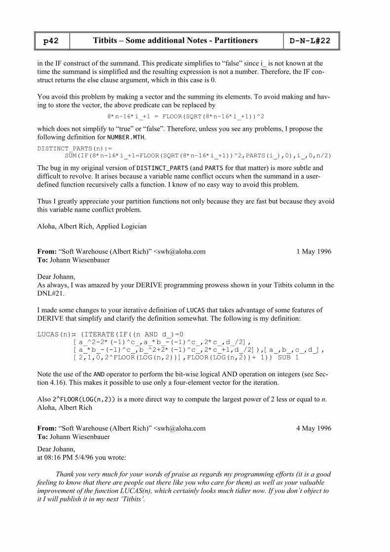
in the IF construct of the summand. This predicate simplifies to “false” since i_ is not known at the time the summand is simplified and the resulting expression is not a number. Therefore, the IF con-struct returns the else clause argument, which in this case is 0. You avoid this problem by making a vector and the summing its elements. To avoid making and hav-ing to store the vector, the above predicate can be replaced by

8*n–16*i_+1 = FLOOR(SQRT(8*n–16*i_+1))^2 which does not simplify to “true” or “false”. Therefore, unless you see any problems, I propose the following definition for NUMBER.MTH. DISTINCT_PARTS(n):= SUM(IF(8*n-16*i_+1=FLOOR(SQRT(8*n–16*i_+1))^2,PARTS(i_),0),i_,0,n/2) The bug in my original version of DISTINCT_PARTS (and PARTS for that matter) is more subtle and difficult to revolve. It arises because a variable name conflict occurs when the summand in a user-defined function recursively calls a function. I know of no easy way to avoid this problem. Thus I greatly appreciate your partition functions not only because they are fast but because they avoid this variable name conflict problem. Aloha, Albert Rich, Applied Logician From: “Soft Warehouse (Albert Rich)” <[email protected] 1 May 1996 To: Johann Wiesenbauer Dear Johann, As always, I was amazed by your DERIVE programming prowess shown in your Titbits column in the DNL#21. I made some changes to your iterative definition of LUCAS that takes advantage of some features of DERIVE that simplify and clarify the definition somewhat. The following is my definition: LUCAS(n)≔ (ITERATE(IF((n AND d_)=0

[a_^2-2*(-1)^c_,a_*b_-(-1)^c_,2*c_,d_/2], [a_*b_-(-1)^c_,b_^2+2*(-1)^c_,2*c_+1,d_/2]),[a_,b_,c_,d_], [2,1,0,2^FLOOR(LOG(n,2))],FLOOR(LOG(n,2))+ 1)) SUB 1

Note the use of the AND operator to perform the bit-wise logical AND operation on integers (see Sec-tion 4.16). This makes it possible to use only a four-element vector for the iteration. Also 2^FLOOR(LOG(n,2)) is a more direct way to compute the largest power of 2 less or equal to n. Aloha, Albert Rich

From: “Soft Warehouse (Albert Rich)” <[email protected] 4 May 1996 To: Johann Wiesenbauer

Dear Johann, at 08:16 PM 5/4/96 you wrote:

Thank you very much for your words of praise as regards my programming efforts (it is a good feeling to know that there are people out there like you who care for them) as well as your valuable improvement of the function LUCAS(n), which certainly looks much tidier now. If you don´t object to it I will publish it in my next ‘Titbits’.

D-N-L#22


p43

Please do! It is a good way to highlight DERIVE Version 3’s ability to do bitwise logical operations. Thank you also for your e-mail next to the last, although it was a bit shocking for people like me who used to think that DERIVE was relatively bugfree.

Dave and I have been “teaching” mathematics to muMATH and DERIVE for the last 18 years. In that time we have built up a test suite of over 9000 problems that DERIVE must pass before a new version is released. However, bugs will always exist in large, complex systems like DERIVE that attempt to automatically simplify any mathematical expression thrown at it. Therefore, one should never trust the results of any computer algebra system, including DERIVE. We highly recommend verifying results produced by DERIVE (e.g. substitute solutions of equations back into the original equations; differentiate antiderivatives, etc.). Well, of course I have been to used encountering bugs every now and then like e.g. LIM(x·EXP(- x^2)·INT(EXP(t^2), t, 0, x), x,inf) = 0 (cp. LIM(DIF(x·INT(EXP(t^2), t, 0, x), x)/DIF(EXP(x^2), x), x, ∞) = 1/2) Thanks for pointing out the above bug. I have fixed the problem and will send an update to Soft Warehouse Europe. Please report any other bugs in DERIVE that you encounter so they can be fixed. …but it is much harder to put with the possibility that such common functions like SUM (and supp-sedly also PRODUCT) might go haywire out of the blue after lulling the user inio a false sense of se-curity by yielding a certain amount of correct values! Maybe there is some remedy for this serious problem. Using antidifferences (like antiderivatives) is always dangerous, but I do not know of any alternative. Perhaps we could have an option to force SUM to not use the antidifference if the lower and upper limits are known. The Lorenz attractor produced with DERIVE, converted into an Acrospin file and then ani-mated. (I will show how to do this in Bonn, Josef)

p44

AC DC One

D-N-L#22

This is a second letter from Alfonso J. Población Sáez. He wrote: Dear Josef,

I send you an article which I had thought and written almost a year ago. I did not send it to you be-fore, because in fact it doesn't deal with anything especially relevant from the mathematical point of view; it is only a curiosity.Finally, I dare to send it to you.

Another question related: I was thinking (a very dangerous thing, you will see) why do not have a brief section in the newsletter in which DUG members can propose puzzles, problems (even unsolved) or mathematical recreations for which DERIVE can be applied to solve them. Some contributions pub-lished fit perfectly this idea like Conway's Game of Life, some beautiful drawings, the tennis net analysis, etc. It could be named, for example as AC DC (you know, the Amazing (or Amusing) Comer of the DERIVERs' Curiosity), or any similar thing.

Forgive me if I am completely out of order, it is only a suggestion.

With the four pages of the squaring circle article I enclose some DERIVE sheets. They are not to be included. It is only to show you how I did. Perhaps they will have better room in the diskette of the year.

Yours faithfully Alfonso J.P.S.

This is a great idea. As you can see, we have the AC DC section. We will start with your ap-proximations of squaring the circle. I could imagine that students will like your paper and will be eager to find the solutions. Josef

Some Approximazions to Square the Circle Alfonso J. Población Sáez, Valladolid, Spain

INTRODUCTION

Recreational Mathematics are generally considered only as an entertainment to kill free time. However, sometimes a lot of puzzles and challenging problems become interesting and it is necessary to apply relevant results to solve them.

One of the most popular problems since the Greeks has been the squaring of a given circle. In 1882 Ferdinand Lindemann proved by algebraical methods that this question has no solution because π is transcendent and hence is not constructible. But a great deal of people lent us some beautiful and ingenious approximations. In this brief article I have gathered four of them (from [2], [4] and [6]) in order to find ist accuracy using DERIVE. Although it is only a recreation, perhaps someone could use them as easy exercises in analytic geometry or to introduce some aspects of a part of the mathematics usually forgotten: the History of Mathematics and the evolution of the problems (see [1] and [3] for further details in this sense). So, if you have some spare time, try to answer the questions proposed!

THE PROBLEM

To square a circle consists in constructing a square having the same area as a given arbitrary cir-cle, using only straightedge and compass. This last condition means that we can only do these things: to choose points in the plane, to draw a straight line passing through two points, to draw circles of a given center and radius and to find intersection points of lines, circumferences and lines and circum-ferences.

D-N-L#22

AC DC One

p45

HOW TO USE DERIVE

Use it as you like. I have defined some functions to automate the drawings and to find the alge-braic resulats, for example:

SEGM(x,y):= to plot segments [x, y] in connected mode, MID(x,y):= to give the midpoint of a segment [x,y], EC_LINE(x_,y_):= to find the equation of a line passing points x_ and y_, DIST(x,y):= to calculate the distance between two points x and y.

and so on. For simplifying the constructions you can begin with a square and a circle with sides of length one unit, respectively. 1. One of the oldest approximations

The following procedure gives one of the best rational approximations to π and also one of the oldest. It was first used by a Chinese astronomer Tsu Ch´ung-Chih who lived in the 5th century (pic-ture on page 50).

Let ABCD be a given square (side length 1). Take E

such that 78

AE AD= and then F on BE verifying

.2

ABBF =

Consider the perpendicular to AB through F, giving point G. Finaly find H such that the segment FH is parallel to EG.

π can be approximated by 3 + HB.

What is the very known rational value and how many digits are equal to π?

2. How wrong was Hobbes? Thomas Hobbes (1588-1679) (picture on page 50) was mainly a philosopher (remember his

‘homo homini lupus’) but when he was 67 he took an interest about mathematics. He criticized those who applied algebraic methods to geometry, like John Wallis. Both of them were involved in a hard and long dispute. Hobbes found a dozen methods to square the circle. Here is one of the best in which you can use analytic geometry, in spite of Hobbes.

Starting again with a given square, draw circular arcs AC (center D) and BD (center A). F is such that arc CF = 0.5⋅CE. Then take the distance from F to segment CD and obtain G so that FG is equal to that distance and parallel to side BC.

Draw line EG and find H = EG ∩ BC.

Hobbes assured that the circumference contains the arc CE twelve times and that CE = CH, and so π is approximately 6⋅CH.

How wrong was Hobbes?

p46

S. Biryukov: Clear Function Parameters Representation

D-N-L#22

Clear Function Parameters Representation

Sergey V. Biryukov, Moscow, Russia

This report is about clear function parameters representation & ode_appr.mth extension. EULER() function which has only 1st order accuracy was included in ode_appr.mth for educational purposes. I think that some purposes require this function extension to the system of ODEs and modification to the 2nd order accuracy. Appropriate functions are defined in lines #4 and #5.

Functions with a numerous and long vector of parameters are difficult to percept. RK(r,v,v0,h,n), for instance which solves the system of ordinary differential equations has three first vector argu-ments and two last scalar ones. It would be better to arrange all data in one or several matrices and include labels for rows and/or columns. It can be done by Interface Functions which convert clear matrix-form arguments to the list of arguments, call the active function and return the result with appropriate labels. Such functions can greatly improve clearness of DERIVEed expressions and thus will be helpful for teaching. So, Interface Functions Style must be established. This report is the first attempt. Expressions #17 and #18 seem to be more alike mathematical notation than #16. Further-more they are commented and thus more suitable for teaching and using by novices in DERIVE. On the other hand #16 is more compact and clear for design and analysis by professionals.

Methods which give different orders of accuracy are compared by the example of one dimensional motion (#12 - #15, #20 - #25). #1: "=== ODE_APPR.MTH Extension for ODEs Systems === ODEAPPR1.MTH === 7 Aug 94 ===" #2: "Uses ODE_APPR.MTH & VECTOR.MTH Copyright (c) 1994 by Sergey V. Biryukov"

#3: [E(v,i):=ELEMENT(v,i),EE(v,i,j):=ELEMENT(v,i,j),D(v):=DIMENSION(v), D_E(v,i):=DELETE_ELEMENT(v,i)]

#4: EULER_SYS(r,v,v0,h,n):=ITERATES(v_+h·APPEND([1],LIM(r, v, v_)),v_,v0,n)

#5: EULER_2_SYS(r,v,v0,h,n):=ITERATES(v_+h·APPEND([1],LIM(r,v,v_+h/2·APPEND([1], LIM(r,v,v_)))),v_,v0,n) #6: "===== Clear System of ODEs Representation (Notation) ====="

#7: EULER_SYS_(m,p):=APPEND([VECTOR(LHS(EE(m,i,2)),i,2,D(m))], EULER_SYS(VECTOR(RHS(EE(m,i,1)),i,3,D(m)),VECTOR(LHS(EE(m,i,2)),i,2,D(m)), VECTOR(RHS(EE(m,i,2)),i,2, D(m)),EE(p,2,1),EE(p,2,2)))

#8: EULER_2_SYS_(m,p):=APPEND([VECTOR(LHS(EE(m,i,2)),i,2,D(m))], EULER_2_SYS(VECTOR(RHS(EE(m,i,1)),i,3,D(m)),VECTOR(LHS(EE(m,i,2)),i,2,D(m)), VECTOR(RHS(EE(m,i,2)),i,2,D(m)),EE(p,2,1),EE(p,2,2)))

#9: RK_(m,p):=APPEND([VECTOR(LHS(EE(m,i,2)),i,2,D(m))], RK(VECTOR(RHS(EE(m,i,1)),i,3,D(m)),VECTOR(LHS(EE(m,i,2)),i,2,D(m)), VECTOR(RHS(EE(m,i,2)),i,2,D(m)),EE(p,2,1),EE(p,2,2)))

#10: [E2C_(m,i,j):=D_E(EXTRACT_2_COLUMNS(m,i,j),1), "Delete 1st Row & Extract 2 Columns"] #11: ""

D-N-L#22

S. Biryukov: Clear Function Parameters Representation

p47

#12: "====== Example: One Dimensional Motion ===================" #13: "t - time, v - velocity, x - coordinate, h - time step, n - number of steps, g - acceleration of gravity " #14: "System: dv/dt=-g, dx/dt=v; Initials: t=0, v=100, x=0; Method_Parameters: time_step=1, 3 steps"

#15: g ≔ 9.81

p48

The TI-92 Corner: The CHAOS Game

D-N-L#22

The CHAOS GAME on the TI-92 (by Larry Gilligan a.o.)

In the last DNL I put L.Gilligan's, J.Rose's and N.Rich's book "Mastering the TI-92" on our book shelf. In the meanwhile I had the occasion to work with this book and I can highly rec-ommend it to you all. You will find a lot of tricks and examples how to use the TI-92. Do you know how to create you own tool bars with customized pull down menus? I know because I’ve learned it from "Mastering". I want to show one example how to program with the TI. I had not time to ask Larrie & Co for permission but I hope they will understand my idea to do some promotion for their product. I will demnstrate how to program the well known CHAOS GAME using the TI-92. I changed the program from Mastering by adding a short dialogue for the input of the parameters which are constant in the original version (the coordinates of the starting point). If you don’t know the CHAOS GAME then be patient please, in one of the next DNL's you will find a description in Maria Koth's contribution "Computer Graphics with DERIVE". Many thanks to Larry & Co in advance.

D-N-L#22

The TI-92 Corner: Integral Curves

p49

Finding Integral Curves with the TI-92

(by Josef Böhm) In the last weeks I had to teach Calculus in one of my classes. It is unevitable to solve the problem of finding an integral curve passing a given point. This was a great occasion to demonstrate the TI´s abilities.

Example 1: Let´s find the integral curve to 25' 1x

f e x= ⋅ + passing P(2|-3). You can follow the screen shots. There is a little trick which is not visible. If

you edit ∙(f,x,c) then you will obtain the antiderivative of f with respect to x and an integration constant c.

The more advanced user will try to calculate a function ic which does his work. We open the Program Editor and edit a new function called ic:

And the function does the expected work. But there is one more way to solve the problem: use Solve from the F2-Menu and build the full construction in order to solve the equation for the unknown parameter c. Example 2: 2 ;y x′ = P(3|4)

Example 3: ;atdy t edt

−= ⋅ P(4|4)

p50

The TI-92 Corner: Financial Mathematics

D-N-L#22

Classic DERIVE compared with TI-92 - DERIVE

(by Josef Böhm) The Financial Mathematics Superformula

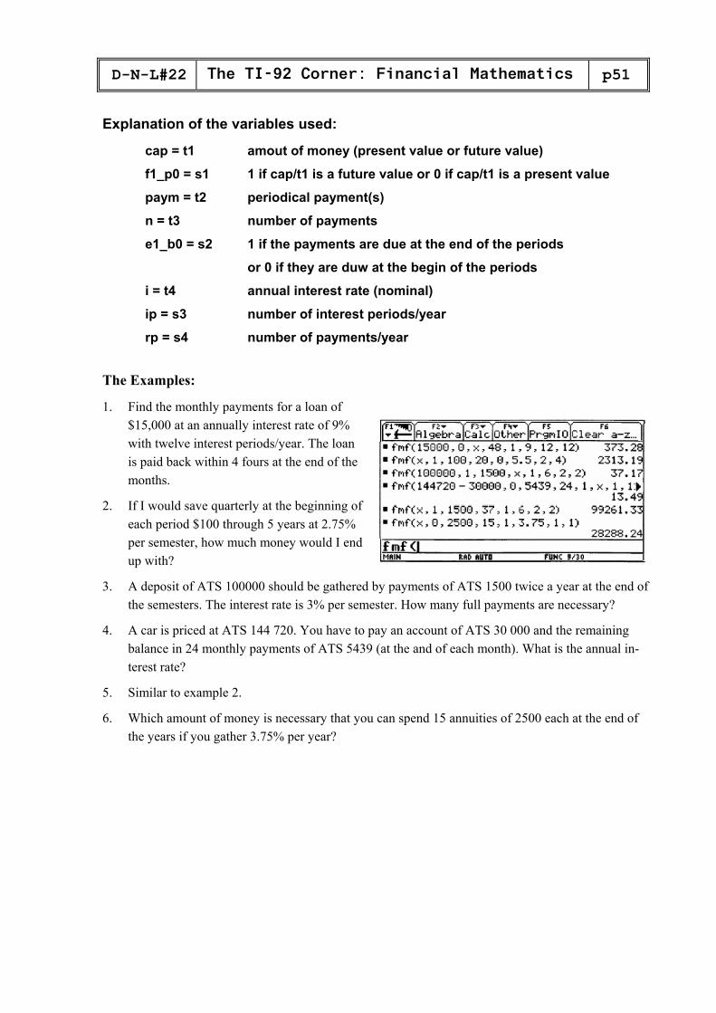
Long, long ago, in 1991, I wrote an article on financial mathematics (DNL#1,#2, 1991). I dis-cussed the use of the financial functions offered by DERIVE v.1. In the TI-92 manual I found an application (App. 15) which reminded me on these functions and gave the impact to im-prove the function presented there to find payments, future & present net values, the number of payments and the interest rate for the TI-92 and to use also DERIVE v.3´s new capabilities to build a general financial mathematical function for all purposes. See first the classic DERIVE version: (You can find the respective text for the examples on the next page.) #1: [Precision ≔ Approximate,Notation ≔ Decimal,PrecisionDigits ≔ 15] #2: InputMode ≔ Word #3: H(i,ip,rp):=(1+i/(ip·100))^(ip/rp) #4: FMF(cap,f1_p0,paym,n,e1_b0,i,ip,rp):=FLOOR(100·RHS(NSOLVE (cap=paym·(H(i,ip,rp)^n-1)/(H(i,ip,rp)-1)·(H(i,ip,rp)^ (1-e1_b0)/H(i,ip,rp)^(n·(1-f1_p0))),x,0,∞))+0.5)/100 "The examples:” FMF(15000,0,x,48,1,9,12,12)=373.28 FMF(x,1,100,20,0,5.5,2,4)=2313.19 FMF(100000,1,1500,x,1,6,2,2)=37.17 FMF(114720,0,5439,24,1,x,1,12)=13.49 FMF(x,0,2500,15,1,3.75,1,1)=28288.24 FMF(x,1,1500,37,1,6,2,2)=99261.33 And now let us try with the TI-92!: We open the Program Editor and then we edit the following program:

D-N-L#22

The TI-92 Corner: Financial Mathematics

p51

Explanation of the variables used:

cap = t1 amout of money (present value or future value)

f1_p0 = s1 1 if cap/t1 is a future value or 0 if cap/t1 is a present value

paym = t2 periodical payment(s)

n = t3 number of payments

e1_b0 = s2 1 if the payments are due at the end of the periods

or 0 if they are duw at the begin of the periods

i = t4 annual interest rate (nominal)

ip = s3 number of interest periods/year

rp = s4 number of payments/year

The Examples:

1. Find the monthly payments for a loan of $15,000 at an annually interest rate of 9% with twelve interest periods/year. The loan is paid back within 4 fours at the end of the months.

2. If I would save quarterly at the beginning of each period $100 through 5 years at 2.75% per semester, how much money would I end up with?

3. A deposit of ATS 100000 should be gathered by payments of ATS 1500 twice a year at the end of the semesters. The interest rate is 3% per semester. How many full payments are necessary?

4. A car is priced at ATS 144 720. You have to pay an account of ATS 30 000 and the remaining balance in 24 monthly payments of ATS 5439 (at the and of each month). What is the annual in-terest rate?

5. Similar to example 2.

6. Which amount of money is necessary that you can spend 15 annuities of 2500 each at the end of the years if you gather 3.75% per year?

p50


D-N-L#22

Jose Verhoosel Using DERIVE 3.11 I encountered the next problem: Using DERIVE 2.51 it is possible to solve a ⋅ [[1,2],[3,4]]=[[1,1],[2,3]]. The result is the matrix a, which fits the equation. This is not possible any more within DERIVE 3.11. Can you give me the reason or is this just another bug?

DNL: Albert Rich´s answer is: Beginning with DERIVE 3, variables can be declared integer, real, complex or nonscalar. By default variables are assumed real. Josef Lechner, Viehdorf, Austria Has anybody of you ever tried to find the general solution of a quartic using DERIVE? solve(ax^4+bx^3+cx^2+dx+e=0,x)

Modern didactics and Pedagogy?

“Teach your scholar to observe … you will soon raise his curiosity. Put the problems before him and let him solve them himself. Let him know nothing because you have told him, but because he has learned it for himself. Un-doubtely the notions of things thus acquired for oneself are clearer and much more convincing than those acqired from the teaching by others …

No, this was written by Jean-Jacques Rousseau nearly 260 years ago: Emile (1762)

Tsu Ch´ung-Chih (429 – 500) Thomas Hobbes (1588 – 1679) http://hua.umf.maine.edu/China/astronomy/tianpage/0014ZuChongzhi9296bw.html http://oregonstate.edu/instruct/phl302/philosophers/hobbes.html

Documents

THE DERIVE - NEWSLETTER #22 - Austromath · In the last time I received many interesting contributions to be published in the next DNLs. They all ... Parts of it will be the introduction