The Dependence of Protostellar Luminosity on Environment in

the Cygnus-X Star-Forming Complex

E. Kryukova1, S. T. Megeath1, J. L. Hora2, R. A. Gutermuth3, S. Bontemps4,5, K.

Kraemer6, M. Hennemann7, N. Schneider4,5, Howard A. Smith2, F. Motte7

ABSTRACT

The Cygnus-X star-forming complex is one of the most active regions of low

and high mass star formation within 2 kpc of the Sun. Using mid-infrared pho-

tometry from the IRAC and MIPS Spitzer Cygnus-X Legacy Survey, we have

identified over 1800 protostar candidates. We compare the protostellar lumi-

nosity functions of two regions within Cygnus-X: CygX-South and CygX-North.

These two clouds show distinctly different morphologies suggestive of dissimilar

star-forming environments. We find the luminosity functions of these two regions

are statistically different. Furthermore, we compare the luminosity functions of

protostars found in regions of high and low stellar density within Cygnus-X and

find that the luminosity function in regions of high stellar density is biased to

higher luminosities. In total, these observations provide further evidence that

the luminosities of protostars depend on their natal environment. We discuss the

implications this dependence has for the star formation process.

Subject headings: infrared: stars, stars: protostars, stars: formation, stars: lu-

minosity function

1Ritter Astrophysical Observatory, Department of Physics and Astronomy, University of Toledo, Toledo,

OH; megeath@physics.utoledo.edu

2Harvard-Smithsonian Center for Astrophysics, Cambridge, MA

3Department of Astronomy, University of Massachusetts, Amherst, MA

4Univ. Bordeaux, LAB, UMR 5804, F-33270, Floirac, France.

5CNRS, LAB, UMR 5804, F-33270, Floirac, France

6Institute for Scientific Research, Boston College, 140 Commonwealth Avenue, Chestnut Hill, MA 02467,

USA

7Laboratoire AIM, CEA/IRFU - CNRS/INSU - Universite Paris Diderot, Service d’Astrophysique, Bat.

709, CEA-Saclay, 91191 Gif-sur-Yvette Cedex, France

– 2 –

1. Introduction

Cygnus-X is a highly obscured area of the sky which encompasses some of the most active

regions of star formation in our galaxy known to date. It contains multiple OB associations,

including the massive Cygnus OB2 association which hosts 65 known O stars, hundreds of B

stars, and tens of thousands of low mass stars (e.g. Comeron & Pasquali 2012, Wright et al.

2010, Knodlseder 2000, Massey & Thompson 1991), as well as numerous well-studied sites

of ongoing massive star-formation including S106, W75, and DR 21 and at least 40 massive

protostars (Schneider et al. 2007, Motte et al. 2007). Cygnus-X is found near the galactic

tangent at l = 80o, and hence kinematic velocities cannot be used to estimate distances of

individual regions. Due to the large number of HII regions and star-forming regions within

Cygnus-X, it has been long debated whether Cygnus-X is a superposition of multiple clouds

along the line of sight or a single star formation complex (Reipurth & Schneider 2008, and

references therein). A recent study of the velocity structure in the CO gas by Schneider et

al. (2006) supported the view that Cygnus-X is mostly a single complex surrounding the

Cygnus OB2 association at a distance of 1.7 kpc. Further evidence for the “single complex”

view has been found in a maser parallax studies of five regions in Cygnus-X by Rygl et al.

(2012); they found that 4 out of 5 regions are at a common distance of 1.4 kpc. (We adopt

the 1.4 kpc distance from the maser parallax study, which is considered more reliable than

the 1.7 kpc distance derived from main sequence fitting).

Due to its proximity and concentration of massive star-forming regions, Cygnus-X has

emerged as a key target in studies of high mass star formation, the interaction between

molecular clouds and OB associations, and studies of star and planet formation in the OB

association environment (see for example Zapata et al. 2012, Davis et al. 2007, Wright et

al. 2012a;b). With a mass of 7.3 × 105 M⊙ (Schneider et al. 2006), about seven times that

of Orion molecular clouds (Wilson et al. 2005), Cygnus-X provides us with a nearby region

that is comparable in mass, spatial scale and luminosity to the giant star-forming regions

identified in external galaxies.

Large scale surveys of the Cygnus-X region at IR and millimeter wavelengths show

extensive populations of young stars and protostars embedded within the molecular gas.

Motte et al. (2007) surveyed the two primary molecular gas clouds in Cygnus-X: the CygX-

North cloud, which contains DR21 and W75 among other regions, and the CygX-South cloud,

which shows multi-parsec long pillars interacting with the Cyg OB2 association (Schneider et

al 2012). They discovered 129 massive cores with masses ranging from 4-950 M⊙, 42 of which

contained massive protostars. The Spitzer Cygnus-X Program (P.I. Hora) mapped a 24 deg2

field toward the complex with the IRAC and MIPS instruments onboard the Spitzer Space

Telescope. Beerer et al. (2010) studied the CygX-North cloud using the Spitzer survey data

– 3 –

and found 670 protostars and 7,249 pre-main sequence stars with disks in this region alone.

The Spitzer survey has been supplemented with near-IR photometry from the 2MASS all sky

survey and the UKIDSS galactic plane survey resulting in eight band photometry from 1.2

to 24 µm for many sources (Lucas et al. 2008). Most recently, Herschel mapped Cygnus-X in

the far-IR with the PACS and SPIRE instruments, revealing extended filamentary structures

(Hennemann et al. 2012).

In this paper, we make the first systematic survey of Spitzer-identified protostars in the

Cygnus-X region. We employ the methodology of Kryukova et al. (2012) (hereafter, KMG12),

who studied a sample of Spitzer-identified protostars in nine nearby (< 1 kpc) star-forming

regions. KMG12 used IRAC and Spitzer 24 µm photometry to identify protostars and to es-

timate their bolometric luminosity. After constructing the protostellar luminosity functions

for each of the nine clouds, they found significant differences between the protostellar lumi-

nosity functions of clouds which form high mass stars and clouds which do not. In addition,

by comparing the luminosity functions of protostars found in regions of high surface densities

of young stellar objects (YSOs) to those in regions of low YSO surface densities, KMG12

found that the luminosity function in the denser regions extended to higher luminosities than

those for lower density regions. This final result suggested that regions with higher YSO

densities preferentially form more luminous protostars, and potentially more massive stars.

Although more distant than the regions studied in KMG12, the Cygnus-X cloud com-

plex provides a much richer sample of protostars in a more extreme range of environments.

In this paper, we employ a slightly modified version of the analysis developed by KMG12

to identify protostars, determine their mid-infrared (mid-IR) and bolometric luminosities,

construct protostellar luminosity functions and correct the luminosity functions for contami-

nation. We also perform an analysis of the spatially varying incompleteness of the protostars.

Taking into account this incompleteness, we compare different regions within Cygnus-X to

search for variations in the protostellar luminosity function between clouds within the com-

plex. Furthermore, we compare regions of high and low YSO density to test whether the

protostellar luminosity function extends to higher luminosities in dense regions, as found for

Orion by KMG12. With these results, we argue that the protostellar luminosity function in

Cygnus-X depends on the environment in which the protostars form.

– 4 –

2. Protostar Identification

2.1. Near- & Mid-Infrared Photometry

The Cygnus-X complex was the target of the Cygnus-X Spitzer Legacy Survey1, which

mapped 24 deg2 of the complex with the Infrared Array Camera (IRAC, Fazio et al. 2004)

and Multiband Imaging Photometer for Spitzer (MIPS, Rieke et al. 2004) instruments on

board the Spitzer Space Telescope2. We used IRAC aperture photometry and MIPS 24 µm

point-spread function (PSF) photometry from Data Release 1 Point Source Catalog with

no alteration. The PSF photometry extraction at the MIPS 24 µm wavelength is used to

minimize source confusion due to nebulosity. However, the brightest sources are saturated

in the 24 µm image and the photometry is not available for these sources. Thus, our study

excludes the sources with the brightest m24 magnitudes in Cygnus-X.

The photometry in the five Spitzer bands is augmented by photometry at near-IR J, H,

and K-bands. This photometry is preferentially from the UKIRT Infrared Deep Sky Survey

(UKIDSS) (Lucas et al. 2008), but for sources for which UKIDSS data do not exist, we

use available photometry from the Two Micron All-Sky Survey (2MASS, Cutri et al. 2003,

Skrutskie et al. 2006).

2.2. Protostar Candidate Selection

Mid-infrared colors can be used to identify infrared young stellar objects (YSOs) by the

excess infrared emission radiated by their dusty disks and envelopes (e.g., Greene et al. 1994,

Bontemps et al. 2001, Allen et al. 2004, Megeath et al. 2004, Muzerolle et al. 2004, Whitney

et al. 2004, Robitaille et al. 2006, Harvey et al. 2007, Winston et al. 2007, Gutermuth et

al. 2009). We use the criteria of KMG12 to identify protostars in the Cygnus-X point

source catalog. These criteria are based on identification of protostars with flat and rising

spectral energy distributions (SEDs) between 4.5 and 24 µm. We use the spectral index α =

δ log(λFλ)/δ(log(λ)) calculated between 3.6 and 24 µm, to determine this slope. Following

the approach of KMG12, we search for protostars with in-falling protostellar envelopes by

identifying sources with both flat SEDs (-0.3 < α< 0.3), which correspond to flat spectrum

protostars, and rising SEDs (0.3 > α), which correspond to Class 0/I protostars (Lada

1From http://irsa.ipac.caltech.edu/data/SPITZER/Cygnus-X/

2Data delivery document can be found at http://irsa.ipac.caltech.edu/data/SPITZER/Cygnus-

X/docs/CygnusDataDelivery1.pdf

– 5 –

& Wilking 1984, Calvet et al. 1994, Winston et al. 2007, Enoch et al. 2009). KMG12

implemented this approach by converting the spectral indicies into a series of color criteria

involving the four IRAC bands and the MIPS 24 µm band. They require that all protostars

show a detection in the 24 µm band.

While most of our protostar selection criteria is the same as that of KMG12, we adjust

one set of criteria. Normally protostar candidates are selected in part by their red [3.6] -

[4.5] color; however, due to the large amount of scattered light in the 3.6 and 4.5 µm bands,

some protostars have a very red [4.5] - [24] color but a [3.6] - [4.5] color between 0.7 and

0 mag. KMG12 selected these sources by the criteria in their Equation 3. However, due

to the distance and bright nebulosity of Cygnus-X, nebulous knots may be mis-identified as

protostars by the same criteria. These knots are distinguished by their bright PAH emission

at 3.6 µm and weak emission at 4.5 µm, which results in a [3.6] - [4.5] color less than 0 mag.

We subject the sources which fit Equation 3 of KMG12 to the following additional condition:

[3.6] − [4.5] ≥ 0 (1)

which eliminates 15 likely nebulous knots with very blue [3.6] - [4.5] colors due to their

bright 3.6 µm PAH emission. In comparison, only one of the protostar candidates found in

the sample of nearby clouds by KMG12 satisfies the criteria shown in their Equation 3, but

fails the criterion in Equation 1 above.

The color-color and color-magnitude diagrams we use to identify protostar candidates

are shown in Figure 1 and Figure 2. Sources that satisfy any of the criteria in Table 1 are

considered protostar candidates. We give the number of rising and flat SED protostars,

distinguished by α > 0.3 as rising SED protostars and 0.3 > α > -0.3 as flat SED protostars,

in Table 2.

The spatial distribution of these sources is overlaid on the extinction map of the region

shown in Figure 3. Note that most of the protostar candidates are concentrated in high

extinction regions. To further minimize contamination, we require that protostar candidates

must lie in locations where the visual extinction measured toward background stars is > 3,

as determined from the extinction map shown in Figure 3. This extinction map, covering the

Spitzer-mapped region, is derived using AvMAP from Sylvain Bontemps (private communi-

cation; see Schneider et al. 2011). The resulting coverage area with AV > 3 is 21.75 deg2. For

comparison, Figure 4 shows the 13CO J = 1→0 velocity integrated intensity map also from

Schneider et al. (2011). By requiring a minimum AV , we limit the area in which we search

for protostars to regions which are known to contain molecular gas. Since protostars will be

concentrated in regions with high column densities of gas while contaminating objects will

– 6 –

be more evenly spread throughout the sky, this has the advantage of reducing the amount

of contamination.

Table 1: Number of protostar candidates identified by selection

criteria

Equation Selection Criteria Colors Number Number

AV > 3

(1)a, (2)a [4.5]-[24], [3.6]-[4.5] 1781 1611

(3)a, (1)b [4.5]-[24], [5.8]-[8.0], [3.6]-[4.5] 127 111

(4)a,c [5.8]-[24], [3.6]-[5.8] 179 143

(5)a,d [8.0]-[24], [3.6]-[8.0] 170 142

a Criteria given from KMG12.b Criteria from KMG12 that were modified in this workc Only for sources without 4.5 µm detections.d Only for sources without 4.5 and 5.8 µm detections.

All protostar candidates selected using these criteria must also satisfy a 24 µm mag-

nitude cutoff. This cutoff is imposed to eliminate galaxies with colors similar to YSOs,

but which have fainter m24 mag (Megeath et al. 2009). We determine the m24 magnitude

cutoff using the method of KMG12. In this method, we first determine the spatial density

of galaxies with colors similar to protostars using the point source catalog from the Spitzer

Wide-Area Infrared Extragalactic Survey Legacy Program (SWIRE, Lonsdale et al. 2003)3.

We compare the distribution of m24 for the Cygnus-X protostar candidates in the region

where AV > 3 and for the SWIRE sample which satisfies the protostar candidate selection

criteria. The SWIRE histogram is scaled up to account for the larger angular extent of the

AV > 3 region. We do not apply reddening to the SWIRE sample making our cutoff more

conservative than necessary. However, for an AV > 3 the extinction at 24 µm is only A24 >

0.3 (Chapman & Mundy 2009), hence extinction may not have a large effect on the cutoff.

The m24 cutoff of m24 = 7.5 mag is shown in Figures 2 and 5. Below this m24 cutoff we

find 2007 protostar candidates projected on regions with AV > 3. In comparison, there are

77.7 SWIRE galaxies that fit our protostar selection criteria colors after accounting for the

larger angular extent of the AV > 3 area, resulting in a contamination rate of 4.2%. Another

potential source of contamination are HII regions and reflection nebulosity in the molecu-

3We used the 4.2 deg2 Elais-N2 field from http://swire.ipac.caltech.edu/swire/swire.html

– 7 –

lar cloud complex. Because we require that the sources in our catalog be point sources in

the IRAC and MIPS bands, these would have to be very ultracompact HII regions or very

small reflection nebulae with sizes ≤ 7000 A.U., the spatial resolution at the distance of

Cygnus-X. Future, higher resolution near-IR observations may provide an effective means

of further eliminating such compact HII regions and nebulae from our sample of protostars.

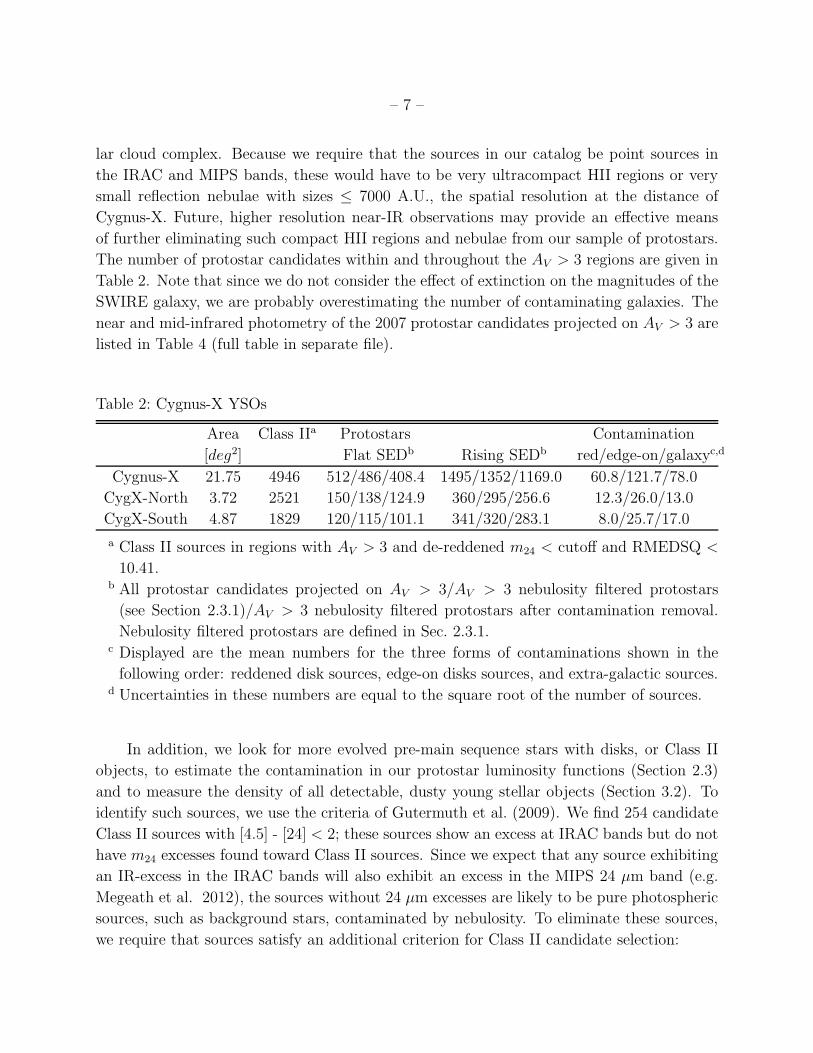
The number of protostar candidates within and throughout the AV > 3 regions are given in

Table 2. Note that since we do not consider the effect of extinction on the magnitudes of the

SWIRE galaxy, we are probably overestimating the number of contaminating galaxies. The

near and mid-infrared photometry of the 2007 protostar candidates projected on AV > 3 are

listed in Table 4 (full table in separate file).

Table 2: Cygnus-X YSOs

Area Class IIa Protostars Contamination

[deg2] Flat SEDb Rising SEDb red/edge-on/galaxyc,d

Cygnus-X 21.75 4946 512/486/408.4 1495/1352/1169.0 60.8/121.7/78.0

CygX-North 3.72 2521 150/138/124.9 360/295/256.6 12.3/26.0/13.0

CygX-South 4.87 1829 120/115/101.1 341/320/283.1 8.0/25.7/17.0

a Class II sources in regions with AV > 3 and de-reddened m24 < cutoff and RMEDSQ <

10.41.b All protostar candidates projected on AV > 3/AV > 3 nebulosity filtered protostars

(see Section 2.3.1)/AV > 3 nebulosity filtered protostars after contamination removal.

Nebulosity filtered protostars are defined in Sec. 2.3.1.c Displayed are the mean numbers for the three forms of contaminations shown in the

following order: reddened disk sources, edge-on disks sources, and extra-galactic sources.d Uncertainties in these numbers are equal to the square root of the number of sources.

In addition, we look for more evolved pre-main sequence stars with disks, or Class II

objects, to estimate the contamination in our protostar luminosity functions (Section 2.3)

and to measure the density of all detectable, dusty young stellar objects (Section 3.2). To

identify such sources, we use the criteria of Gutermuth et al. (2009). We find 254 candidate

Class II sources with [4.5] - [24] < 2; these sources show an excess at IRAC bands but do not

have m24 excesses found toward Class II sources. Since we expect that any source exhibiting

an IR-excess in the IRAC bands will also exhibit an excess in the MIPS 24 µm band (e.g.

Megeath et al. 2012), the sources without 24 µm excesses are likely to be pure photospheric

sources, such as background stars, contaminated by nebulosity. To eliminate these sources,

we require that sources satisfy an additional criterion for Class II candidate selection:

– 8 –

[4.5] − [24] ≥ 2 (2)

which all Class II sources with detections at 4.5 and 24 µm must satisfy. We eliminate these

potential contaminants from our Class II sample. The Class II sources are also shown in

Figures 1 and 2. Listed in Table 2 are the number of Class II sources we find in regions of

AV > 3 as well as the number of protostar candidates in these regions.

2.3. Building the Protostellar Luminosity Function

To determine the protostellar luminosity function in Cygnus-X, we must first estimate

bolometric luminosities for each of our protostar candidates. Since the majority of the flux

from a protostar is emitted at wavelengths longward of the photometry bands available in

this study, we use the relationship between mid-IR luminosity (calculated from 1-24 µm),

the SED slope, and the bolometric luminosity developed by KMG12. This relationship was

determined using a sample of low- to intermediate-luminosity protostars (0.03 L⊙ to 19.6

L⊙). We calculate the mid-IR luminosity of the protostar candidates using Equation 6 from

KMG12. Once determined, we use the mid-IR luminosity and SED slope with Equations

7 and 8 from KMG12 to find the bolometric luminosity. The median slope of Cygnus-X

protostar candidates is 0.75, and 90% of Cygnus-X protostar candidates have slopes less

than 1.57.

The range of luminosity we find for the protostar candidates in Cygnus-X extends from

0.1 L⊙ to 3370 L⊙, with 89% of the protostar candidates having luminosities below 19.6 L⊙.

Objects with luminosities > 3000 L⊙ are missing due to saturation in the 24 µm band. Since

the luminosity depends both on the flux in all the 3.6 through 24 µm bands and the slope

of the SED, a definite saturation luminosity cannot be established. Future work analyzing

Herschel and WISE data may establish the number of luminous sources missed in the Spitzer

survey. Motte et al. (2007) find the presence of 25 massive protostars in their study of the

Cygnus-X; we expect the number of missing sources to be of this order of magnitude.

The systematic uncertainties in the luminosities determined by this method are de-

scribed by KMG12; they find the log of the ratio of the well-determined bolometric lumi-

nosity to the estimated bolometric luminosity has a mean value of 0.06 with a standard

deviation of 0.35. We expect that neither the systematic uncertainties nor the uncertainties

from the fluxes used in determining LMIR should affect the gross properties of the displayed

luminosity functions. Furthermore, even if systematic uncertainties affect the conversion of

the measured LMIR into bolometric luminosities, such uncertainties would presumably affect

– 9 –

all sources in the same way, and thereby leave the comparisons unaffected. The bolometric

luminosities of the protostar candidates are listed in Table 4 (full table in separate file).

2.3.1. Completeness at m24

The derived protostellar luminosity function is affected by spatially varying completeness

(KMG12, Megeath et al. 2012). Since we require of our protostars a detection in m24, we

are primarily concerned with the completeness in this band, and in comparison to the 3.6

and 4.5 µm bands the nebulosity will have the most effect at 24 µm. We follow the approach

of Megeath et al. (2012) to determine the completeness as a function of the fluctuations due

to nebulosity and confusion from other point sources.

The completeness in the Spitzer images is spatially varying primarily due to the bright,

highly structured nebulosity found in Spitzer images of star-forming regions. Instead of

measuring the completeness independently at each position, we measure the completeness as

a function of source magnitude and the RMEDSQ, a measure of the fluctuations in the signal

due to nebulosity and neighboring point sources in an annulus immediately surrounding a

point source. Megeath et al. (2012) define RMEDSQ =√

median[(Sij − median(Sij))2],

where Sij is the signal in DN s−1 pix−1 at a given pixel position i,j. The median values are

determined for an annulus centered on each source; this annulus typically extends from 6 to

11 pixels but is increased for more luminous sources (Megeath et al. 2012). Thus, we first

assign to each of our sources a RMEDSQ.

To measure the completeness to point sources as a function of the RMEDSQ, we create

an overlay of PSFs arranged in a 3 × 3 grid and add it to the Spitzer 24 µm mosaic. The

grid is created by using the MIPS 24 µm PSF scaled to varying magnitudes, including m24

= 3.125, 3.625, 4.125, 4.625, 5.125, 5.625, 6.125, 6.625, and 7.125, spaced 25 pixels from

one another. This grid is then repeatedly added to the Cygnus-X 24 µm image at intervals

of 151 pixels across the mosaic so that the entire image is covered by the repeating grid.

The mosaic has a pixel size of 1.”2. We use PhotVis (Gutermuth et al. 2008) to find all the

24 µm point sources in the mosaic and perform aperture photometry on the sources. We

consider an input PSF recovered if a point source is found within 2.”5 of the input PSF’s

position with a magnitude within 0.25 mag of the input PSF’s magnitude. The RMEDSQ

is determined around each of the input PSFs. For each input magnitude, these sources are

then binned by RMEDSQ. Figure 6 shows the fraction of recovered sources as a function of

the log(RMEDSQ) for each of the input magnitudes.

To mitigate the incompleteness in extended regions of bright nebulosity and extreme

– 10 –

source crowding, we first measure the incompleteness in the region surrounding each proto-

star. To do so, we use the average RMEDSQ value of YSOs (protostar candidates projected

on AV > 3 regions and Class II sources) within a critical distance, Dc = 0.62 pc (see Section

3.2), of each protostar, which we denote <RMEDSQ>Dc value for that protostar. Using the

mean RMEDSQ value for nearby YSOs provides a more representative measurement of the

typical fluctuations in the regions surrounding each protostar than using only the RMEDSQ

value for the protostar. The <RMEDSQ>Dc value is listed for each protostar candidate in

Table 4 (full table in separate file).

In Figure 7, we show the <RMEDSQ>Dc value vs. bolometric luminosity for each

protostar candidate in Cygnus-X, CygX-North, and CygX-South. This figure shows that

incompleteness can result in a clear bias in our determination of the luminosity functions in

that luminous protostars can be found in regions with high RMEDSQ where lower luminosity

protostars cannot be detected. To eliminate this bias, we filter out sources with either high

values of RMEDSQ or low values of luminosity. We first determine a cutoff RMEDSQ value

such that 90% of the YSOs, including other protostar candidates and Class II sources within

Dc = 0.62 pc of a protostar candidate, have <RMEDSQ>Dc values below this cutoff; the

value of the cutoff is 10.41. Using the curves from Figure 6, we interpolate between curves

to find a limiting m24 that corresponds to a 90% completeness at the cutoff RMEDSQ value.

The resulting limiting m24 is 5.07 mag. The corresponding limiting m24 is converted to a

luminosity using Equation 6 of KMG12 assuming the entire mid-IR luminosity is given by the

24 µm flux and assuming an SED slope larger than that of 90% of the protostar candidates

in Cygnus-X. The corresponding cutoff luminosity is 2.16 L⊙. Thus, we find that we are 90%

complete at a luminosity cutoff of Lcut = 2.16 L⊙ and an <RMEDSQ>Dc = 10.41. Most of

the protostars will be in regions that have smaller <RMEDSQ>Dc values and hence higher

levels of completeness at 2.16 L⊙.

The RMEDSQ cutoff and Lcut are also shown in Figure 7. There are 1838 protostar

candidates with <RMEDSQ>Dc values less than 10.41; we refer to these protostars as the

“nebulosity filtered” sample in the remaining text. We only use sources below this cutoff

and luminosity greater than Lcut = 2.16 L⊙ when comparing the luminosity functions. The

regions around the sample nebulosity filtered protostars are 99.7% complete at Lcut.

2.3.2. Protostellar Luminosity Functions

In Figure 8, we show the luminosity functions of the protostar candidates. We display

the luminosity functions for the entire region, the CygX-North region, and the CygX-South

region, as defined by Schneider et al. (2006) (see Section 3.0). To probe the differences be-

– 11 –

tween the various star-forming environments, we compare luminosity functions of protostars

in different regions. However, there are yet multiple sources of contamination which are

not eradicated by the protostar selection criteria of Section 2.2, which include edge-on disks

(Crapsi et al. 2008), highly reddened Class II sources where the extinction results in a rising

SED (Evans et al. 2009, McClure et al. 2010), and galaxies with m24 brighter than our m24

cutoff.

For each type of contamination, we generate multiple realizations of their luminosity

functions using the Monte Carlo method described in Section 4 of KMG12. For sources with

edge-on disks, the ratio of edge-on disks to all Class II objects and the luminosities of the

edge-on disks sources are determined from a sample of likely edge-on disks in the Cep OB3b

cluster as described by KMG12. To estimate the number of edge-on disks, we multiple this

ratio by the number of Class II sources with <RMEDSQ>Dc < 10.41. The highly reddened

Class II sources are identified using the same technique as in KMG12, but utilizing a fiducial

sample of low-AV Class II sources with <RMEDSQ>Dc < 10.41 from Cygnus-X. These are

reddened using the extinctions toward the sample of protostars and YSOs with AV > 3

and <RMEDSQ>Dc < 10.4 (see KMG12 for the details of this process). The method of

estimating galaxy contamination is unchanged from KMG12 and utilizes the same SWIRE

sample as a galaxy sample. The methods for determining the luminosity functions of the

edge-on sources and highly reddened Class II sources require us to use the number of Class

II sources with <RMEDSQ>Dc below 10.41.

For each Monte Carlo realization, we determine a sample of contaminants as described

by KMG12. We calculate the luminosity of each contaminant using the mid-IR luminosity

and SED slope; this may not be the actual luminosity of the contaminating source, but

instead the luminosity we would assign to the source given its mid-IR photometry. We then

remove a source from the protostar luminosity function which has the closest luminosity to

the contaminant, requiring that the difference is less than 0.2 dex. If no protostar candidate

has such a luminosity, then no source is removed. We repeat this process for each of the 1000

realizations. We stress that we are not identifying protostar candidates as contamination and

removing them, instead we predict the luminosities for ensembles of contaminating sources

as generated by the Monte Carlo code and remove those luminosities from the protostellar

luminosity function. The resulting mean luminosity distributions of edge-on disks, galaxies,

and reddened Class II sources found over the 1000 trials of the Monte Carlo code are shown

in Figure 8, along with the luminosity function of the protostar candidates. The protostellar

luminosity functions with the contamination removed are shown in Figure 9; these have been

averaged over the 1000 trials. The luminosity functions for the total region, the CygX-North

region, and the CygX-South region are shown; the above procedure was run for each of these

regions independently. The m24 cutoff, along with the number of contaminants, protostar

– 12 –

candidates, Class II sources with AV > 3, and flat and rising SED protostars are listed in

Table 2.

We find that the contaminants account for only 14.2% of our total 1838 protostar can-

didates. The most common type of contamination is due to edge-on disk sources. However,

because Cygnus-X is both in the Galactic plane and a more distant cloud than those stud-

ied in KMG12, there may be additional sources of Galactic contamination such as more

distant star-forming regions or more evolved stars. We have attempted to minimize that

contamination by only including protostar candidates projected on regions of AV > 3.

3. Protostellar Environment and Luminosity

The distribution of protostars and their relationship to the distribution of molecular

gas, as delineated by the AV map or the 13CO velocity integrated intensity map, is shown in

Figures 3 and 4. The locations of the most luminous protostar candidates are shown circled

in red. These maps show that the Cygnus-X complex is dominated by two cloud complexes,

the CygX-North and CygX-South complex. Schneider et al. (2006) argued that CygX-North

and CygX-South are at a similar distance as the Cyg OB2 association and that Cygnus-X is

mostly a coherent complex rather than a superposition of clouds at varying distances. More

recently, Rygl et al. (2012) found that DR 21, DR 20, W75N, and IRAS 20290+4052, all

within the northern cloud, are consistent with a distance of 1.4 kpc, but AFGL 2591, which

is located within our boundary for CygX-South, is at a distance of 3.33±0.11 kpc. However,

given the evidence that CygX-South is interacting with the Cyg OB2 association, we will

assume that the CygX-North and CygX-South clouds are at 1.4 kpc, although there is some

contamination with more distant regions (Schneider et al. 2012).

The CygX-North and CygX-South molecular clouds exhibit different morphologies in

their mid-IR emission and in the distribution of protostars relative to the molecular gas.

Maps of the mid-IR emission with the position of the protostars overlaid are shown in

Figures 10 and 11. We see in Figure 3 and Figure 4 that within our chosen boundary

for CygX-North, the spatial distribution of protostars tends to follow the cloud structure

apparent in both the AV map and 13CO map. The central cloud is filamentary in structure

containing rich, multi-parsec chains of protostar candidates. These are particularly apparent

in DR 21, DR 22, DR 23 and W75; the filament containing DR21 and W75 is perhaps the

most active star-forming region in the CygX-North (Beerer et al. 2010, Schneider et al.

2010). Although there are UV illuminated features on the side of the cloud facing Cyg OB2

(Schneider et al. 2006), the DR21/W75 filament is not associated with extended, bright IR

nebulosity. The lack of nebulosity indicates that this filament is not being directly illuminated

– 13 –

by the Cyg OB2 association. We also do not find an excess of luminous protostar candidates

on the edge of the CygX-North cloud closest to Cyg OB2; although, the most luminous

protostar candidates are primarily found in the half of the CygX-North region closest to

Cyg OB2. This suggests that much of the star formation in the CygX-North is not being

directly influenced by the UV radiation and winds from Cyg OB2.

In CygX-South, the protostars tend to be located toward the outer parts of the cloud

on both maps, with fewer protostar candidates being found toward the center of the cloud.

Compared to CygX-North, the cloud morphology in CygX-South is less dominated by fila-

mentary structures. The CygX-South appears to be more strongly interacting with the Cyg

OB2 association and contains prominent pillars extending towards and illuminated by Cyg

OB2, which is 40 pc north of the heads of the pillars (Figure 11, Schneider et al. 2012). The

part of the CygX-South region facing Cyg OB2 has an abundance of protostar candidates. In

contrast, there are relatively few protostar candidates located in some of the densest regions

of the 13CO map in the central and southern parts of CygX-South. The concentration of

protostars near Cyg-OB2 suggest that a wave of star formation is being driven into CygX-

South by the direct compression of the cloud surfaces by Cyg OB2. This direct compression

may be result from the photoevaporation of the cloud surfaces by the UV field from Cyg

OB2 (e.g. Megeath & Wilson 1997, Deharveng et al. 2010). The different spatial distribu-

tions of protostars and gas in the CygX-South and CygX-North regions are evidence that

both radiatively triggered and a more spontaneous star formation are currently operating in

Cygnus-X.

3.1. Protostellar Luminosity Functions of CygX-North and CygX-South:

Evidence for Variations

In the previous section, we showed that the spatial distribution of protostars and the

morphologies of their parental clouds appear to be different in the CygX-North and CygX-

South. Here we test whether the protostellar luminosity functions of these sub-regions are

similar.

We first comment on the shape of the Cygnus-X, CygX-North, and CygX-South lumi-

nosity functions of the nebulosity filtered protostars (Figure 9). None of these luminosity

functions has a peak above Lcut = 2.16 L⊙, but rather in each case, the luminosity func-

tions increase toward lower luminosity, though the Cygnus-X and CygX-North luminosity

functions rise more steeply than the CygX-South luminosity function. The CygX-North lumi-

nosity function has an excess of sources near 100 L⊙ relative to the Cygnus-X or CygX-South

luminosity functions. Above Lcut = 2.16, the Cygnus-X luminosity function has a maximum

– 14 –

luminosity of 3370 L⊙ (close to the saturation limit), a median value of 6.8+8.4−3.8 L⊙, a mean

value of 30.5+37.8−16.9 L⊙ and standard deviation of 144.2+178.6

−79.8 L⊙. The uncertainties for the

mean and median are due to those in the determination of Lbol, where the standard devia-

tion of the log of the luminosity integrated over the SED of sources with far-IR photometry

over that estimated from LMIR (i.e. log [Lbol(SED)/Lbol(MIR)]) is 0.35. The CygX-North

luminosity function has a maximum luminosity of 280+347−155 L⊙, a median of 7.3+9.0

−4.0 L⊙, a

mean of 26.6+33.0−14.7 L⊙, and standard deviation of 46.2+57.2

−25.6 L⊙. In CygX-South, the maximum

luminosity is 276+342−153 L⊙, with a median of 7.4+9.2

−4.1 L⊙, a mean of 19.0+23.5−10.5 L⊙, and standard

deviation of 34.9+43.2−19.3 L⊙. The CygX-North and CygX-South regions have similar numbers of

protostars, with CygX-North containing 157 nebulosity filtered protostars and CygX-South

containing 169 nebulosity filtered protostars with Lcut > 2.61 L⊙.

A statistical comparison using a two sample Kolmogorov-Smirnov (K-S) test allows us

to determine the probability that any two luminosity functions are from the same parent

distribution. To take into account uncertainties in the correction for contamination, we use

an ensemble of 1000 distributions of each luminosity function, each of which is a realization

from the Monte Carlo method used to estimate contamination. We perform the K-S test 1000

times between realization 1 from luminosity function A with realization 1 from luminosity

function B, and realization 2 from luminosity function A with realization 2 from luminosity

function B, and so on (see KMG12). We then take the median probability from the 1000

realizations. Only nebulosity filtered sources above Lcut are used in the test.

We first compare the luminosity function of the entire Cygnus-X sample with both

the individual CygX-North and CygX-South luminosity functions. The median probabili-

ties from the K-S test comparing the CygX-North and CygX-South luminosity function to

the entire Cygnus-X cloud luminosity function are listed in Table 3. These results indicate

that the CygX-North luminosity function is not drawn from the same parent distribution

as the entire Cygnus-X cloud luminosity function. In comparison, the Cygnus-X luminosity

function and CygX-South luminosity function are likely drawn from the same parent distri-

bution. Comparing the CygX-North and CygX-South luminosity functions, we find that the

protostellar luminosity function of CygX-North has a median probability log(prob) = -7.47

of being from the same parent distribution as the luminosity function of the protostars in

CygX-South (Table 3). If we increase Lcut to 3 L⊙, the probability decreases to log(prob) =

-9.4 that CygX-North and CygX-South are drawn from the same distribution.

Could differences we observe be an artifact resulting from the superposition of multiple

star-forming regions at different distances? Our determination of the protostellar luminosity

adopts a single distance for each of our samples; the presence of multiple distances may result

in a shift of the luminosity function or a broader spread of luminosities. However, Schneider

– 15 –

et al. (2006) argue on the basis of their 13CO data that the CygX-North and CygX-South

are coherent cloud regions and that they are both associated with Cygnus-X. The degree of

contamination from larger distances is likely small, particularly if we limit ourselves to the

CygX-North and CygX-South regions. The maser parallaxes of Rygl et al. (2012) show only

one out of five regions is a background region located at a larger distance of 3 kpc. This

more distant region, AFGL 2591, is spatially enclosed in the CygX-South region, but is at

a distance approximately twice that of the CygX-South region (Schneider et al. 2006). We

do not include this source in our protostar candidate list because it is saturated at m24, and

thus it does not affect the CygX-South luminosity function.

Furthermore, a small difference in distances for CygX-North and CygX-South is unlikely

to affect our comparison. Even if CygX-North and CygX-South are on the opposite sides

of the Cyg OB2 association, they would be separated by 100 pc, resulting in a small shift

in log(L [L⊙]) of 0.06 (Schneider et al. 2006). Thus, because the evidence favors the CygX-

North and CygX-South regions as containing coherent clouds at nearly the same distance, we

conclude that the differences in the luminosity functions between these regions are very likely

to be real. Over the entire Cygnus-X region, there may be a higher degree of contamination

from protostars at different distances; this may potentially contribute to the dissimilarity

between the Cygnus-X and CygX-North luminosity functions. Hence, we are not as confident

of differences between the CygX-North and the Cygnus-X regions.

Table 3: K-S Test probabilities

Region CygX-North CygX-South High/Low Density HMSFCa LMSFCb

Cygnus-X -9.93c 0.9085 -3.19c 0.6343 0.0200

CygX-North - -7.47c -5.42c -5.88c -4.33c

CygX-South -7.47c - 0.0135 0.8123 0.0111

a HMSFC are high mass star-forming clouds, see Sec. 3.3.b LMSFC are low mass star-forming clouds, see Sec. 3.3.c Given as log(prob).

3.2. Protostellar Luminosity and Stellar Density

KMG12 found a dependence of the protostellar luminosity function on the density of

YSOs in the Orion molecular clouds, with the luminosity function being biased to higher

luminosities in regions of high stellar density. We now repeat this analysis for the Cygnus-X

region to see if the same dependence is apparent. To sort protostars by the local surface

– 16 –

density of YSOs, we use the nearest-neighbor distance. This distance is found to the 4th

nearest YSO, which we designate “nn4 distance” following the approach of KMG12. We

include both the nebulosity filtered protostar candidates projected on AV > 3 regions and

Class II sources without AV or RMEDSQ cutoffs as YSOs. Figure 12 shows the distribution

of bolometric luminosity vs. nn4 distance for the entire cloud sample, CygX-North sample,

and CygX-South sample. Similar to what KMG12 found for nearby high mass star-forming

clouds, we find that in each sample the maximum nn4 distance of the protostar candidates

tends to decrease with increasing luminosity (except for the most luminous protostar can-

didate in the Cygnus-X sample). This trend is particularly pronounced in the CygX-North

region. At low luminosities near our completeness limit, Lcut = 2.16 L⊙, we find protostar

candidates at both large and small nn4 distances. The spatial distribution of the protostars

in these two environments are shown in Figures 3 and 4, with the blue and green symbols

marking the positions of protostars in low and high stellar density environments, respec-

tively. Note this analysis does not account for the saturated protostars missing from our

sample which will be more luminous than the sample of observed protostars.

We now seek to compare luminosity functions of protostars in high and low stellar

density environments. To determine if a protostar candidate is in a high or low stellar

density environment, we use the median nn4 distance, denoted Dc, for the Cygnus-X cloud

nebulosity filtered sample. This provides an equal number of protostar candidates in high

and low stellar density regions in Cygnus-X, which is optimal for statistical comparisons

between the two samples. We find Dc = 0.62 pc, which is equivalent to a surface density of

4.15 YSOs pc−2. In comparison, this number is less dense than the definitions of a cluster

given by Carpenter (2000), Gutermuth et al. (2009), and Bressert et al. (2010), even though

Carpenter (2000) and Gutermuth et al. (2009) find that approximately half of YSOs are

found in clusters. The Dc used for Cygnus-X is also larger than the Dc used for nearby

molecular clouds by KMG12 (0.08 to 0.4 pc). However, the Cygnus-X region is more distant

than the regions in the above studies and hence is more incomplete to lower mass Class II

objects and protostars. For this reason, a larger value of Dc is appropriate for Cygnus-X.

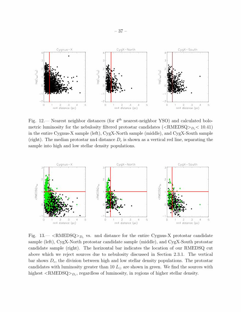
In Figure 13, we show the log(<RMEDSQ>Dc) deviation as a function of nn4 dis-

tance, with the sources having luminosities above 10 L⊙ marked. We find the most lu-

minous protostars tend to be in high stellar density environments with high values of

<RMEDSQ>Dc . These plots also show that the regions where nn4 < Dc have preferentially

higher <RMEDSQ>Dc values. This demonstrates why we must only consider nebulosity

filtered protostars even though many of the higher luminosity sources are excluded from the

analysis. By ignoring regions where the <RMEDSQ>Dc is above our adopted threshold, our

sample of protostars in the remaining regions is 90% complete at our luminosity cutoff, Lcut

= 2.61 L⊙.

– 17 –

We note that although there are equal number of protostars in high and low stellar

density regions for the entire sample, that is not true for the individual clouds. CygX-North

has a notably larger percentage of nebulosity filtered protostar candidates with luminosities

above Lcut in high stellar density environments (67.3%) as does the CygX-South region

(60.4%). Furthermore, the percentage of sources in high stellar density regions increase for

more luminous sources. In CygX-North, 77.2% of the nebulosity filtered protostar candidates

with luminosity greater than 10 L⊙ are in high stellar density environments, in CygX-

South this number is 69.6%, and across the entire Cygnus-X sample, we find 68.4% of high

luminosity protostars in high stellar density environments. This shows that the sources with

luminosities exceeding 10 L⊙ are more likely to be in crowded regions than lower luminosity

sources.

We compare the luminosity functions of the protostars in higher stellar density environ-

ments with luminosity functions of protostars in lower stellar density environments in Figure

14. We see an excess of high luminosity sources in high stellar density regions above Lcut in

each of the Cygnus-X, CygX-North, and CygX-South luminosity functions. To determine if

this difference is statistically significant, we run the K-S test on the 1000 realizations of each

luminosity function and thus retain a distribution of 1000 K-S probabilities. Only nebulosity

filtered protostars above Lcut are used in the test. The median K-S probabilities are given

in Table 3. In the entire Cygnus-X sample and the CygX-North sample the probabilities

are low enough to rule out that the high and low stellar density luminosity functions are

from the same parent distribution. In CygX-South, the probability that they are from the

same distribution is 0.0135, equivalent to a 2.47 σ difference in Gaussian statistics. If we

increase the value of Lcut to 3 L⊙, the resulting probabilities that the high and low density

regions change to log(prob) = −2.7, log(prob) = −5.7, and prob = 0.10 for the total region,

CygX-North and CygX-South, respectively. Thus, the difference remains highly significant

in the total Cygnus-X region and CygX-North, but the result for CygX-South is no longer

significant.

The 24 µm magnitude distribution for Class II sources can be used to test whether

spatially varying incompleteness can affect our comparison of high and low stellar density

regions. Figure 15 shows the m24 distributions of protostars in high and low stellar density

environments for the entire Cygnus-X region. Based on the K-S test, the probability that

the high and low stellar density m24 distributions are from the same parent distribution is

log(prob) = -3.29; this is similar to the probability returned by the K-S test for the high

and low stellar density luminosity functions. Since the m24 distribution of Class II objects,

which depend on the masses and ages of the stars and the evolving properties of their disks,

are not expected to strongly depend on environment, the Class II objects can be used as

a control sample to test for the effects of incompleteness. Class II sources are identified

– 18 –

in Cygnus-X using the same technique as KMG12. This technique selects Class II sources

within Dc of a protostar candidate and classifies them as high or low stellar density based

on the classification of the nearest protostar candidate as residing in a high or low density

environment. Since we are unable to apply the equations estimating protostar luminosity

to the Class II sources, we do not determine Class II luminosities and therefore we do not

impose Lcut in this comparison. Instead we use our 90% completeness limiting magnitude,

m24 = 5.07 mag, and reject sources with m24 fainter than this limit in the comparison.

We perform this comparison of the Class II objects for only the entire Cygnus- X cloud

YSO sample since there are only a few Class II sources in the CygX-North and CygX-South

regions with AV > 3 and m24 < 5.07 mag.

A K-S test comparing the distributions of m24 of Class II sources with AV > 3 within Dc

of a protostar candidate in a high or low stellar density environment reveals a probability of

0.46 that the Class II high and low stellar density m24 distributions are from the same parent

distribution. This suggests that incompleteness is not affecting our analysis of the protostars.

However, the number of Class II objects is 48/63 in high/low density regions, respectively;

this is much smaller than the 386/245 protostars found in high/low density regions. To assess

the effect of the smaller numbers on the Class II sample, we run a K-S test between the m24

distributions of protostars in high and low stellar density environments, but we randomly

select from the full sample of protostars sub-samples for both the high and low density

samples equal to the number of Class II in high and low density environments, respectively.

We repeated this 100 times using different randomly chosen protostar candidates; from these

100 trials the median probability returned by the KS test was 0.13. Thus, the probability

for the reduced protostars sample is smaller than that for the Class II sample, but the K-

S test for a smaller sample of protostars would result in a much less significant difference

between high and low density region. In conclusion, the lack of variation of the Class II

m24 distribution with environment is consistent with our interpretation that the luminosity

function of protostars is different between high and low density environments, and not the

result of biases in the data. However, given the smaller sample size for the Class II objects,

the use of the Class II objects as a control sample does not provide a definitive statistical

test.

Another consideration is whether extinction can play a role. As noted in KMG12, the

extinction does effect the luminosity of individual sources, but a correction for the extinction

to a protostar cannot be reliably determined. However, the extinction is higher in denser,

more crowded regions. Specifically, in our high YSO density regions, 10% of the sources are

projected on regions with AV > 10, 3.2% on AV > 20 and 0.8% on AV > 30. In comparison,

for the low density regions, 6.5% of the protostars are projected on regions of AV > 10, 1.3%

on regions of AV > 20 and none have AV > 30. Since crowded regions have higher extinction

– 19 –

they should contain sources with systematically underestimated luminosities. Consequently,

extinction cannot explain the higher protostellar luminosities in the dense environments.

We conclude that in the total Cygnus-X sample and the CygX-North region there are

significant differences in the 2-1000 L⊙ luminosity functions between regions of high and low

stellar density, with the luminosity function in regions of high stellar density biased to higher

luminosities. In the CygX-South region, the evidence for such a change is inconclusive. We

note that some the highest luminosity sources are saturated and are not included in this work;

thus, we cannot address the possibility of variations in the very high end of the luminosity

function above 1000 L⊙.

3.3. Comparison With Star-Forming Clouds Within 1 Kpc

How does the protostellar luminosity functions of the Cygnus-X star formation complex

compare with the less massive clouds within 1 kpc of our Sun? KMG12 determined the

luminosity functions of protostars toward 9 molecular clouds out to a distance of 830 pc.

Their sample consists of clouds that formed both high and low mass stars (Orion, Cep OB3,

and Mon R2, hereafter: HMSFC) as well as clouds containing only low mass protostars (Ser-

pens, Perseus, Ophiuchus, Lupus, Chamaeleon, and Taurus, hereafter: LMSFC). KMG12

combined these luminosity functions into two composite luminosity functions, one for the

clouds with high mass stars and one for the clouds without high mass stars. Since these

were made using a technique similar to that used to determine the Cygnus-X protostellar

luminosity function, these two luminosity functions provide the means to compare Cygnus-X

to local star formation.

First we compare the shape of the luminosity functions. The luminosity functions for

Cygnus-X, CygX-North, CygX-South, and those for the LMSFC, HMSFC, and Orion from

KMG12 are shown in Figure 16. The combined luminosity function of HMSFCs from KMG12

rises toward our completeness limit for Cygnus-X, Lcut = 2.16 L⊙, and has a tail extending

toward luminosities above 100 L⊙. The LMSFC luminosity function also rises toward our

Cygnus-X completeness limit, Lcut = 2.16 L⊙, but does not show a tail at higher luminosities.

We see that the Cygnus-X, CygX-North, and CygX-South protostellar luminosity functions

rise toward lower luminosity as well. At the high luminosity end of the distributions, we see

tails extending toward luminosities above 1000 L⊙, most noticeably in CygX-North.

For each of the nine regions in KMG12 we also have 1000 realizations of the protostellar

luminosity functions. Each of the 1000 realizations are used because of the uncertainty in

the reddened disk contamination removal. We use only the luminosities above Lcut, above

– 20 –

which neither the HMSFC luminosity function nor the LMSFC luminosity function show a

peak. It should be noted that the LMSFC luminosity function has only 32 protostars with

luminosities above Lcut and does not contain protostars with luminosity above 100 L⊙. The

HMSFC luminosity function contains 150 protostars above Lcut, 11 of which are above 100

L⊙. KMG12 found that a K-S test suggests a real difference between the high mass SF

cloud and low mass SF cloud luminosity functions when using a luminosity cutoff less than

0.05 L⊙; however, it should be noted that above Lcut = 2.16 L⊙ the HMSFC and LMSFC

luminosity functions give a median probability of 0.8971 of coming from the same parent

distribution.

The results of K-S tests comparing the luminosity functions of the Cygnus-X, CygX-

North, and CygX-South protostar samples with the HMSFC and LMSFC luminosity func-

tions are given in Table 3. The Cygnus-X luminosity function has a higher median prob-

ability when compared to the HMSFC luminosity function (0.6573) than when compared

to the LMSFC luminosity function (0.0360). In CygX-North, we find lower probabilities

(<< 0.01) when comparing the protostar luminosity function with those of the HMSFC and

LMSFC, and can rule out the possibility that the luminosity function from CygX-North is

from the same parent distribution as either the HMSFC or LMSFC luminosity function. In

CygX-South there is a low probability (0.0111) that the CygX-South luminosity function

is from the same parent distribution as the LMSFC luminosity function, but a fairly large

probability (0.8123) that it is from the same parent distribution as the HMSFC luminosity

function.

Neither the Cygnus-X nor the CygX-South protostellar luminosity function has a high

probability of being from the same parent distribution as the LMSFC protostellar luminosity

function of KMG12, though there is a greater than 60% probability that both are like the

HMSFC luminosity function. The CygX-North protostellar luminosity function shows a

very low probability of being from the same parent distribution as any of the other protostar

samples given in this work or KMG12.

4. Discussion on Protostar Luminosity and Environment

The fundamental question addressed by this paper is whether the properties of pro-

tostars are influenced by their environment. This was motivated by the work of KMG12,

who compared luminosity functions of protostars in nearby (<1 kpc) star-forming clouds

in different environments and found evidence that the luminosity function did depend in

environment (see Section 1). In this work, we sought to determine whether the luminosity

functions of protostars in Cygnus-X and within sub-regions of Cygnus-X vary across the

– 21 –

cloud complex. This study identifies and utilizes the largest sample of protostars within 1.5

kpc that are found at a common distance. It not only includes a larger protostar candidate

population than KMG12, but also studies a cloud complex with more extreme star formation

conditions than found in the KMG12 sample.

Within the Cygnus-X complex, the star-forming regions show distinct morphologies

suggestive of different star-forming environments. In particular, the CygX-North and CygX-

South regions exhibit different distributions of gas, stars and mid-IR nebulosity. The most

luminous protostar candidates (L > 10 L⊙) in CygX-South are concentrated near the edges

of the molecular cloud closest to Cyg OB2 where the bright mid-IR nebulosity shows that the

cloud is directly interacting with the Cyg OB2 association; these may be sites of triggered star

formation. In comparison, the most luminous protostar candidates in CygX-North are found

clustered in filamentary cloud structures located throughout the region, and are often in

regions which do not show the bright nebulosity that would be expected from cloud surfaces

directly illuminated by the OB association. Motte et al. (2007) also noted a difference

between the CygX-North and Cyg-South regions. They found that a higher fraction of the

mass in the CygX-North region was concentrated into cores and dense structures than in

Cyg-South; suggesting that the formation of cores was 5 times more efficient in CygX-North.

The lack of dense gas may explain why much of the CygX-South cloud is comparatively

quiescent, with the star formation concentrated on the edges of the clouds where potentially

dense gas can be created by the compression of the cloud surfaces. The CygX-North regions,

in contrast, contains a dense, massive ridge of gas which appears to accreting gas from

surrounding filamentary structures (Schneider et al. 2010, Hennemann et al. 2012). The

distinctive morphologies of these regions suggests that both triggered and spontaneous modes

of star formation are operating in Cygnus-X.

We observe not only morphological differences between these two regions (Figures 3,

4, 10, and 11), but also statistically significant differences in the luminosity functions of

protostars in these two regions (see Section 3.1). These differences in the luminosity functions

of protostars in dissimilar environments suggest that the properties of the protostars do

indeed depend on their environment.

We also examine the effect of stellar density on protostellar luminosity by comparing

the samples of protostars found in high and low stellar density regions. Again, we find

statistically significant differences in the luminosity functions of protostars as a function of

their environment. As found in KMG12 for in the Orion molecular clouds, the luminosity

function in regions of high stellar density is biased to higher luminosities in the Cygnus-X

and CygX-North samples. Thus, two separate analyses, the comparison of the CygX-South

and CygX-North regions and the comparison of regions of high and low stellar density,

– 22 –

demonstrate that there is a dependence of protostellar luminosity on environment in Cygnus-

X.

Compared to the molecular clouds within 1 kpc of the Sun studied by KMG12, we

find that none of the luminosity functions found in Cygnus-X are similar to the luminosity

functions of the < 1 kpc molecular clouds without massive stars. The Cygnus-X and CygX-

South are similar to the luminosity functions of < 1 kpc clouds with massive stars, this

result reinforces the dichotomy between low mass and high mass star-forming clouds found

by KMG12. Furthermore, the CygX-North luminosity function is different from the other

Cygnus-X regions and all < 1 kpc clouds; suggesting that the conditions for star formation in

CygX-North must be different than these other regions to create such a different population

of protostars.

Do these differences imply differences in the masses of the emerging stars? Since pro-

tostellar luminosity is a combination of intrinsic stellar luminosity and accretion luminosity,

there is not a direct relationship between luminosity and either the instantaneous or the

final mass of the protostar. Although the intrinsic luminosity will increase with mass (e.g.

Hartmann et al. 1997, Palla & Stahler 1993), the accretion luminosity depends on both the

accretion rate and the mass of the star. Hence a high accretion luminosity implies a higher

stellar mass or a higher accretion rate. Given that the final mass of a protostar depends on

the accretion rate and the duration of the accretion, a higher accretion rate does not neces-

sarily lead to a more massive star. Instead, differences in the observed luminosity functions

may be due to differences in ultimate masses of the stars, or they may simply result from

differences in the duration of the protostellar accretion phase.

Do current models predict that we should see more luminous protostars primarily in

high stellar density regions? KMG12 compared the HMSFC luminosity function, which is

similar in shape to the Orion luminosity function, with turbulent core, two-component tur-

bulent core, and competitive accretion models from Offner & McKee (2011). They found

that the competitive accretion model fit the HMSFC luminosity function best. While the

competitive accretion model did not predict well the height of the peak of the HMSFC lumi-

nosity function, it did predict the location of the peak and width of the luminosity function.

The competitive accretion model (Bonnell et al. 2004) also predicts that the most massive

protostars (and hence the most luminous protostars) are found toward the dense centers

of clusters. Alternatively, Gutermuth et al. (2011) found that regions with a high surface

density of YSOs have higher gas column densities and higher star formation efficiencies.

Hence, the high stellar density regions in Cygnus-X likely contain higher column density

of molecular gas; these higher column densities in turn would imply higher infall rates and

masses (see Krumholz et al. 2010, McKee & Tan 2003). Regardless, of the specific models,

– 23 –

these observations suggest a scenario where protostars in regions of increasingly higher stellar

density and gas density can have higher accretion rates, potentially leading to the formation

of more massive stars. The high accretion rates may in turn be fed by gas flowing through

sub-filaments feeding into highly active star-forming regions, as observed in the DR21 fil-

ament by Schneider et al. (2010). They also suggests that searches for variations on the

IMF should concentrate on comparing high and low stellar density regions. Interestingly,

both simulations and observations now suggest that the IMF may be different for the large

number of stars forming outside of large clusters in more diffuse, less strongly gravitationally

bound, star-forming regions (Clark et al. 2008, Bonnell et al. 2011, Hsu et al. 2012; 2013).

5. Conclusions

We identify over 1800 protostar candidates in the Cygnus-X star-forming cloud complex.

These candidates, as shown in Figures 3 and 4, are distributed throughout the complex of

molecular clouds observed towards Cygnus-X. We estimate luminosities for these protostar

candidates and create luminosity functions corrected for contamination due to reddened

Class II sources, edge-on disk sources, and galaxies. We present contamination-subtracted

luminosity functions for the entire Cygnus-X cloud complex and for the protostars found

within either the CygX-North or CygX-South molecular clouds. Using the median nn4

distance, the distance from any protostar candidate to the 4th nearest-neighbor Class II or

protostar candidate, we designate half our protostar candidate sample as residing in a “high

stellar density environment” and half as residing in a “low stellar density environment”

(Figures 3 and 4). Contamination subtracted luminosity functions are then constructed for

the low and high density regions. Our results are listed below.

• We find that the entire Cygnus-X protostar sample luminosity function increases to-

ward lower luminosity down past our completeness limit near 2 L⊙, and exhibits a

tail leading toward luminosities above 1000 L⊙. The CygX-North and CygX-South

luminosity functions also show these general characteristics, though the CygX-South

rises less steeply toward lower luminosity.

• The spatial distribution of protostars in CygX-South and CygX-North exhibit distinct

differences. The CygX-South cloud shows many of its protostar candidates at the

edges of the cloud, particularly the protostars with luminosities above 10 L⊙, while the

CygX-North cloud shows the protostars concentrated in large filamentary structures.

• We compare the Cygnus-X, CygX-North, and CygX-South protostar luminosity func-

tions using a Kolmogorov-Smirnov (K-S) test. We can rule out the possibility that the

– 24 –

CygX-North protostar luminosity function is from the same parent distribution as the

CygX-South or full Cygnus-X protostar sample luminosity function. We are not able

to rule out the possibility that the Cygnus-X and CygX-South protostar luminosity

functions are from the same parent distribution.

• We also compare the Cygnus-X, CygX-North, and CygX-South protostar luminosity

functions to the luminosity functions of protostars in nearby (< 1 kpc) molecular clouds

(KMG12). The K-S tests show a low probability that the Cygnus-X or CygX-South

luminosity function comes from the same parent distribution as either the low mass

star-forming cloud (LMSFC) luminosity function, but these tests cannot statistically

distinguish Cygnus-X or CygX-South luminosity functions from the high mass star-

forming cloud (HMSFC) luminosity function. A K-S test comparing the CygX-North

luminosity function with the HMSFC and LMSFC luminosity functions rules out the

possibility that they share the same parent distribution.

• Finally, we perform a K-S test comparing the luminosity functions of protostars in

high stellar density environments with luminosity functions of protostars in low stel-

lar density environments for each Cygnus-X, CygX-North, and CygX-South protostar

samples. In the case of CygX-North and Cygnus-X, we are able to conclude that it is

very unlikely that these two luminosity functions are from the same parent distribution;

for CygX-South the results are inconclusive. In agreement with what was found in the

Orion molecular clouds by KMG12, the Cygnus-X and CygX-North protostars found

in regions of high stellar densities are biased to higher luminosities. This is further

evidence that the properties of protostars depend on environment, and in particular

on the column density of stars and/or gas.

• Our study of the protostellar luminosity function supports one of the primary results of

KMG12, that the luminosity function of protostars varies within molecular complexes

and is dependent on the local environment in which protostars are found. These results

motivate comparative studies of ensembles of protostars in different environments with

the goal of understanding how environmental factors influence the infall and accretion

of gas onto protostars and the eventual initial mass function of the protostars.

These observations set the stage for future analyses combining PACS and SPIRE pho-

tometry from Herschel surveys of the Cygnus-X region. By extending the photometry into

the far-IR, the Herschel data promise more robust luminosities for the Cygnus-X protostars,

detect protostars not identified by Spitzer as well as reliably producing maps of the dense

molecular gas from which they are forming (e.g. Fischer et al. 2010, Hennemann et al. 2012,

Deharveng et al. 2012, Stutz et al. 2013).

– 25 –

This work is based in part on observations made with the Spitzer Space Telescope, which

is operated by the Jet Propulsion Laboratory, California Institute of Technology under a

contract with NASA. Support for the work of STM, EK, RAG, JH and KK was provided by

NASA through an award issued by JPL/Caltech. HAS acknowledges partial support for this

work from NASA grant NNX12AI55G. This publication makes use of data products from the

Two Micron All Sky Survey, which is a joint project of the University of Massachusetts and

the Infrared Processing and Analysis Center/California Institute of Technology, funded by

the National Aeronautics and Space Administration and the National Science Foundation.

N.S. and S.B. acknowledge support by the ANR-11-BS56-010 project “STARFICH”

–26

–

Table 4. Properties of Protostar Candidates

UKIDSS/2MASS IRAC MIPS

RA Dec J H Ks 3.6 µm 4.5 µm 5.8 µm 8.0 µm 24 µm α RMSQa log(L)b

20:16:09.96 42:05:01.28 · · · · · · · · · 13.98±0.01 12.87±0.01 12.13±0.04 11.35±0.06 6.28±0.05 0.760 1.141 -0.25

20:16:29.75 39:26:32.98 14.73±0.04 13.13±0.03 12.09±0.02 10.13±0.01 9.20±0.01 8.40±0.01 7.54±0.01 4.24±0.02 -0.13 1.141 0.827

20:16:33.22 39:26:27.78 · · · · · · 14.33±0.09 13.17±0.01 11.56±0.01 10.26±0.01 9.24±0.02 5.64±0.05 0.550 1.383 0.199

20:16:43.74 39:23:20.45 · · · · · · · · · 8.40±0.01 6.56±0.01 5.41±0.01 4.56±0.01 0.66±0.01 0.600 0.989 2.132

20:16:48.80 39:22:08.67 · · · · · · · · · 14.26±0.02 12.83±0.01 12.45±0.05 12.86±0.40 5.07±0.03 1.410 2.053 0.309

20:16:53.48 39:22:06.50 · · · · · · · · · 14.08±0.03 12.68±0.02 11.62±0.04 10.75±0.09 5.46±0.04 1.150 2.839 0.194

20:16:59.12 39:21:03.93 · · · · · · · · · 11.27±0.02 8.62±0.01 6.82±0.01 5.43±0.01 0.09±0.01 2.170 1.882 2.724

20:16:59.49 39:29:53.36 · · · 14.50±0.07 12.85±0.04 10.90±0.01 9.86±0.01 8.88±0.01 7.76±0.01 3.53±0.02 0.610 2.906 0.935

20:17:03.11 39:20:44.97 · · · · · · · · · 13.61±0.02 12.53±0.04 11.59±0.05 10.50±0.06 5.79±0.11 0.830 2.017 0.004

20:17:21.57 39:20:50.38 · · · · · · · · · 14.01±0.04 13.11±0.03 12.22±0.11 11.16±0.20 6.96±0.26 0.480 4.382 -0.53

20:17:22.52 39:18:12.11 · · · · · · · · · 13.81±0.02 12.95±0.02 12.22±0.09 11.43±0.26 6.41±0.33 0.660 11.83 -0.34

aThis column gives the value of <RMEDSQ>Dc

bThis column is calculated form the formula log(L/L⊙)

– 27 –

Fig. 1.— Color-color diagram for Spitzer-identified protostars. The rising spectrum proto-

stars are shown in red and flat spectrum protostars are in green. The sources we identify as

Class II sources are shown in blue. The remaining sources, shown as black dots, are stars

without disks, AGN, and star-forming galaxies.

– 28 –

Fig. 2.— Color-magnitude diagrams for Spitzer identified protostars. The colored symbols

are the same as in Figure 1. The solid lines show the m24 cutoff and the [4.5] - [24] color

cutoff. The value of m24 is corrected for distance but not reddening. Galaxies comprise a

distinct clump of fainter (at m24) and highly red sources, located near [4.5] - [24] = 6.

– 29 –

Fig. 3.— Cygnus-X AV map with IRAC and MIPS coverage area. The AV map is rendered

in a greyscale with the AV = 3 contour displayed. Shown are protostar candidates towards

regions with AV > 3 and in either high stellar density environments (green dots) or low

stellar density environments (blue dots). Protostar candidates projected on regions with

AV < 3 (orange dots) are not used in this analysis. Protostar candidates with luminosity >

10 L⊙ are marked in red circles. The CygX-North and CygX-South sub-regions are bordered

in the salmon boxes.

– 30 –

Fig. 4.— Cygnus-X 13CO J = 1→0 velocity integrated intensity map from Schneider et al.

(2011) with IRAC and MIPS coverage area. The markers and boxes are the same as in

Figure 3.

– 31 –

Fig. 5.— The distributions of m24 for all sources which fit the protostar selection criteria

and which are in regions with AV > 3 (black) and for SWIRE galaxy sources fitting the

protostar criteria (green). The SWIRE distribution is scaled so to represent the distribution

of galaxies for a field equivalent in size to the Cygnus-X survey. The vertical lines shows our

choice of the m24 cutoff (vertical blue bar), m24 = 7.5.

– 32 –

Fig. 6.— Fraction of fake stars recover at each test magnitude vs. log(RMEDSQ). The

curves are for magnitude (from the leftmost curve) m24 = 7.125, 6.625, 6.125, 5.125, 4.625,

4.125. The m24 = 3.125 and m24 = 3.325 test magnitudes did not show a decrease at high

RMEDSQ and are not shown. The measured points are given by the asterisks and the lines

are linear interpolations between those points. The horizontal bar shows 90% completeness

and vertical bar shows RMEDSQ = 10.41. The m24 cutoff corresponding to RMEDSQ =

10.41, m24 = 5.07, is shown as a filled circle. We find that the fraction of sources detected

declines with increasing RMEDSQ.

– 33 –

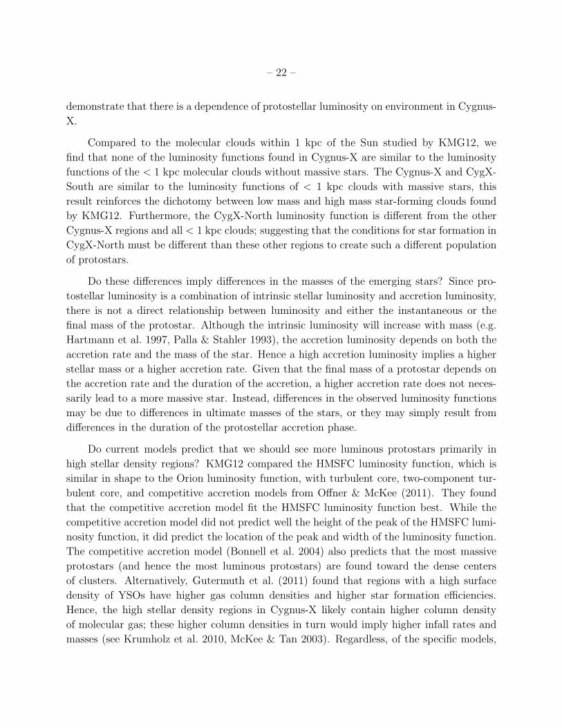
Fig. 7.— Log(<RMEDSQ>Dc) vs. log(Lbol/L⊙) for protostar candidates in the full Cygnus-

X sample (left), CygX-North sample (middle), and CygX-South sample (right). All protostar

candidates projected on regions with AV > 3 are shown in black or green. The luminosity

cutoff Lcut and corresponding <RMEDSQ>Dc cutoff are shown by the red lines. The sources

below the <RMEDSQ>Dc decrease are the nebulosity filtered sample. The nebulosity filtered

sources which are above Lcut are used in our comparison of the luminosity functions; these

are colored in green.

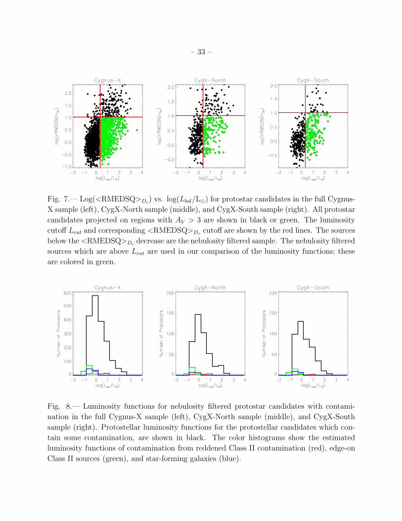
Fig. 8.— Luminosity functions for nebulosity filtered protostar candidates with contami-

nation in the full Cygnus-X sample (left), CygX-North sample (middle), and CygX-South

sample (right). Protostellar luminosity functions for the protostellar candidates which con-

tain some contamination, are shown in black. The color histograms show the estimated

luminosity functions of contamination from reddened Class II contamination (red), edge-on

Class II sources (green), and star-forming galaxies (blue).

– 34 –

Fig. 9.— Luminosity functions of nebulosity filtered protostars with estimated luminosities

of contamination from reddened disk sources, edge-on Class II sources, and background

galaxies removed for the Cygnus-X sample (left), CygX-North sample (middle), and CygX-

South sample (right). The vertical line shows the limiting Lbol (Lcut) found as the 90%

completeness limit in Section 2.3.1.

– 35 –

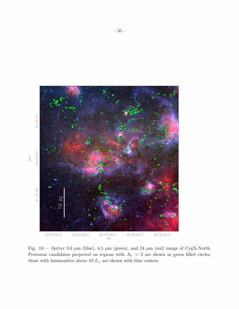
Fig. 10.— Spitzer 3.6 µm (blue), 4.5 µm (green), and 24 µm (red) image of CygX-North.

Protostar candidates projected on regions with AV > 3 are shown as green filled circles;

those with luminosities above 10 L⊙ are shown with blue centers.

– 36 –

Fig. 11.— Spitzer 3.6 µm (blue), 4.5 µm (green), and 24 µm (red) image of CygX-South.

Protostar candidates projected on regions with AV > 3 are shown as green filled circles;

those with luminosities above 10 L⊙ are shown with blue centers.

– 37 –

Fig. 12.— Nearest neighbor distances (for 4th nearest-neighbor YSO) and calculated bolo-

metric luminosity for the nebulosity filtered protostar candidates (<RMEDSQ>Dc< 10.41)

in the entire Cygnus-X sample (left), CygX-North sample (middle), and CygX-South sample

(right). The median protostar nn4 distance Dc is shown as a vertical red line, separating the

sample into high and low stellar density populations.

Fig. 13.— <RMEDSQ>Dc vs. nn4 distance for the entire Cygnus-X protostar candidate

sample (left), CygX-North protostar candidate sample (middle), and CygX-South protostar

candidate sample (right). The horizontal bar indicates the location of our RMEDSQ cut

above which we reject sources due to nebulosity discussed in Section 2.3.1. The vertical

bar shows Dc, the division between high and low stellar density populations. The protostar

candidates with luminosity greater than 10 L⊙ are shown in green. We find the sources with

highest <RMEDSQ>Dc, regardless of luminosity, in regions of higher stellar density.

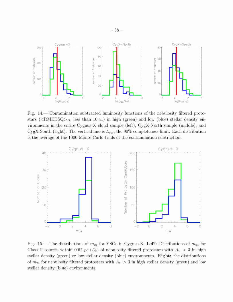
– 38 –

Fig. 14.— Contamination subtracted luminosity functions of the nebulosity filtered proto-

stars (<RMEDSQ>Dc less than 10.41) in high (green) and low (blue) stellar density en-

vironments in the entire Cygnus-X cloud sample (left), CygX-North sample (middle), and

CygX-South (right). The vertical line is Lcut, the 90% completeness limit. Each distribution

is the average of the 1000 Monte Carlo trials of the contamination subtraction.

Fig. 15.— The distributions of m24 for YSOs in Cygnus-X. Left: Distributions of m24 for

Class II sources within 0.62 pc (Dc) of nebulosity filtered protostars with AV > 3 in high

stellar density (green) or low stellar density (blue) environments. Right: the distributions

of m24 for nebulosity filtered protostars with AV > 3 in high stellar density (green) and low

stellar density (blue) environments.

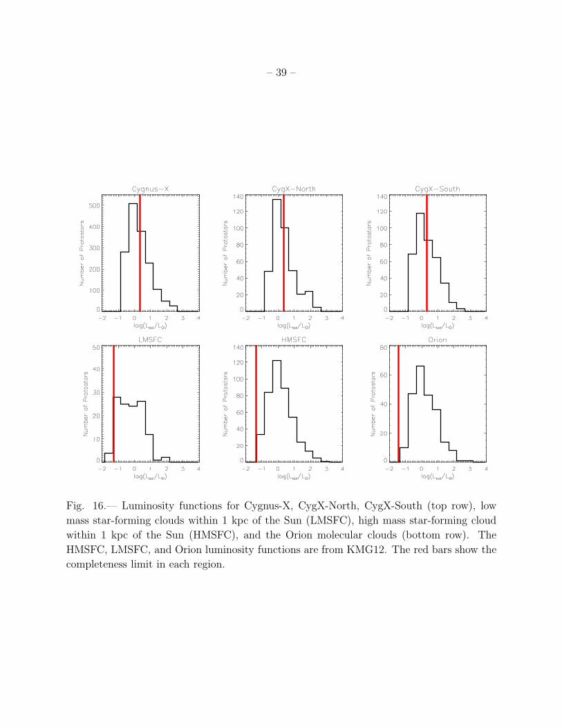
– 39 –

Fig. 16.— Luminosity functions for Cygnus-X, CygX-North, CygX-South (top row), low

mass star-forming clouds within 1 kpc of the Sun (LMSFC), high mass star-forming cloud

within 1 kpc of the Sun (HMSFC), and the Orion molecular clouds (bottom row). The

HMSFC, LMSFC, and Orion luminosity functions are from KMG12. The red bars show the

completeness limit in each region.

– 40 –

REFERENCES

Allen, L. E., Calvet, N., D’Alessio, P., et al. 2004, ApJS, 154, 363

Beerer, I. M., Koenig, X. P., Hora, J. L., et al. 2010, ApJ, 720, 679

Bressert, E., Bastian, N., Gutermuth, R., et al. 2010, MNRAS, 409, L54

Bonnell, I. A., Vine, S. G., & Bate, M. R. 2004, MNRAS, 349, 735

Bonnell, I. A., Smith, R. J., Clark, P. C., & Bate, M. R. 2011, MNRAS, 410, 2339

Bontemps, S., Andre, P., Kaas, A. A., et al. 2001, A&A, 372, 173

Bontemps, S., Motte, F., Csengeri, T., & Schneider, N. 2010, A&A, 524, A18

Calvet, N., Hartmann, L., Kenyon, S. J., & Whitney, B. A. 1994, ApJ, 434, 330

Carpenter, J. M. 2000, AJ, 120, 3139

Chapman, N. L., & Mundy, L. G. 2009, ApJ, 699, 1866

Clark, P. C., Bonnell, I. A., & Klessen, R. S. 2008, MNRAS, 386, 3

Comeron, F., & Pasquali, A. 2012, A&A, 543, A101

Crapsi, A., van Dishoeck, E. F., Hogerheijde, M. R., Pontoppidan, K. M., & Dullemond,

C. P. 2008, A&A, 486, 245

Cutri, R. M., Skrutskie, M. F., van Dyk, S., et al. 2003, The IRSA 2MASS All-Sky Point

Source Catalog, NASA/IPAC Infrared Science Archive

Davis, C. J., Kumar, M. S. N., Sandell, G., et al. 2007, MNRAS, 374, 29

Deharveng, L., Schuller, F., Anderson, L. D., Zavagno, A., Wyrowski, F., Menten, K. M.,

Bronfman, L., Testi, L., Walmsley, C. M. & Wienen, M. 2010 A&A, 523, 6

Deharveng, L., Zavagno, A., Anderson, L. D., Motte, F., Abergel, A., Andre, P., Bontemps,

S., Leleu, G., Roussel, H. and Russeil, D. 2012 A&A, 546, 74.

Dickel, H. R., Wendker, H., & Bieritz, J. H. 1969, A&A, 1, 270

Enoch, M. L., Evans, N. J., II, Sargent, A. I., & Glenn, J. 2009, ApJ, 692, 973

Evans, N. J., II, Dunham, M. M., Jørgensen, J. K., et al. 2009, ApJS, 181, 321

– 41 –

Fazio, G. G., Hora, J. L., Allen, L. E., et al. 2004, ApJS, 154, 10

Fischer, W. J., Megeath, S. T., Ali, B., Tobin, J. J., Osorio, M., Allen, L. E., Kryukova,

E., Stanke, T., Stutz, A. M., Bergin, E., Calvet, N., di Francesco, J., Furlan, E.

Hartmann, L., Henning, T., Krause, O., Manoj, P., Maret, S., Muzerolle, J., Myers,

P., Neufeld, D., Pontoppidan, K., Poteet, C. A., Watson, D. M. Wilson, T. 2010

A&A518, 122

Greene, T. P., Wilking, B. A., Andre, P., Young, E. T., & Lada, C. J. 1994, ApJ, 434, 614

Gutermuth, R. A., Pipher, J. L., Megeath, S. T., et al. 2011, ApJ, 739, 84

Gutermuth, R. A., Megeath, S. T., Myers, P. C., et al. 2009, ApJS, 184, 18

Gutermuth, R. A., et al. 2008, ApJ, 674, 336

Hanson, M. M. 2003, ApJ, 597, 957

Hartmann, L., Cassen, P., & Kenyon, S. J. 1997, ApJ, 475, 770

Harvey, P., Merın, B., Huard, T. L., et al. 2007, ApJ, 663, 1149

Hennemann, M., Motte, F., Schneider, N., et al. 2012, A&A, 543, L3

Hsu, W.-H., Hartmann, L., Allen, L., et al. 2012, ApJ, 752, 59

Hsu, W.-H., Hartmann, L., Allen, L., et al. 2012, ApJ, 764, 114

Knodlseder, J. 2000, A&A, 360, 539

Krumholz, M. R., Cunningham, A. J., Klein, R. I., & McKee, C. F. 2010, ApJ, 713, 1120

Kryukova, E., Megeath, S. T., Gutermuth, R. A., et al. 2012, AJ, 144, 31

Lada, C. J., & Wilking, B. A. 1984, ApJ, 287, 610

Landecker, T. L. 1984, AJ, 89, 95

Lonsdale, C. J., Smith, H. E., Rowan-Robinson, M., et al. 2003, PASP, 115, 897

Lucas, P. W., Hoare, M. G., Longmore, A., et al. 2008, MNRAS, 391, 136

McClure, M. K., Furlan, E., Manoj, P., et al. 2010, ApJS, 188, 75

McKee, C. F., & Tan, J. C. 2003, ApJ, 585, 850

– 42 –

Massey, P., & Thompson, A. B. 1991, AJ, 101, 1408

Megeath, S. T. & Wilson, T. L. 1997, AJ114, 1106

Megeath, S. T., Allen, L. E., Gutermuth, R. A., et al. 2004, ApJS, 154, 367

Megeath, S. T., Allgaier, E., Young, E., et al. 2009, AJ, 137, 4072

Megeath, S. T., Gutermuth, R., Muzerolle, J., Kryukova, E., Flaherty, K., Hora, J., Allen,

L. E., Hartmann, L., Myers, P. C., Pipher, J. L., Stauffer, J., Young, E. T., Fazio,

G. G., et al. 2012, AJ, 144, 192

Motte, F., Bontemps, S., Schilke, P., et al. 2007, A&A, 476, 1243

Muzerolle, J., Megeath, S. T., Gutermuth, R. A., et al. 2004, ApJS, 154, 379

Offner, S. S. R., & McKee, C. F. 2011, ApJ, 736, 53

Palla, F., & Stahler, S. W. 1993, ApJ, 418, 414

Polychroni, D., Schisano, E., Elia, D., Roy, A., Molinari, S., Martin, P., Andre, P., Tur-

rini, D., Rygl, K. L. J., Benedettini, M., Busquet, G., di Giorgio, A. M., Pestalozzi,

M., Pezzuto, S., Arzoumanian, D., Bontemps, S., Di Francesco, J., Hennemann, M.,

Hill, T., Konyves, V., Menshchikov, A., Motte, F., Nguyen-Luong, Q., Peretto, N.,

Schneider, N. and White, G. 2013arXiv1309.2332P

Rieke, G. H., Young, E. T., Engelbracht, C. W., et al. 2004, ApJS, 154, 25

Reipurth, B., & Schneider, N. 2008, Handbook of Star Forming Regions, Volume I, 36

Robitaille, T. P., Whitney, B. A., Indebetouw, R., Wood, K., & Denzmore, P. 2006, ApJS,

167, 256

Rygl, K. L. J., Brunthaler, A., Sanna, A., et al. 2012, A&A, 539, A79

Schneider, N., Gusten, R., Tremblin, P., et al. 2012, A&A, 542, L18

Schneider, N., Bontemps, S., Simon, R., et al. 2011, A&A, 529, A1

Schneider, N., Csengeri, T., Bontemps, S., Motte, F. Simon, R., Hennebelle P., Federrath,

C. & Klessen, R., A&A, 520, A49

Schneider, N., Simon, R., Bontemps, S., Comeron, F., & Motte, F. 2007, A&A, 474, 873

Schneider, N., Bontemps, S., Simon, R., et al. 2006, A&A, 458, 855

– 43 –

Skrutskie, M. F., Cutri, R. M., Stiening, R., et al. 2006, AJ, 131, 1163

, Stutz, A. M., Tobin, J. J., Stanke, T., Megeath, S. T., Fischer, W. J., Robitaille, T.,

Henning, T. Ali, B., di Francesco, J., Furlan, E., Hartmann, L., Osorio, M., Wilson,

T. L., Allen, L., Krause, O. and Manoj, P. 2013 ApJ, 767, 36.

Whitney, B. A., Indebetouw, R., Bjorkman, J. E., & Wood, K. 2004, ApJ, 617, 1177

Wilson, B. A., Dame, T. M., Masheder, M. R. W., & Thaddeus, P. 2005, A&A, 430, 523

Winston, E., Megeath, S. T., Wolk, S. J., et al. 2007, ApJ, 669, 493

Wright, N. J., Bouy, H., Drake, J. J., et al. 2012, arXiv:1208.0211

Wright, N. J., Drake, J. J., Drew, J. E., et al. 2012, ApJ, 746, L21

Wright, N. J., Drake, J. J., Drew, J. E., & Vink, J. S. 2010, ApJ, 713, 871

Zapata, L. A., Loinard, L., Su, Y.-N., et al. 2012, ApJ, 744, 86

This preprint was prepared with the AAS LATEX macros v5.2.