The Demand for Food Away from Home: Full-Service or Fast Food?

Abstract

Consumer spending at full-service and fast food restaurants will continue to grow over theremainder of this decade and the next. However, the larger increase is predicted to occur atfull-service restaurants. Simulations assuming modest growth in household income plusexpected demographic developments show that per capita spending could rise by 18 percentat full-service restaurants and by 6 percent for fast food between 2000 and 2020. Theassumed increase in income alone causes such spending to rise by almost 15 percent and 7percent at full-service and fast food restaurants, respectively. The increasing proportion ofhouseholds containing a single person or multiple adults without live-at-home children willcause per person spending to rise by another 1 to 2 percent in each of these segments.However, the aging of the population will decrease spending on fast food by about 2 per-cent per capita.

Keywords: full-service restaurants, fast food restaurants, food spending, householdincome.

Acknowledgments

The authors thank Mark Denbaly and Nicole Ballenger for their assistance in preparingthis report. For review comments on earlier drafts, we also thank Oral Capps, Jr., JohnPark, Chung Huang, Wen Chern, and Geoffrey Paulin. Thanks too to Dale Simms forediting and production. Any remaining errors and omissions are solely the the responsi-bility of the authors.

United StatesDepartmentof Agriculture

www.ers.usda.gov

Electronic Report from the Economic Research Service

January 2004

AgriculturalEconomicReport No. 829

The Demand for Food Away From HomeFull-Service or Fast Food?

Hayden Stewart, Noel Blisard,Sanjib Bhuyan, and Rodolfo M. Nayga, Jr.

Contents

Summary . . . . . . . . . . . . . . . . . . . . . . . . . . . . . . . . . . . . . . . . . . . . . . . . . . . . . . . . . . . . . . . . . . . . .iii

Introduction . . . . . . . . . . . . . . . . . . . . . . . . . . . . . . . . . . . . . . . . . . . . . . . . . . . . . . . . . . . . . . . . . . .1

Determinants of Consumer Demand . . . . . . . . . . . . . . . . . . . . . . . . . . . . . . . . . . . . . . . . . . . . . . .3

Effect of Household Characteristics on Demand . . . . . . . . . . . . . . . . . . . . . . . . . . . . . . . . . . . . .4

Statistical Model of Away-From-Home Expenditures . . . . . . . . . . . . . . . . . . . . . . . . . . . . . . . . .6

Simulating Future Away-From-Home Expenditures . . . . . . . . . . . . . . . . . . . . . . . . . . . . . . . . . 11

Implications for Market Composition . . . . . . . . . . . . . . . . . . . . . . . . . . . . . . . . . . . . . . . . . . . . .15

References . . . . . . . . . . . . . . . . . . . . . . . . . . . . . . . . . . . . . . . . . . . . . . . . . . . . . . . . . . . . . . . . . . . .16

Appendix . . . . . . . . . . . . . . . . . . . . . . . . . . . . . . . . . . . . . . . . . . . . . . . . . . . . . . . . . . . . . . . . . . . . .18

ii ● Demand for Food Away From Home / AER-829 Economic Research Service/USDA

Summary

Consumer spending at full-service and fast food restaurants will continue to grow over theremainder of this decade and the next. However, the larger increase will likely occur at full-service restaurants. Simulations assuming modest growth in household income plusexpected demographic developments show that per capita spending could rise by 18 percentat full-service restaurants and by 6 percent for fast food between 2000 and 2020. Theassumed increase in income alone causes such spending to rise by almost 15 percent and 7percent at full-service and fast food restaurants, respectively. The increasing proportion ofhouseholds containing a single person or multiple adults without live-at-home children willcause per person spending to rise by another 1 to 2 percent in each of these segments.However, the aging of the population will decrease per person spending on fast food byabout 2 percent per capita.

Fast food restaurants had been increasing their share of the growing away-from-home mar-ket until the middle of the 1990s. Sales at fast food restaurants briefly surpassed those atfull-service restaurants around the same time. However, the fast food share of the away-from-home market has been relatively steady since then. In 2002, full-service restaurantsagain accounted for a slightly larger share of total sales.

A household's demand for food away from home depends on its income as well as on itsdemographics. A 10-percent increase in a typical household's per capita income wouldcause it to spend 6.4 percent and 3.2 percent more per capita at full-service and fast foodrestaurants, respectively. Away-from-home expenditures are typically higher for single-per-son households and households containing multiple adults without live-at-home children.For instance, a single person spends almost $3 more per person each week at each type ofestablishment than an otherwise identical person who is married and has live-at-home chil-dren.

Current and future changes in the away-from-home market could reflect changes in the dietand health of American consumers. Any shift in market share between fast food and full-service restaurants may reflect important changes in what people are eating away fromhome, because fast food tends to have different quantities of fat and calories than meals pre-pared at full-service restaurants.

This study also represents a necessary first step in understanding how and why the structureof the foodservice industry is changing. As the demand for meals and snacks at full-servicerestaurants increases relative to the demand for fast food, restaurant companies will bemotivated to adjust what menu items and services they offer. To be sure, such adjustmentsmight also alter any projected changes in market share between full-service and fast foodestablishments.

Economic Research Service/USDA Demand for Food Away From Home / AER-829 ● iii

Introduction

Americans now spend nearly half of their food dollarson meals and snacks at foodservice facilities, such asrestaurants, hotels, and schools. Total away-from-home expenditures, defined to include all food dis-pensed for immediate consumption outside of theconsumer's home, amounted to $415 billion in 2002.1

That is about 58 percent greater than annual away-from-home expenditures in 1992 which totaled $263billion. Even after accounting for inflation and busi-ness cycles (fig. 1), expenditures still increased by 23percent between 1992 and 2002. We anticipate thathouseholds will continue to increase their spending onfoodservice meals and snacks at an annual rate ofabout 1.2 percent in real (inflation-adjusted) terms(Blisard et al., 2003).2 Rising household incomes anddemographic developments, such as smaller householdsizes, will account for this. However, it is not clearwhat types of foodservice facilities will be sellingthese meals and snacks.

A diverse array of foodservice firms—full-servicerestaurants, fast food establishments, hotels, retailstores, recreation places, bars, and operators of vend-ing machines—compete for the consumer's away-from-home dollar. However, full-service and fast foodrestaurants have captured the bulk of the market, with39.9 percent and 37.9 percent of total sales in 2002(fig. 2).3 Full-service restaurants, defined as establish-ments with waitstaff, tend to offer more varied menusand dining amenities. Fast food establishments tend toemphasize convenience (table 1).

The composition of the away-from-home market isdynamic. The full-service and fast food segments nowcommand a similar share of the market, but it isunclear which segment is poised to expand relative tothe other. Until the middle of the 1990s, sales of fastfood were increasing faster, and briefly surpassedthose at full-service restaurants. This upsurge wasbuoyed by the strategic location of new fast food out-lets. Convenience is a major sales point for fast foodoperators. If driving to an outlet takes longer thancooking at home, then fast food is not truly conven-ient.4 Thus, as fast food companies open more outletsper square mile in appropriate locations, consumershave to travel less for fast food, on average. In turn,these new store openings have stimulated the demandfor fast food (Jekanowski et al., 2001). The prolifera-tion of fast food restaurants can be seen in a trendknown as “channel-blurring,” whereby gas stations andretail stores, such as Wal-Mart and Target, are hostingfoodservice chains like Pizza Hut and Taco Bell.

Economic Research Service/USDA Demand for Food Away From Home / AER-829 ● 1

The Demand for Food Away From HomeFull-Service or Fast Food?

Hayden Stewart, Noel Blisard,Sanjib Bhuyan, and Rodolfo M. Nayga, Jr.*

* Sanjib Bhuyan is a member of the faculty at the Department ofAgricultural, Food, and Resource Economics at RutgersUniversity. Rodolfo M. Nayga, Jr., is a member of the faculty atthe Department of Agricultural Economics at Texas A&MUniversity.

1 Figures reported in this study are supplied by the EconomicResearch Service (ERS) and do not include alcohol. However,estimates of total expenditures do include the value of food con-sumed away from home, even if not purchased, such as the valueof food distributed in some institutional facilities, as well as taxesand tips. See Manchester (1987) for a more detailed explanationof how ERS figures are calculated, including the distinctionbetween sales and expenditures. Other sources report similar esti-mates of the market's size even though these sources base theircalculations on very different formulas. The National RestaurantAssociation, for one, emphasizes the value of sales by restaurantcompanies. For 2002, it estimated the value of sales at $407.8 bil-lion.2 Industry studies have also projected the continued growth of themarket including analyses by the National Restaurant Association(Restaurant Industry 2010: The Road Ahead) and a consultingfirm (Foodservice 2010).

3 The National Restaurant Association estimates that, in 2002,sales by full-service restaurants totaled $146 billion and sales byfast food restaurants amounted to $116 billion (Restaurant IndustryForecast 2003). 4 Making a meal convenient includes building outlets near whereconsumers live, work, and shop. Convenience also means speedyservice. For example, when it comes to drive-thru service, itappears that a goal among fast food chains is to serve customers inunder 3 minutes. In 2002, the average service time—from when acar reaches the speaker to the car's driver receiving his or herfood—at 25 major chains was about 187 seconds (Tutor, 2003).

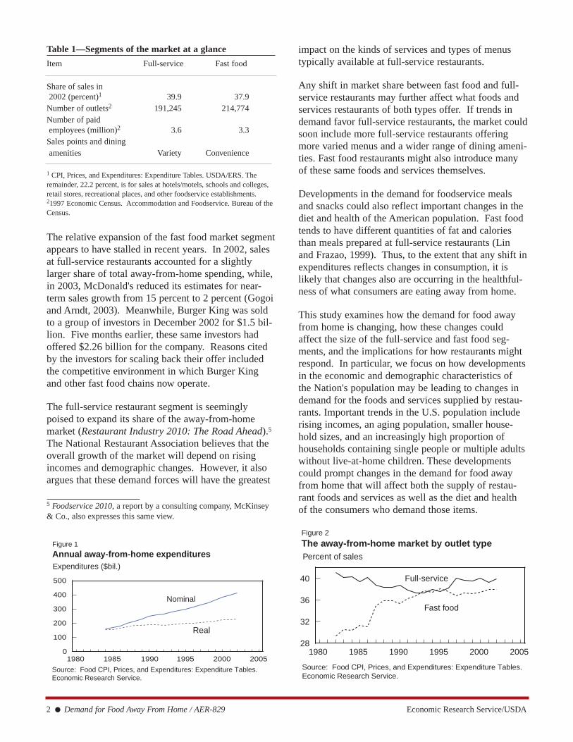
The relative expansion of the fast food market segmentappears to have stalled in recent years. In 2002, salesat full-service restaurants accounted for a slightlylarger share of total away-from-home spending, while,in 2003, McDonald's reduced its estimates for near-term sales growth from 15 percent to 2 percent (Gogoiand Arndt, 2003). Meanwhile, Burger King was soldto a group of investors in December 2002 for $1.5 bil-lion. Five months earlier, these same investors hadoffered $2.26 billion for the company. Reasons citedby the investors for scaling back their offer includedthe competitive environment in which Burger Kingand other fast food chains now operate.

The full-service restaurant segment is seeminglypoised to expand its share of the away-from-homemarket (Restaurant Industry 2010: The Road Ahead).5

The National Restaurant Association believes that theoverall growth of the market will depend on risingincomes and demographic changes. However, it alsoargues that these demand forces will have the greatest

impact on the kinds of services and types of menustypically available at full-service restaurants.

Any shift in market share between fast food and full-service restaurants may further affect what foods andservices restaurants of both types offer. If trends indemand favor full-service restaurants, the market couldsoon include more full-service restaurants offeringmore varied menus and a wider range of dining ameni-ties. Fast food restaurants might also introduce manyof these same foods and services themselves.

Developments in the demand for foodservice mealsand snacks could also reflect important changes in thediet and health of the American population. Fast foodtends to have different quantities of fat and caloriesthan meals prepared at full-service restaurants (Linand Frazao, 1999). Thus, to the extent that any shift inexpenditures reflects changes in consumption, it islikely that changes also are occurring in the healthful-ness of what consumers are eating away from home.

This study examines how the demand for food awayfrom home is changing, how these changes couldaffect the size of the full-service and fast food seg-ments, and the implications for how restaurants mightrespond. In particular, we focus on how developmentsin the economic and demographic characteristics ofthe Nation's population may be leading to changes indemand for the foods and services supplied by restau-rants. Important trends in the U.S. population includerising incomes, an aging population, smaller house-hold sizes, and an increasingly high proportion ofhouseholds containing single people or multiple adultswithout live-at-home children. These developmentscould prompt changes in the demand for food awayfrom home that will affect both the supply of restau-rant foods and services as well as the diet and healthof the consumers who demand those items.

2 ● Demand for Food Away From Home / AER-829 Economic Research Service/USDA

Table 1—Segments of the market at a glance

Item Full-service Fast food

Share of sales in2002 (percent)1 39.9 37.9

Number of outlets2 191,245 214,774Number of paidemployees (million)2 3.6 3.3

Sales points and diningamenities Variety Convenience

1 CPI, Prices, and Expenditures: Expenditure Tables. USDA/ERS. Theremainder, 22.2 percent, is for sales at hotels/motels, schools and colleges,retail stores, recreational places, and other foodservice establishments.21997 Economic Census. Accommodation and Foodservice. Bureau of theCensus.

Figure 1

Annual away-from-home expendituresExpenditures ($bil.)

Real

Source: Food CPI, Prices, and Expenditures: Expenditure Tables.Economic Research Service.

1980 1985 1990 1995 2000 20050

100

200

300

400

500

Nominal

Figure 2

The away-from-home market by outlet typePercent of sales

Source: Food CPI, Prices, and Expenditures: Expenditure Tables.Economic Research Service.

1980 1985 1990 1995 2000 200528

32

36

40 Full-service

Fast food

5 Foodservice 2010, a report by a consulting company, McKinsey& Co., also expresses this same view.

Real

Determinants of Consumer Demand

The theory of household production, outlined byBecker (1965), extends classical demand theory toconsider how prices, income, demographics, and timeconstraints can all influence a household's purchasesof items like food. This economic model of householdbehavior holds that the costs of consumption caninclude prices as well as time spent eating food,preparing food, and cleaning up after a meal or snack.A household must therefore decide whether to spendtime on all aspects of the activity of eating a meal (i.e.,prepare food at home) or outsource some aspects likepreparation and cleaning up (i.e., purchase food awayfrom home). The optimal decision depends on manyfactors, including the household's finances, the oppor-tunity cost of its manager's time, and how well thehousehold manager can cook. In the context ofBecker's model, a household manager can be definedas the person primarily responsible for shopping,cooking, cleaning, and other household chores.

Empirical analyses have further shown how specificeconomic and demographic characteristics of a house-hold can influence its demand for food away fromhome by market segment. Four such studies usehousehold survey data from the 1970s and 1980s.McCracken and Brandt (1987) and Byrne et al. (1998)analyzed the relationship between some key householdcharacteristics and expenditures at each type of restau-rant. Nayga and Capps (1994) studied the relationshipbetween a household's characteristics and its frequencyof dining at each type of facility. Also, Hiemstra andKim (1995) analyzed the impact of household charac-teristics on expenditure by eating occasion and marketsegment.6 Characteristics found to be important inthese studies include the household's income, timeconstraints faced by the household manager, thehousehold manager's age, number of people in thehousehold, education level of the household manager,the household's region of residence, and the house-hold's race and ethnicity.

Households with higher incomes tend to spend moreon products and services, including leisure, variety,and dining amenities like waitstaff, ambience, andalcohol service. Food away from home is a form of

leisure where leisure is defined as time spent outsideof both the labor force and household production.Both fast food and full-service restaurants can provideleisure for a household manager who is freed fromcooking, cleaning, and shopping. Moreover, alongwith the additional leisure, households with moreincome may also buy more variety and other diningamenities. Thus, households with higher incomeshave been shown to have higher expenditures for bothfast food and full-service meals and snacks, but spend-ing at full-service restaurants is most responsive to anychanges in income (e.g., McCracken and Brandt,1987; Byrne et al., 1998).

Households also may demand more food away fromhome as their manager works longer hours outside thehome. In particular, fast food may come to represent aconvenient meal option, if such a restaurant is reason-ably accessible. Spending for fast food has beenshown to increase along with the number of hoursworked by a household manager in the labor force(e.g., Byrne et al., 1998). By contrast, dining at a full-service restaurant can take as long as preparing, eating,and cleaning up after a meal at home. Thus, there isneither a clear theoretical nor empirical relationshipbetween a household's demand for food at full-servicerestaurants and its time constraints.

The number of people living in a household also mayinfluence its demand for meals and snacks away fromhome. In particular, as a household adds more mem-bers, food prepared at home may become more eco-nomical. For example, it might take 20 minutes toprepare a meal for one person at home, but just 30minutes to prepare a meal for four people. Whencooking at home, the household with more memberscan also benefit by purchasing larger package sizeswith lower per unit costs. In total, single-personhouseholds will likely have the highest time and mon-etary costs per person for eating at home, while largerhouseholds will incur lower costs per capita.Empirical studies do find that larger households tendto spend less money per capita away from home (e.g.,McCracken and Brandt, 1987).

A household's demand for food away from home alsomay depend on the ages of its members. One reasonis that tastes may change as people age. For example,if the sensitivity of taste buds diminishes with age,older people may demand foods with bolder flavors(Friddle et al., 2001). Also, older and younger peoplemay have different opportunities to socialize, so if they


6 Eating occasion was defined to include, for example, breakfast,lunch, and dinner.

eat out for different reasons, they may logically go todifferent kinds of establishments. On balance, empiri-cal studies find that households with younger memberstend to spend more money on fast food, while house-holds with older people tend to spend more money onfull-service dining (Byrne et al., 1998).

The impact of aging on demand is complicated byuncertainty about whether generations will retain theirdistinctive eating habits as they age. For example, willan elderly person in 2020 have the same expenditurepatterns as an elderly person now with similar charac-teristics? Perhaps not. Younger generations know lessabout cooking than earlier generations did at the samepoint in their life (Foodservice 2010). However, evenif this argument is true, younger generations may stillevolve like older generations. Younger generationsmay compensate for their lack of skills by takingadvantage of the growing array of prepared foods andconvenience appliances. In fact, Blisard (2001) findsthat members of different generations tend to havesimilar behavior away from home at the same points intheir lives.

Does the structure of a household also influence itsdemand for meals and snacks away from home? Forinstance, a married couple with children is likely tohave different preferences and preparation capabilitiesthan a single-parent family, a single-person household,and multiple adults living together without children.Even after controlling for hours worked in the laborforce and income, members of each of these types ofhousehold may not share the same opportunities tosocialize or face the same time constraints. This is asubject area not taken up by previous research.

Effect of HouseholdCharacteristics on Demand

Our first step in this analysis is to identify the charac-teristics of a household that are potential determinantsof its demand for food away from home. In additionto characteristics identified in past studies, we includethe structure of a household, whether it is comprisedof a married couple with children, a single parent withchildren, a single person, or multiple adults withoutlive-at-home children. A data set must also be identi-fied to empirically examine the relationships betweenthe characteristics of a household and that household'sdemand for meals and snacks at both fast food andfull-service restaurants.

Changing Structure of Households

The increasing incidence of alternative types of house-hold in the U.S. has been much publicized (e.g.,Kinsey, 1990). In this study, we define a traditionalhousehold as a married couple with live-at-home chil-dren. Traditional households accounted for 30.2 per-cent of all households in 1980, but just 23.5 percent in2000 (Cromartie, 2002). Single-person households,single-parent families, and households of multipleadults without a live-at-home child are on the rise (seebox, “Changing Structure of American Households”).

Differences are likely to exist in the preferences andhousehold production capabilities of diverse types ofhouseholds. Members of single-person householdsmay be more likely to socialize and date than membersof a traditional family. But do these pursuits inflateone's expenditures at full-service or fast food establish-ments? For example, dating might lend itself to full-service restaurants promising a leisurely diningexperience, while fast food establishments with playfacilities may appeal more to families with children.

Single-parent households also may differ from tradi-tional households in that they are more likely to con-tend with limited social opportunities, financialinsecurity, and greater time constraints. These factorscould influence a single-parent household's demandfor convenience or other amenities associated withdining away from home.

A household with multiple adults and no child rearingresponsibilities could also be very different. Havingno children to raise could increase the household'sability to finance dining away from home, and expandits set of social opportunities. Greater financialresources and fewer time constraints might encouragethe household to spend more money at full-servicerestaurants in particular.

Data Used in the Analysis

To test hypotheses about how a household's demandfor food away from home is affected by its structureand other characteristics, we need a data set withinformation on households, their characteristics, andhow much they spend in each market segment. Theideal set of data for this study would include informa-tion on at least several thousand households, the char-acteristics of each household, and how much each



Changing Structure of American Households

The structure of the American household is chang-ing. The average age is higher, people are bettereducated, and there are fewer members per house-holds. More Americans are also living outside of atraditional family (a married couple with live-at-home children).

A household's structure can have significant impli-cations for how it buys and prepares food. Forexample, families with three or more children areconsidered a prime market for the basic food ingre-dients and volume discounts traditionally providedby grocery stores (Kinsey, 1990).

Demographic changes are behind the increasing fre-quency of nontraditional households. There aremore "empty nest" adults living together after theirchildren have grown up, as well as more unmarriedpeople who are perhaps waiting longer to get mar-ried or who have been widowed (Cromartie, 2002).

This report seeks to determine whether nontradi-tional households eat out more or less often thantheir traditional counterparts, and where they tendto spend their money. For example, as comparedwith a married couple engaged in child rearing, sin-gle people may have more social opportunities todine out at full-service restaurants.

2000

Single person (25.8%)

Single parent (9.2%)

Traditional Family (23.5%)

Multiple adults, no Children (41.5%)




Multiple adults, no children (46%)

2020 (Projected)




Multiple adults, no children (39.8%)

1980

Source: Derived from Cromartie, 2002, who provides projectionsfor traditional, single-person, and single-parent households. Healso provides a projection for married couples without children.However, these four categories are not all encompassing. Somehousehold types do not belong to any group, e.g., unmarried,cohabitating adults without children. Thus, in this study, wederived projections for households comprised of multiple adultswithout children by determining the percentage of households notbelonging to any one of the other three groups. It follows that thisfourth group includes all households with multiple adults and nochildren.

household spent in each market segment. Moreover, itwould follow this sample of households over 20 to 50years, and report on how each household's characteris-tics and expenditures have changed. By witnessinghow each household's food spending changed with itscharacteristics, we might project how spending islikely to further evolve as each current householdbecomes wealthier, older, or different in structure.Unfortunately, these data are not available. Still,employing some assumptions, we can adapt existingsources of data to undertake the same sort of analysis.

The Bureau of Labor Statistics (BLS) provides theonly public survey of household characteristics andhousehold expenditures.7 The BLS ConsumerExpenditure Survey (CES) is an annual representativesample of spending by American households.8 In thediary section of the survey, each household reports itsexpenditures on food away from home and othergoods for 2 weeks. These data can also be matchedwith information about each household, such as itsincome, number of members, region, and race.

The CES does not follow the same households overtime, and it does not classify household expendituresaway from home prior to 1998. The BLS surveys ahousehold for one 2-week period, and then drops thishousehold from its survey. Thus, each annual surveycontains a completely different set of households.Moreover, because the BLS did not break down away-from-home spending on fast food versus food at full-service restaurants prior to 1998, we can only use dataon household characteristics and their spending pat-terns for 1998, 1999, and 2000.9

An additional limitation of household surveys in gen-eral, including the CES, is that they do not include

expenditures by businesses or for people in institu-tions. It follows that the analysis in this study doesnot capture all of the away-from-home market. Inorder to determine how much of the market is capturedby the CES, we undertook a “back of the envelope”calculation. In 2000, among households completingthe survey, we find that per capita away-from-homespending averaged $19.21 each week, not includingalcohol. It follows that households in the UnitedStates spent about $1,000 per person per year. Thus,since the U.S. population equaled 281 million in 2000,it can be further estimated that spending by all house-holds was around $281 billion. We estimate that theCES captures about 75 percent of the total market,since the size of the away-from-home market wasapproximately $385 billion in 2000 (fig. 1).

Statistical Model of Away-From-Home Expenditures

The statistical model used in this report relates ahousehold's pattern of spending away from home to itseconomic and demographic characteristics, but not toprices. We recognize that prices are an importantdeterminant of demand. However, since the CES doesnot contain information on prices and our data werecollected over a short period of time, we assume thatthere was little variation in the price of fast food rela-tive to the price of food at full-service restaurants overthe period when the data were collected. In otherwords, households are assumed to have faced similarrelative prices.10 This assumption allows us to view ahousehold's expenditures on meals and snacks asvalue-weighted quantities. For example, a meal at afull-service restaurant may be more costly than a mealat a fast food restaurant. It is therefore possible that ahousehold eats fast food more often than full-servicemeals, but reports similar expenditures in both marketsegments. In this case, price differences serve to


7 The National Panel Diary Group (NPD) also undertakes such asurvey, Consumer Reports on Eating Share Trends (CREST).However, these data have not been available for use by outsideresearchers in recent years. 8 It includes only noninstitutional households. An institutionalhousehold would include people living in institutions, such as pris-ons or military facilities.9 We also removed households providing incomplete informationon key characteristics and/or reporting negative incomes from thesample. The CES designates households as "complete" or "incom-plete" income reporters, depending on their response to incomequestions. The distinction between complete and incompletereporters is based, in general, on whether or not the respondentprovided values for major sources of income, such as wages andsalaries, self-employment income, and Social Security income.However, even complete income reporters may not have provided afull accounting of all income from all sources. It is also possible

for complete reporters to report negative incomes due to self-employment or other income losses. In this study, incompleteincome reporters and complete reporters with negative incomes areexcluded. In each year, the final sample includes about 5,000households. 10 Our data were collected over 3 years. We allow prices to varyfrom year to year. We also allow prices to depend upon the seasonof the year when the survey was administered as well as upon theregion of the country in which the household resides. Householdsare assumed to face similar prices otherwise. Studies of the away-from-home market commonly make this same assumption, includ-ing McCracken and Brandt (1987) and Byrne et al. (1998).

weight the value of purchases to the household. Infact, a similarity of expenditures in the two segmentswould suggest that the household receives similar lev-els of satisfaction from its total purchases of bothtypes of food away from home. Viewing prices asweights for aggregating purchases in this way is con-sistent with classical demand theory (Green, 1964).

The Statistical Model

The statistical model will provide more accurate esti-mates of the relationships between a household's char-acteristics and its spending away from home, if wesimultaneously estimate the equations for spending onfast food and spending at full-service restaurants. Forinstance, because of variation in how much householdmanagers enjoy (or dislike) cooking, some householdsmay eat out relatively infrequently (or frequently) atboth types of facility. If so, a correlation is said toexist between a household's spending at full-servicerestaurants and the same household's spending on fastfood. Including this correlation in the model willimprove its accuracy, which can be accomplishedusing existing procedures for simultaneously estimat-ing models with multiple equations.11

Obtaining accurate estimates of the relationshipbetween household characteristics and away-from-home expenditures requires a special statistical proce-dure to account for households that do not have anysuch expenditures. During the 2-week survey period,21 percent of households completing the CES spent nomoney on fast food, and 45 percent spent no money ata full-service restaurant. This lack of purchases isknown as zero-censoring, and raises some estimationproblems. If the data contain many zero-expenditureobservations, results based on usual methods of esti-mation could be biased.

Models that allow a researcher to estimate multipleequations simultaneously and to account for zero-cen-soring include those developed by Heien and Wessells(1990) and Shonkwiler and Yen (1999). Here, weapply the latter model because it appears to be themost accurate and is “state-of-the-art.”12 A brief

description of this model follows, and a more detaileddescription is supplied in the appendix.

The Shonkwiler and Yen method proceeds in two stepsto correct for the problem of zero-censoring. In ourstudy, the first step analyzes whether each householdcompleting the CES had non-zero expenditures in eachmarket segment. In particular, the probability that ahousehold spends some money on fast food is esti-mated as a function of the household's income, timeconstraints, and demographic characteristics. Thesame equation is also estimated for each household'sdecision about whether to spend some money at full-service restaurants. These results are then used in thesecond step. At this point, we derive equations relat-ing a household's income and demographic character-istics to its expenditures in both market segments.These equations contain an adjustment to correct forthe fact that many households spent nothing, which isbased on the results of estimating the aforementionedprobabilities in the first step. The adjusted equationsfor spending at fast food and at full-service restaurantscan then be estimated using ordinary techniques forthe simultaneous estimation of multiple equations.

Definition of Variables

Data in the CES must be prepared for use in the statis-tical model before the analysis can be conducted. Inparticular, variables must be calculated from the rawdata in the CES. We specify and create several vari-ables, such as measures of household expenditures,household income, hours worked by household man-agers, household structure, the age of a householdmanager, and the number of people living in a house-hold (table 2).

To calculate the values of per capita expenditures atfast food and full-service restaurants, we divided ahousehold's weekly expenditures at each type of facil-ity by the number of members in the household.Inflation-adjusted spending was then determined bydividing expenditures by the Consumer Price Index(CPI)13 for all items.


11 This procedure is known as a seemingly unrelated regression.12 The method of Heien and Wessells (1990) has been widelyapplied over the past decade, including by Byrne et al. (1998).However, Shonkwiler and Yen (1999) have found a shortcoming ofthis model and present an alternative specification. Furthermore,

they use Monte Carlo techniques to demonstrate that their pro-posed specification is statistically more accurate. The method ofShonkwiler and Yen (1999) has been recently applied in severalstudies (e.g., Su and Yen, 2000 ; Yen et al., 2002).13 Fourth quarter of 2000 = 100.

Since income is a key variable that explains spending,we calculated this variable from data in the CES aswell. To do so, we divided a household's total incomeby the number of household members to obtain percapita income. Per capita income was then madeweekly (divided by 52) and stated in real terms(divided by the CPI).

Data in the CES were also used to calculate hoursworked each week outside of the home by the house-hold manager. However, the CES does not identify thehousehold manager—the person primarily responsiblefor household chores. Yen (1993), who also used theCES, circumvented this issue by studying the impactof hours worked by married women. However, thisstudy takes a slightly different approach. Each house-hold's manager is defined as the survey respondent ifthe person was single. For married respondents, thehousehold manager is assumed to be the spouse whoworks the fewest hours outside the home.14

Three binary variables were also created to capturehousehold structure. Each variable corresponds to oneof the three nontraditional types of household identi-fied in this report. These variables equal “one” if thehousehold belongs to a certain type, and “zero” other-wise. For example, one variable identifies whether ahousehold includes only a single person. It equalsone for the 28 percent of households in our samplewho are single, and zero for the other 72 percent. Allhouseholds were classified as belonging to either one


14 This approach is straightforward for households with either onlyone adult or a married couple. However, it may be less clear whenapplied to households with multiple unmarried adults, e.g., same-sex couples. In such a case, the household manager is always thesurvey respondent. There are two reasons for this defaultapproach. First, the CES does not include information on adults ina household who are not married to the survey respondent.Second, it is arguable that the action of responding to the CES isitself a domestic chore. If so, it is further likely that the personwho maintains the diary section of the CES is the primary house-hold manager.

Table 2—Variables measuring expenditures and household characteristics, calculated from CES

Variable Mean Definition

Expenditures:

Full-service restaurant $8.43 Per capita, average weekly spending at full-service restaurantsFast food $8.15 Per capita, average weekly spending on fast food

Household characteristics:

Income $422.00 Household's per capita, average weekly, real, before-tax income Hours worked

by manager 24.2 Hours spent in the labor force by the household managerAge of manager 47.55 Age of the household managerCollege-educated manager 0.25 Indicator variable of whether household manager has a college educationSize of household 2.56 Number of members reported to be living in the household

Race:Asian 0.047 Indicator variable of whether respondent or spouse identified themselves as AsianBlack 0.09 Indicator variable of whether respondent or spouse identified themselves as BlackHispanic 0.11 Indicator variable of whether respondent or spouse identified themselves as Hispanic

Household type:Traditional 0.27 Indicator variable of whether respondent is married with live-at-home childrenSingle 0.28 Indicator variable of whether respondent lives aloneMultiple adults

without children 0.35 Indicator variable of whether respondent lives with at least one other adult but no childrenSingle parent 0.10 Indicator variable of whether respondent is an unmarried adult with live-at-home children

of the three types of nontraditional household or asbeing a traditional household.15

Other household characteristics in our model includethe age of the household manager; number of peopleliving in the household; whether the household man-ager had completed college or attained a higher levelof education; household region; year the survey wascompleted; season in which the survey was completed;and whether a member of the household describedhimself or herself as belonging to a minority groupincluding Black, Asian, or Hispanic.

Results of Model Estimation

The results of our statistical analysis agree with botheconomic theory and past studies. Household struc-ture, a variable not considered in past studies, also isfound to have a statistically significant impact on howmuch a household spends in each segment of the mar-ket. Estimated relationships are evaluated at the sam-ple means shown in table 2. The results describe howan average household could be expected to adjust itsexpenditures in response to a change in a variable,such as its income or household type (table 3). Otherstatistical results are supplied in the appendix.

Spending in both market segments responds positivelyto an increase in per capita income. However, a 10-percent increase in per capita income would cause atypical household to augment its per capita expendi-tures on fast food by about 3.2 percent, versus 6.4 per-cent for full-service restaurants. Like past studies,including Byrne et al. (1998) and McCracken andBrandt (1987), our analysis suggests that householdswith more income buy more leisure as well as more ofother dining amenities.

Time spent by the household manager in the laborforce also has significant implications for how much a

household spends away from home. Spending for fastfood is especially sensitive. A typical householdincreases its per capita spending on fast food by about1.4 percent following a 10-percent increase in thenumber of hours worked outside the home by its man-ager. By contrast, this same household would increaseits per person spending at full-service restaurants byonly about 0.5 percent. The link between time con-straints and spending for fast food—but not for full-service restaurants—has been established.

The impact of aging also varies by market segment.Households with older managers dine at fast foodestablishments less frequently and, as a consequence,spend less money. An increase of 10 percent in theage of a household manager reduces the same house-hold's per capita expenditures on fast food by about 6percent. However, the same increase in age does notnegatively affect spending at full-service restaurants(table 3). As other studies have found, people's prefer-ences for food and services may tend to favor full-service restaurants as they age.

Larger households spend less money per capita in bothmarket segments. This finding supports prior researcharguing that economies exist in purchasing and preparingmeals at home. A typical household can be expected toreduce such spending in both market segments about 2


Table 3—Relationship between household characteris-tics and expected expenditures

Characteristic Full-service Fast food

Change in expenditures due to a 10-percentincrease in the variable:

PercentIncome +6.4 +3.2 Hours worked by manager +0.53 +1.44Size of household -2.25 -1.74Age of manager +1.05 -5.99

Absolute change in expenditure due to householdtaking on the characteristic:

DollarsCollege-educated manager +2.15 +0.24 Single-person household +2.92 +2.68 Single-parent family -0.83 -0.83 Multiple adultswithout children +1.98 +0.89

Asian household +0.81 +0.39 Black household -2.87 +0.01Hispanic household -0.93 +0.14

15 For this reason, we did not include a variable to account forwhether a household was traditional. Since each household in thedata is classified as belonging to one type and only one type, aproper statistical analysis requires that we omit one category ofhousehold from the analysis. This omission creates the orthogonalrelationship among predictor variables that is required for estimat-ing a covariance matrix and conducting hypothesis tests. The con-sequence is that the identified relationships between the threevariables in the model and expenditures must be interpreted as ameasure of the difference in per capita weekly spending by thesehouseholds and traditional households.

percent following a 10-percent increase in the number ofpeople living in the household (table 3).

Household structure also is important. However,because of the way variables capturing this structureare defined, we must be careful to interpret our results.The most appropriate interpretation of variables cap-turing household structure is to consider how a nontra-ditional household with otherwise typicalcharacteristics would likely adjust its spending awayfrom home if it became a traditional household. Forexample, as compared with a traditional household,higher per capita expenditures are typical of single-person and childless households. Indeed, a single per-son spends almost $3 more per person at each type ofestablishment. Thus, a single person could beexpected to reduce his or her per capita spending awayfrom home by $3 (for both fast food and full-servicefood) if he or she married and had a child.

Single parents and their children are the only type ofhousehold tending to spend less per capita than tradi-tional households. Single parents spend about 83cents less per person at each type of establishmentthan do their married counterparts. It follows that amarried person with children and otherwise typicalcharacteristics can be expected to reduce spending onfast food by 83 cents per person per week should he orshe divorce or become widowed.

Other variables, like race and education, are also sig-nificant determinants of how much a household spendsaway from home. For instance, between 1998 and2000, when all other variables are set at their meanvalue, a Black household still spent $2.87 less per per-son at full-service restaurants than did other house-holds (table 3). This finding is consistent with paststudies, and may reflect differences in tastes, or possi-bly more limited access to foodservice establishments.

Simulating Future Away-From-Home Expenditures

Future changes in demand can be simulated by incor-porating into our statistical model expectations abouthow key variables may change. These projectedchanges are based on modest growth in income, nochange in hours worked by household managers, andthe likely evolution of demographic variables, such asage of household managers, between 2000 and 2020.This same procedure has been used by Blaylock and

Smallwood (1986), Blisard and Blaylock (1993), andBlisard et al. (2003).

One way to interpret our simulation is as a snapshot ofhow people would have behaved in 2000, if the pro-jected changes in the population for 2020 were alreadyin place in 2000. For instance, we might ask howspending on fast food would have been different in2000 if household types assumed the same proportionsas we expect in 2020. This interpretation is the bestone because of a number of assumptions we have tomake. First, we assume there will be no change in theprice of fast food relative to the price of food at full-service restaurants. If such a change were to occur, itcould cause households to spend more or less than thesimulated amount. Second, we assume that householdcharacteristics will continue to influence consumerbehavior in the same way. For example, as a con-sumer moves from one demographic group to another,his or her preferences will take on the characteristicsof the new group. Thus, an elderly person in 2020 isassumed to have the same expenditure patterns as anelderly person in 2000 with similar characteristics(some evidence to justify this latter assumption is pro-vided by Blisard (2001) for the case of spending awayfrom home). Third, our simulation holds constant fac-tors like the number and location of restaurants as wellas the mix of food and services supplied by restau-rants. For instance, it is assumed that fast foodrestaurants will continue to supply the same types offood and the same dining amenities as they did in2000. We will later consider the significance of relax-ing this assumption, i.e., fast food restaurants offeringmore varied menus and heightened services.

Projected changes in the U.S. population include mod-est growth in household incomes. Real per capita dis-posable income increased by 1.2 percent per year onaverage between 1988 and 1998 (Saunders and Su,1999). Thus, we assume that per capita incomes willrise by 1 percent per year on an inflation-adjustedbasis between 2000 and 2020.16

No change is projected in the time constraints faced byhousehold managers, as we have found no compellingevidence to suggest that such changes will occur. Inrecent years, the growth in labor force participationamong adult women has slowed. The BLS reports thatparticipation was 51.6 percent in January 1980, 57.7percent in January 1990, and 60.3 percent in January


16 This same assumption was made in Blisard et al. (2003).

2000. It then fell back to 59.8 percent in December2002. We assume that, between 2000 and 2020, therewill be no further changes in labor force participation,nor in how much a typical household manager worksoutside of the home.

The future demographic characteristics of householdsare derived from Cromartie (2002).17 Population,household, and education projections used here arederived from reports by the U.S. Census Bureau. TheCensus Bureau population series includes projectionsby single year of age, sex, race, Hispanic origin, andnativity (foreign-born or native) out to the year 2100.By contrast, educational attainment projections by sexand race are available for the years 2003 and 2028, so

our numbers represent interpolations between thesetwo dates.

Projections derived from Cromartie (2002) are notintended as forecasts or predictions; rather, they repre-sent assumptions about future trends in population,household formation, schooling, and the economy atlarge. For instance, in the population series, projec-tions are based on assumptions about fertility, mortal-ity, and immigration. In fact, differing assumptionswere presented to provide three different projectionseries, representing high, middle, and low alternatives.This study uses projections based upon the middleseries. Despite uncertainty about the extent ofchanges, the finding in Cromartie (2002) is that theNation's future population will be older, better edu-cated, live in smaller households, be racially and ethni-cally more diverse, and live in more nontraditionaltypes of households (table 4).


Table 4—Current and projected future population characteristics, used in simulation

Characteristic 2000 2020Based on BLS reports:Income1 $422.10 $514.98 Hours worked by manager2 24.2 hours 24.2 hours

Based on Census projections:Size of household 2.5 members 2.4 membersAge of manager3 47.33 years 49.4 yearsCollege-educated manager 23.5% of households 26.4% of householdsSingle-person household 25.8% of households 28.6% of households Single-parent household 9.2% of households 8.7% of households Multiple adults, no children4 41.5% of households 46% of households Asian household 3.9% of households 5% of households Black household 12.3% of households 12.9% of households Hispanic household 12.6% of households 18% of households

1 Future income is calculated assuming a 1-percent rate of growth in per capita, real income. In particular, we used the formula for future value and continu-ous compounding, i.e., Income2020 = Income2000(1+0.01)202 No change is assumed in hours worked by household managers. Our assumption is based on the observation that measures of the working status of adultAmericans, such as the female labor force rate, have been relatively stable over the past 10 years.3 The age of a household manager is derived from projections in Cromartie (2002). It is the average age of all people older than 19 years. 4 Derived from Cromartie, 2002, who provides projections for traditional, single-person, and single-parent households. He also provides a projection for mar-ried couples without children. However, these four categories are not all encompassing. Some household types do not belong to any group, e.g., unmarried,cohabitating adults without children. Thus, in this study, we derived projections for households comprised of multiple adults by determining the percentage ofhouseholds who could not be classified as belonging to any one of the other three groups. It follows that this fourth group includes all households with multi-ple adults and no children.

17 Further information on how the projections in Cromartie (2002)are calculated can be found in Blisard et al. (2003).

Future Spending at Full-ServiceRestaurants

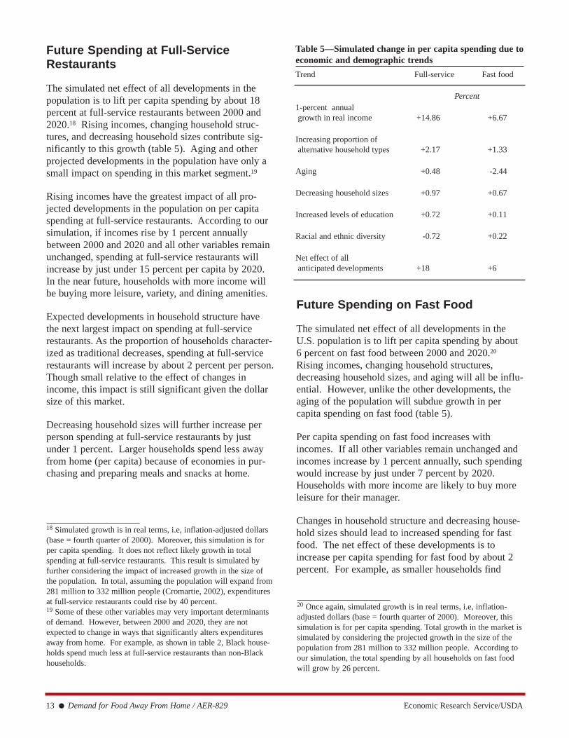
The simulated net effect of all developments in thepopulation is to lift per capita spending by about 18percent at full-service restaurants between 2000 and2020.18 Rising incomes, changing household struc-tures, and decreasing household sizes contribute sig-nificantly to this growth (table 5). Aging and otherprojected developments in the population have only asmall impact on spending in this market segment.19

Rising incomes have the greatest impact of all pro-jected developments in the population on per capitaspending at full-service restaurants. According to oursimulation, if incomes rise by 1 percent annuallybetween 2000 and 2020 and all other variables remainunchanged, spending at full-service restaurants willincrease by just under 15 percent per capita by 2020.In the near future, households with more income willbe buying more leisure, variety, and dining amenities.

Expected developments in household structure havethe next largest impact on spending at full-servicerestaurants. As the proportion of households character-ized as traditional decreases, spending at full-servicerestaurants will increase by about 2 percent per person.Though small relative to the effect of changes inincome, this impact is still significant given the dollarsize of this market.

Decreasing household sizes will further increase perperson spending at full-service restaurants by justunder 1 percent. Larger households spend less awayfrom home (per capita) because of economies in pur-chasing and preparing meals and snacks at home.

Future Spending on Fast Food

The simulated net effect of all developments in theU.S. population is to lift per capita spending by about6 percent on fast food between 2000 and 2020.20

Rising incomes, changing household structures,decreasing household sizes, and aging will all be influ-ential. However, unlike the other developments, theaging of the population will subdue growth in percapita spending on fast food (table 5).

Per capita spending on fast food increases withincomes. If all other variables remain unchanged andincomes increase by 1 percent annually, such spendingwould increase by just under 7 percent by 2020.Households with more income are likely to buy moreleisure for their manager.

Changes in household structure and decreasing house-hold sizes should lead to increased spending for fastfood. The net effect of these developments is toincrease per capita spending for fast food by about 2percent. For example, as smaller households find


Table 5—Simulated change in per capita spending due toeconomic and demographic trends

Trend Full-service Fast food

Percent1-percent annualgrowth in real income +14.86 +6.67

Increasing proportion ofalternative household types +2.17 +1.33

Aging +0.48 -2.44

Decreasing household sizes +0.97 +0.67

Increased levels of education +0.72 +0.11

Racial and ethnic diversity -0.72 +0.22

Net effect of allanticipated developments +18 +6

20 Once again, simulated growth is in real terms, i.e, inflation-adjusted dollars (base = fourth quarter of 2000). Moreover, thissimulation is for per capita spending. Total growth in the market issimulated by considering the projected growth in the size of thepopulation from 281 million to 332 million people. According toour simulation, the total spending by all households on fast foodwill grow by 26 percent.

18 Simulated growth is in real terms, i.e, inflation-adjusted dollars(base = fourth quarter of 2000). Moreover, this simulation is forper capita spending. It does not reflect likely growth in totalspending at full-service restaurants. This result is simulated byfurther considering the impact of increased growth in the size ofthe population. In total, assuming the population will expand from281 million to 332 million people (Cromartie, 2002), expendituresat full-service restaurants could rise by 40 percent. 19 Some of these other variables may very important determinantsof demand. However, between 2000 and 2020, they are notexpected to change in ways that significantly alters expendituresaway from home. For example, as shown in table 2, Black house-holds spend much less at full-service restaurants than non-Blackhouseholds.


The Changing Face of Fast Food

Many fast food restaurant companies are offering an increasingly wide range of goods and services. In fact, anew kind of restaurant concept is also emerging, fast-casual, which tries to combine the convenience of fastfood with the kinds of menus more typically found in a full-service restaurant. This changing face of fast foodcan be seen in the history of one of America's best-known restaurant chains, McDonald's.

McDonald's began as a fast food concept in 1948, when the McDonald brothers eliminated many of the menuitems and dining amenities previously available at their full-service restaurant. The remaining core menu hadsix products - hamburgers, cheeseburgers, fries, soft drinks, coffee, and shakes. The brothers also ceased toemploy waitstaff, and replaced their short-order cooks with workers who specialized at specific tasks likegrilling burgers. Says the company, "this limited menu concept triggered the 'fast food' concept, because focus-ing on just a few items that were prepared with standardized procedures made food service a model of effi-ciency" (McDonald's Corporation, media website).

The menu at McDonald's has gradually expanded to again include a wider variety of menu items. The firstaddition to McDonald's original menu was the Filet-O-Fish™ in 1963. A handful of other now well-knownproducts were then promoted over the next few decades including the Big Mac™ (1968), apple pie (1968),Egg McMuffin™ (1973), cookies (1974), and Chicken McNuggets™ (1983). However, according toConsortium Members, a group representing about 350 McDonald's franchisees, more recent new productintroductions have been the most "ambitious" in the company's history (Zuber, 2001).

Efforts to improve the atmosphere at McDonald's stores have accompanied efforts to expand menu items. Infact, the first McDonald's restaurant built to accommodate indoor seating was opened in 1962. However, themost noticeable efforts appear to be aimed at families with children. Ray Kroc, who became the company'sfranchising agent in 1954 and later purchased the McDonald's chain in 1961, is credited with focusing thecompany's marketing strategy on children through characters like Ronald McDonald. "A child who loves ourTV commercials," Kroc is quoted as saying, "and brings her grandparents to a McDonald's gives us two morecustomers" (Schlosser, 2001). Notable child-oriented goods and services include packaging meals for childrenwith toys, known as Happy Meals™ (1979), and installing play equipment in selected restaurants, known as aPlayland™ (1971).

Offering more goods and services has required McDonald's to rethink how its operates. In fact, in 1998, thecompany replaced its much-touted kitchens with the "Made for You" production system. According to thecompany, "Food is prepared to order for each customer. Somebody doesn't want pickles on a Big Mac orwants mustard on a grilled chicken sandwich? No problem…What's especially exciting is that this is far morethan just an operating system. It provides a platform for food innovation because it makes it easier to serve agreater variety of products" (McDonald's Corporation, 1998 Annual Report).

Many companies are promoting a newer concept, fast-casual, which strives to combine the food and atmos-phere of full-service restaurants with the convenience of fast food. Examples include Boston Market, Chili'sExpress, and Schlotzsky's Deli. As of 2003, the McDonald's Corporation continues to own Boston Market.

cooking at home relatively less economical than largerones, spending on fast food will grow.

The aging of the population will subdue any increasein spending due to changes in household structure andsize. Our simulation suggests that per person spendingon fast food may decrease by over 2 percent with theaging of the population. One possibility is that olderpeople derive less satisfaction from the foods and serv-ices traditionally offered at these establishments.

Implications for MarketComposition

Changes in demand are driving changes in the relativesizes of each segment of the away-from-home market.Rising incomes, the growing incidence of nontradi-tional households, and other developments in the U.S.population will allow for growth in both of the twolargest market segments. However, population trendsseem to favor increased spending at full-service restau-rants relative to fast food.

How might restaurant companies adjust their busi-nesses in response to the identified shift in demand?Our simulation has made some strict assumptionsabout prices and the behavior of consumers and firms.We now relax the assumption about firm behavior.

One plausible response by fast food companies wouldbe to introduce more of the foods and services tradi-tionally offered by full-service restaurants. In fact,among some companies, such a response appears to beunderway. For example, many Subway restaurantsaccept debit and credit cards, and McDonald's hasannounced the same—despite reservations about itseffect on the speed of its service. However, in testsusing high-speed connections, McDonald's found thatelectronic payments can now be processed in only 5seconds, versus 8 to 10 seconds for cash payments(CNNMoney, November 2002).

Many fast food restaurants are also expanding the vari-ety of their menus. A study by the NationalRestaurant Association estimated that more than 75percent of fast food restaurants introduced new menuitems in 2000, while 66 percent intended to add newfood items in 2001 (Operations Report 2001). AtMcDonald's restaurants, for example, Big Macs™ arenow sold alongside newer products like breakfastbagels, salads, fruit and yogurt parfaits, and soft-serve

ice cream with candy mix-ins. In 2003, the companywas further considering an increase in its scope ofhealthy menu items, including sliced fruits and vegeta-bles (see box, “The Changing Face of Fast Food”).

The response of fast food restaurant companies variesby firm, and the ability of many such restaurant com-panies to adapt may be limited. Marketing and logis-tics will likely prevent many fast food chains fromaggressively expanding their menus and/or scope ofservices. First, some chains appear to worry aboutconfusing their brand identity. Chick-fil-A, for one,added its first new category in 6 years in 2001, aportable salad line called “Cool Wraps.” The vicepresident of brand development conceded that “We arekind of a slow poke for development because webelieve in continuance of the menu” (Yee, 2001).21

Second, fast food chains may jeopardize the speed oftheir service in offering too many services or menuitems.

There is also the behavior of full-service restaurantcompanies to consider. These companies could bothopen more outlets and offer more variety/diningamenities at each establishment. In fact, in 2001, full-service restaurants were offering 31.6 percent moreitems on their menu than in 1997 (Yee, 2001). Theywere also increasing the scope of their services,including new options for takeout. In short, full-serv-ice restaurants may try to capture the growing demandfor varied menu items among consumers who alsoremain time-starved.

In conclusion, the relative growth of the fast food seg-ment appears to have stalled. Trends in demand nowfavor full-service dining. However, any changes inmarket share between the two segments will alsodepend on other factors, such as how firms in bothmarket segments change the mix of foods and servicessupplied to their customers. Future research is neededto better understand these later changes as well as theirimplications for industry structure and the health ofthe American population.22


21This survey did not include fine dining establishments (i.e.,restaurants with white tablecloths and a maitre'd).22ERS is currently undertaking a study of restaurants to determinehow they are adapting their menus and services. Evidence on thissubject admittedly is anecdotal at this point in time.

References

Becker, G. “A Theory of the Allocation of Time,”Economic Journal 75(1965): 493-517.

Blaylock, J., and D. Smallwood. U.S. Demand forFood: Household Expenditures, Demographics, andProjections, U.S. Department of Agriculture,Economic Research Service, TB-1713, 1986.

Blisard, N., and J. Blaylock. U.S. Demand for Food:Household Expenditures, Demographics, andProjections for 1990-2010, U.S. Department ofAgriculture, Economic Research Service, TB-1818,1993.

Blisard, N. Income and Food ExpendituresDecomposed by Cohort, Age, and Time Effects, U.S.Department of Agriculture, Economic ResearchService, TB-1896, 2001.

Blisard, N., J. Variyam, and J. Cromartie. FoodExpenditures by U.S. Households: Looking Aheadto 2020, U.S. Department of Agriculture, EconomicResearch Service, AER-821, 2003.

Byrne, P., O. Capps, Jr., and A. Saha. “Analysis ofFood-Away-from-Home Expenditure Patterns forU.S. Households, 1982-89,” American Journal ofAgricultural Economics 78(1996): 614-627.

Byrne, P., O. Capps Jr., and A. Saha. “Analysis ofQuick-serve, Mid-scale, and Up-scale Food Awayfrom Home Expenditures,” The International Foodand Agribusiness Management Review 1(1998): 51-72.

CNNMoney. “McDonald's to accept plastic,”11/26/2002. [Online]: www.cnn.com.

Consumer Expenditure Survey. Bureau of LaborStatistics. 1998, 1999, and 2000.

Cromartie, J. “Population Growth and DemographicChange, 1980-2020,” FoodReview 25,1 (2002): 10-12.

Food CPI, Prices, and Expenditures: ExpenditureTables. Economic Research Service. 04/30/03.[Online]: www.ers.usda.gov/briefing/CPIFoodAndExpenditures.

Foodservice 2010. McKinsey & Company, 2001.

Friddle, C., S. Mangaraj, and J. Kinsey. “The FoodService Industry: Trends and Changing Structure inthe New Millenium,” Working Paper #01-02, TheRetail Food Industry Center, University ofMinnesota, 2001.

Gogoi, P., and M. Arndt. “Hamburger Hell,” BusinessWeek, 3/3/2003, pp. 104-108.

Green, H. Aggregation in Economic Analysis,Princeton University Press, 1964.

Heien, D., and C. Wessells. “Demand SystemsEstimation with Microdata: A Censored RegressionApproach,” Journal of Business and EconomicStatistics 8(1990): 365-71.

Hiemstra, S., and W.G. Kim. “Factors AffectingExpenditures for Food Away From Home inCommercial Establishment by Type of Eating Placeand Meal Occasion,” Hospitality Research Journal19(1995): 15-31.

Jekanowski, M., J. Binkley, and J. Eales.“Convenience, Accessibility, and the Demand forFast Food,” Journal of Agricultural and ResourceEconomics 26(2001): 58-74.

Kinsey, J. “A graphic look at key economic figures.Diverse demographics drive the food industry,”Choices 5(1990): 22-23.

Lin, B., and E. Frazao. Away-From-Home FoodsIncreasingly Important to Quality of American Diet,U.S. Department of Agriculture, EconomicResearch Service, AIB-749, 1999.

Manchester, A. Developing an Integrated InformationSystem for the Food Sector, U.S. Department ofAgriculture, Economic Research Service, AER-575,1987.

McCracken, V., and J. Brandt. “HouseholdConsumption of Food Away from Home: TotalExpenditure and by Type of Food Facility,”American Journal of Agricultural Economics69(1987): 274-84.

Murphy, K., and R. Topel. “Estimation and Inferencein Two-step Econometric Models,” Journal ofBusiness and Economic Statistics 3(1985): 370-379.


Nayga, Jr., R.M., and O. Capps, Jr. “Impact of Socio-Economic and Demographic Factors on Food Awayfrom Home Consumption: Number of Meals and byType of Facility,” Journal of Restaurant andFoodservice Marketing 1(1994): 45-69.

Operations Report 2001, National RestaurantAssociation, Washington, DC, 2001.

Restaurant Industry 2010: The Road Ahead, NationalRestaurant Association, Washington, DC, 1999.

Restaurant Industry Forecast 2003, NationalRestaurant Association, Washington, DC, 2003.

Saunders, N., and B. Su. “The U.S. Economy to 2008:A Decade of Continued Growth,” Monthly LaborReview. U.S. Dept. Commerce, Bureau of LaborStatistics, Nov. 1999.

Schlosser, E. Fast Food Nation. New York: HoughtonMifflin Company, 2001.

Shonkwiler, J.S., and S. Yen. “Two-Step Estimation ofa Censored System of Equations.” AmericanJournal of Agricultural Economics 81(1999): 972-982.

Smallwood, D., and J. Blaylock. Impact of HouseholdSize and Income on Food Spending Patterns, UnitedStates Department of Agriculture, EconomicResearch Service, TB-1650, 1981.

Su, S., and S. Yen. “A Censored System of Cigaretteand Alcohol Consumption,” Applied Economics32(2000): 729-37.

Yee, L. “Bold New Day,” Restaurants and Institutions,07/15/2001, pp. 24-32.

Yen, S. “Working Wives and Food away from Home:The Box-Cox Double Hurdle Model,” AmericanJournal of Agricultural Economics 75(1993): 884-95

Yen, S., K. Kan, and S. Su. “Household Demand forFats and Oils” Two-Step Estimation of a CensoredDemand System,” Applied Economics 34(2002):1799-1806.

Zuber, A. “McD president says chain will emphasizefood, not trim menu offerings,” Nation's RestaurantNews, 04/16/2001, p. 1.


�

Appendix

The first step in the statistical analysis was to modelwhether a household purchased some food at a full-service and/or a fast food establishment. These twodecisions are motivated by the following random util-ity model:

where Y*mh is the difference between the benefit and

cost of consumption in market segment m for house-hold h, Wh is a vector of household characteristics, �mis vector of parameters relating Wh to Ymh, and Umh isa normally distributed error term. Variables includedin Wh are the explanatory variables in table 2, whichare thought to determine a household's likelihood ofpurchasing food away from home, as well as variablesto control for the year when the survey was adminis-tered, the season when the survey was administered,and the household's region. It is then assumed thathouseholds buy some food in market m if and only ifY*

mh > 0 , i.e., the benefits exceed the costs for somenonzero level of spending. We next denote householdh's observed decision at the first stage as

Finally, given our assumption that Umh is normallydistributed, the probability that household h makessome positive purchase in market m is represented as

where (��mWh) is the cumulative normal distributionevaluated at ��mWh. The statistical analysis of (1) pro-duces the coefficient values reported in appendix table1, as well as the reported standard errors of these esti-mates.

In the second step of the model of Shonkwiler and Yen(1999), we estimate a household's expenditures usingour estimates of the unknown parameters, ��, from thefirst step. In particular, expenditure by the hth house-hold in the mth market is modeled as

where FAFHmh is h's total expenditure in market m,� (��mWh) is the normal probability distribution evalu-ated at ��mWh, Xh is a vector of household characteris-tics explaining expenditures, �m and �m are a vector ofunknown parameters, and �mh is a normally distributederror term.

The variables in Xh also include many of the explana-tory variables in table 2, with a notable exception. Asother authors using two-step models have also done,we omit hours worked by the household manager fromXh. “Market labor hours constrains the amount oftime available for household production and so isassumed to have a positive effect on the decision toconsume food-away-from-home,” argue Byrne et al.(1996). “However, once the decision to consumefood-away-from-home is made, there is little basis tosuggest that the number of hours worked would affectthe expenditure level.”

Maximum likelihood estimates of the unknown param-eters are reported in appendix table 2. The standarderrors of these coefficient estimates have been calcu-lated using the method of Murphy and Topel (1985)and are also reported in the table.


��

� ��

��

��

��

��

��

� �

� �

�

�

�

��

�

��

�


Appendix table 1—Parameter estimates and standard errors for selected variables at first step

Full-service Fast foodConstant -0.1866* 1.319*

(0.0744) (0.0864)

Income 0.0011* 0.0004* (0.0001) (0.0001)

Income-squared -0.0000002* -0.00000008*(0.00000002) (0.00000001)

Hours worked by manager 0.0026* 0.0064* (0.0007) (0.0008)

Size of household -0.003 0.036* (0.0110) (0.0131)

Age of manager 0.0007 -0.0137* (0.0007) (0.0008)

College-educated manager 0.2338* 0.1557* (0.0275) (0.0327)

Single-person household -0.3301* -0.3827* (0.0437) (0.0516)

Single-parent family -0.2603* -0.1924* (0.0423) (0.0492)

Multiple adults without children -0.0219 -0.0629 (0.0329) (0.0399)

Asian household -0.1046* -0.2182* (0.0525) (0.0599)

Black household -0.4926* -0.1939* (0.0400) (0.0429)

Hispanic household -0.1979* -0.1716* (0.0372) (0.0426)

Log-likelihood -9139.236 -6629.114Likelihood ratio index 0.07767 0.09805

*Denotes statistical significance at the 5 percent level


Appendix table 2—Estimated coefficients and standard errors for selected variables at second step

Full-service Fast food

10.90 13.07 (6.764) (0.8989)

X Income 0.0118* 0.0056* (0.0056) (0.0011)

X Income-squared -0.0000007 -0.0000012* (0.0000015) (0.0000002)

X Size of household -1.293* -1.024* (0.3017) (0.1294)

X Age of manager 0.0247 0.0013 (0.0206) (0.0211)

X College-educated manager 0.8359 -1.107* (1.173) (0.3786)

X Single-person household 9.874* 7.201* (1.819) (0.6376)

X Single-parent family 1.152 0.6045 (1.646) (0.4780)

X Multiple adults w/o children 3.519* 1.574* (0.8206) (0.3776)

X Asian household 2.975* 2.776* (1.474) (0.7031)

X Black household 1.078 1.959* (2.785) (0.5841)

X Hispanic household 0.9039 1.911* (1.466) (0.4975)

-4.120 -14.40* (7.696) (3.5200)

System-weighted R2 0.3453

*Denotes statistical significance at the 5-percent level.

� ��

� ��

� ��

� ��

� ��

� ��

� ��

� ��

� ��

� ��

� ��

� ��

� ��

Documents

The Demand for Food Away from Home: Full-Service or Fast Food?