1

The Deficit Endgame

Kevin Hassett

American Enterprise Institute

Desmond Lachman

American Enterprise Institute

Aparna Mathur

American Enterprise Institute

_________________ AEI WORKING PAPER #160, September 17, 2009

www.aei.org/workingpapers www.aei.org/paper/100051

2

The Deficit Endgame

Kevin A. Hassett

American Enterprise Institute

Desmond Lachman

American Enterprise Institute

Aparna Mathur

American Enterprise Institute

First version: September 17, 2009

Abstract

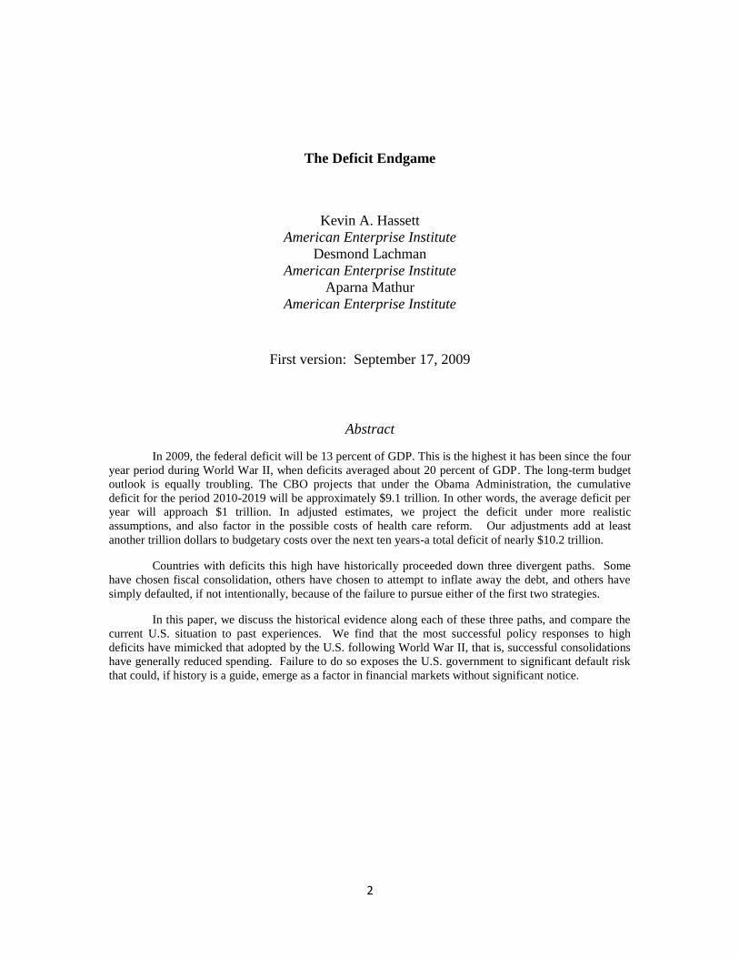
In 2009, the federal deficit will be 13 percent of GDP. This is the highest it has been since the four

year period during World War II, when deficits averaged about 20 percent of GDP. The long-term budget

outlook is equally troubling. The CBO projects that under the Obama Administration, the cumulative

deficit for the period 2010-2019 will be approximately $9.1 trillion. In other words, the average deficit per

year will approach $1 trillion. In adjusted estimates, we project the deficit under more realistic

assumptions, and also factor in the possible costs of health care reform. Our adjustments add at least

another trillion dollars to budgetary costs over the next ten years-a total deficit of nearly $10.2 trillion.

Countries with deficits this high have historically proceeded down three divergent paths. Some

have chosen fiscal consolidation, others have chosen to attempt to inflate away the debt, and others have

simply defaulted, if not intentionally, because of the failure to pursue either of the first two strategies.

In this paper, we discuss the historical evidence along each of these three paths, and compare the

current U.S. situation to past experiences. We find that the most successful policy responses to high

deficits have mimicked that adopted by the U.S. following World War II, that is, successful consolidations

have generally reduced spending. Failure to do so exposes the U.S. government to significant default risk

that could, if history is a guide, emerge as a factor in financial markets without significant notice.

3

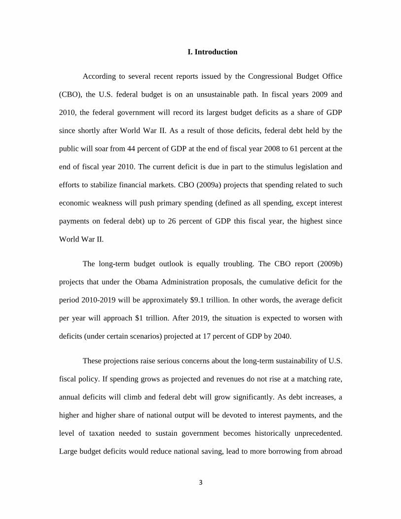
I. Introduction

According to several recent reports issued by the Congressional Budget Office

(CBO), the U.S. federal budget is on an unsustainable path. In fiscal years 2009 and

2010, the federal government will record its largest budget deficits as a share of GDP

since shortly after World War II. As a result of those deficits, federal debt held by the

public will soar from 44 percent of GDP at the end of fiscal year 2008 to 61 percent at the

end of fiscal year 2010. The current deficit is due in part to the stimulus legislation and

efforts to stabilize financial markets. CBO (2009a) projects that spending related to such

economic weakness will push primary spending (defined as all spending, except interest

payments on federal debt) up to 26 percent of GDP this fiscal year, the highest since

World War II.

The long-term budget outlook is equally troubling. The CBO report (2009b)

projects that under the Obama Administration proposals, the cumulative deficit for the

period 2010-2019 will be approximately $9.1 trillion. In other words, the average deficit

per year will approach $1 trillion. After 2019, the situation is expected to worsen with

deficits (under certain scenarios) projected at 17 percent of GDP by 2040.

These projections raise serious concerns about the long-term sustainability of U.S.

fiscal policy. If spending grows as projected and revenues do not rise at a matching rate,

annual deficits will climb and federal debt will grow significantly. As debt increases, a

higher and higher share of national output will be devoted to interest payments, and the

level of taxation needed to sustain government becomes historically unprecedented.

Large budget deficits would reduce national saving, lead to more borrowing from abroad

4

and also lower domestic investment. If such a path is to be averted, then changing policy

sooner reduces the size of the problem significantly.

In this paper, we provide an overview of the current fiscal situation using

projections from the CBO, and make adjustment to account for likely deviations from

CBO baselines. Our calculations suggest that the U.S. fiscal situation is comparable to

that experienced shortly after World War II. As that fiscal hole was filled relatively

quickly, we review policy actions taken at that time and discuss their feasibility today.

We then explore policy actions taken by other countries in similar situations, and evaluate

the economic costs associated with different strategies.

II. The Fiscal Situation

As a starting point, we provide projections of federal revenues, spending and debt

levels from the June 2009 CBO report titled the Long-Term Budget Outlook. These are

long-term projections through 2080 (shown up until 2040 in this paper in Table 1) under

two different assumptions about federal laws and policies. The first set of assumptions

forms the basis for the ―extended baseline scenario‖. This adheres most closely to current

law, following CBO‘s 10-year baseline budget projections and then extending the

baseline concept beyond that 10-year window.1 The second set of assumptions leads to

the ―alternative fiscal scenario‖. This scenario deviates from CBO‘s baseline even during

the next 10 years because it incorporates some policy changes that are widely expected to

1 CBO‘s baseline is a benchmark for measuring the budgetary effects of proposed changes in federal

revenues or spending. It comprises projections of budget authority, outlays, revenues, and the deficit or

surplus calculated according to rules set forth in the Balanced Budget and Emergency Deficit Control Act

of 1985. Those projections are not intended to be predictions of future budgetary outcomes; rather, they

represent CBO‘s best judgment of how economic and other factors would affect federal revenues and

spending if current laws and policies did not change.

5

occur and that policymakers have regularly made in the past. For instance, under the

alternative fiscal scenario, tax provisions in JGTRRA and EGTRRA are extended and

AMT parameters are indexed for inflation after 2009. Also, Medicare physician payment

rates grow with the Medicare economic index rather than at the lower growth rates

scheduled under the sustainable growth rate mechanism. In contrast, the extended-

baseline scenario assumes that the Bush tax cuts will be allowed to expire as under

current law, that the AMT will cover a larger and larger number of people (more than 40

million households by 2017 (Tax Policy Center 2009) and that Medicare‘s sustainable

growth rate mechanism will reduce payment rates for physicians by 21 percent in 2010

and then by a further 4 percent or 5 percent annually for at least the next few years.

However, the extended baseline scenarios are unrealistic. Under the President‘s budget,

many of the tax cuts have been extended and the AMT has been indexed for inflation.

Further, since 2003, the Congress has acted to prevent reductions in Medicare payments

to physicians. For all of these reasons, many budget analysts believe that the alternative

fiscal scenario presents a more realistic picture of the nation‘s underlying fiscal policy

than the extended-baseline scenario does.

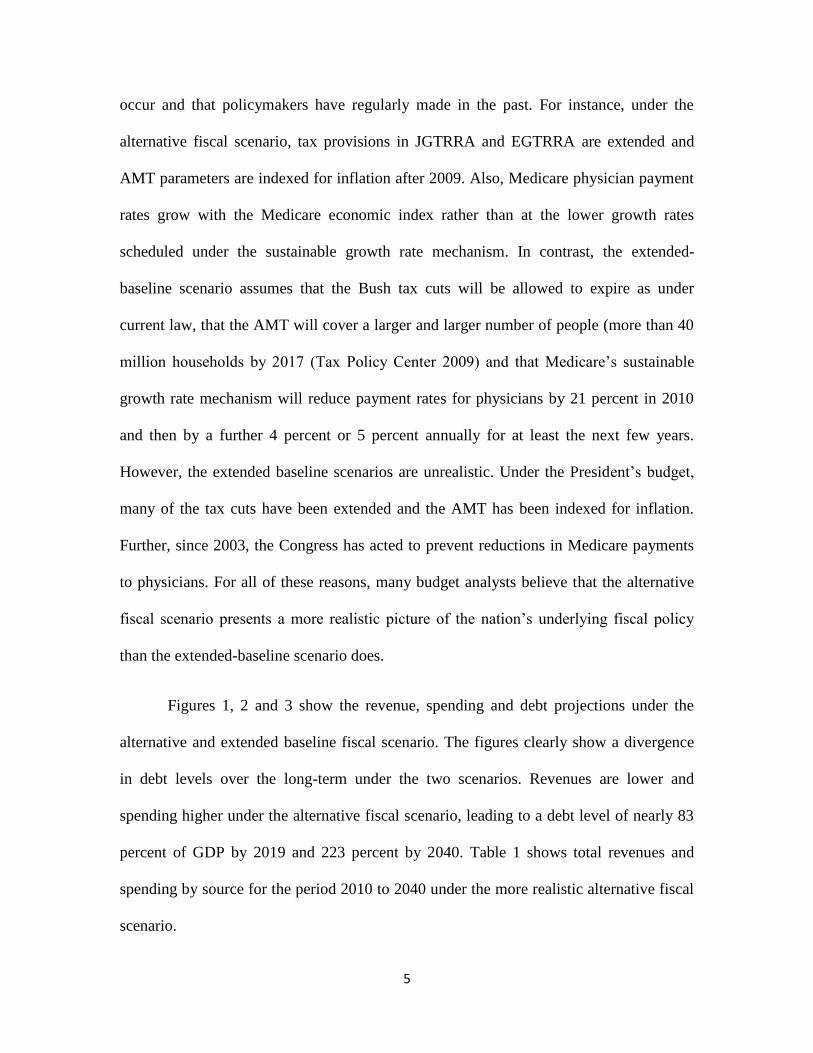
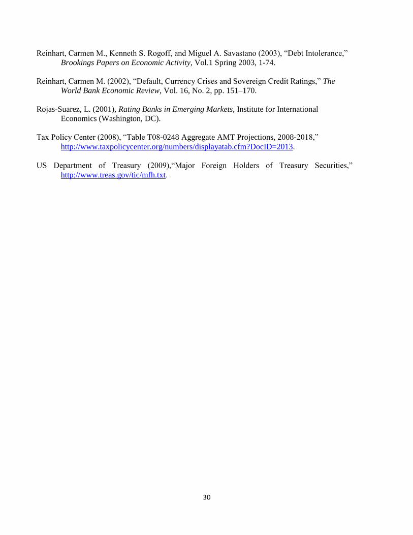
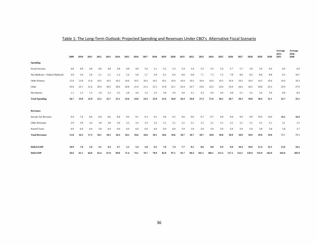
Figures 1, 2 and 3 show the revenue, spending and debt projections under the

alternative and extended baseline fiscal scenario. The figures clearly show a divergence

in debt levels over the long-term under the two scenarios. Revenues are lower and

spending higher under the alternative fiscal scenario, leading to a debt level of nearly 83

percent of GDP by 2019 and 223 percent by 2040. Table 1 shows total revenues and

spending by source for the period 2010 to 2040 under the more realistic alternative fiscal

scenario.

6

Another way to measure the federal government‘s financial status is the fiscal

gap. This represents the extent to which the government would need to immediately and

permanently raise tax revenues, cut spending, or use some mix of both to make the

government‘s debt the same size (relative to the size of the economy) at the end of that

period as it was at the beginning. Under the alternative fiscal scenario, the fiscal gap is

5.4 percent of GDP over the next 25 years and 8.1 percent over the next 75 years. In other

words, under that scenario (ignoring the effects of debt on economic growth), an

immediate and permanent reduction in spending or an immediate and permanent increase

in revenues equal to 8.1 percent of GDP would be needed to create a sustainable fiscal

path for the next three quarters of a century. If the policy change was not immediate, the

required percentage would be greater.

Note that even the projections under the alternative fiscal scenario may be

somewhat conservative. This is because the CBO assumes that all economic variables,

such as economic growth and real interest rates, are unaffected by rising federal debt

levels. However, if debt actually increased as projected under either scenario, interest

rates would be higher to some extent than otherwise and economic growth would be

slower. The rising debt would reduce the size of the domestic capital stock (businesses‘

equipment and structures as well as housing) and decrease U.S. ownership of assets in

other countries while increasing foreign ownership of assets in the United States. Those

changes would slow the growth of gross national product (GNP) and, as the debt burden

rose, could eventually lead to a decline in economic output.

The effects would be most striking under the alternative fiscal scenario. In CBO‘s

estimation, the increase in debt under that scenario would reduce the capital stock by

7

more than 20 percent and real GNP by 9 percent in 2035, compared with the levels that

would occur if the debt remained roughly at its current size relative to the economy.

Under the extended-baseline scenario, federal debt would be less threatening in the near

term but would lead to significant economic harm in the long run. Those economic

effects mean that actual fiscal pressures under current laws and policies would be even

greater than CBO‘s long-term budget projections suggest, because slower growth would

limit revenues and a smaller capital stock would imply higher interest rates on

government debt and other financial instruments.

Note that these long-term projections capture broad changes that are expected to

occur over the course of the next few decades. For instance, while they model the

extension of EGTRRA and JGTRRA, they do not specifically model the effect of

extending the tax cuts only to the lower income groups. The Administration‘s budget

however makes the distinction that for taxpayers with income above certain levels, the

income tax rates of 36 percent and 39.6 percent scheduled to go into effect in 2011 under

current law would apply. For the remaining taxpayers, tax rates would be at 2010 levels

specified in EGTRRA. To understand the impact that these specific proposals would have

on the fiscal deficit, we next turn to an analysis of the Administration‘s budget proposals.

II.A. The Administration‘s Budget

The CBO provided an analysis of the Administration‘s budget following the

release of the full budget proposal in May for fiscal year 2010. The CBO (2009b)

baseline projections and the effect of the President‘s proposal on the baseline are shown

in Table 2. Under the President‘s policies, the deficit in 2009 will equal $1.8 trillion or 13

percent of GDP. This is higher than the CBO baseline estimate (under current law) by

8

$157 billion due to the additional spending by the government on stabilizing financial

markets and the ongoing military operations in Iraq and Afghanistan. The cumulative

deficit over the 2010-2019 period would equal $9.1 trillion, more than double the

cumulative deficit projected under the CBO baseline.

The differences under the current law assumptions of the CBO baseline and the

President‘s budget arise from several sources. Of the various revenue proposals,

modifying and extending provisions of JGTRRA and EGTRRA would have the largest

effect, reducing revenues by $1.9 trillion. Note that the baseline assumes that these

provisions will expire at the end of 2010. In addition, indexing the AMT for inflation

would reduce revenues by $447 billion and the proposal to permanently extend the

Making Work Pay Credit would reduce them by $381 billion. The projections also

assume that the proposal to reduce greenhouse gas emissions would raise an estimated

$632 billion in revenues between 2012 and 2019. Further, the international tax proposals

would raise revenues by $161 billion.

Finally, the budget assumes that the cost of health care reform is zero. Health care

reform benefits may be a combination of revenue reductions and spending increases and

are assumed to exactly offset the savings dedicated to the proposal on both the revenue

and outlay sides of the budget.

Assuming that all of the President‘s proposals are eventually adopted, the CBO

estimates that over the next decade, the budget deficit would average about 5.2 percent of

GDP. The 2009 deficit is projected to be 13 percent with a subsequent decline to 3.9

percent by 2013 and then an increase to 5.5 percent by 2019. The increase is primarily the

result of rising health care spending and debt-service costs. As a result, public debt would

9

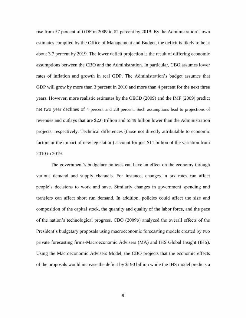
rise from 57 percent of GDP in 2009 to 82 percent by 2019. By the Administration‘s own

estimates compiled by the Office of Management and Budget, the deficit is likely to be at

about 3.7 percent by 2019. The lower deficit projection is the result of differing economic

assumptions between the CBO and the Administration. In particular, CBO assumes lower

rates of inflation and growth in real GDP. The Administration‘s budget assumes that

GDP will grow by more than 3 percent in 2010 and more than 4 percent for the next three

years. However, more realistic estimates by the OECD (2009) and the IMF (2009) predict

net two year declines of 4 percent and 2.8 percent. Such assumptions lead to projections of

revenues and outlays that are $2.6 trillion and $549 billion lower than the Administration

projects, respectively. Technical differences (those not directly attributable to economic

factors or the impact of new legislation) account for just $11 billion of the variation from

2010 to 2019.

The government‘s budgetary policies can have an effect on the economy through

various demand and supply channels. For instance, changes in tax rates can affect

people‘s decisions to work and save. Similarly changes in government spending and

transfers can affect short run demand. In addition, policies could affect the size and

composition of the capital stock, the quantity and quality of the labor force, and the pace

of the nation‘s technological progress. CBO (2009b) analyzed the overall effects of the

President‘s budgetary proposals using macroeconomic forecasting models created by two

private forecasting firms-Macroeconomic Advisers (MA) and IHS Global Insight (IHS).

Using the Macroeconomic Advisers Model, the CBO projects that the economic effects

of the proposals would increase the deficit by $190 billion while the IHS model predicts a

10

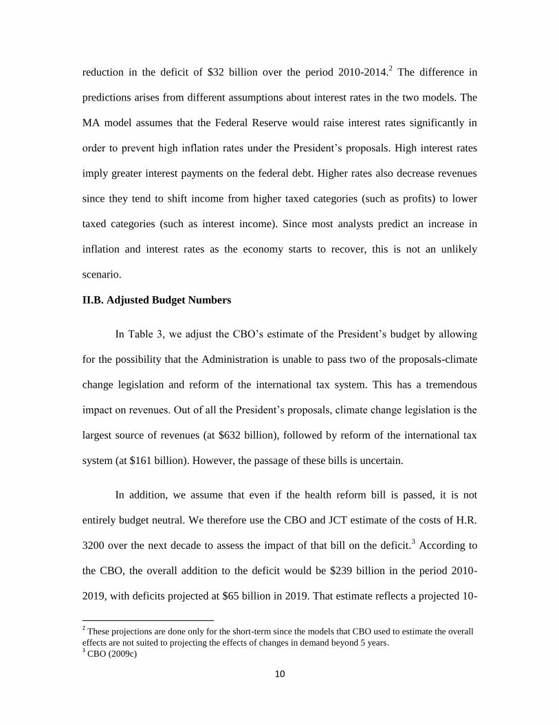
reduction in the deficit of $32 billion over the period 2010-2014.2 The difference in

predictions arises from different assumptions about interest rates in the two models. The

MA model assumes that the Federal Reserve would raise interest rates significantly in

order to prevent high inflation rates under the President‘s proposals. High interest rates

imply greater interest payments on the federal debt. Higher rates also decrease revenues

since they tend to shift income from higher taxed categories (such as profits) to lower

taxed categories (such as interest income). Since most analysts predict an increase in

inflation and interest rates as the economy starts to recover, this is not an unlikely

scenario.

II.B. Adjusted Budget Numbers

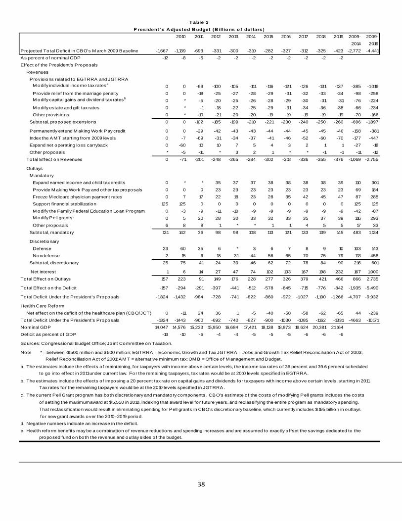
In Table 3, we adjust the CBO‘s estimate of the President‘s budget by allowing

for the possibility that the Administration is unable to pass two of the proposals-climate

change legislation and reform of the international tax system. This has a tremendous

impact on revenues. Out of all the President‘s proposals, climate change legislation is the

largest source of revenues (at $632 billion), followed by reform of the international tax

system (at $161 billion). However, the passage of these bills is uncertain.

In addition, we assume that even if the health reform bill is passed, it is not

entirely budget neutral. We therefore use the CBO and JCT estimate of the costs of H.R.

3200 over the next decade to assess the impact of that bill on the deficit.3 According to

the CBO, the overall addition to the deficit would be $239 billion in the period 2010-

2019, with deficits projected at $65 billion in 2019. That estimate reflects a projected 10-

2 These projections are done only for the short-term since the models that CBO used to estimate the overall

effects are not suited to projecting the effects of changes in demand beyond 5 years. 3 CBO (2009c)

11

year cost of the bill‘s insurance coverage provisions of $1,042 billion, partly offset by net

spending changes that CBO estimates could save $219 billion over the same period and

by revenue provisions that JCT estimates would increase federal revenues by about $583

billion.

Under this adjusted estimate (accounting for all three possibilities), the total

deficit for 2010-2019 increases to $10.1 trillion i.e. an additional $1 trillion would be

added to the deficit. In 2019, the deficit would be close to 6 percent of GDP. Even if we

assume that health care reform is in fact budget neutral, the cumulative deficit for 2019

would still be $9.9 trillion.

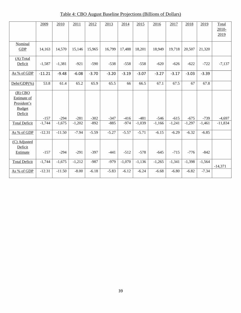
At the time of writing this paper, the CBO came out with a revised version of its

baseline estimate of the deficit. The August (CBO, 2009e) baseline projects a marginally

lower deficit for 2009 of $1.58 trillion. However, over the entire 2010-2019 period, the

deficit is expected to be higher by nearly $2.7 trillion relative to the March estimates. The

report however does not revise the CBO‘s estimate of the President‘s budget. Therefore,

in Table 4, we present the projected deficits using the August baseline and the June

estimates of the President‘s budgetary proposals on the deficits. We also incorporate our

adjusted budget estimates and show what deficits would look like under the scenario of

high health care costs and no revenues from climate change and international tax reform.

As per the new CBO baseline, the deficit in 2009 will be approximately 11 percent of

GDP. However, it will decline to 3.4 percent by 2019. Debt held by the public is

projected to exceed 61 percent of GDP by the end of next year, which is the highest level

since 1952, and reach 68 percent by the end of 2019. That accumulating federal debt,

coupled with rising interest rates, would lead to a near tripling of net interest payments

12

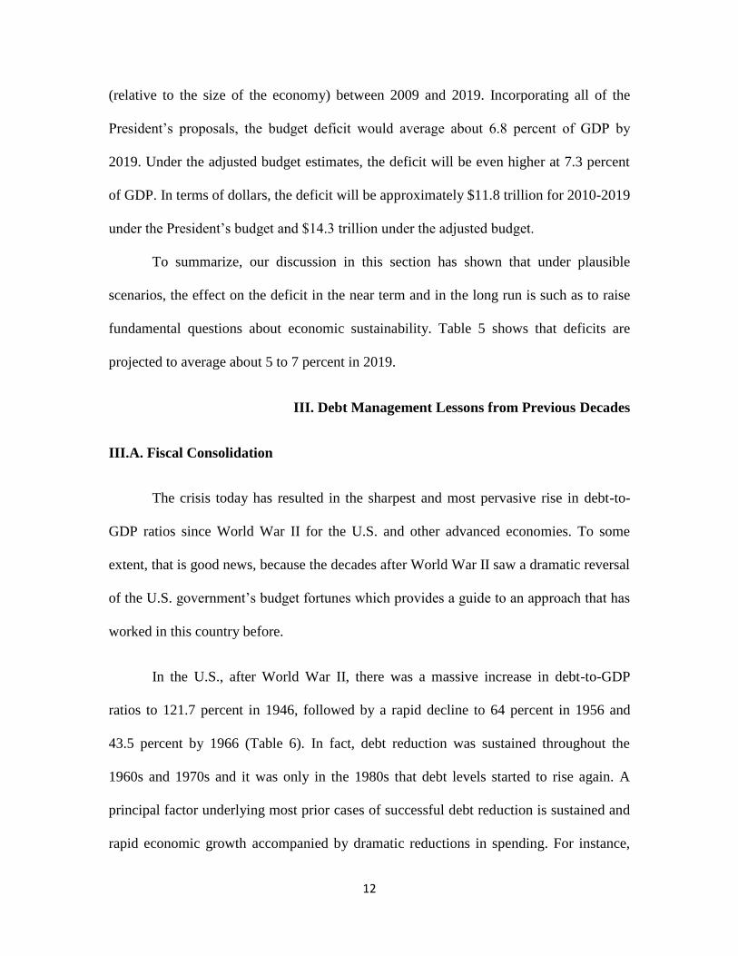
(relative to the size of the economy) between 2009 and 2019. Incorporating all of the

President‘s proposals, the budget deficit would average about 6.8 percent of GDP by

2019. Under the adjusted budget estimates, the deficit will be even higher at 7.3 percent

of GDP. In terms of dollars, the deficit will be approximately $11.8 trillion for 2010-2019

under the President‘s budget and $14.3 trillion under the adjusted budget.

To summarize, our discussion in this section has shown that under plausible

scenarios, the effect on the deficit in the near term and in the long run is such as to raise

fundamental questions about economic sustainability. Table 5 shows that deficits are

projected to average about 5 to 7 percent in 2019.

III. Debt Management Lessons from Previous Decades

III.A. Fiscal Consolidation

The crisis today has resulted in the sharpest and most pervasive rise in debt-to-

GDP ratios since World War II for the U.S. and other advanced economies. To some

extent, that is good news, because the decades after World War II saw a dramatic reversal

of the U.S. government‘s budget fortunes which provides a guide to an approach that has

worked in this country before.

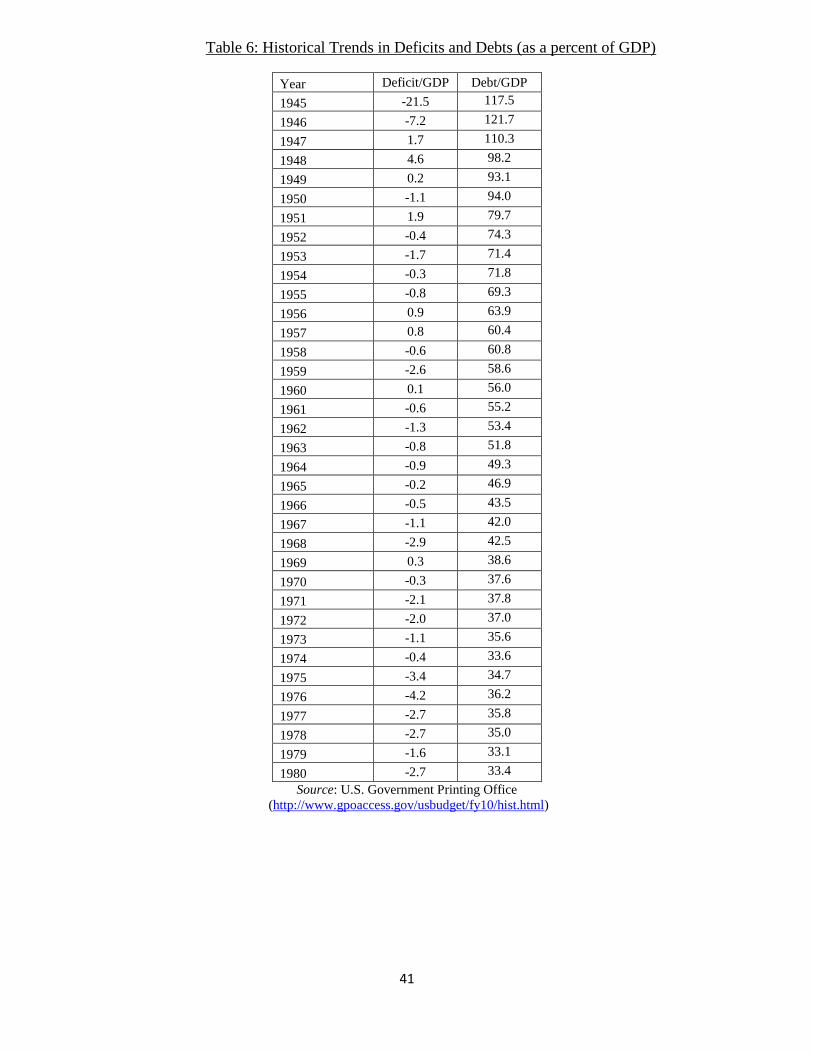
In the U.S., after World War II, there was a massive increase in debt-to-GDP

ratios to 121.7 percent in 1946, followed by a rapid decline to 64 percent in 1956 and

43.5 percent by 1966 (Table 6). In fact, debt reduction was sustained throughout the

1960s and 1970s and it was only in the 1980s that debt levels started to rise again. A

principal factor underlying most prior cases of successful debt reduction is sustained and

rapid economic growth accompanied by dramatic reductions in spending. For instance,

13

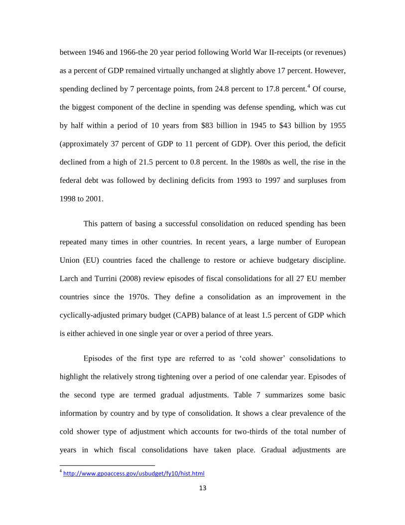
between 1946 and 1966-the 20 year period following World War II-receipts (or revenues)

as a percent of GDP remained virtually unchanged at slightly above 17 percent. However,

spending declined by 7 percentage points, from 24.8 percent to 17.8 percent.4 Of course,

the biggest component of the decline in spending was defense spending, which was cut

by half within a period of 10 years from $83 billion in 1945 to $43 billion by 1955

(approximately 37 percent of GDP to 11 percent of GDP). Over this period, the deficit

declined from a high of 21.5 percent to 0.8 percent. In the 1980s as well, the rise in the

federal debt was followed by declining deficits from 1993 to 1997 and surpluses from

1998 to 2001.

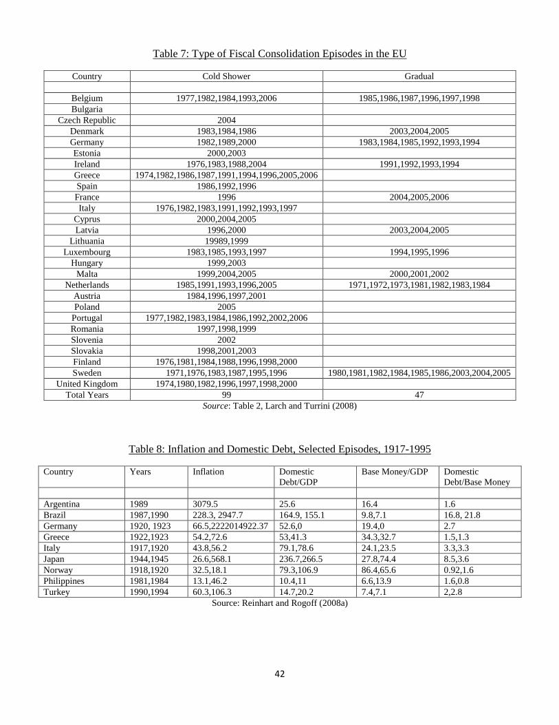
This pattern of basing a successful consolidation on reduced spending has been

repeated many times in other countries. In recent years, a large number of European

Union (EU) countries faced the challenge to restore or achieve budgetary discipline.

Larch and Turrini (2008) review episodes of fiscal consolidations for all 27 EU member

countries since the 1970s. They define a consolidation as an improvement in the

cyclically-adjusted primary budget (CAPB) balance of at least 1.5 percent of GDP which

is either achieved in one single year or over a period of three years.

Episodes of the first type are referred to as ‗cold shower‘ consolidations to

highlight the relatively strong tightening over a period of one calendar year. Episodes of

the second type are termed gradual adjustments. Table 7 summarizes some basic

information by country and by type of consolidation. It shows a clear prevalence of the

cold shower type of adjustment which accounts for two-thirds of the total number of

years in which fiscal consolidations have taken place. Gradual adjustments are

4 http://www.gpoaccess.gov/usbudget/fy10/hist.html

14

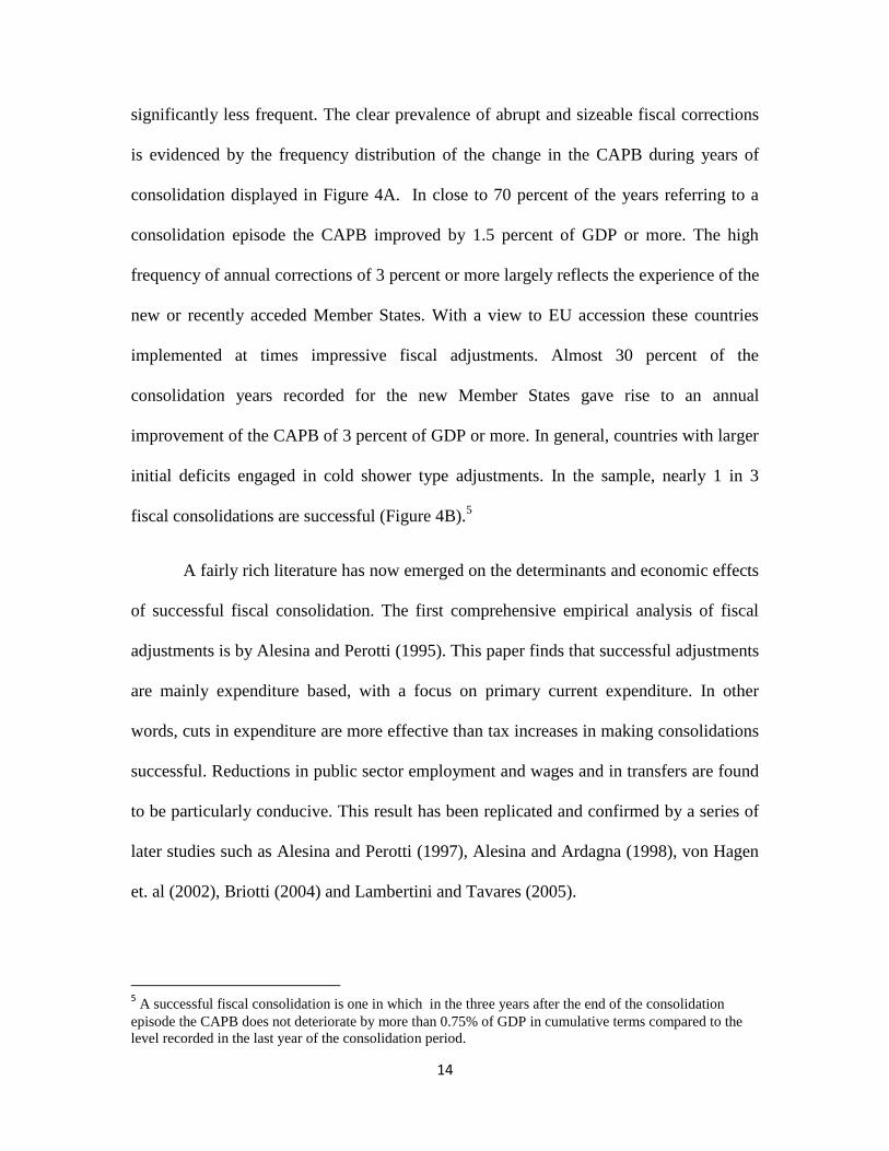
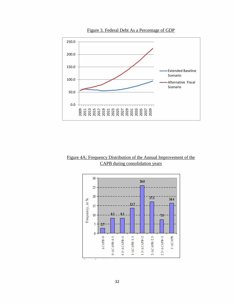
significantly less frequent. The clear prevalence of abrupt and sizeable fiscal corrections

is evidenced by the frequency distribution of the change in the CAPB during years of

consolidation displayed in Figure 4A. In close to 70 percent of the years referring to a

consolidation episode the CAPB improved by 1.5 percent of GDP or more. The high

frequency of annual corrections of 3 percent or more largely reflects the experience of the

new or recently acceded Member States. With a view to EU accession these countries

implemented at times impressive fiscal adjustments. Almost 30 percent of the

consolidation years recorded for the new Member States gave rise to an annual

improvement of the CAPB of 3 percent of GDP or more. In general, countries with larger

initial deficits engaged in cold shower type adjustments. In the sample, nearly 1 in 3

fiscal consolidations are successful (Figure 4B).5

A fairly rich literature has now emerged on the determinants and economic effects

of successful fiscal consolidation. The first comprehensive empirical analysis of fiscal

adjustments is by Alesina and Perotti (1995). This paper finds that successful adjustments

are mainly expenditure based, with a focus on primary current expenditure. In other

words, cuts in expenditure are more effective than tax increases in making consolidations

successful. Reductions in public sector employment and wages and in transfers are found

to be particularly conducive. This result has been replicated and confirmed by a series of

later studies such as Alesina and Perotti (1997), Alesina and Ardagna (1998), von Hagen

et. al (2002), Briotti (2004) and Lambertini and Tavares (2005).

5 A successful fiscal consolidation is one in which in the three years after the end of the consolidation

episode the CAPB does not deteriorate by more than 0.75% of GDP in cumulative terms compared to the

level recorded in the last year of the consolidation period.

15

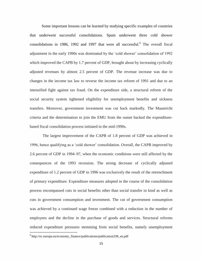
Some important lessons can be learned by studying specific examples of countries

that underwent successful consolidations. Spain underwent three cold shower

consolidations in 1986, 1992 and 1997 that were all successful.6 The overall fiscal

adjustment in the early 1990s was dominated by the ‗cold shower‘ consolidation of 1992

which improved the CAPB by 1.7 percent of GDP, brought about by increasing cyclically

adjusted revenues by almost 2.5 percent of GDP. The revenue increase was due to

changes in the income tax law to reverse the income tax reform of 1991 and due to an

intensified fight against tax fraud. On the expenditure side, a structural reform of the

social security system tightened eligibility for unemployment benefits and sickness

transfers. Moreover, government investment was cut back markedly. The Maastricht

criteria and the determination to join the EMU from the outset backed the expenditure-

based fiscal consolidation process initiated in the mid-1990s.

The largest improvement of the CAPB of 1.8 percent of GDP was achieved in

1996, hence qualifying as a ‗cold shower‘ consolidation. Overall, the CAPB improved by

2.6 percent of GDP in 1994–97, when the economic conditions were still affected by the

consequences of the 1993 recession. The strong decrease of cyclically adjusted

expenditure of 1.2 percent of GDP in 1996 was exclusively the result of the retrenchment

of primary expenditure. Expenditure measures adopted in the course of the consolidation

process encompassed cuts in social benefits other than social transfer in kind as well as

cuts in government consumption and investment. The cut of government consumption

was achieved by a continued wage freeze combined with a reduction in the number of

employees and the decline in the purchase of goods and services. Structural reforms

reduced expenditure pressures stemming from social benefits, namely unemployment

6 http://ec.europa.eu/economy_finance/publications/publication338_en.pdf

16

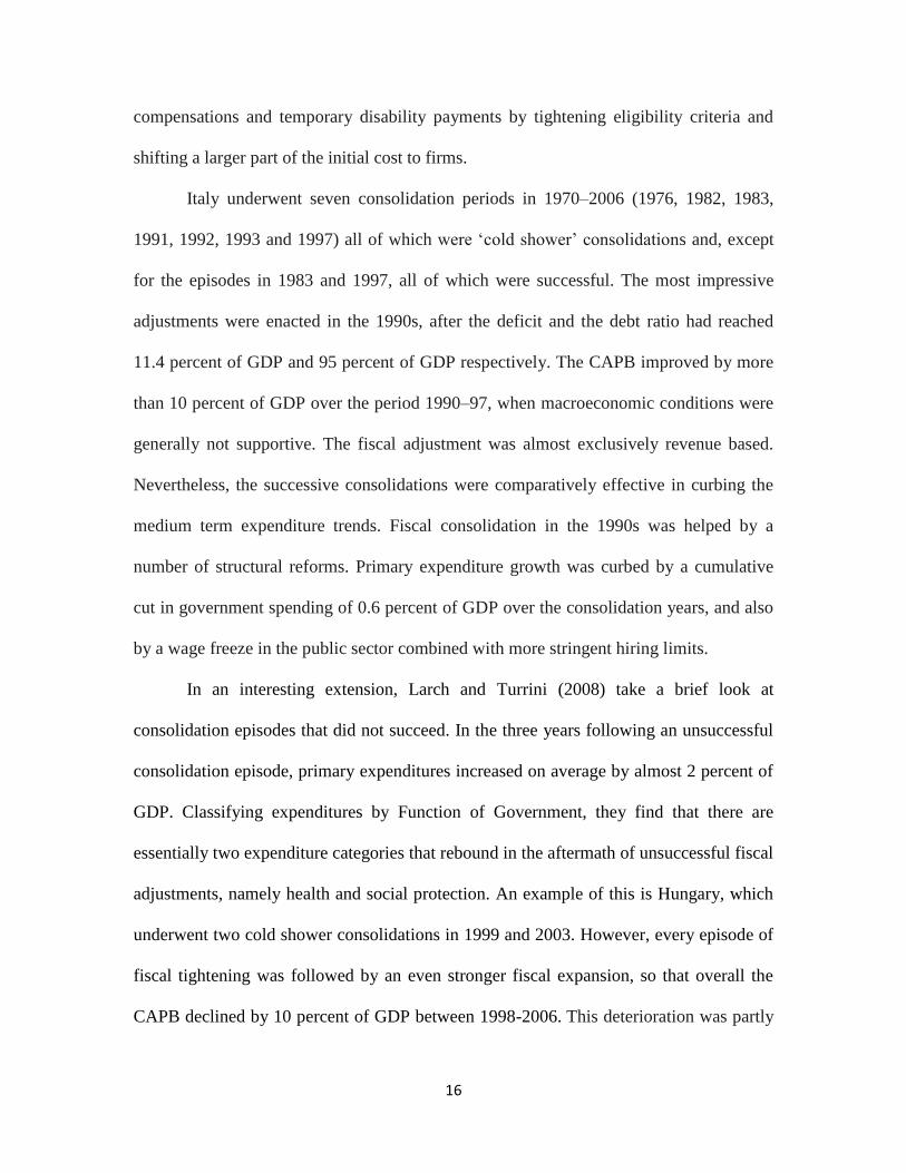
compensations and temporary disability payments by tightening eligibility criteria and

shifting a larger part of the initial cost to firms.

Italy underwent seven consolidation periods in 1970–2006 (1976, 1982, 1983,

1991, 1992, 1993 and 1997) all of which were ‗cold shower‘ consolidations and, except

for the episodes in 1983 and 1997, all of which were successful. The most impressive

adjustments were enacted in the 1990s, after the deficit and the debt ratio had reached

11.4 percent of GDP and 95 percent of GDP respectively. The CAPB improved by more

than 10 percent of GDP over the period 1990–97, when macroeconomic conditions were

generally not supportive. The fiscal adjustment was almost exclusively revenue based.

Nevertheless, the successive consolidations were comparatively effective in curbing the

medium term expenditure trends. Fiscal consolidation in the 1990s was helped by a

number of structural reforms. Primary expenditure growth was curbed by a cumulative

cut in government spending of 0.6 percent of GDP over the consolidation years, and also

by a wage freeze in the public sector combined with more stringent hiring limits.

In an interesting extension, Larch and Turrini (2008) take a brief look at

consolidation episodes that did not succeed. In the three years following an unsuccessful

consolidation episode, primary expenditures increased on average by almost 2 percent of

GDP. Classifying expenditures by Function of Government, they find that there are

essentially two expenditure categories that rebound in the aftermath of unsuccessful fiscal

adjustments, namely health and social protection. An example of this is Hungary, which

underwent two cold shower consolidations in 1999 and 2003. However, every episode of

fiscal tightening was followed by an even stronger fiscal expansion, so that overall the

CAPB declined by 10 percent of GDP between 1998-2006. This deterioration was partly

17

due to the continued high increases of public sector wages and social benefit spending as

well as a revenue loss due to the exemption of old-age pension from the calculation of

taxable income.

This should serve as a warning for economies embarking on such consolidations

today since these social expenditure categories typically represent a large fraction of the

budget and will bear the budgetary impact of an ageing population.

While the one clear lesson from prior experiences of successful debt reduction is

that of restraining spending, what is less clear is how to go about doing so in today‘s

American economy. Since the 1960s, the composition of spending in the U.S. and other

industrialized economies has shifted towards social welfare entitlements and away from

defense. 7

For a time, the costs of these social welfare programs were financed through

budgetary growth and transfers from other parts of the budget, such as defense. Over

time, however, these programs have grown tremendously. According to the CBO

(2009a), spending on the three largest entitlement programs-Medicare, Medicaid and

Social Security-has grown from 25 percent in 1975 to 45 percent today. Over the next 75

years, total spending on these programs will grow even more due to population aging and

higher health care costs per person. CBO (2009a) projects that net federal spending on

Medicare and Medicaid will rise from about 5 percent of GDP in fiscal year 2009 to

about 10 percent in 2035 and over 17 percent in 2080. Spending on Social Security is

projected to rise at a much slower pace, from almost 5 percent of GDP in 2009 to about 6

percent in later years. These projections assume that the programs will continue to pay

7 Ippolito (2003)

18

benefits as currently scheduled even though the trust funds for Medicare and Social

Security are projected to become insolvent at some point in the near future.

Therefore, one obvious starting point for debt reduction is restraining the

spending on these programs. This approach has not been adopted by the current

administration. As we mentioned earlier, the cost of health care reform as estimated by

the CBO and the JCT is approximately another $239 billion over the next decade, but the

costs could easily exceed $1 trillion. The CBO projects that in the absence of specific

constraints on growth, the new spending associated with health care reform would

probably increase over time roughly with the underlying costs of health care and thus

would grow as fast as spending on other federal health care programs.8 From that

perspective, a large-scale expansion of insurance coverage would represent a permanent

increase of roughly 10 percent in the federal budgetary commitment to health care.

It also bears emphasizing that if a reform package achieved ―budget neutrality‖

during its first 10 years, budgetary savings in the long run would not be guaranteed—

even if the package included initial steps toward transforming the delivery and financing

of healthcare that would gain momentum over time. Different reform plans would have

different effects, of course, but two general phenomena could make the long-run

budgetary impact less favorable than the short-run impact: First, an expansion of

insurance coverage would be phased in over time to allow for the creation of new

administrative structures such as insurance exchanges. As a result, the cost of an

expansion during the 2010–2019 period could be a poor indicator of its ultimate cost.

Second, savings generated by policy actions outside of the health care system would

probably not grow as fast as health care spending. Such would be the case for revenues

8 CBO (2009d)

19

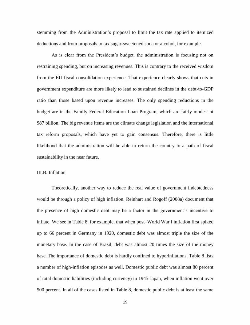
stemming from the Administration‘s proposal to limit the tax rate applied to itemized

deductions and from proposals to tax sugar-sweetened soda or alcohol, for example.

As is clear from the President‘s budget, the administration is focusing not on

restraining spending, but on increasing revenues. This is contrary to the received wisdom

from the EU fiscal consolidation experience. That experience clearly shows that cuts in

government expenditure are more likely to lead to sustained declines in the debt-to-GDP

ratio than those based upon revenue increases. The only spending reductions in the

budget are in the Family Federal Education Loan Program, which are fairly modest at

$87 billion. The big revenue items are the climate change legislation and the international

tax reform proposals, which have yet to gain consensus. Therefore, there is little

likelihood that the administration will be able to return the country to a path of fiscal

sustainability in the near future.

III.B. Inflation

Theoretically, another way to reduce the real value of government indebtedness

would be through a policy of high inflation. Reinhart and Rogoff (2008a) document that

the presence of high domestic debt may be a factor in the government‘s incentive to

inflate. We see in Table 8, for example, that when post–World War I inflation first spiked

up to 66 percent in Germany in 1920, domestic debt was almost triple the size of the

monetary base. In the case of Brazil, debt was almost 20 times the size of the money

base. The importance of domestic debt is hardly confined to hyperinflations. Table 8 lists

a number of high-inflation episodes as well. Domestic public debt was almost 80 percent

of total domestic liabilities (including currency) in 1945 Japan, when inflation went over

500 percent. In all of the cases listed in Table 8, domestic public debt is at least the same

20

order of magnitude as the monetary base (with the exception of Norway in 1918, where it

was slightly below). In the U.S., the monetary base for July 2009 was $1695.7 billion,

while the debt for 2009 is projected to be $7,612 billion.9 Therefore, the debt is

approximately 4.5 times the monetary base. Even if we only focus on domestic debt, the

ratio is higher than 2 i.e the debt in 2009 will be more than twice the monetary base. The

fact that nominal debt is so large compared to the monetary base leads to the risk that the

government may attempt to lower the real value of debt through a spike in inflation.

However, unless the government engineers a sudden and unanticipated

inflationary burst, one would expect that markets would shorten the duration of their debt

holdings and demand higher interest payments on longer dated debt to compensate them

for the risk of inflation. This would imply that inflation would have to rise to very high

levels for an extended period of time to make any dent on the government‘s debt to GDP

ratio.

It is highly questionable whether such a policy is possible in the U.S. The Federal

Reserve has the legal responsibility to provide price stability, and the experience of the

1970s has ingrained in monetary policymakers the view that the economic costs of high

inflation are significant.10

III.C. Debt Default

The final resort of a government unable to meet its debt obligations is default.

Investors‘ perceptions about the likelihood of a U.S. default are captured in the credit

default swap markets. In September 2008, data on these swaps showed that the price of

9 http://research.stlouisfed.org/fred2/series/AMBNS?cid=124

10 The re-appointment of Ben Bernanke as Federal Reserve Chairman makes the adoption of such a policy a

fairly remote possibility.

21

purchasing insurance against default on 5-year senior U.S. treasury debt was around 10

basis points. This rose to 90 basis points in the beginning of this year and is currently at

about 30 basis points. The implied likelihood of default is approximately around 4

percent (Auerbach and Gale, 2009). Hence there has been a visible increase in the

likelihood of a U.S. debt default.

It must be noted that a debt default event need not involve the government putting

a sudden stop to interest payments. The most likely scenario is that the government

arrives at the Treasury auction one day, and finds that there are not enough willing buyers

for it to roll over expiring debts. At that point, the government may have to change the

terms on the expiring debt unilaterally. For instance, in August 1982, the Mexican

government suddenly found itself unable to roll over it‘s private debts. Soon after, other

countries sought rescheduling arrangements, starting the debt crisis of the 1980s.11

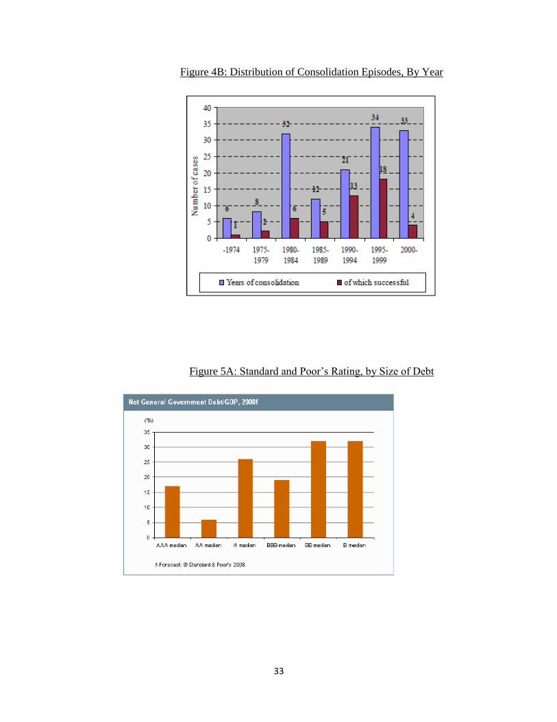
Such a scenario can creep up at any time, and likely would be caused by a sudden

panic. Such a panic might be set off by a dramatic policy change in the U.S., such as

passage of a fiscally irresponsible health reform, or by external events. For instance, the

Standard and Poor‘s charts show that AAA rated countries generally have net public debt

ratios that are below 20 percent of GDP (Figure 5A) and low government deficits (Figure

5B).12

This would suggest that if the U.S. is indeed on the way to a debt ratio of 100

percent and deficits of about 5 or 6 percent of GDP, it could be risking losing its AAA

rating. This could trigger a panic as investors may try to move away from U.S.

government bonds to other assets.13

11

http://www.econlib.org/library/Enc1/ThirdWorldDebt.html 12

http://www.ratings.com/spf/pdf/fixedincome/KR_sovereign_APrimer_Eng.pdf 13 The predictive power of credit ratings for currency crisis and sovereign default is however, surprisingly

poor. This became evident in the Asian crisis or, more recently, in the Argentinean crisis. Systematic

22

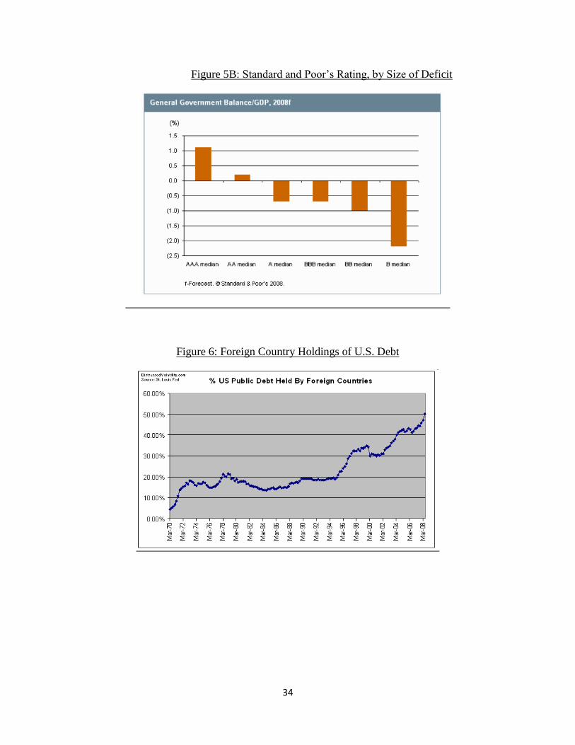
A U.S. government default would impose huge costs on the economy and cause a

breakdown in globalization as foreign governments would likely retaliate against a U.S.

government reneging on its obligations. This is particularly problematic since the

proportion of the government deficit financed by foreigners has already increased to an

unprecedented 50 percent (Figure 6). Foreign central banks alone are presently sitting on

$2.3 trillion in U.S. Treasury bonds, out of a total outstanding debt of more than $7

trillion.14

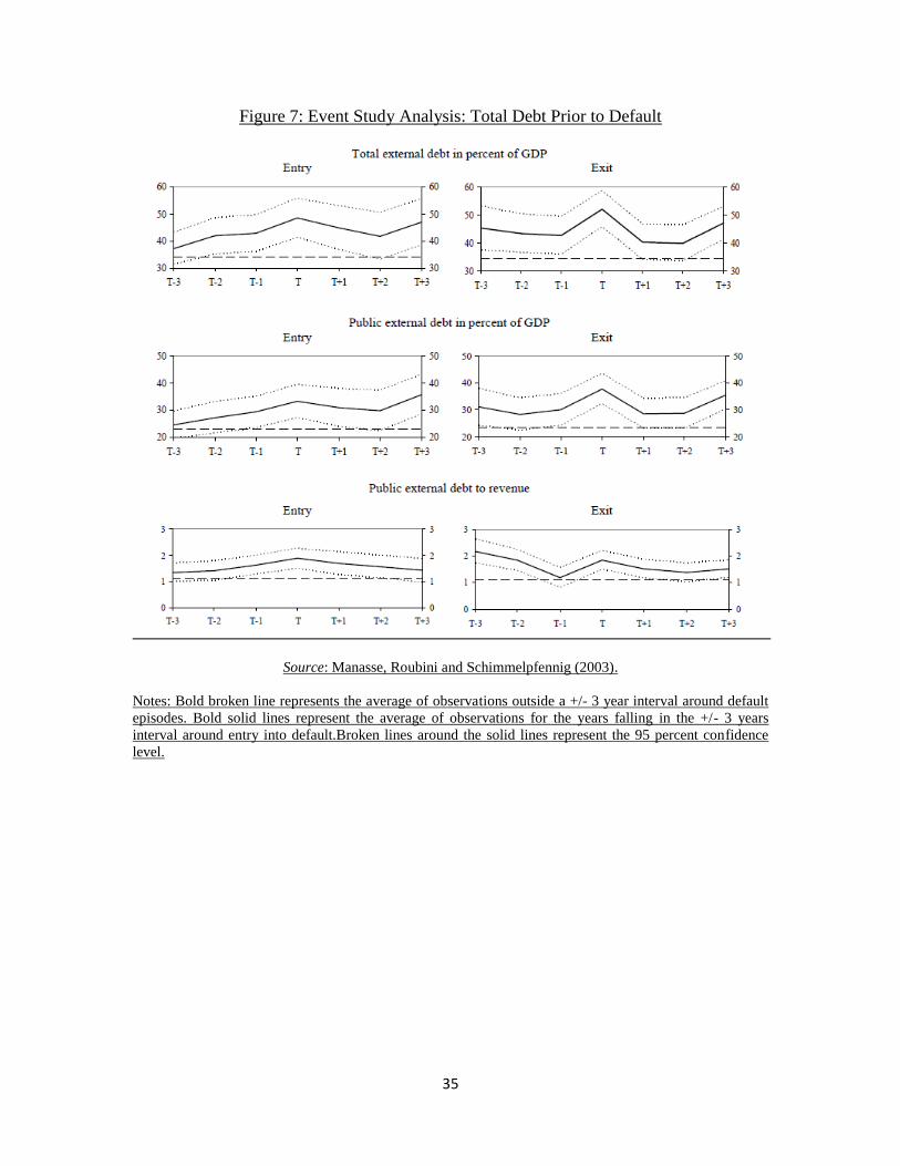
Manasse, Roubini and Shennelpfennig (2003) show that this build up in

government debt, particularly external debt, is symptomatic of previous sovereign default

episodes. Using data on macroeconomic variables, political and institutional variables as

well as measures of solvency for 47 countries, the paper concludes that high levels of

foreign debt (relative to GDP) increase the probability of default. Looking at the period

prior to the default, there is an increase in external debt measures in the year before the

crisis and also in the years of the crisis. On average, external debt to GDP averages about

54.7 percent when moving into a crisis year, and 71.4 percent in a crisis year. These

numbers are fairly close to currently projected U.S. debt levels, raising the risk of

sovereign default. In particular, in June 2009, total external debt (which includes public

or government debt as well as the debt owed by residents to all foreigners) was calculated

at $13.4 trillion or more than 90 percent of projected GDP.15

Of this, total public external

evidence in this regard is presented in Reinhart (2002); Rojas-Suarez (2001); and Larrain, Reisen, and von

Maltzan (1997). Related studies have analyzed the determinants of credits ratings. Some studies test

whether credit ratings are significantly correlated with a range of economic fundamentals. Measures of

external debt, default history, as well as other macroeconomic and political variables are found to be

correlated with default/debt-crisis events (e.g., Haque, Nelson, and Mathieson, 1998; Cantor and Packer,

1996; and Lee, 1993). 14

http://www.treas.gov/tic/mfh.txt

15 http://www.treas.gov/tic/debta309.html

23

debt (which includes only the external debt obligations of the public sector) was

approximately $3.4 trillion.16

Therefore, public external debt to GDP in 2009 will be

close to 24 percent and the ratio of public external debt to revenues will be 1.62. In

Figure 7, reproduced from this same paper, public external debt to GDP averaged about

36 percent and the ratio of public external debt to revenues was 1.9 in the year before the

crisis. Therefore, by all relevant debt indicators, the U.S. fiscal scenario will soon

approximate the economic scenario for countries on the verge of a sovereign debt default.

Recent research by Reinhart and Rogoff (2008b) on the long run history of

external sovereign debt defaults is sobering. In this NBER Working Paper, they show that

sovereign debt default is far from an isolated event. Over the longer sweep of history

there have been fairly regular episodes where all too many sovereign governments have

resorted to defaulting or restructuring their government debt. By their count, over 40

percent of countries did so in the aftermath of the Great Depression and over 30 percent

did the same in the aftermath of the 1980-82 global economic recession. Two further

regularities found by Reinhart and Rogoff (2008b) would seem to be particularly

pertinent to today‘s U.S. context. The first is that those countries most at risk of

defaulting on their government debts were those that were overly dependent on capital

flows from abroad to finance their government deficits. The second was that sovereign

debt default or restructuring tended to be highly disruptive to economic performance in

general and to inflation performance in particular.

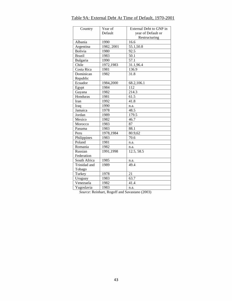
This latter issue is explored more fully in Reinhart, Rogoff and Savastano (2003).

The paper explores the idea of debt intolerance defined as some countries‘ inability to

handle debt levels that would seem manageable by advanced country standards. Such

16

http://www.treas.gov/tic/mfh.txt

24

countries typically experience serial defaults. For instance, Spain defaulted 13 times

between 1500 and 1900, Venezuela has defaulted nine times since the 1800s and more

recently, Argentina has defaulted five times on its external debts. This vicious cycle of

defaults is perpetuated by the lasting damage that defaults can impose on a country‘s

financial system and the linkages between domestic and foreign markets. Weak financial

structures in turn reduce the penalty to default, thereby leading to more defaults at

relatively low debt levels. That explains why defaults occur at debt-to GDP ratios that are

not excessively high by advanced country standards. Table 9A, reproduced from this

paper, shows all episodes of default or debt restructuring during 1970-2001 for middle

income emerging economies. On average, about half of the defaults occurred at external

debt to GNP ratios that were lower than 60 percent and about 17 percent occurred at debt

levels lower than 40 percent of GDP. These are sobering statistics since in 2009 U.S. total

external debt to GNP is estimated to be at 90 percent, while public external debt to GNP

is likely to reach 24 percent.17

Therefore, to avoid long-term damage to the U.S. banking

and financial systems and escape the spiral of future defaults, the country needs to go to

great lengths to avoid this first default.

In another paper, Reinhart and Rogoff (2008a) suggest that the focus on external

debts in explaining sovereign defaults is somewhat misplaced. Often countries default on

their external obligations at very low thresholds. A reason for this is that they have

accumulated huge domestic debts which are often much larger than the monetary base in

the run-up to high inflation episodes. For the 64 countries in their sample, domestic debt

accounts for almost two-thirds of total public debt. There is a small literature that aims to

17

U.S. GNP for 2009 was $14,251 billion, almost similar to projected U.S.GDP for 2009 of $14,163

billion. Source: http://research.stlouisfed.org/fred2/data/GNP.txt

25

understand why governments honor domestic debts at all (e.g. Persson and Tabellini

(2008) or Kotlikoff, Persson and Svensson (1988)). However, the general assumption in

the literature is that whereas governments may inflate away debt, outright defaults on

domestic public debts are rare. In the Reinhart and Rogoff (2008a) database however,

these instances of default are not that rare. There are technically 68 cases of domestic

debt default which take place through a variety of mechanisms such as forcible

conversions, lower coupon rates, unilateral reductions of principal and outright

suspension of payments. Some default episodes are shown in Table 9B, along with the

debt levels preceding the default. Table 9C shows the projected debt-to-revenue ratios

for the U.S. for 2009-2019, using the CBO August baseline. As for most defaulting

countries listed in Table 9B, the average debt is more than three times the projected

revenues. It is noteworthy that the ratios would be even higher if we consider projected

debts and revenues under the President‘s budget. The budget adds to the deficit and the

debt in every year through a combination of lower revenues and higher outlays. For

instance, in 2019, the revenues are projected to be lower by $273 billion (relative to the

CBO baseline) and the deficit (and debt) is expected to be higher by $739 billion.

Therefore the ratio of debt to revenues will be higher than shown in Table 9C.18

Why would a government refuse to pay its domestic public debt in full when it

can simply inflate the problem away? One answer, of course, is that inflation causes

distortions, especially to the banking system and the financial sector. Sometimes, the

government may view repudiation as the lesser evil. The potential costs of inflation are

especially problematic when the debt is relatively short term or indexed, since the

18

We do not calculate projected debts and the debt to revenue ratio incorporating the President‘s budget

since it would involve making economic assumptions such as those relating to the cost of servicing the

debt.

26

government then has to inflate much more aggressively to achieve a significant real

reduction in debt service payments. In other cases, such as the United States during the

Great Depression, default (by abrogation of the gold clause in 1933) was a precondition

for reinflating the economy through expansionary fiscal and monetary policy.

Of course, there are other forms of de facto default (besides inflation). The

combination of heightened financial repression with increases in inflation was an

especially popular form of default from the 1960s to the early 1980s. Brock (1989) makes

the point that inflation and reserve requirements are positively correlated, particularly in

Africa and Latin America. Interest rate ceilings combined with inflation spurts are also

common. For example, during the 1972–1976 external debt rescheduling in India, interest

rates (interbank) in India were 6.6 and 13.5 percent in 1973 and 1974, while inflation

spurted to 21.2 and 26.6 percent. These are episodes of de facto default through financial

repression. Another subtle type of default is illustrated by the Argentine government‘s

treatment of its inflation indexed debt in 2007. Most impartial observers agree that

Argentina‘s official inflation rate considerably understates actual inflation because of

government manipulation. This represents a partial default on index linked debt by any

reasonable measure, and it affects a large number of bondholders. Yet, Argentina‘s de

facto domestic bond default has not registered heavily in the external press or with rating

agencies.

With U.S. domestic debt levels edging close to pre-default levels for countries

that have experienced sovereign default, there is an urgent need to alleviate such concerns

among the minds of investors. A failure to seriously address the problem would seem to

invite the real risk of a crisis that could be destabilizing for global markets.

27

IV. Conclusion

The current fiscal situation is unsustainable. Using projections developed by the

CBO, we estimate that under the Administration‘s budget, the deficit in 2019 will be

higher than 5 percent and the federal debt close to 80 percent of GDP. The only times

when such high debt and deficit numbers have been observed since the 1930s were

periods of war or economic depression. What is even more troubling is that these

numbers may be worse than projected if many of the revenue generating proposals of the

Administration such as climate change legislation and international tax reform are not

passed.

Looking at prior experience with successful debt reduction, the obvious lesson is

one of spending cuts. After World War II, the fiscal deficit and debt burden was cut in

half within a few years, primarily due to large reductions in defense spending. While the

lessons are clear, their practical application in today‘s scenario is less so. In today‘s

economy, the major areas driving spending growth are entitlement programs such as

Medicare, Medicaid and Social Security. For successful debt reduction, the government

has to figure out a way to contain costs in these programs. However, instead of focusing

on spending reductions, the government is adding to costs through proposals such as

health care reform.

The consequences of long-term fiscal deficits can be severe. Indeed, the fiscal

situation in the U.S. looks quite similar to the fiscal situation in the typical country that

has subsequently defaulted on its debt.

28

References

Alesina, A. and S. Ardagna (1998), ―Tales of Fiscal Adjustment,‖ Economic Policy, Vol. 13, No.

27, 487-545.

Alesina, A. and R. Perotti (1997), ―Fiscal Adjustments in OECD Countries: Composition and

Macroeconomic Effects,‖ IMF Staff Papers, 44, 210-248.

Alesina, A. and R. Perotti (1995), ―Fiscal Expansions and Fiscal Adjustments in OECD

Countries,‖ NBER Working Paper No. W5214.

Auerbach, Alan J. and William G. Gale (2009), ―The Economic Crisis and the Fiscal Crisis:

2009 and Beyond,‖ Tax Policy Center,

http://www.urban.org//UploadedPDF/1001284_economic_crisis.pdf.

Briotti, G. (2004), ―Fiscal Adjustment Between 1991 and 2002: Stylised Facts and Policy

Implications,‖ ECB Occasional Paper No. 9.

Brock, Philip (1989). ―Reserve Requirements and the Inflation Tax,‖ Journal of Money,

Credit and Banking, 21 (1), February, 106-121.

CBO (2009a), ―The Long-Term Budget Outlook,‖ http://cbo.gov/ftpdocs/102xx/doc10297/06-

25-LTBO.pdf.

CBO (2009b), ―An Analysis of the President‘s Budgetary Proposals for Fiscal Year 2010,‖

http://cbo.gov/ftpdocs/102xx/doc10296/06-16-AnalysisPresBudget_forWeb.pdf.

CBO (2009c), ―H.R. 3200, America‘s Affordable Health Choices Act of 2009,‖ July 17.

http://www.cbo.gov/ftpdocs/104xx/doc10464/hr3200.pdf.

CBO (2009d), ―Health Care Reform and the Federal Budget,‖

http://budget.senate.gov/democratic/documents/2009/CBO%20Letter%20HealthReform

AndFederalBudget_061609.pdf.

CBO (2009e), ―The Budget and Economic Outlook: An Update,‖

http://www.cbo.gov/doc.cfm?index=10521.

Cantor, Richard, and Frank Packer (1996), ―Determinants and Impact of Sovereign Credit

Ratings,‖ Federal Reserve Bank of New York Policy Review, October, pp. 37–52.

Government Printing Office (2009), ―Budget of the United States Government: Historical Tables

Fiscal Year 2010,‖ http://www.gpoaccess.gov/usbudget/fy10/hist.html.

Hagen J. von, A. Hughes Hallett and R. Strauch (2002), ―Budgetary Consolidation in Europe:

Quality, Economic Conditions and Persistence,‖ Journal of the Japanese and

International Economies, Vol. 16, No. 4, 512-535.

29

Haque, Nadeem U., Mark Nelson, and Donald J. Mathieson, 1998, ―The Relative Importance of

Political and Economic Variables in Creditworthiness Ratings,‖ IMF Working Paper

98/46 (Washington: International Monetary Fund).

IMF (2009), ―World Economic Outlook: Crisis and Recovery,‖

http://www.imf.org/external/pubs/ft/weo/2009/01/index.htm.

Ippolito, Dennis S. (2003), Why Budgets Matter: Budget Policy and American Politics.

Pennsylvania State University Press.

http://www.psupress.psu.edu/Justataste/samplechapters/justatasteIppolito.html.

Kotlikoff, Lawrence J, Torsten Persson, and Lars E. O. Svensson (1988), “Social Contracts as

Assets: A Possible Solution to the Time-Consistency Problem,‖ The American Economic

Review, 78, 662-677.

Lambertini, L. and J. Tavares (2005), ―Exchange Rates and Fiscal Adjustments: Evidence from

the OECD and Implications for the EMU,‖ Contributions to Macroeconomics, Vol. 5,

No. 1 Article 11.

Larch, Martin and Allesandro Turrini (2008), ―Received Wisdom and Beyond: Lessons from

Fiscal Consolidation in the EU,‖ European Commission Economic Papers 320.

Larrain, Guillermo, Helmut Reisen, and Julia von Maltzan (1997), ―Emerging Market Risk and

Sovereign Credit Ratings,‖ OECD Development Centre Technical Papers No. 124 (Paris:

Organization for Economic Co-operation and Development).

Lee, Suk Hun (1993), ―Are the credit ratings assigned by bankers based on the willingness of

LDC borrowers to repay?,‖ Journal of Development Economics, Vol. 40, pp. 349-359.

Manasse, Paolo, Nouriel Roubini and Axel Schimmelpfennig (2003), ―Predicting Sovereign

Debt Crises,‖ IMF Working Paper WP/03/221.

OECD (2009) ―OECD Economic Outlook: Interim Report,‖ March, 2009.

http://www.oecd.org/document/59/0,3343,en_2649_34109_42234619_1_1_1_37443,00.h

tml

Persson, Torsten, Gérard Roland, and Guido Tabellini (2000), ―Comparative Politics and Public

Finance,‖ Journal of Political Economy 108, 1121-1141.

Reinhart, Carmen M. and Kenneth Rogoff (2008a), ―The Forgotten History of Domestic Debt,‖

NBER Working Paper 13946.

Reinhart, Carmen M. and Kenneth Rogoff (2008b), ―This Time is Different: A Panoramic View

of Eight Centuries of Financial Crises,‖ NBER Working Paper 13882.

30

Reinhart, Carmen M., Kenneth S. Rogoff, and Miguel A. Savastano (2003), ―Debt Intolerance,‖

Brookings Papers on Economic Activity, Vol.1 Spring 2003, 1-74.

Reinhart, Carmen M. (2002), ―Default, Currency Crises and Sovereign Credit Ratings,‖ The

World Bank Economic Review, Vol. 16, No. 2, pp. 151–170.

Rojas-Suarez, L. (2001), Rating Banks in Emerging Markets, Institute for International

Economics (Washington, DC).

Tax Policy Center (2008), ―Table T08-0248 Aggregate AMT Projections, 2008-2018,‖

http://www.taxpolicycenter.org/numbers/displayatab.cfm?DocID=2013.

US Department of Treasury (2009),―Major Foreign Holders of Treasury Securities,‖

http://www.treas.gov/tic/mfh.txt.

31

Figure 1. Total Federal Revenues as a Percentage of GDP

Figure 2. Total Federal Spending as a Percentage of GDP

0.0

5.0

10.0

15.0

20.0

25.0

20

09

20

11

20

13

20

15

20

17

20

19

20

21

20

23

20

25

20

27

20

29

20

31

20

33

20

35

20

37

20

39

Extended Baseline Scenario

Alternative Fiscal Scenario

0.0

5.0

10.0

15.0

20.0

25.0

30.0

35.0

40.0

20

09

20

11

20

13

20

15

20

17

20

19

20

21

20

23

20

25

20

27

20

29

20

31

20

33

20

35

20

37

20

39

Extended Baseline Scenario

Alternative Fiscal Scenario

32

Figure 3. Federal Debt As a Percentage of GDP

Figure 4A: Frequency Distribution of the Annual Improvement of the

CAPB during consolidation years

0.0

50.0

100.0

150.0

200.0

250.0

20

09

20

11

20

13

20

15

20

17

20

19

20

21

20

23

20

25

20

27

20

29

20

31

20

33

20

35

20

37

20

39

Extended Baseline Scenario

Alternative Fiscal Scenario

33

Figure 4B: Distribution of Consolidation Episodes, By Year

Figure 5A: Standard and Poor‘s Rating, by Size of Debt

34

Figure 5B: Standard and Poor‘s Rating, by Size of Deficit

Figure 6: Foreign Country Holdings of U.S. Debt

35

Figure 7: Event Study Analysis: Total Debt Prior to Default

Source: Manasse, Roubini and Schimmelpfennig (2003).

Notes: Bold broken line represents the average of observations outside a +/- 3 year interval around default

episodes. Bold solid lines represent the average of observations for the years falling in the +/- 3 years

interval around entry into default.Broken lines around the solid lines represent the 95 percent confidence

level.

36

Table 1: The Long-Term Outlook: Projected Spending and Revenues Under CBO’s Alternative Fiscal Scenario

Average Average

2009 2010 2011 2012 2013 2014 2015 2016 2017 2018 2019 2020 2021 2022 2023 2024 2025 2026 2027 2028 2029 2030

2031-

2035

2036-

2040

Spending

Social Security 4.8 4.8 4.8 4.8 4.8 4.8 4.8 4.9 5.0 5.1 5.2 5.3 5.4 5.4 5.5 5.5 5.6 5.7 5.7 5.8 5.9 6.0 6.0 6.0

Net Medicare + Federal Medicaid 4.9 5.0 5.0 5.1 5.2 5.3 5.4 5.6 5.7 5.9 6.1 6.4 6.6 6.8 7.1 7.3 7.5 7.8 8.0 8.3 8.6 8.8 9.5 10.7

Other Primary 15.9 12.9 11.6 10.5 10.5 10.5 10.6 10.5 10.5 10.5 10.5 10.4 10.4 10.5 10.4 10.4 10.5 10.4 10.5 10.4 10.3 10.4 10.4 10.3

Other 25.6 22.7 21.4 20.4 20.5 20.6 20.8 21.0 21.2 21.5 21.8 22.1 22.4 22.7 23.0 23.2 23.6 23.9 24.2 24.5 24.8 25.2 25.9 27.0

Net Interest 1.1 1.2 1.5 1.8 2.2 2.5 2.8 3.0 3.2 3.5 3.8 3.9 4.0 4.1 4.3 4.4 4.6 4.8 5.1 5.3 5.6 5.9 6.8 8.5

Total Spending 26.7 23.9 22.9 22.2 22.7 23.1 23.6 24.0 24.4 25.0 25.6 26.0 26.4 26.8 27.3 27.6 28.2 28.7 29.3 29.8 30.4 31.1 32.7 35.5

Revenues

Income Tax Revenue 6.9 7.4 8.0 8.4 8.6 8.8 9.0 9.1 9.3 9.3 9.4 9.5 9.6 9.6 9.7 9.7 9.8 9.8 9.9 9.9 10.0 10.0 10.2 10.4

Other Revenues 2.9 2.9 3.4 3.8 3.8 3.6 3.5 3.4 3.3 3.2 3.1 3.1 3.1 3.1 3.1 3.1 3.1 3.1 3.1 3.1 3.1 3.1 3.1 3.1

Payroll Taxes 6.0 6.0 6.0 5.9 6.0 6.0 6.0 6.0 6.0 6.0 6.0 6.0 5.9 5.9 5.9 5.9 5.9 5.9 5.9 5.9 5.8 5.8 5.8 5.7

Total Revenues 15.8 16.3 17.3 18.1 18.3 18.4 18.5 18.6 18.6 18.5 18.6 18.6 18.7 18.7 18.7 18.8 18.8 18.9 18.9 18.9 19.0 19.0 19.1 19.3

Deficit/GDP 10.9 7.6 5.6 4.1 4.4 4.7 5.1 5.4 5.8 6.5 7.0 7.4 7.7 8.1 8.6 8.8 9.4 9.8 10.4 10.9 11.4 12.1 13.6 16.2

Debt/GDP 56.6 61.1 64.0 65.4 67.0 69.0 71.4 74.1 76.7 78.9 82.8 87.1 91.7 96.4 101.1 106.1 111.5 117.1 123.1 129.4 135.9 142.9 165.0 205.9

37

Table 2 CBO’s Estimate of the Effect of the President’s Budget on Baseline Deficits (Billions of dollars)

2009 2010 2011 2012 2013 2014 2015 2016 2017 2018 2019 2010-2014

2010-2019

Total Deficit as Projected in CBO's March 2009 Baseline -1,667 -1,139 -693 -331 -300 -310 -282 -327 -312 -325 -423 -2,772 -4,441

Effect of the President's Proposals

Revenues Provisions related to EGTRRA and JGTRRA

Modify individual income tax ratesa 0 0 -69 -100 -105 -111 -116 -121 -126 -131 -137 -385 -1,016

Provide relief from the marriage penalty 0 0 -18 -25 -27 -28 -29 -31 -32 -33 -34 -98 -258

Modify capital gains and dividend tax ratesb 0 * -5 -20 -25 -26 -28 -29 -30 -31 -31 -76 -224

Modify estate and gift tax rates 0 * -1 -18 -22 -25 -29 -31 -34 -36 -38 -66 -234 Other provisions 0 * -10 -21 -20 -20 -19 -19 -19 -19 -19 -70 -166

Subtotal, proposed extensions 0 0 -102 -185 -199 -210 -221 -230 -240 -250 -260 -696 -1,897

Permanently extend Making Work Pay credit 0 0 -29 -42 -43 -43 -44 -44 -45 -45 -46 -158 -381

Index the AMT starting from 2009 levels 0 -7 -69 -31 -34 -37 -41 -46 -52 -60 -70 -177 -447

Revenues from climate policy 0 0 0 77 78 78 79 79 80 80 80 233 632 Reform the U.S. international tax system 0 0 10 17 16 17 18 19 20 21 22 61 161

Expand net operating loss carryback 0 -60 10 10 7 5 4 3 2 1 1 -27 -18 Other proposals * -5 -11 * 3 2 1 * * -1 -1 -11 -12

Total Effect on Revenues 0 -71 -191 -153 -171 -188 -205 -220 -236 -254 -273 -775 -1,962

Outlays

Mandatory

Expand earned income and child tax credits 0 * * 35 37 37 38 38 38 38 39 110 301

Provide Making Work Pay and other tax proposals 0 0 0 23 23 23 23 23 23 23 23 69 184

Freeze Medicare physician payment rates 0 7 17 22 18 23 28 35 42 45 47 87 285

Support financial stabilization 125 125 0 0 0 0 0 0 0 0 0 125 125

Modify the Family Federal Education Loan Program 0 -3 -9 -11 -10 -9 -9 -9 -9 -9 -9 -42 -87

Modify Pell grantsc 0 5 20 28 30 33 32 33 35 37 39 116 293 Other proposals 6 8 8 1 * * 1 1 4 5 5 17 33

Subtotal, mandatory 131 142 36 98 98 108 113 121 133 139 145 483 1,134 Discretionary

Defense 23 60 35 6 * 3 6 7 8 9 10 103 143 Nondefense 2 15 6 18 31 44 56 65 70 75 79 113 458

Subtotal, discretionary 25 75 41 24 30 46 62 72 78 84 90 216 601 Net interest 1 6 14 27 47 74 102 133 167 198 232 167 1,000

Total Effect on Outlays 157 223 91 149 176 228 277 326 379 421 466 866 2,735

2009 2010 2011 2012 2013 2014 2015 2016 2017 2018 2019 2010-2014

2010-2019

Total Effect on the Deficit -157 -294 -281 -302 -347 -416 -481 -546 -615 -675 -739 -1,640 -4,697

Total Deficit Under the President's Proposals as Estimated by CBO -1,825 -1,432 -974 -633 -647 -726 -763 -873 -927 -999 -1,163 -4,413 -9,139

As % of GDP -13.0 -9.8 -6.4 -4.0 -3.9 -4.2 -4.2 -4.6 -4.7 -4.9 -5.5 Memorandum:

Health Care Reformd Increased revenues from limiting itemized

deductions and other revenue proposals 0 2 11 29 31 33 35 37 39 41 43 106 300

Reduced spending from specified health proposals 0 2 5 14 20 39 36 36 42 48 55 79 296

New, unspecified benefits from health reformse 0 -3 -16 -43 -51 -72 -71 -73 -81 -89 -98 -184 -595

_ __ __ __ __ __ __ __ __ __ ___ ___ ___

Net deficit effect of healthcare reform proposal 0 0 0 0 0 0 0 0 0 0 0 0 0

Total Deficit Under the President's Proposals as Estimated by OMB -1,841 -1,258 -929 -557 -512 -536 -528 -645 -675 -688 -779 -3,793 -7,108

Nominal GDP 14,047 14,576 15,233 15,950 16,684 17,421 18,138 18,873 19,624 20,381 21,164

As % of GDP -13.1 -8.6 -6.1 -3.5 -3.1 -3.1 -2.9 -3.4 -3.4 -3.4 -3.7 Sources: Congressional Budget Office; Joint Committee on Taxation.

Note: * = between -$500 million and $500 million; EGTRRA = Economic Growth and Tax Relief Reconciliation Act of 2001; JGTRRA = Jobs and Growth Tax Relief Reconciliation Act of 2003; AMT = alternative minimum tax; OMB = Office of Management and Budget.

a. The estimates include the effects of maintaining, for taxpayers with income above certain levels, the income tax rates of 36 percent and 39.6 percent scheduled to go into effect in 2011 under current law. For the remaining taxpayers, tax rates would be at 2010 levels specified in EGTRRA.

b. The estimates include the effects of imposing a 20 percent tax rate on capital gains and dividends for taxpayers with income above certain levels, starting in 2011. Tax rates for the remaining taxpayers would be at the 2010 levels specified in JGTRRA.

c. The current Pell Grant program has both discretionary and mandatory components. CBO's estimate of the costs of modifying Pell grants includes the costs of setting the maximum award at $5,550 in 2010, indexing that award level for future years, and reclassifying the entire program as mandatory spending. That reclassification would result in eliminating spending for Pell grants in CBO's discretionary baseline, which currently includes $195 billion in outlays for new grant awards over the 2010–2019 period.

d. Negative numbers indicate an increase in the deficit.

e. Health reform benefits may be a combination of revenue reductions and spending increases and are assumed to exactly offset the savings dedicated to the proposed fund on both the revenue and outlay sides of the budget.

38

2010 2011 2012 2013 2014 2015 2016 2017 2018 2019 2009- 2009-

2014 2019

Projected Total Deficit in CBO's M arch 2009 Baseline -1,667 -1,139 -693 -331 -300 -310 -282 -327 -312 -325 -423 -2,772 -4,441

-12 -8 -5 -2 -2 -2 -2 -2 -2 -2 -2

M odify individual income tax ratesa0 0 -69 -100 -105 -111 -116 -121 -126 -131 -137 -385 -1,016

Provide relief from the marriage penalty 0 0 -18 -25 -27 -28 -29 -31 -32 -33 -34 -98 -258

M odify capital gains and dividend tax ratesb0 * -5 -20 -25 -26 -28 -29 -30 -31 -31 -76 -224

M odify estate and gift tax rates 0 * -1 -18 -22 -25 -29 -31 -34 -36 -38 -66 -234

0 * -10 -21 -20 -20 -19 -19 -19 -19 -19 -70 -166

0 0 -102 -185 -199 -210 -221 -230 -240 -250 -260 -696 -1,897

0 0 -29 -42 -43 -43 -44 -44 -45 -45 -46 -158 -381

0 -7 -69 -31 -34 -37 -41 -46 -52 -60 -70 -177 -447

Expand net operating loss carryback 0 -60 10 10 7 5 4 3 2 1 1 -27 -18

* -5 -11 * 3 2 1 * * -1 -1 -11 -12

Total Effect on Revenues 0 -71 -201 -248 -265 -284 -302 -318 -336 -355 -376 -1,069 -2,755

0 * * 35 37 37 38 38 38 38 39 110 301

0 0 0 23 23 23 23 23 23 23 23 69 184

0 7 17 22 18 23 28 35 42 45 47 87 285

125 125 0 0 0 0 0 0 0 0 0 125 125

0 -3 -9 -11 -10 -9 -9 -9 -9 -9 -9 -42 -87

0 5 20 28 30 33 32 33 35 37 39 116 293

6 8 8 1 * * 1 1 4 5 5 17 33

131 142 36 98 98 108 113 121 133 139 145 483 1,134

23 60 35 6 * 3 6 7 8 9 10 103 143

2 15 6 18 31 44 56 65 70 75 79 113 458

25 75 41 24 30 46 62 72 78 84 90 216 601

1 6 14 27 47 74 102 133 167 198 232 167 1,000

157 223 91 149 176 228 277 326 379 421 466 866 2,735

Total Effect on the Deficit -157 -294 -291 -397 -441 -512 -578 -645 -715 -776 -842 -1,935 -5,490

-1,824 -1,432 -984 -728 -741 -822 -860 -972 -1,027 -1,100 -1,266 -4,707 -9,932

Health Care Reform

Net effect on the deficit o f the healthcare plan (CBO/JCT) 0 -11 24 36 1 -5 -40 -58 -58 -62 -65 44 -239

-1824 -1443 -960 -692 -740 -827 -900 -1030 -1085 -1162 -1331 -4663 -10171

Nominal GDP 14,047 14,576 15,233 15,950 16,684 17,421 18,138 18,873 19,624 20,381 21,164

Deficit as percent o f GDP -13 -10 -6 -4 -4 -5 -5 -5 -6 -6 -6

Relief Reconciliation Act o f 2001; AM T = alternative minimum tax; OM B = Office of M anagement and Budget.

a.

to go into effect in 2011 under current law. For the remaining taxpayers, tax rates would be at 2010 levels specified in EGTRRA.

b.

Tax rates for the remaining taxpayers would be at the 2010 levels specified in JGTRRA.

c.

of setting the maximumaward at $5,550 in 2010, indexing that award level for future years, and reclassifying the entire program as mandatory spending. 

That reclassification would result in eliminating spending for Pell grants in CBO's discretionary baseline, which currently includes $195 billion in outlays

for new grant awards over the 2010–2019 period.

d. Negative numbers indicate an increase in the deficit.

proposed fund on both the revenue and outlay sides of the budget.

Provisions related to EGTRRA and JGTRRA

T able 3

P resident ’ s A djusted B udget (B illio ns o f do llars)

As percent o f nominal GDP

Effect o f the President's Proposals

Revenues

Other provisions

Subtotal, proposed extensions

Permanently extend M aking Work Pay credit

Index the AM T starting from 2009 levels

Other proposals

Outlays

M andatory

Expand earned income and child tax credits

Provide M aking Work Pay and other tax proposals

Freeze M edicare physician payment rates

Total Deficit Under the President's Proposals

Support financial stabilization

M odify the Family Federal Education Loan Program

M odify Pell grantsc

Other proposals

Subtotal, mandatory

Discretionary

Defense

Nondefense

Subtotal, discretionary

Net interest

Total Effect on Outlays

The estimates include the effects of imposing a 20 percent tax rate on capital gains and dividends for taxpayers with income above certain levels, starting in 2011.

The current Pell Grant program has both discretionary and mandatory components.  CBO's estimate of the costs of modifying Pell grants includes the costs

e. Health reform benefits may be a combination of revenue reductions and spending increases and are assumed to exactly o ffset the savings dedicated to the

Total Deficit Under the President's Proposals

Sources: Congressional Budget Office; Jo int Committee on Taxation.

Note: * = between -$500 million and $500 million; EGTRRA = Economic Growth and Tax JGTRRA = Jobs and Growth Tax Relief Reconciliation Act o f 2003;

The estimates include the effects of maintaining, for taxpayers with income above certain levels, the income tax rates of 36 percent and 39.6 percent scheduled

39

Table 4: CBO August Baseline Projections (Billions of Dollars)

2009 2010 2011 2012 2013 2014 2015 2016 2017 2018 2019 Total

2010-

2019

Nominal

GDP 14,163 14,570 15,146 15,965 16,799 17,488 18,201 18,949 19,718 20,507 21,320

(A) Total

Deficit -1,587 -1,381 -921 -590 -538 -558 -558 -620 -626 -622 -722 -7,137

As % of GDP -11.21 -9.48 -6.08 -3.70 -3.20 -3.19 -3.07 -3.27 -3.17 -3.03 -3.39

Debt/GDP(%) 53.8 61.4 65.2 65.9 65.5 66 66.5 67.1 67.5 67 67.8

(B) CBO

Estimate of

President‘s

Budget

Deficit

-157 -294 -281 -302 -347 -416 -481 -546 -615 -675 -739 -4,697

Total Deficit -1,744 -1,675 -1,202 -892 -885 -974 -1,039 -1,166 -1,241 -1,297 -1,461 -11,834

As % of GDP -12.31 -11.50 -7.94 -5.59 -5.27 -5.57 -5.71 -6.15 -6.29 -6.32 -6.85

(C) Adjusted

Deficit

Estimate -157 -294 -291 -397 -441 -512 -578 -645 -715 -776 -842

Total Deficit -1,744 -1,675 -1,212 -987 -979 -1,070 -1,136 -1,265 -1,341 -1,398 -1,564

-14,371

As % of GDP -12.31 -11.50 -8.00 -6.18 -5.83 -6.12 -6.24 -6.68 -6.80 -6.82 -7.34

40

Table 5: Projected Deficits Under Alternative Assumptions (as % of GDP)

2009 2019

AFS 11 7

CBO March Baseline 12 2

CBO August Baseline 11 3.4

President‘s Budget (OMB) 13 4

President‘s Budget (CBO) 13 5.5

Adjusted President‘s Budget

(1) + cost of health reform 13 5.8

(2) - climate change revenues 13 5.9

(3) - international tax reform revenues 13 5.6

(4) Total, March Baseline (1+2+3) 13 6.3

(5) Total, August Baseline (1+2+3) 12 7.3

Notes:

(1)AFS is the alternative fiscal scenario. It deviates from the CBO baseline from 2010 by incorporating some changes in policy that are

widely expected to occur.

(2) The Adjusted president‘s budget assesses the individual impact of some new policy proposals whose passage is uncertain. For

instance, it shows the impact of adding health care reform costs on the CBO estimate of the President‘s budget, the effect of dropping the

climate change bill as well as dropping the international tax reform proposals. The total shows the cumulative impact of all three

eventualities.

41

Table 6: Historical Trends in Deficits and Debts (as a percent of GDP)

Year Deficit/GDP Debt/GDP

1945 -21.5 117.5

1946 -7.2 121.7

1947 1.7 110.3

1948 4.6 98.2

1949 0.2 93.1

1950 -1.1 94.0

1951 1.9 79.7

1952 -0.4 74.3

1953 -1.7 71.4

1954 -0.3 71.8

1955 -0.8 69.3

1956 0.9 63.9

1957 0.8 60.4

1958 -0.6 60.8

1959 -2.6 58.6

1960 0.1 56.0

1961 -0.6 55.2

1962 -1.3 53.4

1963 -0.8 51.8

1964 -0.9 49.3

1965 -0.2 46.9

1966 -0.5 43.5

1967 -1.1 42.0

1968 -2.9 42.5

1969 0.3 38.6

1970 -0.3 37.6

1971 -2.1 37.8

1972 -2.0 37.0

1973 -1.1 35.6

1974 -0.4 33.6

1975 -3.4 34.7

1976 -4.2 36.2

1977 -2.7 35.8

1978 -2.7 35.0

1979 -1.6 33.1

1980 -2.7 33.4

Source: U.S. Government Printing Office

(http://www.gpoaccess.gov/usbudget/fy10/hist.html)

42

Table 7: Type of Fiscal Consolidation Episodes in the EU

Country Cold Shower Gradual

Belgium 1977,1982,1984,1993,2006 1985,1986,1987,1996,1997,1998

Bulgaria

Czech Republic 2004

Denmark 1983,1984,1986 2003,2004,2005

Germany 1982,1989,2000 1983,1984,1985,1992,1993,1994

Estonia 2000,2003

Ireland 1976,1983,1988,2004 1991,1992,1993,1994

Greece 1974,1982,1986,1987,1991,1994,1996,2005,2006

Spain 1986,1992,1996

France 1996 2004,2005,2006

Italy 1976,1982,1983,1991,1992,1993,1997

Cyprus 2000,2004,2005

Latvia 1996,2000 2003,2004,2005

Lithuania 19989,1999

Luxembourg 1983,1985,1993,1997 1994,1995,1996

Hungary 1999,2003

Malta 1999,2004,2005 2000,2001,2002

Netherlands 1985,1991,1993,1996,2005 1971,1972,1973,1981,1982,1983,1984

Austria 1984,1996,1997,2001

Poland 2005

Portugal 1977,1982,1983,1984,1986,1992,2002,2006

Romania 1997,1998,1999

Slovenia 2002

Slovakia 1998,2001,2003

Finland 1976,1981,1984,1988,1996,1998,2000

Sweden 1971,1976,1983,1987,1995,1996 1980,1981,1982,1984,1985,1986,2003,2004,2005

United Kingdom 1974,1980,1982,1996,1997,1998,2000

Total Years 99 47

Source: Table 2, Larch and Turrini (2008)

Table 8: Inflation and Domestic Debt, Selected Episodes, 1917-1995

Country Years Inflation Domestic

Debt/GDP

Base Money/GDP Domestic

Debt/Base Money

Argentina 1989 3079.5 25.6 16.4 1.6

Brazil 1987,1990 228.3, 2947.7 164.9, 155.1 9.8,7.1 16.8, 21.8

Germany 1920, 1923 66.5,2222014922.37 52.6,0 19.4,0 2.7

Greece 1922,1923 54.2,72.6 53,41.3 34.3,32.7 1.5,1.3

Italy 1917,1920 43.8,56.2 79.1,78.6 24.1,23.5 3.3,3.3

Japan 1944,1945 26.6,568.1 236.7,266.5 27.8,74.4 8.5,3.6

Norway 1918,1920 32.5,18.1 79.3,106.9 86.4,65.6 0.92,1.6

Philippines 1981,1984 13.1,46.2 10.4,11 6.6,13.9 1.6,0.8

Turkey 1990,1994 60.3,106.3 14.7,20.2 7.4,7.1 2,2.8

Source: Reinhart and Rogoff (2008a)

43

Table 9A: External Debt At Time of Default, 1970-2001

Source: Reinhart, Rogoff and Savastano (2003)

Country Year of

Default

External Debt to GNP in

year of Default or

Restructuring

Albania 1990 16.6

Argentina 1982, 2001 55.1,50.8

Bolivia 1980 92.5

Brazil 1983 50.1

Bulgaria 1990 57.1

Chile 1972,1983 31.1,96.4

Costa Rica 1981 136.9

Dominican

Republic

1982 31.8

Ecuador 1984,2000 68.2,106.1

Egypt 1984 112

Guyana 1982 214.3

Honduras 1981 61.5

Iran 1992 41.8

Iraq 1990 n.a.

Jamaica 1978 48.5

Jordan 1989 179.5

Mexico 1982 46.7

Morocco 1983 87

Panama 1983 88.1

Peru 1978,1984 80.9,62

Philippines 1983 70.6

Poland 1981 n.a.

Romania 1982 n.a.

Russian

Federation

1991,1998 12.5, 58.5

South Africa 1985 n.a.

Trinidad and

Tobago

1989 49.4

Turkey 1978 21

Uruguay 1983 63.7

Venezuela 1982 41.4

Yugoslavia 1983 n.a.

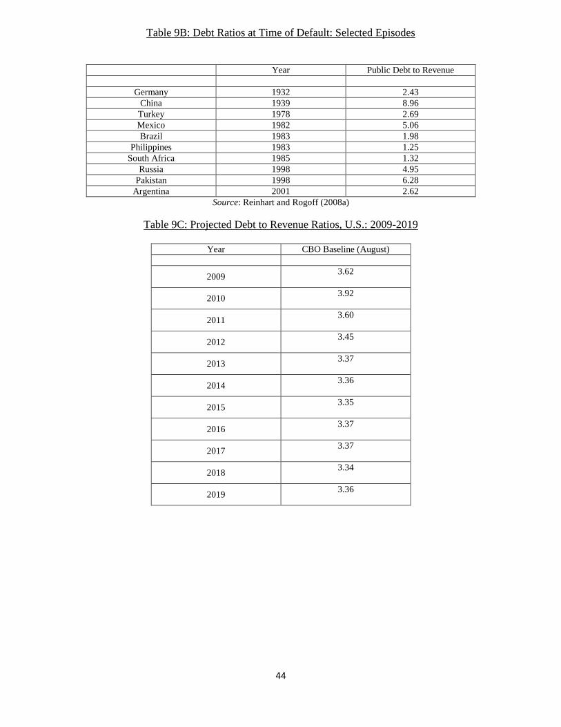
44

Table 9B: Debt Ratios at Time of Default: Selected Episodes

Year Public Debt to Revenue

Germany 1932 2.43

China 1939 8.96

Turkey 1978 2.69

Mexico 1982 5.06

Brazil 1983 1.98

Philippines 1983 1.25

South Africa 1985 1.32

Russia 1998 4.95

Pakistan 1998 6.28

Argentina 2001 2.62

Source: Reinhart and Rogoff (2008a)

Table 9C: Projected Debt to Revenue Ratios, U.S.: 2009-2019

Year CBO Baseline (August)

2009 3.62

2010 3.92

2011 3.60

2012 3.45

2013 3.37

2014 3.36

2015 3.35

2016 3.37

2017 3.37

2018 3.34

2019 3.36