The Decline of Activist Stabilization Policy:

Natural Rate Misperceptions, Learning, and Expectations

Athanasios OrphanidesBoard of Governors of the Federal Reserve System

andJohn C. Williams∗

Federal Reserve Bank of San Francisco

December 2003

Abstract

We develop an estimated model of the U.S. economy in which agents form expectationsby continually updating their beliefs regarding the behavior of the economy and mone-tary policy. We explore the effects of policymakers’ misperceptions of the natural rateof unemployment during the late 1960s and 1970s on the formation of expectations andmacroeconomic outcomes. We find that the combination of monetary policy directed attight stabilization of unemployment near its perceived natural rate and large real-time er-rors in estimates of the natural rate uprooted heretofore quiescent inflation expectationsand destabilized the economy. Had monetary policy reacted less aggressively to perceivedunemployment gaps, inflation expectations would have remained anchored and the stagfla-tion of the 1970s would have been avoided. Indeed, we find that less activist policies wouldhave been more effective at stabilizing both inflation and unemployment. We argue thatpolicymakers, learning from the experience of the 1970s, eschewed activist policies in fa-vor of policies that concentrated on the achievement of price stability, contributing to thesubsequent improvements in macroeconomic performance of the U.S. economy.

Keywords: Monetary policy, stagflation, rational expectations, learning.

JEL Classification System: E52

Correspondence: Orphanides: Federal Reserve Board, Washington, D.C. 20551, Tel.: (202) 452-2654,e-mail: Athanasios.Orphanides@frb.gov. Williams: Federal Reserve Bank of San Francisco, 101Market Street, San Francisco, CA 94105, Tel.: (415) 974-2240, e-mail: John.C.Williams@sf.frb.org.∗We would like to thank Alex Cukierman, Vitor Gaspar, Glenn Rudebusch, Robert Solow, andparticipants at presentations at Georgetown University, the Workshop on Expectations, Learning andMonetary Policy, Eltville, August 30–31, 2003, and the International Research Forum on MonetaryPolicy, Washington, D.C., November, 14–15, 2003, for useful comments and discussions on earlierdrafts. Kirk Moore provided excellent research assistance. The opinions expressed are those of theauthors and do not necessarily reflect views of the Board of Governors of the Federal Reserve Systemor the management of the Federal Reserve Bank of San Francisco.

1 Introduction

The “New Economics” of the 1960s prescribed activist policies aimed at achieving and main-taining full employment of economic resources. According to this view, active managementof aggregate demand would counteract any shortfalls or excesses relative to the economy’spotential and thus attain the holy grail of macroeconomic policy: sustained prosperity withprice stability. This faith in macroeconomic stabilization policy reflected the culmination ofmethodological advances in macroeconomic modeling, econometrics, and optimal control.1

The zeitgeist of the “New Economics” is nicely summarized by Walter Heller (1966):

The promise of modern economic policy, managed with an eye to maintain-ing prosperity, subduing inflation, and raising the quality of life, is indeed great.And although we have made no startling conceptual breakthroughs in economicsin recent years, we have, more effectively than ever before, harnessed the ex-isting economics—the economics that has been taught in the nation’s collegeclassrooms for some twenty years—to the purposes of prosperity, stability, andgrowth. (page 116, emphasis in original.)

The enviable performance of the U.S. economy in the first half of the 1960s appeared

to validate the claims of Heller, but this success proved to be fleeting. In the second half

of the 1960s, prosperity was purchased at the cost of rising inflation, as seen in Figure 1.

Worse, the prosperity of the 1960s was soon overshadowed by the stagflation–high inflation

accompanied by high unemployment–in the 1970s.

In this paper, we reexamine the sources of stagflation in the 1970s, and argue that the

combination of monetary policy directed at tight stabilization of the unemployment rate

near its perceived natural rate and severe underestimation of the natural rate, rather than

adverse supply shocks, explains much of the woeful performance of the U.S. economy in the

1970s. With hindsight, it is clear that policymakers in the 1960s and much of the 1970s

were far too optimistic of how low the unemployment rate could go before igniting inflation

pressures. Given the activist bent of policymakers influenced by the “New Economics,” these

natural rate misperceptions contributed to an extended period of policy being excessively

stimulative, resulting in rising inflation.2

1See Heller (1966), Tobin (1966, 1972) and Okun (1970) for discussions of the ideas associated with the“New Economics” of the 1960s. Application of control methods for macroeconomic stabilization had beendiscussed at least as early as Lerner (1944) and formalized by Phillips (1954). Friedman’s (1947) review ofLerner (1944) offers an early critique of the application of these methods for macroeconomic stabilization.

2See Orphanides (2002, 2003a,b, forthcoming), Orphanides and Williams (2002), Bullard and Eusepi(2003), Collard and Dellas (2003), and Cukierman and Lippi (2003).

1

A key element in our analysis is the endogenous evolution of expectations formation

in response to the tumultuous economic developments of the late 1960s and 1970s. We

develop an estimated model of the U.S. economy in which private agents have imperfect

knowledge of the true structure of the economy and policy. In the model, agents are assumed

to continuously update their beliefs about the reduced-form structure of the economy and

monetary policy. As discussed in Orphanides and Williams (2003, forthcoming), this process

of perpetual learning propagates the direct effects of policy errors onto inflation expectations

and back on the economy.

According to our model, the combination of stimulative monetary policy and rising in-

flation during the late 1960s and 1970s contributed to private agent confusion regarding the

Federal Reserve’s objectives and the behavior of inflation. Although inflation expectations

were initially well-anchored owing to the period of price stability in the 1950s and early

1960s, this advantage was squandered during the late 1960s as policy errors and the result-

ing rise in inflation caused inflation expectations to drift upward.3 By the time that the

supply shocks of the 1970s hit, inflation expectations were already unmoored, exacerbating

the response to the shocks and contributing to stagflation. It is worth noting that our results

do not rely on policy being inherently destabilizing in the pre-1979 period, as emphasized

by Clarida, Gali, and Gertler (2000). In fact, the feedback rule that we estimate for the

pre-1979 period based on real-time data features a greater than one-for-one response of

nominal rates to inflation. What is crucial for our results is that policy responded strongly

to perceived unemployment rate gaps during that period as indicated by our estimated

policy feedback rule.

We find that had monetary policy not reacted as aggressively to perceived unemployment

gaps as it did, inflation expectations would have remained anchored and the stagflation

of the 1970s would have been avoided, despite the dramatic increases in oil prices and

the productivity slowdown during that period. Importantly, according to our model, less

activist policies would have done a better job of stabilizing both inflation and unemployment

in the 1970s. This is a lesson that policymakers themselves appeared to recognize by end3The favorable environment of inflation expectations in the early 1960s can be largely attributed to

the greater emphasis on price stability relative to economic stabilization before the decade of the 1960s.See Romer and Romer (2002) and Orphanides (2003c) for discussions highlighting some underappreciatedpositive aspects of the policy environment during this period.

2

of the 1970s. At that time, with inflation seemingly spiraling out of control, monetary

policymakers in the United States changed course, eschewing the fine-tuning of the “New

Economics” and concentrating instead on the goal of price stability. Indeed, in 1978, before

he became Chairman of the Federal Reserve Board of Governors, Paul Volcker alluded to

the nature of the required change:4

Wider recognition of the limits on the ability of demand management to keepthe economy at a steady full employment path, especially when expectations arehypersensitive to the threat of more inflation, provides a more realistic startingpoint for policy formulation. (1978 p. 61.)

Following the costly disinflation of the early 1980s, less activist monetary policy, as evi-

denced by a reduced policy responsiveness to the perceived unemployment gap, contributed

to a new era of relatively stable inflation and unemployment. Our model helps explain

this evolution in the understanding of the role of monetary policy and the critical nature

of maintaining well anchored inflation expectations as a means for ensuring long-term eco-

nomic stability.

2 Natural Rate Misperceptions and Policy Activism

The success of activist stabilization policy rests on the assumption that the natural rate is

a useful policy target. Under that assumption, adjusting aggregate demand relative to the

economy’s natural rate becomes the focus of short-term stabilization policy. Many of the

policy errors associated with the Great Inflation of the late 1960s and 1970s can be traced

to the pursuit of too low of a target of the natural rate of unemployment.

Figure 2 plots the rate of unemployment in the United States since the end of 1965

(the beginning of the Great Inflation) and two measures of the natural rate, a real-time

measure, that is, perceptions as of the time shown, and a retrospective measure, that is,

a current estimate. We take the current Congressional Budget Office (CBO) (2001, 2002)

estimates of the natural rate of unemployment as truth. We construct a real-time series

for the natural rate guided by written documents that offer glimpses of the thinking of

policymakers of the 1960s and 1970s. During the 1960s, four percent was widely accepted4During the early stages of the disinflationary policy pursued following the 1979 policy change, Chairman

Volcker often stressed the importance of policies anchoring inflation expectations.

3

as a reasonable working definition of the full employment rate of unemployment.5 Although

we do not have precise information for the evolution of real-time perceptions of the natural

rate of unemployment in the early 1970s, we do know that many estimates rose during that

period, as reflected in various policy-related studies.6 Correspondingly, we posit that per-

ceptions of the natural rate rose to around 4.5 percent in 1970 from the 4 percent estimates

that prevailed earlier.7 Published accounts of Federal Reserve Board model exercises and

estimates by the Council of Economic Advisers reported in the Economic Report of the

President indicate that natural rate estimates continued to rise during the 1970s. From the

late 1970s to the present, the CBO has regularly reported, explicitly or implicitly, its esti-

mates of the natural rate in its publications regarding the economic and budget outlook,

and for those years we use the contemporaneous values for our real-time estimates from

these CBO publications.8

Comparison of the real-time perceptions likely held by policymakers at the time and

our best current measures of the natural rate, then, provide a summary indicator of the

potential policy errors that may be committed when an activist approach to stabilization

policy is pursued. The top panel of Figure 3 shows our real-time and retrospective estimates

of the natural rate of unemployment. The bottom panel of the figure plots the implied

natural rate misperceptions—measured as the “true” value minus the real-time estimate—

from 1965 through 2003. As seen in the figure, natural rate misperceptions have tended

to be highly persistent. The first-order serial correlation of this series over this sample is

0.98. Interestingly, the average magnitude of real-time misperceptions has declined over the

past several decades. This appearance of diminishing errors may be overstated, however,

because these calculations of “errors” implicitly assume that the current CBO method of5Recollections of key policymakers of that period, including Walter Heller, Arthur Okun and Herbert

Stein, who served as members and chairs of the Council of Economic Advisers in the 1960s and early 1970s,as well as Federal Reserve Chairman Arthur Burns serve as evidence of the wide acceptance of that estimate.See Burns (1979), Heller (1966), Okun (1962, 1970), and Stein (1984, 1996).

6See, for example, the discussion in Hall (1970) and Perry (1970).7As a robustness check, we considered alternative paths for the real-time estimates in the model-based

simulation exercises reported below. The precise dating of the evolution of perceptions regarding the rise ofthe natural rate from 4 percent in the late 1960s to 5 percent in the late 1970s does not materially influenceour simulations, as both the pattern and size of the resulting misperceptions remain broadly similar undersuch alternatives, given that the retrospective estimates for this period, at about 6 percent, are always higherby a considerable margin.

8The real-time and retrospective natural rate estimates of the most recent five years are identical, reflect-ing the fact that the CBO’s estimates are unchanged over that period.

4

estimating the natural rate is correctly specified. The real-time and retrospective estimates

in the latter part of the sample are constructed using the same method (based on a Kalman

filter), while the “misperceptions” in the earlier part of the sample also reflect differences

in methodology. If the current methodology used by the CBO proves to be inadequate,

then the difference between real-time estimates and retrospective estimates in the 1980s

and 1990s may widen in the future.9

Examples from the 1970s illustrate the problem associated with adopting an activist

approach to stabilization policy when one may be mistaken as to the size or even the sign

of the unemployment (or output) gap in real time.10 Consider the policy error of the early

1970s. With unemployment rising during and after the recession that started at the end of

1969, and in light of available estimates of the natural rate of unemployment, policymakers

could have reasonably held the view that the economy was operating with considerable

slack. The activist policy prescription at the time was clear cut: pursue additional monetary

expansion to bring the unemployment rate down. Moreover, the existing slack should have

led to some welcome disinflation despite the additional stimulus. Indeed, such a policy was

pursued at the time. But, based on the retrospective estimates of the natural rate, it is

now clear that that policy prescription represented a large error. The economic expansion

pursued in 1971-73 pushed aggregate demand far above the economy’s potential, as this is

currently understood, fueling an increase in inflation. A similar error occurred after the

1975 recession, contributing to a further rise in inflation.

3 A Simple Estimated Model of the U.S. Economy

We examine the interaction of natural rate misperceptions, learning, and expectations for

alternative monetary policy rules using a simple quarterly forward-looking model we de-

veloped in Orphanides and Williams (2002). The specification of the model is unchanged

from that paper; however, we have reestimated the structural equations using the retrospec-

tive and real-time estimates of the natural rate of unemployment reported in the preceding

section and, for simplicity, we have imposed a constant implicit natural rate of interest.9See Orphanides and Williams (2002) for a detailed discussion of the sensitivity of measures of natural

rate misperceptions to the assumption of the correct estimation method.10See Orphanides and van Norden (2002) and Orphanides and Williams (2002) for summary documentation

of the magnitude of the problem of real-time measurement of the natural rates of output and unemployment,respectively.

5

3.1 The Structural Model

The model consists of the following two structural equations:

πt = φππet+1 + (1 − φπ)πt−1 + απ(ue

t − u∗t ) + eπ,t, eπ ∼ iid(0, σ2

eπ), (1)

ut = φuuet+1+χ1ut−1+χ2ut−2+(1−φu−χ1−χ2)u∗

t +αu (rat−1−r∗)+eu,t, eu ∼ iid(0, σ2

eu),

(2)

where π denotes the annualized log difference of the GNP or GDP price deflator, u denotes

the unemployment rate, u∗ denotes the true natural rate of unemployment, ra denotes

the real interest rate based on the one-year Treasury bill, and r∗ the natural real rate of

interest. This model combines forward-looking elements of the New Synthesis model studied

by Goodfriend and King (1997), Rotemberg and Woodford (1999), Clarida, Gali and Gertler

(1999), and McCallum and Nelson (1999), and others, with the intrinsic inflation and inertia

in the level of economic activity featured in Fuhrer and Moore (1995), Brayton et al (1997),

Smets (2000), Fuhrer and Rudebusch (forthcoming), and others.

The “Phillips curve” in this model (equation 1) relates inflation (measured as the an-

nualized percent change in the GNP or GDP price index, depending on the period) during

quarter t to lagged inflation, expected future inflation, and expectations of the unemploy-

ment gap during the quarter, using the retrospective estimates of the natural rate discussed

below. The estimated parameter φπ measures the importance of expected inflation on the

determination of inflation. The unemployment equation (equation 2) relates the unem-

ployment gap during quarter t to the expected future unemployment gap, two lags of the

unemployment gap, and the lagged real interest rate gap. Here two elements importantly

reflect forward-looking behavior. The first element is the estimated parameter φu, which

measures the importance of expected unemployment, and the second is the duration of the

real interest rate, which serves as a summary of the influence of interest rates of various

maturities on economic activity. Because data on long-run inflation expectations are not

available, we limit the duration of the real rate to one year.

One difficulty in estimating this model is that expected inflation and unemployment

are not directly observed. Instrumental variable and full-information maximum likelihood

methods impose the restriction that the behavior of monetary policy and the formation

of expectations be constant over time, neither of which appears tenable over our sample

6

period (1969–2002). Instead, as in Orphanides and Williams (2002), we follow the approach

suggested by Roberts (1997), and also employed by Rudebusch (2002), and use the Survey

of Professional Forecasters as the source for proxies for expectations. Specifically, we use

the median values of the forecasts provided in the Survey and posit that the relevant expec-

tations are those formed in the previous quarter; that is, we assume that the expectations

determining πt and ut are those collected in quarter t − 1. Finally, to match the inflation

and unemployment data as best as possible with these forecasts, we use first announced es-

timates of these series.11,12 Our primary sources for our data are the Real-Time Dataset for

Macroeconomists and the Survey of Professional Forecasters, both currently maintained by

the Federal Reserve Bank of Philadelphia (Zarnowitz and Braun (1993), Croushore (1993)

and Croushore and Stark (2001)). Using ordinary least squares, we obtain the following

estimates for our model between 1969:1 and 2002:2:13

πt = 0.529(0.086)

πet+1 + 0.471

(−−)

πt−1 − 0.304(0.093)

(uet − u∗

t ) + eπ,t, (3)

SER = 1.38, DW = 2.09,

ut = 0.221(0.080)

uet+1 + 1.262

(0.104)

ut−1 − 0.529(0.068)

ut−2 + 0.045(0.022)

u∗t + 0.033

(0.013)

(rat−1 − r∗) + eu,t, (4)

SER = 0.29, DW = 2.08,

The numbers in parentheses are the estimated standard errors of the corresponding regres-

sion coefficients. The estimated unemployment equation also includes a constant term that

provides an estimate of the natural real interest rate plus the average premium of the one-

year Treasury bill rate we use for estimation over the federal funds rate, which corresponds

to the natural rate of interest estimates we use in the model. If this premium equals the

average difference between the one-year rate and the federal funds rate during this sample,

then the estimation suggests that the natural rate of interest in this sample is 3.2 percent.11This implies that the relevant expectations surprises influencing current outcomes are those perceived on

the basis of first announced data and not those defined retrospectively on the basis of subsequent revisions.We adopt this simplification for its parsimony, recognizing that subsequent revisions of historical data mayat times affect economic decisions in a more complicated manner.

12This is also common in forecast evaluation experiments; for example, Romer and Romer (2000) usefirst-announced outcomes in their evaluation of Federal Reserve Board Greenbook forecasts.

13The starting point of this sample reflects the availability of the Survey of Professional Forecasters data.

7

To complete our model for simulations, we impose the expectations theory of the term

structure whereby the one-year rate equals the expected average of the federal funds rate

over four quarters.

3.2 Historical Monetary Policy

In addition to the equations for inflation and the unemployment rate, we estimate a mone-

tary policy rule according to which the federal funds rate is determined by the lagged funds

rate, the forecast of inflation over the next year (defined to be the four-quarter change from

t − 1 to t + 3 where t denotes the period for which the funds rate is set), the forecasted

change in the unemployment rate over the next year, and the unemployment gap (the un-

employment rate less the real-time estimate of the natural rate) forecasted to occur in three

quarters:

it = θiit−1 + (1− θi)(r∗ + π∗) + θπ(πet+3 − π∗) + θu(ue

t+3 − u∗t ) + θ∆u(ue

t+3 − ut−1) + εi,t (5)

For both estimation and simulation purposes, we assume that the central bank responds

to the private sector forecasts of inflation and the unemployment rate in setting policy. As

discussed in Orphanides (2003c) and Orphanides and Williams (2002), this specification

nests both a version of the classic Taylor rule (Taylor, 1993), which excludes the change in

unemployment and lagged interest rate terms (that is sets θi = θ∆u = 0), as well as rules

robust to natural rate misperceptions (the limiting case with θi = 1 and θu = 0)

To allow the rule to capture the reduction of activism in Federal Reserve policy following

the summer of 1979, we allow for a break in the policy rule at that time. Other things

equal, a reduction in activism should be reflected in this rule by a reduction in the policy

responsiveness to the perceived gap in the forecast of unemployment from its natural rate,

θu. To examine this effect in a parsimonious manner, we follow the suggestion in Orphanides

(forthcoming) and focus on a specification that allows for a break in the θu parameter,

keeping remaining parameters of the policy reaction functions fixed.14 Allowing for this

break, our estimated policy rule is given by:14A stability test rejects the constancy of all parameters over the two subsamples. However, once we allow

for the break in θu, the stability of individual remaining parameters over the two subsamples cannot berejected. As a robustness check for our model, we also examined simulations based on a specification of thepolicy rule that allows breaks in two parameters, θu and θπ. In that specification, the point estimates ofboth θπ and θu are slightly lower in the first subsample, but the difference is small and does not qualitativelyinfluence our simulation results.

8

it = 0.750(0.044)

it−1 + 0.250(−−)

(r∗ + π∗) + 0.779(0.130)

(πet+3 − π∗) − 0.673

(0.210)

(uet+3 − ut−1)+

( − 1.131(0.197)

+ 0.561(0.158)

D) (uet+3 − u∗

t ) + εi,t, (6)

SER = 1.02, DW = 1.90,

where D is a dummy variable equaling zero before 1979:3 and one thereafter. Conditional

on a value for the natural rate of interest, r∗, estimation of this policy rule also provides

an estimate of the implicit inflation target, π∗. Assuming r∗ = 3.2 percent, as suggested by

the estimation of equation 2, yields an estimate of 2.7 percent for π∗ with a standard error

equal to 0.15 percent.

As can be seen, and consistent with the narrative evidence, the estimated policy reaction

function points to a substantial reduction in policy activism following the summer of 1979

compared to the earlier period. We note that this policy rule satisfies the standard stability

condition in models with adaptive or rational expectations that the long-run response of

the nominal interest rate to a change in the inflation rate exceeds unity. We do not find

evidence that policy was inherently destabilizing in the pre-1979 sample, but instead only

that it was more activist. This contrasts with the well-known findings reported by Clarida,

Gali and Gertler (2000), based on a similar specification, but employing the output gap

(instead of the unemployment gap) and relying on instrumental variables analysis with

ex post data (instead of real-time data and forecasts). They suggested that the response

of policy to inflation was unstable in the pre-1979 period. However, as documented by

Orphanides (forthcoming), their findings are overturned when information actually available

to policymakers in real time is used to estimate the policy rule that they specify. Even when

we allow for breaks in the policy response to both expected inflation and to the perceived

unemployment gap in our rule, which, as noted earlier, suggests that the coefficient on the

inflation forecast is a bit lower in the pre-1979 sample, we find that the estimation provides

no evidence supporting the hypothesis of policy instability.

9

4 Expectations Formation

Following Orphanides and Williams (2003, forthcoming), we assume that agents reestimate

their forecasting models each period using a constant gain algorithm that places more weight

on recent observations.15 Given the structure of the model, agents need to forecast inflation,

the unemployment rate, and the federal funds rate for up to four quarters in the future. As

noted above, we assume the policymaker uses private agents’ forecasts in setting policy.

4.1 Least Squares Learning with Finite Memory

Under perfect knowledge with no shocks to the natural rate of unemployment, the pre-

dictable components of inflation, the unemployment rate, and the funds rate each depend

on a constant, one lag each of the inflation and the ex post real funds rate (the difference

between the nominal funds rate and the inflation rate), and two lags of the unemployment

rate. We assume that agents estimate forecasting equations for the three variables using a

restricted VAR of this form. They then construct multi-period forecasts from the estimated

VAR. To fix notation, let Yt denote the 1×3 vector consisting of the inflation rate, the unem-

ployment rate, and the federal funds rate, each measured at time t: Yt = (πt, ut, it); let Xt

be the 5×1 vector of regressors in the forecast model: Xt = (1, πt−1, ut−1, ut−2, it−1−πt−1);

let ct be the 5 × 3 vector of coefficients of the forecasting model.

Using data through period t, the least squares regression parameters for the forecasting

model can be written in recursive form:

ct = ct−1 + κtR−1t Xt(Yt − X ′

tct−1), (7)

Rt = Rt−1 + κt(XtX′t − Rt−1), (8)

where κt is the gain.

Under the assumption of least squares learning with infinite memory, κt = 1/t, so as t

increases, κt converges to zero. As a result, as the data accumulate this mechanism converges

to the correct expectations functions and the economy converges to the perfect knowledge

benchmark solution. As noted above, to formalize perpetual learning—as would be implied15See also Sargent (1999), Cogley and Sargent (2001), Evans and Honkapohja (2001), and Gaspar and

Smets (2002) for related treatments of learning. A separate strand of the literature has focused on theproblem of estimating the implicit inflation target of the central bank, assuming that other parameters areknown. See e.g. Bomfim et al (1997), Erceg and Levin (2003), Kozicki and Tinsley (2003), and Rudebuschand Wu (2003).

10

by the presence of structural changes such as shifts in the natural rate of unemployment—

we replace the decreasing gain in the infinite memory recursion with a small constant gain,

κ > 0.16

With imperfect knowledge, expectations are based on the perceived law of motion of

the inflation process, governed by the perpetual learning algorithm described above. The

model under imperfect knowledge consists of the structural equations for inflation, the

output gap, the federal funds rate (the monetary policy rule), and the forecasts generated

from the forecasting model.

We should emphasize that in the limit of perfect knowledge (that is, as κ → 0) and

assuming a constant natural rate of unemployment, the expectations function above con-

verges to rational expectations, and the stochastic coefficients for the forecasting model

converge to those implied by the structural model equations under rational expectations.

As explained in Orphanides and Williams (forthcoming), this modeling approach accom-

modates the Lucas critique in the sense that expectations formation is endogenous and

adjusts to changes in policy or structure; and, although expectations are “imperfectly” ra-

tional, in that agents are required to estimate the reduced form processes needed to form

expectations, the resulting expectations are close to being efficient.

4.2 Calibrating the Learning Rate

A key parameter for the constant-gain-learning algorithm is the updating rate κ. To cali-

brate this parameter we examined how well different values of κ fit either the expectations

data from the Survey of Professional Forecasters, or, based on our model, the actual data

on inflation and unemployment.

To examine the fit of the Survey of Professional Forecasters (SPF), we generated a time

series of forecasts using a recursively estimated VAR for the inflation rate, the unemploy-

ment rate, and the federal funds rate. In each quarter we reestimated the model using all

historical data available during that quarter (generally from 1948 through the most recent

observation). We allowed for discounting of past observations by using geometrically declin-

ing weights. We found that discounting past data at about 1 percent per quarter yielded16In terms of forecasting performance, the “optimal” choice of κ depends on the relative variances of the

transitory and permanent shocks, as in the relationship between the Kalman gain and the signal-to-noiseratio in the case of the Kalman filter.

11

forecasts closest on average to the SPF over 1968–2002.17 This corresponds to an updating

gain of about 2 percent per quarter during the 1970s and 1-1/2 percent per quarter in the

1990s.

To examine the degree of discounting that best fits the historical data on inflation and

unemployment, given our structural model and learning process, we simulated the model

from 1966 forward for alternative values of κ and examined the mean squared deviations of

the simulated path from the actual paths of inflation and unemployment. (Details on simu-

lation of the model and setting of initial conditions are provided below.) These simulations

suggested that our model with values of κ between 0.01 and 0.04 matched the data better

than when κ was set at lower or higher values.

In light of these results, in the following we use κ = 0.02 as a baseline value. As a

robustness check, we also examined the sensitivity of our model to lower and higher values.

5 The Interaction of Learning, Misperceptions, and Policy

We examine a set of alternative counterfactual simulations to investigate the role of learning,

natural rate misperceptions, and policy for understanding the behavior of inflation and

unemployment and the evolution of policy. We start our simulations at the beginning of

1966, which corresponds to what many observers consider to be the beginning of the Great

Inflation in the United States.

5.1 Initial Conditions

The states of the model economy with learning are: the current value and one lag each of the

inflation rate and the federal funds rate, the current value and two lags of the unemployment

rate, the true natural rate of unemployment, the real-time estimate of the natural rate, the

shocks to the structural equations, and the matrices C and R for the forecasting model. We

initialize the C and R matrices using estimates of the forecasting model by ordinary least

squares on data from 1948 through 1965.

Based on our calibration of the learning rate using survey data, we set κ = 0.02 and

compute the implied forecasts of inflation, the unemployment rate, and the federal funds17This finding is also in line with the discounting reported by Sheridan (2003) as best for explaining the

inflation expectations data reported in the Livingston Survey.

12

rate over 1966:1 – 2003:2. Using these forecasts as data, we then compute tracking residuals

for all model equations so that the model identically matches the data over the full sample.

5.2 The Role of Natural Rate Misperceptions

Our first experiment is a simulation in which policy follows the estimated policy rule (in-

cluding residuals), but the policymaker is assumed to observe the true value of the natural

rate of unemployment in real time. That is, there are no natural rate misperceptions. Note

that because the policy rule matches history under the assumption that the policy was

based on the real-time estimates of the natural rate, the simulation boils down to adding

innovations to the policy rule equal to the coefficient on the unemployment gap multiplied

by the real-time misperceptions shown in Figure 3.

Absent natural rate misperceptions, inflation would have been relatively stable in the

1970s according to the model. Figure 4 shows the historical paths (the thick lines) and

the simulated paths of the rates of inflation (four-quarter change in the price level) and

unemployment. In contrast to the historical experience when inflation reached into double

digits, the inflation rate with no natural rate misperceptions remains in a relatively narrow

range of about 2 percent to 4 percent during the 1970s. The stability in inflation is achieved

through a tighter path for policy starting in 1966 that drives the unemployment rate above

its historical path. This effective stabilization of inflation avoids the rise in unemployment

associated with the Volcker disinflation occurring at the end of the decade and into the

early 1980s.

The policy without natural rate misperceptions also avoids the damaging shift in the

perceived law of motion of inflation evident in the historical data. Absent the rise in inflation

in the late 1960s and 1970s, the expected level of inflation also remains subdued. In addition,

the perceived persistence in inflation remains moderate. The thick solid line in Figure 5

shows the estimated sum of coefficients on lagged inflation in the forecasting equation for

inflation that incorporates learning, as described above. This statistic usefully summarizes

agents’ perceptions of the persistence in inflation. Based on the historical data, the perceived

persistence in inflation rises to about 0.9 by 1975.18 In contrast, under the same policy,18This rise in perceived inflation persistence in our model is a manifestation of the real-world accumulation

of evidence against the hypothesis of a long-run tradeoff between unemployment and inflation and in favorof the “accelerationist” view during the 1970s.

13

but absent natural rate misperceptions, the perceived persistence in inflation would have

remained moderate throughout the 1960s and 1970s. In this simulation, the trend rise in

inflation associated with the “Great Inflation” is avoided and inflation expectations remain

well anchored.

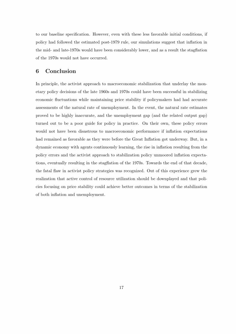
5.3 The Role of Learning

Even in the presence of policy errors driven by misperceptions of the natural rate of un-

employment, economic outcomes during the Great Inflation could have been much less

unfavorable if expectations had remained well anchored and governed by the forecasting

processes in place before. With regard to the persistence of inflation, had the policy errors

of the late 1960s and 1970s not resulted in its steep increase, inflation would have been con-

tained much more easily and price stability restored at a lower cost. To illustrate the role

of learning in this case, Figure 6 presents a counterfactual experiment where the historical

policy rule is followed, and policy continues to make the errors associated with natural rate

misperceptions, but the process governing the formation of expectations is unaffected by

the resulting adverse outcomes and continues to be governed by the reduced form VAR in

place at the beginning of the simulation, in 1966. Thus, in this simulation, expectations

of inflation remain by design well anchored through time. As can be seen, despite the

policy errors due to the natural rate misperceptions, in the absence of learning, that is if

the favorable expectations mechanism in place before the Great Inflation could have been

maintained, economic outcomes would have been significantly better.

5.4 The Role of Policy Activism

The simulations above suggest that under some conditions the activist policy pursued during

the Great Inflation could have been successful. In particular, if policymakers could have

avoided misperceptions in the natural rate or, if expectations could have remained favorable

even in the face of the policy errors caused by the combination of policy activism and

natural rate misperceptions, the stagflation of the 1970s would not have occurred. But, of

course, neither of these conditions could be taken for granted as the basis for policy design,

and the possibility that they might fail, as they did during the Great Inflation, limits the

scope for activist stabilization policy. An insufficient understanding of these limits and of

14

the long-term damage to expectations formation resulting from activist policy errors likely

contributed to the policy failure of the 1970s.

A natural question is whether a less activist approach, such as the one adopted following

the policy change in 1979, would have represented better policy during the Great Inflation as

well. To examine the role of policy activism, our third set of experiments examines what the

historical outcomes could have been in the presence of learning and of the observed natural

rate given by our real-time estimates if policy were driven by a less activist approach than

the one observed.19 Figures 7 and 8 summarize the results from two such experiments.

In one, policy does not respond to the unemployment gap at all, and in the other, policy

follows the estimated post-1979 reaction function.

If policymakers had followed either of these policies starting in 1966, the rise in inflation

in the 1970s would have been less pronounced and the unemployment rate would have been

lower on average than it actually was. The finding that both inflation and unemployment

would have been lower in the 1970s if the Fed had followed the estimated post-1979 re-

action function during the late 1960s and 1970s, or if the Fed had not responded to the

unemployment (or output) gap, differs from the results of Judd and Rudebusch (1998) and

Orphanides (2003b), respectively, who find that such policies would have implied lower in-

flation, but at the cost of lower output during the 1970s (implying a higher unemployment

rate). These analyses were based on the assumption of backward-looking accelerationist

models that implicitly treat inflation expectations as invariant to monetary policy. Our

results illustrate the importance of endogenous formation of expectations in affecting the

tradeoffs available to policymakers in designing monetary policies.

Importantly, as can be seen in Figure 8, under either policy, and even with the perpetual

learning process governing the formation of expectations, the natural rate misperceptions of

the 1960s and 1970s would not have been sufficient to destabilize the inflation expectations

process. By maintaining well-anchored inflation expectations throughout the 1970s, these

policies would have avoided the stagflationary outcomes of the decade.19This experiment is a first step towards investigating the design of efficient monetary policy in our

estimated model, accounting for the role of perpetual learning and its influence on the inflation expectationsprocess. An active literature over the past several years has been exploring issues related to efficient policydesign in the presence of uncertainty regarding models, data, and natural rates. See e.g. Levin et al (1999,2003), Orphanides (2003a), Orphanides et al (2000), Orphanides and Williams (2002), Rudebusch (2001,2002), and references therein.

15

Indeed, the realization of the role of the policy mistakes of the 1970s in destabilizing

inflation expectations was a key reason leading to the policy change in 1979. As Stephen

Axilrod summarized:20

Not all exogenous forces are purely exogenous. Rising inflationary expectationsin the late 1970s were in part the product of earlier monetary policies (as well asother events) as these policies affected attitudes toward the future, ... but onceembedded the expectations were exogenous to and influenced current policies—as in October 1979. (1985, p. 14.)

5.5 Robustness

As a robustness check for our key results regarding the wisdom of reduced policy activism, we

also examined counterfactual simulations under alternative assumptions regarding learning

and the formation of expectations. We concentrated our attention on the robustness of

the finding that if policy during the Great Inflation had followed the less activist approach

adopted after 1979, inflation expectations would have remained well behaved during the

1970s and the stagflation experienced during that decade would have been avoided.

We considered the sensitivity of our results to the updating parameter κ by comparing

counterfactual simulations for three different values of κ = 0.01, 0.02, 0.03 for the counter-

factual policy rule experiments. Qualitatively, the results are quite similar across the three

values of κ. In fact, the rise in the rate of inflation during the late 1970s appears less pro-

nounced both for the smaller and larger values of κ than in the baseline case of κ = 0.02. In

this sense, our baseline choice for κ is conservative in terms of the effects of the interaction

of learning and policy errors.

We also examined the sensitivity of our results for the choice of initial conditions govern-

ing the formation of expectations. Instead of the initial conditions estimated through the

end of 1965, we examined simulations with estimated initial conditions later in the sample.

We also considered as initial conditions the reduced-form coefficients corresponding to the

model-consistent solution of the model. In either case, these alternative initial conditions

are somewhat less favorable than the ones used in the simulations reported before. As a

result, inflation outcomes for the early 1970s are worse under these alternatives relative20Stephen Axilrod, a member of the Federal Reserve Board staff, served as the FOMC Economist at the

time of the 1979 policy change.

16

to our baseline specification. However, even with these less favorable initial conditions, if

policy had followed the estimated post-1979 rule, our simulations suggest that inflation in

the mid- and late-1970s would have been considerably lower, and as a result the stagflation

of the 1970s would not have occurred.

6 Conclusion

In principle, the activist approach to macroeconomic stabilization that underlay the mon-

etary policy decisions of the late 1960s and 1970s could have been successful in stabilizing

economic fluctuations while maintaining price stability if policymakers had had accurate

assessments of the natural rate of unemployment. In the event, the natural rate estimates

proved to be highly inaccurate, and the unemployment gap (and the related output gap)

turned out to be a poor guide for policy in practice. On their own, these policy errors

would not have been disastrous to macroeconomic performance if inflation expectations

had remained as favorable as they were before the Great Inflation got underway. But, in a

dynamic economy with agents continuously learning, the rise in inflation resulting from the

policy errors and the activist approach to stabilization policy unmoored inflation expecta-

tions, eventually resulting in the stagflation of the 1970s. Towards the end of that decade,

the fatal flaw in activist policy strategies was recognized. Out of this experience grew the

realization that active control of resource utilization should be downplayed and that poli-

cies focusing on price stability could achieve better outcomes in terms of the stabilization

of both inflation and unemployment.

17

References

Axilrod, Stephen (1985), “U.S. Monetary Policy in Recent Years: An Overview,” FederalReserve Bulletin, January, 14–24.

Bomfim, Antulio, Robert Tetlow, Peter von zur Muehlen, and John C. Williams (1997),”Expectations, Learning and the Cost of Disinflation,” in: Monetary Policy and theInflation Process, Basel, Switzerland: Bank for International Settlements.

Brayton, Flint; Mauskopf, Eileen; Reifschneider, David; Tinsley, Peter and Williams, John.“The Role of Expectations in the FRB/US Macroeconomic Model.” Federal ReserveBulletin, April 1997, 83(4), pp. 227–245.

Bullard, James and Stefano Eusepi (2003), “Did the Great Inflation Occur Despite Poli-cymaker Commitment to a Taylor Rule?” Federal Reserve Bank of St. Louis WorkingPaper 2003-012A, June.

Burns, Arthur (1979), The Anguish of Central Banking, The 1979 Per Jacobsson Lecture,Belgrade, Yugoslavia, September 30.

Clarida, Richard, Jordi Gali, and Mark Gertler (1999), “The Science of Monetary Policy,”Journal of Economic Literature, 37(4), 1661–1707, December.

Clarida, Richard, Jordi Gali, and Mark Gertler (2000), “Monetary Policy Rules and Macroe-conomic Stability: Evidence and Some Theory,” Quarterly Journal of Economics, 147–180, February.

Cogley, Timothy and Sargent, Thomas (2001), “Evolving Post-World War II U.S. InflationDynamics,” in NBER Macroeconomics Annual.

Collard, Fabrice and Harris Dellas (2003), “The Great Inflation of the 1970s,” mimeo,October.

Congressional Budget Office (2001), “CBO’s Method for Estimating Potential Output: AnUpdate,” Washington, DC: Government Printing Office (August).

Congressional Budget Office (2002), The Budget and Economic Outlook: An Update. Wash-ington DC: Government Printing Office (August).

Croushore, Dean (1993), “Introducing: The Survey of Professional Forecasters,” FederalReserve Bank of Philadelphia Business Review, November/December, 3–13.

Croushore, Dean and Tom Stark (2001), ”A Real-Time Data Set for Macroeconomists,”Journal of Econometrics 105, 111–130, November.

Cukierman, Alex and Francesco Lippi (2003), “Endogenous Monetary Poilicy with Unob-served Potential Output,” mimeo, December.

Erceg, Christopher J. and Andrew Levin (2003), “Imperfect Credibility and Inflation Per-sistence,” Journal of Monetary Economics. 50(4) 915-944, May.

Evans, George and Honkapohja, Seppo (2001), Learning and Expectations in Macroeco-nomics. Princeton: Princeton University Press.

Fuhrer, Jeffrey C. and George R. Moore (1995), “Inflation Persistence,” Quarterly Journalof Economics, 110(1), 127–59.

18

Fuhrer, Jeffrey C. and Glenn D. Rudebusch (forthcoming), “Estimating the Euler Equationfor Output,” Journal of Monetary Economics.

Friedman, Milton (1947), “Lerner on the Economics of Control,” Journal of Political Econ-omy, 55(5), October, 405–416.

Gaspar, Vitor and Smets, Frank (2002), “Monetary Policy, Price Stability and Output GapStabilisation,” International Finance, 5(2), Summer, 193–211.

Goodfriend, Marvin, and Robert King (1997), “The New Neoclassical Synthesis and theRole of Monetary Policy,” NBER Macroeconomics Annual, (12), 231–283.

Hall, Robert E. (1970), “Why Is the Unemployment Rate So High at Full Employment?”Brookings Papers on Economic Activity, 3, 369–402.

Heller, Walter W. (1966), New Dimensions of Political Economy, Cambridge, MA: HarvardUniversity.

Judd, John and Glenn Rudebusch (1998), “Taylor’s Rules and the Fed: 1970–1997,” FRBSFEconomic Review, 3, 3–16.

Kozicki, Sharon and Peter A. Tinsley (2003), “Permanent and Transitory Policy Shocks inMacro Models under Asymmetric Information,” Federal Reserve Bank of Kansas City,mimeo.

Lerner, Abba (1944), The Economics of Control, New York: Macmillan.

Levin, Andrew, Volker Wieland and John Williams (1999), “Robustness of Simple MonetaryPolicy Rules under Model Uncertainty,” in Monetary Policy Rules, John B. Taylor (ed.),Chicago: University of Chicago.

Levin, Andrew, Volker Wieland and John Williams (2003), “The Performance of Forecast-Based Policy Rules under Model Uncertainty,” American Economic Review, 93(3), 622–645, June.

McCallum, Bennett T. and Edward Nelson (1999), “Performance of Operational PolicyRules in an Estimated Semiclassical Structural Model.” in Monetary Policy Rules, JohnB. Taylor (ed.), Chicago: University of Chicago, 15–45.

Okun, Arthur (1962), “Potential Output: Its Measurement and Significance,” in Amer-ican Statistical Association 1962 Proceedings of the Business and Economic Section,Washington, D.C.: American Statistical Association.

Okun, Arthur (1970), The Political Economy of Prosperity, Brookings, Washington D.C.

Orphanides, Athanasios (2002), “Monetary Policy Rules and the Great Inflation,” AmericanEconomic Review, 92(2), 115-120, May.

Orphanides, Athanasios (2003a), “Monetary Policy Evaluation With Noisy Information,”Journal of Monetary Economics, 50(3), 605-631, April.

Orphanides, Athanasios (2003b), “The Quest for Prosperity Without Inflation,” Journal ofMonetary Economics, 50(3), 633-663, April.

Orphanides, Athanasios (2003c), “Historical Monetary Policy Analysis and the TaylorRule,” Journal of Monetary Economics, 50(5), 983-1022, July.

19

Orphanides, Athanasios (forthcoming), “Monetary Policy Rules, Macroeconomic Stabilityand Inflation: A View from the Trenches,” Journal of Money, Credit and Banking.

Orphanides, Athanasios, Richard Porter, David Reifschneider, Robert Tetlow and FredericoFinan (2000), “Errors in the Measurement of the Output Gap and the Design of Mon-etary Policy,” Journal of Economics and Business, 52(1/2), 117-141, January/April.

Orphanides, Athanasios and Simon van Norden (2002), “The Unreliability of Output GapEstimates in Real Time,” Review of Economics and Statistics, 84(4), 569–583, Novem-ber.

Orphanides, Athanasios and John C. Williams (2002), “Robust Monetary Policy Rules withUnknown Natural Rates”, Brookings Papers on Economic Activity, 2:2002, 63-118.

Orphanides, Athanasios and John C. Williams (2003), “Inflation scares and forecast-basedmonetary policy”, FRB San Francisco Working Paper, 2003-11 and FEDS 2003-41,August.

Orphanides, Athanasios and John C. Williams (forthcoming) “Imperfect Knowledge, In-flation Expectations and Monetary Policy,” in Inflation Targeting, Ben Bernanke andMichael Woodford (eds.), Chicago: University of Chicago Press.

Perry, George L. (1970), “Changing Labor Markets and Inflation,” Brookings Papers onEconomic Activity, 3, 411–448.

Phillips, A. W. (1954), “Stabilisation Policy in a Closed Economy,” Economic Journal,290–323, June.

Roberts, John M. (1997), “Is Inflation Sticky?” Journal of Monetary Economics, 39, 173–196.

Romer, Christina D. and David H. Romer (2000), “Federal Reserve Information and theBehavior of Interest Rates,” American Economic Review, 90(3), June, 429-457.

Romer, Christina and David Romer (2002), “A Rehabilitation of Monetary Policy in the1950s” American Economic Review, 92(2), May.

Rotemberg, Julio J. and Michael Woodford (1999), “Interest Rate Rules in an EstimatedSticky Price Model,” in Monetary Policy Rules, John B. Taylor (ed.), Chicago: Univer-sity of Chicago Press, 57–119.

Rudebusch, Glenn (2001), “Is the Fed Too Timid? Monetary Policy in an Uncertain World”Review of Economics and Statistics, 83(2), 203-17, May.

Rudebusch, Glenn (2002) “Assessing Nominal Income Rules for Monetary policy with Modeland Data Uncertainty,” Economic Journal, 112, 402-432, April.

Rudebusch, Glenn and Tao Wu (2003), “A Macro-Finance Model of the Term Structure,Monetary Policy, and the Economy” FRB/SF Working paper 2003-17, September.

Sargent, Thomas J. (1999), The Conquest of American Inflation, Princeton: PrincetonUniversity Press.

Sheridan, Niamh (2003), “Forming Inflation Expectations,” Johns Hopkins University,mimeo, April.

Smets, Frank (2000), “What Horizon for Price Stability,” European Central Bank WorkingPaper No 24.

20

Stein, Herbert (1984), Presidential Economics, New York: Simon and Schuster.

Stein, Herbert (1996), “A Successful Accident: Recollections and Speculations about theCEA,” 10(3), 3–21, Summer.

Taylor, John B. (1993), “Discretion versus Policy Rules in Practice,” Carnegie-RochesterConference Series on Public Policy, 39, December, 195–214.

Tobin, James (1966), National Economic Policy, New Haven: Yale University Press.

Tobin, James (1972), New Economics One Decade Older, Princeton: Princeton UniversityPress.

Volcker, Paul, A. (1978), The Rediscovery of the Business Cycle, New York: The Free Press.

Zarnowitz, Victor and Phillip A. Braun (1993), “Twenty-two Years of the NBER-ASAQuarterly Economic Outlook Surveys: Aspects and Comparisons of Forecasting Perfor-mance,” in Business Cycles, Indicators, and Forecasting, James H. Stock and Mark W.Watson (eds.), Chicago: University of Chicago Press, 11–84.

21

Figure 1

Inflation Rate

1965 1970 1975 1980 1985 1990 1995 2000 20050

2

4

6

8

10

12Percent

Notes: Inflation measured by the change of the output deflator (annual rate).

22

Figure 2

Unemployment and its Natural Rate

1965 1970 1975 1980 1985 1990 1995 2000 20053

4

5

6

7

8

9

10

11Percent

Actual unemployment rate Retrospective natural rate estimatesReal−time natural rate estimates

Notes: The retrospective natural rate reflects the current estimate of the NAIRU from theCongressional Budget Office. The real-time series is as described in the text.

23

Figure 3

The Natural Rate and Natural Rate Misperceptions

Estimates of the Natural Rate of Unemployment

1965 1970 1975 1980 1985 1990 1995 2000 20054

4.5

5

5.5

6

6.5Percent

Retrospective estimates (CBO)Real−time estimates

Real-Time Misperceptions of the Natural Rate

1965 1970 1975 1980 1985 1990 1995 2000 2005−2

−1.5

−1

−0.5

0

0.5

1Percentage point

24

Figure 4

Outcomes with No Natural Rate Misperceptions

Inflation Rate

1965 1970 1975 1980 1985 1990 1995 2000 2005−2

0

2

4

6

8

10

12Percent

Historical dataSimulated data absent U* misperceptions

Unemployment Rate

1965 1970 1975 1980 1985 1990 1995 2000 20053

4

5

6

7

8

9

10

11Percent

Historical dataSimulated data absent U* misperceptionsNatural rate of unemployment

Notes: The two panels show historical and simulated paths of the rates of inflation andunemployment. The thick solid lines show the historical data. The thin solid lines showthe simulated paths assuming that the monetary policymaker knows the true value of thenatural rate of unemployment in real time. The lightly-shaded thin solid line in the lowerpanel shows the assumed path for the natural rate of unemployment. Each simulation startsin the first quarter of 1966. 25

Figure 5

Evolution of Inflation Persistence in the Inflation Forecasting Equation

1965 1970 1975 1980 1985 1990 1995 2000 20050.3

0.4

0.5

0.6

0.7

0.8

0.9

1

Historical dataSimulated data absent U* misperceptions

Notes: The lines show the simulated paths of the sum of the coefficients on lagged inflationin agents’ inflation forecasting equations. The path shown by the thick line is based on thehistorical data. The thin line shows the simulated path in which the policymaker knowsthe true value of the natural rate of unemployment in real time. Each simulation starts inthe first quarter of 1966.

26

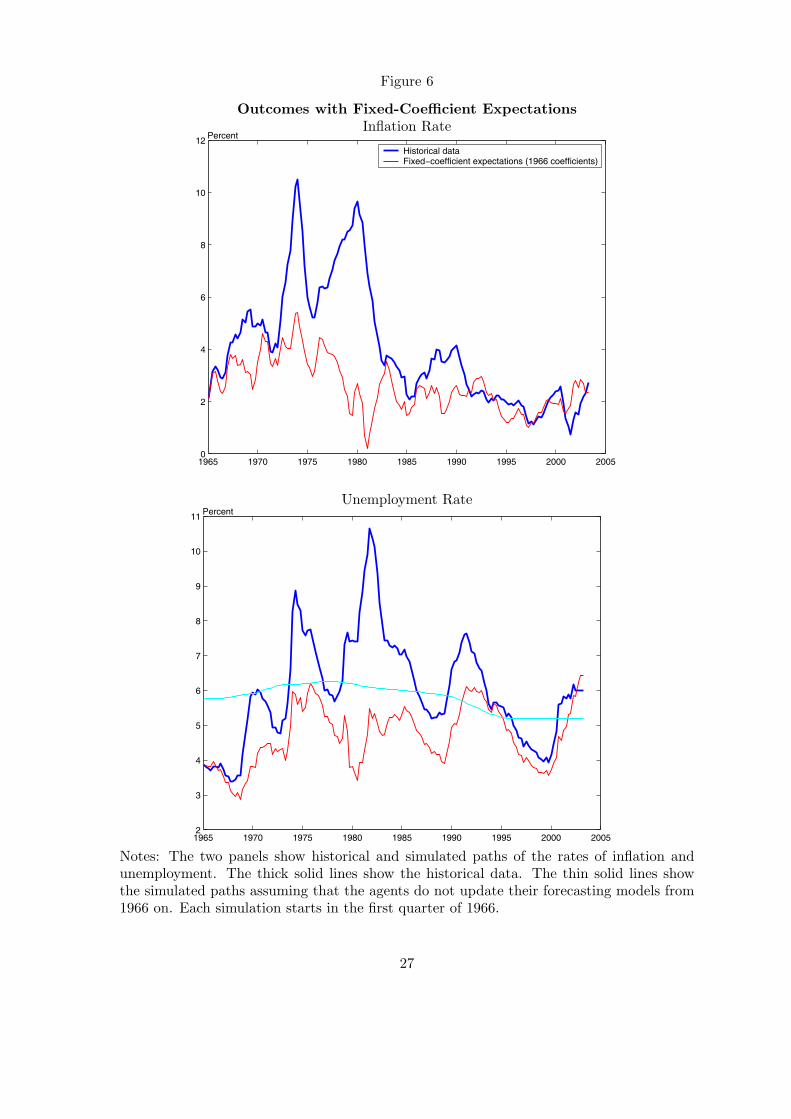
Figure 6

Outcomes with Fixed-Coefficient ExpectationsInflation Rate

1965 1970 1975 1980 1985 1990 1995 2000 20050

2

4

6

8

10

12Percent

Historical dataFixed−coefficient expectations (1966 coefficients)

Unemployment Rate

1965 1970 1975 1980 1985 1990 1995 2000 20052

3

4

5

6

7

8

9

10

11Percent

Notes: The two panels show historical and simulated paths of the rates of inflation andunemployment. The thick solid lines show the historical data. The thin solid lines showthe simulated paths assuming that the agents do not update their forecasting models from1966 on. Each simulation starts in the first quarter of 1966.

27

Figure 7

Outcomes with Alternative Policy Rules

Inflation Rate

1965 1970 1975 1980 1985 1990 1995 2000 20050

2

4

6

8

10

12Percent

Historical dataPost−79 policy ruleNo policy response to unemployment gap

Unemployment Rate

1965 1970 1975 1980 1985 1990 1995 2000 20052

3

4

5

6

7

8

9

10

11Percent

Historical dataPost−79 policy ruleNo policy response to unemployment gapNatural rate of unemployment

Notes: The two panels show historical and simulated paths of the rates of inflation andthe unemployment. The paths shown by the thick solid lines are based on the historicaldata. The thin solid lines show the simulated paths in which monetary policy follows thepost-1979 policy rule. The thick dashed lines show the simulated paths when policy doesnot respond to the unemployment gap. Each simulation starts in the first quarter of 1966.

28

Figure 8

Evolution of Inflation Persistence with Alternative Policy Rules

1965 1970 1975 1980 1985 1990 1995 2000 20050.3

0.4

0.5

0.6

0.7

0.8

0.9

1

Historical dataPost−79 policy ruleNo policy response to unemployment gap

Notes: The lines show the simulated paths of the sum of the coefficients on lagged inflationin agents’ inflation forecasting equations. The path shown by the thick solid line is basedon the historical data. The thin solid line shows the simulated path in which monetarypolicy follows the post-1979 policy rule. The thick dashed line shows the simulated pathwhen policy does not respond to the unemployment gap. Each simulation starts in the firstquarter of 1966.

29