Embed Size (px)
Citation preview

The DaMiRseq package - Data Mining for RNA-Seq data: normalization, feature selectionand classification
Mattia Chiesa 1 and Luca Piacentini 1
1Immunology and Functional Genomics Unit, Centro Cardiologico Monzino, IRCCS, Milan,Italy;
April 27, 2020
Abstract
RNA-Seq is increasingly the method of choice for researchers studying the transcriptome. Thestrategies to analyze such complex high-dimensional data rely on data mining and statisticallearning techniques. The DaMiRseq package offers a tidy pipeline that includes data miningprocedures for data handling and implementation of prediction learning methods to buildclassification models. The package accepts any kind of data presented as a table of rawcounts and allows the inclusion of variables that occur with the experimental setting. Aseries of functions enables data cleaning by filtering genomic features and samples, dataadjustment by identifying and removing the unwanted source of variation (i.e. batches andconfounding factors) and to select the best predictors for modeling. Finally, a “Stacking”ensemble learning technique is applied to build a robust classification model. Every stepincludes a checkpoint for assessing the effects of data management using diagnostic plots,such as clustering and heatmaps, RLE boxplots, MDS or correlation plots.
Package
DaMiRseq 2.0.0

The DaMiRseq package - Data Mining for RNA-Seq data: normalization, feature selection and classification
Contents
1 Citing DaMiRseq . . . . . . . . . . . . . . . . . . . . . . . . . . . 3
2 Introduction . . . . . . . . . . . . . . . . . . . . . . . . . . . . . . 4
3 Data Handling . . . . . . . . . . . . . . . . . . . . . . . . . . . . . 5
3.1 Input data . . . . . . . . . . . . . . . . . . . . . . . . . . . . 5
3.2 Import Data . . . . . . . . . . . . . . . . . . . . . . . . . . . 5
3.3 Preprocessing and Normalization . . . . . . . . . . . . . . . . . 63.3.1 Filtering by Expression . . . . . . . . . . . . . . . . . . . 73.3.2 Filtering By Coefficient of Variation (CV). . . . . . . . . . . . 73.3.3 Normalization . . . . . . . . . . . . . . . . . . . . . . . 83.3.4 Sample Filtering . . . . . . . . . . . . . . . . . . . . . . 8
3.4 Adjusting Data . . . . . . . . . . . . . . . . . . . . . . . . . . 93.4.1 Identification of Surrogate Variables . . . . . . . . . . . . . 93.4.2 Correlation between sv and known covariates . . . . . . . . . 103.4.3 Cleaning expression data . . . . . . . . . . . . . . . . . . 12
3.5 Exploring Data . . . . . . . . . . . . . . . . . . . . . . . . . . 13
3.6 Exporting output data . . . . . . . . . . . . . . . . . . . . . . . 24
4 Two specific supervised machine learning workflows . . . . . . 25
4.1 Finding a small set of informative, robust features . . . . . . . . . 264.1.1 Feature Selection . . . . . . . . . . . . . . . . . . . . . 264.1.2 Classification . . . . . . . . . . . . . . . . . . . . . . . 32
4.2 Building the optimal prediction model . . . . . . . . . . . . . . . 344.2.1 Training and testing inside the cross-validation . . . . . . . . . 354.2.2 Selection and Prediction . . . . . . . . . . . . . . . . . . 37
5 Normalizing and Adjusting real independent test sets . . . . . . 39
6 Adjusting the data: a necessary step? . . . . . . . . . . . . . . . 43
7 Check new implementations! . . . . . . . . . . . . . . . . . . . . 46
7.1 Version 2.0.0, devel: 2.1.0 . . . . . . . . . . . . . . . . . . . . 46
7.2 Version 1.6, devel: 1.5.2 . . . . . . . . . . . . . . . . . . . . . 47
7.3 Version 1.4.1 . . . . . . . . . . . . . . . . . . . . . . . . . . . 47
7.4 Version 1.4 . . . . . . . . . . . . . . . . . . . . . . . . . . . . 47
8 Session Info . . . . . . . . . . . . . . . . . . . . . . . . . . . . . . 48
2
The DaMiRseq package - Data Mining for RNA-Seq data: normalization, feature selection and classification
1 Citing DaMiRseq
For citing DaMiRseq:citation("DaMiRseq")
##
## Mattia Chiesa, Gualtiero I. Colombo and Luca Piacentini. DaMiRseq
## - an R/Bioconductor package for data mining of RNA-Seq data:
## normalization, feature selection and classification
## Bioinformatics, https://doi.org/10.1093/bioinformatics/btx795 ,
## 2018
##
## A BibTeX entry for LaTeX users is
##
## @Article{,
## title = {DaMiRseq - an R/Bioconductor package for data mining of
## RNA-Seq data: normalization, feature selection and classification},
## author = {Mattia Chiesa and Gualtiero I. Colombo and Luca Piacentini},
## journal = {Bioinformatics},
## volume = {34},
## number = {8},
## pages = {1416-1418},
## year = {2018},
## doi = {10.1093/bioinformatics/btx795},
## }
3

The DaMiRseq package - Data Mining for RNA-Seq data: normalization, feature selection and classification
2 Introduction
RNA-Seq is a powerful high-throughput assay that uses next-generation sequencing (NGS)technologies to profile, discover and quantify RNAs. The whole collection of RNAs definesthe transcriptome, whose plasticity, allows the researcher to capture important biologicalinformation: the transcriptome, in fact, is sensitive to changes occurring in response toenvironmental challenges, different healthy/disease state or specific genetic/epigenetic con-text. The high-dimensional nature of NGS makes the analysis of RNA-Seq data a demandingtask that the researcher may tackle by using data mining and statistical learning procedures.Data mining usually exploits iterative and interactive processes that include, preprocessing,transforming and selecting data so that only relevant features are efficiently used by learningmethods to build classification models.Many software packages have been developed to assess differential expression of genomicfeatures (i.e. genes, transcripts, exons etc.) of RNA-seq data. (see Bioconductor_RNASeq-packages). Here, we propose the DaMiRseq package that offers a systematic and organizedanalysis workflow to face classification problems.Briefly, we summarize the philosophy of DaMiRseq as follows. The pipeline has beenthought to direct the user, through a step-by-step data evaluation, to properly select the beststrategy for each specific classification setting. It is structured into three main parts: (1)normalization, (2) feature selection, and (3) classification. The package can be used withany technology that produces read counts of genomic features.The normalization step integrates conventional preprocessing and normalization procedureswith data adjustment based on the estimation of the effect of “unwanted variation”. Severalfactors of interest such as environments, phenotypes, demographic or clinical outcomes mayinfluence the expression of the genomic features. Besides, an additional unknown sourceof variation may also affect the expression of any particular genomic feature and lead toconfounding results and inaccurate data interpretation. The estimation of these unmeasuredfactors, also known as surrogate variables (sv), is crucial to fine-tune expression data in orderto gain accurate prediction models [1, 2].RNA-Seq usually consists of many features that are either irrelevant or redundant for classifi-cation purposes. Once an expression matrix of n features x m observations is normalized andcorrected for confounding factors, the pipeline provides methods to help the user to reduceand select a subset of n that will be subsequently used to build the prediction models. Thisapproach, which exploits the so-called “Feature Selection” techniques, presents clear benefitssince: it (1) limits overfitting, (2) improves classification performance of predictors, (3) re-duces time training processing, and (4) allows the production of more cost-effective models[3, 4].The reduced expression matrix, consisting of the most informative variables with respect toclass, is then used to draw a “meta-learner” by combining different classifiers: Random Forest(RF), Naïve Bayes (NB), 3-Nearest Neighbours (3kNN), Logistic Regression (LR), LinearDiscriminant Analysis (LDA), Support Vectors Machines (SVM), Neural Networks (NN) andPartial Least Squares (PLS); this method may be referred to as a “Stack Generalization”or, simply, “Stacking” ensemble learning technique [5]. The idea behind this method isthat “weaker” classifiers may have different generalization performances, leading to futuremisclassifications; by contrast, combining and weighting the prediction of several classifiersmay reduce the risk of classification errors [6, 7]. Moreover, the weighted voting method,used to assess the goodness of each weak classifiers, allows meta-learner to reach consistentlyhigh classification accuracies, better than or comparable with best weak classifiers [8].
4

The DaMiRseq package - Data Mining for RNA-Seq data: normalization, feature selection and classification
3 Data Handling
3.1 Input data
DaMiRseq expects as input two kind of data:• Raw counts Data - They have to be in the classical form of a n x m expression
table of integer values coming from a RNA-Seq experiment: each row represents agenomic feature (n) while each column represents a sample (m). The expression valuesmust be un-normalized raw read counts, since DaMiRseq implements normalizationand transformation procedures of raw counts; the RNA-seq workflow in Bioconductordescribes several techniques for preparing count matrices. Unique identifiers are neededfor both genomic features and samples.
• Class and variables Information - This file contains the information related to classes/conditions(mandatory) and to known variables (optional), such as demographic or clinical data,biological context/variables and any sequencing or technical details. The columncontaining the class/condition information must be labelled ’class’. In this table,each row represents a sample and each column represents a variable (class/conditionand factorial and/or continuous variables). Rows and identifiers must correspond tocolumns in ’Raw Counts Data’ table.
In this vignette we describe the DaMiRseq pipeline, using as sample data a subset ofGenotype-Tissue Expression (GTEx) RNA-Seq database (dbGap Study Accession: phs000424.v6.p1)[9]. Briefly, GTEx project includes the mRNA sequencing data of 53 tissues from 544 post-mortem donors, using 76 bp paired-end technique on Illumina HiSeq 2000: overall, 8555samples were analyzed. Here, we extracted data and some additional sample information(i.e. sex, age, collection center and death classification based on the Hardy scale) for twosimilar brain subregions: Anterior Cingulate Cortex (Bromann Area 24) and Frontal Cortex(Brodmann Area 9). These areas are close to each other and are deemed to be involved indecision making as well as in learning. This dataset is composed of 192 samples: 84 AnteriorCingulate Cortex (ACC) and 108 Frontal Cortex (FC) samples for 56318 genes.We, also, provide a data frame with classes and variables included.
3.2 Import Data
DaMiRseq package uses data extracted from SummarizedExperiment class object. This ob-ject is usually employed to store either expression data produced by high-troughput technologyand other information occuring with the experimental setting. The SummarizedExperiment
object may be considered a matrix-like holder where rows and colums represent, respec-tively, features and samples. If data are not stored in a SummarizedExperiment object, theDaMiRseq.makeSE function helps the user to build a SummarizedExperiment object startingfrom expression and variable data table. The function tests if expression data are in the formof raw counts, i.e. positive integer numbers, if ’class’ variable is included in the data frameand if “NAs” are present in either the counts and the variables table. The DaMiRseq.makeSE
function needs two files as input data: 1) a raw counts table and 2) a class and (if present)variable information table. In this vignette, we will use the dataset described in Section 3.1but the user could import other count and variable table files into R environment as follows:
5

The DaMiRseq package - Data Mining for RNA-Seq data: normalization, feature selection and classification
1See SummarizedEx-periment [10], for moredetails.
library(DaMiRseq)
## only for example:
# rawdata.path <- system.file(package = "DaMiRseq","extdata")
# setwd(rawdata.path)
# filecounts <- list.files(rawdata.path, full.names = TRUE)[2]
# filecovariates <- list.files(rawdata.path, full.names = TRUE)[1]
# count_data <- read.delim(filecounts)
# covariate_data <- read.delim(filecovariates)
# SE<-DaMiR.makeSE(count_data, covariate_data)
Here, we load by the data() function a prefiltered sample expression data of the GTExRNA-Seq database made of 21363 genes and 40 samples (20 ACC and 20 FC):data(SE)
assay(SE)[1:5, c(1:5, 21:25)]
## ACC_1 ACC_2 ACC_3 ACC_4 ACC_5 FC_1 FC_2 FC_3 FC_4 FC_5
## ENSG00000227232 327 491 226 285 1011 465 385 395 219 398
## ENSG00000237683 184 57 35 57 138 290 293 93 84 145
## ENSG00000268903 29 15 7 26 33 84 39 22 31 39
## ENSG00000241860 25 12 6 5 26 6 17 13 4 12
## ENSG00000228463 248 126 99 76 172 170 173 157 95 150
colData(SE)
## DataFrame with 40 rows and 5 columns
## center sex age death class
## <factor> <factor> <factor> <integer> <factor>
## ACC_1 B1, A1 M 60-69 2 ACC
## ACC_2 B1, A1 F 40-49 3 ACC
## ACC_3 B1, A1 F 60-69 2 ACC
## ACC_4 B1, A1 F 50-59 2 ACC
## ACC_5 C1, A1 M 50-59 2 ACC
## ... ... ... ... ... ...
## FC_16 C1, A1 M 60-69 2 FC
## FC_17 B1, A1 M 60-69 2 FC
## FC_18 C1, A1 F 50-59 2 FC
## FC_19 B1, A1 M 50-59 2 FC
## FC_20 C1, A1 F 50-59 4 FC
Data are stored in the SE object of class SummarizedExperiment. Expression and variableinformation data may be retrieved, respectively, by the assay() and colData() accessor func-tions 1. The “colData(SE)” data frame, containing the variables information, includes alsothe ’class’ column (mandatory) as reported in the Reference Manual.
3.3 Preprocessing and Normalization
After importing the counts data, we ought to filter out non-expressed and/or highly variant,inconsistent genes and, then, perform normalization. Furthermore, the user can also decide toexclude from the dataset samples that show a low correlation among biological replicates and,
6

The DaMiRseq package - Data Mining for RNA-Seq data: normalization, feature selection and classification
thus, may be suspected to hold some technical artifact. The DaMiR.normalization functionhelps solving the first issues, while DaMiR.sampleFilt allows the removal of inconsistentsamples.
3.3.1 Filtering by Expression
Users can remove genes, setting up the minimum number of read counts permitted acrosssamples:data_norm <- DaMiR.normalization(SE, minCounts=10, fSample=0.7,
hyper = "no")
## 2007 Features have been filtered out by espression. 19356 Features remained.
## Performing Normalization by 'vst' with dispersion parameter: parametric
In this case, 19066 genes with read counts greater than 10 (minCounts = 10) in at least70% of samples (fSample = 0.7), have been selected, while 2297 have been filtered out.The dataset, consisting now of 19066 genes, is then normalized by the varianceStabilizing
Transformation function of the DESeq2 package [11]. Using assay() function, we can seethat “VST” transformation produces data on the log2 scale normalized with respect to thelibrary size.
3.3.2 Filtering By Coefficient of Variation (CV)
We named “hypervariants” those genes that present anomalous read counts, by comparing tothe mean value across the samples. We identify them by calculating distinct CV on samplesets that belong to each ’class’. Genes with all ’class’ CV greater than th.cv are discarded.Note. Computing a ’class’ restricted CV may prevent the removal of features that may bespecifically associated with a certain class. This could be important in some biological con-texts, such as immune genes whose expression under definite conditions may unveil peculiarclass-gene associations.Here, we run again the DaMiR.normalization function by enabling the “hypervariant” genedetection by setting hyper = "yes" and th.cv=3 (default):data_norm <- DaMiR.normalization(SE, minCounts=10, fSample=0.7,
hyper = "yes", th.cv=3)
## 2007 Features have been filtered out by espression. 19356 Features remained.
## 13 'Hypervariant' Features have been filtered out. 19343 Features remained.
## Performing Normalization by 'vst' with dispersion parameter: parametric
print(data_norm)
## class: SummarizedExperiment
## dim: 19343 40
## metadata(0):
## assays(1): ''
## rownames(19343): ENSG00000227232 ENSG00000237683 ... ENSG00000198695
## ENSG00000198727
## rowData names(0):
## colnames(40): ACC_1 ACC_2 ... FC_19 FC_20
## colData names(5): center sex age death class
7

The DaMiRseq package - Data Mining for RNA-Seq data: normalization, feature selection and classification
assay(data_norm)[c(1:5), c(1:5, 21:25)]
## ACC_1 ACC_2 ACC_3 ACC_4 ACC_5 FC_1
## ENSG00000227232 8.199283 9.353454 8.759033 8.452277 9.142766 8.885701
## ENSG00000237683 7.457537 6.592786 6.435384 6.466654 6.603629 8.248528
## ENSG00000268903 5.508724 5.337338 5.043412 5.693841 5.273067 6.708270
## ENSG00000228463 7.837276 7.537126 7.667278 6.787960 6.854035 7.555618
## ENSG00000241670 5.420923 5.687098 6.086880 5.624320 5.227604 5.640934
## FC_2 FC_3 FC_4 FC_5
## ENSG00000227232 8.377586 8.946374 8.420556 8.799498
## ENSG00000237683 8.016036 7.068686 7.189774 7.471898
## ENSG00000268903 5.737260 5.582227 6.083030 5.997092
## ENSG00000228463 7.344416 7.718235 7.340514 7.514437
## ENSG00000241670 4.659126 4.792983 5.264038 5.752181
The th.cv = 3 allows the removal of a further 14 “hypervariant” genes from the gene ex-pression data matrix. The number of genes is now reduced to 19052.
3.3.3 Normalization
After filtering, a normalization step is performed; two normalization methods are embeddedin DaMiRseq: the Variance Stabilizing Transformation (VST) and the Regularized Log Trans-formation (rlog). As described in the DESeq2 vignette, VST and rlog have similar effectson data but the VST is faster than rlog, expecially when the number of samples increases;for these reasons, varianceStabilizingTransformation is the default normalization method,while rlog can be, alternatively, chosen by user.# Time Difference, using VST or rlog for normalization:
#
#data_norm <- DaMiR.normalization(SE, minCounts=10, fSample=0.7, th.cv=3)
# VST: about 80 seconds
#
#data_norm <- DaMiR.normalization(SE, minCounts=10, fSample=0.7, th.cv=3,
# type="rlog")
# rlog: about 8890 seconds (i.e. 2 hours and 28 minutes!)
In this example, we run DaMiR.normalization function twice, just modifying type argumentsin order to test the processing time; with type = "vst" (default - the same parametersused in Section 3.3.2 ) DaMiR.normalization needed 80 seconds to complete filtering andnormalization, while with type = "rlog" required more than 2 hours. Data were obtainedon a workstation with an esa core CPU (2.40 GHz, 16 GB RAM) and 64-bit OperatingSystem. Note. A general note on data normalization and its implications for the analysis ofhigh-dimensional data can be found in the Chiesa et al. Supplementary data [12].
3.3.4 Sample Filtering
This step introduces a sample quality checkpoint. The assumption is that global gene ex-pression should exhibit high correlation among biological replicates; conversely, low correlatedsamples may be suspected to hold some technical artifacts (e.g. poor RNA quality or librarypreparation), despite pass sequencing quality controls. If not identified and removed, these
8

The DaMiRseq package - Data Mining for RNA-Seq data: normalization, feature selection and classification
2See sva package
samples may negatively affect the entire downstream analysis. DaMiR.sampleFilt assessesthe mean absolute correlation of each sample and removes those samples with a correlationlower than the value set in th.corr argument. This threshold may be specific for differentexperimental settings but should be as high as possible.data_filt <- DaMiR.sampleFilt(data_norm, th.corr=0.9)
## 0 Samples have been excluded by averaged Sample-per-Sample correlation.
## 40 Samples remained.
dim(data_filt)
## [1] 19343 40
In this study case, zero samples were discarded because their mean absolute correlation ishigher than 0.9. Data were stored in a SummarizedExperiment object, which contains anormalized and filtered expression matrix and an updated DataFrame with the variables ofinterest.
3.4 Adjusting Data
After data normalization, we propose to test for the presence of surrogate variables (sv) inorder to remove the effect of putative confounding factors from the expression data. Thealgorithm cannot distinguish among real technical batches and important biological effects(such as environmental, genetic or demographic variables) whose correction is not desirable.Therefore, we enable the user to evaluate whether any of the retrieved sv is correlated or notwith one or more known variables. Thus, this step gives the user the opportunity to choosethe most appropriate number of sv to be used for expression data adjustment [1, 2].
3.4.1 Identification of Surrogate Variables
Surrogate variables identification, basically, relies on the SVA algorithm by Leek et al. [13]2. A novel method, which allows the identification of the the maximum number of sv tobe used for data adjustment, has been introduced in our package. Specifically, we computeeigenvalues of data and calculate the squares of each eigenvalues. The ratio of each “squaredeigenvalue” to the sum of them were then calculated. These values represent a surrogatemeasure of the “Fraction of Explained Variance” (fve) that we would obtain by principalcomponent analysis (PCA). Their cumulative sum can be, finally, used to select sv. Themethod to be applied can be selected in the method argument of the DaMiR.SV function. Theoption "fve", "be" and "leek" selects, respectively, our implementation or one of the twomethods proposed in the sva package. Interested readers can find further explanations aboutthe ’fve’ and comparison with other methods in the ’Supplementary data’ of Chiesa et al.[12].sv <- DaMiR.SV(data_filt)
## The number of SVs identified, which explain 95 % of Variance, is: 5
Using default values ("fve" method and th.fve = 0.95), we obtained a matrix with 4 svthat is the number of sv which returns 95% of variance explained. Figure 1 shows all the svcomputed by the algorithm with respect to the corresponding fraction of variance explained.
9

The DaMiRseq package - Data Mining for RNA-Seq data: normalization, feature selection and classification
1
2
3
4
5
6
78
910
11 12 13 14 15 16 17 18 19 20
0.75
0.80
0.85
0.90
0.95
1.00
5 10 15 20SV
Fra
ctio
n of
Var
ianc
e E
xpla
ined
Fraction of Variance Explained
Figure 1: Fraction of Variance ExplainedThis plot shows the relationship between each identified sv and the corresponding fraction of variance ex-plained. A specific blue dot represents the proportion of variance, explained by a sv together with the priorones. The red dot marks the upper limit of sv that should be used to adjust the data. Here, 4 is the maxi-mum number of sv obtained as it corresponds to ≤ 95% of variance explained.
3.4.2 Correlation between sv and known covariates
Once the sv have been calculated, we may inquire whether these sv capture an unwantedsource of variation or may be associated with known variables that the user does not wishto correct. For this purpose, we correlate the sv with the known variables stored in the“data_filt” object, to decide if all of these sv or only a subset of them should be used toadjust the data.DaMiR.corrplot(sv, colData(data_filt), sig.level = 0.01)
The DaMiR.corrplot function produces a correlation plot where significant correlations (inthe example the threshold is set to sig.level = 0.01) are shown within colored circles (blueor red gradient). In Figure 2, we can see that the first three sv do not significantly correlatewith any of the used variables and, presumably, recovers the effect of unmeasured variables.The fourth sv presents, instead, a significant correlation with the “center” variable. Theeffect of “center” might be considered a batch effect and we are interested in adjusting thedata for a such confounding factor.Note a. The correlation with “class” should always be non significant. In fact, the algorithmfor sv identification (embedded into the DaMiR.SV function) decomposes the expression vari-ation with respect to the variable of interest (e.g. class), that is what we want to preserveby correction [1]. Conversely, the user should consider the possibility that hidden factors maypresent a certain association with the ’class’ variable. In this case, we suggest not to removethe effect of these sv so that any overcorrection of the expression data is avoided.
10

The DaMiRseq package - Data Mining for RNA-Seq data: normalization, feature selection and classification
Note b. The DaMiR.corrplot function performs a standard correlation analysis between SVsand known variables. Correlation functions need to transform factors into numbers in order towork. Importantly, by default, R follows an alphabetical order to assign numbers to factors.Therefore, the correlation index will make sense when the known variables are::
• continuous covariates, such as the "age" variable in the package’s sample data• ordinal factors, in which factors can be graded accordingly to a specific ordinal rank,
for example: "1=small", "2=medium","3=large";• dichotomous categorical variables, where the rank is not important but the maximum
number of factors is 2; e.g., sex = M or F, clinical variable = YES or NOOn the other hand, if a variable consists of factors with more than 2 levels and an ordinal rankcan not be defined (e.g. color = "red" or "blue" or "green"), it is likely that the correlationindex will give rise to a misleading interpretation, e.g. the absence of correlation even thoughthere may be a significant association between the multi-level factor versus the surrogatevariables. In this case, we warmly recommend to perform a linear regression (for exampleby the lm() to assess the relationship between each surrogate variable and the multi-levelfactorial variable(s) to be evaluated. For simplicity, we assumed that, herein, we did not havethe latter type of variable.
11

The DaMiRseq package - Data Mining for RNA-Seq data: normalization, feature selection and classification
−1
−0.8
−0.6
−0.4
−0.2
0
0.2
0.4
0.6
0.8
1
1 2 3 4 5 cent
er
sex
age
deat
h
clas
s
1
2
3
4
5
center
sex
age
death
class
1 0
1
0
0
1
0
0
0
1
0
0
0
0
1
0.06
−0.01
0.03
0.5
0.39
1
0.2
0.33
−0.06
0.11
−0.47
−0.22
1
−0.16
−0.21
−0.09
0.39
−0.24
−0.23
0.05
1
−0.39
−0.15
−0.33
0.33
−0.14
0.26
0.14
0.4
1
0.15
0.02
0.03
0.01
−0.05
0.2
0.11
−0.23
−0.03
1
Figure 2: Correlation Plot between sv and known variablesThis plot highligths the correlation between sv and known covariates, using both color gradient and circlesize. The color ranges from dark red (correlation = -1) to dark blue (correlation = 1) and the circle size ismaximum for a correlation equal to 1 or -1 and decreases up to zero. Black crosses help to identify non-significant correlations. This plot shows that the first to the third sv do not significantly correlate with anyvariable, while the fourth is significantly correlated with the “center” variable.
3.4.3 Cleaning expression data
After sv identification, we need to adjust our expression data. To do this, we exploited theremoveBatchEffect function of the limma package which is useful for removing unwantedeffects from the expression data matrix [14]. Thus, for the case study, we adjusted ourexpression data by setting n.sv = 4 which instructs the algorithm to use the 4 surrogatevariables taken from the sv matrix, produced by DaMiR.SV function (see Section 3.4.1).data_adjust<-DaMiR.SVadjust(data_filt, sv, n.sv=4)
assay(data_adjust[c(1:5), c(1:5, 21:25)])
## ACC_1 ACC_2 ACC_3 ACC_4 ACC_5 FC_1
## ENSG00000227232 8.290885 9.516298 8.863302 8.347377 9.023696 8.701106
## ENSG00000237683 7.397286 7.393545 6.596542 6.860804 6.546196 7.809301
## ENSG00000268903 5.652611 5.828845 5.074154 5.679763 5.321159 6.246796
## ENSG00000228463 7.762130 7.472577 7.599897 6.909466 6.900161 7.484543
## ENSG00000241670 5.565704 5.650219 6.048199 5.394274 5.276316 5.566595
## FC_2 FC_3 FC_4 FC_5
12

The DaMiRseq package - Data Mining for RNA-Seq data: normalization, feature selection and classification
## ENSG00000227232 8.492597 8.939917 8.535647 9.126107
## ENSG00000237683 7.904156 7.024480 6.999900 7.093168
## ENSG00000268903 5.769680 5.577975 5.704665 5.483088
## ENSG00000228463 7.236965 7.593969 7.512370 7.713632
## ENSG00000241670 4.762891 4.847959 5.047871 5.521930
Now, ’data_adjust’ object contains a numeric matrix of log2-expression values with sv effectsremoved. An example of the effective use of our ’fve’ method has been obtained for thedetection of sv in a dataset of adipose tissue samples from abdominal aortic aneurysm patientsby Piacentine et al. [15].
3.5 Exploring Data
Quality Control (QC) is an essential part of any data analysis workflow, because it allowschecking the effects of each action, such as filtering, normalization, and data cleaning. Inthis context, the function DaMiR.Allplot helps identifying how different arguments or spe-cific tasks, such as filtering or normalization, affect the data. Several diagnostic plots aregenerated:Heatmap - A distance matrix, based on sample-by-sample correlation, is represented by
heatmap and dendrogram using pheatmap package. In addition to ’class’, all covariatesare shown, using color codes; this helps to simultaneously identify outlier samples andspecific clusters, related with class or other variables;
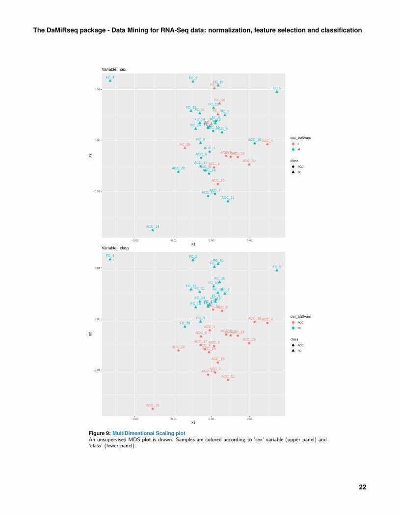
MultiDimensional Scaling (MDS) plots - MDS plot, drawn by ggplot2 package [16], pro-vides a visual representation of pattern of proximities (e.g. similarities or distances)among a set of samples, and allows the identification of natural clusters. For the ’class’and for each variable a MDS plot is drawn.
Relative Log Expression (RLE) boxplot - This plot, drawn by EDASeq package [17], helpsto visualize the differences between the distributions across samples: medians of eachRLE boxplot should be ideally centered around zero and a large shift from zero suggeststhat samples could have quality problems. Here, different colors means different classes.
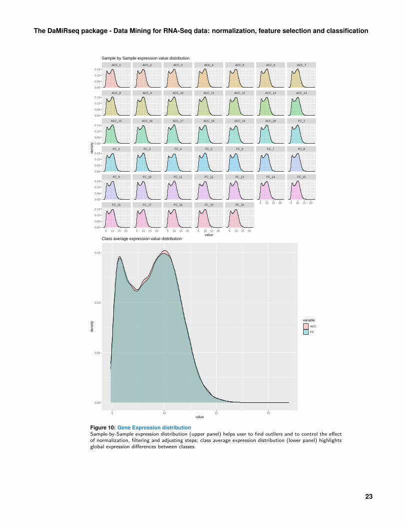
Sample-by-Sample expression distribution - This plot, drawn by ggplot2 package, helpsto visualize the differences between the real expression distributions across samples:shapes of every samples should be the same; indeed, samples with unusual shapes arelikely outliers.
Average expression distribution by class - This plot, drawn by ggplot2 package, helps tovisualize the differences between the average expression distribution for each class.
In this vignette, DaMiR.Allplot is used to appreciate the effect of data adjusting (see Sec-tion 3.4). First, we check how data appear just after normalization: the heatmap and RLEplot in Figure 3 (upper and lower panel, respectively) and MDS plots in Figures 4 and 5 donot highlight the presence of specific clusters.Note. If a variable contains missing data (i.e. “NA” values), the function cannot draw theplot showing variable information. The user is, however, encouraged to impute missing dataif s/he considers it meaningful to plot the covariate of interest.# After gene filtering and normalization
DaMiR.Allplot(data_filt, colData(data_filt))
13

The DaMiRseq package - Data Mining for RNA-Seq data: normalization, feature selection and classification
The df argument has been supplied using colData() function that returns the data frameof covariates stored into the “data_filt” object. Here, we used all the variables included intothe data frame (e.g. center, sex, age, death and class), although it is possible to use only asubset of them to be plotted.
14

The DaMiRseq package - Data Mining for RNA-Seq data: normalization, feature selection and classification
AC
C_15
AC
C_1
AC
C_8
FC
_11F
C_12
AC
C_13
FC
_18F
C_17
AC
C_5
FC
_8F
C_10
FC
_6A
CC
_14F
C_19
FC
_13F
C_15
AC
C_17
FC
_16A
CC
_7A
CC
_12A
CC
_18A
CC
_10A
CC
_11F
C_2
AC
C_20
FC
_3F
C_14
FC
_5A
CC
_19F
C_4
FC
_9A
CC
_16F
C_7
AC
C_4
AC
C_2
AC
C_3
FC
_20A
CC
_9A
CC
_6F
C_1
ACC_15ACC_1ACC_8FC_11FC_12ACC_13FC_18FC_17ACC_5FC_8FC_10FC_6ACC_14FC_19FC_13FC_15ACC_17FC_16ACC_7ACC_12ACC_18ACC_10ACC_11FC_2ACC_20FC_3FC_14FC_5ACC_19FC_4FC_9ACC_16FC_7ACC_4ACC_2ACC_3FC_20ACC_9ACC_6FC_1
centersexagedeathclass class
ACCFC
death4
1
age20−2930−3940−4950−5960−6970−79
sexFM
centerB1, A1C1, A1
0
0.02
0.04
0.06
0.08
0.1
0.12
0.14
−0.2
−0.1
0.0
0.1
0.2
Relative Log Expression
AC
C_1
AC
C_2
AC
C_3
AC
C_4
AC
C_5
AC
C_6
AC
C_7
AC
C_8
AC
C_9
AC
C_1
0A
CC
_11
AC
C_1
2A
CC
_13
AC
C_1
4A
CC
_15
AC
C_1
6A
CC
_17
AC
C_1
8A
CC
_19
AC
C_2
0F
C_1
FC
_2F
C_3
FC
_4F
C_5
FC
_6F
C_7
FC
_8F
C_9
FC
_10
FC
_11
FC
_12
FC
_13
FC
_14
FC
_15
FC
_16
FC
_17
FC
_18
FC
_19
FC
_20
Figure 3: Heatmap and RLEHeatmap (upper panel): colors in heatmap highlight the distance matrix, obtained by Spearman’s corre-lation metric: color gradient ranges from dark green, meaning ’minimum distance’ (i.e. dissimilarity = 0,correlation = 1), to light green green. On the top of heatmap, horizontal bars represent class and covari-ates. Each variable is differently colored (see legend). On the top and on the left side of the heatmap thedendrograms are drawn. Clusters can be easily identified.RLE (lower panel): a boxplot of the distribution of expression values computed as the difference betweenthe expression of each gene and the median expression of that gene accross all samples. Here, since allmedians are very close to zero, it appears that all the samples are well-normalized and do not present anyquality problems.
15

The DaMiRseq package - Data Mining for RNA-Seq data: normalization, feature selection and classification
ACC_1ACC_2
ACC_3
ACC_4
ACC_5
ACC_6
ACC_7
ACC_8
ACC_9
ACC_10
ACC_11
ACC_12
ACC_13
ACC_14ACC_15
ACC_16
ACC_17
ACC_18
ACC_19
ACC_20FC_1
FC_2
FC_3
FC_4
FC_5
FC_6
FC_7
FC_8
FC_9
FC_10
FC_11
FC_12
FC_13
FC_14
FC_15FC_16
FC_17FC_18
FC_19
FC_20
−0.050
−0.025
0.000
0.025
−0.04 0.00 0.04 0.08X1
X2
cov_list$Vars
a
a
B1, A1
C1, A1
class
ACC
FC
Variable: center
ACC_1ACC_2
ACC_3
ACC_4
ACC_5
ACC_6
ACC_7
ACC_8
ACC_9
ACC_10
ACC_11
ACC_12
ACC_13
ACC_14ACC_15
ACC_16
ACC_17
ACC_18
ACC_19
ACC_20FC_1
FC_2
FC_3
FC_4
FC_5
FC_6
FC_7
FC_8
FC_9
FC_10
FC_11
FC_12
FC_13
FC_14
FC_15FC_16
FC_17FC_18
FC_19
FC_20
−0.050
−0.025
0.000
0.025
−0.04 0.00 0.04 0.08X1
X2
1
2
3
4cov_list$Vars
class
ACC
FC
Variable: death
Figure 4: MultiDimentional Scaling plotAn unsupervised MDS plot is drawn. Samples are colored according to the ’Hardy death scale’ (upperpanel) and the ’center’ variable (lower panel).
16

The DaMiRseq package - Data Mining for RNA-Seq data: normalization, feature selection and classification
ACC_1ACC_2
ACC_3
ACC_4
ACC_5
ACC_6
ACC_7
ACC_8
ACC_9
ACC_10
ACC_11
ACC_12
ACC_13
ACC_14ACC_15
ACC_16
ACC_17
ACC_18
ACC_19
ACC_20FC_1
FC_2
FC_3
FC_4
FC_5
FC_6
FC_7
FC_8
FC_9
FC_10
FC_11
FC_12
FC_13
FC_14
FC_15FC_16
FC_17FC_18
FC_19
FC_20
−0.050
−0.025
0.000
0.025
−0.04 0.00 0.04 0.08X1
X2
cov_list$Vars
a
a
F
M
class
ACC
FC
Variable: sex
ACC_1ACC_2
ACC_3
ACC_4
ACC_5
ACC_6
ACC_7
ACC_8
ACC_9
ACC_10
ACC_11
ACC_12
ACC_13
ACC_14ACC_15
ACC_16
ACC_17
ACC_18
ACC_19
ACC_20FC_1
FC_2
FC_3
FC_4
FC_5
FC_6
FC_7
FC_8
FC_9
FC_10
FC_11
FC_12
FC_13
FC_14
FC_15FC_16
FC_17FC_18
FC_19
FC_20
−0.050
−0.025
0.000
0.025
−0.04 0.00 0.04 0.08X1
X2
cov_list$Vars
a
a
ACC
FC
class
ACC
FC
Variable: class
Figure 5: MultiDimentional Scaling plotAn unsupervised MDS plot is drawn. Samples are colored according to ’sex’ variable (upper panel) and’class’ (lower panel).
17
The DaMiRseq package - Data Mining for RNA-Seq data: normalization, feature selection and classification
FC_16 FC_17 FC_18 FC_19 FC_20
FC_9 FC_10 FC_11 FC_12 FC_13 FC_14 FC_15
FC_2 FC_3 FC_4 FC_5 FC_6 FC_7 FC_8
ACC_15 ACC_16 ACC_17 ACC_18 ACC_19 ACC_20 FC_1
ACC_8 ACC_9 ACC_10 ACC_11 ACC_12 ACC_13 ACC_14
ACC_1 ACC_2 ACC_3 ACC_4 ACC_5 ACC_6 ACC_7
5 10 15 20 25 5 10 15 20 25 5 10 15 20 25 5 10 15 20 25 5 10 15 20 25
5 10 15 20 25 5 10 15 20 25
0.00
0.05
0.10
0.15
0.00
0.05
0.10
0.15
0.00
0.05
0.10
0.15
0.00
0.05
0.10
0.15
0.00
0.05
0.10
0.15
0.00
0.05
0.10
0.15
value
dens
ity
Sample by Sample expression value distribution
0.00
0.05
0.10
0.15
5 10 15 20value
dens
ity
variable
ACC
FC
Class average expression value distribution
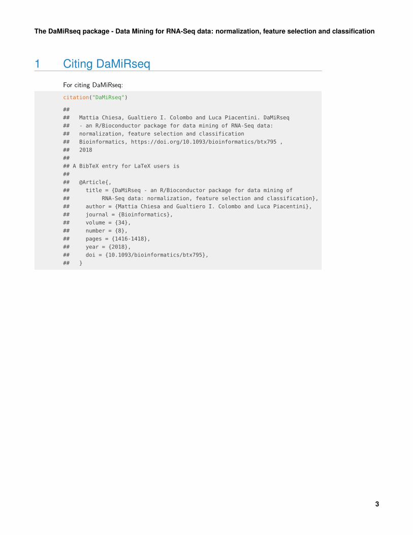
Figure 6: Gene Expression distributionSample-by-Sample expression distribution (upper panel) helps user to find outliers and to control the effectof normalization, filtering and adjusting steps; class average expression distribution (lower panel) highlightsglobal expression differences between classes.
18

The DaMiRseq package - Data Mining for RNA-Seq data: normalization, feature selection and classification
After removing the effect of “noise” from our expression data, as presented in Section 3.4,we may appreciate the result of data adjustiment for sv: now, the heatmap in Figure 7 andMDS plots in Figures 8 and 9 exhibit specific clusters related to ’class’ variable. Moreover,the effect on data distribution is irrelevant: both RLE in Figures 3 and 7 show minimal shiftsfrom the zero line, whereas RLE of adjusted data displays lower dispersion.# After sample filtering and sv adjusting
DaMiR.Allplot(data_adjust, colData(data_adjust))
19

The DaMiRseq package - Data Mining for RNA-Seq data: normalization, feature selection and classification
FC
_5F
C_20
FC
_2F
C_10
AC
C_9
FC
_14F
C_7
FC
_9A
CC
_14F
C_19
FC
_1F
C_11
FC
_13F
C_15
FC
_12F
C_3
FC
_16F
C_6
FC
_8F
C_17
AC
C_16
AC
C_6
AC
C_10
AC
C_4
AC
C_2
AC
C_13
FC
_18F
C_4
AC
C_19
AC
C_17
AC
C_20
AC
C_7
AC
C_11
AC
C_5
AC
C_8
AC
C_12
AC
C_18
AC
C_1
AC
C_3
AC
C_15
FC_5FC_20FC_2FC_10ACC_9FC_14FC_7FC_9ACC_14FC_19FC_1FC_11FC_13FC_15FC_12FC_3FC_16FC_6FC_8FC_17ACC_16ACC_6ACC_10ACC_4ACC_2ACC_13FC_18FC_4ACC_19ACC_17ACC_20ACC_7ACC_11ACC_5ACC_8ACC_12ACC_18ACC_1ACC_3ACC_15
centersexagedeathclass class
ACCFC
death4
1
age20−2930−3940−4950−5960−6970−79
sexFM
centerB1, A1C1, A1
0
0.01
0.02
0.03
0.04
−0.10
−0.05
0.00
0.05
0.10
Relative Log Expression
AC
C_1
AC
C_2
AC
C_3
AC
C_4
AC
C_5
AC
C_6
AC
C_7
AC
C_8
AC
C_9
AC
C_1
0A
CC
_11
AC
C_1
2A
CC
_13
AC
C_1
4A
CC
_15
AC
C_1
6A
CC
_17
AC
C_1
8A
CC
_19
AC
C_2
0F
C_1
FC
_2F
C_3
FC
_4F
C_5
FC
_6F
C_7
FC
_8F
C_9
FC
_10
FC
_11
FC
_12
FC
_13
FC
_14
FC
_15
FC
_16
FC
_17
FC
_18
FC
_19
FC
_20
Figure 7: Heatmap and RLEHeatmap (upper panel): colors in heatmap highlight the distance matrix, obtained by Spearman’s corre-lation metric: color gradient ranges from dark green, meaning ’minimum distance’ (i.e. dissimilarity = 0,correlation = 1), to light green green. On the top of heatmap, horizontal bars represent class and variables.Each variable is differently colored (see legend). The two dendrograms help to quickly identify clusters.RLE (lower panel): Relative Log Expression boxplot. A boxplot of the distribution of expression valuescomputed as the difference between the expression of each gene and the median expression of that geneaccross all samples is shown. Here, all medians are very close to zero, meaning that samples are well-normalized.
20

The DaMiRseq package - Data Mining for RNA-Seq data: normalization, feature selection and classification
ACC_1ACC_2
ACC_3
ACC_4
ACC_5
ACC_6
ACC_7
ACC_8
ACC_9
ACC_10
ACC_11
ACC_12
ACC_13
ACC_14
ACC_15
ACC_16
ACC_17
ACC_18
ACC_19
ACC_20
FC_1
FC_2
FC_3
FC_4
FC_5
FC_6
FC_7
FC_8
FC_9FC_10
FC_11FC_12
FC_13
FC_14
FC_15
FC_16FC_17
FC_18
FC_19
FC_20
−0.01
0.00
0.01
−0.02 −0.01 0.00 0.01X1
X2
cov_list$Vars
a
a
B1, A1
C1, A1
class
ACC
FC
Variable: center
ACC_1ACC_2
ACC_3
ACC_4
ACC_5
ACC_6
ACC_7
ACC_8
ACC_9
ACC_10
ACC_11
ACC_12
ACC_13
ACC_14
ACC_15
ACC_16
ACC_17
ACC_18
ACC_19
ACC_20
FC_1
FC_2
FC_3
FC_4
FC_5
FC_6
FC_7
FC_8
FC_9FC_10
FC_11FC_12
FC_13
FC_14
FC_15
FC_16FC_17
FC_18
FC_19
FC_20
−0.01
0.00
0.01
−0.02 −0.01 0.00 0.01X1
X2
1
2
3
4cov_list$Vars
class
ACC
FC
Variable: death
Figure 8: MultiDimentional Scaling plotAn unsupervised MDS plot is drawn. Samples are colored according to the ’Hardy death scale’ (upperpanel) and the ’center’ variable (lower panel).
21
The DaMiRseq package - Data Mining for RNA-Seq data: normalization, feature selection and classification
ACC_1ACC_2
ACC_3
ACC_4
ACC_5
ACC_6
ACC_7
ACC_8
ACC_9
ACC_10
ACC_11
ACC_12
ACC_13
ACC_14
ACC_15
ACC_16
ACC_17
ACC_18
ACC_19
ACC_20
FC_1
FC_2
FC_3
FC_4
FC_5
FC_6
FC_7
FC_8
FC_9FC_10
FC_11FC_12
FC_13
FC_14
FC_15
FC_16FC_17
FC_18
FC_19
FC_20
−0.01
0.00
0.01
−0.02 −0.01 0.00 0.01X1
X2
cov_list$Vars
a
a
F
M
class
ACC
FC
Variable: sex
ACC_1ACC_2
ACC_3
ACC_4
ACC_5
ACC_6
ACC_7
ACC_8
ACC_9
ACC_10
ACC_11
ACC_12
ACC_13
ACC_14
ACC_15
ACC_16
ACC_17
ACC_18
ACC_19
ACC_20
FC_1
FC_2
FC_3
FC_4
FC_5
FC_6
FC_7
FC_8
FC_9FC_10
FC_11FC_12
FC_13
FC_14
FC_15
FC_16FC_17
FC_18
FC_19
FC_20
−0.01
0.00
0.01
−0.02 −0.01 0.00 0.01X1
X2
cov_list$Vars
a
a
ACC
FC
class
ACC
FC
Variable: class
Figure 9: MultiDimentional Scaling plotAn unsupervised MDS plot is drawn. Samples are colored according to ’sex’ variable (upper panel) and’class’ (lower panel).
22
The DaMiRseq package - Data Mining for RNA-Seq data: normalization, feature selection and classification
FC_16 FC_17 FC_18 FC_19 FC_20
FC_9 FC_10 FC_11 FC_12 FC_13 FC_14 FC_15
FC_2 FC_3 FC_4 FC_5 FC_6 FC_7 FC_8
ACC_15 ACC_16 ACC_17 ACC_18 ACC_19 ACC_20 FC_1
ACC_8 ACC_9 ACC_10 ACC_11 ACC_12 ACC_13 ACC_14
ACC_1 ACC_2 ACC_3 ACC_4 ACC_5 ACC_6 ACC_7
5 10 15 20 5 10 15 20 5 10 15 20 5 10 15 20 5 10 15 20
5 10 15 20 5 10 15 20
0.00
0.05
0.10
0.15
0.00
0.05
0.10
0.15
0.00
0.05
0.10
0.15
0.00
0.05
0.10
0.15
0.00
0.05
0.10
0.15
0.00
0.05
0.10
0.15
value
dens
ity
Sample by Sample expression value distribution
0.00
0.05
0.10
0.15
5 10 15 20value
dens
ity
variable
ACC
FC
Class average expression value distribution
Figure 10: Gene Expression distributionSample-by-Sample expression distribution (upper panel) helps user to find outliers and to control the effectof normalization, filtering and adjusting steps; class average expression distribution (lower panel) highlightsglobal expression differences between classes.
23

The DaMiRseq package - Data Mining for RNA-Seq data: normalization, feature selection and classification
3.6 Exporting output data
DaMiRseq has been designed to allow users to export the outputs of each function, whichconsist substantially in matrix or data.frame objects. Export can be done, using the base Rfunctions, such as write.table or write.csv. For example, we could be interested in savingnormalized data matrix, stored in “data_norm” in a tab-delimited file:outputfile <- "DataNormalized.txt"
write.table(data_norm, file = outputfile_norm, quote = FALSE, sep = "\t")
24
The DaMiRseq package - Data Mining for RNA-Seq data: normalization, feature selection and classification
4 Two specific supervised machine learning workflows
As we described in the previuos sections, RNA-Seq experiments, are used to generate hundredsto thousand of features at once. However, most of them are non informative to discriminatephenotypes and useless for further investigations.In this context, supervised machine learning is a powerful tool that gathers several algorithms,to select the most informative features in high-dimensional data and design accurate predic-tion models. To achieve these aims, the supervised learning algorithms need ’labeled data’,where each observation of the dataset comes with a priori knowledge of the class member-ship.Since version 2.0.0 of the software, DaMiRseq offers a solution to solve two distinct problems,in supervised learning analysis: (i) finding a small set of robust features, and (ii) building themost reliable model to predict new samples.
• Finding a small set of robust features to discriminate classes.This task seeks to select and assess the reliability of a feature set from high-dimensionaldata. Specifically, we first implemented a 4-step feature selection strategy (orange boxin Figure 11, panel A), in order to get the most relevant features. Then, we testedthe robustness of the selected features by performing a bootstrap strategy, in which an’ensemble learner’ classifier is built for each iteration (green box in Figure 11, panel A).In Section 4.1, we described this analysis in details.
• Building the most reliable model to predict new samples.An important goal in machine learning is to develop a mathematical model, able tocorrectly associate each observation to the corresponding class. This model, also knownas classification or prediction model (Figure 11, panel B), aimed at ensuring the highestprediction accuracy with as few features as possible.First, several different models are generate by iteratively (i) splitting data in trainingand validation sets; (ii) performing feature selection on the training set (orange box inFigure 11, panel B); (iii) building a classification model on the training set (pink boxin Figure 11, panel B); and, (iv) testing the classification model on the validation set(purple box in Figure 11, panel B). Finally, taking into account the performance of allgenerated models, the most reliable one is selected (red box in Figure 11, panel B).This model will be used for any further prediction on independent test sets (light bluebox in Figure 11, panel B). We will refer to this model as ’optimal model’.In Section 4.2, we thoroughly described how to perform this analysis.
25

The DaMiRseq package - Data Mining for RNA-Seq data: normalization, feature selection and classification
Resampling(Cross-Validation/Bootstrap)
Overall Classification
DaMiR.EnsembleLearning
Feature SelectionDaMiR.FSelectDaMiR.FReductDaMiR.FSortDaMiR.FBest
Output• Averaged classification performance calculated
on a dataset with selected features;• Robustness evaluation of a feature set;
Independent Test Set
Training Set Validation Set
Feature Selection
DaMiR.FSelectDaMiR.FReductDaMiR.FSortDaMiR.FBest
Model Training
DaMiR.EnsL_Train
Model TestDaMiR.EnsL_Test
Best Model SelectionDaMiR.ModelSelect
Prediction on new dataDaMiR.EnsL_Predict
Dataset
Output• Performance for each resampling iteration;• A single optimal prediction model;
A BAim
Finding a small set of robust features, to discriminate classes.
AimFinding the optimal model to
predict new samples.
fold-1
fold-(N-1)fold-N
Dataset
fold-i
Figure 11: The DaMiRseq machine learning workflowsEach elliptic box represents a specific step, where the aims and the corresponding functions are specified.In panel A, we provided the workflow to find a small set of informative features, described in Section 4.1.In panel B, we provided the workflow to find the best prediction model, described in Section 4.2.
4.1 Finding a small set of informative, robust features
This Section, where we will describe how to get a small set of robust features from anRNA-Seq dataset, is organized in two parts: in Section 4.1.1, all the feature selection stepsand the corresponding functions are reported in detail; while, in Section 4.1.2 we will focuson the classification step that we performed for assessing the robustness of the feature set.Mathematical details about the classifier implementation are also provided.
4.1.1 Feature Selection
The steps implemented in the Section 3 returned a fully filtered, normalized, adjusted expres-sion matrix with the effect of sv removed. However, the number of features in the dataset isstill high and greatly exceeds the number of observations. We have to deal, here, with thewell-known issue for high-dimensional data known as the “curse of dimensionality”. Addingnoise features that are not truly associated with the response (i.e. class) may lead, in fact,to a worsening model accuracy. In this situation, the user needs to remove those featuresthat bear irrelevant or redundant information. The feature selection technique implementedhere does not alter the original representation of the variables, but simply selects a subset ofthem. It includes three different steps briefly described in the following paragraphs.
Variable selection in Partial Least Squares (PLS) The first step allows the user toexclude all non-informative class-related features using a backward variable elimination pro-cedure [18]. The DaMiR.FSelect function embeds a principal component analysis (PCA) to
26

The DaMiRseq package - Data Mining for RNA-Seq data: normalization, feature selection and classification
identify principal components (PCs) that correlate with “class”. The correlation coefficientis defined by the user through the th.corr argument. The higher the correlation, the lowerthe number of PCs returned. Importantly, users should pay attention to appropriately setthe th.corr argument since the total number of retrieved features depends, indeed, on thenumber of the selected PCs.The number of class-correlated PCs is then internally used by the function to perform abackward variable elimination-PLS and remove those variables that are less informative withrespect to class [19].Note. Before running the DaMiR.FSelect function, we need to transpose our normalizedexpression data. It can be done by the base R function t(). However, we implemented thehelper function DaMiR.transpose that transposes the data but also tries to prevent the useof tricky feature labels. The “-” and “.” characters within variable labels (commonly found,for example, in gene symbols) may, in fact, cause errors if included in the model design asit is required to execute part of the code of the DaMiR.FSelect function. Thus, we, firstly,search and, eventually, replace them with non causing error characters.We used the set.seed(12345) function that allows the user to make the results of the wholepipeline reproducible.set.seed(12345)
data_clean<-DaMiR.transpose(assay(data_adjust))
df<-colData(data_adjust)
data_reduced <- DaMiR.FSelect(data_clean, df, th.corr=0.4)
## You are performing feature selection on a binary class object.
## 19049 Genes have been discarded for classification 294 Genes remained.
The “data_reduced” object returns an expression matrix with potentially informative features.In our case study, the initial number of 19052 features has been reduced to 274.
Removing highly correlated features Some of the returned informative features may,however, be highly correlated. To prevent the inclusion of redundant features that maydecrease the model performance during the classification step, we apply a function thatproduces a pair-wise absolute correlation matrix. When two features present a correlationhigher than th.corr argument, the algorithm calculates the mean absolute correlation ofeach feature and, then, removes the feature with the largest mean absolute correlation.data_reduced <- DaMiR.FReduct(data_reduced$data)
## 66 Highly correlated features have been discarded for classification.
## 228 Features remained.
DaMiR.MDSplot(data_reduced, df)
In our example, we used a Spearman’s correlation metric and a correletion threshold of 0.85(default). This reduction step filters out 54 highly correlated genes from the 274 returned bythe DaMiR.FSelect. The figure below shows the MDS plot drawn by the use of the expressionmatrix of the remaining 220 genes.
27

The DaMiRseq package - Data Mining for RNA-Seq data: normalization, feature selection and classification
ACC_1
ACC_2
ACC_3
ACC_4
ACC_5
ACC_6
ACC_7ACC_8
ACC_9
ACC_10
ACC_11 ACC_12
ACC_13
ACC_14
ACC_15
ACC_16
ACC_17
ACC_18
ACC_19
ACC_20
FC_1
FC_2
FC_3
FC_4
FC_5
FC_6
FC_7
FC_8
FC_9
FC_10
FC_11
FC_12
FC_13
FC_14
FC_15
FC_16
FC_17
FC_18
FC_19
FC_20
−0.05
0.00
0.05
−0.1 0.0 0.1 0.2X1
X2
class
a
a
ACC
FC
Figure 12: MultiDimentional Scaling plotA MDS plot is drawn, considering only most informative genes, obtained after feature selection: color codeis referred to ’class’.
Ranking and selecting most relevant features The above functions produced a reducedmatrix of variables. Nonetheless, the number of reduced variables might be too high to providefaster and cost-effective classification models. Accordingly, we should properly select a subsetof the most informative features. The DaMiR.FSort function implements a procedure to rankfeatures by their importance. The method implements a multivariate filter technique (i.e.RReliefF ) that assessess the relevance of features (for details see the relief function of theFSelector package) [20, 21]. The function produced a data frame with two columns, whichreports features ranked by importance scores: a RReliefF score and scaled.RReliefF value;the latter is computed in this package to implement a “z-score” standardization procedureon RReliefF values.Note. This step may be time-consuming if a data matrix with a high number of features isused as input. We observed, in fact, that there is a quadratic relationship between executiontime of the algorithm and the number of features. The user is advised with a message aboutthe estimated time needed to compute the score and rank the features. Thus, we stronglysuggest to filter out non informative features by the DaMiR.FSelect and DaMiR.FReduct
functions before performing this step.# Rank genes by importance:
df.importance <- DaMiR.FSort(data_reduced, df)
## Please wait. This operation will take about 43 seconds (i.e. about 1 minutes).
head(df.importance)
## RReliefF scaled.RReliefF
## ENSG00000164326 0.3225314 3.517307
28

The DaMiRseq package - Data Mining for RNA-Seq data: normalization, feature selection and classification
## ENSG00000140015 0.3106650 3.343058
## ENSG00000131378 0.2598680 2.597137
## ENSG00000151892 0.2596646 2.594150
## ENSG00000137699 0.2584838 2.576811
## ENSG00000258754 0.2504452 2.458770
After the importance score is calculated, a subset of features can be selected and used aspredictors for classification purpose. The function DaMiR.FBest is used to select a smallsubset of predictors:# Select Best Predictors:
selected_features <- DaMiR.FBest(data_reduced, ranking=df.importance,
n.pred = 5)
## 5 Predictors have been selected for classification
selected_features$predictors
## [1] "ENSG00000164326" "ENSG00000140015" "ENSG00000131378" "ENSG00000151892"
## [5] "ENSG00000137699"
# Dendrogram and heatmap:
DaMiR.Clustplot(selected_features$data, df)
Here, we selected the first 5 genes (default) ranked by importance.Note. The user may also wish to select “automatically” (i.e. not defined by the user) thenumber of important genes. This is possible by setting autoselect="yes" and a thresholdfor the scaled.RReliefF, i.e. th.zscore argument. These normalized values (rescaled to havea mean of 0 and standard deviation of 1) make it possible to compare predictors rankingobtained by running the pipeline with different parameters. Further information about the’feature selection’ step and comparison with other methods can be found in the SupplementaryArticle Data by Chiesa et al. [12] with an example code. In adition, an example of the effectiveuse of our feature selection process has been obtained for the detection of P. aeruginosatranscriptional signature of Human Infection in Cornforth et al. [22].
29

The DaMiRseq package - Data Mining for RNA-Seq data: normalization, feature selection and classification
ENSG00000153266ENSG00000182366ENSG00000144152ENSG00000138100ENSG00000162733ENSG00000263724ENSG00000243742ENSG00000225889ENSG00000233670ENSG00000006128ENSG00000124134ENSG00000179520ENSG00000250303ENSG00000103154ENSG00000101180ENSG00000108960ENSG00000183287ENSG00000198963ENSG00000144550ENSG00000153820ENSG00000134207ENSG00000178342ENSG00000057294ENSG00000165606ENSG00000150394ENSG00000228214ENSG00000141738ENSG00000122375ENSG00000147041ENSG00000106852ENSG00000156219ENSG00000149305ENSG00000223573ENSG00000150361ENSG00000077327ENSG00000131885ENSG00000273036ENSG00000152527ENSG00000144407ENSG00000250685ENSG00000186212ENSG00000143473ENSG00000118898ENSG00000105976ENSG00000258754ENSG00000137699ENSG00000151892ENSG00000131378ENSG00000140015ENSG00000164326Top50 features
0.15 0.20 0.25 0.30
Attributes importance by RReliefF
RReliefF importance
Figure 13: Feature Importance PlotThe dotchart shows the list of top 50 genes, sorted by RReliefF importance score. This plot may be used toselect the most important predictors to be used for classification.
30

The DaMiRseq package - Data Mining for RNA-Seq data: normalization, feature selection and classification
FC
_10F
C_19
FC
_1F
C_7
FC
_20F
C_6
FC
_5F
C_9
FC
_3F
C_12
FC
_16F
C_2
FC
_15F
C_18
FC
_13F
C_17
FC
_8F
C_11
AC
C_4
AC
C_10
AC
C_16
AC
C_20
AC
C_2
AC
C_13
AC
C_5
AC
C_6
AC
C_7
AC
C_11
AC
C_12
AC
C_15
AC
C_1
AC
C_3
AC
C_17
AC
C_18
FC
_4A
CC
_9F
C_14
AC
C_19
AC
C_8
AC
C_14
ENSG00000164326
ENSG00000131378
ENSG00000140015
ENSG00000151892
ENSG00000137699
centersexagedeathclass class
ACCFC
death4
1
age20−2930−3940−4950−5960−6970−79
sexFM
centerB1, A1C1, A1
−2
−1
0
1
2
Figure 14: ClustergramThe clustergram is generated by using the expression values of the 5 predictors selected by DaMiR.FBest
function. As for the heatmap generated by DaMiR.Allplot, ’class’ and covariates are drawn as horizontaland color coded bars.
31
The DaMiRseq package - Data Mining for RNA-Seq data: normalization, feature selection and classification
4.1.2 Classification
All the steps executed so far allowed the reduction of the original expression matrix; theobjective is to capture a subset of original data as informative as possible, in order to carryout a classification analysis. In this paragraph, we describe the statistical learning strategywe implemented to tackle both binary and multi-class classification problems.A meta-learner is built, combining up to 8 different classifiers through a “Stacking” strategy.Currently, there is no gold standard for creating the best rule to combine predictions [6]. Wedecided to implement a framework that relies on the “weighted majority voting” approach[23]. In particular, our method estimates a weight for each used classifier, based on its ownaccuracy, and then use these weights, together with predictions, to fine-tune a decision rule(i.e. meta-learner). Briefly, first a training set (TR1) and a test set (TS1) are generatedby “Bootstrap” sampling. Then, sampling again from subset TR1, another pair of training(TR2) and test set (TS2) were obtained. TR2 is used to train RF, NB, SVM, 3kNN, LDA,NN, PLS and/or LR classifiers (the number and the type are chosen by the user), whereasTS2 is used to test their accuracy and to calculate weights (w) by formula:
wclassifieri =Accuracyclassifieri
N∑j=1
Accuracyclassifierj
1
where i is a specific classifiers and N is the total number of them (here, N <= 8). Usingthis approach:
N∑i=1
wi = 1 2
The higher the value of wi, the more accurate is the classifier.The performance of the meta-learner (labelled as “Ensemble”) is evaluated by using TS1. Thedecision rule of the meta-learner is made by a linear combination of the products betweenweigths (w) and predictions (Pr) of each classifier; for each sample k, the prediction iscomputed by:
Pr(k,Ensemble) =
N∑i=1
wi ∗ Pr(k,classifieri) 3
Pr(k,Ensemble) ranges from 0 to 1. For binary classification analysis, 0 means high proba-bility to belong to one class, while 1 means high probability to belong to the other class);predictions close to 0.5 have to be considered as made by chance. For multi-class analysis1 means right prediction, while 0 means wrong prediction. This process is repeated severaltimes to assess the robustness of the set of predictors used.
The above mentioned procedure is implemented in the DaMiR.EnsembleLearning function,where fSample.tr, fSample.tr.w and iter arguments allow the algorithm tuning.This function performs a Bootstrap resampling strategy with iter iterations, in which severalmeta-classifiers are built and tested, by generating iter training sets and iter test sets in arandom way. Then each classification metrics (acc,sen) is calculated on the iter test sets.Finally, the average performance (and standard deviation) is provided (text and violin plots).To speed up the execution time of the function, we set iter = 30 (default is 100) but wesuggest to use an higher number of iterations to obtain more accurate results. The function
32

The DaMiRseq package - Data Mining for RNA-Seq data: normalization, feature selection and classification
returns a list containing the matrix of accuracies of each classifier in each iteration and, inthe case of a binary classification problem, the specificity, the sensitivity, PPV, NPV and theMatthew’s Correlation Coefficient (MCC). These objects can be accessed using the $ accessor.
Classification_res <- DaMiR.EnsembleLearning(selected_features$data,
classes=df$class, fSample.tr = 0.5,
fSample.tr.w = 0.5, iter = 30)
## You select: RF LR kNN LDA NB SVM weak classifiers for creating
## the Ensemble meta-learner.
## Ensemble classification is running. 30 iterations were chosen:
## Accuracy [%]:
## Ensemble RF SVM NB LDA LR kNN
## Mean: 0.95 0.95 0.97 0.94 0.91 0.96 0.95
## St.Dev. 0.03 0.04 0.03 0.04 0.08 0.02 0.04
## MCC score:
## Ensemble RF SVM NB LDA LR kNN
## Mean: 0.91 0.9 0.93 0.89 0.83 0.92 0.9
## St.Dev. 0.06 0.07 0.06 0.08 0.15 0.05 0.07
## Specificity:
## Ensemble RF SVM NB LDA LR kNN
## Mean: 0.96 0.96 0.98 0.91 0.91 0.96 0.94
## St.Dev. 0.05 0.05 0.04 0.07 0.09 0.05 0.06
## Sensitivity:
## Ensemble RF SVM NB LDA LR kNN
## Mean: 0.96 0.95 0.96 0.98 0.93 0.96 0.96
## St.Dev. 0.05 0.05 0.05 0.04 0.09 0.05 0.05
## PPV:
## Ensemble RF SVM NB LDA LR kNN
## Mean: 0.95 0.95 0.98 0.9 0.9 0.96 0.94
## St.Dev. 0.06 0.05 0.05 0.09 0.1 0.05 0.06
## NPV:
## Ensemble RF SVM NB LDA LR kNN
## Mean: 0.95 0.94 0.96 0.98 0.93 0.96 0.96
## St.Dev. 0.06 0.06 0.06 0.05 0.1 0.05 0.06
33

The DaMiRseq package - Data Mining for RNA-Seq data: normalization, feature selection and classification
0.6
0.7
0.8
0.9
1.0
Ensemble RF SVM NB LDA LR kNNClassifiers
Acc
urac
y
factor(Classifiers)
Ensemble
RF
SVM
NB
LDA
LR
kNN
Figure 15: Accuracies ComparisonThe violin plot highlights the classification accuracy of each classifier, computed at each iteration; a blackdot represents a specific accuracy value while the shape of each “violin” is drawn by a Gaussian kernel den-sity estimation. Averaged accuracies and standard deviations are represented by white dots and lines.
As shown in Figure 15 almost all single, weak classifiers show high or very high classificationperformancies, in terms of accuracy, specificity, sensitivity and MCC.
Figure 15 highlights that the five selected features ensured high and reproducible performance,whatever the classifier; indeed, the average accuracy wass always greater than 90% andpperformance deviated by no more than 4% from the mean value.
4.2 Building the optimal prediction model
In this section, we present the workflow to generate an effective classification model thatcan be later used to predict the class membership of new samples. Basically, DaMiRseqimplements a supervised learning procedure, depicted in Figure 11, panel B, where each stepis performed by a specific function.Indeed, the DaMiR.EnsL_Train and the DaMiR.EnsL_Test functions allow training and testingone single model at once, respectively.The DaMiR.ModelSelect function implements six strategies to perform the model selection,taking into account a particular classification metrics (e.g., Accuracy) along with the numberof predictors. The idea behind this function is to search for the most reliable model ratherthan the best ever; this should help to avoid over-fitted training data, leading to poor per-formance in further predictions.Users can choose a specific strategy, combining one of the three value of the type.sel ar-
34

The DaMiRseq package - Data Mining for RNA-Seq data: normalization, feature selection and classification
gument (type.sel = c("mode", "median", "greater") and one of the two values of thenpred.sel argument (npred.sel = c("min", "rnd"). Let us assume we generated N dif-ferent model during a resampling strategy, each one characterized by a certain accuracy andnumber of selected features. Then, the combination of:
• type.sel = "mode" and npred.sel = "min", will select the model with minimum num-ber of features, among those with the accuracy equal to the mode (i.e., the mostfrequent value) of all N accuracies;
• type.sel = "mode" and npred.sel = "rnd", will select randomly one model, amongthose with the accuracy equal to the mode (i.e., the most frequent value) of all Naccuracies;
• type.sel = "median" and npred.sel = "min", will select the model with minimumnumber of features, among those with the accuracy equal to the median of all Naccuracies;
• type.sel = "median" and npred.sel = "rnd", will select randomly one model, amongthose with the accuracy equal to the median of all N accuracies;
• type.sel = "greater" and npred.sel = "min", will select the model with minimumnumber of features, among those with the accuracy greater than a fixed value, specifiedby th.sel;
• type.sel = "greater" and npred.sel = "rnd", will select randomly one model, amongthose with the accuracy greater than a fixed value, specified by th.sel;
Finally, the DaMiR.EnsL_Predict function allows performing the class prediction of new sam-ples.Note. Currently, DaMiR.EnsL_Train, DaMiR.EnsL_Test and DaMiR.EnsL_Predict work onlyon binary classification problems.
4.2.1 Training and testing inside the cross-validation
In order to simulate a typical genome-wide setting, we performed this analysis on the data_adjustdataset, which is composed of 40 samples (20 ACC and 20 FC) and 19343 features.First, we randomly selected 5 ACC and 5 FC samples (Test_set), which will be later usedfor the final prediction step. The remaining samples composed the case study dataset (Learning_set).# Dataset for prediction
set.seed(10101)
nSampl_cl1 <- 5
nSampl_cl2 <- 5
## May create unbalanced Learning and Test sets
# idx_test <- sample(1:ncol(data_adjust), 10)
# Create balanced Learning and Test sets
idx_test_cl1<-sample(1:(ncol(data_adjust)/2), nSampl_cl1)
idx_test_cl2<-sample(1:(ncol(data_adjust)/2), nSampl_cl2) + ncol(data_adjust)/2
idx_test <- c(idx_test_cl1, idx_test_cl2)
Test_set <- data_adjust[, idx_test, drop=FALSE]
35

The DaMiRseq package - Data Mining for RNA-Seq data: normalization, feature selection and classification
Learning_set <- data_adjust[, -idx_test, drop=FALSE]
Then, we implemented a 3-fold Cross Validation, as resampling strategy. Please, note thatthis choice is an unsuitable setting in every real machine learning analysis; therefore, westrongly recommend to adopt more effective resampling strategies, as bootstrap632 or 10-fold cross validation, to obtain more accurate results.
# Training and Test into a 'nfold' Cross Validation
nfold <- 3
cv_sample <- c(rep(seq_len(nfold), each=ncol(Learning_set)/(2*nfold)),
rep(seq_len(nfold), each=ncol(Learning_set)/(2*nfold)))
# Variables initialization
cv_models <- list()
cv_predictors <- list()
res_df <- data.frame(matrix(nrow = nfold, ncol = 7))
colnames(res_df) <- c("Accuracy",
"N.predictors",
"MCC",
"sensitivity",
"Specificty",
"PPV",
"NPV")
For each iteration, we (i) split the dataset in training (TR_set) and validation set (Val_set);(ii) performed the features selection and built the model (ensl_model) on the training set;and, (iii) tested and evaluated the model on the validation set (res_Val). Regarding thefeature selection, we used the DaMiRseq procedure, described in Section 4.1.1; however, anyother feature selection strategies can be jointly utilized, such as the GARS package.for (cv_fold in seq_len(nfold)){
# Create Training and Validation Sets
idx_cv <- which(cv_sample != cv_fold)
TR_set <- Learning_set[,idx_cv, drop=FALSE]
Val_set <- Learning_set[,-idx_cv, drop=FALSE]
#### Feature selection
data_reduced <- DaMiR.FSelect(t(assay(TR_set)),
as.data.frame(colData(TR_set)),
th.corr=0.4)
data_reduced <- DaMiR.FReduct(data_reduced$data,th.corr = 0.9)
df_importance <- DaMiR.FSort(data_reduced,
as.data.frame(colData(TR_set)))
selected_features <- DaMiR.FBest(data_reduced,
ranking=df_importance,
autoselect = "yes")
# update datasets
TR_set <- TR_set[selected_features$predictors,, drop=FALSE]
Val_set <- Val_set[selected_features$predictors,drop=FALSE]
36

The DaMiRseq package - Data Mining for RNA-Seq data: normalization, feature selection and classification
### Model building
ensl_model <- DaMiR.EnsL_Train(TR_set,
cl_type = c("RF", "LR"))
# Store all trained models
cv_models[[cv_fold]] <- ensl_model
### Model testing
res_Val <- DaMiR.EnsL_Test(Val_set,
EnsL_model = ensl_model)
# Store all ML results
res_df[cv_fold,1] <- res_Val$accuracy[1] # Accuracy
res_df[cv_fold,2] <- length(res_Val$predictors) # N. of predictors
res_df[cv_fold,3] <- res_Val$MCC[1]
res_df[cv_fold,4] <- res_Val$sensitivity[1]
res_df[cv_fold,5] <- res_Val$Specificty[1]
res_df[cv_fold,6] <- res_Val$PPV[1]
res_df[cv_fold,7] <- res_Val$NPV[1]
cv_predictors[[cv_fold]] <- res_Val$predictors
}
4.2.2 Selection and Prediction
Finally, we searched for the ’optimal model’ to be used for predicting new samples. In thissimulation, we set type.sel = "mode" and npred.sel = "min" to select the model with thelowest number of seleted features ensuring the most frequent accuracy value.# Model Selection
res_df[,1:5]
## Accuracy N.predictors MCC sensitivity Specificty
## 1 0.9 5 0.8164966 1.0000000 0.8333333
## 2 0.8 6 0.6546537 1.0000000 0.7142857
## 3 0.9 9 0.8164966 0.8333333 1.0000000
idx_best_model <- DaMiR.ModelSelect(res_df,
type.sel = "mode",
npred.sel = "min")
## In your df, the 'optimal model' has index: 1
## Accuracy = 0.9
## 5 predictors
37

The DaMiRseq package - Data Mining for RNA-Seq data: normalization, feature selection and classification
xxx5
6
7
8
9
10
0.5 0.6 0.7 0.8 0.9 1.0Accuracy
N.p
redi
ctor
s
counts
1
Bubble Chart
Figure 16: Bubble ChartThe performance of each generated model (blue circle) is reprepesented in terms of classification metrics(x-axis) and the number of predictors (y-axis). The size of circles corresponds to the number of mod-els with a specific classification metrics and a specific number of predictors. The red cross represents themodel, deemed optimal by DaMiR.ModelSelect.
The selected model (the red cross in Figure 16) reached an accuracy greater than 90% withless than 10 predictors(out of 19183) on its validation set, enabling to predict correctly allthe samples composing the independent test set. In addition, subsetting the cv_predictors
object will return the predictors of the optimal model.# Prediction on the the independent test set
res_predict <- DaMiR.EnsL_Predict(Test_set,
bestModel = cv_models[[idx_best_model]])
# Predictors
cv_predictors[[idx_best_model]]
## [1] "ENSG00000077943" "ENSG00000132386" "ENSG00000170786" "ENSG00000164326"
## [5] "ENSG00000171724"
# Prediction assessment for Ensemble learning
id_classifier <- 1 # Ensemble Learning
table(colData(Test_set)$class, res_predict[,id_classifier])
##
## ACC FC
## ACC 5 0
## FC 0 5
38

The DaMiRseq package - Data Mining for RNA-Seq data: normalization, feature selection and classification
# Prediction assessment for Logistic regression
id_classifier <- 3 # Logistic regression
table(colData(Test_set)$class, res_predict[,id_classifier])
##
## ACC FC
## ACC 5 0
## FC 0 5
5 Normalizing and Adjusting real independent testsets
The main issue when dealing with prediction in a high-dimensional context is how to normalizeand adjust new sample data. The problem arises because (i) normalization procedures aredata dependent and (ii) factor-based algorithms to adjust data are supervised methods, i.e.we must know the variable of interest we wish to adjust for. But this is not the case of novelsamples for which we are not supposed to know their class. In this latter case, however,we can apply normalization and adjustment on new data by making use of the knowledgeobtained from the learning set.Hereafter, we will propose two methods, called ’Precise’ and ’Quick’, that demonstrate towork satisfactory displaying high normalization capability, leading to good prediction accuracyon new samples. Briefly, with the ’Precise’ method the dispersion function is estimated on theLearning set; while with the ’Quick’ methods,dispersion and data transformation is performeddirectly (and more quickly) on the independent test set.To illustrate these two options, we exploited the example data of DaMiRseq package bysplitting raw counts at the beginning and using the test set as it would be a completelyindependent data set. We encourage the user to use also other kind of data to test ourproposed choices.data(SE)
# create Independent test set and Learning set (raw counts)
idx_test <- c(18,19,39,40)
Ind_Test_set <- SE[, idx_test, drop=FALSE]
Learning_set <- SE[, -idx_test, drop=FALSE]
# DaMiRseq pipeline on Learning Set
data_norm <- DaMiR.normalization(Learning_set,
minCounts=10,
fSample=0.7,
hyper = "yes",
th.cv=3)
## 1919 Features have been filtered out by espression. 19444 Features remained.
## 14 'Hypervariant' Features have been filtered out. 19430 Features remained.
## Performing Normalization by 'vst' with dispersion parameter: parametric
sv <- DaMiR.SV(data_norm)
## The number of SVs identified, which explain 95 % of Variance, is: 4
39

The DaMiRseq package - Data Mining for RNA-Seq data: normalization, feature selection and classification
data_adjust <- DaMiR.SVadjust(data_norm, sv, n.sv=4)
Then, we normalized the independent test set by the vst (the same normalization used forthe Learning set) and the precise method. Then, we have also adjusted for batch effectstaking advantage of data_adjust, the dataset previously corrected by the estimated SVs.# remove not expressed genes from Learning_set and Ind_Test_set
expr_LearningSet <- Learning_set[rownames(data_norm)]
expr_Ind_Test_set <- Ind_Test_set[rownames(data_norm)]
# Independent test set Normalization
norm_ind_ts <- DaMiR.iTSnorm(expr_LearningSet,
expr_Ind_Test_set,
normtype = "vst",
method = "precise")
## You selected the vst normalization and the precise method.
# Independent test set batch Adjusting
adj_norm_ind_ts <- DaMiR.iTSadjust(data_adjust, norm_ind_ts)
In Figure 17 and in Figure 18, the effect of normalization and batch correction, applied onthe independent test set, are shown, respectively
40

The DaMiRseq package - Data Mining for RNA-Seq data: normalization, feature selection and classification
−0.10
−0.05
0.00
0.05
0.10
Relative Log Expression
AC
C_1
8
AC
C_1
9
FC
_19
FC
_20
FC_19 FC_20
ACC_18 ACC_19
5 10 15 20 5 10 15 20
0.00
0.05
0.10
0.15
0.00
0.05
0.10
0.15
value
dens
ity
Sample by Sample expression value distribution
Figure 17: RLE and Gene Expression distribution after normalizationA RLE boxplot of the distribution of expression values computed as the difference between the expressionof each gene and the median expression of that gene accross all samples. Here, since all medians are veryclose to zero, it appears that all the samples are well-normalized and do not present any quality problems(upper panel). Sample-by-Sample expression distribution (lower panel)
41

The DaMiRseq package - Data Mining for RNA-Seq data: normalization, feature selection and classification
−0.05
0.00
0.05
Relative Log Expression
AC
C_1
8
AC
C_1
9
FC
_19
FC
_20
FC_19 FC_20
ACC_18 ACC_19
5 10 15 20 5 10 15 20
0.00
0.05
0.10
0.15
0.00
0.05
0.10
0.15
value
dens
ity
Sample by Sample expression value distribution
Figure 18: RLE and Gene Expression distribution after batch correctionA RLE boxplot of the distribution of expression values computed as the difference between the expressionof each gene and the median expression of that gene accross all samples. Here, since all medians are veryclose to zero, it appears that all the samples are well-normalized and do not present any quality problems(upper panel). Sample-by-Sample expression distribution (lower panel)
42

The DaMiRseq package - Data Mining for RNA-Seq data: normalization, feature selection and classification
Finally, users can predict the class of the independent test set samples and assessed theperformance, by directly using the DaMiR.EnsL_Predict function and the best model built onthe Learning Set. Here, for simplicity, we used the model built on the workflow implementedin Section 4.2.# Prediction on independent test set
prediction <- DaMiR.EnsL_Predict(t(adj_norm_ind_ts),
bestModel = cv_models[[idx_best_model]])
prediction
## Ensemble RF LR
## [1,] "ACC" "ACC" "ACC"
## [2,] "ACC" "ACC" "ACC"
## [3,] "FC" "FC" "FC"
## [4,] "FC" "FC" "FC"
# confusion matrix for the Ensemble Learner
table(Ind_Test_set@colData$class, prediction[,1])
##
## ACC FC
## ACC 2 0
## FC 0 2
6 Adjusting the data: a necessary step?
In this section, we highlight how the early step of data correction could impact on the finalclassification results. Data transformation and global scaling approaches are traditionallyapplied to expression data but they could not be always effective to capture unwanted sourceof variation. High-dimensional data are, in fact, known to be deeply influenced by noisesand biases of high-throughput experiments. For this reason, we strongly suggest to checkthe presence of any confounding factor and assess their possible effect since they coulddramatically alter the result. However, the step described in Section 3.4 could be skipped ifwe assume that the data are not affected by any batches (known or unknown), or if we donot want to take them into account. Thus, we performed, here, the same feature selectionand classification procedure as applied before but without removing the putative noise effectsfrom our expression data. In this case, VST normalized data will be used. Since the functionsembedded into these steps require a random sampling to be executed, we set the same seedas in Section 3 (i.e. set.seed(12345)) to ensure a right comparison between results.Note. For simplicity, here we do not produce all plots, except for the violin plot gener-ated by DaMiR.EnsembleLearning, used to compare the performances, although the usage ofDaMiR.Allplot, DaMiR.corrplot, DaMiR.Clustplot and DaMiR.MDSplot is crucial to checkthe effect of each process.## Feature Selection
set.seed(12345)
data_clean_2<-DaMiR.transpose(assay(data_filt))
df_2<-colData(data_filt)
data_reduced_2 <- DaMiR.FSelect(data_clean_2, df_2, th.corr=0.4)
43

The DaMiRseq package - Data Mining for RNA-Seq data: normalization, feature selection and classification
## You are performing feature selection on a binary class object.
## 19233 Genes have been discarded for classification 110 Genes remained.
data_reduced_2 <- DaMiR.FReduct(data_reduced_2$data)
## 35 Highly correlated features have been discarded for classification.
## 75 Features remained.
df.importance_2 <- DaMiR.FSort(data_reduced_2, df_2)
## Please wait. This operation will take about 20 seconds (i.e. about 0 minutes).
head(df.importance_2)
## RReliefF scaled.RReliefF
## ENSG00000164326 0.3565213 3.545814
## ENSG00000258754 0.2900674 2.692390
## ENSG00000105976 0.2827967 2.599017
## ENSG00000169432 0.2619475 2.331264
## ENSG00000077327 0.2010302 1.548942
## ENSG00000163395 0.1914474 1.425877
selected_features_2 <- DaMiR.FBest(data_reduced_2, ranking=df.importance_2,
n.pred=5)
## 5 Predictors have been selected for classification
selected_features_2$predictors
## [1] "ENSG00000164326" "ENSG00000258754" "ENSG00000105976" "ENSG00000169432"
## [5] "ENSG00000077327"
## Classification
Classification_res_2 <- DaMiR.EnsembleLearning(selected_features_2$data,
classes=df_2$class,
fSample.tr = 0.5,
fSample.tr.w = 0.5,
iter = 30)
## You select: RF LR kNN LDA NB SVM weak classifiers for creating
## the Ensemble meta-learner.
## Ensemble classification is running. 30 iterations were chosen:
## Accuracy [%]:
## Ensemble RF SVM NB LDA LR kNN
## Mean: 0.96 0.94 0.96 0.94 0.87 0.95 0.91
## St.Dev. 0.04 0.05 0.04 0.04 0.11 0.04 0.06
## MCC score:
## Ensemble RF SVM NB LDA LR kNN
## Mean: 0.92 0.88 0.93 0.9 0.75 0.91 0.83
## St.Dev. 0.07 0.1 0.07 0.08 0.21 0.08 0.12
## Specificity:
## Ensemble RF SVM NB LDA LR kNN
## Mean: 0.98 0.96 0.99 0.96 0.89 0.98 0.93
## St.Dev. 0.04 0.07 0.04 0.06 0.12 0.04 0.08
## Sensitivity:
## Ensemble RF SVM NB LDA LR kNN
44
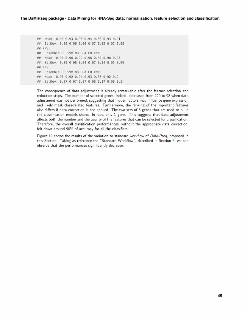
The DaMiRseq package - Data Mining for RNA-Seq data: normalization, feature selection and classification
## Mean: 0.94 0.93 0.95 0.94 0.88 0.93 0.91
## St.Dev. 0.06 0.06 0.06 0.07 0.12 0.07 0.08
## PPV:
## Ensemble RF SVM NB LDA LR kNN
## Mean: 0.98 0.96 0.99 0.96 0.88 0.98 0.93
## St.Dev. 0.05 0.08 0.04 0.07 0.14 0.05 0.09
## NPV:
## Ensemble RF SVM NB LDA LR kNN
## Mean: 0.93 0.92 0.94 0.93 0.86 0.92 0.9
## St.Dev. 0.07 0.07 0.07 0.08 0.17 0.08 0.1
The consequence of data adjustment is already remarkable after the feature selection andreduction steps. The number of selected genes, indeed, decreased from 220 to 98 when dataadjustment was not performed, suggesting that hidden factors may influence gene expressionand likely mask class-related features. Furthermore, the ranking of the important featuresalso differs if data correction is not applied. The two sets of 5 genes that are used to buildthe classification models shares, in fact, only 1 gene. This suggests that data adjustmentaffects both the number and the quality of the features that can be selected for classification.Therefore, the overall classification performances, without the appropriate data correction,felt down around 90% of accuracy for all the classifiers.Figure 19 shows the results of the variation to standard workflow of DaMiRseq, proposed inthis Section. Taking as reference the “Standard Workflow”, described in Section 3, we canobserve that the performances significantly decrease.
45

The DaMiRseq package - Data Mining for RNA-Seq data: normalization, feature selection and classification
0.6
0.7
0.8
0.9
1.0
Ensemble RF SVM NB LDA LR kNNClassifiers
Acc
urac
y
factor(Classifiers)
Ensemble
RF
SVM
NB
LDA
LR
kNN
Figure 19: Accuracies ComparisonThe violin plot shows the effect of the modification to DaMiRseq standard workflow, described in Sec-tion 6: without adjusting data (following the steps described in Section 3.4), performances usually de-crease; this could be explained by the fact that some noise, probably coming from unknown source of varia-tion, is present in the dataset.
7 Check new implementations!
7.1 Version 2.0.0, devel: 2.1.0
Since version 2.0.0 of the software, DaMiRseq offers a solution to solve two distinct problems,in supervised learning analysis: (i) finding a small set of robust features, and (ii) building themost reliable model to predict new samplesRelevant modifications:
• Since version 2.0.0 of the software, DaMiRseq offers a solution to solve two distinctproblems, in supervised learning analysis: (i) finding a small set of robust features, and(ii) building the most reliable model to predict new samples;
• The functions DaMiR.EnsembleLearning2cl_Training, EnsembleLearning2cl_Test andEnsembleLearning2cl_Predict were deprecated and replaced by DaMiR.EnsL_Train,DaMiR.EnsL_Test and DaMiR.EnsL_Predict, respectively;
• We have created a new function (DaMiR.ModelSelect) to select the best model in amachine learning analysis;
• We have created two new functions (DaMiR.iTSnorm and DaMiR.iTSadjust) to normal-ize and adjust the gene espression of independent test sets;
46

The DaMiRseq package - Data Mining for RNA-Seq data: normalization, feature selection and classification
• Two types of expression value distribution plot were added to the DaMiR.Allplot func-tion.
Minor modifications and bugs fixed:• Now, the DaMiR.FSelect function properly handles multi factorial experimental settings;• The DaMiR.FBest function cannot select less than 2 predictors, whatever the mode;• The axes labels in the RLE plot (DaMiR.Allplot function) are better oriented.
7.2 Version 1.6, devel: 1.5.2
Relevant modifications:• The DaMiR.normalization embeds also the ’logcpm’ normalization, implemented in
the edgeR package.• Now, DaMiR.EnsembleLearning calculates also the Positive Predicted Values (PPV)
and the Negative Predicted Values (NPV);• Three new functions have been implemented for the binary classification task: DaMiR.EnsembleLearning2cl_Training,
DaMiR.EnsembleLearning2cl_Test and DaMiR.EnsembleLearning2cl_Predict. The firstone allows the user to implement the training task and to select the model with thehighest accuracy or the average accuracy; the second function allows the user to testthe selected classification model on a test set defined by the user; the last functionallows the user to predict the class of new samples.
Minor modifications and bugs fixed:• Removed black dots in the violin plots.
7.3 Version 1.4.1
• Adjusted Sensitivity and Specificity calculations.
7.4 Version 1.4
Relevant modifications:• DaMiRseq performs both binary and multi-class classification analysis;• The “Stacking” meta-learner can be composed by the user, setting the new parameter
cl_type of the DaMiR.EnsembleLearning function. Any combination up to 8 classifiers(“RF”, “NB”, “kNN”, “SVM”, “LDA”, “LR”, “NN”, “PLS”) is now allowed;
• If the dataset is imbalanced, a “Down-Sampling” strategy is automatically applied;• The DaMiR.FSelect function has the new argument, called nPlsIter, which allows the
user to have a more robust features set. In fact, several feature sets are generatedby the bve_pls function (embedded in DaMiR.FSelect), setting ’nPLSIter’ parametergreater than 1. Finally, an intersection among all the feature sets is performed to returnthose features which constantly occur in all runs. However, by default, nPlsIter = 1.
Minor modifications and bugs fixed:
47

The DaMiRseq package - Data Mining for RNA-Seq data: normalization, feature selection and classification
• DaMiR.Allplot accepts also ’matrix’ objects;• The DaMiR.normalization function estimates the dispersion, through the parameter
nFitType; as in DESeq2 package, the argument can be ’parametric’ (default), ’local’and ’mean’;
• In the DaMiR.normalization function, the gene filtering is disabled if minCount = 0;• In the DaMiR.EnsembleLearning function, the method for implementing the Logistic
Regression has been changed to allow multi-class comparisons; instead of the native lm
function, the bayesglm method implemented in the caret train function is now used;• The new parameter second.var of the DaMiR.SV function, allows the user to take into
account a secondary variable of interest (factorial or numerical) that the user does notwish to correct for, during the sv identification.
8 Session Info
• R version 4.0.0 (2020-04-24), x86_64-pc-linux-gnu• Locale: LC_CTYPE=en_US.UTF-8, LC_NUMERIC=C, LC_TIME=en_US.UTF-8, LC_COLLATE=C,
LC_MONETARY=en_US.UTF-8, LC_MESSAGES=en_US.UTF-8, LC_PAPER=en_US.UTF-8,LC_NAME=en_US.UTF-8, LC_ADDRESS=en_US.UTF-8, LC_TELEPHONE=en_US.UTF-8,LC_MEASUREMENT=en_US.UTF-8, LC_IDENTIFICATION=en_US.UTF-8
• Running under: Ubuntu 18.04.4 LTS
• Matrix products: default• BLAS: /home/biocbuild/bbs-3.11-bioc/R/lib/libRblas.so• LAPACK: /home/biocbuild/bbs-3.11-bioc/R/lib/libRlapack.so• Base packages: base, datasets, grDevices, graphics, methods, parallel, stats, stats4,
utils• Other packages: Biobase 2.48.0, BiocGenerics 0.34.0, DaMiRseq 2.0.0,
DelayedArray 0.14.0, GenomeInfoDb 1.24.0, GenomicRanges 1.40.0, IRanges 2.22.0,S4Vectors 0.26.0, SummarizedExperiment 1.18.0, caret 6.0-86, ggplot2 3.3.0,knitr 1.28, lattice 0.20-41, matrixStats 0.56.0
• Loaded via a namespace (and not attached): AnnotationDbi 1.50.0,BiocFileCache 1.12.0, BiocManager 1.30.10, BiocParallel 1.22.0, BiocStyle 2.16.0,Biostrings 2.56.0, DBI 1.1.0, DESeq 1.40.0, DESeq2 1.28.0, EDASeq 2.22.0,FSelector 0.31, FactoMineR 2.3, Formula 1.2-3, GenomeInfoDbData 1.2.3,GenomicAlignments 1.24.0, GenomicFeatures 1.40.0, Hmisc 4.4-0, MASS 7.3-51.6,MSQC 1.0.2, Matrix 1.2-18, ModelMetrics 1.2.2.2, R.methodsS3 1.8.0, R.oo 1.23.0,R.utils 2.9.2, R6 2.4.1, RColorBrewer 1.1-2, RCurl 1.98-1.2, RSNNS 0.4-12,RSQLite 2.2.0, RWeka 0.4-42, RWekajars 3.9.3-2, Rcpp 1.0.4.6, Rsamtools 2.4.0,ShortRead 1.46.0, XML 3.99-0.3, XVector 0.28.0, abind 1.4-5, acepack 1.4.1,annotate 1.66.0, arm 1.11-1, aroma.light 3.18.0, askpass 1.1, assertthat 0.2.1,backports 1.1.6, base64enc 0.1-3, bdsmatrix 1.3-4, biomaRt 2.44.0, bit 1.1-15.2,bit64 0.9-7, bitops 1.0-6, blob 1.2.1, boot 1.3-25, checkmate 2.0.0, class 7.3-17,cluster 2.1.0, coda 0.19-3, codetools 0.2-16, colorspace 1.4-1, compiler 4.0.0,corrplot 0.84, crayon 1.3.4, crosstalk 1.1.0.1, curl 4.3, data.table 1.12.8, dbplyr 1.4.3,digest 0.6.25, dplyr 0.8.5, e1071 1.7-3, edgeR 3.30.0, ellipsis 0.3.0, entropy 1.2.1,
48

The DaMiRseq package - Data Mining for RNA-Seq data: normalization, feature selection and classification
evaluate 0.14, farver 2.0.3, fastmap 1.0.1, flashClust 1.01-2, foreach 1.5.0,foreign 0.8-79, genalg 0.2.0, genefilter 1.70.0, geneplotter 1.66.0, generics 0.0.2,ggrepel 0.8.2, glue 1.4.0, gower 0.2.1, grid 4.0.0, gridExtra 2.3, gtable 0.3.0,highr 0.8, hms 0.5.3, htmlTable 1.13.3, htmltools 0.4.0, htmlwidgets 1.5.1,httpuv 1.5.2, httr 1.4.1, hwriter 1.3.2, igraph 1.2.5, ineq 0.2-13, ipred 0.9-9,iterators 1.0.12, jpeg 0.1-8.1, jsonlite 1.6.1, kknn 1.3.1, labeling 0.3, later 1.0.0,latticeExtra 0.6-29, lava 1.6.7, leaps 3.1, lifecycle 0.2.0, limma 3.44.0, lme4 1.1-23,locfit 1.5-9.4, lubridate 1.7.8, magrittr 1.5, manipulateWidget 0.10.1, memoise 1.1.0,mgcv 1.8-31, mime 0.9, miniUI 0.1.1.1, minqa 1.2.4, munsell 0.5.0, mvtnorm 1.1-0,nlme 3.1-147, nloptr 1.2.2.1, nnet 7.3-14, openssl 1.4.1, pROC 1.16.2,pheatmap 1.0.12, pillar 1.4.3, pkgconfig 2.0.3, pls 2.7-2, plsVarSel 0.9.6, plyr 1.8.6,png 0.1-7, praznik 8.0.0, prettyunits 1.1.1, prodlim 2019.11.13, progress 1.2.2,promises 1.1.0, purrr 0.3.4, rJava 0.9-12, randomForest 4.6-14, rappdirs 0.3.1,recipes 0.1.10, reshape2 1.4.4, rgl 0.100.54, rlang 0.4.5, rmarkdown 2.1, rpart 4.1-15,rstudioapi 0.11, rtracklayer 1.48.0, scales 1.1.0, scatterplot3d 0.3-41, shiny 1.4.0.2,splines 4.0.0, statmod 1.4.34, stringi 1.4.6, stringr 1.4.0, survival 3.1-12, sva 3.36.0,tibble 3.0.1, tidyselect 1.0.0, timeDate 3043.102, tools 4.0.0, vctrs 0.2.4,webshot 0.5.2, withr 2.2.0, xfun 0.13, xtable 1.8-4, yaml 2.2.1, zlibbioc 1.34.0
References
[1] Jeffrey T Leek and John D Storey. Capturing heterogeneity in gene expression studiesby surrogate variable analysis. PLoS Genet, 3(9):e161, 2007.
[2] Andrew E Jaffe, Thomas Hyde, Joel Kleinman, Daniel R Weinbergern, Joshua GChenoweth, Ronald D McKay, Jeffrey T Leek, and Carlo Colantuoni. Practical impactsof genomic data "cleaning" on biological discovery using surrogate variable analysis.BMC bioinformatics, 16(1):1, 2015.
[3] Isabelle Guyon and André Elisseeff. An introduction to variable and feature selection.Journal of machine learning research, 3(Mar):1157–1182, 2003.
[4] Yvan Saeys, Iñaki Inza, and Pedro Larrañaga. A review of feature selection techniquesin bioinformatics. bioinformatics, 23(19):2507–2517, 2007.
[5] Jerome Friedman, Trevor Hastie, and Robert Tibshirani. The elements of statisticallearning, volume 1. Springer series in statistics Springer, Berlin, 2001.
[6] Robi Polikar. Ensemble based systems in decision making. IEEE Circuits and systemsmagazine, 6(3):21–45, 2006.
[7] David H Wolpert. Stacked generalization. Neural networks, 5(2):241–259, 1992.[8] Lior Rokach. Ensemble-based classifiers. Artificial Intelligence Review, 33(1-2):1–39,
2010.[9] GTEx Consortium et al. The genotype-tissue expression (gtex) pilot analysis:
Multitissue gene regulation in humans. Science, 348(6235):648–660, 2015.[10] Martin Morgan, Valerie Obenchain, Jim Hester, and Herve Pages.
SummarizedExperiment: SummarizedExperiment container, 2016. R package version1.4.0.
[11] Michael I Love, Wolfgang Huber, and Simon Anders. Moderated estimation of foldchange and dispersion for rna-seq data with deseq2. Genome biology, 15(12):1, 2014.
49

The DaMiRseq package - Data Mining for RNA-Seq data: normalization, feature selection and classification
[12] Mattia Chiesa, Gualtiero I Colombo, and Luca Piacentini. Damirseq—anr/bioconductor package for data mining of rna-seq data: normalization, featureselection and classification. Bioinformatics, 34(8):1416–1418, 2018.
[13] Jeffrey T Leek, W Evan Johnson, Hilary S Parker, Andrew E Jaffe, and John D Storey.The sva package for removing batch effects and other unwanted variation inhigh-throughput experiments. Bioinformatics, 28(6):882–883, 2012.
[14] Matthew E Ritchie, Belinda Phipson, Di Wu, Yifang Hu, Charity W Law, Wei Shi, andGordon K Smyth. limma powers differential expression analyses for rna-sequencing andmicroarray studies. Nucleic acids research, page gkv007, 2015.
[15] Luca Piacentini, José Pablo Werba, Elisa Bono, Claudio Saccu, Elena Tremoli, RitaSpirito, and Gualtiero Ivanoe Colombo. Genome-wide expression profiling unveilsautoimmune response signatures in the perivascular adipose tissue of abdominal aorticaneurysm. Arteriosclerosis, thrombosis, and vascular biology, 39(2):237–249, 2019.
[16] Hadley Wickham. ggplot2: elegant graphics for data analysis. Springer, 2016.[17] Davide Risso, Katja Schwartz, Gavin Sherlock, and Sandrine Dudoit. Gc-content
normalization for rna-seq data. BMC bioinformatics, 12(1):480, 2011.[18] Tahir Mehmood, Kristian Hovde Liland, Lars Snipen, and Solve Sæbø. A review of
variable selection methods in partial least squares regression. Chemometrics andIntelligent Laboratory Systems, 118:62–69, 2012.
[19] Ildiko E Frank. Intermediate least squares regression method. Chemometrics andIntelligent Laboratory Systems, 1(3):233–242, 1987.
[20] Igor Kononenko. Estimating attributes: analysis and extensions of relief. In Europeanconference on machine learning, pages 171–182. Springer, 1994.
[21] Marko Robnik-Šikonja and Igor Kononenko. An adaptation of relief for attributeestimation in regression. In Machine Learning: Proceedings of the FourteenthInternational Conference (ICML’97), pages 296–304, 1997.
[22] Daniel M Cornforth, Justine L Dees, Carolyn B Ibberson, Holly K Huse, Inger HMathiesen, Klaus Kirketerp-Møller, Randy D Wolcott, Kendra P Rumbaugh, ThomasBjarnsholt, and Marvin Whiteley. Pseudomonas aeruginosa transcriptome duringhuman infection. Proceedings of the National Academy of Sciences,115(22):E5125–E5134, 2018.
[23] N. Littlestone and M.K. Warmuth. The weighted majority algorithm. Information andComputation, 108(2):212 – 261, 1994. URL:http://www.sciencedirect.com/science/article/pii/S0890540184710091,doi:http://dx.doi.org/10.1006/inco.1994.1009.
50