The Cyclical Behavior of Job Creation and Job Destruction

Econ. Theory 7,95-112 (1996) j-i

Economic Theory

? Springer-Verlag 1996

The cyclical behavior of job creation and job destruction: A sectoral model*

Jeremy Greenwood1, Glenn M. MacDonald2, and Guang-Jia Zhang3 1

Department of Economics, University of Rochester, NY 14627-0156, USA 2

W.E. Simon Graduate School of Business Administration and Department of Economics, University of Rochester, NY 14627-0156, USA

3 Department of Economics, University of Rochester, NY 14627-0156, USA, and Department of

Economics, University of Guelph, Guelph NIG 2W1, CANADA

Received: March 20,1994; revised version September 12,1994

Summary. Three key features of the employment process in the U.S. economy are

that job creation is procyclical, job destruction is countercyclical, and job creation is

less volatile than job destruction. These features are also found at the sectoral (goods and services) level. The paper develops, calibrates and simulates a two-sector general

equilibrium model that includes both aggregate and sectoral shocks. The behavior

of the model economy mimics the job creation and destruction facts. A non

negligible amount of unemployment arises due to the presence of aggregate and

sectoral shocks.

1. Introduction

What determines the amount of employment in an economy and its distribution

across sectors, or the size of the labor market and its breakdown between those with

and without jobs. In U.S. economy job creation is procyclical, job destruction is

countercyclical, and job creation is less volatile than job destruction. In a well

known paper, Lilien [10] advanced the hypothesis that variations in sectoral

opportunities together with frictions impeding the inter-sector movement of

workers play an important role in determining labor market aggregates, and in

particular unemployment. The questions raised by these findings are: Can a multi

sector dynamic general equilibrium model replicate the pattern of job creation, and

destruction that is observed in the U.S. data? Are sectoral shocks important for

determining the average rate of unemployment? The analysis seeks to explain movements in labor market aggregates as the

outcome of the interaction of aggregate and sectoral shocks. The model developed to do this is a multi-sector dynamic competitive general equilibrium framework. The

model has three key features. First, each market sector gets hit by both aggregate

* We thank Jeffrey Campbell, Richard Rogerson and two referees for helpful comments. We are grateful

to M.J.D. Powell for providing us with his GETMIN FORTRAN subroutine.

Correspondence to: J. Greenwood

96 J. Greenwood et al.

and sectoral shocks. This is similar, in spirit, to the classic Long and Plosser [12] real

business cycle model. Second, it takes time to reallocate labor across sectors. Each

sector in the market economy can draw new employees from a pool of unemployed workers seeking a job. This pool is made up of agents who entered it in some earlier

period, either because they lost their job in a market sector or left the home sector.

This feature of the analysis requiring a time cost for job reallocation bears some

resemblance to the well-known Lucas and Prescott [14] equilibrium search model.

Third, following Hansen [6] and Rogerson [20], it is assumed that labor is

indivisible. This assumption ensures that the options of working, searching and

staying at home are mutually exclusive.

The model developed reproduces the cyclical pattern of job creation, destruction

and reallocation displayed in the U.S. data relatively well. Workers flow between

sectors as jobs are created and destroyed in response to both aggregate and

sector-specific shocks. A conclusion of the paper is that aggregate and sectoral

shocks contribute a non-negligible amount to the average level of unemployment.1 Here, approximately one percentage point of the unemployment rate can be

accounted for by aggregate and sectoral shocks. The fact that generally some

workers are unemployed, but ready to work, allows sectors to expand their output more rapidly in reaction to favorable circumstances in much the same way as

inventories of raw materials, parts, etc. do.2

The rest of the paper sets out the model in detail and explores its features

quantitatively.

2. Model

The multisector dynamic general equilibrium model to be simulated will now be

developed.

2.1 Economic environment

A continuum of ex ante identical agents is distributed uniformly over the unit

interval. In period t an agent can work in one of two productive sectors, search for a job, or stay at home. To describe this, let nit represent the fraction of agents who are working in sector i at i, and n3a denote the fraction of agents who are searching. Thus, the fraction of the population currently at home is 1 ?

?f= x nit while

1 ? X!2= 17r?,f is the proportion not working. A description of tastes, technology and

the stochastic structure of the model follows.

2.1.1 Tastes Let cit represent an agent's period-i consumption of the commodity

produced in sector i. An agent has one unit of non-sleeping time. Labor effort is

indivisible with it being assumed that work and search require w and s hours of

effort, respectively. Leisure is then given by 1 ? lt9 where lte{0,s,w}. An agent's

1 Andolfatto [1] studies the equilibrium determination of unemployment within the context of a match

ing model (that has both aggregate and idiosyncratic shocks). 2

Clearly technological advances, such as changes in organizational forms, that allow inputs to be

allocated more quickly to their end-uses are likely to be desirable.

Job creation and destruction 97

expected lifetime utility is given by

e\ ? ?F | A In i eiCUlt)JP

+ (1 - A)\n(l - /,)jl

(1) where ?e(091), pe(- oo,0)u(0, l],0?e(O, 1), and ??=1 0f

= l.3

2.1.2 Production technology Sector i is subject to both aggregate, zt9 and sectoral,

sit9 disturbances. There is a firm in each sector i that produces output yit according to

the production technology:

yut =

î?Kî-?i^tî,tl (2) where

ht =

wK? -

y?(maxl>.\? -

*,-,,-i,0])Ai]. (3)

In (2) /i,-, represents the amount of labor input hired by the firm. Hiring new labor is

costly. One of the costs is assimilating new workers into the production process, a feature portrayed by (3). This cost is increasing in the number of workers that join the firm. This is equivalent to saying that when new workers are hired in a period

they are less productive than experienced workers. The term /?(z,, eit) is an output

reducing shock. This function is discussed in more detail below. By substituting (3) into (2) it is easy to see that production is governed by

yut =

ztsutwaiiî,t -

yi(max[7ciff -

nUt.?OW -

It(zpeUt). (4)

Firms are owned by households.

2.1.3 Search technology In order to increase its employment a firm must draw new

labor from the search pool. Thus, the increase in employment that can occur in a sector is limited by the size of the existing search pool. Specifically,

2

? max{0,7?i>? + 1-7c?ff}<7c3fr (5) ? = i

Note that (5) implies any reallocation of agents between sectors l and 2 will involve a one period transition cost.

2.1.4 Stochastic structure The aggregate and sectoral disturbances are independent of one another and follow finite-state first-order Markov processes with supports Z =

{z19z29...9zm} and Et =

{s?9...9s }9 respectively. Furthermore, it will be as

sumed that the shocks in sectors l and 2 are inversely related to one another. In

particular, let ex =

l/e2 = e.

2.2 Planner's problem

Following Rogerson [20] and Hansen [6] the representative household's choice set

is extended to include the possibility of a lottery over their consumption and labor

allocations. One can think about the lottery mechanism as an employment contract

3 The case where p

= 0 is easily handled by letting the expected value of lifetime ulitity read


specifying for each /e{0, s, w} sl (state-contingent) probability n(l) that the agent will

work / hours, consume ct(l) units of sector-i output and enjoy 1 - / units of leisure.

Since all agents are alike initially, it follows from using an appropriate law of large numbers that 7c(0)

= 1 ? ??= x ni9 n(s)

= n3, and 7c(w)

= ?,2= x 7i?. The planner's dy

namic programming problem that determines the form of this contract is shown

below.

V(Kz,e) = maxMn)MM ?-Y n?]\-\n( Y 0fcf(O) (n;z,e) =

max{ci(I)?i{<)| ? 1 - ? n'A -In? ? 0,-c?

Jln(?0,<(s)W-?)ln(l-s)l 4 P

+ i?; ln(? e^w)) + (l-?)-ln(l-w)l

subject to

+ ?EiV(n';z',s!)\n;z,{\

1 - ? ?jW) + ( ? ?iVi(w) + ̂ c,(s)

P(l)

= Z??Wai 7T?. y^maxCTcJ-TcÔ])^

3

/?(z,^), for i =1,2,

? max {0,7rJ

? 7iJ < 7r3,

(6)

(7)

(8)

(9) 7t;>0, for i =1,2,3.

The resource constraint for each sector is given by (6). The next constraint limits the

aggregate amount of labor that can be used in non-leisure activities. Equation (8) states that the amount of new labor that can be hired by sectors 1 and 2 is restricted

by the size of the search pool. Given the separability of preferences, the planner will select consumption paths

that are independent of agents' labor market status.4 Thus, P(l) can be simplified to

V(n;z,e) = max{??}

j^ln I" ? 0,(ze, **[*;

- y,(max [>',

- nt,0])*']*

- ?,(z,et)Y 1

- A)L?3ln(l

- s) + ( ? ;An(l

- w) + (1

+ ?-E\_V(n';z',e')\n;z,?-]

subject to (7), (8), and (9).

P(2)

4 For more detail, see Greenwood and Huffman [5] or Rogerson and Wright [21].


SECTOR 1: Goods

Construction Mining Manufacturing

[Transp. & Pub. Utilities Wholesale & Retail Trade

SECTOR 2 : Services

Finance, Insurance & Real Estate

Figure 1.

2.3 Discussion

Multisector frameworks similar to the one presented above have been developed in

Rogerson [19] and Hornstein [9]. The planning problem P(l) determines a Pareto

optimal allocation for the economy under study. An interesting question that arises

is whether or not this Pareto-optimal allocation can be decentralized as a competi tive equilibrium? By extending the analysis of Prescott and Rios-Rull [17], it should

be possible to show that this allocation can be supported as a quasi-competitive

equilibrium. A key step in doing this is to represent the commodity space as a set of

infinite sequences of measures specifying the odds of consuming a given quantity of

goods and leisure, contingent upon a particular history of aggregate and sectoral

shocks.

3. Calibration

The model is restricted to two sectors, assumed to correspond to the goods and

service sectors of the U.S. economy. The industries that make up these sectors are

shown in Figure 1; one period is assumed to be one quarter.

3.1 Preference parameters

The quarterly interest rate is taken to be one percent; thus the discount factor, ?9 is

0.99. Next, data from the Monthly Labor Review shows that, on average, the

employed work 39 out of the approximately 100 non-sleeping hours per week

available to them; consequently, w = .39. According to Barron and Mellow [2], the

mean number of hours spent searching per week is approximately 7 which implies s = .07. In a similar vein, a value of 0.28 was picked for the coefficient A in the utility function. This results in approximately 25% of aggregate non-sleeping hours being


spent at work. In the U.S. data the goods sector is about 58 percent of the size of the

service sector, when measured by employment. This occurs in the model's steady state if 0X

= .43 (92 =

.57). Finally, the parameter pe(? oo, 1] governs the amount of

substitution between goods and services in the utility function. Independent evi

dence on an appropriate value for p is hard to come by. In the subsequent analysis, p is assigned a value of 0.55.5

3.2 Technology parameters

The two production function parameters, a1 and a2, are set equal to 0.74 and 0.64

respectively. These numbers are labor's share of income in goods and services

sectors for the 1964-1987 period.6

3.3 Adjustment costs

The adjustment cost parameters, Xt and yi9 are set at 2.0 and 5.5, respectively, for both

sectors. These are free parameters that determine the speed of sectoral employment

adjustment.7

3.4 Shocks

Recall the assumption that et =

l/e2 = ? - this amounts to assuming a single relative

sectoral shock. Then, using (2) and data for each sector's output and labor input, the

aggregate and sectoral Solow residuals are easy to calculate.8 By doing this it is

found that the aggregate shock has a percentage standard deviation of 0.04 and a serial correlation coefficient of 0.93. The numbers for the sectoral shock are 0.015

and 0.93.

The aggregate and sectoral shocks are two-state Markov processes:

zteZ =

{expêxp-^} with Pr[z' =

z1|z =

z1] =

Pr[z' =

z2|z =

z2], and seE =

{expc,exp"c} with Pr[e' =

e1|? =

?i] =

Pr[e' =

?2\e =

?2]- The parameters ? and

5 The utility function specified in ( 1) implies that an agent will divide his consumption between goods and

Ci 1 services according to the formula In?=-lnp, where p is the relative price of goods in terms of

c2 p-1 services. Estimation of this equation using instrumental variables yielded a value of .55 for p. Unfortu

nately, this point estimate was insignificant at the 95% level of confidence. Still, on the basis of the time

series evidence a value of 0.55 is the best guess for p. 6

Labor's share of income for sector i, or a? was computed from the formula shown below using data from

the National Income and Product Accounts:

COMt a'~

Nli + CCAi-Pl/

where COMt is Compensation of Employees for sector i, NI? is National Income, CCA? is the Capital

Consumption Allowance, and P/? is Proprietor's Income. 7

The adjustment costs are quantitatively trivial in magnitude. The loss in labor input due to adjustment costs averages less than 0.0028 percent of total employment in the simulations undertaken. 8

The assumption on the functional form for the sectoral disturbances allows them to be easily identified.


C are chosen so that the time series properties for the aggregate and sectoral

disturbances in the model inherit the time series behavior of the aggregate and

sectoral Solow residuals. This implies setting ? = .04, Pr[z'

= z1|z

= z1]

= .965,

C = .015 and Pr[e'

= ex\s

= ?J

= .965.9

3.5 Investment

Finally, in the U.S. economy consumption is relatively smooth, and investment is

procyclical and highly volatile. This motivates subtracting a certain amount of

output, equal to investment, from the right hand side of the resource constraints.10 The function It(z9 et) is intended to capture this. Let the investment functions, It(z9 et)9 have the form

fea+<TiIf9 if z = ??* and et =

^9

I ea~aiIf9 if z = e* and et =

e~^9 i?(z'??)

"

] e-'

+ ?I*9 if z = e~? and et

= e\

[e~a~aiIf9 if z = e~t and ??

= e~c,

where the means and standard deviations of ln/^z^) are given by ln/f and

In the U.S., aggregate investment is approximately 20 percent of GNP. This

implies that in the model's steady state Ix + pl2 =

2\^yi + py2], where p is the rela

tive price of good two. Also, the goods producing sector generates two-thirds as

much output as the service sector. If it is assumed that investment spending is spread across sectors proportionally, then the model's steady state should display the

feature that IJI2 =

yjy2. Assuming this, along with Jx + pl2 =

.2\_yi + py2\ im

plies I\ = .0378 and /* = 0605. In the U.S. data, investment is four times as volatile

as output and the correlation coefficient between aggregate investment and output is 0.95. The percentage standard deviations for the investments were chosen to

mimic these observed facts. This involved setting o = .08, o1 = .06, and o2

? .08.

4. Findings

The cyclical properties of the above model are developed through simulation. As is now standard, the procedure is to compare a set of stylized facts characterizing the

business cycle behavior of the model with a analogous set describing U.S. postwar business cycle behavior over the 1964.1-1987.4 sample period. Appendix A details

the computational procedure used to calculate the decision-rules associated with the

planner's problem. The procedure used to compute the decision-rules is complicated

by the presence of the inequality constraint (8). With these decision-rules in hand,

9 It is straightforward to calculate that the percentage standard deviations of the aggregate and sectoral

disturbances are given by ? and ?. Likewise, the formulae for the autocorrelation coefficients for the

shocks are 2 Pr[z' =

zx \z =

zj ? 1 and 2 Pr[e'

= ?1 |e

= aj

? 1, respectively.

1 ? The aggregate disturbance will not affect the solution to the model if there is no investment term in the

resource constraint (6). This is immediate from problem P(2). Without the 7f(z, et) term, it is easy to see that

z can be factored out of the first term on the righthand side of P(2). Hence it can't affect the maximization.


Employment - Sector 1 Search Pool

Time Time

Employment - Sector 2 Nonemployment

Time

Figure 2.

Time

200 samples of 96 observations (the number of quarters in the U.S. sample period) are simulated. Each simulation run corresponds to a randomly generated sample of

96 realizations of the z and s processes. The data from the simulations is logged

(where applicable) and H-P filtered, as is the data for the U.S. economy, and average moments over the 200 samples are computed for each variable of interest.

4.1 Impulse-response functions

The dynamic effects that aggregate and sectoral disturbances have on sectoral

employment and aggregate nonemployment can be represented in terms of impulse response functions.

** This is done by fitting a first-order vector autoregression of the

form n' = c + bn + v to the simulated data, where n = [nl9 n29 7r3]T, c and b are 3x1

and 3x3 parameter vectors, and v is a 3 x 1 vector of approximation errors. Figure 2 plots the impulse response functions associated with an aggregate shock, where the

economy is assumed to be in a steady state initially. Employment in both sectors

rises, while aggregate nonemployment (or 1 ? nl

? n2) falls. Notice that it takes the

economy five periods to move agents out of the searching pool and home sector into

work in the two market sectors. This illustrates the influence of adding the search

To be nonemployed is defined here as not working. In the model the number of agents who are

nonemployed is 1 ? n^ . This is an exact concept and does not match up precisely with the notion of

being unemployed. In the U.S. data an agent is counted as being unemployed if he is not working, but has

looked for a job within the last four weeks.


Employment - Sector 1 Search Pool

Time Time

Employment -- Sector 2 Nonemployment

Time

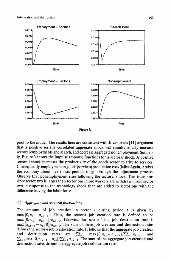
Figure 3.

Time

pool to the model. The results here are consistent with Jovanovic's [11] argument that a positive serially correlated aggregate shock will simultaneously increase sectoral employments and search, and decrease aggregate nonemployment. Similar

ly, Figure 3 shows the impulse response functions for a sectoral shock. A positive sectoral shock increases the productivity of the goods sector relative to services.

Consequently, employment in goods (services) production rises (falls). Again, it takes the economy about five to six periods to go through the adjustment process.

Observe that nonemployment rises following the sectoral shock. This transpires since sector two is larger than sector one; more workers are withdrawn from sector two in response to the technology shock than are added to sector one with the difference leaving the labor force.

4.2. Aggregate and sectoral fluctuations

The amount of job creation in sector i during period t is given by max {0,7^,? nit_x}. Thus, the sector-i job creation rate is defined to be

max{09nu ?

7iUt_1}lnit_1. Likewise, for sector-i the job destruction rate is

msLx{nUt_1 ?

î,v^}/ni,t-v The sum of these job creation and destruction rates

defines the sector-i job reallocation rate. It follows that the aggregate job creation and destruction rates are ??= x max {0, nUt

? nUt _ x }/??= x nUt _ x and

1?f=imsix{097ti^1 -nitt}fZ?=i Ht-i- The sum of the aggregate job creation and destruction rates defines the aggregate job reallocation rate.


Table 1. Cyclical behavior of U.S. labor market aggregates (Quarterly, 1964.1?

1987.4)

Variables S.D. (%) Corr/Output Corr/Employment

Output 2.50 1.00 0.86

Employment 1.66 0.86 1.00

Hours 1.96 0.91 0.98

Nonemployment - 0.93 - 0.92

Job creation rate 0.71 0.46 0.12

Job destruction rate 1.82 -0.47 -0.20

Job reallocation rate 0.56 -0.14 -0.12

Productivity 1.06 0.66 0.20

Note: The U.S. economy analyzed in this paper consists of two sectors. One of

them, Sector 1, is the Goods sector which includes three 1-digit SIQ1987)

industries: Mining, Construction, and Manufacturing. The other, Sector 2, is

the Service sector which includes the following SIC industries: Transportation and Public Utilities, Wholesale Trade and Retail Trade, Finance-Insurance and

Real Estate, and Services. All industry time series are taken from CITIBASE

(1989). Since quarterly GNP by industry is not available, National Income is

used as substitute. The availability of data on average weekly hours worked by

industry determines the sample periods starting from 1964.1 to 1987.4. For

productivity, Corr/Employment represents the correlation of productivity and

hours. All series are logged (where applicable) and detrended using the

Hodrick-Prescott filter.

Table 2. Cyclical behavior of labor market aggregates (Model: 200 simulations

with 96 observations each)

Variables S.D. (%) Corr/Output Corr/Employment

Output 1.92 1.00 0.87

Employment 0.29 0.87 1.00

Hours 0.29 0.87 0.99

Nonemployment ?0.87 ?1.00

Job creation rate 1.69 0.26 0.03

Job destruction rate 1.95 -0.30 -0.22

Job reallocation rate 1.54 -0.04 -0.12

Productivity 1.67 0.99 0.81

Note: All time series are logged (where applicable) and detrended using the H-P

filter. The statistics shown in all tables are the average values after 200

simulations of 96 observations each. For productivity, Corr/Employment

represents the correlation of productivity and hours.

Descriptive statistics characterizing the cyclical behavior of U.S. labor market

aggregates are presented in Table 1. Table 2 presents the same statistics for the

model. The model reproduces the cyclical pattern of job creation, destruction and

reallocation displayed in the U.S. data relatively accurately. Specifically,

In both the model and the data, the job creation rate moves procyclically while

the job destruction and reallocation rates are countercyclical. The c?rrela


tions between these variables, on the one hand, and GNP and employment, on

the other, are also close to those found in U.S. data.

In both the model and the data the job destruction rate is more volatile than

either the job creation or reallocation rates. This reflects the importance of the

asymmetric nature of the employment process. It is much easier to fire people than to hire them.

In the data the correlation between hours and productivity is low, as

evidenced by the correlation coefficient of 0.20. For the model the number is

0.81, which is too high. On this dimension the model performs more or less the same as the standard model with indivisible labor, but worse than models that

include government spending or household production - see Hansen and

Wright [8]. Another shortcoming is that hours worked in the model is much

less volatile than in the data. Consequently, productivity fluctuates more in

the model than in the data. This is due to the presence of adjustment costs for

hiring labor.12

Next, some stylized facts describing the behavior of U.S. labor market variables

at the sector level are given in Table 3. Table 4 presents the same set of facts for the

model. The key findings here are:

In the data, the job creation, destruction and reallocation rates display the

same pattern of cyclical behavior at the sectoral level as they do for the

economy as a whole. There is, however, one exception: while the job realloca

tion moves countercyclical^ in the goods producing sector it moves procycli

cally in services.13 The model replicates fairly closely the correlation structure

between these variables and output, except for the procyclical movement of

the job reallocation rate in the service sector.

The model and data share the feature that output and employment are more

volatile in goods production than in services.

The model does a much better job matching the hours/productivity correla

tions observed at the sectoral level.

Finally, Table 5 reports negative correlations between job creation and destruc

tion rates, at both the aggregate and sectoral levels. Similar findings are reported in

Mortensen [15]. On this,

The model yields mixed results here. On the one hand, a positive correlation

between aggregate job creation and destruction is displayed by the model. On

the other, the model does replicate the negative association between job

12 Hours fluctuates more than productivity in the data. Hansen [6] matched this fact by introducing

indivisible labor into an otherwise standard stochastic growth model. In the current analysis productivity is more volatile than hours, notwithstanding the use of indivisible labor. 13

The size of the service sector has increased over time while the volume of goods production has

declined. Jobs created in the service sector may accelerate during booms and jobs destroyed in the goods sector may speed up in recessions. This hypothesis is consistent with findings in Loungani and Rogerson

[13].


Table 3. Cyclical behavior of sector labor aggregates in U.S. economy (Quarterly, 1964.1-1987.4)

Variables S.D. (%) Corr with Output Corr with Employment

Sector 1 Sector 2 Sector 1 Sector 2 Sector 1 Sector 2

Output 4.12 1.50 1.00 1.00 0.87 0.77

Employment 2.94 1.00 0.88 0.77 1.00 1.00

Hours 3.50 1.02 0.93 0.81 0.98 0.98

Job creation rate 1.31 0.56 0.32 0.47 0.03 0.14

Job destruction rate 1.68 2.95 -0.49 -0.40 -0.24 -0.16

Job reallocation rate 0.96 0.47 -0.37 0.31 -0.24 0.07

Productivity 1.54 0.90 0.56 0.75 0.12 0.18

Note: For productivity, Corr/Employment represents the correlation of productivity and hours.

Table 4. Cyclical behavior of sector labor aggregates (Model: 200 simulations with 96 observations each)

Variables S.D. (%) Corr with Output Corr with Employment

Sector 1 Sector 2 Sector 1 Sector 2 Sector 1 Sector 2

Output 2.24 2.16 1.00 1.00 0.76 0.75

Employment 0.68 0.63 0.76 0.75 1.00 1.00

Hours 0.68 0.63 0.76 0.75 1.00 1.00

Job creation rate 2.65 2.15 0.30 0.37 0.10 0.18

Job destruction rate 2.97 2.32 -0.37 -0.38 -0.22 -0.19

Job reallocation rate 1.85 1.44 -0.08 -0.02 -0.10 0.00

Productivity 1.77 1.74 0.95 0.96 0.57 0.57

Table 5. Relation between job creation and destruction (Correlation)

Aggregate Sector 1 Sector 2

U.S. data

(Quarterly, 1964.1-1987.4) -0.50 -0.37 -0.44

Model

(200 simulations) 0.40 -0.13 -0.18

creation and destruction observed at the sectoral level, although it understates the size of the correlations.

4.3 The determination of aggregate unemployment

How much of unemployment can be accounted for by aggregate and sectoral

shocks? In the absence of technology shocks there would be no steady-state search

unemployment in the model. Thus, the average value for n3 is a measure of the


amount of unemployment due to aggregate and sectoral disturbances.14 On this

account 1.20 percent of the labor force is unemployed. To get a rough estimate of

how the aggregate and sectoral shocks contribute to unemployment, the aggregate and sectoral shocks can be shut down in turn. When the aggregate shock is shut

down (i.e., ? = 0 and (

= .015) the average value for n3 falls to 0.97. The average value

of 7i3 drops to 1.00 when the sectoral shock is turned off (i.e., ? = 0.04 and ?

= 0).

Thus, aggregate and sectoral shocks have a similar effect on the average level

unemployment. Finally, the procyclical nature of quits in the U.S. economy suggests that job search is procyclical (see Jovanovic [11]). The model predicts that the

search is procyclical, that is the correlation between n3 and output is 0.61.

4.4 Discussion

The job creation and destruction rates computed above represent the lower bounds on the amount of job creation and destruction in the U.S. economy. To ease the

burden of the quantitative analysis the economy was dichotomized into two broad

sectors, goods and services. If the economy was disaggregated down further into

many sectors the amount of job creation and destruction would increase.15 In fact, the amount of job creation, destruction, and reallocation could be disaggregated

down to the level of the plant, as Davis and Haltiwanger [4] do for the manufactur

ing sector of the U.S. economy. They find that job creation is procyclical, job destruction is countercyclical, and the latter is more volatile than the former. In

a model with many sectors, and perhaps many plants within a sector, the amount of

steady-state search unemployment due sectoral and plant-specific shocks should

increase. On this, in a study of 26 U.S. industries, Loungani and Rogerson [13] find

that approximately 5.5 percentage points of unemployment among workers can be

accounted for by industry switchers.

5. Concluding remarks

A multisector dynamic general equilibrium model is constructed here to analyze the

cyclical pattern of job creation and destruction. The two main ingredients in the

model are the Lucas-Prescott [14] idea that it takes time to find employment and

the Rogerson [20]/Hansen [6] notion of indivisible labor. It is found that the model

can successfully replicate the cyclical patterns of job creation, destruction and

reallocation that is observed at both the aggregate and sectoral levels in the U.S.

economy. Specifically, job creation rates move procyclically in the model while job destruction rates move countercyclical^, as they do in the data. Also, in the model

job destruction is more volatile than either job creation or reallocation, a feature

14 It is being assumed that all agents in the search pool would qualify as being unemployed, as measured

in the U.S. data - see footnote 11.

15 The job creation rate in an JV-sector model is given by ?f= 1 max {0, nit

? nit_ i}/ZJL x ni,t-v Now,

consider aggregating the N sectors up into 2 sectors. The rate of job creation for the aggregated 2-sector

model would be max {0,1^ (*,,,-*,,,_ 1)}/Zf=1 nitt^ +

max{0,SfssJf+1(7ritf-?,,,_JJ/Zf^ 1 tc^^.

Clearly, the latter sum is smaller than the former one.


displayed in the data. Finally, it is found that aggregate and sectoral disturbances

contribute non-negligibly to unemployment. In the model presented here workers were assigned their employment status via

a lottery. They were perfectly insured against the possibility of dismissal, in the sense

that their consumption in a period was not contingent upon their employment status. One can imagine a world where no such insurance exists. Suppose, instead, that individuals can only insure themselves by saving in the form of a simple asset, such as money or government bonds. Each period those agents currently working in

a sector decide whether to stay at work, enter the unemployment pool to search for

a new job in another sector, or leave the labor force. Agents in the unemployment

pool decide whether to take a job in some sector, remain in the unemployment pool for another period, or leave the labor force. Likewise, those individuals at home

must decide whether or not to enter the labor force. Clearly, an individual's decision

will be predicated upon both his idiosyncratic circumstance (asset holdings, employ ment status) and the aggregate situation (the distribution of agents and state of

technology in each sector). While computationally more complicated, such an

analysis would undoubtedly share many of the features of the above model. But it

would permit a much richer analysis along some dimensions. For instance, one

could study the effect that government policies, such as unemployment insurance, have on intersector mobility and unemployment.16 The current analysis can be

viewed as a first step toward such a model.

Appendix

A: Computation

Modified discrete state space approach with value function approximation The neoclassical growth model can be solved using standard discrete state space dynamic programming

techniques. In economies with multiple sectors or multiple agents, the standard approach becomes

unworkable due to the curse of dimensionality, which limits the practicability of standard discrete state

space dynamic programming techniques for large problems. An alternative treatment of the problem is to store a limited set of coefficients characterizing

a parameterized value function and momentary return function.17 The parameterized objective function

can then be maximized using an optimization routine. Two benefits derive from this method: First,

computation costs are reduced dramatically; and second, the maximizers are no longer constrained to lie

in a discrete subset of the constraint set.

An obvious candidate in the family of simple functions to use to approximate more complicated functions is the polynomial. However, there are two problems associated with polynomial approxi

mation. First, practical concerns prevent using high order polynomials (even given the Weierstrass

theorem). Second, the adequacy of polynomial approximations depends on the differentiability

properties of the function that is being approximated. Often, for a smooth function a lower degree

polynomial can be used.18

16 This policy experiment could be viewed as embedding the analysis of Hansen and Imrohoroglu [7]

into a multisector general equilibrium model of the form presented here. 17

A discussion of numerical techniques used to solve dynamic equilibrium models can be found in

Dan thine and Donaldson [3]. 18

Given the assumptions placed on tastes and technology here, the value function will be strictly

increasing, and strictly concave (Stokey et al. [22], Chap. 9).


The representative agent's optimization problem, characterized by problem P(2) in Section 2, can be

simplified to one with only linear constraints by using the following lemma. For this simplified problem, it

is easy to check the convexity of the constraint set.

Lemma 1 The transition constraint

2

? max {0, n'.

- rcj <n3 (10)

?=i

is equivalent to following set of linear inequality constraints:

7c'l+7r'2<7r1+7r2 + 7r3, (11)

n'i<ni+n3, (12)

n'2<n2 + n3. (13)

Proof: It is trivial to verify that the set constrained by (10) is same as the one constrained by (11), (12) and

(13). If (10) holds, then the following must be true,

(Wj ?

Tt!) + (7C'2

? 7T2) < JC3, (14)

n\ -

nx < tc3, (15)

7c'2 -

n2 < n3. (16)

But this is merely (11)?(13). On the other hand, from (14)?(16) it is easy to derive that

max {0, n'x ?

n^} + max {0, n'2 ?

n2} <

max{0, n3}, (17)

which is equivalent to the transition constraint (10).

Let & represent the space of continuous, bounded functions and consider the mapping T:!F^&

defined by P(3).

^+1(7c1,7r2,7r3;z,?1,e2) =

max{)ri,j:,,JtJ-ln( ? e^î^-y^m^l^-n^fT-lii^dY

2

+ (l-i4)r>r'Jln(l-s) + (l

An(l-w)l

3

+ j??[KJ(7r/l,7c2,7c/3;z',e'l,22)|7r1,7r2,7r3;z,?1,82]^,

P(3)

subject to the constraints (11)?(13) and

X <<U n[>0. (18) ; = i

The mapping T maps Vj to VJ+1. This operator is a contraction mapping that has as its unique fixed point the function V defined by P(2).19 This last observation motivates the computational procedure used here

consisting of the following steps:

1. A grid is defined over the model's state space. Specifically, it is assumed that nle[.243,.297],

7i2e[.360, .440], and 7c3e[0, .024].20 Three grids of 13 equally spaced points are layered over these

intervals. These sets of grid points are denoted by IJ^ IJ2, and 773, respectively. 2. An initial guess for the 2nd degree polynomial used to approximate the value function over this

grid is made.

19 It is trivial to check that P(3) satisfies Blackwell's sufficiency conditions for a contraction mapping

-

seeStokeyetal.(1989). 20

By simulating the model it was determined that system never left these intervals.

o

3 O a

Table 6. Codes of the time series in citibase (Sample period: 1964.1-1987.4)

Variables Industries

A: Output National income GYWM GYWC GYM GYWTU

GNP(82) GA8G14 GA8G15 GA8GM GA8GTU GNP GAG14 GAG15 GAGM GAGTU

B: Labor

Employment LPMI LPCC LPEM LPTU

Weekly hours worked LWMI6 LWCC LPHRM LWTU per employee

Unemployment rate LURMI LURC LURM LURTPU

C: Labor share

Compensation of total GAPMI GAPCC GAPM GAPTPU

employees

Proprietor's income GAYPMI GAYPCC GAYPM GAYPTU

Corporate capital GACMI GACCC GACM GACTPU

consumption allowance

GYNRR+GYNRW GYFIR GYS GA8GW + GA8GR GA8GFE GA8GS GAGW + GAGR GAGFE GAGS

LPT LPFR LPS LWTWR LWFR6 LWS

LURWR LURFS LURFS

GAPW + GAPR GAPFF GAPS

GAYPTW + GAYPRT GAYPF GAYPS GACW + GACR GACFF GACS

D: Population Civilian population P016

Note: -The industry numbers are defined in the text of Appendix B.

-All time series, except ones at annual frequency, are seasonally adjusted. -All time series in groups A and C are nominal, except GNP which is in 1982 dollars.

-All series in groups A and C are annual, except national income which is quarterly, and all series in groups B and D are monthly.


3. Given the guess for the value function, a maximization routine is used to solve the constrained

nonlinear optimization problem P(3) for the optimal decision-rules.21 This is done for each of the

8,788 points in the set nvx II2x il3x Z x E.

4. Using the solution obtained for the optimal decision-rules, a revised guess for the value function is

computed. This is done by choosing a new 2nd degree polynomial to approximate the value

function. In particular, from P(3) a value for V can be computed for each grid point in the set

IJ1 x IJ2x IJ3x Z x E. A 2nd degree polynomial is then fitted to these points via least squares. 5. The decision-rules are checked for convergence.

Once the decision-rules have been obtained, the model can be simulated and various statistics are

generated consequently. Note that function values for the decision-rules will have been computed for

each point in the set IJl x Tl2 x 773 x Z x E. It is then easy to obtain values for the decision-rules at any

point in the space [.243, .297] x [.360, .440] x [0, .024] x Z x E by using multilinear interpolation - see

Press et al. [18]. The adequacy of using a 2nd degree polynomial to approximate the value function can

be assessed from a R2 statistic. The R2 obtained from using the 2nd degree polynomial was 0.96.

Additionally, one could fit a higher order polynomial to the values of V obtained in the grid. Using some

appropriate metric, the distance between this polynomial and the 2nd order one can be computed over

some desired space. For instance, using the standard Euclidean norm the distance between a 2nd and 3rd

degree polynomial was 0.022 when evaluated at some 70,304 points along a mesh spanning the state

space.22 The mesh was constructed by making the original grid twice as fine. While the third degree

polynomial fit better (it had an R2 of 0.99) it involved more computer time without any noticeable change in the results.

B: The data set

As described in Figure 1, the goods-producing and service-producing sectors are made up by seven SIC

one-digit industries: Mining (1), Construction (2), Manufacturing (3), Transportation and Public Utilities

(4), Wholesale Trade and Retail Trade (5), Finance, Insurance and Real Estate (6) and Services (7). Here

the goods-producing sector includes the first three industries while the rest make up the service sector.

All the time series for the postwar U.S. economy are obtained from Citibase. Exceptions are the series

for noncorporate capital consumption allowance by industry which came from the National Income and

Product Accounts. Output for industry i is measured in 1982 prices. Total hours worked in industry i is

the product of employment and the weekly hours worked per employee in that industry. The output,

employment, hours and unemployment series are deflated by the civilian population. Citibase codes are

contained in Table 6.

References

1. Andolfatto, D.: Business Cycles and Labor Market Search. Unpublished paper, Department of

Economics, University of Waterloo 1993

2. Barron, J. M., Mellow, W.: Search Effort in The Labor Market. J. of Hum. Res. 14, 389-404 (1979) 3. Danthine, J. P., Donaldson, J. B.: Computing Equilibria of Non-Optimal Economies, in Cooley,

T. F. (ed), Frontiers of Business Cycle Research, Princeton, N.J.: Princeton University Press,

forthcoming. 4. Davis, S. J., Haitiwanger, J.: Gross Job Creation and Destruction: Microeconomic Evidence and

Macroeconomic Implications. NBER Macro. Ann. 5,123-168 (1990) 5. Greenwood, J., Huffman, G. W.: On Modelling the Natural Rate of Unemployment with Indivisible

Labor. Can. J. of Econ. XXI, 587-609 (1988) 6. Hansen, G. D.: Indivisible Labor and the Business Cycle. Journal of Monetary Economics, 16,

304-27 (1985)

21 This was done using M.J.D. Powell's GETMIN subroutine developed for solving constrained

nonlinear optimization problems. 22

The average value of | V\ over the original grid is about 16.0. Thus, the distance is fairly small in relative

terms.


7. Hansen, G. D., Imrohoroglu, A.: The Role of Unemployment Insurance in an Economy with

Liquidity Constraints and Moral Hazard. J. of Pol. Econ. 100,118-142 (1992) 8. Hansen, G. D., Wright, R.: The Labor Market in Real Business Cycle Theory. Fed. Res. Bank of

Minn. Quart. Rev. 16, 2-12 (1992) 9. Hornstein, A.: Sectoral Disturbances and Unemployment. Unpublished paper, Department of

Economics, The University of Western Ontario 1991

10. Lilien, D. M.: Sectoral Shifts and Cyclical Unemployment. J. of Pol. Econ. 90, 777-794 (1982) 11. Jovanovic, B.: Work, Rest, and Search: Unemployment, Turnover, and the Cycle. J. of Lab. Econ. 5,

131-148(1987) 12. Long, J. B. Jr., Plosser, C. I.: Real Business Cycles. J. of Pol. Econ. 91, 39-69 (1983) 13. Loungani, P., Rogerson, R.: Cyclical Fluctuations and Sectoral Reallocation: Evidence from the

PSID. J. of Mon. Econ. 23, 259-273 (1989) 14. Lucas, R. E. Jr., Prescott, E. C: Equilibrium Search and Unemployment. J. of Econ. Theory 7,

188-209(1974) 15. Mortensen, D. T: The Cyclical Behavior of Job and Worker Flows. J. of Econ. Dynamics and

Control 18,1121-1142(1994) 16. Powell, M. J. D.: GETMIN FORTRAN Subroutine. Department of Applied Mathematics and

Theoretical Physics, University of Cambridge 1989

17. Prescott, E. C, Rios-Rull. J. V.: Classical Competitive Analysis of Economies with Islands. J. of

Econ. Theory 57, 73-98 (1992) 18. Press, W. H., Flannery, B. P., Teukolsky, S. A., Vetterling, W. T.: Numerical Recipes in FORTRAN.

Cambridge, England: Cambridge University Press 1992

19. Rogerson, R.: An Equilibrium Model of Sectoral Reallocation. J. of Pol. Econ. 95, 824-834 (1987) 20. Rogerson, R.: Indivisible Labor, Lotteries and Equilibrium. J. of Mon. Econ. 21, 3-16 (1988) 21. Rogerson, R., Wright, R. W.: Involuntary Unemployment in Economies with Efficient Risk Sharing.

J. of Mon. Econ. 22, 501-515 (1988) 22. Stokey, N. L., Lucas, R. E. Jr. with Prescott, E. C: Recursive Methods in Economic Dynamics.

Cambridge, Mass: Harvard University Press 1989

Documents

The Cyclical Behavior of Job Creation and Job Destruction