Embed Size (px)
Citation preview

The Curse of Dimensionality
Panagiotis Parchas
Advanced Data Management
Spring 2012
CSE HKUST

Multiple Dimensions
• As we discussed in the lectures, many times it is convenient to transform a signal (time series, picture) to a point in multidimensional space.
• This transformation is handy as we can apply conventional database indexing techniques for queries such as NN, or searchsearch
• This transform may lead as to very high “dimensionality” (hundreds of dimensions)
• In high dimensionality, there is a number of problems(geometrical and index performance) that are usually referred to as the “Curse of Dimensionality”
• In this presentation:
– Some intuition about the Curse.
– Explore techniques that try to overcome it.

The Curse
• Volume and area depend exponentially on the
number of dimensions.
• No intuitive effects:
– Geometric effects concerning the volume of hyper – Geometric effects concerning the volume of hyper
cubes and spheres
– Indexing effects
– Effects in the Database environment (query
selectivity)
a)Geometric EffectsLemma:
A sphere touching or intersecting
all the d-1 borders of a cube, will
contain the center.
• True for 2D and 3D (by
visualization)
• It should be true for higher • It should be true for higher
dimensions (hyper cubes, hyper
spheres)…
It is NOT!

b)Indexing Effects

b)Indexing effects[cont]
• The higher the dimensionality the more
coarse the indexing (which renders it
useless…)
• This affects all the indexing techniques.
CHRISTIAN BOHM, 2001

c)Query selectivity
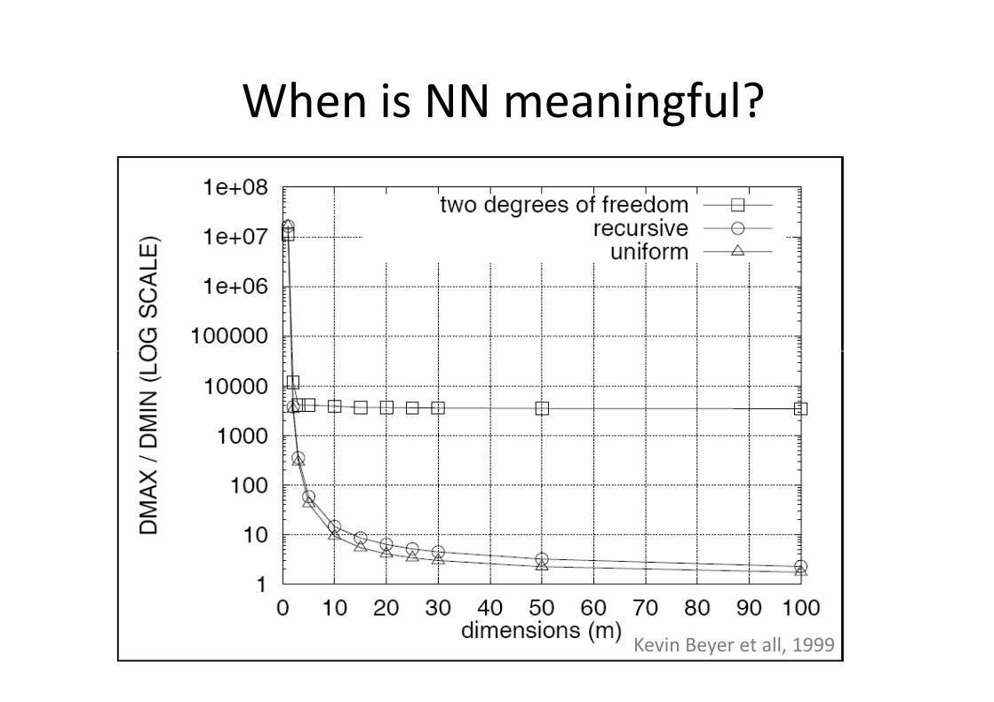
When is NN meaningful?
Kevin Beyer et all, 1999

What is the spell for the curse?
• Various attempts of multidimensional indexing
where proved that don’t make sense for a big
category of data distributions [CHRISTIAN BOHM, 2001]
• There has been a lot of research on • There has been a lot of research on
Dimensionality Reduction techniques.
• They basically apply ideas of compression, to
data, in order to reduce the dimensionality.
• In the next we will focus mainly in Time Series.

Introduction
11.5Euro-HK$ exchange rate
9
9.5
10
10.5
11
11.5
9/1/2011 10/1/2011 11/1/2011 12/1/2011 1/1/2012 2/1/2012
Euro-HK$ exchange rate
128-D
space
128 Data points
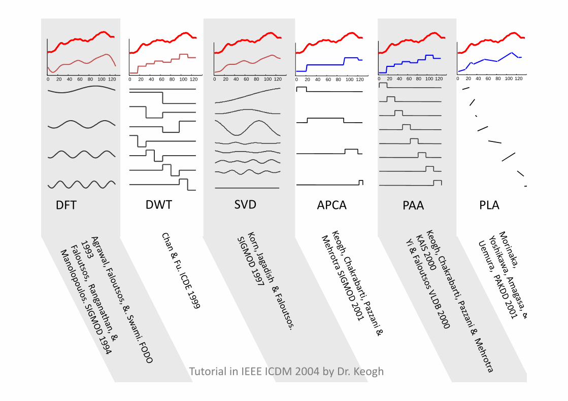
0 20 40 60 80 100 120 0 20 40 60 80 100 120 0 20 40 60 80 100 120 0 20 40 60 80 100 1200 20 40 60 80 100 120 0 20 40 60 80 100 120
DFT DWT SVD APCA PAA PLADFT DWT SVD APCA PAA PLA
Tutorial in IEEE ICDM 2004 by Dr. Keogh
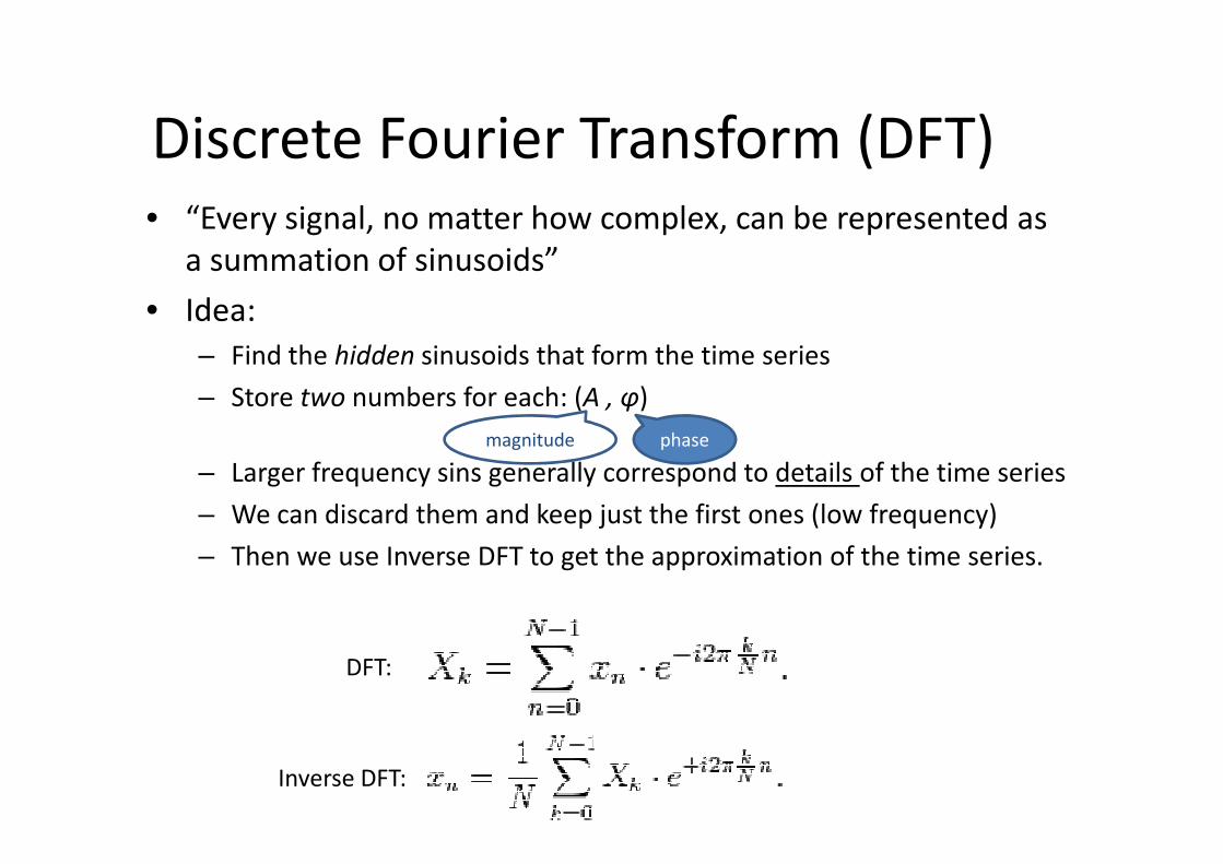
Discrete Fourier Transform (DFT)• “Every signal, no matter how complex, can be represented as
a summation of sinusoids”
• Idea:
– Find the hidden sinusoids that form the time series
– Store two numbers for each: (A , φ)
phasemagnitude
– Larger frequency sins generally correspond to details of the time series
– We can discard them and keep just the first ones (low frequency)
– Then we use Inverse DFT to get the approximation of the time series.
phasemagnitude
DFT:
Inverse DFT:

DFT example
9.5
10
10.5
11
11.5TIME SERIES
11.1934
11.2485
11.3186
11.2973
11.3036
11.3036
11.2025
11.1209
11.1012
11.0049
10.9885
A
1339.2
22.672
13.418
10.498
6.8649
3.5188
5.9621
5.5038
2.3058
3.238
1.3209
3.1939DFT
φ
0
-1.4846
-0.33742
-0.78383
-1.8342
-1.4738
-1.425
-1.2617
-1.7641
-1.8986
-1.0088
-1.588
9
9.5
1 7
13
19
25
31
37
43
49
55
61
67
73
79
85
91
97
10
3
10
9
11
5
12
1
12
7
10.9885
10.9401
10.9476
10.7698
10.6544
10.6476
10.7136
10.7492
10.72
10.6328
10.6849
10.6249
10.4904
10.4759
3.1939
2.818
0.34752
2.6411
3.1825
2.2584
2.0786
1.0066
1.25
1.4527
0.38684
1.8025
0.97202
1.3433
1.6972
DFT -1.588
-1.8385
-2.5873
-0.96067
-1.4374
-1.3702
-2.0808
-0.69754
-0.30255
-1.0405
0.092403
-1.2293
-0.31504
-0.24047
-1.6034
We store
8+8=16
values!

DFT example(cont)
IDFT
A
1339.2
22.672
13.418
φ
0
-1.4846
-0.33742
Approximate TS
10.824
10.949
11.059
11.147
11.21
11.243
11.248
11.226
11.181
11.118 9.5
10
10.5
11
11.5
DFT approximation
IDFT13.418
10.498
6.8649
3.5188
5.9621
5.5038
-0.33742
-0.78383
-1.8342
-1.4738
-1.425
-1.2617
11.043
10.963
10.883
10.809
10.746
10.695
10.657
10.632
10.618
10.611
10.609
10.607
10.603
10.594
10.579
9
9.5
1 6
11
16
21
26
31
36
41
46
51
56
61
66
71
76
81
86
91
96
10
1
10
6
11
1
11
6
12
1
12
6

DFT

DFT (pros & cons)
• O(nlogn) complexity
• Hardware Implementations
• Good ability to compress most signals
• Many applications
• Not good approximation for bursty signals
• Not good approximation if the signal contains both flat and busy segments
• Cannot support other distance metrics
• Contains info only for the frequency distribution– The time domain?

Why DFT is not enough?
• It gives us information about the frequency
component of a time series, without telling
where this frequency lies in the time domain1
z(t)=sin(5*t) , sin(10*t)2
x(t)=sin(5*t)+sin(10*t)3500
Fourier Decomposition (Spectrum)
0 1000 2000 3000 4000 5000 6000 7000-1
-0.8
-0.6
-0.4
-0.2
0
0.2
0.4
0.6
0.8
0 1000 2000 3000 4000 5000 6000 7000-2
-1.5
-1
-0.5
0
0.5
1
1.5
0 10 20 30 40 50 60 70 80 90 1000
500
1000
1500
2000
2500
3000
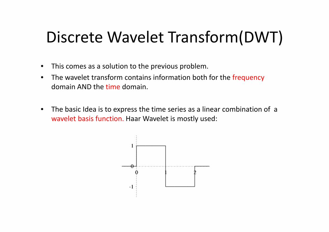
Discrete Wavelet Transform(DWT)
• This comes as a solution to the previous problem.
• The wavelet transform contains information both for the frequency
domain AND the time domain.
• The basic Idea is to express the time series as a linear combination of a
wavelet basis function. Haar Wavelet is mostly used:wavelet basis function. Haar Wavelet is mostly used:
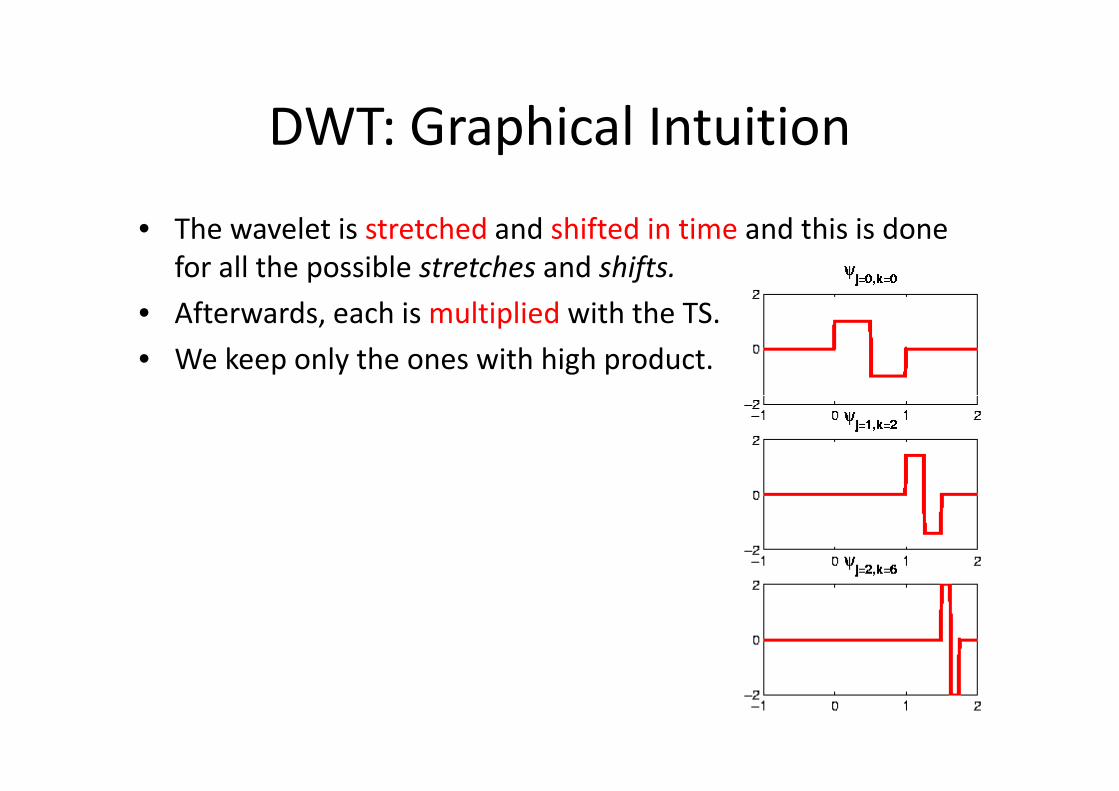
DWT: Graphical Intuition
• The wavelet is stretched and shifted in time and this is done
for all the possible stretches and shifts.
• Afterwards, each is multiplied with the TS.
• We keep only the ones with high product.
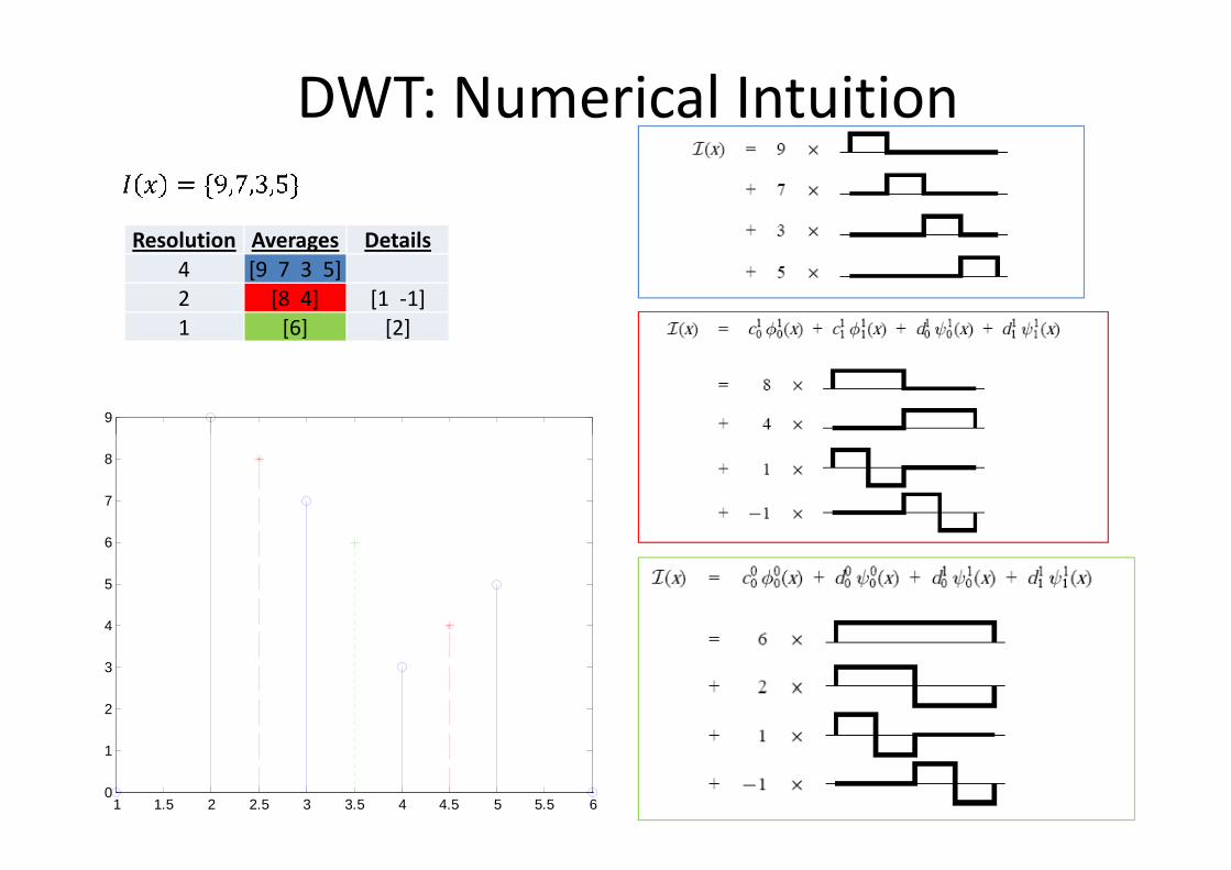
DWT: Numerical Intuition
Resolution Averages Details
4 [9 7 3 5]
2 [8 4] [1 -1]
1 [6] [2]
9
1 1.5 2 2.5 3 3.5 4 4.5 5 5.5 60
1
2
3
4
5
6
7
8

Example taken by Stollnitz, E. et all 1995
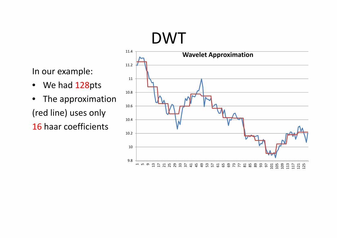
DWT
In our example:
• We had 128pts
• The approximation
(red line) uses only10.4
10.6
10.8
11
11.2
11.4Wavelet Approximation
16 haar coefficients
9.8
10
10.2
10.4
1 5 9
13
17
21
25
29
33
37
41
45
49
53
57
61
65
69
73
77
81
85
89
93
97
10
1
10
5
10
9
11
3
11
7
12
1
12
5
DWT(Pros & Cons)
• Good ability to compress stationary signals.• Fast linear time algorithms for DWT exist.
• Able to support some interesting non-Euclidean similarity measures.
• Signals must have a length n = 2some_integer
• Works best if N is = 2some_integer. Otherwise wavelets approximate the left side of signal at the expense of the right side.
• Cannot support weighted distance measures.

Singular Value Decomposition(SVD)
• All the previous methods, try to transform
each time series independently of the others.
• What if we take into account all the Time
Series contained in the Database?Series contained in the Database?
• We can then achieve the desired
dimensionality reduction for the specific
Dataset

SVD: Basic Idea [1]
q

SVD: Basic Idea (2)
q

SVD: Basic Idea (3)
q
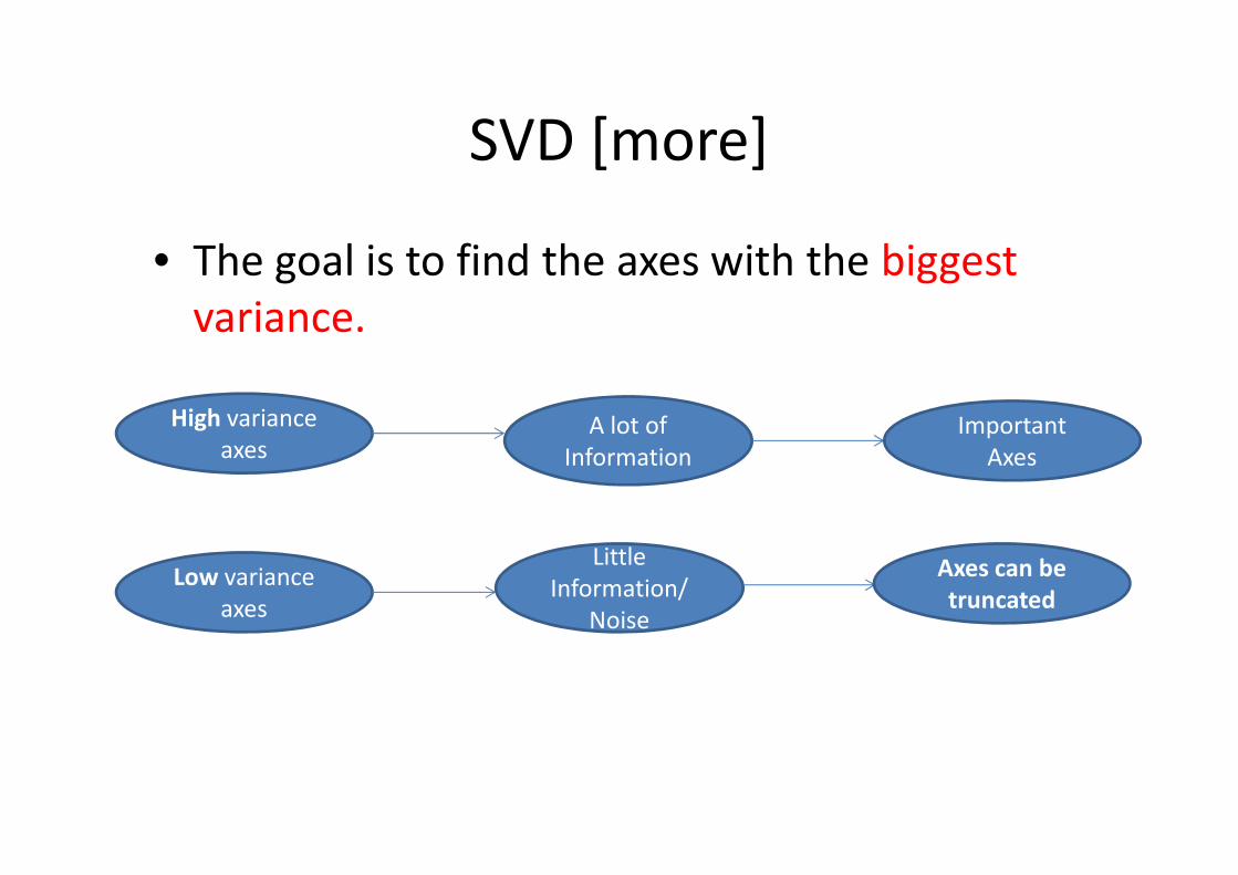
SVD [more]
• The goal is to find the axes with the biggest
variance.
High variance
axesA lot of Important
axesA lot of
Information
Low variance
axes
Little
Information/
Noise
Important
Axes
Axes can be
truncated
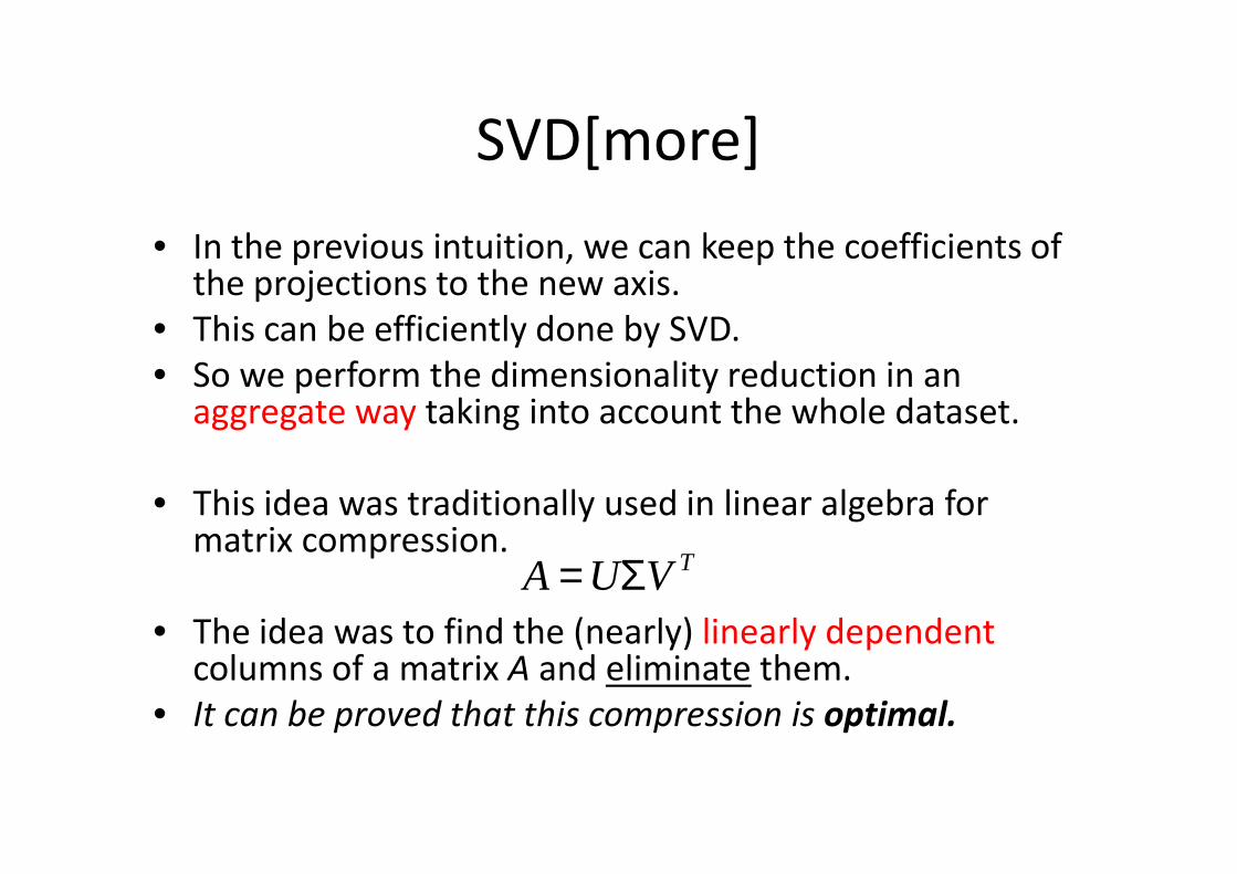
SVD[more]
• In the previous intuition, we can keep the coefficients of the projections to the new axis.
• This can be efficiently done by SVD.
• So we perform the dimensionality reduction in an aggregate way taking into account the whole dataset.
• This idea was traditionally used in linear algebra for matrix compression.
• The idea was to find the (nearly) linearly dependent columns of a matrix A and eliminate them.
• It can be proved that this compression is optimal.
TVUA Σ=
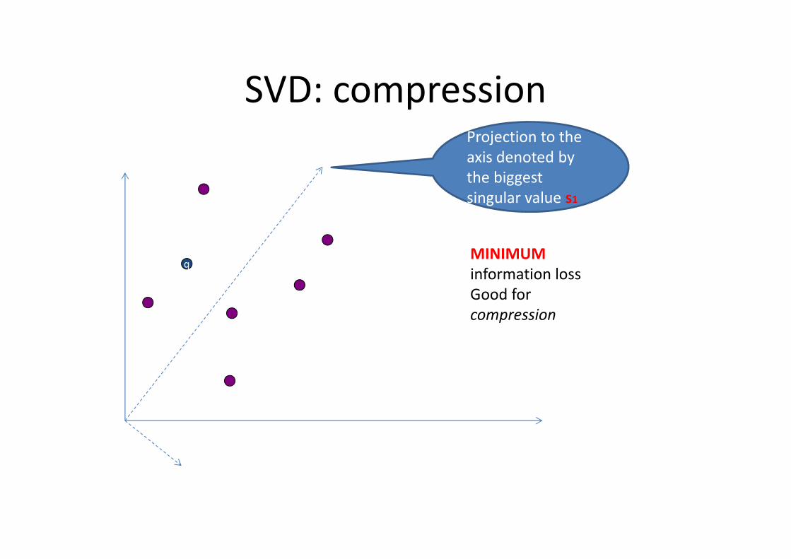
SVD: compression
q
Projection to the
axis denoted by
the biggest
singular value s1
MINIMUM
information lossinformation loss
Good for
compression

SVD: Clustering
q
Projection to the
axis denoted by
the smallest
singular value s2
MAXIMUM
information loss
Good for
clustering

SVD(Pros & Cons)
• Optimal linear dimensionality reduction technique .
• The eigenvalues tell us something about the underlying structure of the
data.
• Computationally very expensive.• Computationally very expensive.
• Time: O(Mn2)
• Space: O(Mn)
• An insertion into the database requires recomputing the SVD.
• Cannot support weighted distance measures or non Euclidean measures.
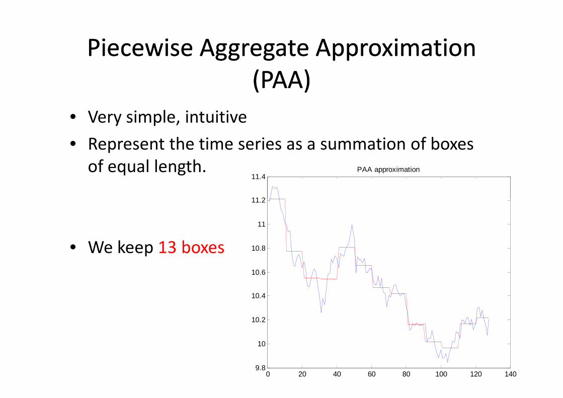
Piecewise Aggregate Piecewise Aggregate Approximation Approximation
(PAA)(PAA)
• Very simple, intuitive
• Represent the time series as a summation of boxes
of equal length.
11.2
11.4PAA approximation
• We keep 13 boxes
0 20 40 60 80 100 120 1409.8
10
10.2
10.4
10.6
10.8
11
11.2

PAA(Pros & Cons)
• Fast, easy to implement, intuitive
• The authors claim it is as efficient as other
approaches (empirically)
• Supports queries of arbitrary lengths• Supports queries of arbitrary lengths
• Supports non Euclidean measures
• It seems as a simplification of DWT, that
cannot be generalized to other types of signals
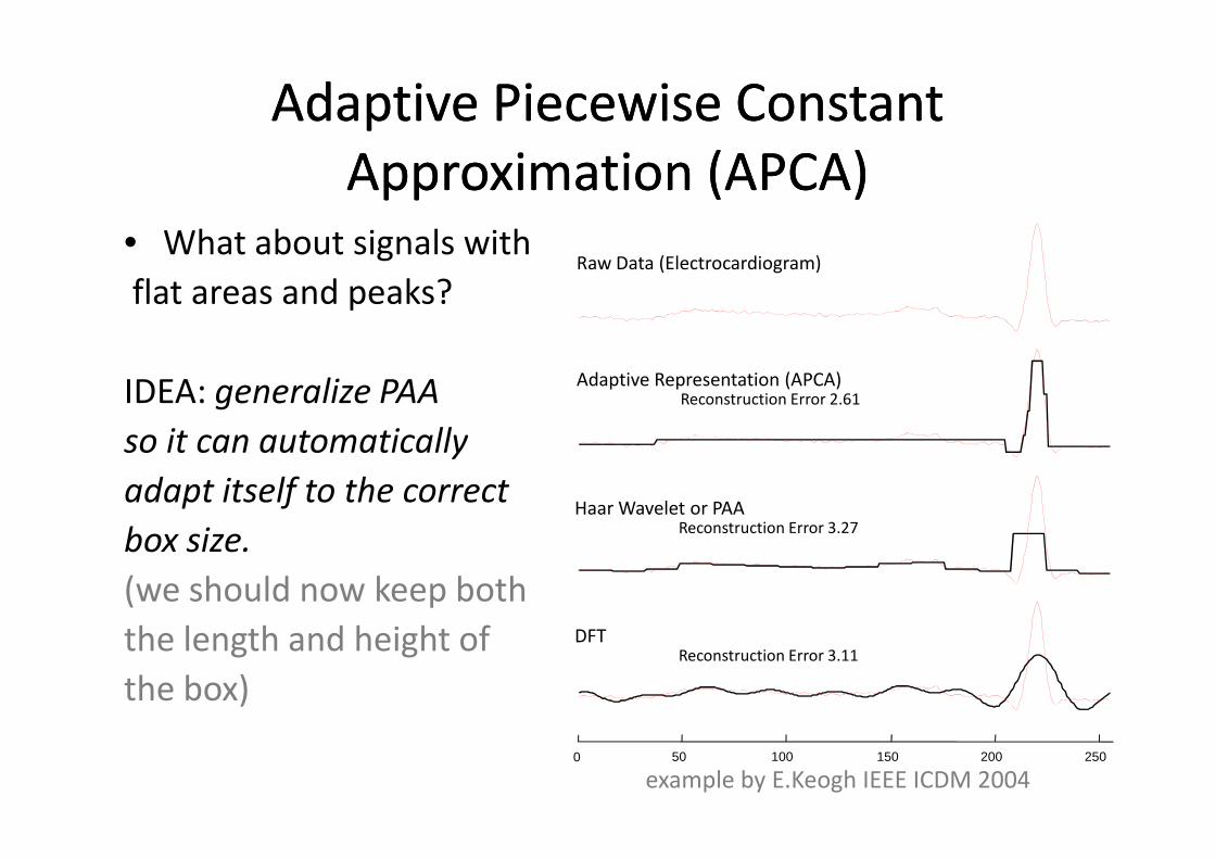
Adaptive Piecewise Constant Adaptive Piecewise Constant
Approximation (APCA)Approximation (APCA)• What about signals with
flat areas and peaks?
IDEA: generalize PAA
so it can automatically
Raw Data (Electrocardiogram)
Adaptive Representation (APCA)Reconstruction Error 2.61
so it can automatically
adapt itself to the correct
box size.
(we should now keep both
the length and height of
the box)
50 100 150 200 2500
Haar Wavelet or PAA Reconstruction Error 3.27
DFTReconstruction Error 3.11
example by E.Keogh IEEE ICDM 2004
APCA [more]
• In order to implement it, the authors propose
first a DWT transformation that is followed by
merging of the similar, adjacent wavelets.
• It is very efficient in some specific datasets• It is very efficient in some specific datasets
• However the indexing is more complicated
than PAA since we need two numbers for each
box.
• That is the reason why is not used very often.

Piecewise Linear Piecewise Linear Approximation (PLA)Approximation (PLA)
Linear segments
for representation
(not necessarily
connected)connected)
Although efficient in
some cases,
The implementation
is slow and it is not
indexableexample for visualization only

Non Linear Techniques
Dimensionality Reduction: A Comparative
Review, L.J.P. van der Maaten 2008
Non Linear techniques [2]
• A lot of techniques hve emerged the last
years.
• However , [Maaten et al 2008] compared
them with the PCA (equivalent to SVD) and in them with the PCA (equivalent to SVD) and in
most of the datasets all these complicated
techniques turn out to be worse.
• The reasons the authors claim, are data over
fitting and curse of dimensionality…

Conclusion
• All the before mentioned techniques have their strong and weak points.
• Dr Keogh tested them over 65 different datasets with different characteristics:
On average, they are all about the same. In particular, on 80% of the datasets they are all within 10% of each other.
So the choice for the best method depends on the characteristics of the Dataset