The Coyote Universe: Precision Simulations of the …cosmology.lbl.gov/talks/Heitmann_09.pdf · The Coyote Universe: Precision Simulations of the Large Scale Structure of the Universe

Katrin Heitmann, Los Alamos National Laboratory LBNL, March 12, 2009

The Coyote Universe:Precision Simulations of the Large Scale

Structure of the Universe

Katrin Heitmann, ISR-1, LANL

LBNL Seminar, March 12, 2009

In collaboration with:Suman Bhattacharya, Salman Habib, David Higdon,

Zarija Lukic, Earl Lawrence, Charlie Nakhleh, Christian Wagner, Martin White, Brian Williams

Visualization: Pat McCormick, CCS-1, LANL

SDSS, First Light in 1998 Deep Lens Survey/LSST

1998 2015


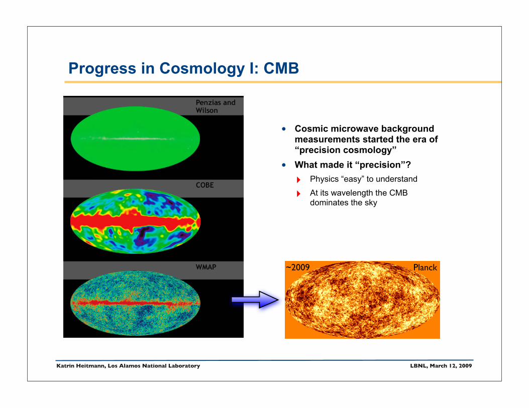
• Cosmic microwave background measurements started the era of “precision cosmology”

• What made it “precision”? ‣ Physics “easy” to understand

‣ At its wavelength the CMB dominates the sky

~2009 Planck

Progress in Cosmology I: CMB


• 1978: Discovery of voids and superclusters, theory of hierarchical structure formation via gravitational instability emerges

• 2006: SDSS has measured more than 1,000,000 galaxies, important discoveries such as the baryon oscillations by Eisenstein et al. cementing our picture of structure formation

Progress in Cosmology II: LSS

CfA, 1986 1,100 galaxies

De Lapparent, Geller, Huchra

Vo

id

Gregory & Thompson, 1978

SDSS

~1,000,000 galaxies

M. Blanton


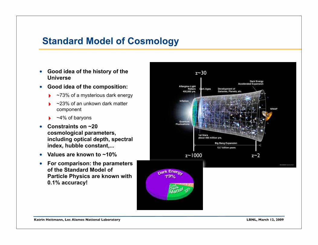
• Good idea of the history of the Universe

• Good idea of the composition:‣ ~73% of a mysterious dark energy

‣ ~23% of an unkown dark matter component

‣ ~4% of baryons

• Constraints on ~20 cosmological parameters, including optical depth, spectral index, hubble constant,...

• Values are known to ~10%

• For comparison: the parameters of the Standard Model of Particle Physics are known with 0.1% accuracy!

Standard Model of Cosmology

z~1000

z~30

z~2


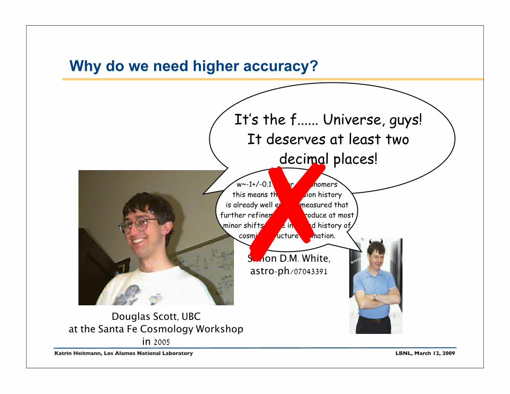
It’s the f...... Universe, guys!It deserves at least two

decimal places!

Douglas Scott, UBCat the Santa Fe Cosmology Workshop

in 2005

w~-1+/-0.1 .... for astronomers this means the expansion history

is already well enough measured that further refinement will produce at most minor shifts in the inferred history of

cosmics structure formation.

Simon D.M. White,

astro-ph/07043391

‘ ‘✗

Why do we need higher accuracy?


• Simple scaling arguments predict slope of the primoridal power spectrum to be n=1, constant, the Harrison-Zel’dovich power spectrum

• “Generic” inflationary models predict a slight deviation from n=1, usually smaller n < 1

• In addition: weak scale dependence, n(k), running• If we could measure the spectral index and its k-

dependence with high precision, we would have a smoking gun for inflation!

Why do we need higher accuracy?-- An example: The spectral index and inflation


• What is the nature of dark energy? ‣ Cosmological constant

‣ Scalar field

‣ Or none of this, but gravity is different on large scales..

• In the absence of a good idea: try to characterize dark energy

• We have to determine the dark energy equation of state, w and its time variation

• At the moment: w=-1+/-0.1 from different data sources, dw/dt consistent with zero

• Promising probes: baryon acoustic oscillations (power spectrum), clusters (mass function), supernovae, weak lensing (power spectrum)

Why do we need higher accuracy?-- Another example: Dark energy


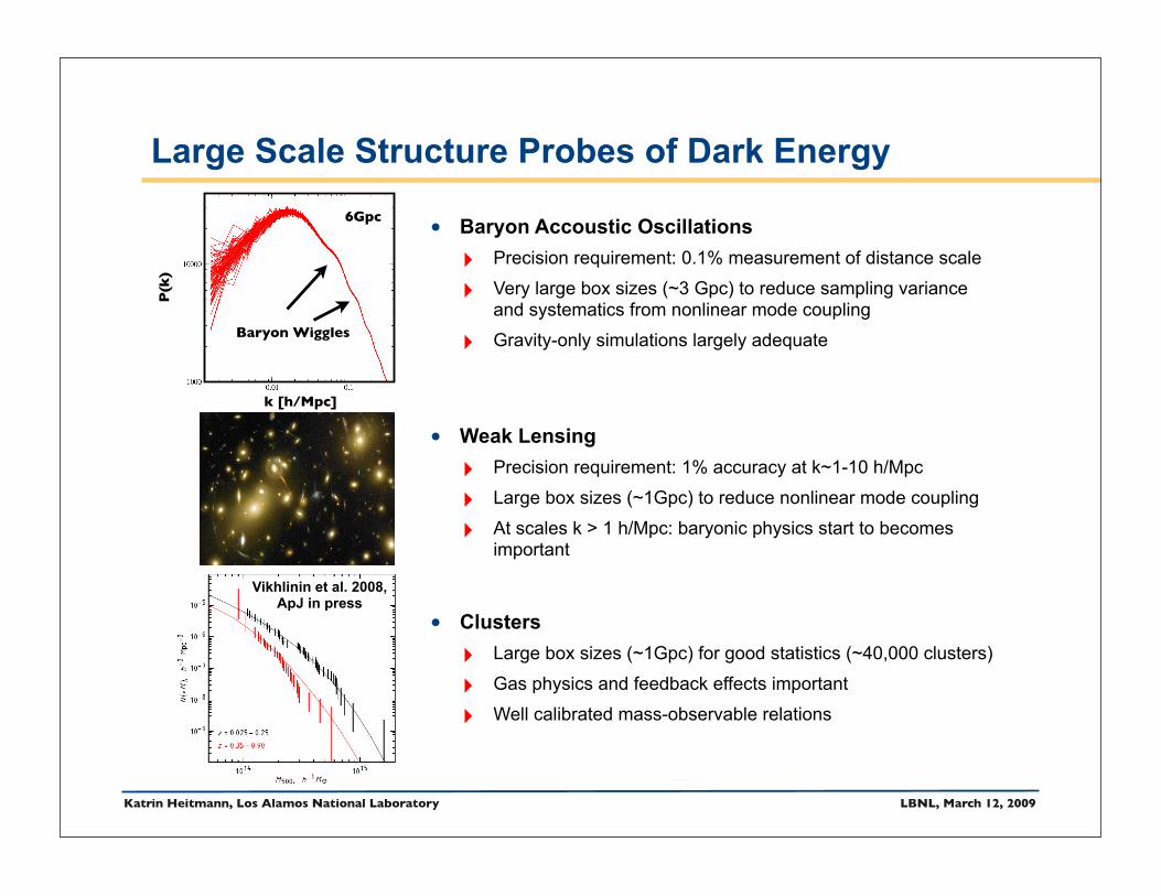
• Baryon Accoustic Oscillations‣ Precision requirement: 0.1% measurement of distance scale

‣ Very large box sizes (~3 Gpc) to reduce sampling variance and systematics from nonlinear mode coupling

‣ Gravity-only simulations largely adequate

• Weak Lensing‣ Precision requirement: 1% accuracy at k~1-10 h/Mpc

‣ Large box sizes (~1Gpc) to reduce nonlinear mode coupling

‣ At scales k > 1 h/Mpc: baryonic physics start to becomes important

• Clusters ‣ Large box sizes (~1Gpc) for good statistics (~40,000 clusters)

‣ Gas physics and feedback effects important

‣ Well calibrated mass-observable relations

Large Scale Structure Probes of Dark Energy

Vikhlinin et al. 2008, ApJ in press

Baryon Wiggles

k [h/Mpc]

P(k

)

6Gpc


SPT

BOSS

ACT

JDEM

Euclid

• JDEM‣ 2000 supernovae, 300-1000 square

degree lensing survey, w: ~4%, dw/dt:~10%

• SPT (Southpole Telescope)‣ 10 meter diameter telescope,

thousand clusters, strong constraints on w

• LSST (Large Synoptic Survey Telescope)‣ 8.4 meter, digital imaging across the

sky, supernovae, etc.

• DES (Dark Energy Survey)‣ Galaxy cluster study, weak lensing,

2000 SNe Ia, constraints on w at the one percent level

• Planck‣ High precision measurements of the

microwave background out to l~2500

Precision Cosmology: Observations


observerdoubtfultheorist

(from S. Furlanetto)

Huterer & Takada (2005) on requirements for future weak lensing surveys: “ While the power spectrum on

relevant scales (0.1 < k [h/Mpc] < 10) is currently calibrated with N-body simulations to about 5-10%, in

the future it will have to be calibrated to about 1-2%

accuracy ..... These goals require a suite of high resolution N-body simulations on a relatively fine grid in cosmological parameter space, and should be achievable in the near future.”

J. Annis et al: Dark Energy Studies: Challenges to Computational Cosmology (2005): Dark energy studies will challenge the computational cosmology community to critically assess current techniques, develop new approaches to maximize accuracy, and establish new tools and practices to efficiently employ globally networked computing resources.......Code comparison projects should be more aggressively pursued and the

sensitivity of key non-linear statistics to code control parameters deserves more careful systematic study......... Highly accurate dark matter evolution is only a first step

What about theory?


• “Billion/Billion” simulation:‣ Gigaparsec box, billion particles

‣ Smallest halos: ~10¹³ M (100 particles)

‣ 10 time snapshots: ~250GB of data

‣ ~30,000 Cpu hours with e.g. Gadget-2, ~5 days on 256 processors (no waiting time in the queue included...)

‣ Accuracy at k~1h/Mpc: ~1%

• 3 Gigaparsec, 300 billion particles‣ Smallest halos: ~10¹² M

‣ 10 time snapshots: ~75TB

• Physics:‣ Gravitational physics

‣ Gas physics

‣ Subgrid models

Great Survey Size Simulations

.

.


The Coyote Universe: Precision Predictions at the 1% level

• Large simulation suite run on LANL supercomputer “Coyote”‣ 38 cosmological models with different dark energy equations of state

‣ 1.3 Gpc cubed comoving volume, 1 billion particles each

‣ 16 medium resolution, 4 higher resolution, and 1 very high resolution simulation for each model = 798 simulations, ~60Tb of data

• Aim: precision predictions at the 1% accuracy level for different cosmological statistics‣ dark matter power spectrum out to k~1h/Mpc; on smaller scales: hydrodynamics effects

become important! (White 2004, Zhang & Knox 2004, Jing et al. 2006, Rudd et al. 2008)

‣ shear power spectrum

‣ mass function

• Three parts to the project:

‣ Demonstrate 1% accuracy of the dark mattter simulations out to k=1h/Mpc ✓ (arXiv:0812.1052)

‣ Develop framework which can predict these statistics from a minimal number of simulations ✓ (arXiv:09.02.0429)

‣ Build prediction tools from simulation suite (Coyote III, IV, in progress)

Coyote-I: arXiv:0812.1052, Coyote-II: arXiv:0902.0429 (submitted to ApJ), Coyote-III, IV: in preparation


Code ComparisonHeitmann et al., ApJS (2005); Heitmann et al., Comp. Science and Discovery (2008)

• Comparison of ten major codes (subset is shown)

• Each code starts from same initial conditions

• Each simulation is analysed in exactly the same way

• Overall, good agreement between codes for different statistics at the 5-10% level

0.1

1

10

100

1000

10000

P(k)[(Mpc/h)3]

HOTPKDGRAVHydra

Gadget-2

TPMTreePM

0.1 1 10k[h/Mpc]

-0.05

0

0.05

Residuals

64 Mpc/h256³ particles

2%

ParticleNyquist

Flash

PKDGRAV


Initial RedshiftHaroz, Ma & Heitmann (2008); Haroz & Heitmann (2008)

Early Start (z=250) Late Start (z=50)

z=10, Particles, Color: velocity

Line: Connect particle positions from the two outputs


Mass Resolution

• Test with different particle loading in 1Gpc box‣ Run 1024³ particles as reference

‣ Downsample to 512³ and 256³ particles and run forward

‣ In addition: downsample z=0,1 1024³ results to characterize shot noise problem

• For precision answers: interparticle spacing has to be small!

• Requirement: k < k_Ny/2

• Gigaparsec box requires billion particle minimum

• Force resolution is not the limiting factor, but mass resolution is

256³ particles k_Ny/2

512³ particles

z=1

z=0

Downsampled to 512³

Downsampled to 256³


• We have simulation accuracy under control at the 1% level out to k~1h/Mpc

‣ Mass resolution, box size, initial start, force resolution, and time step criteria exist!

• For cosmological constrains from e.g. SDSS:

‣ Run your favorite Markov Chain Monte Carlo code, eg. CosmoMC

- MCMC: directed random-walk in parameter space

‣ Need to calculate P(k) ~ 10,000 - 100,000 times for different models

‣ 30 years of Coyote time (2048 processor Beowulf Cluster), impossible!

• What we need: framework that allows us to provide, e.g., P(k) for a range of cosmological parameters

• The Cosmic Calibration Framework provides:

‣ Simulation design, an optimal strategy to choose parameter settings

‣ Emulation, smart interpolation scheme that will replace the simulator and will generate power spectra, mass functions... with controlled errors

‣ Uncertainty and sensitivity analysis

‣ Calibration -- combining simulations with observations to determine best-fit cosmology

The Cosmic Calibration FrameworkHeitmann et al., ApJL (2006); Habib et al., PRD (2007); Schneider et al., PRD (2008),

Heitmann et al., arXiv:0902.0429


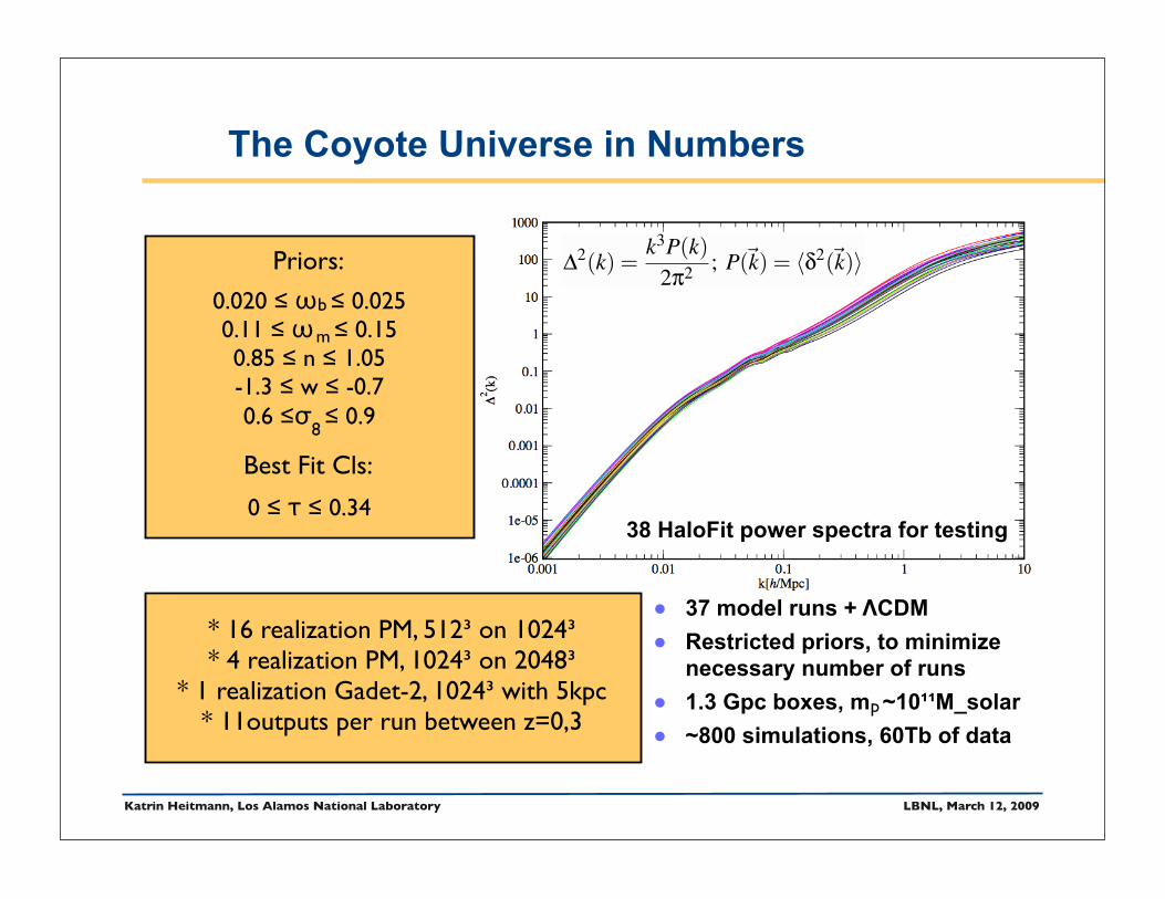
• 37 model runs + ΛCDM

• Restricted priors, to minimize necessary number of runs

• 1.3 Gpc boxes, m ~10¹¹M_solar

• ~800 simulations, 60Tb of data

0.020 ≤ ω ≤ 0.0250.11 ≤ ω ≤ 0.15 0.85 ≤ n ≤ 1.05-1.3 ≤ w ≤ -0.70.6 ≤σ ≤ 0.9

b

m

Priors:

8

Best Fit Cls:

0 ≤ τ ≤ 0.34

* 16 realization PM, 512³ on 1024³ * 4 realization PM, 1024³ on 2048³

* 1 realization Gadet-2, 1024³ with 5kpc* 11outputs per run between z=0,3

38 HaloFit power spectra for testing

p

The Coyote Universe in Numbers

!2(k) =k3P(k)

2"2 ; P(!k) = !#2(!k)"


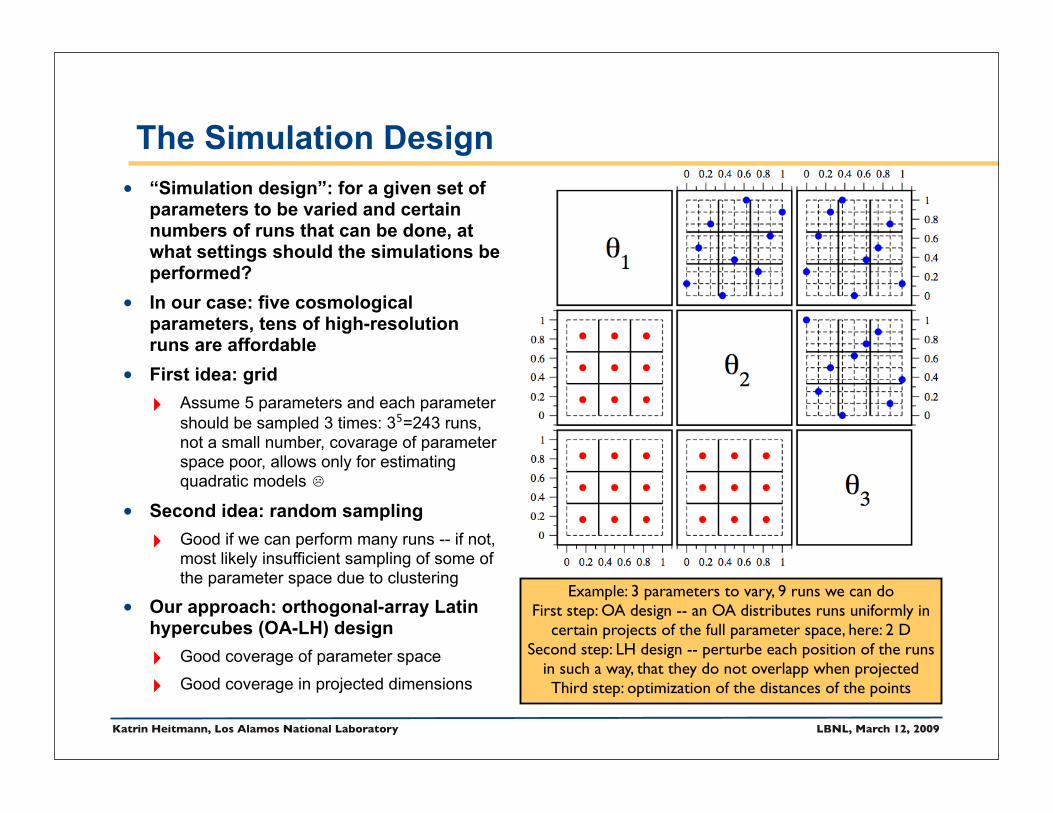
The Simulation Design• “Simulation design”: for a given set of

parameters to be varied and certain numbers of runs that can be done, at what settings should the simulations be performed?

• In our case: five cosmological parameters, tens of high-resolution runs are affordable

• First idea: grid ‣ Assume 5 parameters and each parameter

should be sampled 3 times: 3⁵=243 runs, not a small number, covarage of parameter space poor, allows only for estimating quadratic models ☹

• Second idea: random sampling‣ Good if we can perform many runs -- if not,

most likely insufficient sampling of some of the parameter space due to clustering

• Our approach: orthogonal-array Latin hypercubes (OA-LH) design‣ Good coverage of parameter space

‣ Good coverage in projected dimensions

Example: 3 parameters to vary, 9 runs we can doFirst step: OA design -- an OA distributes runs uniformly in

certain projects of the full parameter space, here: 2 DSecond step: LH design -- perturbe each position of the runs

in such a way, that they do not overlapp when projectedThird step: optimization of the distances of the points


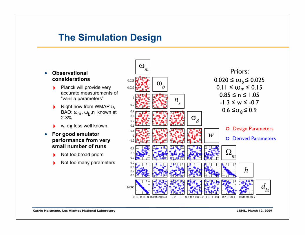
The Simulation Design

• Observational considerations‣ Planck will provide very

accurate measurements of “vanilla parameters”

‣ Right now from WMAP-5, BAO: ω , ω ,n known at 2-3%

‣ w, σ less well known

• For good emulator performance from very small number of runs‣ Not too broad priors

‣ Not too many parameters

0.020 ≤ ω ≤ 0.0250.11 ≤ ω ≤ 0.15 0.85 ≤ n ≤ 1.05-1.3 ≤ w ≤ -0.70.6 ≤σ ≤ 0.9

bm

Priors:

8

Design Parameters

Derived Parameters

bm

8


!!!"

!#$ #

%&

$!'!(!"$

)

*+,-

./012

.-13

!!!"

!#$ #

%&

$!$%"!$%#$

$%#

)

3415,6761#

./012

!1.-13

!!!"

!#$ #

%&

$!$%"!$%#$

$%#

)

3415,6761"

./012

!1.-13

!!!"

!#$ #

%&

$!$%"!$%#$

$%#

)

3415,6761!

./012

!1.-13

!!!"

!#$ #

%&

$!$%"!$%#$

$%#

)

3415,6761(

./012

!1.-13

!!!"

!#$ #

%&

$!$%"!$%#$

$%#

)

3415,6761&

./012

!1.-13

The Interpolation Scheme

• After having specified the simulation design: build interpolation scheme that allows for predictions for any cosmology within the priors

• Model simulation outputs using a - dimensional basis representation ‣ Find suitable set of orthogonal

basis vectors , here: principal componet analysis

‣ 5 PC bases needed, fifth PC basis pretty flat

‣ next step: modeling the weights

‣ Here: Gaussian Process modeling

p!

! [0,1]p!∈ln!

!2(k,z)2"k3/2

"=

p#

$i=1

%i(k,z)wi(&)+ '

Number of basis function, here: 5

Basis functions, here: PC basis

Weights, here: GP model

Cosmologicalparameters

Numberparameters, 5

!i(k,z)


Gaussian Process Models

w! N(0,!"1w R)

Ri j = exp{!||!i!! j||2}

Unconditioned GP: Conditioned GP:!

!!!

"" N

!0,

!K KT

!K!K!!

""

!!|!" N(K!K#1!,K!!K#1KT! )

• Nonparametric regression scheme, particularly well suited for interpolation of smooth functions

• Local interpolator, works well with space-filling sampling techniques

• Extending the notion of a Gaussian distribution over scalar or vector random variables into function space

• Gaussian distribution is specified by a scalar mean µ and a covariance matrix, GP specified by a mean function and a covariance function

*


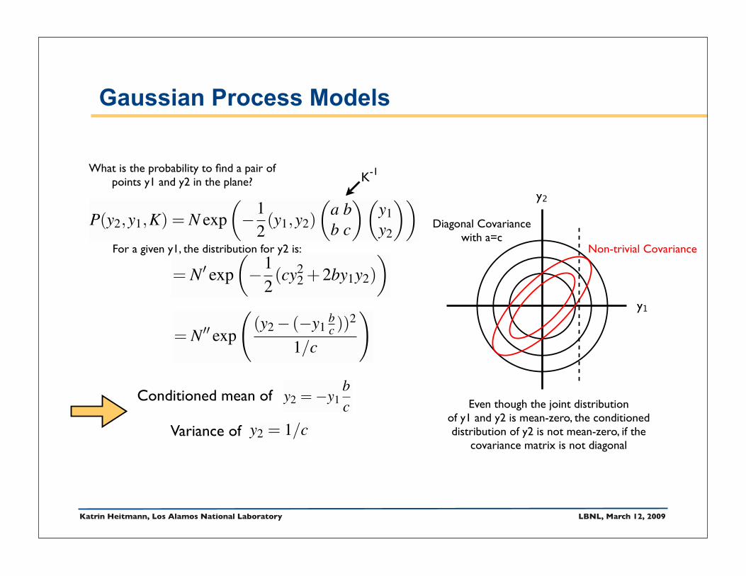
Gaussian Process Models

y₁

y₂

Diagonal Covariancewith a=c

Non-trivial Covariance

P(y2,y1,K) = N exp!!1

2(y1,y2)

!a bb c

"!y1y2

""K-1

= N! exp!"1

2(cy2

2 +2by1y2)"

= N!! exp

!(y2 " ("y1

bc ))2

1/c

"

Conditioned mean of

Variance of y2 = 1/c

y2 =!y1bc Even though the joint distribution

of y1 and y2 is mean-zero, the conditioned distribution of y2 is not mean-zero, if the

covariance matrix is not diagonal

What is the probability to find a pair of points y1 and y2 in the plane?

For a given y1, the distribution for y2 is:


Emulator Performance

1%

1%

• Emulator: interpolation scheme, which allows us to predict the power spectrum at non-simulated settings in the parameter space under consideration

• Build emulator from 37 HaloFit runs according to our design

• Generate 10 additional power spectra within the priors with Halofit and the emulator

• Emulator predictions are accurate at the sub-percent level!


• Three different resolutions: 16 realizations low resolution PM, 4 realization medium resolution PM, one high-resolution Gadget run

• Make sure that features are not washed out

• Construct smooth power spectra using a process convolution model (Higdon 2002)

• Basic idea: calculate moving average using a kernel whose width is allowed to change over to account for nonstationarity

• For very low k: sparse sampling and large scatter, difficult to handle

• Maybe: perturbation theory

The Smoothing Procedure

GadgetPM, 2048³PM, 1024³

Baryon wiggles

!2(k) =k3P(k)

2"2 ; P(!k) = !#2(!k)"


• To reduce run-to-run scatter: 30 realization of 2.78Gpc boxes with PM code

• Compare different perturbation theory ideas

• PT works well below 1% accuracy out to at least k=0.03/Mpc

Sim

ulat

ion/

Mat

suba

raSi

mul

atio

n/PT

M000

-2.0 -1.5 -1.0 -0.5

0.8

0.9

1.0

1.1

1.2

0.9

1.0

1.1

1.2

log₁₀(k)

Perturbation Theory for low k

Perturbation Theory valid

e.g, Peebles (1980)

Matsubara (2007)

For an excellent review of differentmethods and first full second order calculation, see: J. Carlson et al. 2009


log₁₀(P

(k))

Δ²

/Δ²

M0010.

90.

951.

01.

051.

10-4

.0-3

.5-3

.0-2

.5-2

.0-1

.5

-2.0 -1.5 -1.0 -0.5log₁₀(k)

pred

lin

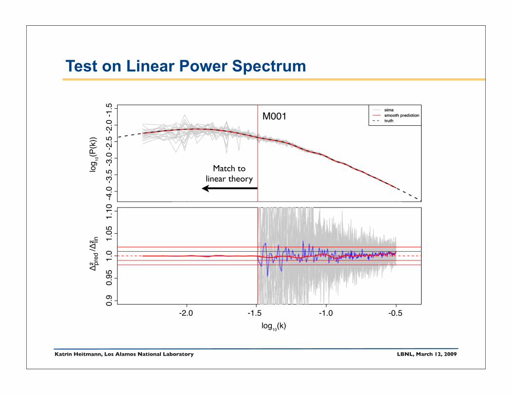
Test on Linear Power Spectrum

Match to linear theory


log₁₀(P

(k))

Δ²

/Δ²

M0320.

90.

951.

01.

051.

10-4

.0-3

.5-3

.0-2

.5-2

.0-1

.5

-2.0 -1.5 -1.0 -0.5log₁₀(k)

pred

lin

Test on Linear Power Spectrum


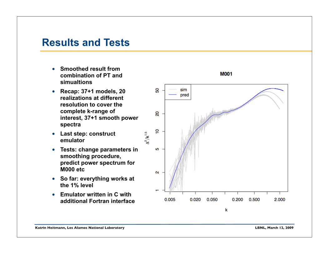
• Smoothed result from combination of PT and simualtions

• Recap: 37+1 models, 20 realizations at different resolution to cover the complete k-range of interest, 37+1 smooth power spectra

• Last step: construct emulator

• Tests: change parameters in smoothing procedure, predict power spectrum for M000 etc

• So far: everything works at the 1% level

• Emulator written in C with additional Fortran interface

Results and Tests


• Statistics describing the halo mass distribution in the Universe

• n(M): number density of halos with mass > M in a comoving volume element

• Evolution of mass function is highly sensitive to cosmology because matter density controls rate at which structure grows

• After Press/Schechter: semi-analytic fits by Sheth & Tormen (1999), Jenkins et al . (2001), Warren et al. (2006), Tinker et al. (2008) and many more...

• Dependence on halo definition, here overdensity (SO₁₈₀ )

Tinker et al. 2008Jenkins et al. 2001

The Halo Mass Function

ΛCDM Cosmology,Gadget run

b

z=1z=0.25

z=0

Preliminary!


Friends-of-friends, b=0.2Overdensity, M₂₀₀






The Halo Mass Function

Cosmology and z-dependence

z=1z=0.25z=0

Idea: build an emulator for mass function at different redshifts, different cosmologies, and different halo defintions (linking

length, overdensity)

10%

Comparison to Tinker et al. 2008, which was derived for w=-1,

agreement at z=0 at ~10%, slightly worse at higher z

z=0

Preliminary!

Preliminary!


The Next Step: The Roadrunner Universe


The Roadrunner Universe

The Roadrunner Universe is one of eight science projects

selected for first six months of runtime! Equivalent to 100

Million Cpu hours on conventional hardware


The Roadrunner Universe

• New hybrid P³M code

• Large suite of very large volume/large number of particle simulations with different cosmologies and realizations

• Lessons learnt from the Coyote Universe

• Large fraction of analysis needs to be done on the fly

• What information should be stored?

Collaboration: S. Habib, J. Ahrens, L. Ankeny, C.-H. Hsu, D. Daniel, N. Desai, P. Fasel, K.H., Z. Lukic, G. Mark, A. Pope


• Nonlinear regime of structure formation requires simulations‣ No error controlled theory

‣ Simulated skies/mock catalogs essential for survey analysis

• Simulation requirements are demanding, but can be met‣ Only a finite number of simulations can be performed

• Cosmic Calibration Framework ‣ Accurate emulation of several statistics matching code errors

‣ Allows fast calibration of models vs. data

• Future simulations‣ Very large data sets

‣ Emphasis on analysis, what should be done

‣ How should data be made available to the community?

Conclusions

Documents

The Coyote Universe: Precision Simulations of the …cosmology.lbl.gov/talks/Heitmann_09.pdf · The Coyote Universe: Precision Simulations of the Large Scale Structure of the Universe