Embed Size (px)
Citation preview

The Cost of Latency in High-Frequency Trading∗
Ciamac C. MoallemiGraduate School of Business
Columbia Universityemail: [email protected]
Mehmet SaglamBendheim Center for Finance
Princeton Universityemail: [email protected]
Current Revision: February 5, 2013
Abstract
Modern electronic markets have been characterized by a relentless drive towards faster de-cision making. Significant technological investments have led to dramatic improvements inlatency, the delay between a trading decision and the resulting trade execution. We describea theoretical model for the quantitative valuation of latency. Our model measures the tradingfrictions created by the presence of latency, by considering the optimal execution problem of arepresentative investor. Via a dynamic programming analysis, our model provides a closed-formexpression for the cost of latency in terms of well-known parameters of the underlying asset. Weimplement our model by estimating the latency cost incurred by trading on a human time scale.Examining NYSE common stocks from 1995 to 2005 shows that median latency cost acrossour sample roughly tripled during this time period. Furthermore, using the same data set, wecompute a measure of implied latency, and conclude that the median implied latency decreasedby approximately two orders of magnitude. Empirically calibrated, our model suggests thatthe reduction in cost achieved by going from trading on a human time scale to a low latencytime scale is comparable with other execution costs faced by the most cost efficient institutionalinvestors, and is consistent with the rents that are extracted by ultra low latency agents, suchas providers of automated execution services or high frequency traders.
1. Introduction
In the past decade, electronic markets have become pervasive. Technological advances in thesemarkets have led to dramatic improvements in latency, or, the delay between a trading decisionand the resulting trade execution. In the past 30 years, the time scale over which a trade isprocessed has gone from minutes1 to milliseconds2 — “low latency” in a contemporary electronicmarket would be qualified as under 10 milliseconds, “ultra low latency” as under 1 millisecond. Thischange represents a dramatic reduction by five orders of magnitude. To put this in perspective,human reaction time is thought to be in the hundreds of milliseconds.
One factor behind this trend has been competition between exchanges, as one mechanism fordifferentiation between exchanges is latency. This competition is driven by a significant demand∗The first author would like to thank Jim Gatheral for a helpful discussion that motivated this work. The authors
would like to thank Albert Menkveld, Larry Glosten, and Jialin Yu for their helpful comments.1NYSE, pre-1980 upgrade (Easley et al., 2008).2“The value of a millisecond: Finding the optimal speed of a trading infrastructure,” TABB Group, April 2008.
1
amongst a class of investors, sometimes called “high frequency” traders, for low latency tradeexecution. High frequency traders are thought to account for more than half of all US equitytrades.3 They expend significant resources in order to develop algorithms and systems that areable to trade quickly. For example, on the time scale of milliseconds, the speed of light can becomea binding constraint on the delay in communications. Hence, traders seeking low latency will “co-locate”, or house their computers in the same facility as the exchange, in order eliminate delaysdue to a lack of physical proximity. This co-location comes at a significant expense, however it hasbeen stated that a 1 millisecond advantage can be worth $100 million to a major brokerage firm.4
There has been much discussion of the importance of latency among various market participants,regulators, and academics. Despite the significant amount of recent interest, however, latencyremains poorly understood from a theoretical perspective. For example, how does latency relateto transaction costs? Is latency only relevant to investors with short time horizons, such as highfrequency traders, or does latency also affect long term investors such as pension funds and mutualfunds? Many of these important questions have been considered in anecdotal or ad hoc discussions.Our goal here is to provide a framework for quantitative analysis of these issues.
In particular, we wish to understand the benefit to a single trader in the marketplace of loweringtheir latency, while holding everything else fixed. This is a different question than understandingthe social costs of latency, i.e., whether in equilibrium the collective marketplace is better or worseoff given lower latency. One might imagine, for example, that the benefit to a individual agents oflower latency may diminish in an equilibrium setting. Equilibrium or welfare analysis of low latencytrading is a complex question with important policy and regulatory implications. We believe thatunderstanding the single-agent effects of low latency trading, however, is an important first stepwhich will inform our ultimate understanding of collective effects.
The cost that a trader bears due to latency can take many different forms, depending onthe precise trading strategy. However, we can identify a number of broad themes,5 sometimesoverlapping, as to why the ability to trade with low latency might be valuable to an investor:
1. Contemporaneous decision making. A trader with significant latency will be makingtrading decisions based on information that is stale.
For example, consider an automated trader implementing a market-making strategy in anelectronic limit order book. The trader will maintain active limit orders to buy and sell. Theprices at which the trader is willing to buy or sell will naturally depend on, say, the limitorders submitted by other investors, the price of the asset on other exchanges, the price ofrelated assets, overall market factors, etc. If the trader cannot update his orders in a timelyfashion in response to new information, he may end up trading at disadvantageous prices.
2. Comparative advantage/disadvantage. The ability to trade with low latency in absolute3“Stock traders find speed pays, in milliseconds,” New York Times, July 23, 2009.4“Wall Street’s quest to process data at the speed of light,” Information Week, April 21, 2007.5See Cespa and Foucault (2008) for a related discussion.
2
terms may not be as important as the ability to trade with low relative latency, that is, ascompared to competitors.
For example, consider a program trader implementing an index arbitrage strategy, seekingto profit on the difference between an index and its underlying components. There may bemany market participants pursuing such strategies and identifying the same discrepancies.The challenge for the trader is to be able to act in the marketplace to exploit a discrepancybefore a price correction takes place, i.e., before competitors are able to act. The meanshaving a low relative latency.
3. Time priority rules. Many modern markets treat orders differentially based on the timeof arrival, and favor earlier orders.
For example, in an electronic limit order book, the limit orders on each side of the marketare prioritized in a particular way. When a market order to buy arrives, it is matched againstthe limit orders to sell according to their priorities. Priority is first determined by price,i.e., limit orders with more lower prices receive higher priority. In many markets, however,prices are mandated to be discrete with a minimum tick size. In these markets, there may bemultiple limit orders at the same price, which are then prioritized according to the time oftheir arrival. While a trader can always increase the priority of his orders by decreasing price,this comes at an obvious cost. If a trader can submit orders in a faster fashion, however, hecan increase priority while maintaining the same price. Higher priority can be valuable fortwo reasons: first, higher priority orders have a higher likelihood of execution over any giventime horizon. To the extent that investors submitting limit orders have a desire to trade, andto trade sooner rather than later, this is desirable. Second, higher priority orders at the sameprice level experience less adverse selection (see, e.g., Glosten, 1994; Sandås, 2001). Hence,all things being equal, an investor who submits orders with lower latency will benefit fromhigher priority than if that investor had higher latency. This can be particularly important(in that a small improvement in latency can result in a significant difference in priority) whenan existing quote is about to change. For example, consider the situation where a stock priceis about to move up because of trades or cancellations at the best offered price. One mightexpect the bid price to rise as well, there will be a race among traders reacting to the sameorder book events to establish time priority at the new bid.
In this paper, we will quantify the cost of latency due to the first effect, a lack of contemporane-ous decision making. We do not consider effects of latency that arise from strategic considerations,or from time priority rules or price discreteness. It is an open question as to whether the othereffects are more or less significant than the first, and their relative importance may depend on theparticular investor and their trading strategy. Our analysis does not speak to this point. However,in what follows we will demonstrate that, by itself, the lack of contemporaneous decision makingcan induce trading costs that are of the same order of magnitude as other execution costs faced by
3

large investors, and hence cannot be neglected.Further, the importance of contemporaneous decision making will certainly vary from investor
to investor. We will focus on an aspect of this that is universal, however, which is the importanceof timely information for the execution of contingent orders. A contingent order, such as a limitorder in an electronic limit order book or a resting order in a dark pool, presents the possibility ofuncertain execution over an interval of time in exchange for price improvement relative to a marketorder, which executes immediately and with certainty. Specifically, when an investor employs acontingent order, the investor may be exposed to the realization of new information (for example,in the form of price movements, news, etc.) over the lifespan of the order. Latency, which preventsthe investor from continuously and instantaneously accessing the market so as to update the order,can thus adversely impact the investor.
As a broad proxy for understanding the importance of latency in contingent order execution,we consider the effects of latency in an extremely simple yet fundamental trade execution problem:that of a risk-neutral investor who wishes to sell 1 share of stock (i.e., an atomic unit) over a fixed,short time horizon (i.e., seconds) in a limit order book, and must decide between market ordersand limit orders. Our problem formulation is reminiscent of barrier-diffusion models for limit orderexecution (e.g., Harris, 1998). It captures the fundamental cost of immediacy of trading (e.g.,Grossman and Miller, 1988; Chacko et al., 2008), that is, the premium due to a patient liquiditysupplier (who submits limit orders) relative to an impatient demander of liquidity (who submitsmarket orders). While this problem is quite stylized, we will argue that it is broadly relevant since,at some level, all investors make such a choice of immediacy. For example, it may not seem at firstglance that our execution problem is relevant for a pension fund that trades large blocks of stockover multiple days. However, the execution of a block trade via algorithmic trading involves thedivision of a large “parent” order into many atomic orders over the course of a day, each of theseatomic “child” orders can be executed as limit orders or as market orders.
In our problem, in the absence of latency, the optimal strategy of the seller is a “pegging”strategy: the seller maintains a limit order at a constant spread above the bid price at any instantin time. We consider this case as a benchmark. In the presence of latency, the seller can no longermaintain continuous contact with the market so as to track the bid price in the market. Theseller is forced to deviate from the benchmark policy in order to take into account the uncertaintyintroduced by the latency delay by incorporating a safety margin and lowering his limit order prices.The friction introduced by latency thus results in a loss of value to the seller. We will establish thedifference in value to the seller between the case with latency and the benchmark case via dynamicprogramming arguments, and thus provide a quantification of the effects of latency.
The contributions of this paper are as follows:
• We mathematically quantify the cost of latency.
The trading problem we consider (deciding between limit and market orders) is faced by alllarge investors in modern equity markets, either directly (e.g., high frequency traders) or
4
indirectly (e.g., pension funds who execute large trades via providers of automated executionservices). Our analysis suggests that latency impacts all of these market participants, andthat, all else being equal, the ability to trade with low latency results in quantifiably lowertransaction costs. Further, when calibrated with market data, the latency cost we measurecan be significant. It is of the same order of magnitude as other trading costs (e.g., commis-sions, exchange fees, etc.) faced by the most cost efficient large investors. Moreover, it isconsistent with the rents that are extracted by agents who have made the requisite technolog-ical investments to trade with ultra low latency. For example, the latency cost of our modelis comparable to the execution commissions charged by providers that offer algorithmic tradeexecution services on an agency basis. It is also comparable to the reported profits of highfrequency traders.
To our knowledge, our model is the first to provide a quantification of the costs of latency intrade execution.
• We provide a closed-form expression for the cost of latency as a function of well-known pa-rameters of the asset price process.
The cost of latency in our model can be computed numerically via dynamic programming.However, in the regime of greatest interest, where the latency is close to zero, we provide aclosed-form asymptotic expression. In particular, define the latency cost associated with anasset as the costs incurred due to latency as a fraction of the overall cost of immediacy (thepremium paid to a patient liquidity supplier by an impatient demander of liquidity). Givena latency of ∆t, a price volatility of σ, and a bid-offer spread of δ, the latency cost takes theform
(1) σ√
∆tδ
√log δ2
2πσ2∆t
as ∆t→ 0.
• Our method can provide qualitative insight into the importance of latency.
From (1), it is clear that the latency cost is an increasing function of the ratio of the standarddeviation of prices over the latency interval (i.e., σ
√∆t) to the bid-offer spread. Latency
has a more important role when trading assets that are either more volatile (σ large) or,alternatively, more liquid (δ small). Further, as the latency approaches 0, the marginalbenefit of latency reduction is increasing.
• We empirically demonstrate that latency cost incurred by trading on a human time scale hasdramatically increased for U.S. equities and the implied latency of a representative trader inthis market decreased by approximately two orders of magnitude.
5
We consider the cost due to the latency of trading on the time scale of human interaction.Usingthe data-set of Aït-Sahalia and Yu (2009), we estimate the latency cost of NYSE commonstocks over the 1995–2005 period. We show that the median latency cost roughly tripled inthis time. This coincides with a period of decreasing tick sizes and increasing algorithmic andhigh frequency trading activity (Hendershott et al., 2010).
An alternative perspective is to consider a hypothetical investor who fixes a target level of costdue to latency, relative to the overall cost-of-immediacy. The representative trader maintainsthis target over time through continual technological upgrades to lower levels of latency. Wedetermine the requisite level of implied latency for such a trader, over time and across theaggregate market. Using the same data-set, we observe that the median implied latencydecreased by approximately two orders of magnitude over this time frame.
The rest of this paper is organized as follows: In Section 1.1, we review the related literature. InSection 2, as a starting point, we present a stylized, continuous-time trade execution problem in theabsence of latency. We develop a variation of the model with latency in Section 3. In Section 4, weprovide a mathematical analysis of the optimal policy for our problem. By contrasting the resultsin the presence and absence of latency, we are able to quantitatively assess the cost of latency. InSection 5, we consider some empirical applications of the model. Finally, in Section 6 we concludeand discuss some future directions.
1.1. Related Literature
There has been a significant empirical literature studying, broadly speaking, the effects of improve-ments in trading technology. Closest to the aspect we consider is the work of Easley et al. (2008).They empirically test the hypothesis that latency affects asset prices and liquidity by examining thetime period around an upgrade to the New York Stock Exchange technological infrastructure thatreduced latency. Hendershott et al. (2010) explore the more general, overall effects of algorithmicand high frequency trading. Hasbrouck and Saar (2009) provide different evidence of changes ininvestor trading strategies that may be a result of improved technology. In subsequent work, theyfurther consider the impact of measurements of low latency on market quality (Hasbrouck and Saar,2010). Hendershott and Riordan (2009) analyze the impact of algorithmic trading on the price for-mation process using a data set from Deutsche Börse and conclude that algorithmic trading assistsin the efficient price discovery without increasing the volatility. Kirilenko et al. (2010) consider theimpact of high frequency trading on the ‘flash crash’ of 2010, while Brogaard (2010) more broadlyexamines the impact of high frequency traders on market quality.
On the theoretical front, Cespa and Foucault (2008) consider a rational expectations equi-librium between investors with different access to past transaction data. Some investors observetransactions in real-time, while others only observe transactions with a delay. This model of latencyfocuses on latency of the price ticker of past transactions, as opposed to latency in execution, which
6
we consider here. Moreover, the goals of the two models differ significantly: Cespa and Foucault(2008) seek to build intuition regarding the equilibrium welfare implications of differential accessto information via a structural model. We, on the other hand, seek a reduced form model that canbe used to directly estimate the value of execution latency in a particular real world instance, givenreadily available data. Also related is the work of Ready (1999) and Stoll and Schenzler (2006), whoconsider the ability of intermediaries (e.g., specialists or dealers) to delay customer orders for theirown benefit, thus creating a “free option” in the presence of execution latency. Cohen and Szpruch(2011) show that latency arbitrage exists between two traders with different speeds of trading inthe presence of a limit order book. Finally, Cvitanic and Kirilenko (2010) and Jarrow and Protter(2011) consider the effect of high frequency traders on asset prices.
The trade execution problem we consider is that of an investor who wishes to sell a single shareof and must decide between market and limit orders. This problem has been considered by manyothers (e.g., Angel, 1994; Harris, 1998; Lo et al., 2002). Our formulation is similar to the class ofbarrier-diffusion models considered by these authors; Hasbrouck (2007) provides a good accountof this line of work. For a broad survey on limit order markets, see Parlour and Seppi (2008).In our model, the inability to trade continuously gives a limit order an option-like quality thatrelates execution cost, order duration, and asset volatility. This idea goes as far back as the workof Copeland and Galai (1983). Closely related is the concept of the cost of immediacy, or, thepremium paid by a liquidity demander via a market order to a liquidity supplier who posts a limitorder. Grossman and Miller (1988) and Chacko et al. (2008) develop theoretical explanations ofthe cost of immediacy. For empirical evidence of the demand for immediacy in capital markets, seeBacidore et al. (2003) and Werner (2003).
Finally, also related is work on the discrete-time hedging of contingent claims with or withouttransaction costs (e.g., Boyle and Emanuel, 1980; Leland, 1985; Bertsimas et al., 2000). Thisliterature addresses a different problem and draws different conclusions than our paper, howeverboth relate to implications of a lack of continuous access to the market.
2. A Stylized Execution Model without Latency
Our goal is to understand the impact on the trade execution of latency. To this end, we will firstdescribe a trade execution problem in the absence of latency. In Section 3, we will revisit this modelin the presence of latency, so as to understand the resulting trade friction that is introduced. Thespirit of our model it to consider an investor who wants to trade, but at a price that depends on aninformational process that evolves stochastically and must be monitored continuously. We coulddirectly consider such an abstract model of investor behavior. Instead, however, we will motivatethe informational dependence of the trader through a specific optimal execution problem.
Consider the following stylized execution problem of an uninformed trader who must sell exactly
7
one share6 of a stock over a time horizon [0, T ]. At any time t ∈ [0, T ), the trader can take one oftwo actions:
1. The trader can submit a market order to sell. This order will execute at the best bid priceat time t, denoted by St. We assume that the bid price evolves according to
(2) St = S0 + σBt,
where the process (Bt)t∈[0,T ] is a standard Brownian motion and σ > 0 is an (additive) volatil-ity parameter. Here, the choice of Brownian motion is made for simplicity; our model can beextended to the more general class of Markovian martingales, as discussed in Section 4.4.
2. The trader can choose to submit a limit order to sell. In this case, the trader must also decidethe limit price associated with the order, which we denoted by Lt.
Once the trader sells one share, he exits the market. If the trader is not able to sell 1 share beforetime T , however, we assume that he is forced sell via a market order at time T , and thereforereceives ST . Here, we imagine the time horizon T to be small, on the order of the typical tradeexecution time (i.e., seconds).
2.1. Limit Order Execution
It remains to describe the execution of limit orders. In our setting, a limit order can execute in oneof the following two ways:
1. We assume that there are impatient buyers who arrive to the market according to a Poissonprocess with rate µ. Denote by (Nt)t∈[0,T ) the cumulative arrival process for impatient buyers.Each impatient buyer seeks to buy a single share. An arriving impatient buyer arriving attime t has a reservation price St + zt, expressed as a premium zt ≥ 0 above the bid priceSt that the buyer is willing to forgo in order to achieve immediate execution. We assumethat the premium zt is independent and identically distributed with cumulative distributionfunction F : R+ → [0, 1]. In this setting, the instantaneous arrival rate of impatient buyersat time t willing to pay a limit order price of Lt is given by
(3) λ(ut) , µ(1− F (ut)
),
where ut , Lt − St is the instantaneous price premium of the limit order. In what follows,6Note that the trade quantity of a single share is meant to represent an atomic unit of the asset, or the smallest
commonly traded lot size. The underlying assumption is that the desired trade execution will ultimately be accom-plished by a single transaction. In typical U.S. equity markets, for example, this atomic unit might be a block of 100shares.
8

t0 T
St
Lt
Sτ1 + δ
τ1
Sτ2 + δ
τ2 τ3
market orders arrive
limit order executes
Figure 1: An illustration of the limit order execution in the stylized model over the time horizon [0, T ].Here, we assume the trader leaves a limit order with the (constant) price Lt and St is the bid priceprocess. If market orders arrive at times τ1 and τ2, the limit order would execute at time τ2 but nottime τ1, since the limit order price is in excess of δ to the best bid price. The limit order would alsoexecute at time τ3 in the absence of a market order arrival, since the bid price crosses the limit orderprice at this time.
we will be particularly interested in the special case where
(4) λ(ut) ,
µ if ut ≤ δ,
0 otherwise.
Here, we assume that every impatient buyer is willing to pay a price premium of at mostδ > 0. We assume that δ will be specific to the security and fixed for the trading horizon.We will discuss the extension to the general case (3) in Section 4.4.
Given (4), an impatient buyer is willing to buy 1 share at a fixed premium δ > 0 to the bidprice at the time of their arrival. Hence, if a buyer arrives at time τ ∈ [0, T ), and the traderhas placed a limit order with price Lτ , the limit order will execute if Lτ ≤ Sτ + δ.
2. Alternatively, a limit order will also execute at time τ if the bid price crosses the limit orderprice, i.e., Sτ ≥ Lτ .
The execution of limit orders in the model is illustrated in Figure 1.The limit order execution dynamics above can also be economically interpreted in the spirit
of the non-informational trade model of Roll (1984). In particular, imagine that the asset has afundamental value Vt at time t, and that Vt evolves exogenously according to the additive randomwalk
Vt = V0 + σBt.
If all investors observe this underlying value process and are symmetrically informed, competitivemarket makers will always be willing to sell shares at a price of δ/2 above the fundamental value
9

or buy shares at a spread of δ/2 below the fundamental value. Here, the quantity δ captures theper share operating costs of trade to the market markers. The liquidating trader can thus sell atthe bid price St = Vt − δ/2 at any time t. We assume that all other traders in the market areimpatient, and that these traders arrive according to the Poisson dynamics described above. Anarriving impatient buyer will choose to purchase from the liquidating trader only at a price lowerthan that provided by the market makers, i.e., only below the price of Vt+δ/2 = St+δ. In this way,we can interpret the parameter δ as the prevailing bid-offer spread, that is, the bid-offer spread inthe absence of the liquidating trader.
2.2. Optimal Solution
Let P denote the random variable associated with the sale price. We assume the trader is risk-neutral and seeks to maximize the expected sale price. Equivalently, we assume the trader seeksto solve the optimization problem
(5) h0 , maximize E [P ]− S0.
Here, the maximization is over policies of market orders and limit orders which are non-anticipating,i.e., policies adapted to the filtration generated by the underlying market primitives, (Bt, Nt)t∈[0,T ].This objective is equivalent to minimizing implementation shortfall (Perold, 1988).
Note that, while this stylized problem may seem quite simplified, it seeks to answer a funda-mental question: at the level of an atomic unit of stock and over a short time horizon, how shoulda risk-neutral investor choose between limit orders and market orders? This problem is a centralingredient in more sophisticated optimal execution problems involving risk averse investors sellinglarge quantities over longer time horizons.7 This is because, in a typical algorithmic trading setting,a large “parent” order will be scheduled across time into many very small “child” orders. Each ofthese “child” orders need to be executed optimally. Since each child order is small and since thereare many such child orders, it is reasonable to view the investor as risk-neutral with respect to eachchild order.
The following lemma characterizes a simple strategy that is optimal for the execution problemwe have described:
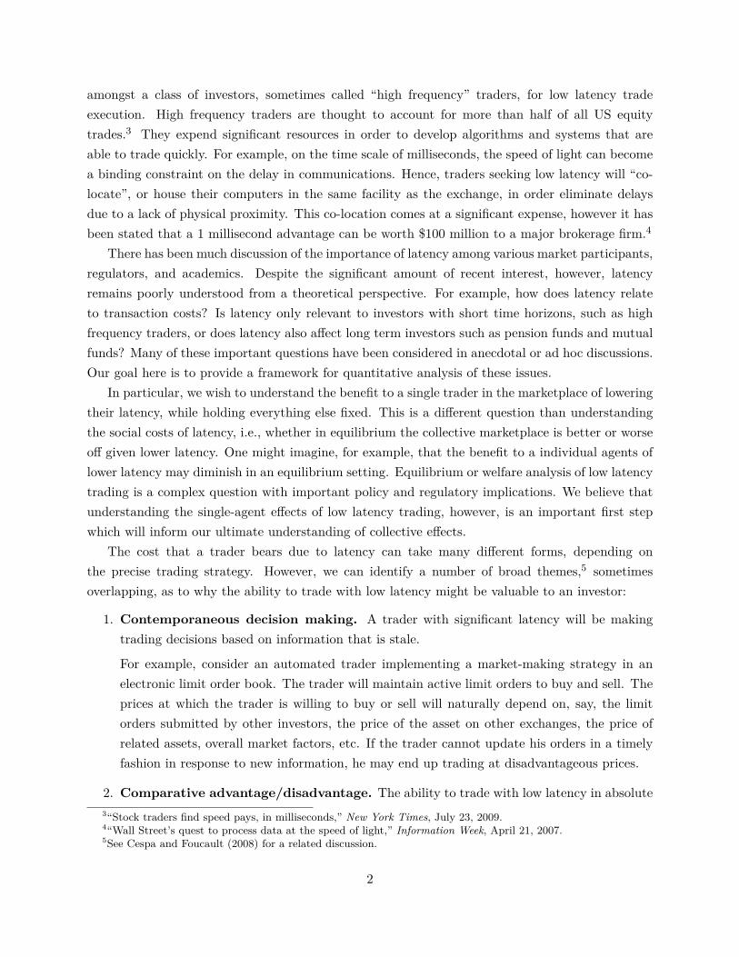
Lemma 1. An optimal strategy is to employ only limit orders at times t ∈ [0, T ), with limit priceLt = St + δ. In other words, the limit order price is “pegged” at a constant premium δ above thebid price. This pegging strategy achieves the optimal value
(6) h0 = δ(1− e−µT
).
7For example, see Bertsimas and Lo (1998) or Almgren and Chriss (2001). These questions have also recentlybeen addressed by Back and Baruch (2007) and Pagnotta (2010) in equilibrium settings.
10
t0 T
St
Lt
Lt = St + δ
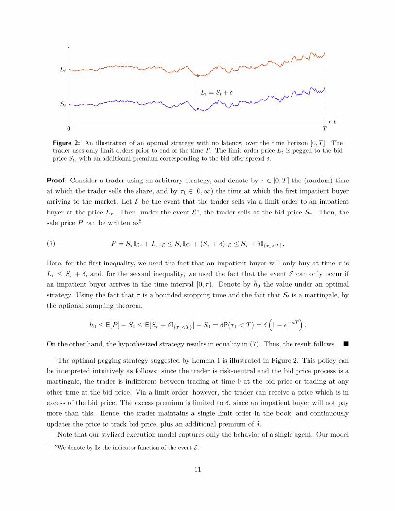
Figure 2: An illustration of an optimal strategy with no latency, over the time horizon [0, T ]. Thetrader uses only limit orders prior to end of the time T . The limit order price Lt is pegged to the bidprice St, with an additional premium corresponding to the bid-offer spread δ.
Proof. Consider a trader using an arbitrary strategy, and denote by τ ∈ [0, T ] the (random) timeat which the trader sells the share, and by τ1 ∈ [0,∞) the time at which the first impatient buyerarriving to the market. Let E be the event that the trader sells via a limit order to an impatientbuyer at the price Lτ . Then, under the event Ec, the trader sells at the bid price Sτ . Then, thesale price P can be written as8
P = Sτ IEc + Lτ IE ≤ Sτ IEc + (Sτ + δ)IE ≤ Sτ + δI{τ1<T}.(7)
Here, for the first inequality, we used the fact that an impatient buyer will only buy at time τ isLτ ≤ Sτ + δ, and, for the second inequality, we used the fact that the event E can only occur ifan impatient buyer arrives in the time interval [0, τ). Denote by h0 the value under an optimalstrategy. Using the fact that τ is a bounded stopping time and the fact that St is a martingale, bythe optional sampling theorem,
h0 ≤ E[P ]− S0 ≤ E[Sτ + δI{τ1<T}]− S0 = δP(τ1 < T ) = δ(1− e−µT
).
On the other hand, the hypothesized strategy results in equality in (7). Thus, the result follows. �
The optimal pegging strategy suggested by Lemma 1 is illustrated in Figure 2. This policy canbe interpreted intuitively as follows: since the trader is risk-neutral and the bid price process is amartingale, the trader is indifferent between trading at time 0 at the bid price or trading at anyother time at the bid price. Via a limit order, however, the trader can receive a price which is inexcess of the bid price. The excess premium is limited to δ, since an impatient buyer will not paymore than this. Hence, the trader maintains a single limit order in the book, and continuouslyupdates the price to track bid price, plus an additional premium of δ.
Note that our stylized execution model captures only the behavior of a single agent. Our model8We denote by IE the indicator function of the event E .
11
does not capture the strategic response of other agents, either competing agents submitting limitorders to sell, or contra-side impatient buyers. Both of these types of agents might be expected toreact to the activity of the limit order trader, and may diminish the gains of the limit order trader.Separately, our model also exaggerates the gains to be earned by placing limit orders rather thanmarket orders, due to the fact we do not include adverse selection costs incurred by limit orders.
However, at a high level, a trader in our model with a mandate to trade over a fixed time horizonbut with no private information as to the asset value prefers limit orders to market orders. Webelieve this is representative of the situation of algorithmic traders executing large “parent” ordersin practice. When executing a “child” order over a short time horizon, such traders typically firstsubmit limit orders, and then “clean up” with market orders as time runs short. Hence, despiteomissions of strategic considerations and other significant simplifications, the resulting policies docapture representative features of real world trading, if only at a stylized level. Moreover, oursimplified single-agent mode enables us to address the dynamic nature of trade execution andobtain a closed-form expression highlighting the exact drivers of the latency cost.
3. A Model for Latency
The optimal policy for the stylized execution problem of Section 2 relied on the ability of a trader tocontinuously track an informational process, namely, the bid price in the market, and to update hisorder as the process evolves. Here, we will consider a variation of that problem where the traderis unable to continuously participate in the market, but faces a fixed latency ∆t > 0.9 We areinterested in quantifying the cost of this latency by comparing the expected payoff in this model tothat in the stylized model without latency. Note that the model at hand is quite basic with regardsto some of primitives (e.g., the stochastic process describing the evolution of bid prices), we willdiscuss a number of tractable extensions in Section 4.4, including more complicated models of thebid price process and of limit order execution.
In general, latency that a trader experiences can take many forms. Minimally, for example,there is the delay of the data feeds that deliver market price information to the trader. There isthe delay of the trader’s own decision making. Finally, there is the delay of the trader’s resultingorder reaching the marketplace. We assume that the trader makes decisions instantaneously — wewill see that this is reasonable since the optimal decision rule for the trader will take a very simpleform. Further, from the trader’s perspective, the roundtrip delay (the total delay for an order tobe processed by an exchange and reflected in the data feeds observed by the trader) cannot bedecomposed into a delay to the exchange and a delay from the exchange. Hence, without loss of
9Note that many modern exchanges explicitly allow for pegged orders; these orders obviate the need for the traderto continually track the bid price in the manner we describe. However, more generally, when tracking an alternativeinformational process such as the price on a different exchange, the fundamental value (see Section 2), etc., a traderwould still need to continuously monitor the market relative to the informational process, and latency would beimportant.
12

T0 = 0 Ti = i∆t Ti+1 Ti+2 T = n∆t· · · · · ·
`i−1`i
`i+1
`0 `i `i+1 `i+2
Figure 3: An illustration of the model of latency. Here, the time horizon [0, T ] is divided into n slots,each of duration equal to the latency ∆t. The limit order price `i is decided at the start of the ithtime slot, i.e., at time Ti. This price only takes effect ∆t units of time later, and is active during thesubsequent time interval [Ti+1, Ti+2).
generality, we will assume that the trader is able to observe market price information with no delayor latency,10 but that the trader’s orders experience a latency ∆t before they are processed by theexchange. This latency is meant to capture, for example, networking or routing delays that arespecific to the trader, and that might be reduced through colocation or additional investment innetworking technology.
In our latency model, we consider an investor who maintains a limit order to sell one share overthe time horizon [0, T ] (the possibility of market orders will be discussed shortly), so that oncethe limit order is executed, the investor immediately exits the market. The time horizon [0, T ] isdivided into n slots each of length ∆t, i.e., T = n∆t. For each i ∈ {0, 1, . . . , n}, define Ti , i∆t.
At each time Ti, based on all information observed thus far, we assume that the trader caninstantaneously decide to update the limit order with a new price `i. Due to a latency of ∆t, theupdated price does not reach the market and take effect until the beginning of the next time slot,i.e., Ti+1. This limit order price remains active until time Ti+2, at which point it is superseded11
by the next price `i+1. This sequence of events is illustrated in Figure 3. Between the time Ti,when the price `i is decided, and the time Ti+1, when the updated order reaches the market, thefollowing events can occur:
• E(1)i : An impatient buyer arrives in the time interval (Ti, Ti+1) and `i−1 ≤ STi + δ, i.e., the
prior limit price `i−1, which is active at that time, is within a margin δ of the bid price at thestart of the interval. In this case, the limit order executes at the price `i−1, and the investorleaves the market. Note that the updated limit price `i never takes effect.
We assume that the probability that an impatient buyer arrives in any given time slot is µ∆t,and that these arrivals occur independently of everything else.12 We assume that ∆t < 1/µ
10Equivalently, we can assume that our definition of time corresponds to the trader’s clock.11In practice, this ordering scheme might be achieved by a sequence of cancel-and-replace limit orders, each of
which cancels the prior limit order, and inserts a new limit order with the updated price. If the prior limit order hasalready been filled when a subsequent cancel-and-replace order arrives, the new order will fail. Hence, the investor isguaranteed to sell at most one share.
12Note that this is simply a discrete-time Bernoulli arrival process that is analogous to the the Poisson arrivalprocess of Section 2.
13
so that this probability is well-defined. The bid price process evolves according to the randomwalk (2).
• E(2)i : Otherwise, if STi+1 ≥ `i, i.e., the bid price has crossed the order price `i at the instant
the order reaches the market, then the order immediately executes at price STi+1 .
• E(3)i : Otherwise, the limit order price `i is active over the time interval [Ti+1, Ti+2).
In order to consider the possibility of market orders, we allow the limit price `i = −∞. Bypicking this price, the trader can guarantee that the bid price at time Ti+1 will cross the order price,i.e., STi+1 ≥ `i with probability 1. Thus, the choice of `i = −∞ corresponds to a certain executionat the bid price STi+1 , i.e., a market order. Similarly, the trader can make the decision at time Tinot to trade by setting `i = ∞. As in the model of Section 2, if the investor has been unable tosell the share by the end of the time horizon T , the investor is forced to sell via a ‘clean-up’ trade,i.e., a market order at time T . This is accomplished by enforcing the constraint that `n−1 = −∞,which we will assume implicitly in what follows.
As before, if P is the random variable associated with the sale price, the trader is risk-neutraland seeks to solve the optimization problem
(8) h0(∆t) , maximize`0,...,`n−1
E [P ]− S0.
Here, the maximization is over the choice of limit order prices (`0, `1, . . . , `n−1). We assume thatthe price decisions are non-anticipating, i.e., each `i is adapted to the filtration generated by thebid price process and the arrival of impatient buyers up to and including time Ti. Our goal is toanalyze h0(∆t), which is the value under an optimal trading strategy when the latency is ∆t.
Note that, as compared to the model of Section 2, our present model with latency differs in twoways: First, the trader makes decisions at the beginning of discrete-time intervals of length ∆t, asopposed to continuously. Second, the orders of the trader incur a latency or delay of length ∆tbefore they reach the marketplace. We are interested in studying the impact of the latter feature,latency, and we adopt the former feature, discrete-time decision making, so as to admit a tractabledynamic programming analysis. In Section 4.3, however, we will see that in the low latency regimein which we are most interested, the discrete-time nature of our model has a negligible impact.
4. Analysis
In this section, we solve for the optimal policy for the trader in the latency model of Section 3. Thisproblem can be solved via a dynamic programming decomposition that is presented in Section 4.1.While the exact dynamic programming solution can be computed numerically, in Section 4.2 wewill present an asymptotic analysis that provides a closed-form analytic expression for the cost oflatency in the low latency regime, where ∆t→ 0. In Section 4.3, we will consider the implications
14

of the discrete-time nature of our latency model. Finally, in Section 4.4, we will discuss a numberof extensions of our latency model.
4.1. Dynamic Programming Decomposition
The standard approach to solving the optimal control problem (8) is to employ dynamic program-ming arguments. In Appendix A of the electronic companion, we formally derive the optimalcontrol policy using these methods. In order to focus on the high level picture, however, for themoment we will be content with summarizing those results.
In particular, assume a fixed latency of ∆t. For each decision time Ti with 0 ≤ i < n, define Uito be the event that the trader’s limit order remains unfulfilled prior to time Ti+1, i.e., none of theorders submitted at prices `0, . . . , `i−1 are executed. Note that if the event Ui does not hold, thenthe limit order price `i to be decided at time Ti is irrelevant. This is because, by the time thatorder arrives to the market, the trader would have already sold a share. Define the quantity
(9) hi , maximize`i,...,`n−1
E [P | STi , Ui]− STi .
Note that h0 = h0(∆t), where h0(∆t) is defined in (8), and thus our notation is consistent. Moregenerally, for i > 0, we can interpret hi to be the trader’s expected payoff at time Ti relative tothe current bid price STi under the optimal policy, the order does not get filled prior to time Ti+1.Thus, hi can be interpreted as a continuation value in the dynamic programming context.
The continuation values {hi} quantify the remaining value for a trader at each time period ifhis order remains unfulfilled. Given the continuation values, at each time Ti, the investor can makean optimal decision as to the limit order price `i by balancing the benefits of execution in the timeslot [Tt+1, Ti+2) with the value hi+1 that will be obtained if the order is not executed. Moreover,the optimal decisions and continuation values can be jointly computed via backward induction of aBellman equation. This result is captured in the following theorem. The proof, which is providedin Appendix A of the electronic companion, follows from formal dynamic programming arguments.
Theorem 1. Suppose {hi} satisfy, for 0 ≤ i < n− 1,
hi = maxui
{µ∆t
[ui
(Φ(
ui
σ√
∆t
)− Φ
(ui − δσ√
∆t
))+ σ√
∆t(φ
(ui
σ√
∆t
)− φ
(ui − δσ√
∆t
))]+hi+1
[(1− µ∆t)Φ
(ui
σ√
∆t
)+ µ∆tΦ
(ui − δσ√
∆t
)]},
(10)
and
(11) hn−1 = 0.
Here, φ and Φ are, respectively, the p.d.f. and c.d.f. of the standard normal distribution. Then,{hi} correspond to the continuation values under the optimal policy.
15
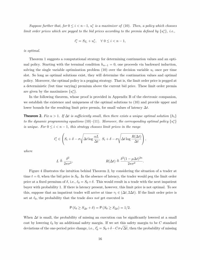
Suppose further that, for 0 ≤ i < n−1, u∗i is a maximizer of (10). Then, a policy which chooseslimit order prices which are pegged to the bid prices according to the premia defined by {u∗i }, i.e.,
`∗i = STi + u∗i , ∀ 0 ≤ i < n− 1,
is optimal.
Theorem 1 suggests a computational strategy for determining continuation values and an opti-mal policy. Starting with the terminal condition hn−1 = 0, one proceeds via backward induction,solving the single variable optimization problem (10) over the decision variable ui once per timeslot. So long as optimal solutions exist, they will determine the continuation values and optimalpolicy. Moreover, the optimal policy is a pegging strategy. That is, the limit order price is pegged ata deterministic (but time varying) premium above the current bid price. These limit order premiaare given by the maximizers {u∗i }.
In the following theorem, whose proof is provided in Appendix B of the electronic companion,we establish the existence and uniqueness of the optimal solutions to (10) and provide upper andlower bounds for the resulting limit price premia, for small values of latency ∆t.
Theorem 2. Fix α > 1. If ∆t is sufficiently small, then there exists a unique optimal solution {hi}to the dynamic programming equations (10)–(11). Moreover, the corresponding optimal policy {u∗i }is unique. For 0 ≤ i < n− 1, this strategy chooses limit prices in the range
`∗i ∈
Si + δ − σ
√∆t log αL∆t , Si + δ − σ
√∆t log R(∆t)
∆t
,where
L ,δ2
2πσ2 , R(∆t) , δ2(1− µ∆t)2n
2πσ2 .
Figure 4 illustrates the intuition behind Theorem 2, by considering the situation of a trader attime t = 0, when the bid price is S0. In the absence of latency, the trader would peg the limit orderprice at a fixed premium of δ, i.e., `0 = S0 +δ. This would result in a trade with the next impatientbuyer with probability 1. If there is latency present, however, this limit price is not optimal. To seethis, suppose that an impatient trader will arrive at time τ1 ∈ (∆t, 2∆t). If the limit order price isset at `0, the probability that the trade does not get executed is
P (`0 ≥ S∆t + δ) = P (S0 ≥ S∆t) = 1/2.
When ∆t is small, the probability of missing an execution can be significantly lowered at a smallcost by lowering `0 by an additional safety margin. If we set this safety margin to be C standarddeviations of the one-period price change, i.e., `′0 = S0 +δ−Cσ
√∆t, then the probability of missing
16

t0 ∆t 2∆tτ1
S0
S0 + σ√
∆t
S0 − σ√
∆t
`0 S0 + δ
`′0 S0 + δ − Cσ√
∆t
`∗0 S0 + u∗0
Figure 4: An illustration of the optimal policy of Theorem 2. In the absence of latency, at time t = 0,the trader would set the limit price at a premium of δ, i.e., `0 = S0 + δ. In an environment with latency,the trader might set the limit price to be `′0, which lowers `0 by an additional safety margin of Cstandard deviations. This serves to increase the likelihood of trade execution in the interval (∆t, 2∆t).The optimal limit price `∗0 utilizes a safety margin that is slightly larger.
execution becomes
P(`′0 ≥ S∆t + δ
)= P
(S0 − Cσ
√∆t ≥ S∆t
)= Φ(−C).
This probability can be made close to 0 by the choice of C. However, given a fixed choice of Cindependent of ∆t, the probability remains constant (i.e., independent of ∆t) and non-zero. Theadditional safety margin corresponding to the log term in Theorem 2 is a second order adjustment.This is introduced so that, given the optimal limit price `∗0, the probability of execution tends to 1as ∆t→ 0.
4.2. Asymptotic Analysis
The dynamic programming decomposition developed in Section 4.1 allows the exact numericalcomputation of the value h0(∆t), the value under an optimal policy of the latency model introducedin Section 3, when the latency is ∆t. As discussed earlier, the latency observed in modern electronicmarkets is extremely small, often on the time scale of milliseconds. Thus, we are most interested inthe qualitative behavior of h0(∆t) in the asymptotic regime where ∆t→ 0. The main result of thissection is the following theorem, whose proof is provided in Appendix C of the electronic companion.It provides a closed-form expression for h0(∆t), which holds asymptotically13 as ∆t→ 0.
13In what follows, given arbitrary functions f and g, and a positive function q, we will say that f(∆t) =g(∆t) + O(q(∆t)) if lim sup∆t→0 |f(∆t) − g(∆t)|/q(∆t) < ∞, i.e., if the difference between f and g, as ∆t → 0,is asymptotically bounded above by some positive multiple of q. Similarly, we will say that f(∆t) = g(∆t)+o(q(∆t))
17
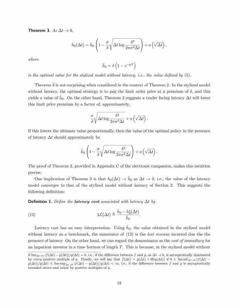
Theorem 3. As ∆t→ 0,
h0(∆t) = h0
1− σ
δ
√∆t log δ2
2πσ2∆t
+ o(√
∆t),
whereh0 = δ
(1− e−µT
)is the optimal value for the stylized model without latency, i.e., the value defined by (5).
Theorem 3 is not surprising when considered in the context of Theorem 2. In the stylized modelwithout latency, the optimal strategy is to peg the limit order price at a premium of δ, and thisyields a value of h0. On the other hand, Theorem 2 suggests a trader facing latency ∆t will lowerthis limit price premium by a factor of, approximately,
σ
δ
√∆t log δ2
2πσ2∆t + o(√
∆t).
If this lowers the ultimate value proportionally, then the value of the optimal policy in the presenceof latency ∆t should approximately be
h0
1− σ
δ
√∆t log δ2
2πσ2∆t
+ o(√
∆t).
The proof of Theorem 3, provided in Appendix C of the electronic companion, makes this intuitionprecise.
One implication of Theorem 3 is that h0(∆t) → h0 as ∆t → 0, i.e., the value of the latencymodel converges to that of the stylized model without latency of Section 2. This suggests thefollowing definition:
Definition 1. Define the latency cost associated with latency ∆t by
(12) LC(∆t) , h0 − h∗0(∆t)h0
.
Latency cost has an easy interpretation. Using h0, the value obtained in the stylized modelwithout latency as a benchmark, the numerator of (12) is the lost revenue incurred due the thepresence of latency. On the other hand, we can regard the denominator as the cost of immediacy foran impatient investor in a time horizon of length T . This is because, in the stylized model without
if lim∆t→0 |f(∆t)− g(∆t)|/q(∆t) = 0, i.e., if the difference between f and g, as ∆t→ 0, is asymptotically dominatedby every positive multiple of q. Finally, we will say that f(∆t) = g(∆t) + Θ(q(∆t)) if 0 < lim inf∆t→0 |f(∆t) −g(∆t)|/q(∆t) ≤ lim sup∆t→0 |f(∆t) − g(∆t)|/q(∆t) < ∞, i.e., if the difference between f and g is asymptoticallybounded above and below by positive multiples of q.
18
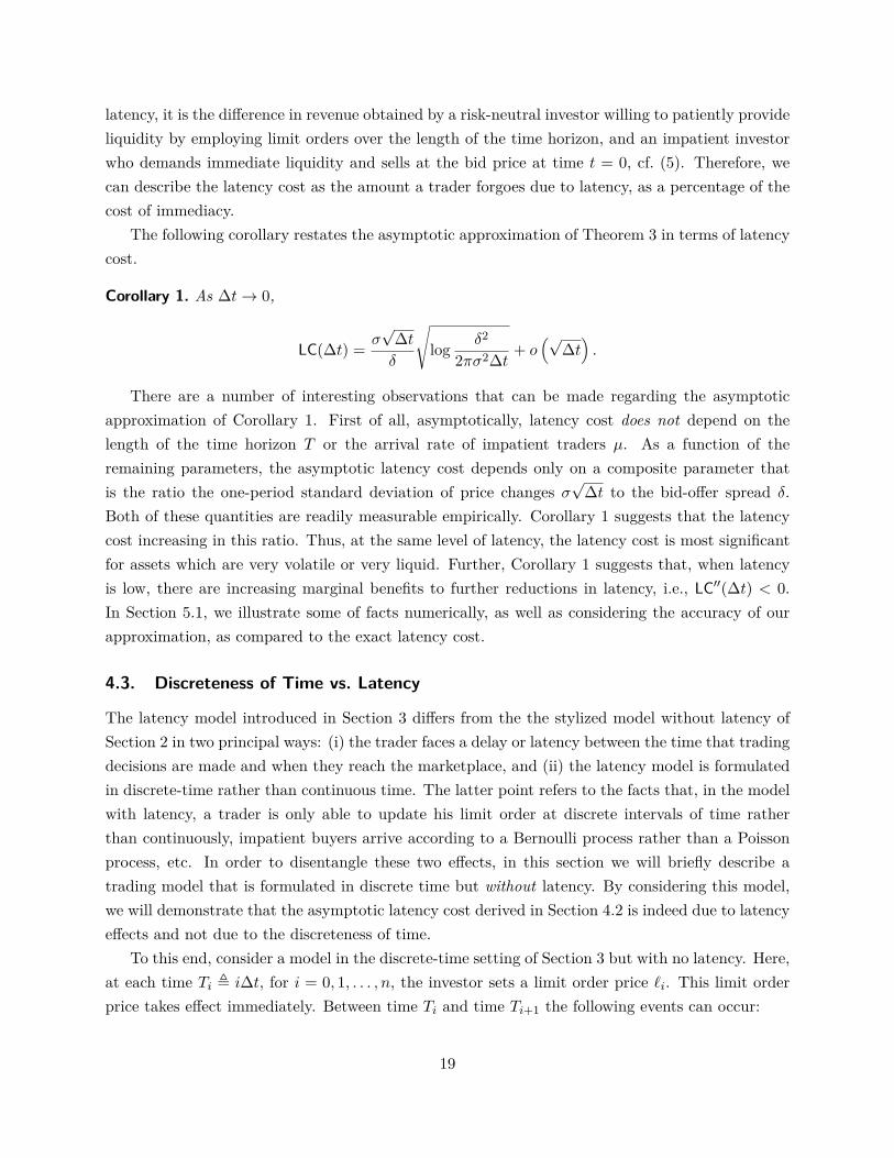
latency, it is the difference in revenue obtained by a risk-neutral investor willing to patiently provideliquidity by employing limit orders over the length of the time horizon, and an impatient investorwho demands immediate liquidity and sells at the bid price at time t = 0, cf. (5). Therefore, wecan describe the latency cost as the amount a trader forgoes due to latency, as a percentage of thecost of immediacy.
The following corollary restates the asymptotic approximation of Theorem 3 in terms of latencycost.
Corollary 1. As ∆t→ 0,
LC(∆t) = σ√
∆tδ
√log δ2
2πσ2∆t + o(√
∆t).
There are a number of interesting observations that can be made regarding the asymptoticapproximation of Corollary 1. First of all, asymptotically, latency cost does not depend on thelength of the time horizon T or the arrival rate of impatient traders µ. As a function of theremaining parameters, the asymptotic latency cost depends only on a composite parameter thatis the ratio the one-period standard deviation of price changes σ
√∆t to the bid-offer spread δ.
Both of these quantities are readily measurable empirically. Corollary 1 suggests that the latencycost increasing in this ratio. Thus, at the same level of latency, the latency cost is most significantfor assets which are very volatile or very liquid. Further, Corollary 1 suggests that, when latencyis low, there are increasing marginal benefits to further reductions in latency, i.e., LC′′(∆t) < 0.In Section 5.1, we illustrate some of facts numerically, as well as considering the accuracy of ourapproximation, as compared to the exact latency cost.
4.3. Discreteness of Time vs. Latency
The latency model introduced in Section 3 differs from the the stylized model without latency ofSection 2 in two principal ways: (i) the trader faces a delay or latency between the time that tradingdecisions are made and when they reach the marketplace, and (ii) the latency model is formulatedin discrete-time rather than continuous time. The latter point refers to the facts that, in the modelwith latency, a trader is only able to update his limit order at discrete intervals of time ratherthan continuously, impatient buyers arrive according to a Bernoulli process rather than a Poissonprocess, etc. In order to disentangle these two effects, in this section we will briefly describe atrading model that is formulated in discrete time but without latency. By considering this model,we will demonstrate that the asymptotic latency cost derived in Section 4.2 is indeed due to latencyeffects and not due to the discreteness of time.
To this end, consider a model in the discrete-time setting of Section 3 but with no latency. Here,at each time Ti , i∆t, for i = 0, 1, . . . , n, the investor sets a limit order price `i. This limit orderprice takes effect immediately. Between time Ti and time Ti+1 the following events can occur:
19

• If STi ≤ `i, i.e., the bid price is less than the limit order price, the limit order immediatelyexecutes at the price STi .
• Otherwise, suppose that an impatient buyer arrives in the time interval (Ti, Ti+1) and `i ≤STi + δ, i.e., the limit price `i is within a margin δ of the bid price at the start of the interval.In this case, the limit order executes at the price `i. We assume that an impatient buyerarrives with probability µ∆t, independent of everything else.
As before, if the investor is unable to sell the share by the end of the time interval, he is forced tosell via a market order, i.e., `n = −∞. If P is the sale price, the optimal value for the trader inthis discrete model is given by
hD0 (∆t) , maximize
`0,...,`nE [P ]− S0.
We have the following result, whose proof is identical to the martingale argument used to establishLemma 1.
Lemma 2. An optimal strategy for the discrete model is to place limit orders at the price `i = STi +δ,for i = 0, 1, . . . , n− 1. This strategy achieves the value
hD0 (∆t) , δ
(1− (1− µ∆t)n
).
Now, note that, for all 0 < ∆t < 1/µ,
e−µT−12µ
2T∆t ≤ (1− µ∆t)T/∆t ≤ e−µT .
Therefore, the difference in value between the continuous model of Section 2 and the discrete modelconsidered here is at most
∣∣hD0 (∆t)− h0
∣∣ ≤ δe−µT (1− e−12µ
2T∆t)≤ 1
2δµ2Te−µT∆t.
In other words, this difference is asymptotically O(∆t). By Theorem 3, however, the differencebetween the continuous model and the latency model is asymptotically
Θ(√
∆t log(1/∆t)).
Hence, the asymptotic effect of latency dominates the asymptotic effect of the discreteness of time.
4.4. Extensions
The analysis of the latency model that we have presented proceeded according to two high levelsteps:
20
(i) First, in Section 4.1, a simplified dynamic programming decomposition was developed. Inthis decomposition, at each time, the trader’s value function is parameterized by a singlescalar, rather than being an arbitrary function of state. This allows the Bellman equation tobe solved through a system of n equations in n unknowns, given by (10)–(11).
(ii) Second, in Section 4.2, an asymptotic analysis of the simplified dynamic programming equa-tions (10)–(11) was performed. This gave rise to the asymptotic latency cost expression ofCorollary 1.
The dynamic programming decomposition step (i) that is at the heart of our analysis can beextended to a much broader set of stochastic primitives than the present setting. In each of thesecases, a different set of simplified dynamic programming equations, analogous to (10)–(11) wouldarise, and would require a customized variation of asymptotic analysis step (ii). In particular,consider the following tractable generalizations:
• Price process. In our model, the price process St is a Brownian motion. Our dynamicprogramming decomposition only requires that the St be a Markov process and a martin-gale. It would be straightforward to extend the dynamic programming step (i) and con-sider other Markovian martingales, for example, allowing for non-Gaussian processes, time-inhomogeneous volatility, or for jump processes.
On the other hand, the asymptotic analysis step (ii) we have presented is quite sensitiveto distributional assumptions of the price process, and would require specialized analysisfor any such generalization. In Appendix D of the electronic companion, we consider onegeneralization of particular interest, where the price dynamics also contain a jump component.
• Limit order execution. In our model, the execution of a limit order in the time slot(Ti, Ti+1) required that the limit order price `i−1 be within a spread δ of the bid price STi ,and that an impatient trader arrive. More generally, our dynamic programming decomposi-tion only requires that the execution of this limit order, conditional on the price difference`i−1 − STi , be independent of everything else. This can accommodate a number of general-izations, for example, the arrival rate of impatient buyers can be time-varying. Further, themaximum premium above the bid price St that an impatient buyer is willing to pay can berandomly distributed, as in (3). This would allow models where a limit order that is pricedaggressively low has a much higher probability of execution. Such models could alternativelybe interpreted, as discussed in Section 2, as cases where the prevailing bid-offer spread is notconstant, but is independent and identically distributed, varying from period to period.
5. Empirical Estimation of Latency Cost
In this section, we will consider empirical applications of our model. First, we will illustratethe optimal trading policy and the corresponding value function when the model parameters are
21

estimated from high frequency market data for a single stock. We will also compare the exactlatency cost (numerically computed via dynamic programming) to the approximation provided byCorollary 1 in order to access the quality of our approximation. Subsequently, we show the historicalevolution of latency cost and implied latency across a range of U.S. equities using cross-sectionaldata on volatilities and bid-offer spreads during the 1995–2005 period.
Our empirical analysis should be regarded as a first-order study to obtain a rough calibration ofour model. It will allow us to analyze the model in relevant parameter regimes, as well as gaininga broad understanding the implications of our model for the trading of U.S. equities. Under ourmodeling assumptions (e.g., Browian motion price processes, Poisson arrivals of impatient traders,constant bid-offer spread, etc.), our empirical measurement of latency cost requires estimates of thehigh frequency price volatility σ and the prevailing bid-offer spread δ. Here, we make a number ofsimplifications and rely on the recent empirical work of Aït-Sahalia and Yu (2009) to obtain thesequantities:
• We estimate price volatility σ using the maximum likelihood estimates of the volatility ofreturns provided by Aït-Sahalia and Yu (2009). Note that this estimation of high frequencyvolatility aims to filter out the impact of microstructure noise and obtain an unbiased estimateof daily volatility. However, for an investor with a trading horizon of 1 second, microstructurenoise needs to be incorporated as well. Therefore, the high frequency volatility estimate thatis used in our empirical analysis underestimates the actual volatility faced by a high frequencytrader with a very short trading horizon.
• Recall that the prevailing bid-offer spread, δ, equals the bid-offer spread in the absence ofthe liquidating trader. In the empirical data, it is impossible to disentangle the presence ofliquidating traders. Moreover, the bid-offer spread will not be constant, but will vary overthe course of the trading day. As a proxy for δ, we use the average bid-offer spread over thetrading day.
Despite these shortcomings, we believe that our empirical analysis can shed light on the importanceof latency in the trading of U.S. equities.
5.1. The Optimal Policy and the Approximation Quality
In what follows, we will numerically evaluate the optimal policy in our model, the correspondingvalue function, and the latency cost approximation. These numerical experiments are meant tobe illustrative of our model. We will use realistic model parameters estimated from recent marketdata for a single stock. Our methodology here is not meant to be authoritative — there aremany subtleties in the analysis of high frequency data; these are beyond the scope of the work athand. However, we do seek to demonstrate that our model parameters can be readily derived fromcommonly available data.
22
Specifically, the model parameters herein are estimated from trade-and-quote (TAQ) data for astock that is a representative example of a liquid name, Goldman Sachs Group, Inc. (NYSE: GS),on the trading day of January 4, 2010. This data was obtained from the Wharton Research andData Services (WRDS) consolidated TAQ database. Only trades and quotes originating from theprimary exchange (NYSE) during regular trading hours were considered. The model parameterswere estimated as follows:
• Initial bid price: SGS0 = $170.00. This was chosen to be the first transaction price on the
trading day.
• Bid-offer spread: δGS = $0.058, i.e., equivalently, 3.4 basis points relative to the initial priceSGS
0 . This was estimated by computing the average spread between bid and offer quotes overthe course of the trading day and rounding to the nearest cent.
• Arrival rate of market orders: µGS = 12.03 (per minute). This was estimated by dividing thetotal number of NYSE trades by the length of the trading day.
• Price volatility: σGS = $1.92 (daily), i.e., approximately equivalent to an annualized volatilityof returns of 17.9%. These were estimated from the time series of transaction prices over thecourse of the trading day, using maximum likelihood estimation as described inAït-Sahaliaand Yu (2009).
• Trading horizon: T = 10 (seconds).
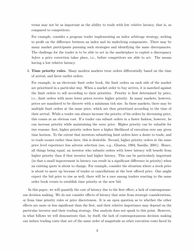
Figure 5 illustrates the optimal limit order policy for GS under different values of latency. Ifthere is no latency, the limit orders are submitted at a constant premium of δ. When there islatency, the optimal order policy is obtained using the exact dynamic programming solution of(10)–(11). As the latency increases, the limit order premium is reduced below δ so as to accountfor the increasing uncertainty of price movements over the latency interval. Theorem 2 suggeststhat this reduction is approximately equal to
(13) σ
√∆t log δ2
2πσ2∆t .
In Figure 5, we see that, with a latency of 500 ms, this adjustment is up to approximately 1.4σ√
∆t,i.e., 1.4 times the standard deviation of prices over the latency interval. When the latency is reducedto 250 ms and to 50 ms, the adjustment increases to 1.6 and 2.1 standard deviations, respectively.The fact that this adjustment, when measured as a multiple of the uncertainty over the latencyperiod, increases as the latency decreases is consistent with (13).
In Figure 5, we also observe that as t increases and the trading deadline approaches, the limitorder premium u∗t becomes lower. This makes intuitive sense: the trader faced with a terminalvalue of 0 since he is required to sell using market order at the end of the period. As the deadline
23

0 1 2 3 4 5 6 7 8 9 100.04
0.05
0.06
0
δ
δ − 2.1σ√
∆t1
δ − 1.6σ√
∆t2
δ − 1.4σ√
∆t3
Time t (sec)
Lim
itpr
ice
prem
iumu∗ t
=`∗ t−St
($)
∆t0 = 0 (ms)∆t1 = 50 (ms)∆t2 = 250 (ms)∆t3 = 500 (ms)
Figure 5: An illustration of the optimal strategy for GS, expressed in terms of limit price premiumover the course of the time, for different choices of latency. In each case, the dashed line illustrates therelative distance below the bid-offer spread δ of the price premium of the final limit order, as a multipleof the standard deviation of prices over the latency interval.
approaches, the trader is more willing to sacrifice the potential profits of a limit order in order toincrease the probability of execution.
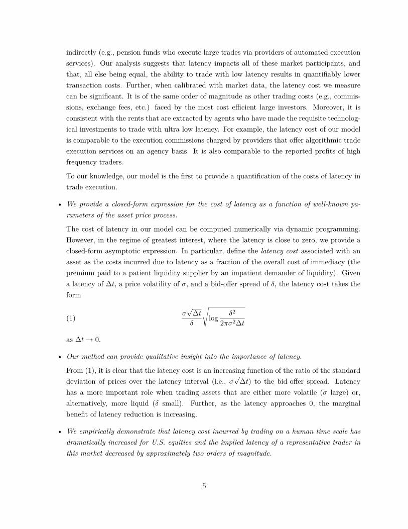
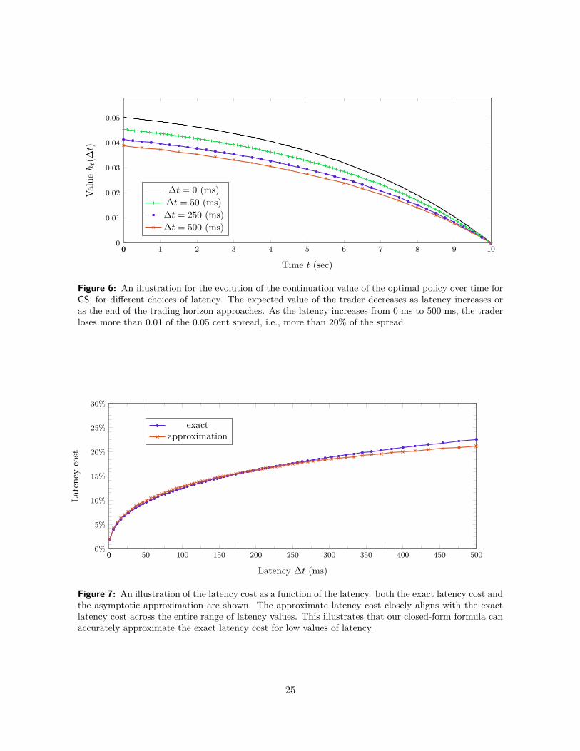
Figure 6 illustrates the corresponding continuation value under the optimal policy for GS, fordifferent values of latency. Clearly, the trader’s expected payoff decreases as latency increases orthe end of the trading horizon approaches.
Finally, Figure 7 illustrates the latency cost as a function of latency. Both the exact value ofthe latency cost, computed numerically via the dynamic programming decomposition (10)–(11),and the asymptotic latency cost approximation provided by Corollary 1 are shown. The latencycosts decrease from approximately 20% of the cost of immediacy to 5% of the cost of immediacy,as the latency decreases from 500 ms to 5 ms. Further, the marginal benefit of reducing latencyincreases as the latency approaches zero. Finally, we note that the approximate and exact latencycosts are quite close across the entire range of latency values. This suggests that the approximationis of very high quality in this case.
5.2. Historical Evolution of Latency Cost
In this section, we will examine the historical evolution of latency cost in U.S. equities. Here, weconsider the situation of a hypothetical investor with a fixed latency of 500 milliseconds. Thischoice of latency is made approximately to reflect the reaction time of a very fast human trader.We will use this as a proxy for the fastest possible trading on a “human time scale”. By analyzing
24
0 1 2 3 4 5 6 7 8 9 100
0.01
0.02
0.03
0.04
0.05
0
Time t (sec)
Valu
eht(∆t)
∆t = 0 (ms)∆t = 50 (ms)∆t = 250 (ms)∆t = 500 (ms)
Figure 6: An illustration for the evolution of the continuation value of the optimal policy over time forGS, for different choices of latency. The expected value of the trader decreases as latency increases oras the end of the trading horizon approaches. As the latency increases from 0 ms to 500 ms, the traderloses more than 0.01 of the 0.05 cent spread, i.e., more than 20% of the spread.
0 50 100 150 200 250 300 350 400 450 5000%
5%
10%
15%
20%
25%
30%
0
Latency ∆t (ms)
Late
ncy
cost
exactapproximation
Figure 7: An illustration of the latency cost as a function of the latency. both the exact latency cost andthe asymptotic approximation are shown. The approximate latency cost closely aligns with the exactlatency cost across the entire range of latency values. This illustrates that our closed-form formula canaccurately approximate the exact latency cost for low values of latency.
25

the evolution of the associated latency cost, we will get a sense of the importance of latency overtime.
Our empirical analysis relies on the data set of Aït-Sahalia and Yu (2009). Their data setcontains estimates for various liquidity measures for all NYSE common stocks on a daily basis duringthe sample period of June 1, 1995 to December 31, 2005. The estimates are derived from intradaytransaction prices and quotes from the NYSE TAQ database. We utilized only the volatility andbid-offer spread data as we have seen both analytically (Corollary 1) and numerically (Figure 7)that, under our modeling assumptions, latency cost can be approximated accurately for low valuesof latency using only these two measures.
The data set contain volatility and bid-offer spread estimates for given stock on a particularday if the number of transactions on that day exceeds 200. The minimum, average, and maximumnumber of stocks in the sample on any day are 61, 653, and 1,278, respectively. In particular, earlierperiods in the data set contain fewer stocks due to a smaller number of firms and a lower volumeof transactions. In this data set, the bid-offer spread is estimated using only NYSE quotes in theregular trading hours. The volatility estimate is obtained using maximum likelihood estimation inthe presence of market microstructure noise. Maximum likelihood estimation is preferred over othernonparametric estimation methods (e.g., “Two Scales Realized Volatility”) as a simulation studyshows that maximum likelihood estimation provides robust estimators under reasonable stochasticvolatility and jump models in the underlying asset. The reader is urged to consult to Section 2.1of Aït-Sahalia and Yu (2009) for full details of their estimation procedure.
For each stock in the data set, on a daily basis, we compute the latency cost facing an investorwith a fixed latency of 500 ms using the asymptotic approximation of Corollary 1. These dailylatency costs are then averaged over each month. Figure 8 displays percentiles of the monthlyaverages of latency cost over all of the stocks in the sample, as a function of time. As a representativeexample of a liquid name, we also report the monthly averages of latency cost of Goldman SachsGroup, Inc. (NYSE: GS). Note that the time series for GS begins from its initial public offering in1999. For reference, we have added an additional point to this time series based on our estimationin Section 5.1 of the latency cost for GS on January 4, 2010.
Figure 8 illustrates that latency costs have had an increasing trend over the 1995–2005 period.In particular, we observe that the median latency cost incurred by trading on a human time scaleroughly tripled, by increasing from approximately 5% to approximately 14%. One important factorin this increase has been the reduction of bid-offer spreads over this time period. Instances duringthe period when the NYSE reduced the tick size (from $1/8 to $1/16 in June 1997, and from $1/16 to$0.01 in January 2001) coincide with spikes in latency cost. This is consistent with bid-offer spreadsdecreasing significantly and volatility maintaining the same level at these times. This suggests thatany future reduction in tick sizes will result in increased latency costs.
Using a data set in a similar time-frame, from February 2001 to December 2005, Hendershottet al. (2010) conclude that in the post-decimalization era, the increase in algorithmic trading activity
26

1995 1996 1997 1998 1999 2000 2001 2002 2003 2004 2005 2006 2007 2008 2009 20100%
5%
10%
15%
20%
25%
$1/8 tick size $1/16 tick size $0.01 tick size
Year
Late
ncy
cost
(mon
thly
aver
age)
,∆t
=50
0(m
s)
90th percentile75th percentile
median25th percentile
GS
Figure 8: An illustration of the historical evolution of latency cost over the 1995–2005 time period.Here, we consider a hypothetical “human time scale” investor with a fixed latency of ∆t = 500 (ms).Percentiles for the resulting latency cost are reported across NYSE common stocks. The latency costsare computed from data set of Aït-Sahalia and Yu (2009). The latency cost for GS is also reported,beginning from its IPO. The dashed lines correspond to dates where the NYSE tick size was reduced.We observe that latency cost had a consistent increasing trend over the 1995–2005 period. Specifically,the median latency cost approximately increased three-fold by reaching roughly to 14% from 5%.
27
had a positive impact on the level of liquidity. This result suggests that the increase in algorithmictrading in and of itself elevated the importance of low latency trading and increased the cost oflatency.
5.3. Historical Evolution of Implied Latency
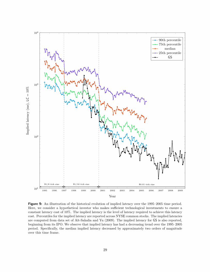
An alternative perspective on the historical importance of latency comes from considering a hypo-thetical investor with a target level for the cost of latency, relative to the overall cost-of-immediacy.The representative trader maintains this target over time through continual technological upgradesto lower levels of latency. We determine the requisite level of latency for such a trader, over timeand across the aggregate market. In other words, fixing the latency cost percentage LC to thetarget level, we can solve the asymptotic approximation (12) for the level of latency required ateach time to achieve latency cost LC. We call this the implied latency.
Figure 9 illustrates the implied latency values over the 1995–2005 period assuming that thetarget level LC = 10% of overall transaction costs result from latency. We observe that the medianimplied latency decreased by approximately two orders of magnitude over this time frame. The90th percentile of U.S. equities, for example, went from an implied latency on the scale of secondsto an implied latency on the scale of tens of milliseconds.
5.4. Empirical Importance of Latency
Our model captures the cost of latency due to a lack of contemporaneous information. Figure 8suggests that, when our model is calibrated to the topmost quartile of U.S. equities, a investorwith latency on the human time scale faces a latency cost of at 15% to 25%. In order to assess thesignificance of this, we can compare it to other trading costs. Suppose we normalize the cost ofimmediacy to $0.01, which is the typical bid-offer spread for a liquid U.S. equity. Then, our modelsuggests that the benefit of reducing latency from a human time scale of 500 ms to an ultra lowlatency time scale of less than 1 ms is approximately $0.0015–$0.0025 per share traded.
While this might seem very small as an absolute number, note that is of the same order of mag-nitude as other trading costs faced by the most cost efficient institutional investors. For example,a hedge fund would pay an average commission of $0.0007 per share for market access.14 Further-more, investors may pay an SEC fee of $0.0005 per share traded,15 and exchange fees or rebatesof $0.0020–$0.0030 per share traded. To the extent that a sophisticated institutional investor iscost sensitive and wishes to optimize these other execution costs, they should also be concernedwith latency. This isn’t to suggest that latency cost is important to all investors. A typical retail
14“U.S. Equity Trading: Low Touch Trends,” TABB Group, July 2010.15As of January 21, 2011, the SEC fee is a fraction $0.0000192 of the proceeds of an equity sale. If we assume a
typical stock price of $50, this is approximately $0.0010 per share sold. Amortizing this cost equally between buysand sells results in $0.0005 per share traded.
28
1995 1996 1997 1998 1999 2000 2001 2002 2003 2004 2005 2006 2007 2008 2009101
102
103
104
$1/8 tick size $1/16 tick size $0.01 tick size
Year
Impl
ied
late
ncy
(ms)
,LC
=10
%
90th percentile75th percentile
median25th percentile
GS
Figure 9: An illustration of the historical evolution of implied latency over the 1995–2005 time period.Here, we consider a hypothetical investor who makes sufficient technological investments to ensure aconstant latency cost of 10%. The implied latency is the level of latency required to achieve this latencycost. Percentiles for the implied latency are reported across NYSE common stocks. The implied latenciesare computed from data set of Aït-Sahalia and Yu (2009). The implied latency for GS is also reported,beginning from its IPO. We observe that implied latency has had a decreasing trend over the 1995–2005period. Specifically, the median implied latency decreased by approximately two orders of magnitudeover this time frame.
29

investor, for example, may pay a brokerage fee that is up to $0.10 per share traded.16 For thislatter type of investor, the cost of latency as described here is not a significant component of overalltrading costs.
Alternatively, we can compare the $0.0015–$0.0025 per share traded latency cost to the rentsextracted by agents that have made the required technological investments to trade on an ultra lowlatency time scale. For example, providers of automated algorithmic trade execution services chargean average commission of $0.0033 per share traded for their execution services, which leveragesophisticated low latency technological infrastructure.17 Note that this cost is comparable to thelatency cost. Another class of agents with ultra low latency trading capabilities are high frequencytraders. Reported net profit numbers for high frequency traders are in the range of $0.0010–$0.0020per share traded.18 This is of the same order of magnitude as the latency cost.
6. Conclusion and Future Directions
This paper provides a model to quantify the cost of latency on transaction costs. We considera stylized execution problem, where a trader must sell an atomic unit of stock over a fixed timehorizon. We consider this model in the absence of latency as a benchmark, and we incorporatelatency by not allowing the trader to continuously participate in the market. Orders submittedby the trader reach the market with a fixed latency, and the trader is forced to deviate from thebenchmark policy in order to take into account the uncertainty introduced by this delay. Wequantify the cost of latency as the normalized difference in expected payoffs between this modeland the stylized model without latency.
Since the latency values observed in modern electronic markets are on the order of milliseconds,we provide an asymptotic analysis for the low latency regime, in which we obtain an explicitclosed-form solution. In order to compute this asymptotic latency cost empirically, we only needto estimate the volatility and the average bid-offer spread of the stock. This is an elegant andpractical result as data sets and estimation procedures for these quantities are readily abundantin the literature. Indeed, using an existing data set, we show that the cost of latency incurred bytrading on a human time scale (500 ms) increased three-fold over the 1995–2005 time-frame. Inaddition, using the alternative approach of keeping a fixed level of latency cost through continuoustechnological improvements, we compute the various percentiles of the implied latency over thistime frame. Using the same data set, we observe that the median implied latency decreased byapproximately two orders of magnitude.
16For example, at the time of writing, the brokerage firm E-TRADE charges $10 per trade. Assuming a typicaltrade of 100 shares, this cost is $0.10 per share traded.
17“U.S. Equity Trading: Low Touch Trends,” TABB Group, July 2010. Note that some institutional investors paysignificantly larger commissions for trade execution in order to compensate their brokers for trading ideas or researchservices. The commission we quote here is for “non-idea driven” services that relate purely to trade execution usingthe algorithms and technological platform of the broker.
18“Tradeworx, Inc. Public Commentary on SEC Market Structure Concept Release,” Tradeworx, Inc., April 2010.
30
Our empirical analysis can also be utilized to compare the magnitude of latency cost to othertrading costs incurred by institutional investors. Our results suggest that the difference in payoffbetween trading with a human time scale (500 ms) and an automated trading platform with ultralow latency (1 ms) is approximately of the same order of magnitude as other trading costs facedby institutional investors. This observation certainly underlines the significance of latency for suchinvestors. In conclusion, our model is the first theoretical approach in the literature to concretelyquantify the impact of latency on the optimal order submission policy and its resulting cost to thetrader.
There are a number of interesting future directions for research. First, as discussed in Sec-tion 4.4, there are a number of tractable extensions to the present model that can be analyzed.More generally, in the introduction, we identified a number of broad themes to the costs that arisefrom latency. The model we have presented captures mainly costs due to a lack of contemporaneousdecision making. It does not capture the latency costs due to strategic effects (i.e., comparativeadvantage/disadvantage relative to other investors) or due to time priority rules. These remainimportant questions for future research.
ReferencesY. Aït-Sahalia and J. Jacod. Is Brownian motion necessary to model high-frequency data? The Annals of
Statistics, 38(5):3093–3128, 2010.
Y. Aït-Sahalia and J. Yu. High frequency market microstructure noise estimates and liquidity measures.The Annals of Applied Statistics, 3(1):422–457, 2009.
R. Almgren and N. Chriss. Optimal execution of portfolio transactions. Journal of Risk, 3:5–40, 2001.
J. Angel. Limit versus market orders. Working Paper No. FINC-1377-01-293, School of Business Adminis-tration, Georgetown University, Washington, D.C., 1994.
J. Bacidore, R. Battalio, and R. Jennings. Order submission strategies, liquidity supply, and trading inpennies on the New York Stock Exchange. Journal of Financial Markets, 6:337–362, 2003.
K. Back and S. Baruch. Working orders in limit order markets and floor exchanges. The Journal of Finance,62(4):1589–1621, 2007.
O. E. Barndorff-Nielsen, D. G. Pollard, and N. Shephard. Discrete-valued Lévy processes and low latencyfinancial econometrics. Working paper, 2010.
D. P. Bertsekas and S. E. Shreve. Stochastic Optimal Control: The Discrete Time Case. Academic Press,Orlando, 1978.
D. Bertsimas and A. Lo. Optimal control of execution costs. Journal of Financial Markets, 1(1):1–50, 1998.
D. Bertsimas, L. Kogan, and A. W. Lo. When is time continuous? Journal of Financial Economics, 55:173–204, 2000.
P. P. Boyle and D. Emanuel. Discretely adjusted option hedges. Journal of Financial Economics, 8:259–282,1980.
J. Brogaard. High frequency trading and its impact on market quality. Working paper, 2010.
31

G. Cespa and T. Foucault. Insiders-outsiders, transparency, and the value of the ticker. Working Paper No.628, Department of Economics, Queen Mary, University of London, April 2008.
G. C. Chacko, J. W. Jurek, and E. Stafford. The price of immediacy. Journal of Finance, 63(3):1253–1290,2008.
S.N. Cohen and L. Szpruch. A limit order book model for latency arbitrage. Arxiv preprint arXiv:1110.4811,2011.
T. Copeland and D. Galai. Information effects and the bid-ask spread. Journal of Finance, 38(5):1457–1469,1983.
J. Cvitanic and A. Kirilenko. High frequency traders and asset prices. Working paper, March 2010.
R. Durrett. Probability: Theory and Examples. Duxbury Press, 3rd edition, 2004.
D. Easley, T. Hendershott, and T. Ramadorai. The price of latency. Working paper, May 2008.
L. R. Glosten. Is the electronic open limit order book inevitable? Journal of Finance, 49(4):1127–1161,1994.
S. Grossman and M. Miller. Liquidity and market structure. Journal of Finance, 43:617–633, 1988.
L. Harris. Optimal dynamic order submission strategies in some stylized trading problems. FinancialMarkets, Institutions & Instruments, 7(2):1–76, April 1998.
J. Hasbrouck. Empirical Market Microstructure. Oxford University Press, 2007.
J. Hasbrouck and G. Saar. Technology and liquidity provision: The blurring of traditional definitions.Journal of Financial Markets, 12:143–172, 2009.
J. Hasbrouck and G. Saar. Low-latency trading. Working paper, 2010.
T. Hendershott and R. Riordan. Algorithmic trading and information. Working paper, September 2009.
T. Hendershott, C. M. Jones, and A. Menkveld. Does algorithmic trading improve liquidity? To appear inJournal of Finance, April 2010.
R. A. Jarrow and P. Protter. A dysfunctional role of high frequency trading in electronic markets. Workingpaper, 2011.
A. Kirilenko, A. Kyle, M. Samadi, and T. Tuzun. The flash crash: The impact of high frequency trading onan electronic market. Working paper, 2010.
H. Leland. Option pricing and replication with transactions costs. Journal of Finance, 40:1283–1301, 1985.
A. W. Lo, A. C. MacKinlay, and J. Zhang. Econometric models of limit order execution. Journal of FinancialEconomics, 65:31–71, 2002.
E. Pagnotta. Information and liquidity trading at optimal frequencies. Technical report, Working paper,NYU Stern, 2010.
C.A. Parlour and D.J. Seppi. Limit order markets: A survey. Handbook of Financial Intermediation andBanking, 5, 2008.
A. F. Perold. The implementation shortfall: Paper versus reality. Journal of Portfolio Management, 14(3):4–9, 1988.
32

M. J. Ready. The specialist’s discretion: Stopped orders and price improvement. Review of Financial Studies,12(5):1075–112, Winter 1999.
R. Roll. A simple implicit measure of the effective bid-ask spread in an efficient market. Journal of Finance,39:1127–1139, 1984.
P. Sandås. Adverse selection and competitive market making: Empirical evidence from a limit order market.Review of Financial Studies, 14(3):705–734, 2001.
H. R. Stoll and C. Schenzler. Trades outside the quotes: Reporting delay, trading option or trade size?Journal of Financial Economics, 79:615–653, 2006.
I. Werner. NYSE order flow, spreads, and information. Journal of Financial Markets, 6:309–335, 2003.
Ciamac C. Moallemi is the Barbara and Meyer Feldberg Associate Professor of Businessin the Decision, Risk, and Operations Division of the Graduate School of Business at ColumbiaUniversity. His research interests are in the area of the optimization and control of large-scalestochastic systems, with an emphasis on applications in financial engineering and the design offinancial markets.
Mehmet Saglam is currently a Postdoctoral Research Associate at Bendheim Center for Fi-nance, Princeton University. His research is broadly focused on optimal (or near-optimal) dynamicdecision-making in high-dimensional stochastic systems. He is particularly interested in financialapplications with market frictions arising from transaction costs, illiquidity, and trading infrastruc-ture.
33

Electronic Companion to “The Cost of Latency inHigh-Frequency Trading”
Ciamac C. MoallemiGraduate School of Business
Columbia Universityemail: [email protected]
Mehmet SaglamBendheim Center for Finance
Princeton Universityemail: [email protected]
Current Revision: February 5, 2013
A. Dynamic Programming Decomposition
In order to solve the optimal control problem (8) via dynamic programming, note that we canequivalently consider the objective of maximizing the sale price P . Consider a decision time Tiwith 0 ≤ i < n, and assume that the trader’s limit order remains unfilled at time Ti. The state ofthe system consists of the current price, STi as well as the previously chosen limit price,1 `i−1, sincethis price will become active at time Ti. We can define an optimal value function Ji(STi , `i−1), asa function of this state, by optimizing the eventual sale price over all future decisions. In otherwords,
(A.1) Ji(STi , `i−1) , maximize`i,...,`n−1
E [P | STi , `i−1] .
At time T = Tn, the trader must sell via a market order, hence
(A.2) Jn(STn , `n−1) = STn .
Now, for 0 ≤ i < n, there are three mutually exclusive events one of which must occur betweentime Ti and time Ti+1. These are the events E(1)
i , E(2)i , and E(3)
i described in Section 3. Byconsidering cases corresponding to these events, we have the Bellman equation
(A.3) Ji(STi , `i−1) , max`i
E[IE(1)
i
`i−1 + IE(2)i
STi+1 + IE(3)i
Ji+1(STi+1 , `i)∣∣∣∣ STi , `i−1
].
Here, the first term corresponds to an execution at the prior price `i−1, the second term correspondsto the price `i being crossed by the bid price upon arrival to the market, and the third termcorresponds to all other cases.
Define the function Qi, for 0 ≤ i ≤ n, by
Qi(STi , vi−1) , Ji(STi , STi + vi−1)− STi .
1We will assume that `−1 =∞, i.e., there is no limit order active at the beginning of the time horizon.
1
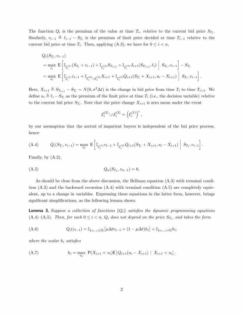
The function Qi is the premium of the value at time Ti, relative to the current bid price STi .Similarly, vi−1 , `i−1 − STi is the premium of limit price decided at time Ti−1 relative to thecurrent bid price at time Ti. Then, applying (A.3), we have for 0 ≤ i < n,
Qi(STi , vi−1)
= max`i
E[IE(1)
i
(STi + vi−1) + IE(2)i
STi+1 + IE(3)i
Ji+1(STi+1 , `i)∣∣∣∣ STi , vi−1
]− STi
= maxui
E[IE(1)
i
vi−1 + IE(2)i ∪E
(3)i
Xi+1 + IE(3)i
Qi+1(STi +Xi+1, ui −Xi+1)∣∣∣∣ STi , vi−1
].
Here, Xi+1 , STi+1 − STi ∼ N(0, σ2∆t) is the change in bid price from time Ti to time Ti+1. Wedefine ui , `i−STi as the premium of the limit price at time Ti (i.e., the decision variable) relativeto the current bid price STi . Note that the price change Xi+1 is zero mean under the event
E(2)i ∪ E
(3)i =
(E(1)i
)c,
by our assumption that the arrival of impatient buyers is independent of the bid price process,hence
(A.4) Qi(STi , vi−1) = maxui
E[IE(1)
i
vi−1 + IE(3)i
Qi+1(STi +Xi+1, ui −Xi+1)∣∣∣∣ STi , vi−1
].
Finally, by (A.2),
(A.5) Qn(STn , vn−1) = 0.
As should be clear from the above discussion, the Bellman equation (A.3) with terminal condi-tion (A.2) and the backward recursion (A.4) with terminal condition (A.5) are completely equiv-alent, up to a change in variables. Expressing these equations in the latter form, however, bringssignificant simplifications, as the following lemma shows.
Lemma 3. Suppose a collection of functions {Qi} satisfies the dynamic programming equations(A.4)–(A.5). Then, for each 0 ≤ i < n, Qi does not depend on the price STi, and takes the form
(A.6) Qi(vi−1) = I{vi−1≤δ}[µ∆tvi−1 + (1− µ∆t)hi
]+ I{vi−1>δ}hi,
where the scalar hi satisfies
(A.7) hi = maxui
P(Xi+1 < ui)E [Qi+1(ui −Xi+1) | Xi+1 < ui] .
2

Proof. Observe that, for 0 ≤ i < n, (A.4) can be simplified according to
Qi(STi , vi−1)
= maxui
µ∆tvi−1I{vi−1≤δ}
+(1− µ∆tvi−1I{vi−1≤δ}
)E[I{Xi+1<ui}Qi+1(STi +Xi+1, ui −Xi+1)
∣∣∣ STi
],
(A.8)
where we have used the definitions of the events E(1)i and and E(3)
i .Now, we proceed by backward induction. For the terminal case i = n− 1, from (A.8) and the
fact that Qn = 0 and un−1 = −∞ (i.e., the trader must use a market order at the last time slot),we have that
Qn−1(STn−1 , vn−2) = µ∆tvn−2I{vn−2≤δ}.
In other words, Qn−1 satisfies the hypotheses of the lemma, with hn−1 = 0.Now, suppose that the result holds for some 0 ≤ i+ 1 < n. By (A.8), and since Qi+1 does not
depend on STi+1 ,
Qi(STi , vi−1)
= maxui
µ∆tvi−1I{vi−1≤δ} +(1− µ∆tvi−1I{vi−1≤δ}
)E[I{Xi+1<ui}Qi+1(ui −Xi+1)
]= µ∆tvi−1I{vi−1≤δ} +
(1− µ∆tvi−1I{vi−1≤δ}
)hi
= I{vi−1≤δ}[µ∆tvi−1 + (1− µ∆tvi−1)hi
]+ I{vi−1>δ}hi.
Here, in the second equality, we define hi through (A.7). The result then follows. �
Notice that, at the beginning of the trading horizon, there is no active limit order, i.e., u−1 =∞.From Lemma 3, we have that
h0 = Q0(∞) = maximize`0,...,`n−1
E [P | S0]− S0.
In other words, h0 = h0(∆t), as defined in (8), and our notation is consistent. More generally, fori > 0, from (A.7), we can interpret hi to be the trader’s expected payoff at time Ti relative to thecurrent bid price under the optimal policy, assuming that the limit order does not get executed inthat time slot. Thus, hi can be interpreted as a continuation value in the dynamic programmingcontext, as in (9).
The continuation values {hi} allow for a compact representation of the value function, sincethey consist of only a single real number for each time slot, rather than a function of the entire statespace. Theorem 1 directly expresses the dynamic programming equations (A.4)–(A.5) in terms ofthis representation. The proof follows by explicitly computing the expectations in Lemma 3.
3

Theorem 1. Suppose {hi} satisfy, for 0 ≤ i < n− 1,
hi = maxui
{µ∆t
[ui
(Φ(
ui
σ√
∆t
)− Φ
(ui − δσ√
∆t
))+ σ√
∆t(φ
(ui
σ√
∆t
)− φ
(ui − δσ√
∆t
))]+hi+1
[(1− µ∆t)Φ
(ui
σ√
∆t
)+ µ∆tΦ
(ui − δσ√
∆t
)]},
(A.9)
and
(A.10) hn−1 = 0.
Here, φ and Φ are, respectively, the p.d.f. and c.d.f. of the standard normal distribution. Then, {hi}correspond to the continuation values under the optimal policy. In other words, the value functions{Qi} defined by {hi} via (A.6) solve the dynamic programming equations (A.4)–(A.5).
Suppose further that, for 0 ≤ i < n − 1, u∗i is a maximizer of (A.9). Then, a policy whichchooses limit prices according to the premia defined by {u∗i }, i.e.,
`∗i = STi + u∗i , ∀ 0 ≤ i < n− 1,
is optimal.
Proof. Suppose that we are given {hi} that satisfy the hypotheses of the theorem. Define {Qi} bysetting, for 0 ≤ i ≤ n− 1,
(A.11) Qi(vi−1) , I{vi−1≤δ}[µ∆tvi−1 + (1− µ∆t)hi
]+ I{vi−1>δ}hi,
and Qn , 0. We wish to show that {Qi} solve the dynamic programming equations (A.4)–(A.5).Note that (A.5) holds by definition. For 0 ≤ i < n, we have that (A.4) is equivalent to (A.8).
Define Qi to be the right side of (A.8), i.e.,
Qi(vi−1) , µ∆tvi−1I{vi−1≤δ} +(1− µ∆tvi−1I{vi−1≤δ}
)maxui
E[I{Xi+1<ui}Qi+1(ui −Xi+1)
].
Comparing with (A.11), in order that the dynamic programming equation (A.8) hold (i.e., thatQi = Qi), we must have that
(A.12) hi = maxui
E[I{Xi+1<ui}Qi+1(ui −Xi+1)
]Using the definition of Qi+1 from (A.11), this is equivalent to
hi
= maxui
E[I{Xi+1<ui}
(I{ui−Xi+1≤δ}
[µ∆t(ui −Xi+1) + (1− µ∆t)hi+1
]+ I{ui−Xi+1>δ}hi+1
)]= max
uiE[I{0<ui−Xi+1≤δ}µ∆t(ui −Xi+1) + I{Xi+1<ui}(1− µ∆t)hi+1 + I{ui−Xi+1>δ}µ∆thi+1
].
4

For the first term in the expectation, we have
E[I{0<ui−Xi+1≤δ}µ∆t(ui −Xi+1)
]= µ∆t
∫ ui
−∞(ui − x)I{ui−x≤δ}
1σ√
∆tφ
(x
σ√
∆t
)dx
= µ∆t∫ ui
ui−δ(ui − x) 1
σ√
∆tφ
(x
σ√
∆t
)dx
= µ∆t[ui
(Φ(
ui
σ√
∆t
)− Φ
(ui − δσ√
∆t
))+∫ ui
ui−δ
−xσ√
∆tφ
(x
σ√
∆t
)dx
]= µ∆t
[ui
(Φ(
ui
σ√
∆t
)− Φ
(ui − δσ√
∆t
))+ σ√
∆t(φ
(ui
σ√
∆t
)− φ
(ui − δσ√
∆t
))].
For the second term in the expectation, we have
E[I{Xi+1<ui}(1− µ∆t)hi+1
]= (1− µ∆t)hi+1Φ
(ui
σ√
∆t
).
finally, for the last term in the expectation, we have
E[I{ui−Xi+1>δ}µ∆thi+1
]= µ∆thi+1Φ
(ui − δσ√
∆t
)Combining all the terms, we obtain the desired recursion for hi.
The balance of the theorem involves establishing the optimality of the {u∗i } policy. This followsfrom standard dynamic programming arguments (see, e.g., Chapter 3, Bertsekas and Shreve, 1978).
�
B. Proof of Theorem 2
We begin with a preliminary lemma.
Lemma 4. Suppose that {hi : 0 ≤ i < n} solves the dynamic programming recursion (10)–(11).Then, for 0 ≤ i < n,
(B.1) 0 ≤ hi ≤ δ(1− (1− µ∆t)n
)< δ.
Proof. First, note that the result is trivially true for i = n−1, since hn−1 = 0. Now, if 0 ≤ i < n−1,we can always choose ui = −∞, i.e., a market order, and this results in a continuation value of 0.Thus, hi ≥ 0.
For the upper bound, consider the discrete model without latency described in Section 4.3.Any strategy for the latency model is also feasible for the discrete model, since the trader cansimply delay the implementation of trading decisions by one period. Therefore, at time Ti (with0 ≤ i < n − 1), a policy with latency cannot achieve more value than the optimal policy for the
5
discrete model without latency. At time Ti, there are n − i − 1 trading decisions remaining. Thiscorresponds to the initial time of a discrete model with a total time horizon of (n− i−1)∆t. Then,with reference to Lemma 2, we have that
hi ≤ δ(1− (1− µ∆t)n−i−1).
The result immediately follows. �
Theorem 2. Fix α > 1. If ∆t is sufficiently small, then there exists a unique optimal solution {hi}to the dynamic programming equations (10)–(11). Moreover, the corresponding optimal policy {u∗i }is unique. For 0 ≤ i < n− 1, this strategy chooses limit prices in the range
`∗i ∈
Si + δ − σ
√∆t log αL∆t , Si + δ − σ
√∆t log R(∆t)
∆t ,
,where
L ,δ2
2πσ2 , R(∆t) , δ2(1− µ∆t)2n
2πσ2 .
Proof. Assume that, for some 0 ≤ i < n− 1, a solution {hj : i+ 1 ≤ j < n} exists to (10)–(11).We will establish that, for ∆t sufficiently small (and not dependent on i), a solution hi also existsand satisfies the conditions of the theorem. The result will follow by backward induction. Notethat the base case of our induction (i.e., the existence of hn−1) is trivial.
To this end, define the auxiliary function f by
f(u, h) , µ∆t[u(Φ(Au)− Φ(Bu)
)+ σ√
∆t(φ(Au)− φ(Bu)
)]+ h
[(1− µ∆t)Φ(Au) + µ∆tΦ(Bu)
],
(B.2)
where
Au ,u
σ√
∆t, Bu ,
u− δσ√
∆t.(B.3)
Then, from Theorem 1, for 0 ≤ i < n− 1, the dynamic programming recursion is given by
(B.4) hi = maxui
f(ui, hi+1),
and we can establish the present theorem by proving that, for ∆t sufficiently small, (B.4) has aunique maximizer u∗i ∈ (uL, uR), where
uL , δ − σ
√∆t log αL∆t , uR , δ − σ
√∆t log R(∆t)
∆t .(B.5)
6

Note that
(B.6) R(0) , lim∆t→0
R(∆t) = lim∆t→0
L(1− µ∆t)2T/dt = Le−2µT < αL.
Hence, there exists some ∆t > 0 so that if 0 < ∆t < ∆t, then
δ/2 < uL < uR < δ, and 0 < 1− µ∆t < 1.
For the balance of the theorem, we will assume that 0 < ∆t < ∆t, in addition to whatever otherassumptions are made regarding the magnitude of ∆t.
The first and second derivatives of f(·, h) are given by
fu(u, h) = µ∆t[Φ(Au)− Φ(Bu) +Au
(φ(Au)− φ(Bu)
)− uφ(Au) + (δ − u)φ(Bu)
σ√
∆t
]+ h
σ√
∆t
[(1− µ∆t)φ(Au) + µ∆tφ(Bu)
]= (1− µ∆t)h
σ√
∆tφ(Au) + µ∆t
[Φ(Au)− Φ(Bu)− δ
σ√
∆tφ(Bu)
]+ hµ
√∆t
σφ(Bu)
= (1− µ∆t)hσ√
∆tφ(Au) + µ∆t
[Φ(Au)− Φ(Bu)
]+ µ√
∆tσ
φ(Bu)(h− δ),
fuu(u, h) = −u(1− µ∆t)hσ3∆t
√∆t
φ(Au) + µ√
∆tσ
[φ(Au)− φ(Bu)
]+ µ(δ − u)
σ3√
∆tφ(Bu)(h− δ)
= φ(Au)[µ√
∆tσ− u(1− µ∆t)h
σ3∆t3/2
]+ φ(Bu)
[µ(δ − u)σ3√
∆t(h− δ)− µ
√∆tσ
].
(B.7)
First, we will show that, for ∆t sufficiently small, f(·, hi+1) has a local maximum u∗i in theinterval (uL, uR), and that this is the unique maximizer over the larger interval (δ/2, δ). That is,u ∈ (δ/2, δ) and u 6= u∗i , then
(B.8) f(u, hi+1) < f(u∗i , hi+1), for all u ∈ (δ/2, δ), u 6= u∗i .
This is implied by the following claims, which we will demonstrate hold for ∆t sufficiently small:
(i) fu(uL, hi+1) > 0.
(ii) fu(uR, hi+1) < 0.
(iii) fuu(u, hi+1) < 0, for all u ∈ (δ/2, δ).
7

Claim (i): Note that
fu(uL, hi+1) = (1− µ∆t)hi+1
σ√
∆tφ(AuL
) + µ∆t[Φ(AuL
)− Φ(BuL)]
+ µ∆tδ√α
(hi+1 − δ)
≥ µ∆t[Φ(AuL
)− Φ(BuL)]− µ∆t√
α,
(B.9)
where we use the fact that hi+1 ≥ 0 (cf. Lemma 4). In order to calculate a lower bound forΦ(AuL
) − Φ(BuL), we need the following standard bound on the tail probabilities of the normal
distribution (see, e.g., Durrett, 2004). Define Q to be the tail probability of a standard normaldistribution, i.e.,
Q(x) , 1− Φ(x) = 1√2π
∫ ∞x
e−12u
2du.
Then, for all x > 0,
(B.10) x2 − 1x3√
2πe−
12x
2≤ Q(x) ≤ 1
x√
2πe−
12x
2.
Applying this to (B.9),
fu(uL, hi+1) ≥ µ∆t[1−Q(AuL
)−Q(−BuL)]
+ µ∆t√α
= µ∆t(
1− 1√α
)− µ∆t
[Q(AuL
) +Q(−BuL)]
> µ∆t(
1− 1√α
)− 2µ∆tQ(−BuL
)
≥ µ∆t(
1− 1√α
)− 2µ∆t3/2√
2παL log αL∆t
> 0,
for sufficiently small ∆t. Here, we have used the fact that Q(−BuL) > Q(AuL
).
8

Claim (ii): Similarly, for the other endpoint of the interval, we have
fu(uR, hi+1) = (1− µ∆t)hi+1
σ√
∆tφ(AuR
) + µ∆t[1−Q(AuR
)−Q(−BuR)]
+ µ∆tδ(1− µ∆t)n (hi+1 − δ)
≤ (1− µ∆t)hi+1
σ√
∆tφ(AuR
) + µ∆t[1−Q(AuR
)−Q(−BuR)]
+ µ∆tδ(1− µ∆t)n [δ (1− (1− µ∆t)n)− δ]
= (1− µ∆t)hi+1
σ√
∆tφ(AuR
) + µ∆t[1−Q(AuR
)−Q(−BuR)]− µ∆t
= (1− µ∆t)hi+1
σ√
∆tφ(AuR
)− µ∆t[Q(AuR
) +Q(−BuR)]
≤ δ
σ√
∆tφ(AuR
)− µ∆tQ(−BuR),
where we have used the upper bound on hi+1 from Lemma 4. Using (B.6), for sufficiently small∆t, we have √
log R(∆t)∆t <
δ
2σ√
∆t,
and thusAuR
≥ δ
2σ√
∆t.
On the other hand, using (B.10),
Q(−BuR) ≥
[(log R(∆t)
∆t
)−1/2−(
log R(∆t)∆t
)−3/2]√ ∆t2πR(∆t) .
Thus,
fu(uR, hi+1) ≤ δ
σ√
2π∆texp
(−δ2
8σ2∆t
)
− µ∆t[(
log R(∆t)∆t
)−1/2−(
log R(∆t)∆t
)−3/2]√ ∆t2πR(∆t)
< 0,
for sufficiently small ∆t.
Claim (iii): Note that, for u ∈ (δ/2, δ),
φ
(δ
σ√
∆t
)< φ(Au) < φ
(δ
2σ√
∆t
)< φ(Bu) < φ(0).
9
Then, from (B.7), and using the fact that 0 ≤ hi+1 < δ (cf. Lemma 4), we have for ∆t sufficientlysmall,
fuu(u, hi+1) ≤ φ(Au)µ√
∆tσ
+ φ(Bu)[µ(δ − u)σ3√
∆t(hi+1 − δ)−
µ√
∆tσ
]
≤ φ(Bu)µ(δ − u)σ3√
∆t(hi+1 − δ) < 0.
In order to complete the proof, it suffices to demonstrate that the local maximum u∗i ∈ (uL, uR)is the unique global maximum. Since u∗i achieves a higher value than any other u ∈ (δ/2, δ), wewill analyze cases where u /∈ (δ/2, δ) as follows:
• u ∈ [0, δ/2].
Here,φ
(δ
σ√
∆t
)≤ φ(Bu) ≤ φ
(δ
2σ√
∆t
)≤ φ(Au) ≤ φ(0).
Further, for ∆t sufficiently small,
Φ(Au)− Φ(Bu) ≥ Φ (0)− Φ( −δ
2σ√
∆t
)≥ 1
4 .
Then, for ∆t sufficiently small,
fu(u, hi+1) ≥ (1− µ∆t)hi+1
σ√
∆tφ
(δ
2σ√
∆t
)+ µ∆t
[Φ (0)− Φ
( −δ2σ√
∆t
)]+ µ√
∆tσ
φ
(δ
2σ√
∆t
)(hi+1 − δ)
≥ hi+1
σ√
∆tφ
(δ
2σ√
∆t
)+ µ∆t
[Φ (0)− Φ
( −δ2σ√
∆t
)]− δµ
√∆t
σφ
(δ
2σ√
∆t
)≥ µ∆t
4 − µδ√
∆t√2πσ
exp(−δ2
8σ2∆t
)> 0.
(B.11)
Here, we have used the fact that hi+1 ≥ 0. Using (B.8) and the fact that f(·, hi+1) iscontinuous, this implies that
(B.12) supu∈[0,δ/2]
f(u, hi+1) ≤ f(δ/2, hi+1) < f(u∗i , hi+1).
• u ∈ (−∞, 0).
10
In this case, since hi+1 ≥ 0 and Bu < Au < 0,
fu(u, hi+1) ≥ µ∆t [Φ(Au)− Φ(Bu)]− δµ√
∆tσ
φ(Bu)
= µ∆t∫ Au
Bu
φ(z) dz − δµ√
∆tσ
φ(Bu)
> µ∆t(Au −Bu)φ(Bu)− δµ√
∆tσ
φ(Bu) = 0.
In conjunction with (B.12), this implies that
(B.13) supu∈(−∞,0)
f(u, hi+1) ≤ f(0, hi+1) < f(u∗i , hi+1).
• u ∈ [δ,∞).
In this case, using the upper bound on hi+1 from Lemma 4,
fu(u, hi+1) ≤ δ
σ√
∆tφ(Au) + µ∆t [Φ(Au)− Φ(Bu)]
− µδ(1− µ∆t)n√
∆tσ
φ(Bu).(B.14)
Consider two cases. First, assume that u > δ +√
∆t. Then, applying (B.10),
fu(u, hi+1) ≤ δ
σ√
∆tφ(Au) + µ∆tQ(Bu)− µδ(1− µ∆t)n
√∆t
σφ(Bu)
≤ δ
σ√
∆tφ(Au) + µσ∆t3/2
u− δφ(Bu)− µδ(1− µ∆t)n
√∆t
σφ(Bu)
≤ φ(Bu)[
δ
σ√
∆texp
(−δ2
2σ2∆t
)+ µσ∆t− µδ(1− µ∆t)n
√∆t
σ
].
Note that (1− µ∆t)n → e−µT as ∆t→ 0. Then, for ∆t sufficiently small,
(B.15) 12e−µT < (1− µ∆t)n.
Hence, for ∆t sufficiently small,
fu(u, hi+1) ≤ φ(Bu)[
δ
σ√
∆texp
(−δ2
2σ2∆t
)+ µσ∆t− µδe−µT
√∆t
2σ
]< 0.
On the other hand, suppose that u ∈ [δ, δ +√
∆t]. Then, from (B.14), (B.15), and since
11

0 < Bu < Au, we have for ∆t sufficiently small,
fu(u, hi+1) ≤ δ
σ√
∆tφ(Au) + µ∆t
2 − µδ(1− µ∆t)n√
∆tσ
φ(Bu)
≤ δ
σ√
∆tφ(Au) + µ∆t
2 − µδe−µT√
∆t2σ φ(Bu)
≤ δ
σ√
2π∆texp
(− δ2
2σ2∆t
)+ µ∆t
2 − µδe−µT√
∆t2σ√
2πexp
(− 1
2σ2
)< 0.
The above discussion, combined with (B.8) and the fact that f(·, hi+1) is continuous, impliesthat
(B.16) supu∈[δ,∞)
f(u, hi+1) ≤ f(δ, hi+1) < f(u∗i , hi+1).
�
C. Proof of Theorem 3
We will establish Theorem 3 via a sequence of lemmas. First, recall the function f(u, h) defined in(B.2) and the quantities uL and uR defined in (B.5).
Lemma 5. (i) As ∆t→ 0,
maxu∈[uL,uR]0≤i<n−1
|fuu(u, hi+1)| = O
(√∆t log 1
∆t
).
(ii) For all h ∈ R and ∆t sufficiently small,
0 ≤ fh(uR, h) ≤ 1.
Proof. We begin with (i). Recall Au and Bu from (B.3). Let u be in the interval [uL, uR]. Then,for 0 ≤ i < n− 1, from (B.7),
|fuu(u, hi+1)| ≤∣∣∣∣∣φ(Au)
[µ√
∆tσ− u(1− µ∆t)hi+1
σ3∆t3/2
]+ φ(Bu)
[µ(δ − u)σ3√
∆t(hi+1 − δ)−
µ√
∆tσ
]∣∣∣∣∣≤ φ(Au)µ
√∆tσ
+ φ(Au) δ2
σ3∆t3/2+ φ
(δ − uσ√
∆t
)[δµ(δ − u)σ3√
∆t+ µ√
∆tσ
].
Here, we have used the fact that 0 ≤ u ≤ δ and 0 ≤ hi+1 < δ (cf. Lemma 4). Note that, for ∆t
12

sufficiently small, uL ≥ δ/2. Then,
maxu∈[uL,uR]
φ(Au) ≤ φ(Aδ/2) = 1√2π
exp(− δ2
8σ2∆t
)≤ c0∆t2,
for an appropriately chosen constant c0. Thus,
|fuu(u, hi+1)| ≤ c0µ
σ∆t5/4 + c0δ
2
σ3
√∆t+ φ
(δ − uσ√
∆t
)[δµ(δ − u)σ3√
∆t+ µ√
∆tσ
]
≤ c0µ
σ∆t5/4 + c0δ
2
σ3
√∆t+ φ
(δ − uRσ√
∆t
)[δµ(δ − uL)σ3√
∆t+ µ√
∆tσ
]
= c0µ
σ∆t5/4 + c0δ
2
σ3
√∆t+
√∆t
2πR(∆t)
δµσ2
√log αL∆t + µ
√∆tσ
≤ c0µ
σ∆t5/4 + c0δ
2
σ3
√∆t+ µ∆t
σ√
2πR(∆t)+ δµ
σ2√
2πR(∆t)
√∆t log αL∆t .
Since R(∆t)→ Le−2µT as ∆t→ 0, the last term asymptotically dominates and (i) follows.For (ii), note that Φ(AuR
),Φ(BuR) ∈ (0, 1), so if ∆t < 1/µ, then for all h,
fh(uR, h) = (1− µ∆t)Φ(AuR) + µ∆tΦ(BuR
) ∈ (0, 1).
�
Lemma 6. As ∆t→ 0,
uR − uL = O
(√∆t
log 1∆t
).
Proof. Note that
uR − uL = σ√
∆t
√log αL∆t −
√log R(∆t)
∆t
= σ√
∆t[g(αL)− g
(R(∆t)
)],
where g(x) ,√
log x∆t . Then, by mean value theorem, for some z ∈
[R(∆t), αL
],
uR − uL = σ√
∆tg′(z)[αL−R(∆t)
]= σ
2z[αL−R(∆t)
]√ ∆tlog z
∆t≤ σαL
2R(∆t)
√√√√ ∆tlog R(∆t)
∆t.
The result follows since R(∆t)→ R(0) , Le−2µT as ∆t→ 0. �
Let {hi : 0 ≤ i < n − 1} be the optimal solution to the dynamic programming recursion(10)–(11), and let {u∗i : 0 ≤ i < n− 1} define the corresponding optimal policy. Define {hi : 0 ≤
13

i ≤ n− 1} by the recursion
hi ,
f(uR, hi+1) if 0 ≤ i < n− 1,
0 if i = n− 1.
Note that hi is the continuation value of the suboptimal policy that always chooses ui = uR, for0 ≤ i < n− 1. We are interested in quantifying its difference to the optimal continuation value.
Lemma 7. As ∆t→ 0,
0 ≤ h0 − h0 = O
(√∆t
log 1∆t
).
Proof. For 0 ≤ i < n− 1, define ∆i , hi − hi. Clearly, ∆i ≥ 0.Using the mean value theorem,
∆i = f(u∗i , hi+1)− f(uR, hi+1)
=[f(u∗i , hi+1)− f(uR, hi+1)
]+[f(uR, hi+1)− f(uR, hi+1)
]= −1
2fuu(u, hi+1)(uR − u∗i )2 + fh(uR, h)∆i+1.
where u is some point on the interval (u∗i , uR) and h is some point on the interval (hi+1, hi+1). Here,we have used the fact that the optimal solution u∗i satisfies the first order condition fu(u∗i , hi+1) = 0.
Using Lemmas 5 and 6, for ∆t sufficiently small, there exist constants c1 and c2 so that
maxu∈[uL,uR]0≤i<n−1
|fuu(u, hi+1)| ≤ c1
√∆t log 1
∆t , uR − uL ≤ c2
√∆t
log 1∆t.
Also, from Lemma 5, note that 0 ≤ fh(uR, h) ≤ 1. Then, we obtain that, for ∆t sufficiently small,
∆i ≤c1(uR − u∗i )2
2
√∆t log 1
∆t + ∆i+1 ≤c1c2
2∆t3/2√log 1
∆t
+ ∆i+1.
Then, since ∆n−1 = 0, we have that
∆0 ≤(T
∆t
)c1c2
2∆t3/2√log 1
∆t
= c1c2T
2
√∆t
log 1∆t.
�
Define the sequence {βi : 0 ≤ i ≤ n− 1} by the linear recursion
(C.1) βi ,
µ∆t(uR − βi+1) + βi+1 if 0 ≤ i < n− 1,
0 if i = n− 1.
14

Here, βi is an approximation to the value hi. The next lemma bounds the approximation error.
Lemma 8. As ∆t→ 0,
|h0 − β0| = O
(√∆t
log 1∆t
).
Proof. For 0 ≤ i < n − 1, define εi , hi − βi. Recall the following definition from the proof ofTheorem 2,
AuR,
uR
σ√
∆t, BuR
,uR − δσ√
∆t= −
√log R(∆t)
∆t .
Then, by the recursive definitions of hi and βi, 0 ≤ i < n− 1,
εi = (1− µ∆t)εi+1 − µ∆tuR[1− Φ(AuR
) + Φ(BuR)]
+ µσ∆t3/2[φ(AuR
)− φ(BuR)]
− (1− µ∆t)hi+1
[1− Φ(AuR
)− µ∆t1− µ∆tΦ(BuR
)].
Since µR is not the optimal policy, we have hi+1 ≤ hi+1 < δ (cf. Lemma 4). Further, for ∆tsufficiently small, 0 < φ(AuR
) ≤ φ(BuR). This implies that
|εi| ≤ (1− µ∆t)|εi+1|+ δµ∆t[1− Φ(AuR
) + Φ(BuR)]
+ µσ∆t3/2φ(BuR)
+ δ
[1− Φ(AuR
) + µ∆t1− µ∆tΦ(BuR
)].
Note that, except for the first term, there is no dependence on i in the right side of this equality.Then, we can define
C(∆t) , δµ∆t[1− Φ(AuR
) + Φ(BuR)]
+ µσ∆t3/2φ(BuR)
+ δ
[1− Φ(AuR
) + µ∆t1− µ∆tΦ(BuR
)],
and we have that|εi| ≤ (1− µ∆t)|εi+1|+ C(∆t).
Since εn−1 = 0, it is easy to verify by backward induction on i that
|εi| ≤1− (1− µ∆t)n−i−1
µ∆t C(∆t).
15
Therefore,
|ε0| ≤1− (1− µ∆t)n−1
µ∆t C(∆t) ≤ C(∆t)µ∆t
= δ[1− Φ(AuR
) + Φ(BuR)]
+ µσ√
∆tφ(BuR) + δ
µ∆t
[1− Φ(AuR
) + µ∆t1− µ∆tΦ(BuR
)]
= δ[Q(AuR
) +Q(−BuR)]
+ µσ√
∆tφ(BuR) + δ
µ∆t
[Q(AuR
) + µ∆t1− µ∆tQ(−BuR
)].
(C.2)
From (B.10), however,
Q(AuR) ≤ σ
uR
√∆t2π exp
(− u2
R
2σ∆t
).
Since uR → δ as ∆t→ 0, for ∆t sufficiently small, there exists constants a1 and a2, with 0 < a2 <
δ2/2σ, so thatQ(AuR
) ≤ a1√
∆t exp(− a2
∆t
).
Also by (B.10),
Q(−BuR) ≤
√√√√ ∆t2πR(∆t) log R(∆t)
∆t.
Since and R(∆t)→ R(0) , Le−2µT as ∆t→ 0, for ∆t sufficiently small, there exists a constant a3
so that
Q(−BuR) ≤ a3
√∆t
log 1∆t.
Finally,
φ(BuR) =
√∆t
2πR(∆t) ,
so for ∆t sufficiently small, there exists a constant a4 with
φ(BuR) ≤ a4
√∆t.
Applying these bounds to (C.2), the result follows. �
Lemma 9. As ∆t→ 0,β0 = uR
(1− e−µT
)+O(∆t).
Proof. Note that the recurrence (C.1) can be explicitly solved to obtain
β0 =n−2∑i=0
(1− µ∆t)iµ∆t uR = uR(1− (1− µ∆t)n−1
)= uR
(1− (1− µ∆t)T/∆t−1
).
The result follows since (1− µ∆t)T/∆t = e−µT +O(∆t) as ∆t→ 0. �
16

We are now ready to prove Theorem 3.
Theorem 3. As ∆t→ 0,
h0(∆t) = h0
1− σ
δ
√∆t log δ2
2πσ2∆t
+ o(√
∆t),
whereh0 = δ
(1− e−µT
)is the optimal value for the stylized model without latency, i.e., the value defined by (5).
Proof. First, define
γ0 ,(1− e−µT
)δ − σ√
∆t log δ2
2πσ2∆t
.Then, ∣∣∣∣∣∣h0 − h0
1− σ
δ
√∆t log δ2
2πσ2∆t
∣∣∣∣∣∣ = |h0 − γ0|
≤ |h0 − h0|+ |h0 − β0|+ |β0 − γ0|.
(C.3)
We will bound each of the terms in the right side of (C.3). First, by Lemma 7,
(C.4) |h0 − h0| = O
(√∆t
log 1∆t
).
Next, by Lemma 8,
(C.5) |h0 − β0| = O
(√∆t
log 1∆t
).
Finally, by Lemma 9, for ∆t sufficiently small, there exists a constant c1 so that
|β0 − γ0| ≤ σ(1− e−µT
)uR − δ +
√∆t log L
∆t
+ c1∆t
≤ σ(1− e−µT
)uR − δ +
√∆t log αL∆t
+ c1∆t,
= σ(1− e−µT
)(uR − uL) + c1∆t,
17

where α > 1 and L are defined by Theorem 2. Applying Lemma 6, we have that
(C.6) |β0 − γ0| = O
(√∆t
log 1∆t
).
By applying (C.4)–(C.6) to (C.3), we have that∣∣∣∣∣∣h0 − h0
1− σ
δ
√∆t log δ2
2πσ2∆t
∣∣∣∣∣∣ = O
(√∆t
log 1∆t
),
which implies the desired result. �
D. Price Dynamics with Jumps
At a high level, our goal has been to understand and build intuition as to the impact of a latencyfriction introduced by the lack of contemporaneous information. The spirit of our model it to con-sider an investor who wants to trade, but at a price that depends on an informational process thatevolves stochastically and must be monitored continuously. While we have principally interpretedthe informational process to be the bid price process, our model can alternatively be interpreted(as discussed in Section 2.1) in terms of a fundamental value process.
Thus far, we have employed a diffusive model to describe informational innovations over ashort time horizon. There is significant empirical evidence that this is insufficient, particularlywhen modeling price processes, and that it is important to also allow for the instantaneous arrivalof information, i.e., jumps. For example, Barndorff-Nielsen et al. (2010) propose the followingcompound Poisson process for high frequency price dynamics:
St = S0 +Mt∑i=1
Yi,
where Nt is a Poisson process counting the number of trades up to time t and Yi is the potentialjump movement at the ith trade time, having a distribution G.
On a short time horizon, innovations to fundamental value can be both instantaneous or dif-fusive.2 In a recent empirical study, Aït-Sahalia and Jacod (2010) construct two formal statisticaltests to deduce whether there is a need for a Brownian motion in modeling high-frequency data.Using individual high-frequency stock data, they conclude that both tests suggest the necessity ofincluding a continuous component driven by Brownian motion.
Motivated by these studies, we will generalize the price dynamics of Section 2 by including both2As an example, note that an instantaneous innovation may result from a news event. On the other hand, the
value of a stock will have a component that is driven by the market factor, i.e., an average of returns across all stocks.Innovations to the market factor can have a diffusive component even if all individual stock prices are discrete, byvirtue of cross-sectional averaging.
18

a continuous component (Brownian motion) and a jump component (governed by a compoundPoisson process). In particular, consider a price process that evolves according to
(D.1) St = S0 + σBt +Mt∑i=1
Yi,
where the process (Bt)t∈[0,T ] is a standard Brownian motion, σ > 0 is an (additive) volatilityparameter, and (Mt)t∈[0,T ] is a Poisson process with intensity λ. For now, we will further assumethat each jump Yi has an i.i.d. Gaussian distribution with zero mean and variance ν2 — we revisitthe assumption of Gaussian jump sizes at the end of this section.
In the context of the latency model of Section 3, we define the price incrementXi+1 , STi+1−STi
by the discrete time analog of (D.1),
(D.2) Xi+1 ∼
N(0, σ2∆t) with probability (1− λ∆t) ,
N(0, σ2∆t+ ν2) with probability λ∆t.
With this definition, the dynamic programming decomposition outlined in Lemma 3 holds exactlyas before. Incorporating jumps, we then obtain the following analog of Theorem 1, that expressesdynamic programming equations (A.4)–(A.5) in terms of the continuation values {hi}. The proofof this theorem follows steps identical to the proof of Theorem 1, and is omitted.
Theorem 4. Define v2(∆t) , σ2∆t+ ν2. Suppose {hi} satisfy, for 0 ≤ i < n− 1,
hi = maxui
{(1− λ∆t)
(µ∆t
[ui
(Φ(
ui
σ√
∆t
)− Φ
(ui − δσ√
∆t
))+σ√
∆t(φ
(ui
σ√
∆t
)− φ
(ui − δσ√
∆t
))]+hi+1
[(1− µ∆t)Φ
(ui
σ√
∆t
)+ µ∆tΦ
(ui − δσ√
∆t
)])+λ∆t
(µ∆t
[ui
(Φ(
uiv(∆t)
)− Φ
(ui − δv(∆t)
))+ v(∆t)
(φ
(ui
v(∆t)
)− φ
(ui − δv(∆t)
))]+hi+1
[(1− µ∆t)Φ
(ui
v(∆t)
)+ µ∆tΦ
(ui − δv(∆t)
)])},
(D.3)
and
(D.4) hn−1 = 0.
Suppose further that, for 0 ≤ i < n − 1, u∗i is a maximizer of (D.3). Then, a policy which
19
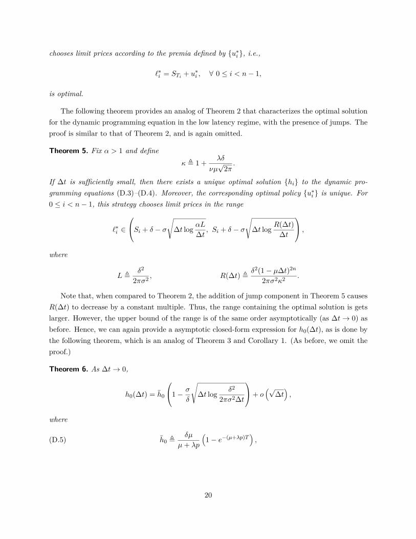
chooses limit prices according to the premia defined by {u∗i }, i.e.,
`∗i = STi + u∗i , ∀ 0 ≤ i < n− 1,
is optimal.
The following theorem provides an analog of Theorem 2 that characterizes the optimal solutionfor the dynamic programming equation in the low latency regime, with the presence of jumps. Theproof is similar to that of Theorem 2, and is again omitted.
Theorem 5. Fix α > 1 and defineκ , 1 + λδ
νµ√
2π.
If ∆t is sufficiently small, then there exists a unique optimal solution {hi} to the dynamic pro-gramming equations (D.3)–(D.4). Moreover, the corresponding optimal policy {u∗i } is unique. For0 ≤ i < n− 1, this strategy chooses limit prices in the range
`∗i ∈
Si + δ − σ
√∆t log αL∆t , Si + δ − σ
√∆t log R(∆t)
∆t
,where
L ,δ2
2πσ2 , R(∆t) , δ2(1− µ∆t)2n
2πσ2κ2 .
Note that, when compared to Theorem 2, the addition of jump component in Theorem 5 causesR(∆t) to decrease by a constant multiple. Thus, the range containing the optimal solution is getslarger. However, the upper bound of the range is of the same order asymptotically (as ∆t→ 0) asbefore. Hence, we can again provide a asymptotic closed-form expression for h0(∆t), as is done bythe following theorem, which is an analog of Theorem 3 and Corollary 1. (As before, we omit theproof.)
Theorem 6. As ∆t→ 0,
h0(∆t) = h0
1− σ
δ
√∆t log δ2
2πσ2∆t
+ o(√
∆t),
where
(D.5) h0 ,δµ
µ+ λp
(1− e−(µ+λp)T
),
20

is the zero latency limit of h0(∆t), and
p , 1− Φ(δ
ν
),
the probability of a jump size greater than δ.Furthermore, latency cost is unchanged with the introduction of the jump components in the bid
price dynamics, i.e., as ∆t→ 0,
LC(∆t) = σ√
∆tδ
√log δ2
2πσ2∆t + o(√
∆t).
Our analysis with the jump-diffusion model can be interpreted as follows. Theorem 6 illustratesthat, when there is a jump component (i.e., λ > 0), the zero latency limit h0 has a lower value thanin the absence of jumps, (i.e., λ = 0), all else being equal. In other words, the presence of jumps isdetrimental even in the absence of latency. To see why, note that jumps are zero mean innovationsin the price process. In our model, an investor only earns excess value by waiting for an impatientbuyer. Jumps may cause the bid price to cross the investor’s limit order price and execute his sharewithout giving him the chance to revise his order. Thus, jumps reduce the probability of tradingwith an impatient buyer.
This intuition can be made precise by interpreting the zero latency limit in (D.5). Observethat µ+ λp is the combined arrival rate of impatient buyers asking for an immediate execution, orpositive jumps in the price of the stock that are larger than the bid-offer spread and would resultin trade execution. The quantity
µ
µ+ λp
(1− e−(µ+λp)T
)is the probability that there at least one such arrival, and that the first such arrival is that of animpatient buyer. In this case, the trader earns a relative spread of δ. In all other cases (i.e., noarrivals, or the case where the first arrival is a large positive jump), the trade occurs at the bidprice and the trader earns no spread. These two cases yield the expression for h0.
Now, comparing with our earlier results, jumps also negatively impact the investor in thepresence of latency, for similar reasons as in the zero latency case. However, when measuredrelative to the zero latency case, i.e., in term of latency cost, jumps create no additional impact.That is, the latency cost expressions in Theorem 6 and Corollary 1 are identical. Intuitively, inour model, jumps are instantaneous, and the investor cannot react to them even in the absence oflatency. Hence, latency cost, measured relatively, only depends on the diffusive innovations.
Note that we have thus far assumed Gaussian jump sizes. In Theorem 6, the only place that thisdistribution or its parameter ν arises explicitly is the quantity p. This is the probability that thejump will be larger than the prevailing bid-offer spread, δ, and hence will cross with the limit order
21
places by the investor. This leads us to conjecture (without proof) the result in the non-Gaussiancase: if the jump size Yi in (D.1) is an i.i.d. zero mean random variable that has a cumulativedistribution function G, then Theorem 6 holds with p , 1−G(δ).
22