Embed Size (px)
Citation preview

The Cost of Decoupling Trade and Transport in the EuropeanEntry-Exit Gas Market with Linear Physics Modeling
Tom Böttger, Veronika Grimm,Thomas Kleinert, Martin Schmidt∗
Abstract. Liberalized gas markets in Europe are organized as entry-exit regimes so thatgas trade and transport are decoupled. The decoupling is achieved via the announcementof technical capacities by the transmission system operator (TSO) at all entry and exitpoints of the network. These capacities can be booked by gas suppliers and customers inlong-term contracts. Only traders who have booked capacities up-front can “nominate”quantities for injection or withdrawal of gas via a day-ahead market. To ensure feasibilityof the nominations for the physical network, the TSO must only announce technicalcapacities for which all possibly nominated quantities are transportable. In this paper,we use a four-level model of the entry-exit gas market to analyze possible welfare lossesassociated with the decoupling of gas trade and transport. In addition to the multilevelstructure, the model contains robust aspects to cover the conservative nature of theEuropean entry-exit system. We provide several reformulations to obtain a single-levelmixed-integer quadratic problem. The overall model of the considered market regimeis extremely challenging and we thus have to make the main assumption that gas �owsare modeled as potential-based linear �ows. Using the derived single-level reformulationof the problem, we show that the feasibility requirements for technical capacities implysigni�cant welfare losses due to unused network capacity. Furthermore, we �nd that thespeci�c structure of the network has a considerable in�uence on the optimal choice oftechnical capacities. Our results thus show that trade and transport are not decoupled inthe long term. As a further source of welfare losses and discrimination against individualactors, we identify the minimum prices for booking capacity at the individual nodes.
Keywords and phrases. OR in Energy, Entry-Exit Gas Market, Gas Market Design, MultilevelOptimization, Robust Optimization
1. Introduction
Starting in the 1990s, the European gas market has been liberalized step by step over thelast decades. The First and the Second Gas Directive [15, 17] paved the way for the ThirdEnergy Package [16], which was introduced in 2009. This package essentially prescribesthe decoupling of gas trade and transport via an appropriate entry-exit market designin all member states. Today, European transmission system operators (TSOs) usuallyoperate under variants of such an entry-exit regime, in which traders sign long-termcapacity contracts—so-called bookings—at entry and exit points of the network. Onlytraders who have booked capacities can afterward “nominate” quantities to feed-in (inthe case of suppliers) or withdraw (in the case of consumers) on a daily basis. Thesenominations are determined by the trade of gas (up to the individually booked capacity)on a day-ahead market. To ensure that all nominations are indeed feasible w.r.t. the givennetwork, the TSO announces so-called technical capacities up-front that limit the long-term capacity contracts (i.e., the bookings) per entry or exit point. While the entry-exitmarket design e�ectively decouples trade and transport of gas and thus might achieve tomake market interaction more transparent, it clearly comes at a cost. In particular, the
Date: April 26, 2021.2010 Mathematics Subject Classi�cation. 90-XX, 90C35, 91B15, 91B16, 91B24.∗Corresponding author: Martin Schmidt ([email protected])
1

2 T. BÖTTGER, V. GRIMM, T. KLEINERT, M. SCHMIDT
technical capacity requirement that any possible market outcome must be feasible w.r.t.the network implies that the usable network capacity signi�cantly lags behind the actualcapacity of the network. Consequently, as compared to a nodal-pricing design, it is likelythat the network capacity is not used optimally.
Our contribution addresses exactly this issue: Does the decoupling of trade and transportleave network capacity unused and ultimately results in economic ine�ciencies? To thebest of our knowledge, a detailed quantitative analysis of this e�ect is missing in theliterature up to date. The �rst paper that provides a rigorous modeling of entry-exit-likesystems is [24]. The four-level model developed in that paper comprises a two-stagemarket model that captures the booking and the nomination decisions and also includes anaccurate representation of the network. We build on this model to compare three scenarios:(i) A nodal-pricing regime, (ii) an entry-exit regime, and (iii) a hybrid model in whichtechnical capacities restrict the trade at the daily gas market, but the requirement is thatonly the market solution (instead of all possibly occurring market solutions) needs to befeasible. We interpret this model as a second-best benchmark, which would be relevant ifthe network operator could rely on experience when determining the technical capacitiesand therefore would not have to ensure that all possible nominations are feasible.
Note that the considered multilevel problems are a generalization of bilevel optimiza-tion problems that are known to be NP-hard [27, 34]. Thus, to provide an insightfulquantitative analysis we have to make several assumptions. First, the market model in [24],which we build on, is based on the assumption of perfect competition among gas traders.As a matter of fact, the consideration of strategic interaction in markets in combinationwith complex physical �ow models that restrict decisions makes an insightful analysisextremely challenging in our context. Our setup, on the contrary, allows for clear insightsinto the interplay of market interaction and physical gas transport. Furthermore, notethat even in a perfect competition setup, the interaction of economic agents on a network,which is characterized by complex physical �ow constraints, challenges standard economicanalysis. In [23], for example, it is shown that the usual equivalence between the alloca-tion in the welfare optimum and under perfect competition no longer holds. Besides thechallenges arising from the multilevel structure of the market model, a correct modelingof the technical capacities set by the TSO results in an adjustable-robustness constraint inthe upper level of the problem: The TSO must choose technical capacities such that everypossible feasible nomination is transportable. Adjustable-robust optimization problemscan be considered as two-stage optimization problems and are therefore challenging bythemselves [4, 5, 57]. From another perspective, in [39] it is shown, that the problemof validating the feasibility of a booking—and technical capacities can be interpreted asbookings—is in coNP for the case of nonlinear (but algebraic) pressure loss functionsand general networks. Going even further, a detailed modeling of gas physics introducesadditional nonlinearities up to di�erential equations to accurately model pressure lossesin pipes. Thus, and in line with the arguments in [24], we assume some reasonable simpli-�cations for the physical �ow modeling to keep the problem computationally tractable:(i) We consider only stationary gas �ow, (ii) we do not include controllable elements likecompressors or (control) valves, and (iii) we consider a potential-based gas �ow model inwhich pressure losses linearly depend on the �ow. We are aware of the fact that these phys-ical assumptions, especially the linearity of gas �ows, are strong assumptions. However,we are convinced that nonlinear gas �ow models are far out of reach due to theoreticalcomplexity reasons. We will discuss this issue later on in more detail. Nevertheless, weare convinced that our results shed some interesting light on the economic implications ofthe entry-exit gas market system in Europe.
The contribution of this paper is the following. We use the bilevel reformulationof the four-level entry-exit model presented in [24] and develop an exact single-levelreformulation. To this end, we analyze the primal-dual optimality conditions of the bilevel

THE COST OF DECOUPLING TRADE AND TRANSPORT IN THE EUROPEAN ENTRY-EXIT GAS MARKET 3
problem’s lower level in detail to derive bounds that can be used as problem-speci�c big-Ms. Moreover, we develop problem-tailored linearizations for the occurring nonsmoothand nonconvex constraints of the single-level reformulation. Finally, we re-state thechallenging robustness constraint, which is needed to specify technical capacities, as asystem of linear constraints by exploiting the characterization given in [39]. By doing so,we arrive at a model reformulation that can be tackled with state-of-the-art solvers. In acase study, we compare the results of the entry-exit regime described by this model to a�rst-best benchmark as well as a “second-best” regime in which technical capacities aredetermined as to make the resulting market allocation feasible, but not all allocations thatmight occur given the capacity restrictions at the nodes. Our case study yields severalinsights. First, we identify the cost of decoupling trade and transport by showing thatthe robustness constraint in an entry-exit market design accounts for signi�cant welfarelosses as compared to �rst-best and second-best models. Second, the design of the networkhas a signi�cant impact on the speci�cation of technical capacities at the individualnodes. Thus, our results show that, from a long-run perspective, trade and transport arenot decoupled at all. Third, the booking price �oors established by the TSO to collectpayments from the traders to reimburse transportation costs may further reduce welfareand, depending on the used pricing regime, can lead to discrimination against individualactors. Fourth, the computational e�ort required to solve the problem mostly stems fromthe robustness constraint. Finally, our second-best benchmark captures the situationin which the network operator sets the technical capacities based on experience, andtherefore, the robustness constraint does not need to be imposed in its strictest form. Asone would expect, the welfare losses are lower than under the strict robustness constraint.Less restrictive feasibility constraints might also be possible in practice if interruptiblecontracts exist for some market participants. However, this case is too complex to bemodeled and solved in the context of our formal analysis and case study.
Up to date, the literature on gas markets has mainly focused on strategic interaction ofsuppliers. Typically, stylized two-node networks are used to get insights on the potentiale�ects of market power in network based industries; see, e.g., Cremer and La�ont [12],Ikonnikova and Zwart [32], Jansen et al. [33], Meran et al. [42], Oliver et al. [46], and Yanget al. [56]. Other contributions to the gas market literature analyze strategic interactionin gas markets using complementarity problems that allow to computationally deriveequilibrium predictions. Those contributions typically rely on less restrictive assumptionsregarding the analyzed network structure. However, they do not provide general analyticalsolutions of the market interaction. Examples are Baltensperger et al. [3], Boots et al. [7],Boucher and Smeers [8, 9], Chyong and Hobbs [11], Egging et al. [13, 14], Gabriel et al. [21],Holz et al. [29], Huppmann [31], Siddiqui and Gabriel [50], and Zwart and Mulder [59].Some papers go beyond the classical linear network �ow and account for the in�uence ofpressure gradients between nodes of the network, e.g. Midthun et al. [43], Midthun et al.[44], and Rømo et al. [49]. Those papers focus on the assessment of infrastructure anddispatch for gas networks based on the so-called Weymouth equation [54]. The ine�ciencyof decoupling gas transport and trade due to unused network capacity has been argued bysome authors; see, e.g., Smeers [51]. By now, however, a detailed analysis is missing. Still,there are some illustrative examples, e.g., in, Alonso et al. [1], Glachant et al. [22], Hallackand Vazquez [26], Hirschhausen [28], Hunt [30], and Vazquez et al. [52].
The paper is structured as follows. In Section 2, we review each level of the four-levelmodel from [24] in detail and also state the bilevel reformulation given in [24]. Then, wedevelop an equivalent single-level reformulation of the model in Section 3 and proposefurther reformulations in Section 4. In Section 5, we tackle the robustness constraint.Finally, in Section 6 we measure ine�ciencies arising in entry-exit-like systems andconclude in Section 7.

4 T. BÖTTGER, V. GRIMM, T. KLEINERT, M. SCHMIDT
2. A Multilevel Model of the Entry-Exit Gas Market
In this section, we review the four-level model of the European entry-exit gas marketas it has been developed in [24]. We briefly introduce each level and state an equivalentbilevel reformulation of the four-level model. All other details and the rationale of themultilevel modeling are given in [24].
In a nutshell, the four levels of the considered market environment model the followingsequence of actions:
(i) Speci�cation of technical capacities and booking price �oors by the TSO.(ii) Booking of capacity rights by gas buying and selling �rms.
(iii) Day-ahead nomination by gas buying and selling �rms.(iv) Cost-optimal transport of the realized nominations by the TSO.
Before we formally state the particular optimization problem of each level we introducesome notation. Gas transport networks are modeled as a directed graph G = (V ,A) withnode set V and arc set A. The node set is split up into the set of entry nodes V+ ⊆ V atwhich gas is supplied, the set of exit nodes V− ⊆ V at which gas is discharged, and the setof inner nodes V0 ⊆ V without gas supply or withdrawal. Thus, V = V+ ∪V− ∪V0. Themodel allows for multiple gas selling or gas buying �rms i ∈ Pu for u ∈ V+ or u ∈ V−,respectively.
Due to the general hardness of the four-level model, we need some important sim-plifying assumptions. In particular, we do not consider controllable elements such ascompressors or control valves, we consider stationary gas �ow, and we assume a linearpressure loss function. We will discuss these assumptions in more detail later, when theyare formally introduced. We now describe every level in detail.
2.1. Level 1: Speci�cation of Technical Capacities and Booking Price Floors. Inthe �rst of the four levels of the model, the TSO speci�es technical capacities and price�oors in order to maximize total social welfare obtained in the market:
maxqTC,
¯π book
∑t ∈T
( ∑u ∈V−
∑i ∈Pu
∫ qnomi ,t
0Pi ,t (s) ds −
∑u ∈V+
∑i ∈Pu
cvari qnom
i ,t
)− φ4(qnom) −C (1a)
s.t. 0 ≤ qTCu , 0 ≤
¯π booku for all u ∈ V+ ∪V−, (1b)∑
u ∈V+∪V−
∑i ∈Pu
¯π booku qbook
i = φ4(qnom) +C, (1c)
∀q̂nom ∈ N(qTC) : F (q̂nom) , ∅, (1d)
qbooki ∈ arg max (3) for all i ∈ Pu , u ∈ V+ ∪V−, (1e)
qnomi ,t ∈ arg max (4) for all i ∈ Pu , u ∈ V+ ∪V−, t ∈ T . (1f)
Since we consider multiple time periods of gas trading and transport, total social welfareis aggregated over all time periods t ∈ T with |T | < ∞. Gas buying �rms are modeled bystrictly decreasing inverse market demand functions Pi ,t , i ∈ Pu , u ∈ V−, and gas selling�rms are characterized by pairwise distinct variable costs of production cvar
i , i ∈ Pu ,u ∈ V+.Throughout the paper, φk denotes the optimal value of the kth level of the multilevelmodel, i.e., k ∈ {1, 2, 3, 4}. For instance, φ4 denotes the minimum costs of gas transportobtained in the fourth level. The decision variables of the �rst level include the technicalcapacities qTC
u for every entry and exit node u ∈ V+ ∪V− of the network. These variableslimit the booking quantities qbook
i of the players i , which are decided on the second level;see Constraint (1e). The second set of �rst-level decision variables consists of the price�oors
¯π booku for booking quantities at every entry and exit nodeu ∈ V+∪V−. Constraint (1c)
models that the booking price �oors are chosen such that the transport costs φ4(qnom)
arising in level four plus additional exogenously given network costs C , e.g., investment

THE COST OF DECOUPLING TRADE AND TRANSPORT IN THE EUROPEAN ENTRY-EXIT GAS MARKET 5
costs, are recovered. The actual nominations qnomi ,t are decided on the third level; see (1f).
Note that exactly these nominations are entering the objective function of the �rst level.Finally, we consider the Constraint (1d). This constraint claims that in dependence of
the technical capacities qTC all balanced nominations that potentially may occur, i.e.,
N(qTC) :=
{q ∈ RV+∪V− : 0 ≤ q ≤ qTC,
∑u ∈V+
qu =∑u ∈V−
qu
},
need to be feasible with respect to the network. In other words: Every balanced andnode-wise aggregated nomination that satis�es given technical capacities needs to betransportable. This is formalized by the condition F (q̂nom) , ∅, where F (q̂nom) is theset of feasible points of the cost-minimization transport problem in the fourth level. Wediscuss this feasible set in more detail in Section 2.4. Constraint (1d) corresponds to an∃-∀-∃ quanti�er structure, i.e., there must exist a vector of technical capacities qTC suchthat for all possible nominations q̂nom ∈ N(qTC) there exists a feasible point in F (q̂nom).Thus, from the viewpoint of robust optimization (cf., e.g., [4, 6] and the many referencestherein), the constraint can be interpreted as an adjustable-robust and thus semi-in�niteconstraint [57] with here-and-now decisions qTC and wait-and-see decisions in the feasibleset of the fourth level. As such, Constraint (1d) adds signi�cant di�culty to the overallmodel. We will discuss the handling of this constraint in more detail in Section 5 and itscomputational implications in Section 6.2. As previously mentioned, Constraint (1d) isalso problematic from an economic point of view. Since every balanced nomination thatis feasible w.r.t. the technical capacities must be guaranteed to be transportable by theTSO, this constraint is suspect to leave network capacities unused. Thus, it is very likelythat the robustness constraint causes ine�ciencies. The analysis of this e�ect is the mainmotivation for this paper and is taken care of in Section 6. Let us mention at this pointthat we are aware of that, in practice, the TSO might not respect the Constraint (1d) inits strictest form. Instead, she might draw on experience and set technical capacities thatguarantee feasibility for likely market outcomes but not for all possible nominations. Weaccount for this by analyzing a respective scenario in the case study in Section 6. Moreover,there are further capacity products such as so-called conditional, restrictively allocable, orinterruptible capacities that are used to give the TSO more �exibility to ensure feasibilityof the actually realized loads. The modeling of these capacity products is out of scope ofthis paper and we refer to Chapter 3 in the book [38] for additional details.
2.2. Level 2: Booking. At this level, each player i ∈ Pu with u ∈ V− ∪V+ books capacityrights qbook
i to maximize the anticipated revenue φ3i ,t (realized in the third level; see
Section 2.3) minus booking costs. In line with [24], we assume perfect competition. Inparticular, we assume that bookings are not made strategically. This disallows to excludecompetitors from the market by preemptive bookings and to drive up spot-market prices.The model of each player then reads as follows:
maxqbooki
∑t ∈T
φ3i ,t (q
booki ) − (
¯π booku + π book
u )qbooki
s.t. qbooki ≥ 0,∑i ∈Pu
qbooki ≤ qTC
u .
(2)
Players potentially compete for scarce technical capacities qTC that are outcome of the �rstlevel. The booking price �oor
¯π booku , that is also outcome of the �rst level, always applies
for every booking. The additional markup π booku only occurs in case of scarce technical
capacities, i.e., as the result of a competitive bidding process for the bookings. It is shownin [24] that the Problems (2) can be aggregated node-wise to obtain a mixed nonlinearcomplementarity problem (MNCP) per node under some additional assumptions. In the

6 T. BÖTTGER, V. GRIMM, T. KLEINERT, M. SCHMIDT
case study in Section 6, we only consider a single player i per node u. We thus refrainfrom a discussion of these assumptions here. The reasoning behind the modeling decisionof one player per node is given in Section 6. In Theorem 1 in [24] it is further shown thatthe above mentioned MNCP is equivalent to the optimization problem
φ2u (q
TCu , ¯
πu ) := maxqbooki
∑i ∈Pu
∑t ∈T
φ3i ,t (q
booki ) −
¯π booku qbook
i (3a)
s.t. qbooki ≥ 0 for all i ∈ Pu , (3b)∑i ∈Pu
qbooki ≤ qTC
u , (3c)
in which the markup price π booku is exactly the dual variable of Constraint (3c). This
problem is solved at every entry and exit node of the network and all these problems areindependent of each other.
2.3. Level 3: Nomination. At the third level, all players choose nominations restrictedby their bookings of the second level in order to maximize their individual surplus atthe equilibrium market price πnom
t , which results endogenously at the third level. Underperfect competition, all players act as price takers. Thus, every gas seller i ∈ Pu , u ∈ V+,maximizes its surplus in every time period t ∈ T :
φ3i ,t (q
booki ) := max
qnomi ,t
(πnomt − cvar
i )qnomi ,t s.t. 0 ≤ qnom
i ,t ≤ qbooki .
Similarly, every gas buyer i ∈ Pu , u ∈ V−, maximizes its bene�t in every time period t ∈ T :
φ3i ,t (q
booki ) := max
qnomi ,t
∫ qnomi
0Pi ,t (s) ds − πnom
t qnomi ,t s.t. 0 ≤ qnom
i ,t ≤ qbooki .
Using �rst-order optimality conditions for every maximization problem, the nominationlevel can be modeled as an MNCP; see [24]. In Theorem 3 in [24] it is further shown thatthe resulting MNCP can be recast as an equivalent welfare maximization problem:
φ3(qbook) := maxqnom
∑t ∈T
( ∑u ∈V−
∑i ∈Pu
∫ qnomi ,t
0Pi ,t (s) ds −
∑u ∈V+
∑i ∈Pu
cvari qnom
i ,t
)(4a)
s.t. 0 ≤ qnomi ,t ≤ qbook
i for all i ∈ Pu , u ∈ V+ ∪V−, t ∈ T , (4b)∑u ∈V−
∑i ∈Pu
qnomi ,t −
∑u ∈V+
∑i ∈Pu
qnomi ,t = 0 for all t ∈ T . (4c)
Constraint (4c) is the market clearing condition. The dual variable of this constraint is themarket price πnom
t in time period t ∈ T .
2.4. Level 4: Cost-Optimal Transport of Nominations. The fourth level is concernedwith the cost-optimal transport of the nominations that are the outcome of the third level.The TSO solves the minimization problem
minp,q
∑t ∈T
ct (qnom) s.t. (p,q) ∈ F (qnom),
where ct (qnom) is the transportation cost for the given nomination qnom.For the speci�cation of the feasible set F (qnom) that restricts gas pressures p and gas
mass �ows q, we follow [25] and [39]. For every node u ∈ V of the gas transport networkand time period t ∈ T we denote the gas pressure by pu ,t with bounds
0 < p−u ≤ pu ,t ≤ p+u ≤ ∞.
Further, gas mass �ow on arc a ∈ A in time period t is denoted by qa,t . For an arc a = (u,v),qa,t > 0 is interpreted as �ow in the direction of the arc, i.e., from u to v , and qa,t < 0

THE COST OF DECOUPLING TRADE AND TRANSPORT IN THE EUROPEAN ENTRY-EXIT GAS MARKET 7
as �ow in the opposite direction. Additionally, the gas mass �ow has to satisfy givencapacities
−∞ ≤ q−a ≤ qa,t ≤ q+a ≤ ∞ for all a ∈ A, t ∈ T , (5)and mass balance at every node of the network is modeled using the constraints∑
a∈δ outu
qa,t −∑a∈δ in
u
qa,t =∑i ∈Pu
qnomi ,t for all u ∈ V+, t ∈ T ,∑
a∈δ outu
qa,t −∑a∈δ in
u
qa,t = −∑i ∈Pu
qnomi ,t for all u ∈ V−, t ∈ T ,∑
a∈δ outu
qa,t −∑a∈δ in
u
qa,t = 0 for all u ∈ V0, t ∈ T .
(6)
In this formulation, δoutu represents outgoing edges and δ in
u represents incoming edges atnode u.
Further, gas pressure needs to be coupled at the incident nodes of an arc with the arc’sgas mass �ow. In a rather general form, this is achieved by the pressure loss law
p2u ,t − p
2v ,t = Φa(qa,t ) for all a = (u,v) ∈ A, t ∈ T ,
where Φa denotes the pressure loss function for arc a ∈ A. We can substitute the squaredpressure variables using πu ,t = p2
u ,t for all u ∈ V , t ∈ T , and obtain the constraintsπu ,t − πv ,t = Φa(qa,t ) for all a = (u,v) ∈ A, t ∈ T , (7)
together with the bounds0 < π−u ≤ πu ,t ≤ π
+u ≤ ∞ for all u ∈ V , t ∈ T . (8)
We make the following assumption.
Assumption 1. The pressure loss function Φa is linear for all a ∈ A.
This assumption renders the transport model of this section linear. Technically, thisassumption is not needed for the bilevel reformulation in Section 2.5 and the single-level reformulation in Section 3. However, without this assumption, the transport modeloccurring in the upper level of the bilevel problem will be nonlinear, which furthercomplicates an already challenging problem. Moreover, the linear reformulation of therobustness constraint (1d) stated in Section 5 is not possible without Assumption 1 unlesscompact global optimality certi�cates are available for nonconvex problems. This, however,is strongly related to the P vs. NP problem, which is why Assumption 1 is needed forreasons of computational tractability.
Lastly, we need to specify the transportation costs. As mentioned, we only considerpassive gas transport networks in this paper. These are networks that do not containcontrollable network elements like compressors or (control) valves. However, transporta-tion costs mainly arise from these controllable elements such as compressors. Usually,transportation costs are driven by pressure losses across the network. In order to mimiccost-optimal transport in our setting, the objective function in the fourth level minimizescosts of squared pressure losses in the entire network that are given by the nonsmoothexpression ∑
t ∈T
∑a=(u ,v)∈A
c transt |πu ,t − πv ,t |,
where c transt > 0 is a parameter. In total, the problem at level four reads
φ4(qnom) := minπ ,q
∑t ∈T
∑a=(u ,v)∈A
c transt |πu ,t − πv ,t | s.t. (5)–(8). (9)

8 T. BÖTTGER, V. GRIMM, T. KLEINERT, M. SCHMIDT
TSO Market1: TechnicalCapacity 2: Booking
3: Nomination4: Cost-Optimal
Transport
qTC,¯π book
qbook
qbookφ3
qnom
qnomφ4
Figure 1. Dependencies between the four levels; taken from [24].
2.5. Reduction to a Bilevel Problem. The structure of the four-level model presented inthe previous sections is rather complicated. Figure 1 sheds more light on the dependenciesof the levels and the structure of the full model. It can be seen that, e.g., the variables ofthe fourth level do not appear in the constraints of any other level. In Section 3 of [24] itis shown that this structure can be exploited to equivalently re-state the four-level modelas a bilevel model. In particular, in Theorem 5 in [24] it is shown that the original second-and third-level problem can be merged into an equivalent single-level problem. Thus, thefour-level model can be reduced to an equivalent trilevel one. In addition, in Theorem 7in [24] it is shown that this trilevel model can be further reduced to the following bilevelmodel by merging the original fourth-level problem into the original �rst-level problem.
maxqTC,
¯π book,π ,q
φu(qnom, π ) =∑t ∈T
( ∑u ∈V−
∑i ∈Pu
∫ qnomi ,t
0Pi ,t (s) ds −
∑u ∈V+
∑i ∈Pu
cvari qnom
i ,t
)−
∑t ∈T
∑a=(u ,v)∈A
c transt (|πu ,t − πv ,t |) −C
(10a)
s.t. 0 ≤ qTCu , 0 ≤
¯π booku for all u ∈ V+ ∪V−, (10b)∑
u ∈V+∪V−
∑i ∈Pu
¯π booku qbook
i =∑t ∈T
∑a=(u ,v)∈A
c transt |πu ,t − πv ,t | +C, (10c)
∀q̂nom ∈ N(qTC) : F (q̂nom) , ∅, (10d)(π ,q) ∈ F (qnom), i.e., π ,q ful�ll (5)–(8) (10e)
(qbook,qnom) ∈ arg max (11), (10f)

THE COST OF DECOUPLING TRADE AND TRANSPORT IN THE EUROPEAN ENTRY-EXIT GAS MARKET 9
1 & 4: Technical Capacity &Cost-Optimal Transport
2 & 3: Booking & Nomination
qTC,¯π bookqbook, qnom
Figure 2. Dependencies between the two levels of the reduced bilevelproblem; taken from [24].
where the lower level is given by
maxqbook,qnom
∑t ∈T
( ∑u ∈V−
∑i ∈Pu
∫ qnomi ,t
0Pi ,t (s) ds −
∑u ∈V+
∑i ∈Pu
cvari qnom
i ,t
)(11a)
−∑
u ∈V+∪V−
∑i ∈Pu
¯π booku qbook
i
s.t.∑i ∈Pu
qbooki ≤ qTC
u for all u ∈ V+ ∪V−, [π booku ] (11b)
0 ≤ qnomi ,t ≤ qbook
i for all i ∈ Pu , u ∈ V+ ∪V−, t ∈ T , [γ±i ,t ] (11c)∑u ∈V−
∑i ∈Pu
qnomi ,t −
∑u ∈V+
∑i ∈Pu
qnomi ,t = 0 for all t ∈ T . [πnom
t ] (11d)
The upper level (10) represents the combined �rst and fourth level of the original four-levelmodel, i.e., the TSO’s actions, whereas the lower level (11) consists of the original secondand third level and models the market interaction. The lower-level problem has a uniquesolution under reasonable assumption, see Theorem 6 in [24], so that we do not haveto consider aspects related to optimistic or pessimistic bilevel solutions. Note that weomitted the redundant second-level constraint 0 ≤ qbook
i since it is trivially ful�lled dueto Constraint (11c). The dependencies between the two levels are illustrated in Figure 2.The bilevel structure is one of the major challenges of the problem. Bilevel problemsare inherently nonconvex and even linear bilevel problems are NP hard [27, 34]. Apartfrom that the problem is challenging because the upper level itself is challenging dueto at least three reasons. First, the upper level has nonsmooth terms in the objectivefunction and in Constraint (10c). Second, Constraint (10c) contains nonconvex bilinearterms
¯π booku qbook
i . Third, and most importantly, the upper level contains the semi-in�niterobustness constraint (10d), which is, in general, not tractable from a computational pointof view. We tackle the bilevel structure in Section 3, the nonsmooth and bilinear termsof the upper level in Section 4, and the robustness constraint in Section 5. Finally, wepoint out that without Assumption 1, the modeling of the gas transport in Constraint (10e)would be nonlinear and thus introduce additional di�culties to the upper level of thebilevel reformulation.
2.6. BenchmarkModels. Due to the overall hardness of Problem (10), we introduce tworelaxations that serve as a benchmark in the following.
A �rst-best benchmark can be obtained by optimizing the total welfare considering boththe network and market interaction constraints. In bilevel programming, this corresponds

10 T. BÖTTGER, V. GRIMM, T. KLEINERT, M. SCHMIDT
to the so-called high-point relaxation; see [45]. From an economic perspective this �rst-best benchmark assumes an integrated gas company that is fully regulated and that takesall decisions in a welfare-optimal manner. Consequently, we can remove the need for aprior determination of technical capacities and bookings. This renders also the robustnessconstraint (10d) redundant. We thus obtain a model that determines the decisions of theoriginal third and fourth level, accounting for welfare optimal production and demand aswell as cost-optimal transport simultaneously:
maxqnom≥0,π ,q
φu(qnom, π ) s.t. (qnom, π ,q) satis�es (5)–(8). (12)
Another benchmark model can be obtained by omitting only the robustness con-straint (10d), which is one of the major di�culties of the bilevel problem (10):
maxqTC,
¯π book,π ,q
φu(qnom, π ) (13a)
s.t. (10b), (10c), and (10e), (13b)
(qbook,qnom) ∈ arg max (11). (13c)From an economic point of view this model assumes that the TSO needs to make sure thatonly realized nominations need to be transportable. Thus, this model serves as a directbenchmark to measure the ine�ciencies caused by the robustness constraint (10d). In thissense, Problem (13) can be interpreted as a second-best model that captures, for instance,a situation in which the network operator is able to set the technical capacities based onexperience.
It is easy to see that out of the three models, Problem (12) yields the best welfareoutcome and bounds the welfare outcome of Problem (13). The latter, in turn, obviouslybounds the welfare outcome of the bilevel reformulation (10) of the four level entry-exitmodel. In Section 6, we use this model hierarchy to measure ine�ciencies in entry-exit-likesystems.
3. Reduction to a Single-Level Problem
In the previous section we discussed a four-level model of an entry-exit-like system andreduced it to an equivalent bilevel problem with a convex lower level as described in [24]. Inrecent years, several algorithms evolved for bilevel problems that exploit certain structuralproperties. However, most—if not all—bilevel-tailored algorithms whose performancecould be demonstrated in computational studies, e.g., [18, 35, 40, 55], are either onlyapplicable to (mixed-integer) linear bilevel problems or rely on the property of integerlinking variables (upper-level variables that are present in the lower-level constraints).All these algorithms are not appropriate for our setting of nonlinear upper- and lower-level problems and continuous linking variables qTC and
¯π book. Thus, we resort to the
well-known standard technique of replacing the convex lower level by its necessary andsu�cient �rst-order optimality conditions to obtain a single-level problem. Note thatthis approach requires Slater’s constraint quali�cation to hold. In the following, we �rstperform a single-level reformulation based on the Karush–Kuhn–Tucker (KKT) conditionsand, in a second step, we provide an exact mixed-integer linear reformulation of the KKTcomplementarity conditions.
3.1. A KKT-Based Single-Level Reformulation. A single-level reformulation can beobtained by replacing (10f) either by the strong duality conditions or the KKT conditionsof Problem (11). In any way, we use the following assumption to obtain a computationallytractable reformulation.
Assumption 2. All inverse market demand functions are linear and strictly decreasing, i.e.,Pi ,t (q
nomi ,t ) = ai ,t + bi ,tq
nomi ,t with ai ,t > 0 and bi ,t < 0.

THE COST OF DECOUPLING TRADE AND TRANSPORT IN THE EUROPEAN ENTRY-EXIT GAS MARKET 11
This yields concave-quadratic upper- and lower-level objective functions w.r.t. theupper- or lower-level variables, respectively. Thus, with Assumption 2, the lower-levelproblem (11) is a concave-quadratic maximization problem over linear constraints andthe strong-duality theorem of convex optimization is applicable. Furthermore, its KKTconditions are both necessary and su�cient; see, e.g., [10]. Following the strong-dualityapproach, one would replace the lower level by primal and dual feasibility as well as thestrong-duality equation. Even for linear objective functions, the strong-duality equationof the lower level yields nonconvex bilinear terms of primal upper-level variables anddual lower-level variables; see, e.g., [58]. Thus, we refrain from using the strong-dualityreformulation and instead replace the lower-level problem by its KKT conditions, i.e., bythe stationarity conditions
−¯π booku − π book
u +∑t ∈T
γ+i ,t = 0 for all i ∈ Pu , u ∈ V+ ∪V−, (14a)
ai ,t + bi ,tqnomi ,t + γ
−i ,t − γ
+i ,t − π
nomt = 0 for all i ∈ Pu , u ∈ V−, t ∈ T , (14b)
−cvari + γ
−i ,t − γ
+i ,t + π
nomt = 0 for all i ∈ Pu , u ∈ V+, t ∈ T , (14c)
primal feasibility (11b)–(11d), nonnegativity
π booku ≥ 0 for all u ∈ V+ ∪V−, (15a)
γ−i ,t ,γ+i ,t ≥ 0 for all i ∈ Pu , u ∈ V+ ∪V−, t ∈ T , (15b)
and complementarity constraints
π booku
(qTCu −
∑i ∈Pu
qbooki
)= 0 for all u ∈ V+ ∪V−, (16a)
γ−i ,tqnomi ,t = 0 for all i ∈ Pu , u ∈ V+ ∪V−, t ∈ T , (16b)
γ+i ,t
(qbooki − qnom
i ,t
)= 0 for all i ∈ Pu , u ∈ V+ ∪V− t ∈ T . (16c)
Then, the bilevel problem (10) can be equivalently rephrased as the single-level problemmaxz
φu(qnom, π )
s.t. upper-level feasibility: (10b)–(10e),lower-level KKT conditions: (11b)–(11d), (14)–(16),
(17)
where z = (qTC,¯π book,qbook,qnom, π ,q, πnom, π book,γ±) is the vector of primal upper-level
as well as primal and dual lower-level variables.
3.2. Linearization of KKTComplementarity Conditions. The complementarity con-ditions (16) are nonconvex but can be linearized using additional binary variables andbig-M constants; see [19]. For a linear constraint a>x ≤ b and its dual variable λ ≥ 0, thecomplementarity condition reads
λ(b − a>x) = 0. (18)For suitable primal and dual big-M constants Mp , Md and a binary variable u ∈ {0, 1}, (18)can be linearized as follows:
b − a>x ≤ Mpu, λ ≤ Md (1 − u). (19)Finding suitable values for Mp and Md is crucial for a correct linearization. Often, thesevalues are obtained heuristically. In a bilevel context, this may result in suboptimal orinfeasible solutions [47]. In fact, �nding correct big-Ms may in general be as hard as solvingthe original bilevel problem [36]. Sometimes, however, problem-speci�c knowledge can beused to obtain correct big-M values. In our application, �nding primal big-Ms Mp is easybecause qTC, qbook, and qnom are bounded by, e.g., the maximum demand of all gas buyers.Finding dual big-Ms Md is more complicated. In the following, we derive suitable values

12 T. BÖTTGER, V. GRIMM, T. KLEINERT, M. SCHMIDT
similar to [37]. Therefore, we use the notation P− := ∪u ∈V−Pu and P+ := ∪u ∈V+Pu as wellas amin
t := min{ai ,t : i ∈ P−}, amaxt := max{ai ,t : i ∈ P−}, cvar
min := min{cvari : i ∈ P+}, and
cvarmax := max{cvar
i : i ∈ P+} and make the following assumption.
Assumption 3. For every t ∈ T it holds amint ≥ cvar
min and amaxt ≥ cvar
max .
The economic rationale is that every player is eager to participate in the market inevery time period t . The gas buyer with the smallest initial willingness to pay amin
t couldpotentially buy gas from the seller with the lowest variable costs cvar
min and the seller withthe highest variable costs cvar
max could potentially sell gas to the buyer with the highest initialwillingness to pay amax
t . This assumption can be easily checked a priori. Furthermore, weassume that the network is designed in a way such that in every time period we havetrade.
Assumption 4. For every time period t ∈ T there exists a player i ∈ V+ ∪V− with qnomi ,t > 0.
We �rst derive bounds on the free dual variable πnomt . As described in Section 2.3,
this variable corresponds to the market price for gas in time period t ∈ T . We do notneed bounds on this variable for a correct linearization of the KKT complementarityconditions (16), but bounds on πnom
t will help to bound the other dual variables.
Lemma 1. For every t ∈ T , it holds cvarmin ≤ π
nomt ≤ amax
t .
Proof. Due to Assumption 4 and the market clearing condition (11d), there must existplayers i− ∈ P− and i+ ∈ P+ with qnom
i−,t > 0 and qnomi+,t > 0. Applying KKT complementar-
ity (16b) and dual feasibility (14b) to i− and i+, one obtainsπnomt = ai−,t + bi−,tq
nomi−,t − γ
+i−,t < ai−,t ≤ amax
t and πnomt = cvar
i+ + γ+i+,t ≥ cvar
i+ ≥ cvarmin,
respectively. �
We now turn to the dual variables γ±i ,t . The variable γ−i ,t denotes the price range thatthe market price πnom
t would have to decrease (for gas buyers) or increase (for gas sellers)for player i to enter the market in time period t . Contrary, γ+i ,t indicates the bene�t ofplayer i when trading a further unit.
Lemma 2. It exists an optimal solution of the single-level reformulation (17) withγ−i ,t ≤ 2
(amaxt − cvar
min)
and γ+i ,t ≤ amaxt − cvar
min
for all time periods t ∈ T and i ∈ P+ ∪ P−.
Proof. We only consider exit nodes u ∈ V−. The case of u ∈ V+ can be shown in exactlythe same way. Let t ∈ T and let z be an optimal solution for (17) with qbook
u , qnomu ,t ,
¯π booku ,
πnomt , π book
u , and γ±u ,t being part of this optimal solution. We distinguish two cases:(i)
∑i ∈Pu q
booki > 0 and
(ii)∑
i ∈Pu qbooki = 0.
In case of (i), there exists a player i− ∈ Pu with qbooki− > 0. If qnom
i−,t > 0, KKT complemen-tarity (16b) yields γ−i−,t = 0 and the stationarity condition (14b) simpli�es to
γ+i−,t = ai−,t − πnomt + bi−q
nomi−,t < ai−,t − π
nomt ≤ amax
t − cvarmin
by applying bi− < 0 and Lemma 1. If on the other hand qnomi−,t = 0, KKT complementar-
ity (16c) yields γ+i−,t = 0 and from KKT stationarity (14b) we obtain
γ−i−,t = πnomt − ai−,t ≤ amax
t − cvarmin
by using Lemma 1 and Assumption 3. Thus, the claim is ful�lled in Case (i).We now turn to Case (ii). In this case, qbook
i = qnomi = 0 holds. Let i ∈ Pu . We set
˜¯π booku :=
∑t ∈T
(amaxt − cvar
min)
and π̃ booku := 0

THE COST OF DECOUPLING TRADE AND TRANSPORT IN THE EUROPEAN ENTRY-EXIT GAS MARKET 13
as well asγ̃−i ,t := amax
t − ai ,t + πnomt − cvar
min and γ̃+i ,t := amaxt − cvar
min. (20)Now, let z̃ be the vector that we obtain by replacing the corresponding entries of z by˜¯π booku , π̃ book
u , and γ̃±u ,t . It is easy to see that stationarity (14a) and (14b) as well as comple-mentarity (16) is ful�lled. Further, nonnegativity (10b) of ˜
¯π booku and nonnegativity (15b)
of γ̃±i ,t hold due to Lemma 1 and Assumption 3. Primal feasibility (11b)–(11d) of thelower level remains unchanged and the upper-level constraint (10c) still holds because∑
i ∈Pu ¯π booku qbook
i =∑
i ∈Pu ˜¯π booku qbook
i = 0 according to qbooki = 0. All other upper-level
constraints are trivially ful�lled by the modi�ed vector z̃, and z̃ is thus feasible for (17).Since the objective function value is not a�ected by the modi�cations, z̃ is also optimal.Finally, from (20) we obtain
γ̃−i ,t ≤ amaxt − cvar
min + amaxt − cvar
min = 2(amaxt − cvar
min)
due to Lemma 1 and Assumption 3 andγ̃+i ,t = amax
t − cvarmin.
Thus, also in Case (ii) the claim is ful�lled. �
The dual variable π booku denotes the markup price for bookings; see the discussion in
Section 2.2. It can be bounded as follows.
Lemma 3. It exists an optimal solution of the single-level reformulation (17) with
π booku ≤
∑t ∈T
(amaxt − cvar
min)
for all u ∈ V+ ∪V−.
Proof. From KKT stationarity (14a), the nonnegativity of¯π booku (see Constraint (10b)), and
Lemma 2, we obtain
π booku =
∑t ∈T
γ+i ,t − ¯π booku ≤
∑t ∈T
(amaxt − cvar
min). �
In total, we can now replace Constraint (16) in the single-level reformulation (17) by itslinearized variant according to (19). Finally, we end up with a single-level problem that issigni�cantly larger than the bilevel problem (10) due to additional continuous and binaryvariables and constraints. As previously mentioned, this single-level problem still containsnonsmooth and nonconvex terms in the objective function and in Constraint (10c) andthe semi-in�nite robustness constraint (10d). In the following Sections 4 and 5 we furtherreformulate the single-level problem to obtain a computationally tractable problem.
4. Further Reformulations of the Upper Level
In this section, we linearize the nonsmooth absolute values |πu ,t−πv ,t | and deal with thenonconvex bilinear terms
¯π booku qbook
i that both appear in the single-level reformulation (17).First, we take care of the former. Without Constraint (10c), the absolute values would onlyappear in the objective function (10a). In this case, they could be linearized with standardtechniques by introducing additional continuous variables and constraints. However,Constraint (10c) couples the absolute values |πu ,t − πv ,t | to the bilinear terms
¯π booku qbook
i .Thus, besides additional continuous variables ∆πu ,v ,t ≥ 0 for all a = (u,v) ∈ A, t ∈ T , wealso need additional binary variables xa,t for all a ∈ A, t ∈ T and the constraints
∆πu ,v ,t ≥ πu ,t − πv ,t , ∆πu ,v ,t ≤ 2π+v xa,t + πu ,t − πv ,t , (21a)∆πu ,v ,t ≥ πv ,t − πu ,t , ∆πu ,v ,t ≤ 2π+u (1 − xa,t ) + πv ,t − πu ,t , (21b)
for all a = (u,v) ∈ A, t ∈ T . It is easy to see that for xa,t = 0, Constraints (21a) areactive and enforce ∆πu ,v ,t = πu ,t − πv ,t , whereas Constraints (21b) are inactive due to the
14 T. BÖTTGER, V. GRIMM, T. KLEINERT, M. SCHMIDT
squared pressure bounds (8). The same holds with �ipped roles for xa,t = 1. We can thusreplace all terms |πu ,t − πv ,t | by the continuous variables ∆πu ,v ,t and Constraints (21).
Second, we turn to the bilinear terms in Constraint (10c). Given upper bounds ¯¯π booku
for¯π booku and q̄book
i for qbooki for every u ∈ V+ ∪V− and i ∈ Pu , these bilinear terms can be
approximated using a piecewise linearization such as, e.g., the incremental method. See[53] for a detailed overview and a numerical comparison of existing methods. On the otherhand, modern solvers like, e.g., Gurobi, can handle bilinear terms by using McCormickenvelopes [41] in combination with spatial branching. A preliminary numerical studyrevealed that in our case the latter approach using Gurobi 9 works signi�cantly better interms of running times. Since the spatial-branching-based approach also requires upperbounds for both continuous variables
¯π booku and qbook
i , we derive them in the following.We �rst state bounds for
¯π booku .
Lemma 4. It exists an optimal solution of the single-level reformulation (17) with
¯π booku ≤
∑t ∈T
(amaxt − cvar
min)
for all u ∈ V+ ∪V−.
Proof. From the lower-level KKT stationarity condition (14a), nonnegativity (15a), andLemma 2, we obtain
¯π booku =
∑t ∈T
γ+i ,t − πbooku ≤
∑t ∈T
(amaxt − cvar
min). �
In order to bound qbooki , we �rst discuss that it is feasible to express bookings in terms
of maximal nominations, i.e., to set q̄booki = maxt ∈T {qnom
i }.
Lemma 5. Suppose a player i ∈ Pu at a node u ∈ V+ ∪V− with
maxt ∈T{qnom
i ,t } < qbooki .
Then, it holds¯π booku = π book
u = 0.
Proof. Let i ∈ Pu be a player at node u ∈ V+ ∪V− with maxt ∈T {qnomi ,t } < qbook
i . Then, weknow from KKT complementarity (16c) that the dual variables γ+i ,t must be zero for allt ∈ T . Thus, KKT stationarity (14a) and nonnegativity (15a) and (10b) give
0 ≤ π booku = −
¯π booku ≤ 0,
i.e.,¯π booku = π book
u = 0. �
This means that player i ∈ Pu ,u ∈ V+∪V−, only books above the maximum nomination,if the booking price �oor
¯π booku and the markup π book
u are zero. In other words, theremaining booking ∆book
i = qbooki −maxt ∈T {qnom
i ,t } > 0 does not a�ect the total welfare φ1,which yields the following corollary.
Corollary 1. Among the optimal solutions of the bilevel problem (10), there exists a solutionfor which
maxt ∈T{qnom
i ,t } = qbooki
holds for all i ∈ P, u ∈ V+ ∪V−.
Thus, we can bound bookings by bounds for nominations. Since nominations must befeasible for the physical network, we can bound nominations by the capacity of adjacentarcs a to the node u.
THE COST OF DECOUPLING TRADE AND TRANSPORT IN THE EUROPEAN ENTRY-EXIT GAS MARKET 15
Proposition 1. With
q̄nomi =
∑a=(u ,v)∈A
max{0,q+a } +∑
a=(v ,u)∈A
max{0,−q−a } for all i ∈ Pu ,u ∈ V+,
q̄nomi =
∑a=(u ,v)∈A
max{0,−q−a } +∑
a=(v ,u)∈A
max{0,q+a } for all i ∈ Pu ,u ∈ V−,
it holds0 ≤ qnom
i ,t ≤ q̄nomi
for all i ∈ Pu , u ∈ V+ ∪V− and t ∈ T .
Since the bounds q̄nomi are independent of t ∈ T , we directly obtain the following
corollary from Corollary 1 and Lemma 1.
Corollary 2. It holds 0 ≤ qbooki ≤ q̄nom
i = q̄booki for all i ∈ Pu , u ∈ V+ ∪V−.
The derived bounds can now be used in a spatial branching approach to tackle thebilinear terms
¯π booku qbook
i .
5. Handling of the Upper Level’s Robustness Constraint
In this section, we deal with the robustness constraint (10d) that is part of the upper-levelproblem of the bilevel reformulation (10), respectively part of the single-level reformula-tion (17). We briefly recap that this constraint reads
∀q̂nom ∈ N(qTC) : F (q̂nom) , ∅,
where
N(qTC) =
{q ∈ RV+∪V− : 0 ≤ q ≤ qTC,
∑u ∈V+
qu =∑u ∈V−
qu
},
and F (q̂nom) is the set of feasible points (qa)a∈A and (πu )u ∈V , i.e., the points that satisfy(5)–(8) for a given nomination q̂nom. As already mentioned in Section 2.1, this can beseen as an adjustable-robust constraint. As such, it is semi-in�nite and one of the majorchallenges of the entire problem. One opportunity to deal with this constraint is to leaveit out entirely, which yields a relaxation of the problem; see Section 2.6. On the otherhand, Theorem 10 in [39] gives a characterization for feasible bookings that we can useto reformulate this constraint. From this characterization it also follows directly that—in contrast to nonlinear pressure loss functions—feasible bookings can be validated inpolynomial time in case of linear pressure loss functions Φa(·). The reason is that thecharacterization incorporates the solution of several optimization problems. In case oflinear pressure loss functions, all these optimization problems are linear. Thus, one can usea mixed-integer linear reformulation of the optimality conditions of these optimizationproblems to obtain a mixed-integer linear reformulation of the robustness constraint (10d).This is not possible anymore for nonlinear pressure loss functions. Thus, Assumption 1 iscrucial for obtaining a more tractable reformulation. Note that we specify the exact choiceof Φa(·) later in Section 6.
For the sake of self-containment we state Theorem 10 of [39] adapted to our setting inthe following. To this end, we �rst need some more notation that is taken from [39] aswell. By M ∈ RV×A we denote the node-arc incidence matrix of the network G, i.e., forany node u ∈ V and arc a ∈ A, the entrymua is de�ned by
mua =
+1, if a = (u,v),−1, if a = (v,u),0, otherwise.

16 T. BÖTTGER, V. GRIMM, T. KLEINERT, M. SCHMIDT
By choosing a reference node 0 ∈ V and a spanning treeT ofG , the arcs can be decomposedinto basis arcs B := A(T ) and nonbasis arcs N := A \A(T ). As a result, by reordering thearcs of the graph, one obtains the representation
M =
[m0B m0NMB MN
]of the incidence matrix M , where m0 = (m0B m0N ) ∈ R
{0}×B denotes the row vectorcorresponding to the reference node 0. In [39], it is shown that the submatrix MB isinvertible.
We also introduce a vector of nominations qn ∈ RV≥0. We thereby comply with the
notation used in [39] and denote nominations at exit nodes u ∈ V− with a negative sign.This means, we haveqnu = q
nomu for all u ∈ V+, qnu = −q
nomu for all u ∈ V−, and qnu = 0 for all u ∈ V0.
Further, q̂n0 ∈ RV−1 denotes the vector of nominations without the component correspond-
ing to the reference node 0. In addition, the function д : RV × RN → RV with
д(qn,qN ) :=(
0M−>B ΦB (M
−1B (q̂
n0 −MNqN ))
)(22)
represents the potential, i.e., squared pressure, loss caused by gas �ow from the referencenode 0 to any other node in the network. We point out that this potential change dependson the nomination qn as well as on the nonbasis �ows qN . We further use the notation ΦBand ΦN that denote vector-valued variants of Φa .
Theorem 10 of [39] gives a characterization of feasible bookings. A booking is con-sidered feasible if every balanced and node-wise aggregated nomination that ful�lls thebooking bounds is transportable. The robustness constraint (10d) in turn requires everybalanced and node-wise aggregated nomination that satis�es given technical capacities tobe transportable. In this light, we can interpret the technical capacities qTC as a “booking”and use Theorem 10 of [39] in our setting.
Theorem 1 (Labbé et al. [39]). Let G = (V ,A) be a network with given potential bounds0 < π−u ≤ π+u ≤ ∞ for every node u ∈ V and arc capacities −∞ ≤ q−a ≤ q+a ≤ ∞ forevery arc a ∈ A. Then, technical capacities qTC are feasible with respect to the robustnessconstraint (10d) if and only if
∆д∗w1,w2 ≤ π+w1 − π
−w2 for allw1,w2 ∈ V , (23a)
q−a ≤ qBa≤ qBa ≤ q+a for all a ∈ B, (23b)
q−a ≤ qNa≤ qNa
≤ q+a for all a ∈ N , (23c)
with
∆д∗w1,w2:= max
qn ,qNдw1 (q
n,qN ) − дw2 (qn,qN ) (24a)
s.t. ΦN (qN ) = M>NM−>B ΦB (M
−1B (q̂
n0 −MNqN )), [α] (24b)
qnu ∈ [0,qTCu ] for all u ∈ V+, [β±u ] (24c)
qnu ∈ [−qTCu , 0] for all u ∈ V−, [β±u ] (24d)
qnu = 0 for all u ∈ V0, [βu ] (24e)∑u ∈V
qnu = 0, [γ ] (24f)

THE COST OF DECOUPLING TRADE AND TRANSPORT IN THE EUROPEAN ENTRY-EXIT GAS MARKET 17
and
qBa := maxqn ,qN
(M−1B (q̂
n0 −MNqN ))a s.t. (24b)–(24f), (25)
qBa
:= minqn ,qN
(M−1B (q̂
n0 −MNqN ))a s.t. (24b)–(24f), (26)
qNa:= max
qn ,qNqa s.t. (24b)–(24f), (27)
qNa
:= minqn ,qN
qa s.t. (24b)–(24f) (28)
holds.
All optimization problems (24)–(28) are linear under Assumption 1. In total, we have|V |2-many LPs (24), |B |-many LPs (25) and (26) and |N |-many LPs (27) and (28). Thus, wecan replace Constraint (10d) with a total of |V |2 + 2|A| LPs. These optimization problemscan be reformulated using their KKT conditions, which are necessary and su�cient forlinear problems. In Problem (24), we denoted the dual variables in brackets. Of course,since we need the KKT conditions of each of the |V |2 + 2|A| LPs, we need a distinguishedset of dual variables per LP.
First, we denote the KKT conditions of Problem (24). We therefore assume without lossof generality that the reference node 0 is an entry, i.e., 0 ∈ V+. Here and in what follows,we also substitute the dual variables βu = β+u − β−u for u ∈ V0 with β±u ≥ 0 for the ease ofpresentation. For given (w1,w2) ∈ V ×V , the KKT stationarity conditions read
β−0 − β+0 = γ ,
(A)w1,u − (A)w2,u + (AMNα)u + β−u − β
+u = γ for all u ∈ V \ {0},
−(AMN )>w1 + (AMN )
>w2 − (D
ΦN +M
>NAMN )α = 0,
(29)
where the matrix A is given by
A := M−>B DΦBM−1B
and DΦB and DΦ
N denote the diagonal Jacobian matrices of the vector-valued functions ΦBand ΦN . Further, we have KKT primal feasibility (24b)–(24f), nonnegativity
β±u ≥ 0 for all u ∈ V , (30)and KKT complementarity conditions
β−uqnu = 0, β+u (q
TCu − q
nu ) = 0 for all u ∈ V+,
β−u (−qnu ) = 0, β+u (q
nu + q
TCu ) = 0 for all u ∈ V−.
(31)
Thus, for every pair of nodes (w1,w2), we can replace Problem (24) by its KKT condi-tions (24b)–(24f) and (29)–(31).
All other LPs (25)–(28) only di�er from Problem (24) in their objective function. Thus,only the KKT stationarity conditions di�er from (29), whereas primal feasibility, nonnega-tivity, and complementarity are given by (24b)–(24f), (30), and (31) (with a separate set ofprimal and dual variables per LP). Hence, for the remaining LPs, we only specify the KKTstationarity conditions.
For an arc a ∈ B, the corresponding KKT stationarity conditions of Problem (25) aregiven by
β−0 − β+0 − γ = 0,
M−1Ba,u + (AMNα)u + β
−u − β
+u − γ = 0 for all u ∈ V \ {0},
−(M−1B MN )
>a − (D
ΦN +M
>NAMN )α = 0,
(32)

18 T. BÖTTGER, V. GRIMM, T. KLEINERT, M. SCHMIDT
and the KKT stationarity conditions of Problem (26) are given byβ−0 − β
+0 − γ = 0,
−M−1Ba,u + (AMNα)u + β
−u − β
+u − γ = 0 for all u ∈ V \ {0},
(M−1B MN )
>a − (D
ΦN +M
>NAMN )α = 0.
(33)
Finally, for every a ∈ N , the KKT stationarity conditions of Problem (27) are given byβ−0 − β
+0 − γ = 0,
(AMNα)u + β−u − β
+u − γ = 0 for all u ∈ V \ {0},
eNa − (DΦN +M
>NAMN )α = 0,
(34)
and for Problem (28) byβ−0 − β
+0 − γ = 0,
(AMNα)u + β−u − β
+u − γ = 0 for all u ∈ V \ {0},
−eNa − (DΦN +M
>NAMN )α = 0,
(35)
with eNa ∈ RN being the Na th unit vector in RN . In summary, Constraint (10d) is ful�lled
if and only if the following holds:∆д∗w1,w2 ≤ π
+w1 − π
−w2 for all w1,w2 ∈ V ,
q−a ≤ qBa≤ qBa ≤ q+a for all a ∈ B,
q−a ≤ qNa≤ qNa
≤ q+a for all a ∈ N ,
Constraints (24b)–(24f) and (29), (30), (31) for all w1,w2 ∈ V ,
Constraints (24b)–(24f) and (32), (30), (31) for all a ∈ B,Constraints (24b)–(24f) and (33), (30), (31) for all a ∈ B,Constraints (24b)–(24f) and (34), (30), (31) for all a ∈ N ,Constraints (24b)–(24f) and (35), (30), (31) for all a ∈ N .
(36)
We emphasize again that the system (36) contains distinguished variables qn , qN , α ,β±, and γ for every involved LP. We further point out that all KKT complementarityconditions (31) occurring in (36) can be linearized again with a big-M linearization asspeci�ed in (19). For a provably correct reformulation, we need again primal and dualbounds Mp and Md . However, in the LPs (24)–(28) neither technical bounds, like �owbounds or squared pressure bounds, nor economic quantities are involved. Furthermore,apart from β±u , all other dual variables are free variables. This renders �nding provablebounds for β±u way more di�cult; the speci�c numerical values are given in the nextsection.
Finally, under Assumptions 1–4 and after all reformulations discussed in this andthe previous sections, we obtained a mixed-integer single-level problem with a convex-quadratic objective function over linear and bilinear constraints. Although this is still avery challenging problem class, it can be tackled by modern solvers such as, e.g., Gurobi.If the big-M constants used to reformulate the robustness constraint are chosen largeenough, then all reformulations are exact. We are now ready to use the derived single-levelproblem to measure ine�ciencies that occur in entry-exit-like gas markets.
6. The Cost of Decoupling Trade and Transport
As mentioned throughout the paper it is very likely that the European entry-exit gasmarket system leads to ine�ciencies due to the decoupling of trade and transport. Inparticular, it is reasonable to expect that the robustness constraint (10d) is “expensive” inthis sense. In this section, we measure this cost of decoupling trade and transport for anexemplary network. For a better understanding of the e�ects, we analyze ine�ciencies

THE COST OF DECOUPLING TRADE AND TRANSPORT IN THE EUROPEAN ENTRY-EXIT GAS MARKET 19
Entry 1
Entry 2
Entry 3Exit 1 Exit 2
Exit 3
pipe 1 pipe 2
pipe 3
pipe4
pipe5
pipe 6
pipe 7
pipe 8
Figure 3. The 6-node network.
arising (i) for di�erent demand levels, (ii) in dependence of network expansion, and (iii) fordi�erent pricing regimes for the booking price �oors
¯π booku . To this end, we compare the
welfare outcomes of the entry-exit system (10) with the two benchmark models stated inSection 2.6. In the following, we label the entry-exit model by Entry-Exit, the single-levelbenchmark model (12) by 1st-Best and the bilevel benchmark model (13), which disregardsthe robustness constraint, by 2nd-Best. For all our computations, we use the respectivesingle-level reformulations of Problem (10) and (13) that apply all reformulations derivedin Sections 3–5.
6.1. Data and Economic Setup. For the economic analysis, we consider the 6-nodenetwork depicted in Figure 3 with four time periods, i.e., |T | = 4. The network has 3 entrynodes and 3 exit nodes with one player per node, no inner nodes, and 7 arcs (withoutthe dashed arc). We do not consider strategic interaction in our analysis. The reasonsare manifold. Most importantly, a rigorous analysis of strategic interaction within thisalready highly complex setup would impose challenges that are far beyond tractability.Moreover, the analysis of non-strategic agents at the nodes allows us to clearly pindown the e�ects of the market design on e�ciency that are present already without thepresence of market power. To better isolate the e�ects that are caused by the decouplingof trade and transport, we simplify the physical data as much as possible w.r.t. maintainingenough granularity to illustrate welfare e�ects. We assume identical pipes a ∈ A that arecharacterized by their length La = 350 km, diameter Da = 0.5 m, roughness ka = 0.1 mm,and capacities q±a = ±435 kg s−1. For deriving a linear transport model, see Assumption 1,we consider stationary gas �ow, i.e., we abstract from temporal dependencies. Further, weonly consider horizontal pipes. In such a setting, one can use the following well-knownpressure loss function as given in, e.g., [20].
Φ(qa) =λac
2La
(0.25π )2D5a|qa |qa . (37)
The constant c = 340 m s−1 denotes the speed of sound in natural gas. The frictioncoe�cient λa can be approximated by the formula of Nikuradse; see [20]:
λa =
(2 log10
(Da
ka
)+ 1.138
)−2.
Equation (37) is a suitable simpli�cation of gas �ow physics but is still nonlinear. Thus,to arrive at a linear approximation, we replace |qa | by a mean �ow qmean
a . Preliminarycomputational studies showed that qmean
a = 100 kg s−1 is a reasonable choice. We areaware that this linearization yields only a coarse approximation of (37) but, as alreadydiscussed, without Assumption 1 the problem is computationally not tractable. In casethe chosen mean �ow underestimates the actual �ow, the linearization underestimates

20 T. BÖTTGER, V. GRIMM, T. KLEINERT, M. SCHMIDT
Table 1. Variable costs cvari (in EUR/(1000 Nm3/h)) of entries and inter-
cepts ai ,t (in EUR/(1000 Nm3/h)) and slopes bi (in EUR/(1000 Nm3/h)2)of exits.
Entries Exits
cvari ai ,0 ai ,1 ai ,2 ai ,3 bi
EUR/(1000 Nm3/h) EUR/(1000 Nm3/h) EUR/(1000 Nm3/h)2
1 63 1000 450 850 1700 -4.52 57 800 300 700 1500 -5.03 71 3900 2500 3700 5500 -20.0
the pressure loss, which in turn may result in pressure bound violations w.r.t. the moreaccurate nonlinear �ow model in (37). The situation may be improved by �tting individualaverage �ows for each arc via a trial-and-error process. On the other hand, the �ow variesover the time periods on each arc. Thus, choosing the average �ow as the mean �ow overthe time periods does not prevent the existence of time periods, in which the average �owunderestimates the actual �ow. Finally, making the average �ow time-period dependentis not feasible w.r.t. the characterization of the robustness constraint as discussed inSection 5. Consequently, and as expected, a linearization of (37) will be inexact for certain�ow situations. Thus, we use the average �ows as given above and check for the resultingviolations ex-post to get an idea of the level of (in)accuracy of the chosen linearization;see Appendix A for the detailed results of this ex-post check. Let us be as transparentas possible at this point: Of course, we observe physical errors that are not negligible.However, the used modeling approach is the best possible due to the already discussedtheoretical complexity reasons. Nevertheless, we are convinced that our results shed lighton the economic implications of the entry-exit gas market system in Europe.
For all entry nodes u ∈ V+, we have pressure bounds p−u = 40 bar and p+u = 65 bar,and for all exit nodes u ∈ V−, we have pressure bounds p−u = 40 bar and p+u = 50 bar.The economic data for every gas seller and buyer is speci�ed in Table 1. The four timeperiods t ∈ T model the seasons spring (t = 0), summer (t = 1), autumn (t = 2), andwinter (t = 3). Thus, the willingness to pay ai ,t is lowest in time period t = 1 and highestin time period t = 3. We can also see from Table 1 that Entry 2 is the cheapest gas producerwith the lowest variable costs, while Entry 3 is the most expensive one. Exit 2 has thelowest willingness to pay but a larger absolute slope than Exit 1. Exit 3 has the highestwillingness to pay and is very inelastic with the largest absolute slope. Finally, we assumeno exogenous network costs, i.e., we set C = 0.
6.2. Computational Setup. We now turn to the computational setup. All optimizationproblems used for the economic analysis have been implemented in Python 3 and solvedwith Gurobi 9.0.1. All computations have been carried out on a compute cluster; see [48]for the details about the installed hardware. The big-M constants discussed at the end ofSection 5 are chosen to be 1 × 10⁶. We now discuss some statistics of the three di�erentmodels 1st-Best, 2nd-Best, and Entry-Exit as displayed in Table 2. It reveals that the 1st-Bestmodel is not challenging at all, which is expected since it is a very small continuousconvex-quadratic problem. The model has 104 continuous variables and 108 constraints.Note that for the linearization of the absolute pressure losses in the objective function ofthe 1st-Best model, only the two left inequalities in (21) and no additional binary variablesare required. In the 2nd-Best, the absolute pressure losses are coupled to bilinear terms; seeSection 4. Thus, the full set of the constraints (21) and |T | · |A| = 28 binary variables arerequired. More signi�cantly, the linearization of the bilevel structure of the 2nd-Best modeladds |V | + 2|T | · |V | = 54 binary variables. Still, the 2nd-Best model is not challenging. In

THE COST OF DECOUPLING TRADE AND TRANSPORT IN THE EUROPEAN ENTRY-EXIT GAS MARKET 21
Table 2. Model statistics of 1st-Best, 2nd-Best, and Entry-Exit for a 6-node and a 9-node network.
Variables Binaries Constraints Time in s
6-node Network1st-Best 104 0 108 0.122nd-Best 262 82 336 0.42Entry-Exit 1980 682 2983 43.72
9-node Network1st-Best 176 0 192 0.052nd-Best 421 133 552 1.17Entry-Exit 6342 2059 9679 5003.07
contrast, introducing the robustness constraint adds noticeable di�culty to the problemboth in terms of problem size and running time. The total number of variables, the numberof binary variables, and the number of constraints all roughly increase by a factor 8. Infact, the reformulation of the robustness constraint adds 2|V |(|V |2 + 2|A|) = 600 binaryvariables. As a result, the running time increases by a factor around 100. While theresulting Entry-Exit model is still neither big nor challenging (around 43 s running time)for state-of-the-art solvers, this analysis demonstrates that the correct modeling of entry-exit-like systems introduces signi�cant complexity even for small networks like the 6-nodenetwork of Figure 3. This becomes even more obvious for bigger networks. Althoughwe stick to the 6-node network for the economic analysis, we analyze the computationalscalability of the Entry-Exit model. Table 2 also displays model sizes and running timesfor a 9-node network. Again, the 1st-Best and 2nd-Best models are not challenging, whilethe Entry-Exit model requires signi�cantly more variables and constraints. The additionalbinary variables (around 15 times more compared to 2nd-Best) are critical, which results ina running time of over 5000 s. This is almost 5000 times the running time needed for the2nd-Best model and underlines the hardness that is added by the robustness constraint.We also carried out some numerical experiments on a 12-node network. For this network,the �rst-best model was solved in 0.04 s and the second-best model was solved in 2.01 s.The entry-exit model, however, was not solved within the time limit of 24 h. In fact, thegap did not improve anymore after six hours and stayed at 120 %. This again underlinesthe tremendous hardness that is introduced by the robustness condition.
6.3. The E�ect of Scaling Demand. In this section, we analyze the cost of decouplingtrade and transport in dependence of di�erent demand levels. We compare the standarddemand as speci�ed in Table 1 to a setting with low demand, i.e., the intercepts ai ,tof the standard setting are decreased by 30 %, and to a setting with high demand, i.e.,the intercepts of the standard setting are increased by 40 %. As already mentioned, therobustness constraint is suspect to shrink the used capacity in the network because theTSO might be forced to set the technical capacities too conservatively. In Table 3 wedisplay the relative reduction of total technical capacities, bookings, and nominationsof the 2nd-Best model and the Entry-Exit model w.r.t. the 1st-Best model. To that aim,the total “technical capacities” and “bookings” for the 1st-Best model are computed by|T | ·
∑u ∈V+∪V− maxt ∈T
{qnomu ,t
}. The table also denotes the relative cost of decoupling trade
and transport, which is given by the relative reduction of total welfareW . For the standarddemand level, the market system associated with the 2nd-Best decreases available technicalcapacities and bookings by 10.24 % and nominations by 5.64 %. This yields a moderatewelfare reduction of 1.93 % compared to 1st-Best. The e�ect is way more pronounced forthe Entry-Exit system, in which technical capacities and bookings are decreased by 27.34 %and nominations by 21.55 %. As a result, the welfare decreases by 8.34 % compared to the

22 T. BÖTTGER, V. GRIMM, T. KLEINERT, M. SCHMIDT
Table 3. Relative reduction (in %) of total technical capacities (qTC),bookings (qbook), nominations (qnom), and welfare (W ) of the 2nd-Best model and the Entry-Exit model w.r.t. the 1st-Best model underlow, normal, and high demand. Note that for the 1st-Best model, weconsider qTC = qbook = |T |
∑u ∈V+∪V− maxt ∈T
{qnomu ,t
}.
Reduction in % 2nd-Best Entry-Exit
qTC qbook qnom W qTC qbook qnom W
Low 7.16 7.16 1.47 0.85 32.00 32.00 16.33 6.72Normal 10.24 10.24 5.64 1.93 27.34 27.34 21.55 8.34High 9.03 9.03 4.00 0.84 17.62 17.62 15.05 8.72
Table 4. Relative reduction (in %) of total technical capacities (qTC),bookings (qbook), nominations (qnom), and welfare (W ) of the 2nd-Best model and the Entry-Exit model w.r.t. the 1st-Best model for thestandard and the expanded network. Note that for the 1st-Best model,we consider qTC = qbook = |T |
∑u ∈V+∪V− maxt ∈T
{qnomu ,t
}.
Reduction in % 2nd-Best Entry-Exit
qTC qbook qnom W qTC qbook qnom W
Standard 10.24 10.24 5.64 1.93 27.34 27.34 21.55 8.34Expanded 11.39 11.39 3.33 1.50 13.41 13.41 3.85 1.82
1st-Best. When compared to the 2nd-Best, we �nd that the robustness constraint aloneaccounts for more than 6.4 % of welfare loss. In a setting with low demand, these e�ectsare similar although not as pronounced. The welfare loss caused by the Entry-Exit modelis 6.72 % compared to the 1st-Best and around 5.9 % compared to the 2nd-Best. In a settingwith high demand, the welfare loss caused by the 2nd-Best model is only 0.84 %, which islower compared to the normal demand level. This underlines that, even when physics aremodeled in a linear fashion, the welfare e�ects of di�erent market design choices cannotbe expected to be monotonic. In line with the latter statement, the welfare loss caused bythe Entry-Exit model (8.72 %) is slightly higher compared to the setting with intermediatedemand. For high demand, the robustness constraint alone accounts for a welfare loss ofalmost 7.9 %.
Overall, the e�ects are quite similar throughout the various demand levels: The 2nd-Best model causes a noticeable drop in available capacities, but results only in a moderatewelfare loss compared to the 1st-Best model. In contrast, the Entry-Exit model causes asigni�cantly higher drop in available capacities due to the robustness constraint. Thisresults in severe ine�ciencies, i.e., in a high cost of decoupling trade and transport.
6.4. The E�ect of Di�erent Network Con�gurations. We now analyze the cost ofdecoupling trade and transport in di�erent network con�gurations. In particular, wecompare the standard network of Figure 3 without the dashed pipe 8 with an expandednetwork that includes pipe 8. Note that this improves the connection of the seller atEntry 2, who is the seller with the overall lowest cost, with all other agents. We compareagain the relative reduction of total technical capacities, bookings, and nominations of the2nd-Best model and the Entry-Exit model w.r.t. the 1st-Best model as well as the relativereduction of total welfareW ; see Table 4. For the standard network, the welfare loss causedby the entry-exit system has already been discussed in Section 6.3. The observations di�ersystematically for the expanded network. While the relative reduction in capacities and
THE COST OF DECOUPLING TRADE AND TRANSPORT IN THE EUROPEAN ENTRY-EXIT GAS MARKET 23
0
100
2001s
tB
est
Entry 1 Entry 2 Entry 3 Exit 1 Exit 2 Exit 3
0
100
200
2nd
Bes
t
0
100
200
Entr
y-Ex
it
0 1 2 30
100
200
Entr
y-Ex
it
0 1 2 3 0 1 2 3 0 1 2 3 0 1 2 3 0 1 2 3
qTCu qbook
u qnomu
Figure 4. Technical capacities (qTCu ), bookings (qbook
i ), and nomina-tions (qnom
i ,t ) for the 1st-Best, 2nd-Best, and Entry-Exit models of thestandard network and for the Entry-Exit model of the expanded network.
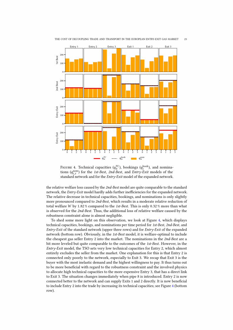
the relative welfare loss caused by the 2nd-Best model are quite comparable to the standardnetwork, the Entry-Exit model hardly adds further ine�ciencies for the expanded network.The relative decrease in technical capacities, bookings, and nominations is only slightlymore pronounced compared to 2nd-Best, which results in a moderate relative reduction oftotal welfareW by 1.82 % compared to the 1st-Best. This is only 0.32 % more than whatis observed for the 2nd-Best. Thus, the additional loss of relative welfare caused by therobustness constraint alone is almost negligible.
To shed some more light on this observation, we look at Figure 4, which displaystechnical capacities, bookings, and nominations per time period for 1st-Best, 2nd-Best, andEntry-Exit of the standard network (upper three rows) and for Entry-Exit of the expandednetwork (bottom row). Obviously, in the 1st-Best model, it is welfare-optimal to includethe cheapest gas seller Entry 2 into the market. The nominations in the 2nd-Best are abit more leveled but quite comparable to the outcomes of the 1st-Best. However, in theEntry-Exit model, the TSO sets very low technical capacities for Entry 2, which almostentirely excludes the seller from the market. One explanation for this is that Entry 2 isconnected only poorly to the network, especially to Exit 3. We recap that Exit 3 is thebuyer with the most inelastic demand and the highest willingness to pay. It thus turns outto be more bene�cial with regard to the robustness constraint and the involved physicsto allocate high technical capacities to the more expensive Entry 3, that has a direct linkto Exit 3. The situation changes immediately when pipe 8 is introduced. Entry 2 is nowconnected better to the network and can supply Exits 1 and 2 directly. It is now bene�cialto include Entry 2 into the trade by increasing its technical capacities; see Figure 4 (bottomrow).

24 T. BÖTTGER, V. GRIMM, T. KLEINERT, M. SCHMIDT
The discussion in this section indicates that the network con�guration strongly impactsthe market outcomes of the individual players. In this light, trade and transport are notdecoupled after all, which is most obvious in the setting of the standard network, where itis welfare-optimal to exclude the cheapest producer from the market. The results of thissection also indicate that in more expanded networks, the cost of decoupling trade andtransport is rather small. This low cost however comes at the expense of possibly highinvestment costs for building and maintaining an (over-)expanded network.
Finally note that, in this section, we just compared the e�ciency losses from an Entry-Exit model as compared to the 1st-Best and 2nd-Best for di�erent network con�gurations.The network design problem that would have to be solved in order to set up the networkoptimally cannot be addressed in this paper. Obviously, one would have to account forthe costs and bene�ts of adding pipes, accounting for all endogenous feedback e�ects ofnetwork expansion on the market outcome.
6.5. The E�ect of Di�erent Pricing Regimes. In the last two sections, we have seenthat entry-exit-like systems can cause severe reductions in total welfareW compared tothe 1st-Best and 2nd-Best models. This cost of decoupling trade and transport is “payed”by the gas buying and selling �rms by decreasing rents. However, in general, this costwill not be shared equally but some players may be discriminated by the market system,while others may even bene�t from the decoupling of trade and transport.
In this section, we analyze how the individual rents
Ri =∑t ∈T
(πnomt − cvar
i )qnomi ,t − ¯
π booku qbook
i , i ∈ Pu , u ∈ V+,
Ri =∑t ∈T
(Pi ,t (qnomi ,t ) − π
nomt )qnom
i ,t − ¯π booku qbook
i , i ∈ Pu , u ∈ V−
are a�ected by entry-exit-like systems. The two equations above represent the buyers’and the sellers’ rents, respectively. Note that the price �oor
¯π booku , that is set by the TSO to
recover transportation and exogenous network costs (cf. Constraint (1c)), directly impactsthe individual rents of the players. The price �oors can be chosen by the TSO in variousways. In this section, we analyze four di�erent such pricing regimes: (i) a regime in whichprice �oors are chosen e�ciently, (ii) a regime with a single uniform booking price �oor atall entry and exit nodes, (iii) a regime in which only exit nodes pay a uniform bookingprice �oor, and (iv) a regime in which only entry nodes pay a uniform booking price �oor.Note that (i) is assumed implicitly for our modeling in Section 2 and that the other threeregimes can be modeled by additional linear constraints. To better illustrate the e�ects ofthe various pricing schemes we use exogenously given network costs of C = 300 000 EURthroughout this section. This high value of the investment costs, which must be earnedvia the price �oors (cf. Constraint (1c)), allows to illustrate the e�ect of the price �oorson e�ciency very clearly. Since the comparison between the di�erent market designs inthe previous sections is not enriched by this assumption about investment costs, we havenot speci�ed the costs there. Note further that we use the standard network without thedashed pipe 8, see Figure 3, in this subsection.
Table 5 displays the reduction in total welfareW as compared to the 1st-Best model foreach of the four di�erent pricing regimes and shows how the rents Ri of all gas sellers andbuyers are a�ected. All values represent absolute reductions in comparison to the welfareand rents achieved in the 1st-Best model, which is the same for all four pricing regimes.In addition, Figure 5 shows the welfare-maximizing price �oors
¯π booku and payments
¯π booku qbook
i for the four pricing schemes. At a �rst glance, the di�erent pricing regimesyield diverse price �oor patterns, see Figure 5, which is not surprising. Also, the totalwelfare is a�ected by the choice of the pricing scheme; see Table 5. Of course, the e�cientpricing scheme yields the lowest reduction of welfare compared to the 1st-Best because itshifts payments to agents where they do not induce welfare losses. The same welfare result

THE COST OF DECOUPLING TRADE AND TRANSPORT IN THE EUROPEAN ENTRY-EXIT GAS MARKET 25
Table 5. Absolute reduction (in 1000 EUR) of rents Ri and total wel-fareW compared to the 1st-Best model for di�erent pricing regimes.
Reduction Entry 1 Entry 2 Entry 3 Exit 1 Exit 2 Exit 3 Win 1000 EUR
E�cient 41.87 41.87 −181.11 122.48 148.41 7.35 180.86Uniform −36.28 38.94 −113.44 143.75 153.33 0.66 186.96Only Exit −35.43 39.02 −109.22 142.17 154.53 −1.74 189.33Only Entry −19.62 39.58 −76.63 122.48 148.41 −33.35 180.86
Entry 1 Entry 2 Entry 3 Exit 1 Exit 2 Exit 3
0
200
400
600
800
1000
1200
1400¯π book
u in EUR/(1000 Nm3/h)
Entry 1 Entry 2 Entry 3 Exit 1 Exit 2 Exit 3
0
50000
100000
150000
200000
¯π book
u · qbooki in EUR
E�icient Uniform Only Exit Only Entry
Figure 5. Comparison of price �oors (left) and products of price �oorstimes bookings (right) for the pricing regimes e�cient, uniform, onlyexit, and only entry.
can be obtained by charging price �oors for entries only, since obviously those paymentsdo not induce any e�ect on the quantity supplied at the market. As long as revenues of gassellers are high enough, the TSO can collect his expenses for gas transportation and otherexogenous network costs from the sellers. The fact that Exit 3 receives a price �oor ofaround 200 EUR/(1000Nm3/h) in the e�cient pricing scheme compared to a price �oor of0 EUR/(1000Nm3/h) in the only entry pricing scheme is an artifact of non-unique welfare-maximizing price �oors. In particular, the only entry pricing scheme, which charges thesame price �oor at every entry node, is also a feasible e�cient pricing scheme. It can alsobe seen in Table 5 that imposing price �oors for exit players like it is done in the pricingregimes uniform and only exit results in additional welfare losses. This is due to the factthat the players’ marginal units are driven out of the market at Exit 1 and 2 if a bookingfee is charged. We now take a closer look at the implications for the individual players.
From Table 5 it can be seen that Entry 2 is not a�ected much by changes in the pricingscheme. The rent of Entry 2 is reduced by around 42 000 EUR compared to the 1st-Bestunder the e�cient pricing scheme. This reduction decreases slightly, when other pricingschemes are used. As seen in the previous sections, the reason is the following. SinceEntry 2 is the cheapest seller, it is assigned as much nomination qnom
i as possible withrespect to physics in the 1st-Best model; cf. Figure 4. However, due to its poor networkaccess in combination with the robustness constraint of the entry-exit system, Entry 2 isexcluded from the market by having its technical capacities set to zero by the TSO. Thus,the high price �oor that Entry 2 receives is irrelevant and the contribution
¯π booku qbook
iof Entry 2 to the reimbursement of the TSO for transportation and network expenses ismarginal; see Figure 5 (right). A direct consequence is that the rent of Entry 3 increasescompared to the 1st-Best throughout all pricing schemes. The amount that Entry 1 sells in1st-Best but not in Entry-Exit is compensated by Entry 3. In the e�cient pricing scheme,
26 T. BÖTTGER, V. GRIMM, T. KLEINERT, M. SCHMIDT
this results in an increase of the rent of Entry 3 of 181 110 EUR compared to the 1st-Best,which is signi�cant, taking into account that the reduction of total welfare amounts to180 860 EUR. In the e�cient pricing scheme, the increasing rent of Entry 3 is in parts atthe expense of Entry 1, whose rent is reduced by around 42 000 EUR compared to the �rstbest. This reduction is also caused by a very high price �oor that is set by the TSO. It isinteresting to see that in the e�cient pricing scheme, the highest contribution to cover theexpenses of the TSO comes from Entry 1; see Figure 5 (right). The reason is that at Entry 1the expenses of the TSO can be recovered with the least distorting e�ects. Note also thatEntry 2 seems to be charged a high fee but in e�ect pays nothing since the entry receivesno bookable capacity. Using any other pricing scheme than e�cient immediately yields anincreasing rent of Entry 1, since the burden is shifted also to other agents. However, thishappens at a cost, in case trade is suppressed.
Similar observations can be drawn when looking at the exit players. Exits 1 and 2 do notreceive a price �oor in the e�cient and (obviously) in the only entry pricing regime. Thus,these two regimes yield the lowest rent reduction for the two exits. Still, the reductionis, compared to the 1st-Best and the reduction of total welfareW , very signi�cant. Thisis not the case for Exit 3 in the e�cient pricing regime. Since the demand of Exit 3 isvery inelastic, the reduction of the rent compared to the 1st-Best is rather low. The renteven increases compared to the 1st-Best, when only the entries are charged with a price�oor. It is also noteworthy that the uniform and only exit pricing regimes increase therent of Exit 3 compared to the e�cient regime, although the former two regimes yieldsigni�cantly higher booking price �oors and booking payments for Exit 3; see Figure 5.The reason is that Exit 3 can realize higher nominations, which overcompensates theincreasing payments.
From the analysis in this section, we can draw several conclusions. The actual choiceof the pricing regime for booking price �oors can a�ect both, the total welfare as wellas the individual rents, and can add to the cost of decoupling trade and transport. Thee�cient booking price �oor regime yields the best overall welfare outcome but is highlydiscriminating in the sense that the rent of Entry 3 increases drastically at the expense ofall other players. The regime only entry yields the same welfare outcome but distributesthe reductions of the rents way more evenly. This makes also clear that in all thoseconsiderations one has to account for the fact that the Entry-Exit model might havemultiple solutions.
7. Conclusion
In this paper, we analyzed ine�ciencies that arise in entry-exit gas markets due tothe decoupling of trade and transport. To this end, we used an existing multilevel modelof the European entry-exit system and an equivalent bilevel reformulation thereof fromthe literature [24]. We reformulated this bilevel problem as an equivalent nonconvexand nonsmooth mixed-integer single-level problem. The major di�culty of the single-level problem is an entry-exit-market speci�c robustness constraint that directly resultsfrom a proper modeling of the underlying gas market system: The TSO needs to ensurethat every balanced nomination that is feasible w.r.t. technical capacities is transportable.This constraint alone renders the problem intractable in general. However, under theassumption of passive networks (i.e., without active elements such as compressor stations),and a potential-based but linear �ow model, we derived a “more tractable” single-levelreformulation by applying a characterization of the feasible points of the robustnessconstraint from [39].
In a case study for a stylized network, we analyzed the ine�ciencies caused by entry-exit systems and identi�ed four major e�ects. First, the robustness constraint accountsfor signi�cant welfare losses compared to �rst-best and second-best models. This meansthat—under the assumptions made—the cost of decoupling trade and transport can indeed
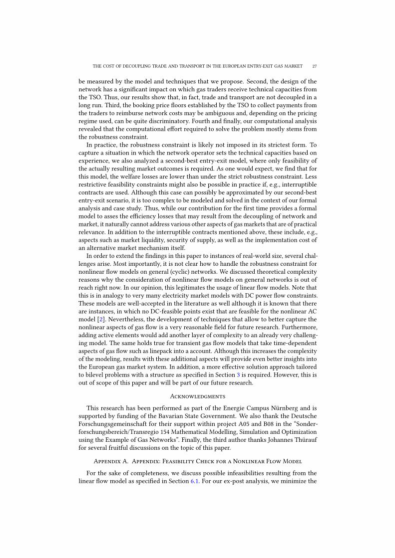
THE COST OF DECOUPLING TRADE AND TRANSPORT IN THE EUROPEAN ENTRY-EXIT GAS MARKET 27
be measured by the model and techniques that we propose. Second, the design of thenetwork has a signi�cant impact on which gas traders receive technical capacities fromthe TSO. Thus, our results show that, in fact, trade and transport are not decoupled in along run. Third, the booking price �oors established by the TSO to collect payments fromthe traders to reimburse network costs may be ambiguous and, depending on the pricingregime used, can be quite discriminatory. Fourth and �nally, our computational analysisrevealed that the computational e�ort required to solve the problem mostly stems fromthe robustness constraint.
In practice, the robustness constraint is likely not imposed in its strictest form. Tocapture a situation in which the network operator sets the technical capacities based onexperience, we also analyzed a second-best entry-exit model, where only feasibility ofthe actually resulting market outcomes is required. As one would expect, we �nd that forthis model, the welfare losses are lower than under the strict robustness constraint. Lessrestrictive feasibility constraints might also be possible in practice if, e.g., interruptiblecontracts are used. Although this case can possibly be approximated by our second-bestentry-exit scenario, it is too complex to be modeled and solved in the context of our formalanalysis and case study. Thus, while our contribution for the �rst time provides a formalmodel to asses the e�ciency losses that may result from the decoupling of network andmarket, it naturally cannot address various other aspects of gas markets that are of practicalrelevance. In addition to the interruptible contracts mentioned above, these include, e.g.,aspects such as market liquidity, security of supply, as well as the implementation cost ofan alternative market mechanism itself.
In order to extend the �ndings in this paper to instances of real-world size, several chal-lenges arise. Most importantly, it is not clear how to handle the robustness constraint fornonlinear �ow models on general (cyclic) networks. We discussed theoretical complexityreasons why the consideration of nonlinear �ow models on general networks is out ofreach right now. In our opinion, this legitimates the usage of linear �ow models. Note thatthis is in analogy to very many electricity market models with DC power �ow constraints.These models are well-accepted in the literature as well although it is known that thereare instances, in which no DC-feasible points exist that are feasible for the nonlinear ACmodel [2]. Nevertheless, the development of techniques that allow to better capture thenonlinear aspects of gas �ow is a very reasonable �eld for future research. Furthermore,adding active elements would add another layer of complexity to an already very challeng-ing model. The same holds true for transient gas �ow models that take time-dependentaspects of gas �ow such as linepack into a account. Although this increases the complexityof the modeling, results with these additional aspects will provide even better insights intothe European gas market system. In addition, a more e�ective solution approach tailoredto bilevel problems with a structure as speci�ed in Section 3 is required. However, this isout of scope of this paper and will be part of our future research.
Acknowledgments
This research has been performed as part of the Energie Campus Nürnberg and issupported by funding of the Bavarian State Government. We also thank the DeutscheForschungsgemeinschaft for their support within project A05 and B08 in the “Sonder-forschungsbereich/Transregio 154 Mathematical Modelling, Simulation and Optimizationusing the Example of Gas Networks”. Finally, the third author thanks Johannes Thürauffor several fruitful discussions on the topic of this paper.
Appendix A. Appendix: Feasibility Check for a Nonlinear Flow Model
For the sake of completeness, we discuss possible infeasibilities resulting from thelinear �ow model as speci�ed in Section 6.1. For our ex-post analysis, we minimize the

28 T. BÖTTGER, V. GRIMM, T. KLEINERT, M. SCHMIDT
Table 6. Results of the nonlinear �ow feasibility check.
Instance Model # Viol. Total Viol. Max. Viol. At Node
6 Nodes 1st-Best 10 210.5 34.1 Entry 16 Nodes 2nd-Best 6 62.7 24.3 Entry 36 Nodes Entry-Exit 11 104.2 17.4 Entry 36 Nodes, Low Demand 1st-Best 8 149.7 34.8 Entry 16 Nodes, Low Demand 2nd-Best 7 101.2 19.6 Entry 36 Nodes, Low Demand Entry-Exit 2 10.0 6.6 Entry 36 Nodes, High Demand 1st-Best 14 249.5 24.7 Entry 16 Nodes, High Demand 2nd-Best 11 153.4 20.5 Exit 36 Nodes, High Demand Entry-Exit 6 68.9 15.9 Exit 36 Nodes, Extended 1st-Best 6 94.4 20.2 Exit 36 Nodes, Extended 2nd-Best 2 36.8 20.7 Entry 36 Nodes, Extended Entry-Exit 2 28.9 16.9 Exit 36 Nodes, Network Investment 1st-Best 10 210.5 34.1 Entry 16 Nodes, Network Investment 2nd-Best 5 61.2 24.3 Entry 36 Nodes, Network Investment Entry-Exit 11 104.2 17.4 Entry 36 Nodes, Uniform Price�oor 2nd-Best 6 57.5 24.6 Entry 36 Nodes, Uniform Price�oor Entry-Exit 7 72.8 16.7 Entry 36 Nodes, Only Entry Price�oor 2nd-Best 6 62.9 24.3 Entry 36 Nodes, Only Entry Price�oor Entry-Exit 11 104.2 17.4 Entry 36 Nodes, Only Exit Price�oor 2nd-Best 6 57.5 24.6 Entry 36 Nodes, Only Exit Price�oor Entry-Exit 10 82.9 15.5 Entry 39 Nodes 1st-Best 15 293.3 34.2 Entry 49 Nodes 2nd-Best 4 53.6 23.0 Entry 39 Nodes Entry-Exit 6 62.9 18.2 Entry 3
sum of squared pressure bound violations, i.e., we solve the nonlinear problem
minπ ,q,s−,s+
∑t ∈T
∑u ∈V
(s−u ,t + s
+u ,t
)s.t. (5)–(7),
π−u − s−u ,t ≤ πu ,t ≤ π
+u ≤ +s
+u ,t for all u ∈ V , t ∈ T ,
s−u ,t , s+u ,t ≥ 0 for all u ∈ V , t ∈ T ,
in which the nominations qnomi ,t are �xed to the solution provided by our solution approach.
As a solver, we used the local solver CONOPT4. We also checked for some exemplaryinstances with the global solver BARON, if the solution provided by CONOPT4 is a globaloptimum. For all our tests, this was the case. In Table 6, we summarize the results for allinstances that we used throughout this paper. The �rst two columns specify the instance.The third column lists the number of pressure bound violations (over all nodes in thenetwork and over all time periods), whereas the fourth column lists the aggregated boundviolation and the �fth one lists the maximum violation. The last column denotes the nodein the network at which the largest violation occurred.
References
[1] Alonso, A., Olmos, L., and Serrano, M. “Application of an entry–exit tari� model tothe gas transport system in Spain.” In: Energy Policy 38.5 (2010), pp. 5133–5140. doi:10.1016/j.enpol.2010.04.043.
[2] Baker, K. Solutions of DC OPF are Never AC Feasible. Tech. rep. 2020. url: https://arxiv.org/pdf/1912.00319.pdf.

REFERENCES 29
[3] Baltensperger, T., Füchslin, R. M., Krütli, P., and Lygeros, J. “Multiplicity of equilibriain conjectural variations models of natural gas markets.” In: European Journal ofOperational Research 252.2 (2016), pp. 646–656. doi: 10.1016/j.ejor.2016.01.032.
[4] Ben-Tal, A., El Ghaoui, L., and Nemirovski, A. Robust Optimization. Princeton Uni-versity Press, 2009.
[5] Ben-Tal, A., Goryashko, A., Guslitzer, E., and Nemirovski, A. “Adjustable robustsolutions of uncertain linear programs.” In: Mathematical Programming 99.2 (2004),pp. 351–376. doi: 10.1007/s10107-003-0454-y.
[6] Bertsimas, D., Brown, D. B., and Caramanis, C. “Theory and Applications of Ro-bust Optimization.” In: SIAM Review 53.3 (2011), pp. 464–501. doi: 10.1137/080734510.
[7] Boots, M. G., Rijkers, F. A., and Hobbs, B. F. “Trading in the Downstream EuropeanGas Market: A Successive Oligopoly Approach.” In: The Energy Journal 25.3 (2004),pp. 73–102. url: http://www.jstor.org/stable/41323043.
[8] Boucher, J. and Smeers, Y. “Economic forces in the European gas market — a 1985prospective.” In: Energy Economics 9.1 (1987), pp. 2–16. doi: 10.1016/0140-9883(87)90002-8.
[9] Boucher, J. and Smeers, Y. “Gas trade in the European community during the 1970s.”In: Energy Economics 7.2 (1985), pp. 102–116. doi: 10.1016/0140-9883(85)90025-8.
[10] Boyd, S. and Vandenberghe, L. Convex Optimization. Cambridge University Press,2004. doi: 10.1017/cbo9780511804441.
[11] Chyong, C. K. and Hobbs, B. F. “Strategic Eurasian natural gas market model forenergy security and policy analysis: Formulation and application to South Stream.”In: Energy Economics 44 (2014), pp. 198–211. doi: 10.1016/j.eneco.2014.04.006.
[12] Cremer, H. and La�ont, J.-J. “Competition in gas markets.” In: European EconomicReview 46.4–5 (2002), pp. 928–935. doi: 10.1016/S0014-2921(01)00226-4.
[13] Egging, R., Gabriel, S. A., Holz, F., and Zhuang, J. “A complementarity model forthe European natural gas market.” In: Energy Policy 36.7 (2008), pp. 2385–2414. doi:10.1016/j.enpol.2008.01.044.
[14] Egging, R., Holz, F., and Gabriel, S. A. “The World Gas Model: A multi-period mixedcomplementarity model for the global natural gas market.” In: Energy 35.10 (2010),pp. 4016–4029. doi: 10.1016/j.energy.2010.03.053.
[15] European Parliament and Council of the European Union. Directive 2003/55/EC ofthe European Parliament and of the Council of 26 June 2003 concerning common rulesfor the internal market in natural gas and repealing Directive 98/30/EC. 2003.
[16] European Parliament and Council of the European Union. Directive 2009/73/EC ofthe European Parliament and of the Council concerning common rules for the internalmarket in natural gas and repealing Directive 2003/55/EC. 2009.
[17] European Parliament and Council of the European Union. Directive 98/30/EC of theEuropean Parliament and of the Council of 22 June 1998 concerning common rules forthe internal market in natural gas. 1998.
[18] Fischetti, M., Ljubić, I., Monaci, M., and Sinnl, M. “A New General-Purpose Algorithmfor Mixed-Integer Bilevel Linear Programs.” In: Operations Research 65.6 (2017),pp. 1615–1637. doi: 10.1287/opre.2017.1650.
[19] Fortuny-Amat, J. and McCarl, B. “A Representation and Economic Interpretationof a Two-Level Programming Problem.” In: The Journal of the Operational ResearchSociety 32.9 (1981), pp. 783–792. JSTOR: 2581394.

30 REFERENCES
[20] Fügenschuh, A., Geißler, B., Gollmer, R., Morsi, A., Pfetsch, M. E., Rövekamp, J.,Schmidt, M., Spreckelsen, K., and Steinbach, M. C. “Physical and technical funda-mentals of gas networks.” In: Evaluating Gas Network Capacities. Ed. by T. Koch,B. Hiller, M. E. Pfetsch, and L. Schewe. SIAM-MOS series on Optimization. SIAM,2015. Chap. 2, pp. 17–44. doi: 10.1137/1.9781611973693.ch2.
[21] Gabriel, S. A., Kiet, S., and Zhuang, J. “A Mixed Complementarity-Based EquilibriumModel of Natural Gas Markets.” In: Operations Research 53.5 (2005), pp. 799–818. doi:10.1287/opre.1040.0199.
[22] Glachant, J.-M., Hallack, M., and Vazquez, M. Building Competitive Gas Markets inthe EU. Cheltenham: Edward Elgar Publishing, 2013.
[23] Grimm, V., Grübel, J., Schewe, L., Schmidt, M., and Zöttl, G. “Nonconvex equilibriummodels for gas market analysis: Failure of standard techniques and alternativemodeling approaches.” In: European Journal of Operational Research 273.3 (2019),pp. 1097–1108. doi: 10.1016/j.ejor.2018.09.016.
[24] Grimm, V., Schewe, L., Schmidt, M., and Zöttl, G. “A Multilevel Model of the Euro-pean Entry-Exit Gas Market.” In: Mathematical Methods of Operations Research 89.2(2019), pp. 223–255. doi: 10.1007/s00186-018-0647-z.
[25] Groß, M., Pfetsch, M. E., Schewe, L., Schmidt, M., and Skutella, M. “Algorithmicresults for potential-based �ows: Easy and hard cases.” In: Networks (2019). doi:10.1002/net.21865.
[26] Hallack, M. and Vazquez, M. “European Union Regulation of Gas TransmissionServices: Challenges in the Allocation of Network Resources through Entry/exitSchemes.” In: Utilities Policy 25 25.5 (2013), pp. 23–32. doi: 10.1016/j.jup.2013.01.003.
[27] Hansen, P., Jaumard, B., and Savard, G. “New branch-and-bound rules for linearbilevel programming.” In: SIAM Journal on Scienti�c and Statistical Computing 13.5(1992), pp. 1194–1217. doi: 10.1137/0913069.
[28] Hirschhausen, C. “Reform der Erdgaswirtschaft in der EU und in Deutschland:Wieviel Regulierung braucht der Wettbewerb?” In: Perspektiven der Wirtschaftspoli-tik 7.1 (2006), pp. 89–103. doi: 10.1111/j.1465-6493.2006.00200.x.
[29] Holz, F., Hirschhausen, C. von, and Kemfert, C. “A strategic model of European gassupply (GASMOD).” In: Energy Economics 30.3 (2008), pp. 766–788. doi: 10.1016/j.eneco.2007.01.018.
[30] Hunt, P. Entry-Exit transmission pricing with national hubs. Can it deliver a Pan-European wholesale market in gas? Tech. rep. Oxford Institute of Energy Studies,2008.
[31] Huppmann, D. “Endogenous production capacity investment in natural gas marketequilibrium models.” In: European Journal of Operational Research 231.2 (2013),pp. 503–506. doi: 10.1016/j.ejor.2013.05.048.
[32] Ikonnikova, S. and Zwart, G. T. “Trade quotas and buyer power, with an applicationto the E.U. natural gas market.” In: Journal of the European Economic Association12.1 (2014), pp. 177–199. doi: 10.1111/jeea.12064.
[33] Jansen, T., Lier, A. van, Witteloostuijn, A. van, and Ochssée, T. B. von. “A modi�edCournot model of the natural gas market in the European Union: Mixed-motivesdelegation in a politicized environment.” In: Energy Policy 41 (2012). ModelingTransport (Energy) Demand and Policies, pp. 280–285. doi: 10.1016/j.enpol.2011.10.047.
[34] Jeroslow, R. G. “The polynomial hierarchy and a simple model for competitiveanalysis.” In: Mathematical Programming 32.2 (1985), pp. 146–164. doi: 10.1007/BF01586088.

REFERENCES 31
[35] Kleinert, T., Grimm, V., and Schmidt, M. Outer Approximation for Global Optimizationof Mixed-Integer Quadratic Bilevel Problems. Tech. rep. 2020. url: http://www.optimization-online.org/DB_FILE/2019/12/7534.pdf.
[36] Kleinert, T., Labbé, M., Plein, F., and Schmidt, M. “There’s No Free Lunch: On theHardness of Choosing a Correct Big-M in Bilevel Optimization.” In: OperationsResearch (2019). url: http://www.optimization-online.org/DB_HTML/2019/04/7172.html. Forthcoming.
[37] Kleinert, T. and Schmidt, M. “Global Optimization of Multilevel Electricity MarketModels Including Network Design and Graph Partitioning.” In: Discrete Optimization33 (2019), pp. 43–69. doi: 10.1016/j.disopt.2019.02.002.
[38] Koch, T., Hiller, B., Pfetsch, M. E., and Schewe, L. Evaluating Gas Network Ca-pacities. SIAM-MOS series on Optimization. SIAM, 2015. doi: 10 . 1137 / 1 .9781611973693.
[39] Labbé, M., Plein, F., and Schmidt, M. “Bookings in the European Gas Market: Char-acterisation of Feasibility and Computational Complexity Results.” In: Optimizationand Engineering 21.1 (2020), pp. 305–334. doi: 10.1007/s11081-019-09447-0.
[40] Lozano, L. and Smith, J. C. “A value-function-based exact approach for the bilevelmixed-integer programming problem.” In: Operations Research 65.3 (2017), pp. 768–786. doi: 10.1287/opre.2017.1589.
[41] McCormick, G. P. “Computability of global solutions to factorable nonconvex pro-grams: Part I—Convex underestimating problems.” In: Mathematical Programming10.1 (1976), pp. 147–175. doi: 10.1007/BF01580665.
[42] Meran, G., Hirschhausen, C. von, and Neumann, A. “Access Pricing and NetworkExpansion in Natural Gas Markets.” In: Zeitschrift für Energiewirtschaft 34.3 (2010),pp. 179–183. doi: 10.1007/s12398-010-0028-7.
[43] Midthun, K. T., Bjorndal, M., and Tomasgard, A. “Modeling Optimal EconomicDispatch and System E�ects in Natural Gas Networks.” In: The Energy Journal 30.4(2009), pp. 155–180. url: https://ideas.repec.org/a/aen/journl/2009v30-04-a06.html.
[44] Midthun, K. T., Fodstad, M., and Hellemo, L. “Optimization Model to Analyse OptimalDevelopment of Natural Gas Fields and Infrastructure.” In: Energy Procedia 64 (2015),pp. 111–119. doi: 10.1016/j.egypro.2015.01.014.
[45] Moore, J. T. and Bard, J. F. “The mixed integer linear bilevel programming problem.”In: Operations Research 38.5 (1990), pp. 911–921. doi: 10.1287/opre.38.5.911.
[46] Oliver, M. E., Mason, C. F., and Finno�, D. “Pipeline congestion and basis di�eren-tials.” In: Journal of Regulatory Economics 46.3 (2014), pp. 261–291. doi: 10.1007/s11149-014-9256-9.
[47] Pineda, S. and Morales, J. M. “Solving Linear Bilevel Problems Using Big-Ms: NotAll That Glitters Is Gold.” In: IEEE Transactions on Power Systems (2019). doi: 10.1109/TPWRS.2019.2892607.
[48] Regionales Rechenzentrum Erlangen. Woodcrest Cluster. url: https://www.anleitungen . rrze . fau . de / hpc / woody - cluster/ (visited on06/18/2020).
[49] Rømo, F., Tomasgard, A., Hellemo, L., Fodstad, M., Eidesen, B. H., and Pedersen, B.“Optimizing the Norwegian Natural Gas Production and Transport.” In: Interfaces39.1 (2009), pp. 46–56. doi: 10.1287/inte.1080.0414.
[50] Siddiqui, S. and Gabriel, S. A. “Modeling market power in the U.S. shale gas market.”In: Optimization and Engineering 18.1 (2017), pp. 203–213. doi: 10.1007/s11081-016-9310-9.
[51] Smeers, Y. Gas models and three di�cult objectives. Tech. rep. Core Discussion Paper,2008. url:http://www.uclouvain.be/cps/ucl/doc/core/documents/coreDP2008_9.pdf.

32 REFERENCES
[52] Vazquez, M., Hallack, M., and Glachant, J.-M. “Designing the European Gas Market:More Liquid and Less Natural?” In: Economics of Energy and Environmental Policy1.3 (2012). doi: 10.5547/2160-5890.1.3.3.
[53] Vielma, J. P., Ahmed, S., and Nemhauser, G. “Mixed-integer models for nonseparablepiecewise-linear optimization: Unifying framework and extensions.” In: OperationsResearch 58.2 (2010), pp. 303–315. doi: 10.1287/opre.1090.0721.
[54] Weymouth, T. R. “Problems in Natural Gas Engineering.” In: Trans. Amer. Soc. ofMech. Eng. 34.1349 (1912), pp. 185–231.
[55] Xu, P. and Wang, L. “An exact algorithm for the bilevel mixed integer linear program-ming problem under three simplifying assumptions.” In: Computers & OperationsResearch 41 (2014), pp. 309–318. doi: 10.1016/j.cor.2013.07.016.
[56] Yang, Z., Zhang, R., and Zhang, Z. “An exploration of a strategic competition modelfor the European Union natural gas market.” In: Energy Economics 57 (2016), pp. 236–242. doi: 10.1016/j.eneco.2016.05.008.
[57] Yanıkoğlu, İ., Gorissen, B., and Hertog, D. den. “A Survey of Adjustable RobustOptimization.” In: European Journal of Operational Research 277.3 (2019), pp. 799–813. doi: 10.1016/j.ejor.2018.08.031.
[58] Zare, M. H., Borrero, J. S., Zeng, B., and Prokopyev, O. A. “A note on linearizedreformulations for a class of bilevel linear integer problems.” In: Annals of OperationsResearch 272.1-2 (2019), pp. 99–117. doi: 10.1007/s10479-017-2694-x.
[59] Zwart, G. and Mulder, M. NATGAS: a model of the European natural gas market.Tech. rep. 144. CPB Netherlands Bureau for Economic Policy Analysis, 2006. url:https://ideas.repec.org/p/cpb/memodm/144.html.
(T. Böttger) Friedrich-Alexander-Universität Erlangen-Nürnberg (FAU), Discrete Optimization,Cauerstr. 11, 91058 Erlangen, Germany
Email address: [email protected]
(V. Grimm) (A) Friedrich-Alexander-Universität Erlangen-Nürnberg (FAU), Economic Theory, LangeGasse 20, 90403 Nürnberg, Germany; (B) Energie Campus Nürnberg, Fürther Str. 250, 90429 Nürnberg,Germany
Email address: [email protected]
(T. Kleinert) (A) Friedrich-Alexander-Universität Erlangen-Nürnberg (FAU), Discrete Optimization,Cauerstr. 11, 91058 Erlangen, Germany; (B) Friedrich-Alexander-Universität Erlangen-Nürnberg(FAU), Economic Theory, Lange Gasse 20, 90403 Nürnberg, Germany; (C) Energie Campus Nürnberg,Fürther Str. 250, 90429 Nürnberg, Germany
Email address: [email protected]
(M. Schmidt) Trier University, Department of Mathematics, Universitätsring 15, 54296 Trier,Germany
Email address: [email protected]