The Cost of Climate Change: What We'll Pay if Global Warming

Blank Page i

May 2008 The Cost of Climate Change

What We’ll Pay if Global Warming Continues Unchecked

AuthorsFrank Ackerman and Elizabeth A. StantonGlobal Development and Environment Institute and Stockholm Environment Institute-US Center, Tufts University

Contributing AuthorsChris Hope and Stephan AlberthJudge Business School, Cambridge University

Jeremy Fisher and Bruce BiewaldSynapse Energy Economics

Project ManagersElizabeth Martin Perera, Natural Resources Defense CouncilDan Lashof, Natural Resources Defense Council

The Cost of Climate Change: What We’ll Pay if Global Warming Continues Unchecked

ii

About NRDC NRDC (Natural Resources Defense Council) is a national nonprofit environmental organization with more than 1.2 million members and online activists. Since 1970, our lawyers, scientists, and other environmental specialists have worked to protect the world’s natural resources, public health, and the environment. NRDC has offices in New York City, Washington, D.C., Los Angeles, San Francisco, Chicago, and Beijing. Visit us at www.nrdc.org.

Acknowledgments The authors and project managers would like to thank our peer reviewers, Dr. Matthias Ruth, Professor of Public Policy at the University of Maryland, and Rick Duke, Director of the Center for Market Innovation at NRDC. NRDC would also like to thank Sea Change Foundation, The Streisand Foundation, The William and Flora Hewlett Foundation, The Energy Foundation, Public Welfare Foundation, and Wallace Genetic Foundation, Inc. for their generous support.

NRDC Director of Communications: Phil GutisNRDC Marketing and Operations Director: Alexandra KennaughNRDC Publications Manager: Lisa GoffrediNRDC Publications Editor: Anthony Clark

Copyright 2008 Natural Resources Defense Council.

For additional copies of this report, send $5.00 plus $3.95 shipping and handling to NRDC Publications Department, 40 West 20th Street, New York, NY 10011. California residents must add 7.5% sales tax. Please make checks payable to NRDC in U.S. dollars. The report is also available online at www.nrdc.org/policy.

This report is printed on paper that is 100 percent post-consumer recycled fiber, processed chlorine free.

iii

Table of Contents

Executive Summary iv

Chapter 1: The Global Warming Price Tag Under Business-as-Usual Emissions 1

Chapter 2: More Intense Hurricanes Cause Financial Damage 5

Chapter 3: Real Estate Losses as a Result of Sea Level Rise 7

Chapter 4: Costly Changes to the Energy Sector 9

Chapter 5: Water and Agriculture Hit Hard by Global Warming 15

Chapter 6: Modeling U.S. Climate Impacts: Beyond the Stern Review 19

Chapter 7: Conclusion 25

Chapter 8: NRDC's Policy Recommendations 26

Endnotes 29

Appendix: A State-by-State Analysis of Warming in the West 41

iv

Executive Summary

Global warming comes with a big price tag for every country around the

world. The 80 percent reduction in U.S. emissions that will be needed to

lead international action to stop climate change may not come cheaply,

but the cost of failing to act will be much greater. New research shows that if present

trends continue, the total cost of global warming will be as high as 3.6 percent of gross

domestic product (GDP). Four global warming impacts alone—hurricane damage,

real estate losses, energy costs, and water costs—will come with a price tag of 1.8

percent of U.S. GDP, or almost $1.9 trillion annually (in today’s dollars) by 2100. We

know how to avert most of these damages through strong national and international

action to reduce the emissions that cause global warming. But we must act now. The

longer we wait, the more painful—and expensive—the consequences will be.

This report focuses on a “business-as-usual” future in which the world continues to emit heat-trapping gases at an increasing rate. We base our economic projections on the most pessimistic of the business-as-usual climate forecasts considered “likely” by the scientific community.1 In this projected climate future, which is still far from the worst case scenario, global warming causes drastic changes to the planet’s climate, with average temperature increases of 13 degrees Fahrenheit in most of the United States and 18 degrees Fahrenheit in Alaska over the next 100 years. The effects of climate change will be felt in the form of more severe heat waves, hurricanes, droughts, and other erratic weather events—and in their impact on our economy’s bottom line.

We estimate U.S. economic impacts from global warming in two ways: a detailed focus on four specific impacts and a comprehensive look at the costs to the country as a whole. Our detailed accounting of costs begins with historical data for four especially important climate impacts: hurricane damages, real estate losses,

energy costs, and water costs. We then build upward to estimate the impact of future climatic conditions in these four impact areas. The second part of our analysis is a comprehensive view of climate change impacts: we take a general rule about how the climate affects the country as a whole and then apply that rule to business-as-usual climate forecasts. Although the detailed impact studies can provide only a partial accounting of the full economic costs estimated by our comprehensive model, the impact studies allow us to examine the costs of climate change with greater specificity for the particular case of the United States.

Putting a Price Tag on Global WarmingDroughts, floods, wildfires, and hurricanes have already caused multibillion-dollar losses, and these extreme weather events will likely become more frequent and more devastating as the climate continues to change. Tourism, agriculture, and other weather-dependent industries


v

Hurricane Damages

Real Estate Losses

Energy-Sector Costs

Water Costs

SUBTOTAL FOR FOUR IMPACT*

In billions of 2006 dollars

2025 2050 2075 2100

$10 $43 $142 $422

$34 $80 $173 $360

$28 $47 $82 $141

$200 $336 $565 $950

$271 $506 $961 $1,873

As a percentage of GDP

2025 2050 2075 2100

0.05% 0.12% 0.24% 0.41%

0.17% 0.23% 0.29% 0.35%

0.14% 0.14% 0.14% 0.14%

1.00% 0.98% 0.95% 0.93%

1.36% 1.47% 1.62% 1.84%

U.S. Regions Most at Risk

Atlantic and Gulf Coast states

Atlantic and Gulf Coast states

Southeast and Southwest

Western states

The Global Warming Price Tag in Four Impact Areas, 2025 through 2100

will be hit especially hard, but no one will be exempt. Household budgets, as well as business balance sheets, will feel the impact of higher energy and water costs. This report estimates what the United States will pay as a result of four of the most serious impacts of global warming in a business-as-usual scenario—that is, if we do not take steps to push back against climate change:2

4 Hurricane damages: $422 billion in economic losses caused by the increasing intensity of Atlantic and Gulf Coast storms.

In the business-as-usual climate future, higher sea-surface temperatures result in stronger and more damaging hurricanes along the Atlantic and Gulf coasts. Even with storms of the same intensity, future hurricanes will cause more damage as higher sea levels exacerbate storm surges, flooding, and erosion. In recent years, hurricane damages have averaged $12 billion and more than 120 deaths per year. With business-as-usual emissions, average annual hurricane damages in 2100 will have grown by $422 billion and an astounding 760 deaths just from climate change impacts.

4 Real estate losses: $360 billion in damaged or destroyed residential real estate as a result of rising sea levels.

Our business-as-usual scenario forecasts 23 inches of sea-level rise by 2050 and 45 inches by 2100. If nothing is done to hold back the waves, rising sea levels will inundate low-lying coastal properties. Even those properties that remain above water will be more likely to sustain storm damage, as encroachment of the sea allows storm surges to reach inland areas that were not previously

affected. By 2100, U.S. residential real estate losses will be $360 billion per year.

4Energy costs: $141 billion in increasing energy costs as a result of the rising demand for energy.

As temperatures rise, higher demand for air-conditioning and refrigeration across the country will increase energy costs, and many households and businesses, especially in the North, that currently don’t have air conditioners will purchase them. Only a fraction of these increased costs will be offset by reduced demand for heat in Northern states.The highest net energy costs—after taking into consideration savings from lower heating bills—will fall on Southeast and Southwest states. Total costs will add up to more than $200 billion for extra electricity and new air conditioners, compared with almost $60 billion in reduced heating costs. The net result is that energy sector costs will be $141 billion higher in 2100 due to global warming.

4 Water costs: $950 billion to provide water to the driest and most water-stressed parts of the United States as climate change exacerbates drought conditions and disrupts existing patterns of water supply.

The business-as-usual case forecasts less rainfall in much of the United States—or, in some states, less rain at the times of year when it is needed most. By 2100, providing the water we need throughout the country will cost an estimated $950 billion more per year as a result of climate change. Drought conditions, already a problem in Western states and in the Southeast, will become more frequent and more severe.

*Note: Totals may not add up exactly due to rounding.


vi

Source: Intergovernmental Panel on Climate Change, Climate Change 2007: The Physical Science Basis, Contribution of Working Group I to the Fourth Assessment Report of the Intergovernmental Panel on Climate Change (Cambridge, U.K., Cambridge University Press, 2007); http://www.worldclimate.com; authors’ calculations.

In 2100, this U.S. city will feel like …does today Temperature Change Between 2008 and 2100 Averages, in degrees

Anchorage, AK New York, NY +18

Minneapolis, MN San Francisco, CA +13

Milwaukee, WI Charlotte, NC +13

Albany, NY Charlotte, NC +13

Boston, MA Memphis, TN +12

Detroit, MI Memphis, TN +13

Denver, CO Memphis, TN +13

Chicago, IL Los Angeles, CA +14

Omaha, NE Los Angeles, CA +13

Columbus, OH Las Vegas, NV +13

Seattle, WA Las Vegas, NV +13

Indianapolis, IN Las Vegas, NV +13

New York, NY Las Vegas, NV +12

Portland, OR Las Vegas, NV +12

Philadelphia, PA Las Vegas, NV +12

Kansas City, MO Houston, TX +13

Washington, DC Houston, TX +12

Albuquerque, NM Houston, TX +12

San Francisco, CA New Orleans, LA +12

Baltimore, MD New Orleans, LA +12

Charlotte, NC Honolulu, HI +13

Oklahoma City, OK Honolulu, HI +13

Atlanta, GA Honolulu, HI +13

Memphis, TN Miami, FL +13

Los Angeles, CA Miami, FL +12

El Paso, TX Miami, FL +13

Las Vegas, NV San Juan, PR +12

Houston, TX San Juan, PR +11

Jacksonville, FL San Juan, PR +10

New Orleans, LA San Juan, PR +11

Honolulu, HI Acapulco, Mexico +7

Phoenix, AZ Bangkok, Thailand +12

Miami, FL No comparable city +10

San Juan, PR No comparable city +7

Change in Temperature in U.S. Cities as a Result of Global Warming (in Degrees Fahrenheit)

Our analysis finds that, if present trends continue, these four global warming impacts alone will come with a price tag of almost $1.9 trillion annually (in today’s dollars), or 1.8 percent of U.S. GDP per year by 2100. And this bottom line represents only the cost of the four categories we examined in detail; the total cost of continuing on a business-as-usual path will be even greater—as high as 3.6 percent of GDP when economic and noneconomic costs such as health impacts and wildlife damages are factored in.

New Model Provides More Accurate Picture of the Cost of Climate Change Many economic models have attempted to capture the costs of climate change for the United States. For the most part, however, these analyses grossly underestimate costs by making predictions that are out of step with the scientific consensus on the daunting scope of climatic changes and the urgent need to reduce global warming emissions. The Economics of Climate Change—a report commissioned by the British government and released in 2006, also known as the Stern Review after its author, Nicholas Stern—employed a different model that represented a major step forward in economic analysis of climate impacts. We used a revised version of the Stern Review’s model to provide a more accurate, comprehensive picture of the cost of global warming to the U.S. economy. This new model estimates that the true cost of all aspects of global warming—including economic losses, noneconomic damages, and increased risks of catastrophe—will reach 3.6 percent of U.S. GDP by 2100 if business-as-usual emissions are allowed to continue.


1 vii

Global Warming and the International EconomyDamage on the order of a few percentage points of GDP each year would be a serious impact for any country, even a relatively rich one like the United States. And we will not experience the worst of the global problem: The sad irony is that while richer countries like the United States are responsible for much greater per person greenhouse gas emissions, many of the poorest countries around the world will experience damages that are much larger as a percentage of their national output.

For countries that have fewer resources with which to fend off the consequences of climate change, the impacts will be devastating. The question is not just how we value damages to future generations living in the United States, but also how we value costs to people around the world—today and in the future—whose economic circumstances make them much more vulnerable than we are. Decisions about when and how to respond to climate change must depend not only on our concern for our own comfort and

economic well-being, but on the well-being of those who share the same small world with us. Our disproportionate contribution to the problem of climate change should be accompanied by elevated responsibility to participate, and even to lead the way, in its solution.

It is difficult to put a price tag on many of the costs of climate change: loss of human lives and health, species extinction, loss of unique ecosystems, increased social conflict, and other impacts extend far beyond any monetary measure. But by measuring the economic damage of global warming in the United States, we can begin to understand the magnitude of the challenges we will face if we continue to do nothing to push back against climate change. Curbing global warming pollution will require a substantial investment, but the cost of doing nothing will be far greater. Immediate action can save lives, avoid trillions of dollars of economic damage, and put us on a path to solving one of the greatest challenges of the 21st century.

Continuing on the business-as-usual path will make global warming not just an environmental crisis, but an economic one as well. That’s why we must act immediately to reduce global warming emissions 80 percent by 2050 and take ourselves off the business-as-usual path. NRDC recommends the following federal actions to curb emissions and avoid the worst economic impacts expected from global warming:1. Enact comprehensive mandatory limits on global warming pollution to stimulate investment in all sectors

and guarantee that we meet emission targets. A mandatory cap will guarantee that we meet emission targets in covered sectors and will drive investment toward the least costly reduction strategies. If properly designed to support efficiency and innovation, such a program can actually reduce energy bills for many consumers and businesses. A successful program will include 1) a long-term declining cap, 2) comprehensive coverage of emitting sources, 3) pollution allowances used in the public interest, 4) allowance trading, and 5) limited use of offsets.

2. Overcome barriers to investment in energy efficiency to lower abatement cost starting now. Multiple market failures cause individuals and businesses to underinvest in cost-effective energy efficiency and emerging low-carbon technologies. Price signals alone will not adequately drive these investments, which are already profitable at current energy prices. Therefore, while a mandatory cap on emissions is essential (and the associated allowance value can substantially fund efficiency), many of the opportunities require additional federal, state, and/or local policy to overcome barriers to investments. Specifically, there are substantial gains to be realized in building, industry, and appliance efficiency and in smart transportation such as advanced vehicles and smart growth.

3. Accelerate the development and deployment of emerging clean energy technologies to lower long-term abatement costs. To accelerate the “learning by doing” needed to develop an affordable low-carbon energy supply, we must support rapid development and deployment of renewable electricity, low-carbon fuels, and carbon capture and disposal that sequesters carbon dioxide in geological formations deep beneath the earth’s surface.

NRDC’s Policy Recommendations for Reducing U.S. Emissions

Blank Page 2


1

CHAPTER 1 The Global Warming Price Tag Under Business-as-Usual Emissions

How much difference will climate change make for the U.S. economy? We

estimate the bottom line using a detailed focus on the worst likely impacts

of business-as-usual greenhouse gas emissions that continue to increase over

time, unchecked by public policy. Most of these costs still can be avoided with swift

action to reduce emissions.

Our projection of a business-as-usual climate future is based on the high end of the “likely” range of outcomes under the Intergovernmental Panel on Climate Change’s (IPCC’s) A2 scenario, which predicts a global average temperature increase of 10 degrees Fahrenheit and (with a last-minute amendment to the science, explained on page 3) an increase in sea levels of 45 inches by 2100.1 This high-impact future climate, however, should not be mistaken for the worst possible case. Greenhouse gas emissions increase even more quickly in the IPCC’s A1FI scenario. Nor is the high end of the IPCC’s “likely” range a worst case among A2 scenario outcomes: 17 percent of the full range of A2 predictions were even worse. Instead, our business-as-usual case takes the most pessimistic probable outcome of current trends in global emissions.

Economic Losses Under the Business-as-Usual ScenarioOur detailed approach estimates damages for four climate change impacts that may cause large-scale damages in the United States: 1. increasing intensity of Atlantic and Gulf Coast

hurricanes; 2. inundation of coastal residential real estate with sea-

level rise; 3. changing patterns of energy supply and consumption;

and 4. changing patterns of water supply and consumption,

including the effect of these changes on agriculture.


2

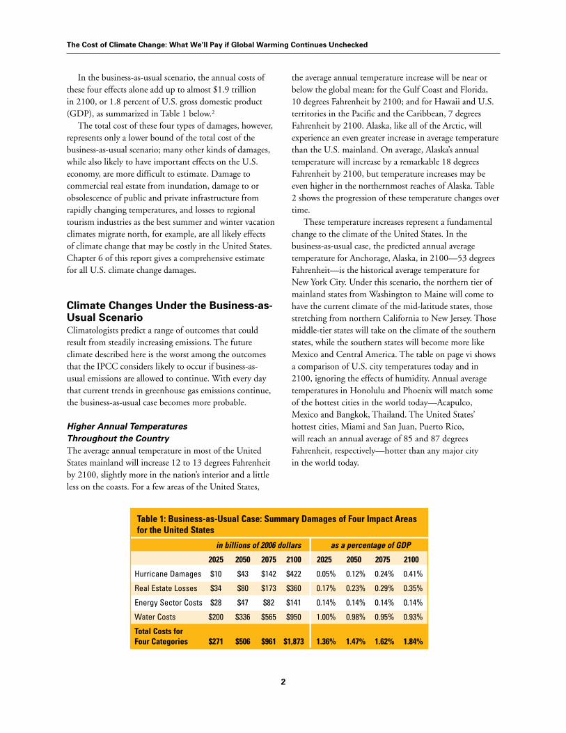
In the business-as-usual scenario, the annual costs of these four effects alone add up to almost $1.9 trillion in 2100, or 1.8 percent of U.S. gross domestic product (GDP), as summarized in Table 1 below.2

The total cost of these four types of damages, however, represents only a lower bound of the total cost of the business-as-usual scenario; many other kinds of damages, while also likely to have important effects on the U.S. economy, are more difficult to estimate. Damage to commercial real estate from inundation, damage to or obsolescence of public and private infrastructure from rapidly changing temperatures, and losses to regional tourism industries as the best summer and winter vacation climates migrate north, for example, are all likely effects of climate change that may be costly in the United States. Chapter 6 of this report gives a comprehensive estimate for all U.S. climate change damages.

Climate Changes Under the Business-as-Usual ScenarioClimatologists predict a range of outcomes that could result from steadily increasing emissions. The future climate described here is the worst among the outcomes that the IPCC considers likely to occur if business-as-usual emissions are allowed to continue. With every day that current trends in greenhouse gas emissions continue, the business-as-usual case becomes more probable.

Higher Annual Temperatures Throughout the Country The average annual temperature in most of the United States mainland will increase 12 to 13 degrees Fahrenheit by 2100, slightly more in the nation’s interior and a little less on the coasts. For a few areas of the United States,

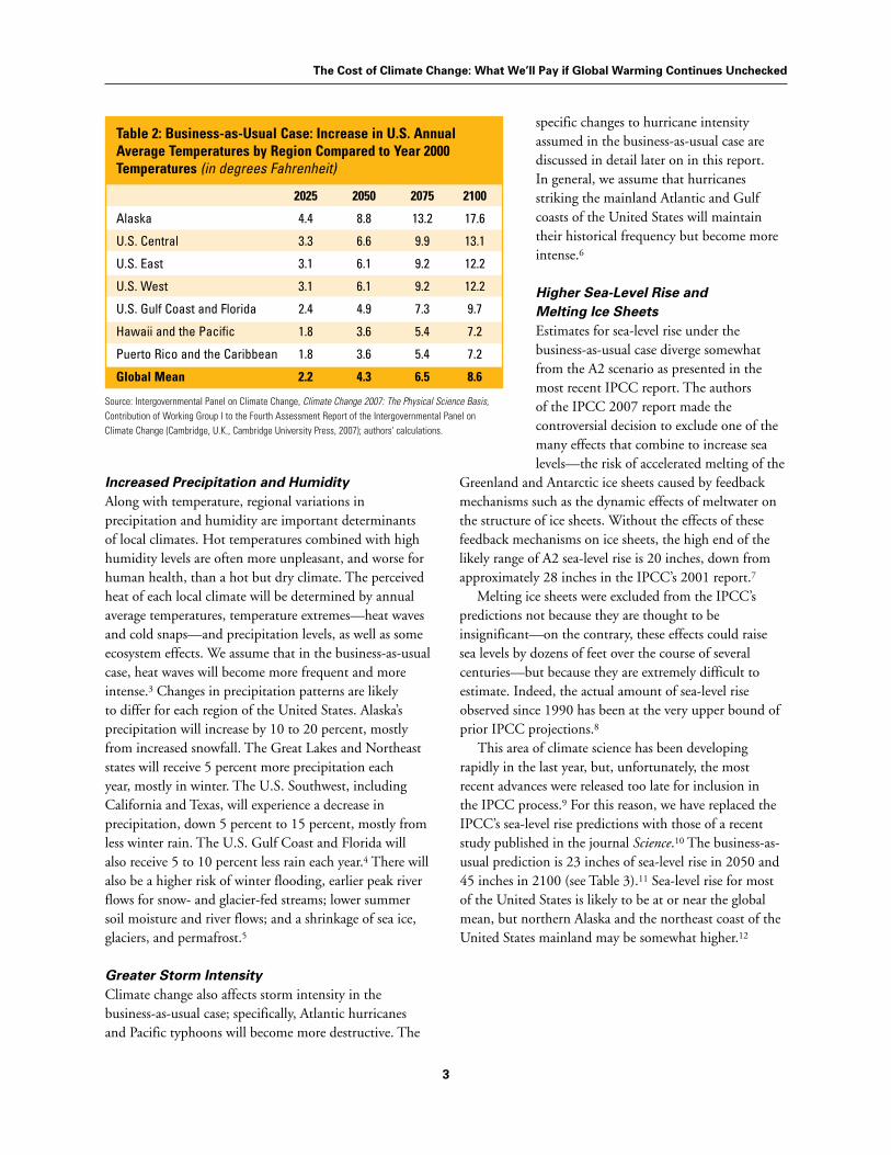
the average annual temperature increase will be near or below the global mean: for the Gulf Coast and Florida, 10 degrees Fahrenheit by 2100; and for Hawaii and U.S. territories in the Pacific and the Caribbean, 7 degrees Fahrenheit by 2100. Alaska, like all of the Arctic, will experience an even greater increase in average temperature than the U.S. mainland. On average, Alaska’s annual temperature will increase by a remarkable 18 degrees Fahrenheit by 2100, but temperature increases may be even higher in the northernmost reaches of Alaska. Table 2 shows the progression of these temperature changes over time. These temperature increases represent a fundamental change to the climate of the United States. In the business-as-usual case, the predicted annual average temperature for Anchorage, Alaska, in 2100—53 degrees Fahrenheit—is the historical average temperature for New York City. Under this scenario, the northern tier of mainland states from Washington to Maine will come to have the current climate of the mid-latitude states, those stretching from northern California to New Jersey. Those middle-tier states will take on the climate of the southern states, while the southern states will become more like Mexico and Central America. The table on page vi shows a comparison of U.S. city temperatures today and in 2100, ignoring the effects of humidity. Annual average temperatures in Honolulu and Phoenix will match some of the hottest cities in the world today—Acapulco, Mexico and Bangkok, Thailand. The United States’ hottest cities, Miami and San Juan, Puerto Rico, will reach an annual average of 85 and 87 degrees Fahrenheit, respectively—hotter than any major city in the world today.

Table 1: Business-as-Usual Case: Summary Damages of Four Impact Areas for the United States

in billions of 2006 dollars as a percentage of GDP

2025 2050 2075 2100 2025 2050 2075 2100

Hurricane Damages $10 $43 $142 $422 0.05% 0.12% 0.24% 0.41%

Real Estate Losses $34 $80 $173 $360 0.17% 0.23% 0.29% 0.35%

Energy Sector Costs $28 $47 $82 $141 0.14% 0.14% 0.14% 0.14%

Water Costs $200 $336 $565 $950 1.00% 0.98% 0.95% 0.93%

Total Costs for Four Categories $271 $506 $961 $1,873 1.36% 1.47% 1.62% 1.84%


3

Table 2: Business-as-Usual Case: Increase in U.S. Annual Average Temperatures by Region Compared to Year 2000 Temperatures (in degrees Fahrenheit)

2025 2050 2075 2100

Alaska 4.4 8.8 13.2 17.6

U.S. Central 3.3 6.6 9.9 13.1

U.S. East 3.1 6.1 9.2 12.2

U.S. West 3.1 6.1 9.2 12.2

U.S. Gulf Coast and Florida 2.4 4.9 7.3 9.7

Hawaii and the Pacific 1.8 3.6 5.4 7.2

Puerto Rico and the Caribbean 1.8 3.6 5.4 7.2

Global Mean 2.2 4.3 6.5 8.6

Increased Precipitation and Humidity Along with temperature, regional variations in precipitation and humidity are important determinants of local climates. Hot temperatures combined with high humidity levels are often more unpleasant, and worse for human health, than a hot but dry climate. The perceived heat of each local climate will be determined by annual average temperatures, temperature extremes—heat waves and cold snaps—and precipitation levels, as well as some ecosystem effects. We assume that in the business-as-usual case, heat waves will become more frequent and more intense.3 Changes in precipitation patterns are likely to differ for each region of the United States. Alaska’s precipitation will increase by 10 to 20 percent, mostly from increased snowfall. The Great Lakes and Northeast states will receive 5 percent more precipitation each year, mostly in winter. The U.S. Southwest, including California and Texas, will experience a decrease in precipitation, down 5 percent to 15 percent, mostly from less winter rain. The U.S. Gulf Coast and Florida will also receive 5 to 10 percent less rain each year.4 There will also be a higher risk of winter flooding, earlier peak river flows for snow- and glacier-fed streams; lower summer soil moisture and river flows; and a shrinkage of sea ice, glaciers, and permafrost.5

Greater Storm Intensity Climate change also affects storm intensity in the business-as-usual case; specifically, Atlantic hurricanes and Pacific typhoons will become more destructive. The

specific changes to hurricane intensity assumed in the business-as-usual case are discussed in detail later on in this report. In general, we assume that hurricanes striking the mainland Atlantic and Gulf coasts of the United States will maintain their historical frequency but become more intense.6

Higher Sea-Level Rise and Melting Ice SheetsEstimates for sea-level rise under the business-as-usual case diverge somewhat from the A2 scenario as presented in the most recent IPCC report. The authors of the IPCC 2007 report made the controversial decision to exclude one of the many effects that combine to increase sea levels—the risk of accelerated melting of the

Greenland and Antarctic ice sheets caused by feedback mechanisms such as the dynamic effects of meltwater on the structure of ice sheets. Without the effects of these feedback mechanisms on ice sheets, the high end of the likely range of A2 sea-level rise is 20 inches, down from approximately 28 inches in the IPCC’s 2001 report.7

Melting ice sheets were excluded from the IPCC’s predictions not because they are thought to be insignificant—on the contrary, these effects could raise sea levels by dozens of feet over the course of several centuries—but because they are extremely difficult to estimate. Indeed, the actual amount of sea-level rise observed since 1990 has been at the very upper bound of prior IPCC projections.8

This area of climate science has been developing rapidly in the last year, but, unfortunately, the most recent advances were released too late for inclusion in the IPCC process.9 For this reason, we have replaced the IPCC’s sea-level rise predictions with those of a recent study published in the journal Science.10 The business-as-usual prediction is 23 inches of sea-level rise in 2050 and 45 inches in 2100 (see Table 3).11 Sea-level rise for most of the United States is likely to be at or near the global mean, but northern Alaska and the northeast coast of the United States mainland may be somewhat higher.12

Source: Intergovernmental Panel on Climate Change, Climate Change 2007: The Physical Science Basis, Contribution of Working Group I to the Fourth Assessment Report of the Intergovernmental Panel on Climate Change (Cambridge, U.K., Cambridge University Press, 2007); authors' calculations.


4

Calculating the Cost of Climate Change in the Business-as-Usual ScenarioProjecting economic impacts almost a century into the future is of course surrounded with uncertainty. Any complete projection, however, would include substantial effects due to the growth of the U.S. population and economy. With a bigger, richer population, there will be more demand for energy and water—and, quite likely, more coastal property at risk from hurricanes.

In order to isolate the effects of climate change, we compare our climate forecast for business as usual with an unrealistic scenario that projects the same economic and population growth with no climate change at all, holding today’s conditions constant. The costs described here are the differences between the business-as-usual and the no climate change scenarios; that is, they are the effects of the business-as-usual climate changes alone, and not the effects of population and economic growth.13

Table 3: Business-as-Usual Scenario: Increase in U.S. Average Sea-Level Rise Compared to Year 2000 Elevation (in Inches)

2025 2050 2075 2100 Sea-Level Rise - business-as- usual prediction 11.3 22.6 34.0 45.3

Source: Intergovernmental Panel on Climate Change, Climate Change 2007: The Physical Science Basis, Contribution of Working Group I to the Fourth Assessment Report of the Intergovernmental Panel on Climate Change (Cambridge, U.K., Cambridge University Press, 2007); authors‘ calculations.


5

While climate change is popularly associated with more frequent and more intense hurricanes, within the scientific community there are two main schools of thought on this subject. One group emphasizes the role of warm sea-surface temperatures in the formation of hurricanes and points to observations of stronger storms over the last few decades as evidence that climate change is intensifying hurricanes. The other group emphasizes the many interacting factors responsible for hurricane formation and strength, saying that warm sea-surface temperatures alone do not create hurricanes.2

The line of reasoning connecting global warming with hurricanes is straightforward; since hurricanes need a sea-surface temperature of at least 79 degrees Fahrenheit to form, an increase of sea-surface temperatures above this

CHAPTER 2 More Intense Hurricanes Cause Financial Damage

Impact #1: more Intense hurrIcanes

Predicted Damage: $422 billion per year by 2100Areas Most at Risk: Atlantic and Gulf coasts

In the business-as-usual scenario, hurricane intensity will increase, with more

Category 4 and 5 hurricanes occurring as sea-surface temperatures rise. Greater

damages from more intense storms would come on top of the more severe storm

surges that will result from higher sea levels.1 Annual damages caused by increased

intensity of U.S. hurricanes will reach $422 billion in 2100, or 0.41 percent of

GDP, over and above the annual damages that would be expected if current climate

conditions remained unchanged.

threshold should result in more frequent and more intense hurricanes.3 The latest IPCC report concludes that increasing intensity of hurricanes is “likely” as sea-surface temperatures increase.4

A much greater consensus exists among climatologists regarding other aspects of future hurricane impacts. Even if climate change were to have no effect on storm intensity, hurricane damages are very likely to increase over time from two causes. First, increasing coastal development will lead to higher levels of damage from storms, both in economic and social terms. Second, higher sea levels, coastal erosion, and damage of natural shoreline protection such as beaches and wetlands will allow storm surges to reach farther inland, affecting areas that were previously relatively well protected.5


6

Table 4: Business-as-Usual Scenario: Increase in Hurricane Damages to the U.S. Mainland

2025 2050 2075 2100

Annual Damages in billions of 2006 dollars $10 $43 $142 $422 as a percentage of GSP 0.05% 0.12% 0.24% 0.41%

Annual Deaths 74 228 437 756

Hurricane Damage ProjectionsIn our business-as-usual case, the total number of tropical storms stays the same as today, but storm intensity—and therefore the number of major hurricanes—increases. In order to calculate the costs of U.S. mainland hurricanes over the next 100 years for each scenario, we took into account coastal development and higher population levels, sea-level rise as it impacts on storm surges, and greater storm intensity.

We used historical data to estimate the likely number of hurricanes, and the damages per hurricane, in an average year. If there is no change in the frequency or intensity of hurricanes, the expected impact from U.S. hurricanes in an average year is $12.4 billion (in 2006 dollars) and 121 deaths (at the 2006 population level).6

We consider three factors that may increase damages and deaths resulting from future hurricanes; each of these three factors is independent of the other two:

Coastal development and population growth—the more property and people that are in the path of a hurricane, the higher the damages and deaths.7

Sea-level rise—even with the intensity of storms remaining stable, the same hurricane results in greater damages and deaths from storm surges, flooding, and erosion.8 Hurricane intensity—in the business-as-usual case, we assume that the strength of storms increases as surface temperatures rise.9, 10

Combining these effects together, hurricane damages due to business as usual for the year 2100 would cause a projected $422 billion of damages—0.41 percent of GDP—and 756 deaths above the level that would result if today’s climate conditions remained unchanged (see Table 4).

Source: Authors’ calculations.


7

To estimate the value of real estate losses from sea-level rise, we have updated a detailed forecast of coastal real estate losses in the 48 states developed by the Environmental Protection Agency (EPA).1 In projecting these costs into the future we assume that annual costs will be proportional to sea-level rise and to projected GDP.

We calculate the annual loss of real estate from inundation due to the projected sea-level rise, which reaches 45 inches by 2100 in the business-as-usual case. These losses amount to $360 billion by 2100, or 0.35 percent of GDP, as shown in Table 5.

CHAPTER 3 Real Estate Losses as a Result of Sea Level Rise

Impact #2: reaL estate Losses

Predicted Damage: $360 billion by 2100Areas Most at Risk: Atlantic and Gulf coasts, including Florida

The effects of climate change will have severe consequences for low-lying U.S.

coastal real estate. If nothing is done to hold back rising waters, sea-level rise

will simply cause many properties in low-lying coastal areas to be inundated.

Even those properties that remain above water will be more likely to sustain storm

damage, as encroachment of the sea allows storm surges to reach inland areas that

were not previously affected. More intense hurricanes, in addition to sea-level rise, will

increase the likelihood of both flood and wind damage to properties throughout the

Atlantic and Gulf coasts.

Table 5: Business-as-Usual Scenario: Increase in U.S. Real Estate at Risk From Sea-Level Rise

2025 2050 2075 2100

Annual Increase in Value at Risk in billions of 2006 dollars $34 $80 $173 $360 as percent of GDP 0.17% 0.23% 0.29% 0.35%

Source: Titus, J.G., et al. (1991), Greenhouse Effect and Sea-Level Rise: The Cost of Holding Back the Sea, Coastal Management 19: 171-204; authors' calculations.


8

The High Cost of Adapting to Sea-Level RiseNo one expects coastal property owners to wait passively for these damages to occur; those who can afford to protect their properties will undoubtedly do so. But all the available methods for protection against sea-level rise are problematic and expensive. It is difficult to imagine any of them being used on a large enough scale to shelter all low-lying U.S. coastal lands that are at risk under the business-as-usual case.

Elevating homes and other structures is one way to reduce the risk of flooding, if not hurricane-induced wind damage. A Federal Emergency Management Agency (FEMA) estimate of the cost of elevating a frame-construction house on a slab-on-grade foundation by two feet is $58 per square foot, with an added cost of $0.93 per square foot for each additional foot of elevation.3 This means that it would cost $58,000 to elevate a house with a 1,000-square-foot footprint by two feet. It is not clear whether building elevation is applicable to multistory structures; at the least, it is sure to be more expensive and difficult.

Another strategy for protecting real estate from climate change is to build seawalls to hold back rising waters. There are a number of ecological costs associated with building walls to hold back the sea, including accelerated beach erosion; disruption of nesting and breeding grounds for important species, such as sea turtles; and prevention of the migration of displaced wetland species.5 In order to prevent flooding in developed areas, some parts of the coast would require the installation of new seawalls. Estimates for building or retrofitting seawalls range from $2 million to $20 million per linear mile.6

While adaptation, including measures to protect the most valuable real estate, will undoubtedly reduce sea-level rise damages below the amounts shown in Table 5, protection measures are expensive, and there is no single, believable technology or strategy for protecting vulnerable areas throughout the country. The high cost of adapting to sea-level rise underscores the need to act early to prevent the worst impacts of global warming.

Case Study: The Economic Effect of Sea-Level Rise in Florida

Florida is at particular risk for damages caused by a rise in sea level as a result of global warming. In the business-as-usual scenario, the annual increase in

Florida’s residential property at risk from sea-level rise reaches $66 billion by 2100, or nearly 20 percent of total U.S. damages.2

Sea-level rise will affect more than just residential property. In Florida, 9 percent of the state is vulnerable to 27 inches of sea-level rise, which would be reached soon after 2060 in the business-as-usual case. Some 1.5 million people currently live in the affected region. In addition to residential properties, worth $130 billion, Florida’s 27-inch vulnerable zone includes:

334 public schools;82 low-income housing complexes;68 hospitals;37 nursing homes;171 assisted living facilities;1,025 churches, synagogues, and mosques; 341 hazardous materials sites, including 5 superfund sites;2 nuclear reactors;3 prisons; 74 airports;115 solid waste disposal sites;140 water treatment facilities;247 gas stations277 shopping centers; 1,362 hotels, motels, and inns; and 19,684 historic structures.

Similar facilities will be at risk in other states with intensive coastal development as sea levels rise in the business-as-usual case.


9

Although we include estimates for direct use of oil and gas, our primary focus is on the electricity sector. Electricity in the United States is provided by nearly 17,000 generators with the ability to supply more than 1,000 gigawatts.1 Currently, nearly half of U.S. electrical power is derived from coal, while natural gas and nuclear each provide one-fifth of the total. Hydroelectric dams, other renewables—such as wind and solar-thermal—and oil provide the remaining power.2

As shown in Figure 1, power plants are distributed across the country. Many coal power plants are clustered along major Midwest and Southeast rivers, including the Ohio, Mississippi, and Chattahoochee. Natural gas–powered plants are located in the South along gas distribution lines and in the Northeast and California near urban areas. Nuclear plants are clustered along the eastern seaboard, around the Tennessee Valley, and along

CHAPTER 4 Costly Changes to the Energy Sector

Impact #3: chanGes to the enerGY sector

Predicted Damage: $141 billion by 2100Areas Most at Risk: Southwest, Southeast

Global warming will affect both the demand for and the supply of energy:

Hotter temperatures will mean more air-conditioning and less heating

for consumers, and more difficult and expensive operating conditions for

electric power plants. In this section, we estimate that annual U.S. energy expenditures

(excluding transportation) will be $141 billion higher in 2100—an increase equal

to 0.14 percent of GDP—in the business-as-usual case than they would be if today’s

climate conditions continued throughout the century.

the Great Lakes. Hydroelectric dams provide most of the Northwest’s electricity, and small- to medium-sized dams are found throughout the Sierras, Rockies, and Appalachian ranges. Since 1995, new additions to the U.S. energy market have come primarily from natural gas.

Higher temperatures associated with climate change will place considerable strain on the U.S. power sector as it is currently configured. Across the country, drought conditions will become more likely, whether due to greater evaporation as a result of higher temperatures or—in some areas—less rainfall, more sporadic rainfall, or the failure of snow-fed streams. Droughts clearly reduce hydroelectric output, and droughts and heat waves also put most generators at risk, adding stress to transmission and generation systems and thereby reducing efficiency and raising the cost of electricity.


10

Figure 1: U.S. Power Plants, 2006

Source: North American Electric Reliability Corporation, Electric Supply and Demand, 2007.

Note: Colors correspond to the primary fuel type, and sizes are proportional to plant capacity (output in megawatts). Only plants operational as of 2006 are included.

Water Changes Reduce Power Plant FunctioningCoal, oil, nuclear, and many natural gas power plants use steam to generate power and rely on massive amounts of water for boiling, cooling, chemical processing, and emissions scrubbing. Most plants have a minimum water requirement, and when water is in short supply, plants must reduce generation or shut down altogether.

When power plants boil water in industrial quantities to create steam, the machinery gets hot; some system for cooling is essential for safe operation. The cheapest method, when water is abundant, is so-called “open-loop” or “once-through” cooling, where water is taken from lakes, rivers, or estuaries, used once to cool the plant, and then returned to the natural environment. About 80 percent of utility power plants require water for cooling purposes, and of these, almost half use open-loop cooling.3 The “closed-loop” alternative is to build cooling towers that recirculate the water; this greatly reduces (but does not eliminate) the need for cooling water, while

making the plant more expensive to build. It is possible to retrofit plant cooling towers to reduce their water intake even more (“dry cooling”), but these retrofits are costly and can reduce the efficiency of a generator by up to 4 percent year round and nearly 25 percent in the summer during peak demand.4 Dry cooling is common only in the most arid and water-constrained regions. Yet if drought conditions persist or become increasingly common, more plants may have to implement such high-cost, low-water cooling technologies, dramatically increasing the cost of electricity production.

When lakes and rivers become too warm, plants with open-loop cooling become less efficient. Moreover, the water used to cool open-loop plants is typically warmer when it returns to the natural environment than when it is taken out, a potential cause of damage to aquatic life. The Brayton Point Power Plant on the coast of Massachusetts, for example, was found to be increasing coastal water temperatures by nearly 2 degrees, leading to rapid declines in the local winter flounder population.5


11

Case Study: Effects of Drought on Energy Production in the Southeast

In 2007, severe droughts reduced the flows in rivers and reservoirs throughout the Southeast, and high temperatures warmed what little water remained. On August 17, 2007, with temperatures soaring toward 105 degrees Fahrenheit, the Tennessee Valley Authority shut down the Browns Ferry nuclear plant in Alabama to keep river water temperatures from passing 90 degrees, a harmful threshold for downstream aquatic life.6 Even without the environmental restriction, this open-loop nuclear plant, which circulates 3 billion gallons of river water daily, cannot operate efficiently if ambient river water temperatures exceed 95 degrees Fahrenheit.7 Browns Ferry is not the only power plant vulnerable to drought in the Southeast; we estimate that more than 320 plants, or at least 85 percent of electrical generation in Alabama, Georgia, Tennessee, North

Carolina, and South Carolina, are critically dependent on river, lake, and reservoir water.8 The Chattahoochee River—the main drinking water supply for Atlanta—also supports power plants supplying more than 10,000 megawatts, more than 6 percent of the region’s generation.9 In the recent drought, the river dropped to one-fifth of its normal flow, severely inhibiting both hydroelectric generation and the fossil fuel-powered plants that rely on its flow.10 As the drought wore on, the Southern Company, a major utility in the region, petitioned the governors of Florida, Alabama, and Georgia to renegotiate interstate water rights so that sufficient water could flow to four downstream fossil-fuel plants and one nuclear facility.11

Excess energy demand due to global warming is estimated to cost $59.2 billion in the Southeast by 2100 in the business-as-usual case.

Extended droughts are increasingly jeopardizing nuclear power reliability. In France, where 5 trillion gallons of water are drawn annually to cool nuclear facilities, heat waves in 2003 caused a shutdown or reduction of output in 17 plants, forcing the nation to import electricity at more than 10 times the normal cost. In the United States, 41 nuclear plants rely on river water for cooling, the category most vulnerable to heat waves.12

The U.S. Geological Survey estimates that power plants accounted for 39 percent of all freshwater withdrawals in the United States in 2000, or 136 billion gallons per day.13 Most of this water is returned to rivers or lakes; water consumption (the amount that is not returned) by power plants is a small fraction of the withdrawals, though still measured in billions of gallons per day. The average coal-fired power plant consumes upward of 800 gallons of water per megawatt hour of electricity it produces. If we continue to build power plants using existing cooling technology, even without climate change the energy sector’s consumption of water is likely to more than double in the next quarter century, from 3.3 billion gallons per day in 2005 to 7.3 billion gallons per day in 2030.14

Droughts Reduce Hydroelectric OutputDroughts limit the amount of energy that can be generated from hydroelectric dams, which supply 6 percent to 10 percent of all U.S. power. U.S. hydroelectric generation varies with precipitation, fluctuating as much as 35 percent from year to year.17 Washington, Oregon, and Idaho, where dams account for 70, 64, and 77 percent of generation, respectively, are particularly vulnerable to drought.

The 2007 drought in the Southeast had a severe impact on hydroelectric power. As of September 2007, hydroelectric power production had fallen by 15 percent nationwide from a year earlier, and by 45 percent for the Southeastern states.16 At the time of the drought, the Federal Regulation and Oversight of Energy commission was considering reducing flows through dams in the Southeast to retain more water in reservoirs for consumption.17

Heat Waves Stress Electricity Transmission and Generation Systems Heat waves dramatically increase the cost of producing electricity and, therefore, the price to customers. During


12

periods of normal or low demand, the least expensive generators are run. During peak demand, increasingly expensive generators are brought online. During a heat wave, when demand for air-conditioning and refrigeration spikes, operators are forced to bring extremely expensive and often quite dirty plants (such as diesel engines) online to meet demand. At these times, the cost of electricity can be more expensive than during normal operations. In dire circumstances, even with all existing power plants in use, there still may not be enough electricity generated to meet demand, resulting in rolling blackouts that may cause health problems for households left without air conditioners or fans, and creating costs for business and industry.

Transmission lines, which transport energy from generators to customers, can become energy sinks during a heat wave. When temperatures rise, businesses and residents turn on air conditioners, increasing the flow of electricity over the power lines. As the lines serve more power, resistance in the lines increases—converting more of the energy to waste heat—and the system becomes less

efficient. During normal operation, about 8 percent to 12 percent of power is lost over high-voltage transmission lines and local distribution lines; during heat waves, transmission losses can add up to nearly a third of all the electricity generated.

The increased resistance in the lines also causes them to heat up and stretch, sagging between towers. Warmer ambient temperatures, as well as low wind speeds, prevent lines from cooling sufficiently, increasing their sag and the potential for a short circuit if the lines contact trees or the ground. Damaged lines force power to be shunted onto other lines, which, if near capacity, may also sag abnormally. Large-scale blackouts in the Northeast and on the West Coast have been attributed to transmission lines sagging in heat waves.18 On August 14, 2003, much of the Northeast and eastern Canada was cast into darkness in a 31-hour blackout, which exacted an economic cost estimated at $4 billion to $6 billion.19

Like transmission lines, generators that use air for cooling become significantly less efficient when ambient temperatures rise. Air-cooled gas-powered turbines can

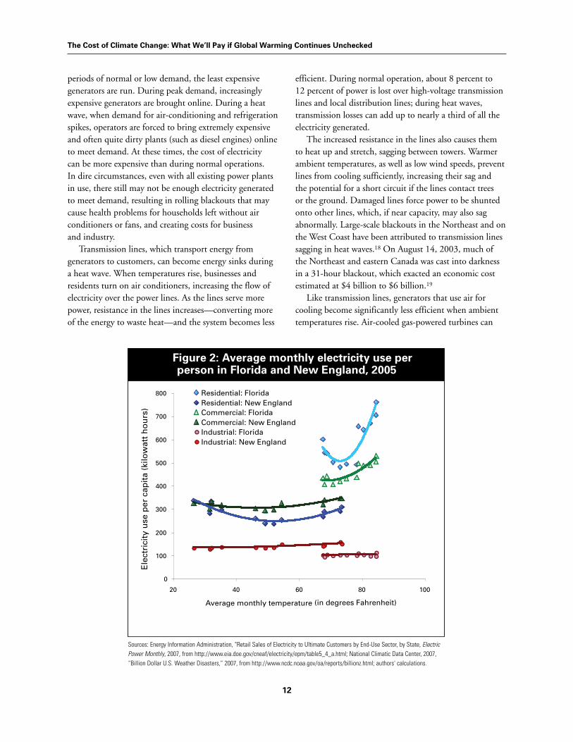
Figure 2: Average monthly electricity use per person in Florida and New England, 2005

0

100

200

300

400

500

600

700

800

20 40 60 80 100

Average monthly temperature

Ele

ctri

city

use

per

cap

ita

(kilo

wat

t h

ou

rs)

Residential: FloridaResidential: New EnglandCommercial: FloridaCommercial: New EnglandIndustrial: FloridaIndustrial: New England

(in degrees Fahrenheit)

Sources: Energy Information Administration, "Retail Sales of Electricity to Ultimate Customers by End-Use Sector, by State, Electric Power Monthly, 2007, from http://www.eia.doe.gov/cneaf/electricity/epm/table5_4_a.html; National Climatic Data Center, 2007, “Billion Dollar U.S. Weather Disasters,” 2007, from http://www.ncdc.noaa.gov/oa/reports/billionz.html; authors' calculations.


13

see efficiency losses of as much as 20 percent when air temperatures rise above 59 degrees Fahrenheit; therefore, they are used as little as possible during summer months.20 Ironically, these same gas turbines running at low efficiency are most likely to be needed when temperatures and air conditioning use spike.

Higher Temperatures Lead to More Energy ConsumptionIn the United States, monthly regional electricity consumption is closely related to average monthly temperatures.21 The highest demand for electricity comes when temperatures are at high or low points and electricity is needed for cooling and heating. At mild temperatures, when neither heating nor cooling is required, electricity demand is at its lowest.

Electricity demand versus temperature varies across regions, as shown in Figure 2. In Florida, residential customers are highly sensitive to both warm and cool temperatures, using significantly more energy when temperatures fall above or below 67 degrees Fahrenheit. The residential sector of New England is less temperature sensitive, and has a minimum energy use at 53 degrees Fahrenheit.22 This is partially due to the differing rates of use of air- conditioning across the country. In the Atlantic states from Maryland to Florida, 95 percent of homes have air conditioning, compared with less than 60 percent in New England. Only one-third of all air-conditioned homes in New England have central air-conditioning systems, compared with 80 percent in Florida.23 Therefore, it makes sense that energy usage is tightly coupled to warming temperatures in Florida and will become increasingly coupled in New England as temperatures rise.

On the other hand, less heating will be required as winters become warmer, particularly in northern states. More than half of households in the South use electricity to heat their homes, while in New England just 10 percent use electricity, half use heating oil, and about 40 percent use natural gas.24 Winter warming will reduce electricity use in Florida, but this will be outweighed by the increased electricity demand for air-conditioning. In New England, reductions in natural gas and fuel oil consumption are likely in winter, as is increasing demand for electricity as summers warm. We analyzed energy consumption changes that will likely occur as a result of global warming in the business-as-usual case and found that northern states will nearly break even on changes in

energy costs due to warming, while southern states will increase energy consumption dramatically, due to the rising use of air-conditioning.

Overall, we estimate that by 2100 in the business-as-usual case, climate change will increase the retail cost of electricity by $167 billion, and will lead to $31 billion more in annual purchases of air-conditioning units.

To estimate the energy costs associated with climate change, we examined the projected relationship between energy consumption and temperature in 20 regions of the United States.25 Monthly demand for residential, commercial, and industrial electricity; residential and commercial natural gas26; and residential fuel oil deliveries were tracked for 2005 and compared with average monthly temperatures in the largest metropolitan area (by population) in each region.27

In addition, we include a secondary set of costs for the purchase of new air conditioning systems, following the current national distribution of air conditioning. Although we include both the energy costs of decreases in heating and increases in cooling, the two are not symmetrical in their impacts on equipment costs: those who enjoy decreased heating requirements cannot sell part of their existing furnaces (at best, there will be gradual decreases in heating system costs in new structures); on the other hand, those who have an increased need for cooling will buy additional air conditioners at once.

In the business-as-usual case, increasing average temperatures drive up the costs of electricity above population and per-capita increases. Not surprisingly, electricity demand rises most rapidly in the Southeast and Southwest, as those regions experience more uncomfortably hot days. By the same token, while the Northeast and Midwest also have rising air-conditioning costs, those costs are largely offset by reduced natural gas and heating oil expenditures.

Overall, we estimate that by 2100 in the business-as-usual case, climate change will increase the retail cost of electricity by $167 billion, and will lead to $31 billion more in annual purchases of air-conditioning units.

At the same time, warmer conditions will lead to a reduction of $57 billion in natural gas and heating oil expenditures. Overall costs in the energy sector in the business-as-usual case add up to $141 billion more in 2100 due to climate change alone, or 0.14 percent of projected U.S. GDP in 2100.


14

The “Lowball” Average: Designing the Energy Sector for Extremes

Our estimates are based on averages: average temperature changes, average monthly temperatures, and aggregate monthly energy use in large regions. In reality, however, the capacity of the energy sector must be designed for the extremes: Air-conditioning is used most heavily on the hottest of days, while heating requirements peak on the coldest days of the year. Since energy costs climb rapidly when demand is high and the system is stretched, many costs will be defined by extremes as well as average behavior.

One of the most severe climate strains on the electricity sector will be intensifying heat waves. During a heat wave, local grids can be pushed to the limit of their capacity just by virtue of many air-conditioning units operating simultaneously. Heat waves and droughts (both expected to become more common conditions, according to the IPCC) will push the costs of electricity during times of shortage well beyond the costs included in our model. Therefore, a full cost accounting must consider not only the marginal cost of gradually increasing average temperatures, but electricity requirements on the hottest of days, when an overstressed energy sector could be fatal. Similarly, savings in natural gas and fuel oil in the north could be quickly erased by extended cold snaps even as the average temperature rises. In addition, this model cannot quantify the substantial costs of reduced production at numerous hydroelectric facilities, nuclear facilities that are not able to draw enough cooling water to operate, conflicts between water-intensive power suppliers, the costs of retrofitting numerous plants for warmer conditions, and reduced power flow from decreasingly efficient natural gas plants.

Table 6: Business-as-Usual Scenario: Increases in Energy Costs, 2100 Compared With 2005 Levels

in billions of 2006 dollars West, Total Southwest South Southeast Northeast Midwest Northwest in 2100

Electricity $62.3 $20.4 $58.9 $10.5 $10.2 $4.7 $166.9

Heating Oil $0.0 $0.0 -$0.2 -$3.1 $0.0 $0.0 -$3.4

Natural Gas -$9.5 -$4.0 -$6.7 -$10.7 -$16.8 -$5.9 -$53.7

AC Units $4.0 $2.5 $7.3 $6.2 $7.5 $3.5 $30.9

Total $56.8 $18.9 $59.2 $2.8 $0.9 $2.2 $140.7

Source: Authors’ calculations.

Note: AC Units refers to the purchase of additional air-conditioning units. Totals may not add up exactly due to rounding.


15

Water Trends Across the United StatesPrecipitation in the United States increased, on average, by 5 percent to 10 percent during the 20th century, but this increase was far from being evenly distributed in time or space. Most of the increase occurred in the form of even more precipitation on the days with the heaviest rain or snowfalls of the year.2 Geographically, stream flows have been increasing in the eastern part of the country, but decreasing in the West. As temperatures have begun to rise, an increasing percentage of precipitation in the Rockies and other western mountains has been falling as rain rather than snow.3

CHAPTER 5 Water and Agriculture Hit Hard by Global Warming

Impact #4: proBLems For Water anD aGrIcuLture

Predicted Damage: $950 billion by 2100Areas Most at Risk: American West

In many parts of the country, the most important impact of climate change during

the 21st century will be its effect on the supply of water. Recent droughts in the

Southeast and in the West have underscored our dependence on the fluctuating

natural supply of freshwater. With five out of every six gallons of water used in the

United States consumed by agriculture, any changes in water supply will quickly

ripple through the nation’s farms as well.1 Surprisingly, studies from the 1990s often

projected that the early stages of warming would boost crop yields. This section

surveys the effects of climate change on water supply and agriculture, finding that the

costs of business as usual for water supply could reach almost $1 trillion per year by

2100, while the anticipated gains in crop yields may be small, and would in any case

vanish by mid-century.

While there have been only small changes in average conditions, wide year-to-year variability in precipitation and stream flows has led to both droughts and floods, with major economic consequences. The 1988 drought and heat wave in the central and eastern United States caused $69 billion of damages (in 2006 dollars) and may have caused thousands of deaths. One reason for the large losses was that the water level in the Mississippi River fell too low for barge traffic, requiring expensive alternative shipping of bulk commodities. In recent years, the 1988 drought is second only to Hurricane Katrina in the costs of a single weather disaster (NCDC 2007).4 Growing


16

demand has placed increasing stresses on the available supplies of water, especially—but not exclusively—in the driest parts of the country. 4 In the West, the spread of population, industry,

and irrigated agriculture has consumed the region’s limited sources of water; cities are already beginning to buy water rights from farmers, having nowhere else to turn.5 The huge Ogallala Aquifer—a primary source of water for irrigation and other uses in South Dakota, Nebraska, Wyoming, Colorado, Kansas, Oklahoma, New Mexico, and Texas—is being depleted, with withdrawals far in excess of the natural recharge rate.6

4 In the Southwest, battles over allocation and use of the Colorado River’s water have raged for decades.7

4 In the Northwest, wetter states have seen conflicts between farmers who are dependent on diversion of water for irrigation, and Native Americans and others who want to maintain the river flows needed for important fish species such as salmon.

4 In Florida, one of the states with the highest annual rainfall, the rapid pace of residential and tourist development and the continuing role of irrigated winter agriculture have led to water shortages, which have been amplified by the current drought.8

Rising Demand for WaterWater use per capita is no longer rising, as more and more regions of the country have turned to conservation efforts. But new supplies of water are required to meet the needs of a growing population and to replace unsustainable current patterns of water use. Thus even if there were no large changes in precipitation, much of the country would face expensive problems of water supply in the course of this century. Responses are likely to include intensified water conservation measures, improved treatment and recycling of wastewater, construction and upgrading of cooling towers to reduce power plant water needs, and reduction in the extent of irrigated agriculture.

A study done as part of the national assessment of climate impacts, conducted by the U.S. Global Change Research Program (USGCRP) in 1999-2000, estimated the costs of future changes in water supply for the 48 coterminous states, with and without climate change.9 In the absence of climate change, i.e., assuming that the climate conditions and water availability of 1995 would continue unchanged for the next century, an annual water cost increase (in 2006 dollars) of $50 billion by 2095

was projected. The study calculated water availability separately for 18 regions of the country, projecting a moderate decline in irrigated acreage in the West and an increase in some parts of the Southeast and Midwest. Since the lowest-value irrigated crops would be retired first, the overall impact on agriculture was small.

Forecasting ScarcityIn the business-as-usual future, problems of water supply will become more serious, as much hotter—and in many areas drier—conditions will increase demand. The average temperature increase of 12 to 13 degrees Fahrenheit across most of the country, and the decrease in precipitation across the South and Southwest, as described above, will lead to water scarcity and increased costs in much of the country.

Projecting future water costs is a challenging task, both because the United States consists of many separate watersheds with differing local conditions and because the major climate models are only beginning to produce regional forecasts for areas as small as a river basin or watershed. A recent literature review of research on water and climate change in California commented on the near-total absence of cost projections.10 The estimate appears to be the best available national calculation, despite limitations that probably led the authors to underestimate the true costs.

The national assessment by the USGCRP used forecasts to 2100 of conditions under the IPCC’s IS92a scenario, a midrange IPCC scenario that involves slower emissions growth and climate change than our business-as-usual case. Two general circulation models were used to project regional conditions under that scenario; these may have been the best available projections in 1999, but they are quite different from the current state of the art.11 One of the models (the Hadley 2 model) was at that time estimating that climate change would increase precipitation and decrease water supply problems across most of the United States. This seems radically at odds with today’s projections of growing water scarcity in many regions.

The other model included in the national assessment—the Canadian Global Climate Model—projected drier conditions for much of the United States, seemingly closer to current forecasts of water supply constraints. The rest of this discussion relies exclusively on the Canadian model forecasts. Yet that model, as of 1999, was projecting that the Northeast would become drier


17

while California would become wetter—the reverse of the latest IPCC estimates (see the detailed description of the business-as-usual scenario in Chapter 1).

USGCRP estimated the costs for an “environmental management” scenario, assuming that each of the 18 regions of the country needed to supply the lower of the desired amount of water, or the amount that would have been available in the absence of climate change. The cost of that scenario was $612 billion per year (in 2006 dollars) by 2095.12 Most of the nationwide cost was for new water supplies in the Southeast, including increased use of recycled wastewater and desalination. The climate scenario used for the analysis projected a national average temperature increase of 8.5 degrees Fahrenheit by 2100, or about two-thirds of the increase under our business-as-usual scenario. Assuming the costs incurred for water supply are proportional to temperature increases, the USGCRP methodology would imply a cost of $950 billion per year by the end of the century as a result of business-as-usual climate change, compared with the costs that would occur without climate change.13

Although these costs are large, they still omit an important impact of climate change on water supplies. The calculations described here are all based on annual supply and demand for water, ignoring the problems of seasonal fluctuations. In many parts of the West, the mountain snowpack that builds up every winter is a natural reservoir, gradually melting and providing a major source of water throughout the spring and summer seasons of peak water demand. With warming temperatures and the shift toward less snow and more rain, areas that depend on snowpack will receive more of the year’s water supply in the winter months. Therefore, even if the total volume of precipitation is unchanged, less of the flow will occur in the seasons when it is most needed. In order to use the increased winter stream flow later in the year, expensive (and perhaps environmentally damaging) new dams and reservoirs will have to be built. Such seasonal effects and costs are omitted from the calculations in this section.

Moreover, there has been no attempt to include the costs of precipitation extremes, such as floods or droughts, in the costs developed here (aside from the hurricane estimates discussed above). The costs of extreme events are episodically quite severe, as suggested by the 1988 drought, but also hard to project on an annual basis.Despite these limitations, we take the USGCRP estimate, scaled up to the appropriate temperature increase, to be the best available national cost estimate

for the business-as-usual scenario. There is a clear need for additional research to update and improve on this cost figure.

Water Supply and the Agriculture IndustryClimate change threatens to damage American agriculture, with drier conditions in many areas and greater variability and extreme events everywhere. Agriculture is the nation’s leading use of water, and the U.S. agricultural sector is shaped by active water management: Nearly half of the value of all crops comes from the 16 percent of U.S. farm acreage that is irrigated.14 Especially in the West, any major shortfall of water will be translated into a decline in food production.

As one of the economic activities most directly exposed to the changing climate, agriculture has been a focal point of research on climate impacts, with frequent claims of climate benefits, especially in temperate regions like much of the United States.

The initial stages of climate change appear to be beneficial to farmers in the northern states. In the colder parts of the country, warmer average temperatures mean longer growing seasons. Moreover, plants grow by absorbing carbon dioxide from the atmosphere; so the rising level of carbon dioxide, which is harmful in other respects, could act as a fertilizer and increase yields. A few plant species, notably corn, sorghum, and sugarcane, are already so efficient in absorbing carbon dioxide that they would not benefit from more, but for all other major crops, more carbon could allow more growth. Early studies of climate costs and benefits estimated substantial gains to agriculture from the rise in temperatures and carbon dioxide levels.15 As recently as 2001, in the development of the USGCRP’s national assessment, the net impact of climate change on U.S. agriculture was projected to be positive throughout the 21st century.16

Recent research, however, has cast doubts on any agricultural benefits of climate change. More realistic,

Table 7: Business-as-Usual Scenario: Increases in U.S. Water Costs Compared With 2005 Levels

2025 2050 2075 2100

Annual Increase in Costs in billions of 2006 dollars $200 $336 $565 $950 as percent of GDP 1.00% 0.98% 0.95% 0.93%

Sources: Frederick, K. D., and G. E. Schwartz, "Socioeconomic Impacts of Climate Variability and Change on U.S. Water Resources," Resources for the Future, 2000; authors' calculations.


18

outdoor studies exposing plants to elevated levels of carbon dioxide have not always confirmed the optimistic results of earlier greenhouse experiments.17 In addition, the combustion of fossil fuels, which increases carbon dioxide levels, will at the same time create more tropospheric (informally, ground-level) ozone—and ozone interferes with plant growth. A study that examined the agricultural effects of increases in both carbon dioxide and ozone found that in some scenarios, ozone damages outweighed all climate and carbon dioxide benefits.18 In this study and others, the magnitude of the effect depends on the speed and accuracy of farmers’ response to changing conditions: Do they correctly perceive the change and adjust crop choices, seed varieties, planting times, and other farm practices to the new conditions? In view of the large year-to-year variation in climate conditions, it seems unrealistic to expect rapid, accurate adaptation. The climate “signal” to which farmers need to adapt is difficult to interpret, and errors in adaptation could eliminate any potential benefits from warming.

The passage of time will also eliminate any climate benefits to agriculture. Once the temperature increase reaches 6 degrees Fahrenheit, crop yields everywhere will be lowered by climate change.19 Under the business-as-usual scenario, that temperature threshold is reached by mid-century. Even before that point, warmer conditions may allow tropical pests and diseases to move farther north, reducing farm yields. And the increasing variability of temperature and precipitation that will accompany climate change will be harmful to most or all crops.20

One recent study examined the relationship between the market value of U.S. farmland and its current climate; the value of the land reflects the value of what it can produce.21 For the area east of the 100th meridian, where irrigation is rare, the value of an acre of farmland is closely linked to temperature and precipitation.22 Land value is maximized—meaning that conditions for agricultural productivity are ideal—with temperatures during the growing season, April through September, close to the late-20th-century average, and rainfall during the growing season of 31 inches per year, well above the historical average of 23 inches.23 If this relationship remained unchanged, then becoming warmer would increase land values only in areas that are colder than average; becoming drier would decrease land values almost everywhere.

For the years 2070 to 2099, the study projected that the average value of farmland would fall by 62 percent under the IPCC’s A2 scenario, the basis for our business-as-usual case. The climate variable most strongly

connected to the decline in value was the greater number of days above 93 degrees Fahrenheit, a temperature that is bad for virtually all crops. The same researchers also studied the value of farmland in California, finding that the most important factor there was the amount of water used for irrigation; temperature and precipitation were much less important in California than in eastern and midwestern agriculture.24

It is difficult to project a monetary impact of climate change on agriculture; if food becomes less abundant, prices will rise, partially or wholly offsetting farmers’ losses from decreased yields. This is also an area where assumptions about adaptation to changing climatic conditions are of great importance: The more rapid and skillful the adaptation, the smaller the losses will be. It appears likely, however, that under the business-as-usual scenario, the first half of this century will see either little change or a small climate-related increase in yields from non-irrigated agriculture; irrigated areas will be able to match this performance if sufficient water is available. By the second half of the century, as temperature increases move beyond 6 degrees Fahrenheit, yields will drop everywhere.

In a broader global perspective, the United States, for all its problems, will be one of the fortunate countries. Tropical agriculture will suffer declining yields at once, as many crops are already near the top of their sustainable temperature ranges. At the same time, the world’s population will grow from an estimated 6.6 billion today to 9 billion or more by mid-century—with a large portion of the growth occurring in tropical countries. The growing, or at least non-declining, crop yields in temperate agriculture over the next few decades will be a valuable, scarce global resource. The major producing regions of temperate agriculture—the United States, Canada, northern China, Russia, and northern Europe, along with Argentina, Chile, Australia, New Zealand, and South Africa—will have an expanded share of the world’s capacity to grow food, while populations are increasing fastest in tropical countries where crop yields will be falling. The challenge of agriculture in the years ahead will be to develop economic and political mechanisms that allow us to use our farm resources to feed the hungry worldwide. At the same time, while we may fare better than other nations, climate change threatens to damage American agriculture, with drier conditions in many areas and greater variability and extreme events everywhere.


19

This chapter discusses the results of the PAGE model for the United States, both in the form used in the Stern Review and with several new analyses and calculations developed specifically for this report.2 Our newly revised PAGE model results project that total U.S. damages will amount to as much as 3.6 percent of GDP in 2100.3 This comprehensive estimate includes several categories of damages that are not included in our detailed case studies; for the category of damages that includes the four impacts we studied in detail, even the new PAGE results appear

to be too low. That is, a further revision to be consistent with our case studies would imply climate damages even greater than 3.6 percent of GDP by 2100.

U.S. Damages in the Stern Review The PAGE model used by the Stern Review estimates the damages caused by climate change for eight regions of the world, including the United States, through 2200. While the case studies presented in earlier chapters provide a

CHAPTER 6 Modeling U.S. Climate Impacts: Beyond the Stern Review

Economic analysis of climate change took a major step forward with the

publication of the Stern Review in 2006, sponsored by the British government

and directed by prominent British economist Nicholas Stern. The Stern

Review offered a thoughtful synthesis of the state of climate science and presented

the results of an innovative economic model of climate damages. The PAGE model,1

used by Stern, estimates that climate damages from emissions through 2200 could

be equivalent to 5 to 20 percent of world output each year on an ongoing basis.

However, for the United States alone, the PAGE model as used by Stern projects much

smaller impacts: a 1 percent loss of U.S. GDP in 2100 for a scenario similar to our

business-as-usual case. This is a serious underestimate in comparison with the loss of

1.8 percent of U.S. GDP, from just a subset of four climate impacts, documented in

this report. On the other hand, it is much less of an underestimate than many of the

economic predictions that came before it.


20

“detailed” accounting of costs—building upward from historical data on climate impacts—the PAGE method takes a “comprehensive” approach: It begins with a general rule about how climate affects the country as a whole and then applies that rule to business-as-usual climate forecasts. Three categories of climate impacts are included in PAGE: 4 Economic impacts on sectors such as agriculture and

energy use, which have market prices and are directly included in GDP;

4 Non-economic impacts, such as changes in human health, effects on wilderness areas and endangered

species, etc., which are not directly included in GDP; and

4 Discontinuity impacts, which are increased risks of catastrophic events such as the melting of the Greenland and West Antarctic ice sheets.

The four impacts we examine in Chapters 2 through 5 are a subset of the first category; they are economic damages with market prices.

The PAGE model’s underlying demographic, economic, and emissions data are taken from the A2 scenario of the IPCC’s Third Assessment Report.7 The

Stern Report Introduces Innovations in Economic Modeling of Global Warming

There are two principal innovations in the Stern Review’s economic modeling. First, the discount rate was set at an average of 1.4 percent per year, low enough to make future impacts important in today’s decisions. At discount rates as high as 5 percent or more, favored by many other economists, the far future simply doesn’t matter much today. A discount rate of 1.4 percent means that our actions now can still affect the future climate in a meaningful way.

Stern’s choice of a 1.4 percent discount rate is based almost entirely on the assumption of ongoing economic growth, assumed to be 1.3 percent annually: If future generations are going to be somewhat richer than we are, there is correspondingly less need to worry about their welfare today. The rate of “pure time preference,” that is, the discount rate that would apply if all generations had the same per capita income, was set at only 0.1 percent per year. As Stern convincingly argued, pure time preference close to zero is required on ethical grounds—people are of equal importance regardless of when they are born—and it is essential for an economic analysis that values a sustainable future.

The second innovation is the explicit treatment of uncertainty. Many of the key parameters for an economic analysis of climate change are uncertain: For example, what is the best estimate of “climate sensitivity,” the long-run temperature increase that will result from a doubling of carbon dioxide concentrations? How fast will economic damages increase as temperatures rise? What temperature is likely to trigger a catastrophe such as the complete collapse and melting of the Greenland ice sheet? For questions such as these, most economic models use a single “best guess” based on limited data. Because the data are limited, however, the answers to these questions are still subject to considerable uncertainty.

In order to reflect the effects of uncertainty, the Stern Review replaces this best guess methodology with a statistical technique called Monte Carlo analysis4. For each of the uncertain parameters, a range of possible values is established, and one of these values is picked at random whenever the model is run. The model is run many times, and the results of all the runs are averaged.

Monte Carlo analysis generally leads to larger estimates of climate damages than a model restricted to best guesses. Roughly speaking, the reason is that the climate could potentially get much worse, but only moderately better, than the “most likely” estimate. So including both best and worst cases, as well as the central estimate, makes the average outcome worse. Replacing the Monte Carlo analysis with fixed best guesses, as in most other models, would have the same bottom-line effect as doubling the discount rate.5 Indeed, the combination of a low discount rate and the Monte Carlo analysis of uncertainty is the principal reason why the Stern Review finds immediate, vigorous climate policy to be cost-effective. This conclusion is at odds with, and has been criticized by, economists who remain wedded to more traditional approaches.6

The use of Monte Carlo analysis, however, does not guarantee that uncertainty has been adequately incorporated. Indeed, plausible modifications to the Stern analysis lead to very different estimates.


21

global results of the PAGE model as reported in the Stern Review range from a 5 percent loss of GDP for economic impacts alone, up to a 20 percent loss of GDP for all three categories of economic, non-economic, and discontinuity impacts combined, using high (more damaging) assumptions about some remaining controversies in climate science.

Impacts as a fraction of GDP are, not surprisingly, much smaller for the United States than for the world. The worst impacts of climate change will be felt first in the hottest and poorest regions of the world, not in North America. Many parts of the United States enjoy a relatively cool climate, and the country has ample resources for adaptation to the early stages of climate change—although not always the foresight to use those resources wisely. Even compared to other rich countries, the United States is less vulnerable; for example, a much greater proportion of Europe’s population and economic activity is concentrated along the coasts, where it is vulnerable to sea-level rise and storm surges. The Stern Review assumes that low-cost adaptation eliminates 100 percent of U.S. and other developed country economic impacts for up to 3.6 degrees Fahrenheit of warming, and 90 percent of impacts at larger temperature increases. Adaptation is assumed to do much less for the other categories of impacts, reducing the non-economic impacts by only 25 percent and catastrophic damages not at all.

Figure 3 shows the Stern Review’s mean estimate of the three categories of impacts on the United States. (In the

graph, the vertical distance between the lines represents the size of the impacts.) Stern’s strong assumption about adaptation makes the economic impacts unimportant. The other impacts grow rapidly in the later years, with the combined total of all three categories amounting to only 0.1 percent of GDP in 2050, but rising to 0.4 percent by 2100 and 1.8 percent by 2200. The Stern Review reports PAGE model results through 2200; as the graph illustrates, the expected impacts become much larger in the next century.

Global impacts are about five times that large, roughly 10 percent of output in 2200. The United States emits about 20 percent of global emissions from now to 2200, but suffers only about 5 percent of global impacts.8

The results shown in Figure 3 are for the most likely impact, or the 50th percentile result. The results that would be most comparable to the business-as-usual case presented in this report, however, are at the high end of the likely range, or the 83rd percentile. The most pessimistic of the Stern Review’s likely business-as-usual results (or the 83rd percentile) for the United States was 0.2 percent of the U.S. GDP in 2050 and 1 percent in 2100 for economic, noneconomic, and catastrophic damages combined. (The remainder of this chapter is based on 83rd percentile results from the PAGE model.)

economic

discontinuity

non-economic

-2.00

-1.50

-1.00

-0.50

0.002000 2020 2040 2060 2080 2100 2120 2140 2160 2180 2200

Per

cen

t o

f G

DP

Figure 3: Mean U.S. Impacts in the Stern Review’s Baseline Scenario

Source: Hope, C., and S. Alberth, "U.S. Climate Change Impacts from the PAGE2002 Integrated Assessment Model Used in the Stern Report," Judge Business School Working Paper (University of Cambridge, 2007).


22

New Modeling Expands on Stern’s EstimatesAlthough the Stern Review represents a significant advance over conventional analyses, it is far from being the last word on the economics of climate change. In several respects, Stern appears to have chosen arbitrary, overly cautious assumptions that tend to lower the estimate of climate damages. Our revised application of the PAGE model (created for this report by the developer of the PAGE model) presents an alternative analysis that builds on the Stern Review to more accurately capture the true costs of climate change.

Eliminating Assumptions About Adaptation The Stern Review damage estimates, particularly for the United States and other high-income countries, are understated by the treatment of adaptation: Stern never reports his actual estimate of total damages, but only the damages that would remain after an extremely extensive but low-cost adaptation effort. As noted above, Stern assumes that adaptation in developed countries eliminates all economic damages from the first 3.6 degrees Fahrenheit of warming, 90 percent of economic damages above 3.6 degrees Fahrenheit, and 25 percent of all noncatastrophic health and environmental damages. In

Inside the Black Box of Economic Models

Chapters 1 through 5 show that just four of the major impacts of global warming will cause damages projected to reach 1.8 percent of U.S. GDP by 2100 in the business-as-usual case. Total damages to the U.S. economy, including many other impacts, will be larger than these estimates. Based on these findings, models that have predicted small climate costs, or even net benefits, to the U.S. economy appear to have underestimated the scale of the problem.

Our analysis examines what happens inside the black box of conventional economic models, finding a pattern of arbitrary and biased assumptions—with the bias almost always in the direction of minimizing the costs of climate change.

To understand and respond to climate change, it is essential to forecast what will happen at carbon dioxide concentrations and temperature levels that are outside the range of human experience. In the realm of science there is substantial agreement, at least in broad outline, about the physical relationships that govern these predictions. Reflecting that agreement, today’s scientific models have achieved remarkably detailed forecasts of future climatic conditions, with a gradually increasing degree of consensus among models.

In the realm of economics, however, there is much less agreement about the laws and patterns that will govern future development. Numerous economic models weigh the costs of allowing climate change to continue against the costs of stopping or slowing it, and thus recommend a “best” course of action: one that, given the assumptions of a particular model, would cause the least harm. The problem lies in the choice of assumptions.

Models of climate economics do not just swallow economic data and spit out predictions of future economic conditions. Inevitably, they embody ethical and political judgments; they make assumptions about how we value the lives, livelihoods, and natural ecosystems of future generations—how contemporary human society feels about those who will inherit the future. The models also make assumptions about future patterns of economic growth and technological change, technical questions on which economists do not all agree about the answers. Thus the economic results are driven by conjectures and assumptions that do not rest on empirical evidence, and often cannot be tested against data until after the fact.

More specifically, models that summarize the monetary value of climate damages are often inconsistent with common sense about how climate change will impact society in several ways: 1) Uncertain outcomes are disregarded, even when the possible impacts are catastrophic; instead, most economic models focus on the most likely climate impact; 2) Costs to future generations are assumed to be much less important, and less valuable, than costs experienced today; 3) Dubious price tags are given to non-economic losses, like damages to human health or the environment, for which no amount of money can adequately compensate; and 4) The early stages of warming are often assumed to be beneficial, even when the evidence is scant or contradictory. Surprisingly arbitrary methods are used to determine the overall scale of damages.


23

order to better understand the Stern estimates, we re-ran the same model assuming no adaptation. This change has the result of doubling the baseline Stern estimates. Damages in the no-adaptation scenario amount to 0.4 percent of U.S. GDP in 2050 and 1.7 percent in 2100, including economic, non-economic, and catastrophic impacts.

Modeling the “no adaptation” scenario is not meant to imply that this is a likely outcome; there will undoubtedly be successful adaptation to many aspects of climate damages. It is useful as a starting point, however, to see how much damage there would be, if there were no adaptation or mitigation. That damage estimate can then be compared with the costs of adaptation and mitigation. Stern’s results are presented only as the net effect after an assumed high level of low-cost adaptation; we have no way of knowing exactly how much adaptation will eventually take place at what cost.

Moreover, the Stern assumption of low-cost, successful adaptation to virtually all economic damages seems overly optimistic in the aftermath of Hurricane Katrina. The United States certainly had the resources to protect New Orleans and other affected communities; and, paralleling Stern’s assumption, the cost of adaptation (such as bigger and better levees) would have been a small fraction of the cost of the damages caused by the storm. Yet it is not enough to have the resources for adaptation and, as in the case of Katrina, clear advance warning of potential harms. Unless we have the political will and foresight to listen to the warnings and actually build the levees, adaptation will not occur.

What percentage of the needed adaptation to climate impacts will actually occur in the future? The unfortunate lessons of the Katrina experience itself could lead to doing better next time—but the Stern assumption of 90 to 100 percent successful adaptation to non-catastrophic damages will not be achieved unless there is a substantial change in U.S. emergency preparedness and climate policy.

More Accurately Addressing High Temperature DamagesHow fast will damages increase as average temperatures rise? How soon will the world face real risks of an abrupt, catastrophic event such as the complete loss of the Greenland ice sheet (which would raise sea levels more than 20 feet and destroy most coastal communities around the world)? These are among the most important questions in forecasting future climate damages. In both cases, the PAGE model analysis in the Stern Review

makes surprisingly cautious projections, while the text of the Stern Review paints a more ominous picture of the future. Here we explore a set of three changes to the model, all addressing these uncertainties.

One change involves the shape of the damage function. PAGE, like many economic models, assumes climate damages are a function of temperature, using a simple equation:

Damages = aTN

Here, a is a constant, T is the temperature increase (usually relative to a recent base year), and N is the exponent governing how fast damages rise as the world gets hotter. If N = 1, then this equation tells us that 4 degrees is twice as bad as 2 degrees; if N = 2, 4 degrees is four times as bad as 2 degrees; if N = 3, then 4 degrees is eight times as bad as 2 degrees, etc.

PAGE treats the exponent N in this equation as one of the uncertain parameters that are allowed to vary in the Monte Carlo analysis. For the Stern Review, it had a minimum of 1, most likely value of 1.3, and maximum of 3. There is essentially no evidence bearing directly on the value of this exponent, but the “most likely” value of 1.3 seems almost timid: It implies that 4 degrees is only about 2.5 times as bad as 2 degrees. In our variation, we set the minimum at 1.5, most likely value at 2.25, and maximum at 3. This alternative keeps the exponent within the same range used in the Stern Review but weights the higher end of the range more heavily; it assumes that the exponent is most likely to be a little more than 2, the value used in many recent models.

A second change involves the temperatures that trigger catastrophic damages. PAGE assumes that a threshold temperature (again measured in degrees above a recent base year) must be reached before catastrophic events become possible; once that threshold is crossed, the probability of catastrophe gradually rises along with the temperature. Two of the uncertain (Monte Carlo) parameters in PAGE are involved here. One is the threshold temperature, with a minimum of 3.6, most likely value of 9, and maximum of 14.4 (all in degrees Fahrenheit) in the Stern analysis. Much of the discussion of potential catastrophes, such as the loss of the Greenland or West Antarctic ice sheets, has suggested that they become possible or even likely at temperatures well below the PAGE model’s “most likely” threshold of 9 degrees Fahrenheit of warming; even the narrative portions of the Stern Review make this suggestion. For this reason, the


24

baseline assumption about threshold temperatures seems too conservative. We changed the threshold temperature to a minimum of 3.6, most likely value of 5.4, and maximum of 7.2 (again in degrees Fahrenheit).

Revising Estimates of the Probability of CatastropheAnother key to this calculation is the rate at which the probability of catastrophe grows as the temperature rises past the threshold. For Stern, the probability of catastrophe increases by a minimum of 1, most likely value of 10, and maximum of 20 percentage points per degree Celsius (i.e., per 1.8 degrees Fahrenheit) above the threshold. This also seems unduly conservative, minimizing the risk of catastrophe until warming is far advanced. In our changes to the model, the probability of catastrophe grows at a minimum of 10, most likely rate of 20, and maximum of 30 percentage points per degree Celsius above the threshold.

Adding this group of changes to the no-adaptation scenario has very little effect by 2050; even with the revised assumptions, a catastrophe remains quite unlikely in the first half of the century. Beyond that point, however, the increased risk of disaster grows rapidly. The comprehensive estimate of damages from our revised version of the PAGE model reaches 0.46 percent of U.S. GDP in 2050 and 3.61 percent of GDP in 2100.

The PAGE Model and the Four Estimated ImpactsThis exploration of alternatives within the PAGE model suggests important ways in which Stern’s estimates may understate the likely impacts of climate change on the U.S. economy and has offered an alternative, noticeably higher estimate based on changing a few key assumptions. But even the best application of such models rests on many abstract assumptions, which are difficult to verify.

Our revised runs of the comprehensive PAGE model provide aggregate damage estimates that look larger than the detailed case study estimates in Chapters 2 through 5. Recall, however, that PAGE estimates combine economic damages, noneconomic impacts, and catastrophic risks. Our case study estimates of the costs of business as usual, reaching 1.8 percent of U.S. GDP by 2100, should be compared with a subset of the PAGE economic damages. In fact, in our revised PAGE runs as well as in the Stern

version, most of the PAGE damage estimates for the United States reflect the non-economic and catastrophic categories. Our case study results are considerably larger than the corresponding PAGE estimates for the economic cost category. This suggests that if the PAGE economic costs were adjusted to be comparable with the case studies, the result would be an even greater damage estimate. Even the best of the existing economic models of climate change cannot yet reflect the full extent of damages that would result from business as usual.


25

CHAPTER 7 Conclusion

Estimates of future economic damages resulting from climate change have an

important impact on policy decisions being made today. Reducing greenhouse

gas emissions and protecting ourselves from those impacts will be costly, but a

failure to act to address climate change would be even more expensive.

In this report, we have started from the bottom up to measure just a handful of potential damages from climate change to the United States: hurricanes, residential real estate, energy, and water. The likely damages from just these four categories of costs could be as high as 1.8 percent of U.S. output in 2100 if business-as-usual emissions are allowed to continue.

We compare these results to the Stern Review’s PAGE model predictions for the United States in 2100 in the business-as-usual case: Under a number of restrictive assumptions, just 1 percent of U.S. output would be lost, in an estimate that includes not only the kinds of economic costs that we have measured, but also non-economic and catastrophic damages. This report introduces a revised PAGE model, loosening the restrictive assumptions on future impacts, which produces

an estimate of a loss of 3.6 percent of U.S. output in 2100 for economic, noneconomic, and catastrophic damages combined.

In recent years the United States has unfortunately remained aloof from attempts to create an effective global climate policy. We could instead be an active participant, and indeed a leader, pushing forward the effort to corral global greenhouse gas emissions. We can and should display a willingness to collaborate in international initiatives; a forward-thinking, ambitious set of progressive domestic programs; and generous assistance to those countries around the world that can least afford new technology. If we take the lead in acting now, our grandchildren will thank us for leaving them a more livable world.


26

CHAPTER 8 NRDC’s Policy Recommendations

It is critical that the United States take immediate steps to curb global warming

and avoid locking ourselves into the worst-case climate outcome. If we don't act

now, potential economic damage to the United States could reach 3.6 percent of

GDP by 2100.

To prevent the worst impacts of global warming, the federal government must take three essential steps:4 Enact comprehensive mandatory limits on global

warming pollution to stimulate investment in all sectors and guarantee that we meet emissions targets.

4 Overcome barriers to investment in energy efficiency to lower abatement cost starting now.

4 Accelerate the development and deployment of emerging clean energy technologies to lower long-term abatement costs.

Enact Mandatory Limits on Global Warming Pollution A mandatory cap will guarantee that we meet emissions targets in covered sectors and will drive investment toward

the least costly reduction strategies. If properly designed to support efficiency and innovation, such a program can actually reduce energy bills for many consumers and businesses.

The following design elements are essential to achieving these results:4 Long-term Declining Cap—A federal program

should cap emissions of carbon dioxide and other heat-trapping pollutants at current levels and steadily reduce the cap to 80 percent below current levels by 2050. This will deliver the reductions that scientists currently believe are the minimum necessary and provide businesses with the certainty and market signals they need to make large capital investments in clean solutions.


27

4 Comprehensive Coverage—At a minimum, a federalemissions cap should cover heat-trapping pollutantsfrom all large stationary sources (power plants,factories, etc.) and the carbon content of transportationand heating fuels at the point of wholesale distribution(oil refineries and natural gas distribution companies).If the program covers these sectors, it would addressmore than 80 percent of global warming pollutionsources in the United States, with the remainingsources targeted through carefully devised projects asdescribed below.

4 Allowances Used in the Public Interest—As with other public goods, pollution allowances should be auctioned directly or through consumer trustees, and the annual revenues—potentially hundreds of billions of dollars—used to achieve additional emission reductions from uncapped sources and reduce costs for residential, commercial, and industrial energy users by promoting end-use energy efficiency and supporting investments in emerging low-carbon technologies. It is also appropriate to use a portion of the value of allowances to provide new opportunities for adversely affected workers and low-income families and help communities adapt to more severe impacts of global warming.

4 Allowance Trading—Regardless of how allowances are initially distributed, companies should be allowed to buy and sell allowances on the secondary market in order to true-up their holdings to reflect actual emissions and ensure that the overall costs of compliance are held to a minimum. Provisions for banking and borrowing credits across trading years are also needed to ensure a stable CO2 price signal to facilitate long-term investment in global warming solutions.

4 Limited Use of Offsets—Offsets are credits generated by specific projects outside the capped portion of the economy, i.e., non-capped sectors within the United States or potentially projects in developing countries. Any offsets provision must include standards to ensure that reductions are real, surplus, verifiable, and permanent. A numerical limit on the use of offsets is also necessary to ensure faithful implementation of the offset quality rules and to guarantee that the program drives transformative investments in the U.S. electricity and transportation sectors.

Overcome Barriers to Energy EfficiencyMultiple market failures cause individuals and businesses to underinvest in cost-effective energy efficiency and emerging low-carbon technologies. Price signals alone will not adequately drive these investments, which are already profitable at current energy prices. Therefore, while a mandatory cap on emissions is essential (and the associated allowance value can substantially fund efficiency), many of the opportunities require additional federal, state, and/or local policy to overcome barriers to investments that are already cost effective. 4 Building, Industry, and Appliance Efficiency State-level regulatory reform: In most states

current regulation ties utility profitability to sales, a powerful disincentive to utility support for energy efficiency or clean distributed generation such as solar photovoltaics or combined heat and power. We need to reform utility regulation so that helping customers save energy becomes the most profitable thing utilities can do. It is also critical to ensure that utility regulators use appropriate standards (e.g., the total resource cost test) when assessing ratepayer impacts from efficiency investments.

Federal-level regulatory reform: Similarly, few states put energy efficiency on a level playing field with new supplies, much less require utilities to invest in efficiency whenever doing so is cheaper than purchasing electricity or gas. A federal energy-efficiency resource standard would overcome this structural barrier.

Codes, standards, and incentives: Minimum efficiency codes and standards for buildings, appliances, and equipment will drive the market to more efficient products that can also save the consumer money—and create incentives for manufacturers to develop and for retailers to market new, super-efficient technologies.1

4 Smart Transportation: Advanced Vehicles and Smart Growth

Performance standards: While the 2007 Energy Bill made important progress, the federal government should further increase automobile fuel economy standards or set global warming pollution standards to promote the production of hybrid vehicles, high-efficiency internal combustion engines, and other advanced vehicles across all vehicle models and classes, with the goal of helping consumers reduce fuel use and lower overall transportation costs.


28

Financial and regulatory incentives: To minimize vehicle miles traveled, federal, state and local government must establish policies that encourage investment in transportation, housing, and neighborhood design that reduces sprawl and improves convenience. Key measures include congestion pricing and pay-as-you-drive insurance to ensure that drivers pay the full cost to society for each mile.

Support for local governments: Federal transportation and other policies should support state and local governments that invest in smart growth planning, public transit, and transit-oriented development and should promote green building strategies that reduce global warming pollution.

Promote Emerging Low-Carbon Solutions To accelerate the “learning by doing” needed to develop an affordable low-carbon energy supply, we must support rapid development and deployment of renewable electricity, low-carbon fuels, and carbon capture and disposal.

4 Renewable Electricity Renewable electricity standards: Twenty-five states

require utilities to provide a minimum percentage of their electricity from renewable sources. The federal government should establish a national standard to ensure steady expansion of the renewable electricity market.

Infrastructure upgrades: Energy regulators must support transmission capacity upgrades to enable increased use of intermittent renewables, subject to careful environmental review.

Financial incentives: Many states already provide long-term, performance-based incentives to support the continued growth of promising technologies, such as solar photovoltaics. A federal program would dramatically expedite the growth of these technologies and drive down costs even more quickly.

4 Low-Carbon Transportation Fuels Performance standards: California has already

developed a technology-neutral performance standard that requires lower carbon content in our transportation fuels over time to ensure investment in advanced, sustainable biofuels without picking industry winners. A federal low-carbon fuel standard would

dramatically expedite the nation’s shift to advanced fuels.

4 Carbon Capture and Disposal No new dirty coal plants: Several states have

determined that without carbon capture and disposal, new coal plants are a bad investment for consumers and the environment. As the Clean Air Act requires for other air pollutants, the federal government should prevent the construction of any such power plants by establishing a CO2 performance standard that would require carbon capture and storage as the best available technology.

Geologic sequestration standards: State and federal governments must develop an effective regulatory framework for site selection, operation, and monitoring for carbon capture and geologic disposal systems.

Regulatory and financial incentives: Installing and operating carbon capture and disposal technology is not currently cost effective and may not become so during the early years of a mandatory emissions limit. State and federal incentives are needed to overcome this cost barrier and ensure that any new plant that uses coal captures and safely disposes of its carbon pollution.


29

Endnotes

Executive Summary

1 Intergovernmental Panel on Climate Change, Climate Change 2007: The Physical Science Basis, Contribution of Working Group I to the Fourth Assessment Report of the ntergovernmental Panel on Climate Change (Cambridge, UK., Cambridge University Press, 2007).

2 A thorough review of existing climate change impact studies for the United States has recently been produced by the University of Maryland’s Center for Integrative Environmental Research (CIER), The U.S. Economic Impacts of Climate Change and the Costs of Inaction (University of Maryland, 2007). This report complements the CIER research, attempting to develop a single “bottom line” economic impact for several of the largest categories of damages—and to critique the misleading economic models that offer a more complacent picture of climate costs for the United States.

CHAPTER 1

1 For the IPCC, “likely” means a two-thirds probability of occurring, so the “likely” range extends from the 17th to the 83rd percentile of scenario results.

2 Intergovernmental Panel on Climate Change, Climate Change 2007: The Physical Science Basis, Contribution of Working Group I to the Fourth Assessment Report of the Intergovernmental Panel on Climate Change (Cambridge, U.K., Cambridge University Press, 2007).

3 The IPCC provides predictions regarding changes in U.S. precipitation patterns based on the A1B scenario, which has a slightly lower atmospheric carbon dioxide concentration than the A2. A1B is the only scenario for which precipitation predictions were available.


5 We do not include any changes to Pacific typhoon impacts in our calculations, although these impacts may be important for Hawaii in particular.


7 Rahmstorf, S. “A Semi-Empirical Approach to Projecting Future Sea-Level Rise,” Science, January 19, 2007. 315(5810): 368-370.

8 Kerr, R. A., “Pushing the Scary Side of Global Warming,” Science (June 8, 2007); Kerr, R. A., “Scientists Tell Policymakers We’re All Warming the World,” Science (February 9, 2007); Oppenheimer, M., B. C. O’Neill, M. Webster, and S. Agrawala, “Climate Change: The Limits of Consensus,” Science (September 14, 2007).

9 Rahmstorf, S. “A Semi-Empirical Approach to Projecting Future Sea-Level Rise,” Science, January 19, 2007. 315(5810): 368-370.

10 For a more complete discussion of these findings see the authors’ related technical report, Climate Change and the U.S. Economy: The Costs of Inaction. http://ase.tufts.edu/gdae/usclimatecosts.html.


12 The optimistic rapid-stabilization case described in the authors’ related technical report, Climate Change and the U.S. Economy: The Costs of Inaction. is likewise the difference between our projections for that scenario and the no-climate-change scenario. The technical report is available online at http://ase.tufts.edu/gdae/usclimatecosts.html.

CHAPTER 2

1 Henderson-Sellers, A., H. Zhang, G. Berz, et al., “Tropical Cyclones and Global Climate Change: A Post-IPCC Assessment,” Bulletin of the American Meteorological Society 79, 1 (1998); Scavia, D., J. Field, D. Boesch, et al., “Climate Change Impacts on U.S. Coastal and Marine Ecosystems,” Estuaries 25, 2 (2002): 149-164; Anthes, R. A., R. W. Corell, G. Holland, et al., “Hurricanes and Global Warming—Potential Linkages and Consequences,” Bulletin of the American Meteorological Society 87, 5 (2006): 623-628; Webster, P. J., G. J. Holland, J. A. Curry, and H. R. Chang, “Changes in Tropical Cyclone Number, Duration, and Intensity in a Warming Environment,” Science 309(2005): 1844-1846; Intergovernmental Panel on Climate Change, Climate Change 2007: The Physical Science Basis, Contribution of Working Group I to the Fourth Assessment Report of the Intergovernmental Panel on Climate Change (Cambridge, U.K., Cambridge University Press, 2007).

2 For a more complete discussion of these findings see the authors’ related technical report, limate Change and the U.S. Economy: The Costs of Inaction. http://ase.tufts.edu/gdae/usclimatecosts.html.

3 Landsea, C., R. A. Pielke, A. M. Mestas-Nuñez, and J. A. Knaff, “Atlantic Basin Hurricanes: Indices of Climatic Changes,” Climatic Change 42(1)(1999): 89-129.


5 Anthes, R. A., R. W. Corell, G. Holland, et al., “Hurricanes and Global Warming—Potential Linkages and Consequences,” Bulletin of the American Meteorological Society 87(5)(2006): 623-628.

6 For the purposes of these calculations, damages and deaths caused by each hurricane were scaled up to 2006 levels using U.S. GDP and population, respectively, as inflators.


30

7 Pielke, R. A., and C. Landsea, “Normalized Hurricane Damages in the United States: 1925-1995,” Weather and Forecasting 13(1998): 621-631.

8 Pielke Jr., R. A., and R. A. Pielke Sr., Hurricanes: Their Nature and Impacts on Society (Chichester, West Sussex U.K., John Wiley & Sons, 1997).

9 Emanuel, K., “Increasing Destructiveness of Tropical Cyclones Over the Past 30 Years,” Nature 436(2005): 686-688; Webster, P. J., G. J. Holland, J. A. Curry, and H. R. Chang, “Changes in Tropical Cyclone Number, Duration, and Intensity in a Warming Environment,” Science 309(2005): 1844-1846; Intergovernmental Panel on Climate Change, Climate Change 2007: The Physical Science Basis, Contribution of Working Group I to the Fourth Assessment Report of the Intergovernmental Panel on Climate Change (Cambridge, U.K., Cambridge University Press, 2007).

CHAPTER 3

1 James Titus and co-authors (1991). We use the midpoint of the Titus et al. total damages from inundation at 100 cm sea-level rise for the calculations presented here.

2 This summary calculation is broadly consistent with the more detailed estimate we developed in a study of climate impacts on Florida, where we used a similarly defined business-as-usual case (Stanton and Ackerman, 2007). For that study we used a detailed map of areas projected to be at risk from sea-level rise, and data for the average value of homes, for each Florida county. To determine the effect that sea-level rise could have on Florida, we assumed that damages would be strictly proportional to the extent of sea-level rise and to the projected growth of the Florida economy. In each county, we projected that the percentage of homes at risk equaled the percentage of the county’s land area at risk, and valued the at-risk homes at the county median value (adjusted for economic growth).

3 Includes an adjustment for inflation. Federal Emergency Management Agency, Homeowner’s Guide to Retrofitting: Six Ways to Protect Your House From Flooding (Washington, DC, Federal Emergency Management Agency, 1998), p. 173.

4 National Oceanic & Atmospheric Administration, State, Territory, and Commonwealth Beach Nourishment Programs (Silver Spring, MD, National Oceanic and Atmospheric Administration, 2000).

5 Yohe, G., J. Neumann, and P. Marshall, “The economic damage induced by sea-level rise in the United States,” The Impact of Climate Change on the United States Economy, R. Mendelsohn and J. E. Neumann (Cambridge, U.K., Cambridge University Press, 1999): 178-208; U.S. Army Corps of Engineers, Lake Michigan Potential Damages Study - Task 3.3.2 – “Assess Costs of Higher and Lower Design Crest Elevations on Future Shore Protection,” (Detroit, U.S. Army Corps of Engineers, 2000): 23; Kirshen, P., M. Ruth, W. Anderson, and T. R. Lakshmanan, “CLIMB Final Report: Infrastructure Systems, Services and Climate Change: Integrated Impacts and Response Strategies for the Boston Metropolitan Area,” (Boston, Tufts University, University of Maryland, Boston University, and the Metropolitan Area Planning Council, 2004): 165.

CHAPTER 4

1 Energy Information Administration, “Energy Power Annual With Data for 2006,” (2007): Table 2.2. Retrieved October 22, 2007, from www.eia.doe.gov/cneaf/electricity/epa/epa_sum.html#one.

2 Energy Information Administration, “Energy Power Annual with Data for 2006,” (2007): Table 1.1. Retrieved October 22, 2007, from www.eia.doe.gov/cneaf/electricity/epa/epa_sum.html#one.

3 North American Electric Reliability Corporation, 2007 Long-term Reliability Assessment 2007-2016.

4 In terms of decreased efficiency, the important factor is not the reduction of water use but the reduction of power output by switching over to dry cooling. Open-loop cooling is much more efficient for power-producing purposes than dry cooling when air temperatures are warm. Puder, M. G. and J. A. Veil, Summary Data on Cooling Water Use at Utilities and Nonutilities, Prepared for U.S. Department of Energy Office of Fossil Energy and Office of Policy and International Affairs (1999); U.S. Department of Energy, Energy Demands on Water Resources: Report to Congress on the Interdependency of Energy and Water (2006).

5 Gibson, M., “Winter flounder abundance near Brayton Point Station, Mt. Hope Bay Revisited,” Rhode Island Division of Fish and Wildlife (2002); Fisher, J. I. and J. F. Mustard, “High spatial resolution sea surface climatology from Landsat thermal infrared data,” Remote Sensing of Environment 90(3)(2004): 293-307.

6 Reeves, J., “Hot Weather Forces Partial Shutdown of TVA Nuclear Plant,” Associated Press, August 18, 2007.

7 Fleischauer, E., “Alabama Heat Wave Shutdown at Browns Ferry Stirs Nuclear Debate,” Insurance Journal, 2007.

8 Data from North American Electric Reliability Corporation, Electric Supply and Demand; authors’ calculations.

9 North American Electric Reliability Corporation, Electric Supply and Demand.

10 At West Point, GA. United States Geological Survey, November 29, 2007. Real-time water data for USGS [stream gage] 02339500.

11 Southern Company, October 24, 2007. Memorandum to Governors Crist, Perdue, and Riley. David Ratcliffe, Chairman, President, and CEO of Southern Company.

12 The remainder of the nuclear plants primarily use ocean water and water from the Great Lakes for cooling purposes. Cooling is not as much of a problem for coastal plants; although a retrofit or the expansion of cooling ponds is expensive, it is a single-time cost. The loss of a river used for cooling, however, is highly problematic for an inland plant.

13 U.S. Department of Energy, Energy Demands on Water Resources: Report to Congress on the Interdependency of Energy and Water (2006).

14 Note that this is a figure for water withdrawals from rivers and other sources; it differs in definition from the data on consumptive uses of water presented in the next section, where agriculture dominates the statistics. Most power plant cooling water is returned to its source and becomes available


31

for other uses; consumptive (non-returned) use by power plants is a small fraction of their total withdrawals. Hutson, S., N. Barber, J. Kenny, et al., “Estimated Use of Water in the United States in 2000,” U.S. Geological Survey Circular (2005):1,268.

15 U.S. Department of Energy, Energy Demands on Water Resources: Report to Congress on the Interdependency of Energy and Water (2006).

16 “Southeastern” states combines South Atlantic and East South Central regions. Energy Information Administration, “Net Generation From Hydroelectric (Conventional) Power by State by Sector,” Electric Power Monthly, Retrieved November 16, 2007, from www.eia.doe.gov/cneaf/electricity/epm/table1_13_a.html.

17 White, D., “Alabama Power Plan to Help Drought-Stricken Lake Martin Refill More Quickly Awaits Approval,” The Birmingham News, November 17, 2007.

18 U.S.-Canada Power System Outage Task Force (2003). Interim Report: Causes of the August 14th Blackout in the United States and Canada (2003).

19 Associated Press, “Blackout’s Cost Estimated at $4-6 Billion,” August 20, 2003.

20 Kakaras, E., A. Doukelis and S. Karellas, “Compressor Intake-Air Cooling in Gas Turbine Plants,” Energy 29(12-15)(2004): 2347-2358; Erdem, H. H. and S. H. Sevilgen, “Case Study: Effect of Ambient Temperature on the Electricity Production and Fuel Consumption of a Simple Cycle Gas Turbine in Turkey,” Applied Thermal Engineering 26(2-3)(2006): 320-326.

21 Hourly air temperatures in 2005 from Phoenix, AZ; Los Angeles, CA; Dallas, TX; Miami, FL; Milwaukee, WI; Minneapolis, MN; Boston, MA; Seattle, WA; New York, NY; Philadelphia, PA; Detroit, MI; Chicago, IL; Denver, CO; Kansas City, MO; Oklahoma City, OK; Baton Rouge, LA; St. Louis, MO; Atlanta, GA; Memphis, TN; and Richmond, VA.

22 With contemporary energy use preferences (influenced by building designs), the relationship between average annual temperature and the “ideal” temperature is quite consistent across the United States: The ideal temperature increases by 0.7 degrees Fahrenheit for every degree of average temperature. This suggests better insulation in cooler climates (hence, an ability to withstand cooler temperatures without heating) and adaptation or preference for warm temperatures in warmer climates.

23 Energy Information Administration, “Housing Characteristics Data Tables,” Residential Energy Consumption Survey, 2001, from www.eia.doe.gov/emeu/recs/recs2001/detail_tables.html.

24 Energy Information Administration, “Housing Characteristics Data Tables,” Residential Energy Consumption Survey, 2001, Tables HC3 9a and 11a from www.eia.doe.gov/emeu/recs/recs2001/detail_tables.html.

25 Amato, A. D., M. Ruth, P. Kirshen, and J. Horwitz, “Regional Energy Demand Responses to Climate Change: Methodology and Application to the Commonwealth of Massachusetts,” Climatic Change 71(2005): 175-201; Ruth,

M. and A. Lin, “Regional Energy Demand and Adaptations to Climate Change: Methodology and Application to the State of Maryland, USA,” Energy Policy 34(2006): 2,820-2,833.

26 Energy Information Administration, “U.S. Natural Gas Consumption,” Natural Gas Navigator, 2007. Retrieved October 2007, from http://tonto.eia.doe.gov/dnav/ng/ng_cons_sum_dcu_nus_m.htm.

27 To estimate the effects of the business-as-usual scenario, we increased regional temperatures every decade by the expected temperature change from the Hadley CM3 climate model. We used 2006 state-specific electricity, gas, and fuel prices to estimate the future costs of energy, assuming a continuation of the temperature/energy consumption patterns from 2005 (see Energy Information Administration, “Average Retail Price of Electricity to Ultimate Customers by End-Use Sector, by State,” Electric Power Monthly. Retrieved November 2007, from www.eia.doe.gov/cneaf/electricity/epm/table5_6_b.html.). We assume that the 2006 retail electricity prices used throughout our projections are high enough so that utilities are able to recover the cost of required new plants as well as the cost of fuel. National Climatic Data Center, “Climate of 2005: Global Hazards and Significant Events,” 2005, from www.ncdc.noaa.gov/oa/climate/research/2005/jul/hazards.html; Energy Information Administration, “Retail Sales of Electricity to Ultimate Customers by End-Use Sector, by State,” Electric Power Monthly, 2007, from www.eia.doe.gov/cneaf/electricity/epm/table5_4_a.html; Energy Information Administration, “No. 2 Fuel Oil All Sales/Deliveries by Prime Supplier,” Petroleum Navigator, 2007, from http://tonto.eia.doe.gov/dnav/pet/hist/c210000001m.htm.

CHAPTER 5

1 Eighty-two percent of consumptive water use is for irrigation, and 3 percent for livestock (Jacobs et al., 2001, p.418).

2 That is, there was a sharp increase in the total amount of precipitation on the 5 percent of the days of the year with the heaviest precipitation, but little or no change in the amount of precipitation on most other days; data available only for 1939-99 (Jacobs, K., D. B. Adams, and P. Gleick, “Potential Consequences of Climate Variability and Water Resources for the United States,” Climate Change Impacts on the United States: The Potential Consequences of Climate Variability and Change, U.S.G.C.R.P. National Assessment Synthesis Team (Cambridge U.K., Cambridge University Press, 2001).

3 Intergovernmental Panel on Climate Change, Climate Change 2007: Summary for Policy Makers, Contribution of Working Group II to the Fourth Assessment Report of the Intergovernmental Panel on Climate Change, Chapter 14 (Cambridge, U.K., Cambridge University Press, 2007).

4 National Climatic Data Center’s damage estimate of $61.6 billion in 2002 dollars was converted to 2006 dollars using the Consumer Price Index. National Climatic Data Center, “Billion Dollar U.S. Weather Disasters” (2007) from www.ncdc.noaa.gov/oa/reports/billionz.html.

5 Gertner, J., “The Future Is Drying Up,” New York Times Magazine, October 21, 2007.


32

6 Glantz, M. H. and J. H. Ausubel, “Ogallala Aquifer and Carbon Dioxide: Comparison and Convergence,” Environmental Conservation 11(2)(1984): 123-131; Terrell, B. L., P. N. Johnson, and E. Segarra, “Ogallala Aquifer Depletion: Economic Impact on the Texas High Plains,”Water Policy 4(1)(2002): 33-46.

7 Reisner, M., Cadillac Desert (New York, Viking, 2006).

8 Stanton, E. and F. Ackerman, Florida and Climate Change: The Costs of Inaction (Medford, MA, Tufts University Global Development and Environment Institute and Stockholm Environment Institute – U.S. Center, 2007).

9 Frederick, K. D. and G. E. Schwartz, Socioeconomic Impacts of Climate Variability and Change on U.S. Water Resources, Resources for the Future (2000).

10 Vicuna, S. and J. A. Dracup, “The Evolution of Climate Change Impact Studies on Hydrology and Water Resources in California,” Climatic Change 82(2007): 327-350.

11 See, for example, Intergovernmental Panel on Climate Change, Climate Change 2007: The Physical Science Basis, Contribution of Working Group I to the Fourth Assessment Report of the Intergovernmental Panel on Climate Change, (Cambridge, U.K., Cambridge University Press, 2007).

12 The original number in 1995 dollars was $462 billion for the scenario. We adjusted this to 2006 dollars using the Consumer Price Index. Data from Frederick and Schwartz (2000) Tables 5.4 and 5.10; we used their Table 6.1 as a template for scenario cost calculation.

13 Our temperature projection for 2100 is 12.5 degrees Fahrenheit (average of U.S. east, central, and west), compared with 8.5 degrees Fahrenheit in the Frederick and Schwartz analysis; we multiplied the Frederick and Schwartz cost by 12.5/8.5 = 1.47 to scale it up in proportion to final temperature. To calculate 2025 and 2100 values, we assumed straight-line growth from zero cost in 2005 to the adjusted Frederick and Schwartz estimate for 2095, and continuing at that rate through 2100. For 2050 and 2075 we interpolated between the 2025 and 2100 values, assuming costs grew at the same rate in each of the last three quarters of the century.

14 U.S. Department of Agriculture, “Western Irrigated Agriculture” (2004), from www.ers.usda.gov/Data/WesternIrrigation/.

15 Mendelsohn, R., W. D. Nordhaus, and D. Shaw, “The impact of global warming on agriculture: a Ricardian Analysis,” The American Economic Review 84(4)(1994): 753-771; Tol, R. S. J., “Estimates of the Damage Costs of Climate Change: Part II: Dynamic Estimates,” Environmental and Resource Economics 21(2)(2002): 135-160.

16 Reilly, J. M., J. Graham, and J. Hrubovcak, Agriculture: The Potential Consequences of Climate Variability and Change for the United States, US Global Change Research Program (Cambridge University Press, 2001).

17 The newer studies are the so-called “FACE” experiments. See Intergovernmental Panel on Climate Change, Climate Change 2007: Summary for Policymakers, Chapter 5, Contribution of Working Group I to the Fourth Assessment Report of the Intergovernmental Panel on Climate Change, (Cambridge, U.K., Cambridge University Press, 2007).

18 Reilly, J., S. Paltsev, B. Felzer, et al., “Global Economic Effects of Changes in Crops, Pasture, and Forests Due to Changing Climate, Carbon Dioxide, and Ozone,” Energy Policy 35(11)(2007): 5370-5383.

19 IPCC (2007a Ch. 5) reports a consensus that climate change is bad for agriculture everywhere once warming exceeds a threshold of 3 degrees Celsius (5.4 degrees Fahrenheit).

20 Rosenzweig, C., F. N. Tubiello, R. Goldberg, E. Mills, and J. Bloomfield, “Increased Crop Damage in the U.S. from Excess Precipitation Under Climate Change,” Global Environmental Change 12(2002): 197-202.

21 Schlenker, W., W. M. Hanemann, and A. C. Fisher, “The Impact of Global Warming on U.S. Agriculture: An Econometric Analysis of Optimal Growing Conditions,” Review of Economics and Statistics 88(1)(2006).

22 The 100th meridian is a north-south line that runs roughly through the middle of North Dakota, South Dakota, and Nebraska and forms the eastern edge of the Texas Panhandle. It has long been recognized as a crucial boundary for rainfall, and hence for farming: Most areas east of the 100th meridian have more than 20 inches of rain per year and can support agriculture without irrigation; most areas west of the 100th meridian have less than 20 inches of rain per year and require irrigation for most crops.

23 Schlenker et al. (2006). Mean historical values of degree days and precipitation are shown in Table 1, p. 117; optimal values from the statistical analysis are discussed on p.118. The optimal precipitation is two standard deviations above the mean historical precipitation.

24 Schlenker, W., W. M. Hanemann, and A. C. Fisher, “The Impact of Global Warming on U.S. Agriculture: An Econometric Analysis of Optimal Growing Conditions,” Review of Economics and Statistics 88(1)(2006).

CHAPTER 6

1 Formally, it is the PAGE2002 model; the name is abbreviated to PAGE to simplify the narrative in this report.

2 The modeling results presented in this chapter were calculated by Chris Hope, the developer of the PAGE model, and Stephan Alberth, and are described in more detail in our related technical report, Climate Change and the U.S. Economy: The Costs of Inaction, and the background paper by Hope and Alberth.

3 We approximate the business-as-usual case, as described earlier in this report, as the 83rd percentile of the Stern Review’s baseline scenario.

4 See the authors’ related technical report, available online at http://ase.tufts.edu/gdae/usclimatecosts.html.

5 See the sensitivity analyses in Dietz, S., C. Hope, N. Stern, and D. Zenghelis, “Reflections on the Stern Review (1): A Robust Case for Strong Action to Reduce the Risks of Climate Change,” World Economics 8(1)(2007): 121-168 (the Stern team’s response to critics). Using the modal value for each Monte Carlo parameter has about the same effect as adding 1.4 percentage points to the pure rate of time

Blank Page 33

preference (i.e., raising the average discount rate from 1.4 percent to 2.8 percent).

6 Nordhaus, W. D., “A Review of the Stern Review on the Economics of Climate Change,” Journal of Economic Literature 45(3)(2007): 17.

7 Intergovernmental Panel on Climate Change, Climate Change 2001: The Scientific Basis (Cambridge, U.K., Cambridge University Press, 2001).

8 See the authors’ related technical report, online at http://ase.tufts.edu/gdae/usclimatecosts.html as well as a background paper on these revisions to the PAGE model written by Hope and Alberth, for further details.

Blank Page 34

Documents

The Cost of Climate Change: What We'll Pay if Global Warming