THE COST OF AIR POLLUTION ABATEMENT - Pollution …infohouse.p2ric.org/ref/22/21765.pdf · 2002-10-22 · THE COST OF AIR POLLUTION ABATEMENT ... estimates for benefit/cost analysis

THE COST OF AIR POLLUTION ABATEMENT

by

Raymond S. Hartman*

David Wheeler

and

Manjula Singh

December, 1994

ii

Table of Contents

THE COST OF AIR POLLUTION ABATEMENT........................................................................................... i

Table of Contents ......................................................................................................................................... ii

Abstract........................................................................................................................................................ iii

Executive Summary .....................................................................................................................................3

1. Introduction ..............................................................................................................................................7

2. The Abatement Cost Function..................................................................................................................8

2.1 Abatement Technology and Economics.............................................................................................8

BOX 1: PRODUCTION PROCESSES AND EMISSIONS CONTROL IN THREE POLLUTION-INTENSIVE SECTORS ..............................................................................................................................11

2.2 Joint Production of Abatement .........................................................................................................13

2.3 Model Specification ..........................................................................................................................13

3. Econometric Issues -- Data and Estimation..........................................................................................15

4. Results...................................................................................................................................................17

5. Summary and Conclusions ...................................................................................................................19

REFERENCES...........................................................................................................................................23

iii

Abstract

Using data from the U.S. Census Bureau, we have developed comprehensive abatement costestimates by industry sector for several major air pollutants. Our results provide conservativeestimates for benefit/cost analysis of pollution control strategies in developing countries. They alsoreveal very high intersectoral variances in marginal and average abatement costs:maximum/minimum ratios are frequently near ten, and occasionally near one hundred. They suggestthat command-and-control regulation in the U.S. has reduced air pollution at unnecessarily highcost.

*The authors are, respectively, Principal, Law and Economics Consulting Group; PrincipalEconomist, Environment, Infrastructure and Agriculture Division, Policy Research Dept., World Bank;and Ph.D. Candidate, Boston University. The econometric research reported in this paper wasundertaken in collaboration with the Center for Economic Studies, U.S. Bureau of the Census. Theresearch was supported by World Bank Research Grant #67781. Our thanks to David Shaman forinvaluable assistance with preparation of final text and tables. Thanks also to Ken Chomitz, GunnarEskeland and Shakeb Afsah for many valuable comments on previous drafts.

Executive Summary

This project began, and ends, on a practical note. Using a massive U.S. database, we havedeveloped comprehensive abatement cost estimates by industry sector for several major airpollutants. Our results are summarized in Table 1 (p. E-5), which can be employed for benefit-costanalysis of air pollution regulation in client countries. For our colleagues in Operations andelsewhere who need only "the bottom line," we have designed the Executive Summary and Table 1as a detachable, five-page working document.

Our paper provides a full explanation of the methodology and results. Comprehensive abatementcost estimates were our primary goal, but our results also provide striking evidence of inefficiency inU.S. command-and-control (CAC) regulation.1 We therefore hope that they will serve two endssimultaneously: A caution against overreliance on CAC approaches, and a practical aid to adoptionof more efficient market-based regulatory instruments.

The econometric research reported in this paper was undertaken in collaboration with the Center forEconomic Studies, U.S. Bureau of the Census. At the Center, we had access to the U.S.Department of Commerce's annual 20,000-plant random survey of pollution abatement costs andexpenditures (PACE). All told, the estimates reported in this paper reflect the experience ofapproximately 100,000 U.S. manufacturing facilities. In depth and coverage, they are by aconsiderable margin the most complete estimates available.

The paper offers U.S. estimates as a reference guide for benefit-cost analysis in developingcountries. Their credibility depends on the answers to three basic questions:

1 This approach to pollution control relies on enforcement of fixed effluent standards or mandatedinstallation of abatement technology, with little or no regard for intersectoral differences in abatementcosts.

2

(1) If the primary interest of our work lies in assistance to new regulatory institutions indeveloping countries, why use a U.S. database at all?

Until recently, most developing countries have had little formal regulation of air pollution. Data onpollution abatement costs is only generated by abatement, so we cannot reasonably expect toassemble a large, comprehensive and reliable database on abatement costs by pollutant fromdeveloping countries. Second, the U.S. has the largest and most diverse manufacturing sector ofany OECD economy. For a variety of historical, geographical and political reasons, itsmanufacturing sector is characterized by enormous variation in equipment vintages, processes,operational efficiency, and degrees of pollution control. U.S.-based estimates are therefore broadlyrepresentative at the sectoral level. Third, the PACE survey seems to be the largest and mostcomplete of its kind. Fourth, the U.S. estimates are built up from a complete accounting of costs,including capital, labor, energy, materials and services. The are not, therefore, idealized engineeringestimates but numbers for thousands of plants under actual operating conditions.

(2) Can we reasonably apply U.S.-based estimates to developing countries withoutmodification?

Our estimates are based on high mandated levels of pollution control in the U.S. They also reflectU.S. input costs. While some inputs to abatement are traded at roughly constant prices ininternational markets, the non-traded inputs will generally be more costly in higher-incomeeconomies.2 U.S. abatement costs should therefore be higher than those in developing countriesunless protection or scarcity of engineering skills have very strong countervailing effects. Taking theregulatory and cost factors into account, we think that the U.S.-based numbers provide conservativeupper-bound estimates of pollution control costs in developing countries. Regulatory options whichare estimated to have high net benefits using these numbers would probably look even better if localabatement cost data were available.

(3) Why, if direct survey evidence was available, did we use econometric analysis?

Air pollution abatement is an activity of the firm, characterized by multiple inputs and multipleoutputs. The latter are abatement volumes for all pollutants controlled by the firm. Separateabatement activities have joint and common costs, like other productive activities. Although firmshave their accounting conventions, the truth is that imputation of these costs to separate activities isan exercise in inference from observed experience. In such a case, there is no substitute foreconometric cost function estimation from large samples.

Table 1 reports average abatement costs in $US (1993) per ton for 37 sectors defined by theInternational Standard Industrial Classification (ISIC). All manufacturing activities are subsumed inthese 37 estimates. Seven air pollutant categories are included: Suspended particulate matter;sulfur oxides; nitrogen oxides and carbon monoxide; hydrocarbons; lead; hazardous (toxic)emissions; and other emissions. The abatement costs in Table 1 can be used in two ways:

1) Efficient Command-and-Control Regulation: Application

of direct CAC regulation will be much more efficient if it is informed by information on relativeabatement costs. For reasons explained in the paper, the estimates in Table 1 should be read as thecosts associated with attainment of a relatively uniform (and strict) concentration standard for air

2 For a useful discussion and statistical analysis of this relationship, see Dollar (1992).

3

emissions across sectors. Intersectoral variation in plant-level costs reflects significant differencesin the average scale of abatement, number of emissions sources, pre-treatment concentration levelsin the waste stream, and myriad technical factors. To attain near-uniform emissions standards,plants in different sectors have to incur very different average costs of abatement.

With scarce resources for monitoring and enforcement, many new regulatory institutions will want tofocus on industry sectors which are the largest emitters of locally-dangerous pollutants. Once therelevant sectors are identified, targeting should be informed by the relative cost of abatement.Consider, for example, the case of particulate emissions from pulping and steelmaking facilities. Ifboth are heavy local polluters, then the cost estimates in Table 1 would imply focusing on pulpingfacilities because their abatement costs are only 25% of those in steelmaking.

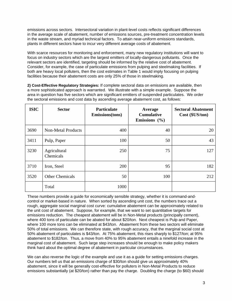
2) Cost-Effective Regulatory Strategies: If complete sectoral data on emissions are available, thena more sophisticated approach is warranted. We illustrate with a simple example. Suppose thearea in question has five sectors which are significant emitters of suspended particulates. We orderthe sectoral emissions and cost data by ascending average abatement cost, as follows:

ISIC Sector ParticulateEmissions(tons)

AverageCumulative

Emissions (%)

Sectoral AbatementCost ($US/ton)

3690 Non-Metal Products 400 40 20

3411 Pulp, Paper 100 50 43

3230 AgriculturalChemicals

250 75 127

3710 Iron, Steel 200 95 182

3520 Other Chemicals 50 100 212

Total 1000

These numbers provide a guide for economically sensible strategy, whether it is command-and-control or market-based in nature. When sorted by ascending unit cost, the numbers trace out arough, aggregate social marginal cost curve: cumulative abatement can be approximately related tothe unit cost of abatement. Suppose, for example, that we want to set quantitative targets foremissions reduction. The cheapest abatement will be in Non-Metal products (principally cement),where 400 tons of particulate can be abated for about $20/ton. Next cheapest is Pulp and Paper,where 100 more tons can be eliminated at $43/ton. Abatement from these two sectors will eliminate50% of total emissions. We can therefore state, with rough accuracy, that the marginal social cost at50% abatement of particulates is $43/ton. At 75% abatement, this rises sharply to $127/ton; at 95%abatement to $182/ton. Thus, a move from 40% to 95% abatement entails a ninefold increase in themarginal cost of abatement. Such large step increases should be enough to make policy makersthink hard about the optimal degree of abatement in particular circumstances.

We can also reverse the logic of the example and use it as a guide for setting emissions charges.Our numbers tell us that an emissions charge of $30/ton should give us approximately 40%abatement, since it will be generally cost-effective for polluters in Non-Metal Products to reduceemissions substantially (at $20/ton) rather than pay the charge. Doubling the charge (to $60) should

4

buy another 10% abatement. To effect 95% abatement the charge would have to be tripled again, tosomething over $182/ton.

We hope that these simple examples will suffice to illustrate the potential utility of our cost estimates.Complete information is included below, in Table 1.

Table 1: AVERAGE ABATEMENT COST BY SECTOR, 1979-1985 ($1993/ton)

ISIC Particulates SulfurOxides

NO2,CO2

Hydro-carbons

Lead Haz.Emission

s

Other

3110 Food 86 521 229 162 46612 55 55

3130 Beverages 156 271 11918 11918 76 76 76

3140 Tobacco 268 167 167 12030 128 128 167

3210 Textiles 396 396 1379 1379 1191 1191 1191

3211 Spinning 272 535 1431 188 781 188 188

3220 Apparel 445 61 61 61 61 61 61

3230 Leather 132 377 8430 633 132 324 427

3240 Footwear 540 207 993 1558 22141 1197 901

3310 Wood 47 38 38 38 38 38 38

3320 Furniture 43 25 25 25 24 13335 25

3410 Paper Products 87 364 472 472 87 87 87

3411 Pulp, Paper 43 155 20 20 35 35 35

3420 Printing 424 117 309 307 117 5604 117

3511 IndustrialChemicals

46 75 304 213 1300 311 206

3512 AgriculturalChemicals

127 519 889 341 532 1069 320

3513 Resins 82 562 207 123 435 63 264

3520 ChemicalProducts

212 681 48 157 29 29 204

5

ISIC Particulates SulfurOxides

NO2,CO2

Hydro-carbons

Lead Haz.Emission

s

Other

3522 Drugs 269 1045 451 173 300 300 300

3530 Refineries 328 165 59 121 2750 2750 2750

3540 Petroleum, Coal 59 1942 77 77 42 42 42

3550 Rubber 219 1107 343 343 1010 1010 1010

3560 Plastics 219 2415 235 235 1132 1132 1132

3610 Pottery 185 106 3792 3792 4709 4709 4709

3620 Glass 186 550 339 339 186 186 186

3690 Non-MetalProducts, n.e.c.

20 213 1647 1658 11 11 11

3710 Iron, Steel 182 528 115 1203 779 253 18

3720 Non-FerrousMetals

340 152 49 622 1284 1153 177

3810 Metal Products 343 1563 461 399 161 161 427

3820 Other Machinery 254 855 515 515 138 138 138

3825 Office, ComputingMachinery

245 245 864 937 248 17458 245

3830 Other ElectricalMachinery

373 483 1559 215 365 166 166

3832 Radio, TV 394 1854 904 1096 738 1491 1138

3840 TransportEquipment

635 1266 468 1006 468 2331 468

3841 Shipbuilding 125 832 2229 2229 84 84 84

3843 Motor Vehicles 350 1523 1155 2441 21483 159 159

3850 ProfessionalGoods

1208 3046 872 1376 995 1634 995

3900 Other Industries 38 26 110 110 26 26 26

6

The cost estimates in the Appendix Table 4.2 are in $1979. These have been inflated to $1993 forthis executive summary, using an annual compound rate of inflation of 4.6%. The latter wascomputed using fixed-weight price indices for pollution abatement and control for 1979 and 1989 andwas obtained from "Pollution Abatement and Control Expenditures, 1972-90", Survey of CurrentBusiness, June 1992.

1. Introduction

In this paper, we develop estimates of air pollution abatement costs for U.S. manufacturing sectors

at the four-digit level of International Standard Industrial Classification (ISIC). We utilize a very

large plant-level database for the period 1979-1985, a high point in industry response to the

abatement requirements of the U.S. Clean Air Act. Our estimates measure both marginal and

average total abatement costs for seven categories of air pollutants.3 As far as we know, they

provide the only consistent summary of abatement costs across all manufacturing sectors. As such,

they offer new information to policy makers who are concerned with evaluating the benefits and

costs of pollution control. The cost estimates also provide evidence on the relative economic

efficiency of command-and-control regulation, as practiced in the U.S. The greater the variation in

sectoral abatement costs for a given pollutant, the greater the inefficiency of the abatement efforts

for society at large.

In developing our estimates, we have used a model of joint pollutant abatement cost which is

discussed in Section 2. Section 3 describes the data, which have been created by merging plant-

level information from two sources: The U.S. Department of Commerce's annual 20,000-plant

random survey of pollution abatement costs and expenditures (PACE), and the U.S. Census

Bureau's Annual Survey of Manufactures.4 The PACE data for 1979-85 include reported pollutant

abatement and cost, while the Census provides detailed sectoral identifiers. In Section 4, we

3 These are particulates, sulfur oxides, nitrogen oxides and carbon monoxide, hydrocarbons, lead,hazardous air pollutants and a residual "Other" category.

4 While random sampling reduces the scope for assembling a panel of firms from PACE, it doesassure very broad representation over time. The estimates reported in this paper incorporate someinformation from approximately 100,000 facilities.

7

present our econometric results and the implied estimates of pollution abatement costs. Section 5

summarizes the paper.

2. The Abatement Cost Function

Until recently, the scarcity of appropriate plant-level data has prevented detailed empirical studies of

average and marginal abatement costs by pollutant.5 Policy analyses have frequently developed

abatement cost estimates from engineering models. However, failure to rely on behavioral data has

led to considerable estimation errors in some cases.6 This paper attempts to advance the state of

the art by analyzing plant-level data on end-of-pipe abatement and related costs.

2.1 Abatement Technology and Economics

End-of-pipe abatement volume is the difference between influent and effluent, where influent is the

waste water or gas from production before treatment and effluent is the residual emitted after

treatment. The presence of some pollutant in the waste stream registers as a concentration,

typically measured in µg/l3 for air emissions. From an engineering perspective, 'abatement' means

installing and operating processes which reduce influent concentrations from one or more sources to

target effluent concentrations. Box 1 (p. 5) includes illustrative descriptions for three pollution-

intensive industry sectors, while Table 2.1 (p. 6) provides complementary average abatement

volume and cost estimates from the Appendix tables.

The engineering literature identifies four major factors which determine the cost of abatement:

Pollutant type, diversity of emissions sources, scale of abatement, and pollutant concentration in the

5 For a recent exception see Mundle, et. al. (1994).

6 A useful illustration is provided by the trading price for SO2 emissions permits under the U.S.Clean Air Act (Hamilton, 1994). Using engineering models, the U.S. Government forecast a pricearound $600/ton before the trading system was instituted. In fact, permits are currently tradingaround $150/ton.

8

waste stream.7 When air emissions from industrial processes are concentrated at a few points,

most abatement can be accomplished using three basic systems:

• Dry systems use gravity, centrifugal force or fabric filters to trap pollutants. Gravity/centrifugalsystems are low-cost, but appropriate only for removal of relatively heavy particulates. Filtersystems trap fine particulates; costs vary widely according to waste stream characteristics anddesired removal rates.

• Wet scrubbers use streams of water or other liquids to increase collection efficiency. Wetcollectors can cool and wash waste streams and remove gases. High-efficiency systems havehigh operating costs. Scrubbers come in a great variety of sizes, configurations and efficiencylevels, depending on the problem. Their slurry can be a serious source of water pollution if it isdischarged because hazardous pollutants may be highly concentrated. Thus, additionaltreatment may be needed to complement the cleaning of air pollutants.

• Electrostatic precipitators use the principle of electrostatic attraction to trap pollutants bychanneling the waste stream between two electrodes - a high-voltage discharge electrode and agrounded collecting electrode. Plate precipitators allow for the dry collection of very fine particlesand are highly efficient. Pipe precipitators work better for liquid aerosols or fumes. In generalprecipitator systems have low maintenance costs, although dry systems are subject to explosiondangers if they are operated beyond rated capacity.

2.1.1 Pollutant-specific factors

Simpler, less energy-intensive collection systems are less efficient and generally suitable only for

large, dense particulates. Fine particulates and other air pollutants require more sophisticated,

costly collection devices. This difference can be seen, for example, in Table 2.1, where average

7 The discussion in this section (including Box 1) relies heavily on Sell (1992).

9

abatement costs for sulphur oxide removal are at least three times higher than those for

particulates.8

8 In some sectors, removal of fine particulates from diverse sources may increase abatement costssubstantially. As Table 1 indicates, sulphur oxide abatement costs by sector are generally, but notalways, higher than particulate abatement costs.

10

BOX 1: PRODUCTION PROCESSES AND EMISSIONS CONTROL INTHREE POLLUTION-INTENSIVE SECTORS

In this box we describe the basic processes and emissions control problems in three sectors: Iron and Steel, Pulpand Paper and Cement. All three sectors are extremely energy-intensive, and large installations frequentlymaintain their own power-generation facilities. When the latter burn fossil fuels, they have common controlproblems which focus on particulate and sulphur oxide removal. Sectoral abatement costs therefore reflect a mixof common costs from power plant emissions control and costs which reflect differences in sectoral productionprocesses.IRON AND STEEL

Pig Iron ProductionThe production of pig iron involves coking and blast furnace operation. During coking, there are many possibleemissions sources. SO2 and particulates are emitted into the atmosphere during charging (filling the oven), fromdoor and lid leaks, and from quenching the coke with wastewater. Coke oven gas is often burned for fuelelsewhere in the plant and can also produce these emissions.

Diverse emissions sources require diverse solutions: Oven lid and door maintenance; putting baffles in thequenching towers; using clean, not waste, water for the quenching process; stack gas cleaning of the SO2; usingnegative oven pressures during the charging; and hooding many of the steps to capture releases. In general, cokeoven emissions are very difficult to control.

Blast furnace operation produces primarily SO2 and CO. Sulphur in the coke oxidizes to form SO2, which escapesfrom the top of the furnace.

Steelmaking

Air pollution problems in this process come mostly from fume generation by the furnaces and from pouringoperations. Open hearth and basic oxygen units use electrostatic precipitators or venturi scrubbers to removeparticulates; newer electric furnaces use dry collection in bag houses (fabric filtering installations).

PULP AND PAPERSpecific environmental effects depend on the process used. Kraft (or sulfate) pulping processes are dominant inthe industry and produce most of the pollution. Kraft pulping uses chemicals, heat and pressure to dissolve thewood material. Sulphur-containing gases are released during this process; after concentration of waste 'liquor'into solid residuals, burning of the latter for organic residue removal also releases sulphurous waste gases. Mostplants use wet scrubbers to remove sulphur gases and particulates from the waste stream.

CEMENT

The major environmental problem for this sector is handling the waste kiln dust, particularly from plantsemploying wet processes. Dust removal is generally done with electrostatic precipitators.

11

Table 2.1

Average Abatement Volume and Cost for PACE Facilities

Average Abatement Volume

(Tons)

Sector ISIC Total Suspended

Particulates

Sulphur Oxides

Cement 3690 34,773 613

Pulp and Paper 3411 28,029 1,672

Iron and Steel 3710 12,336 1,108

Average Cost of Abatement

($US 1993/Ton)

Sector ISIC Total Suspended

Particulates

Sulphur Oxides

Cement 3690 20 213

Pulp and Paper 3411 43 155

Iron and Steel 3710 182 528

Source: Tables 1, 3.2 (Abatement volumes in Table 2.1 are means from non-missing cells inAppendix Table 3.2)

2.1.2 Diversity of emissions sources

A major problem for control costs arises when significant emissions sources are dispersed and

highly varied. For example, Box 1 describes the diversity of iron and steel emissions as compared

with those of pulp, paper and cement. The consequences are suggested in Table 2.1: Average

abatement costs for iron and steel are much higher than those for the other sectors.

12

2.1.3 Scale of abatement

Scale economies may apply to some abatement processes, yielding declines in marginal and

average cost as treatment volume increases. The impact of this factor seems clearly apparent for

Total Suspended Particulates in Table 2.1: Average abatement cost drops sharply as abatement

volume increases.

2.2 Joint Production of Abatement

Abatement is frequently a joint process, since both scrubbing and electrostatic precipitation systems

can be used to reduce influent concentrations for several pollutants at the same time. For example,

as noted in Box 1, stack scrubbers can be used to remove both TSP and SO2 from air emissions.

Even where separate equipment is called for, there may be common use of skilled and unskilled

labor, materials and energy.

Generally then, abatement can be characterized as a multiple-output process whose costs are

affected by diminishing returns, pollutant-specific technology requirements, scale economies, and

diseconomies associated with diversity of emissions sources.

2.3 Model Specification

Our regression model is specified in equation (1) below.

We assume that the abatement cost function is separable from the firm's production cost function,reflecting purely end-of-pipe activity.9 In light of the preceding discussion, we estimate separateregressions by sector, using sectoral identification as our control for the influence of manyunobservable factors: Influent concentration, differential reduction of influent, abatement scale,source diversity, and more detailed engineering considerations. The quadratic specification of thecost function allows for testing possible pollutant-specific scale economies.

9 The PACE survey attempts to maintain this distinction, and we think that our assumption is areasonable approximation. However, it will not hold true in all cases. For example, the descriptionof iron and steel production in Box 1 notes the importance of costly adjustments such as negativeoven pressure for the reduction of emissions. In such cases, there is clearly some interactionbetween processing and abatement costs.

13

(1)

where:

Total cost of abatement for end - of - pipe air pollution control by plant i in sector j

= Quantity of air pollutant k abated by plant i

= A random disturbance term

ij j i jk ijk i jjk ijk ij

ij

ijk

ij

C

C

A A

A

= + + +

=

β β β ε

ε

02Σ Σ

There are various techniques for allocating the fixed cost component ( 0) in (1) across pollutants to

yield average cost estimates. We opt for the simplest in this paper, averaging the joint and common

cost across the sum (in tons) of all pollutants abated.10 Sectoral marginal and average costs are

therefore computed as follows:

(2a) MC Ajk jk jjk ijk= +β β2

(2b) AFC (A plant - level mean abatement of k)jk ijk= =β0 j k ijkA/ Σ

(2c) AC jk = + = + +MC AFC A Ajk jk jk jjk ijk j k ijkβ β β2 0 0/ Σ

We estimate Equation (1) for two sets of pollutant categories, depending on data availability. During

the period 1979-1982, PACE aggregated air pollutants into four categories:

1) particulates; 2) sulfur oxides; 3) nitrogen oxides, carbon monoxide and hydrocarbons; and 4) other

pollutants, including lead and toxic emissions. During 1983-1985, pollutants were surveyed in seven

categories: 1) particulates; 2) sulfur oxides; 3) nitrogen oxides and carbon monoxide; 4)

hydrocarbons; 5) lead; 6) hazardous emissions; 7) other.

We also test whether we can pool the data over 1979-1985. This pooling involves aggregating the

seven categories to the four categories for the 1983-1985 period. We test whether we can pool the

pollutants in both linear and quadratic forms of equation (1). For sectors in which we cannot reject

10 An alternative method would be to allocate joint and common costs among pollutants abated inproportion to their variable costs. This approach is called "axiomatic cost analysis." See forexample Mirman, Samet and Tauman (1983).

14

pooling by pollutant category over 1983-1985, we gain efficiency by estimating the equation for the

four categories over the whole period 1979-1985.

Because our focus is on internationally-comparable estimates, we have recoded all U.S. plants to

ISIC (International Standard Industrial Classification) categories using a concordance made available

by the U.S. Census Bureau. Our data set provides observations on Cij and Aijk for a large sample

of plants within each ISIC. We express all costs in U.S. 1979 dollars; volumes are in tons.11 We

estimate the regression equations using OLS, because command-and-control regulation has forced

U.S. plants toward similar effluent concentrations with little regard for relative abatement costs.

Several WLS corrections have been tested and rejected.

3. Econometric Issues -- Data and Estimation

Since the 1970's, the United States Department of Commerce has implemented an annual survey of

pollution abatement costs and expenditures (PACE).12 The survey summarizes annual capital and

operating costs of abatement for a random sample of approximately 20,000 establishments

identified at the four-digit SIC level.13 The PACE data also record annual abatement volumes for

many air, water and solid waste pollutants. In this paper, we focus on the air pollutants.14

11 Note that the regressions reported in Tables 4.1 and 4.2 were run on data adjusted to constant$US 1979. These results are inflated to $US 1993 for presentation in the Executive Summary (Table1).

12 The annual survey continues, but its scope and relevance were seriously compromised in 1986 bythe elimination of questions on abatement volumes. We are therefore unable to exploit more recentPACE data for the work reported in this paper.

13 Specifically, the annual operating expenses include the cost of capital services in the form ofdepreciation; labor costs; materials, supplies, fuel and electricity; and contracted services,equipment, leasing and other. The survey also quantifies annual capital expenditures for abatementequipment.

14 Regression-based estimates for the major regulated water pollutants are also available from theauthors on request.

15

We have used common identifier numbers to merge the PACE data with the Longitudinal Research

Database (LRD) of the US Bureau of the Census.15 The LRD pools annual data at the establishment

level from the U.S. Census of Manufactures and the Annual Survey of Manufactures. It includes

detailed information on location; ownership; inputs (labor, energy, materials, plant and equipment);

and production of goods and services at a highly disaggregated level. For this study, we have used

the LRD only for sectoral identification of the PACE facilities.

We have translated the U.S. coding of our sample establishments (4-digit SIC) into 37 four-digit ISIC

categories. The latter are listed in Appendix Table 3.1. For each sector and pollutant category,

Appendix Table 3.2 displays mean tons abated during the periods 1979-1982 and 1983-1985. These

estimates reflect abatement by the representative establishment in each ISIC. Volumes for the

chemical and resource processing industries (ISIC 3411 - 3690) are particularly noteworthy for most

air pollutants. The more disaggregated information for 1983-1985 makes it clear that lead and some

hazardous air pollutants have small average volumes at the plant level.

4. Results

Because the complete results for all 37 ISIC industries are quite lengthy, we do not discuss them in

detail here. Full results are available from the authors on request. In this section, we present

estimates of marginal and average total abatement costs for cases where statistically significant

regression coefficients have been obtained. These cost estimates are provided in Appendix Tables

4.1 and 4.2. Separate cost estimates are presented for 1979-1982, 1983-1985 and (where pooling

cannot be rejected) 1979-1985. Cost estimates are always presented for all seven pollutants

(denoted P1 - P7). In the four-pollutant cases, cost estimates for the aggregate categories are

15 See McGuckin and Pascoe (1988).

16

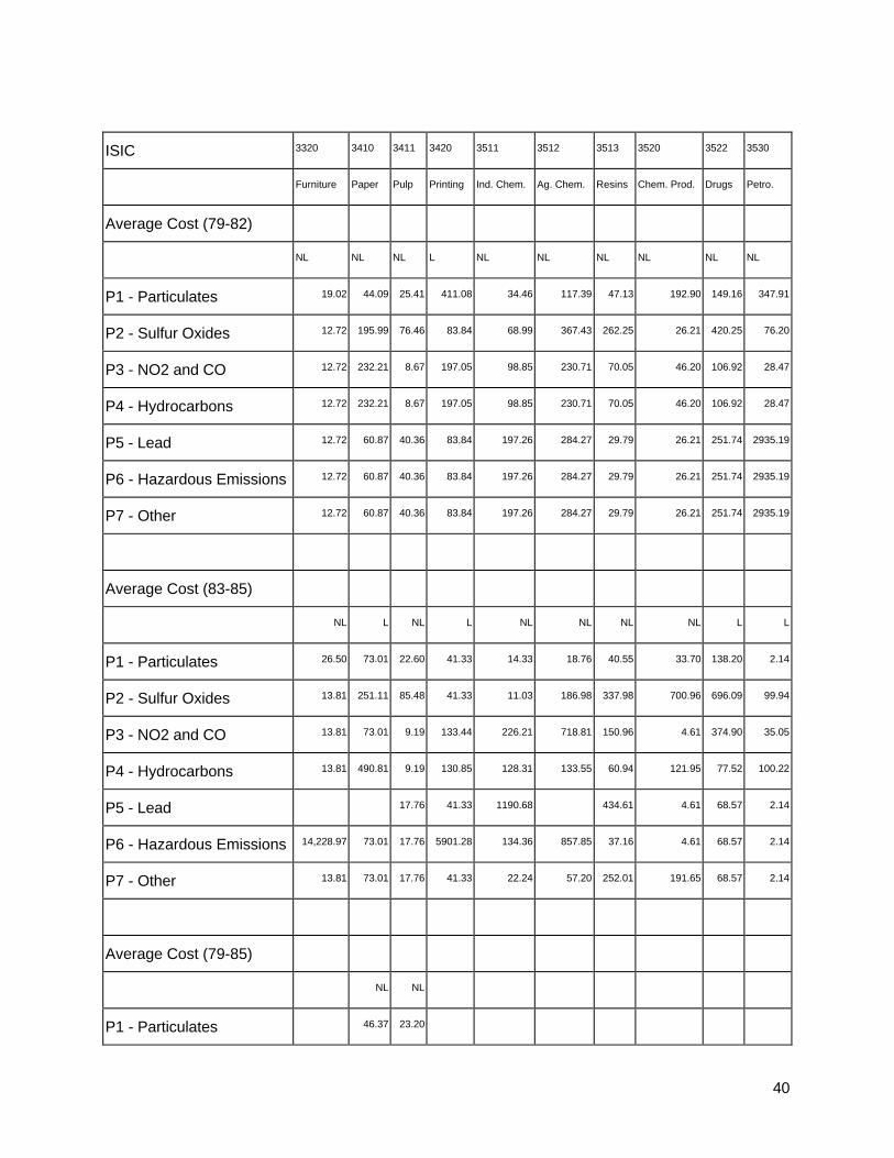
assumed constant across the constituent pollutants.16 Tables 4.1 and 4.2 also identify whether the

linear or non-linear version of the cost function is reported.17

Several conclusions can be drawn from Table 4.1. First, many sectors have nonlinear abatement

cost functions. Some marginal costs rise with abatement (due to the technological difficulty of

increasing abatement rates), while others fall (due, presumably, to the scale effect once some

threshold level of abatement is achieved).

Second, we accept the pooling hypothesis (and associated pooled cost estimates) for approximately

30% of the industries (3130, 3210, 3310, 3410, 3411, 3540, 3610, 3620, 3820, 3841 and 3900 -- see

Table 3.1).18

Third, marginal abatement costs vary considerably by pollutant and sector. Notice, for example, that

marginal costs for ISIC 3610 range from $69.04 for particulates to $2484.90 for lead, hazardous air

pollutants and other pollutants. These costs are substantially less for ISICs 3410 and 3411.

Fourth, the separate estimates for 1979-1982 and 1983-1985 reveal a very broad pattern of

variation. For some sectors and some pollutants, marginal abatement costs decline over time (e.g.,

particulates in 3211 and 3520 and sulphur oxides in 3512). For other sectors and pollutants, marginal

costs rise with time, perhaps reflecting scale effects or (more likely) changes in subsectoral

composition of plants surveyed (e.g., 3511: nitrogen oxides plus carbon monoxide; hydrocarbons).

16 For example, the estimated costs for the third category of pollutant will apply to both P3 and P4,while the estimated costs for the fourth category will apply to P5, P6 and P7.

17 The choice of linear or non-linear version is determined by the relative statistical performance ofeach. In a few cases, the version that was selected on overall statistical merit (that is, across allpollutants simultaneously) did not produce a usable cost estimate for a given pollutant. In suchcases, we report the pollutant-specific cost estimate from the relevant "next-best" regression.

18 Where pooling cannot be rejected, these estimates are the most efficient.

17

In both cases, the changes are probably due to some combination of technical change, scale effects

and alteration in subsectoral composition.

Many estimates are not statistically distinct.19 In some cases, estimates seem affected by small

sample sizes or joint abatement costs which are far larger than abatement quantities for particular

pollutants. For example, the marginal cost estimates for lead and hazardous air pollutants are quite

large for some sectors (e.g., 3110, 3320, 3843, and 3900).

Fifth, we should note that separate regressions for individual years (1979 through 1985) did not yield

generally robust results and are not reported.

Finally, we report the results of a fixed effects regression of marginal abatement costs for all

establishments whose sole

pollutant was particulates. Pooling of these establishments increases degrees of freedom and

estimation efficiency considerably. Our fixed effects model allows for slope and intercept dummies

for establishments in each ISIC. For this simpler abatement function, our results suggest that the

marginal cost of abatement is fairly constant at approximately $5.54/ton for many sectors. Some

sectors do reveal distinct abatement problems with much higher marginal costs (e.g., ISIC 3140 =

$61.17; ISIC 3530 = $98.75; and ISIC 3843 = $81.24). The estimates of average total abatement

cost in Table 4.2 extend these interpretations, but remain consistent with them.

5. Summary and Conclusions

In this paper, we have estimated the costs of abating major air pollutants. Our results reveal very

high variances in abatement costs for individual pollutants by sector: maximum/ minimum ratios are

19 We do not test statistically whether the cost estimates differ across the two periods.

18

frequently near ten, and occasionally near one hundred. They also show large differences in the

means and variances of costs across pollutants.

For environmental policymakers, these results suggest an important lesson: Command-and-control

(CAC) regulation in the U.S. seems to have reduced pollution at a very high cost. Optimal regulation

would attain the desired reduction in pollution while equalizing the marginal cost of abatement across

sectors. Where they are feasible, market-based instruments such as emissions charges and

tradable permits are optimal in this sense. In principle, regulators who were properly informed about

abatement costs could approach this optimum using CAC-type methods. In practice, we can see

that nothing like this has occurred. For the same pollutant, intersectoral abatement costs can differ

by more than a factor of 100.

While command-and-control regulation has certainly not been optimal for the U.S., it has undeniably

been useful for this exercise. By forcing roughly uniform emissions standards on sectors with very

different pollution control problems, it has permitted us to estimate intersectoral differences in costs.

These are so large that environmental policy-makers would be unwise to ignore them. Table 1

provides our current best estimates of average abatement costs by sector and pollutant.20 When

combined with information on the main sectoral sources of air pollution in a particular region, Table 1

can be used as a guide to setting priorities for pollution control. Since regulatory resources are

scarce, it undoubtedly makes sense to focus initial efforts on those sectors characterized by

relatively large contributions to total emissions and relatively low average costs of abatement.

20 These estimates come from Table 4.2 and are inflated to $1993, as discussed in the ExecutiveSummary.

19

Table 3.1

Industry Sectors

(International Standard Industrial Classification)

ISIC SECTOR

311 Food Products

313 Beverages

314 Tobacco

321 Other Textile Products

321 Spinning, Weaving

322 Wearing Apparel

323 Leather & Products

324 Footwear

331 Wood Products

332 Furniture, Fixtures

341 Other Paper Products

341 Pulp, Paper

342 Printing, Publishing

351 Other Industrial Chemicals

351 Basic Industrial Chemicals

351 Agricultural Chemicals

351 Synthetic Resins

352 Other Chemical Products

352 Drugs and Medicines

353 Petroleum Refineries

354 Petroleum & Coal Products

355 Rubber Products

20

ISIC SECTOR

356 Plastic Products

361 Pottery, China, etc.

362 Glass & Products

369 Non-Metal Products n.e.c.

371 Iron and Steel

372 Non-Ferrous Metals

381 Metal Products

382 Other Machinery n.e.c.

382 Office & Computing Machinery

383 Other Electrical Machinery

383 Radio, Television, etc.

384 Transport Equipment

384 Shipbuilding, Repair

384 Motor Vehicles

385 Professional goods

390 Other Industries

21

REFERENCES

Dollar, D., 1992, "Outward-Oriented Developing Economies Really Do Grow More Rapidly: Evidencefrom 9 LDCs, 1976-1985,"

Economic Development and Cultural Change, pp. 523-544.

Hamilton, M., 1994, "Selling Pollution Rights Cuts the Cost of Cleaner Air," Washington Post, August24, p. F1.

McGuckin, R.H. and G. A. Pascoe, 1988, "The Longitudinal Research Database: Status andResearch Possibilities," in Bureau of Economic Analysis, US Department of Commerce, Survey ofCurrent Business, November.

Mirman, L.J, D. Samet and Y. Tauman, 1983, "An Axiomatic Approach to the Allocation of a FixedCost Through Prices," Bell Journal of Economics, 14(1).

Mundle, S., S. Mehta and U. Shankar, 1994, "Incentives and Regulation for Pollution Abatement,With an Application to Waste Water Treatment," paper presented to the 50th Congress of theInternational Institute of Public Finance, August 25-29, Harvard University.

Sell, N., 1992, Industrial Pollution Control: Issues and Techniques (New York: Van Nostrand)

22

Table 3.2 Mean Tons Abated

ISIC 3110 3130 3140 3210 3211 3220 3230 3240 3310

Food Beverages Tobacco Textile Spinning Apparel Leather Footwear Wood

P1 - Particulates

Four Pollutants 1979-1982 1474.9 2770.8 1348.9 93.3 574.7 134.7 18.1 2345.5

Four Pollutants 1983-1985 1170.0 163.3 2333.5

Seven Pollutants 1983-1985 1429.3 1170.0 1968.0 163.3 658.6 252.4 13.4 2333.5

P2 - Sulfur Oxides

Four Pollutants 1979-1982 56.2 144.7 41.2 3.3 9.1 14.3 0.1 6.5

Four Pollutants 1983-1985 107.0 1.8 2.5

Seven Pollutants 1983-1985 40.6 107.0 34.8 1.8 28.2 1.4 2.5

P3 - NO2 and CO

Four Pollutants 1979-1982 165.7 1.8 15.6 112.9 37.7 11.8 0.7 23.2

Four Pollutants 1983-1985 9.4 142.1 56.0


P4 - Hydrocarbons

Four Pollutants 1979-1982 13.7 25.0 15.0 20.9 13.3 0.4 0.2 14.1

Four Pollutants 1983-1985 0.3 16.1 71.6


P5 - Lead

Four Pollutants 1979-1982


23

Seven Pollutants 1983-1985 0.1 3.7 0.01 0.008 0.002

P6 - Hazardous Emissions



Seven Pollutants 1983-1985 0.4 15.4 2.5 5 0.2 0.8

P7 - Other




24

ISIC 3320 3410 3411 3420 3511 3512 3513 3520 3522 3530

Furniture Paper Pulp Print. Ind. Chem. Ag. Chem. Resins Chem. Prod. Drugs Petro.

P1 - Particulates

Four Pollutants 1979-1982 2756.5 1382.8 26565.4 39.0 7353.6 1296.8 4820.0 463.2 977.6 1906.1

Four Pollutants 1983-1985 37.3 28760.5 197.7 447.1

Seven Pollutants 1983-1985

2047.8 37.3 28760.5 197.7 242784.4 1350.5 4783.7 738.2 447.1 1851.4

P2 - Sulfur Oxides

Four Pollutants 1979-1982 3.3 75.6 1837.3 0.2 1879.8 311.8 118.8 40.0 265.8 26687.8

Four Pollutants 1983-1985 24.9 1589.6 0.2 81.8


2.5 24.9 1589.6 0.2 69102.0 654.4 82.0 24.6 81.8 33267.2

P3 - NO2 and CO

Four Pollutants 1979-1982 31.6 268.4 305.1 696.4 3205.8 1237.0 2233.9 1792.5 318.2 49095.3

Four Pollutants 1983-1985 6.5 379.6 1518.0 526.6


77.8 0.1 318.7 397.2 1583.2 270.0 217.7 11257.5 12.4 38138.4

P4 - Hydrocarbons

Four Pollutants 1979-1982 22.3 17.0 1002.5 2.4 876.6 383.2 165.1 46.3 68.9 1182.8

Four Pollutants 1983-1985 3.7 1044.7 19.1 184.6


5.2 6.4 60.8 1120.8 1656.0 824.5 1911.3 1003.4 514.2 10044.6

P5 - Lead

25




0.1 17.7 6.5 0.8 0.3 73.6





0.2 0.03 27.3 0.2 216.1 22.8 605.3 9.7 1.8 142.6

P7 - Other




11.5 3.7 1017.3 18.9 1011.1 1285.3 63.4 1142.9 182.5 79.6

26

ISIC 3540 3550 3560 3610 3620 3690 3710 3720 3810

Coal Rubber Plastic Pottery Glass N-Metal Iron N-Ferrous Metal Metal

P1 - Particulates

Four Pollutants 1979-1982 3777.0 525.2 290.0 408.0 508.2 34936.0 15205.6 4530.3 225.0

Four Pollutants 1983-1985 2623.8 581.5 508.4 685.9 34690.6


P2 - Sulfur Oxides

Four Pollutants 1979-1982 42.7 63.5 2.8 0.1 29.2 257.0 796.2 5527.9 7.0

Four Pollutants 1983-1985 33.6 37.1 0.03 15.4 791.6


P3 - NO2 and CO

Four Pollutants 1979-1982 1919.9 89.0 132.2 6.3 27.8 81.5 3299.3 154.5 123.0

Four Pollutants 1983-1985 1527.4 70.2 12.4 61.7 223.2


P4 - Hydrocarbons

Four Pollutants 1979-1982 3.3 40.7 35.3 0.2 7.3 353.8 800.6 724.5 21.5

Four Pollutants 1983-1985 0.3 3.6 4.8 10 102.5


P5 - Lead



27






P7 - Other




28

ISIC 3820 3825 3830 3832 3840 3841 3843 3850 3900

Machinery Computing Electrical Radio Transport Ships Vehicles P. Goods Other

P1 - Particulates

Four Pollutants 1979-1982 404.0 109.9 583.2 186.2 159.9 420.9 1022.1 23.8 245.4

Four Pollutants 1983-1985 203.5 204.0 1080.5

Seven Pollutants 1983-1985 203.5 72.3 399.6 101.5 178.8 204.0 547.4 28.7 1080.5

P2 - Sulfur Oxides

Four Pollutants 1979-1982 62.6 5.2 31.0 8.0 55.0 185.4 120.2 1.2 0.2

Four Pollutants 1983-1985 48.7 141.7 0.3


P3 - NO2 and CO

Four Pollutants 1979-1982 37.0 211.3 168.8 148.7 27.6 28.1 139.9 17.4 7.8

Four Pollutants 1983-1985 26.0 28.8 444.7


P4 - Hydrocarbons

Four Pollutants 1979-1982 30.1 4.7 84.8 16.0 7.3 13.4 407.2 2.8 10.1

Four Pollutants 1983-1985 7.1 1.9 1376.4


P5 - Lead


29







P7 - Other




30

Table 4.1: Marginal Abatement Costs ($1979)

ISIC 3110 3130 3140 3210 3211 3220 3230 3240 3310


Marginal Cost (79-82) NL L NL NL L L L L

P1 - Particulates 14.77 107.90 405.62 49.38 204.95 261.67 72.11 5.47

P2 - Sulfur Oxides 381.28 4777.57 370.80 311.11

P3 - NO2 and CO 2.99 187.24 92.52 311.11 555.38

P4 - Hydrocarbons 2.99 187.24 92.52 555.38

P5 - Lead 490.00 20.28

P6 - Hazardous Emissions 490.00 20.28

P7 - Other 490.00 20.28

Marginal Cost (83-85) L NL L NL L NL

P1 - Particulates 17.82 39.69 14.38

P2 - Sulfur Oxides 116.54

P3 - NO2 and CO 182.77 698.99 1327.18 8550.88

P4 - Hydrocarbons 111.01 12669.50 712.09 453.33 223.47 603.73

P5 - Lead 49,723.02 633.16 23,142.34

P6 - Hazardous Emissions 747.32 191.06 773.40

P7 - Other 300.10 457.51

Marginal Cost (79-85) NL NL L

P1 - Particulates 42.42 4.78

P2 - Sulfur Oxides 103.91

P3 - NO2 and CO 6323.80 524.76

31

P4 - Hydrocarbons 6323.80 524.76

P5 - Lead 424.44

P6 - Hazardous Emissions 424.44

P7 - Other 424.44

Marginal Cost (79-85)

P1 - Particulates* 5.54 5.54 61.17 5.54 35.62 223.58 5.54 5.54 5.45

*(Particulates only)

** L - Linear, NL - Non-Linear

32

ISIC 3320 3410 3411 3420 3511 3512 3513 3520 3522 3530

Furniture Paper Pulp Printing Ind. Chem. Ag. Chem. Resins Chem. Prod. Drugs Petro.

Marginal Cost (79-82) NL NL NL L NL NL NL NL NL NL

P1 - Particulates 6.30 26.58 16.74 327.23 7.83 45.24 17.34 166.69 115.20 336.43

P2 - Sulfur Oxides 178.48 67.79 42.36 295.28 232.46 386.29 64.72

P3 - NO2 and CO 214.70 113.21 72.22 158.56 40.26 19.99 72.96 16.99

P4 - Hydrocarbons 214.70 113.21 72.22 158.56 40.26 19.99 72.96 16.99

P5 - Lead 43.36 31.69 170.63 212.12 217.78 2923.71

P6 - Hazardous Emissions 43.36 31.69 170.63 212.12 217.78 2923.71

P7 - Other 43.36 31.69 170.63 212.12 217.78 2923.71

Marginal Cost (83-85) NL L NL L NL NL NL NL L L

P1 - Particulates 12.69 13.41 13.42 19.77 29.09 69.63

P2 - Sulfur Oxides 1620.60 178.14 76.29 92.11 10.12 168.22 317.20 696.35 627.51 97.80

P3 - NO2 and CO 417.86 89.52 225.30 700.05 130.18 306.33 32.91

P4 - Hydrocarbons 417.86 127.40 114.79 40.19 117.34 6.95 98.07

P5 - Lead 8.57 5859.95 1189.70 413.83

P6 - Hazardous Emissions 14,215.16 8.57 133.45 839.09 7.52

P7 - Other 8.57 20.56 38.44 231.23 187.04

Marginal Cost (79-85) NL NL


P2 - Sulfur Oxides 176.83 72.12

P3 - NO2 and CO 234.39

P4 - Hydrocarbons 234.39

33

P5 - Lead 28.79 8.08


P7 - Other 28.79 8.08


P1 - Particulates* 5.45 5.54 5.54 5.54 1.65 5.54 5.54 5.54 5.54 98.75

34

ISIC 3540 3550 3560 3610 3620 3690 3710 3720 3810

Coal Rubber Plastic Pottery Glass N-Metal Iron N-Ferrous Metal Metal

Marginal Cost (79-82) NL NL NL NL L NL NL NL NL

P1 - Particulates 10.89 52.44 84.01 166.01 4.51 77.10 173.27 101.46

P2 - Sulfur Oxides 1914.63 312.98 1256.79 205.14 138.36 539.79 64.55 949.68

P3 - NO2 and CO 8.79 169.15 92.44 2134.64 128.48 911.98 69.34 135.69

P4 - Hydrocarbons 8.79 169.15 92.44 2134.64 128.48 911.98 69.34 135.69

P5 - Lead 343.54 571.43 136.91


P7 - Other 343.54 571.43 136.91

Marginal Cost (83-85) NL NL NL NL NL NL NL NL

P1 - Particulates 7.21 33.72 4.60 97.60 137.55 93.48

P2 - Sulfur Oxides 227.32 308.30 77.06 4.32 45.14 547.53

P3 - NO2 and CO 44.03 5907.00 220.22 835.36 33.34 184.63

P4 - Hydrocarbons 18.91 2662.79 196.34 847.33 1195.59 612.08 119.11

P5 - Lead 22,536.78 811.80 1182.05


P7 - Other 1127.01 3667.96 284.14

Marginal Cost (79-85) NL NL NL L

P1 - Particulates 9.25 25.18 69.04

P2 - Sulfur Oxides 1014.70 498.96 194.69

P3 - NO2 and CO 18.78 93.99 1994.90 81.61

P4 - Hydrocarbons 18.78 93.99 1994.90 81.61

35

P5 - Lead 447.48 2484.90


P7 - Other 447.48 2484.90


P1 - Particulates* 5.54 5.54 5.54 5.54 5.54 3.25 64.54 5.54 53.32

36

3820 3825 3830 3832 3840 3841 3843 3850 3900

Machinery Computing Electrical Radio Transport Ships Vehicles P. Goods Other

Marginal Cost (79-82) NL NL NL NL L NL NL NL NL

P1 - Particulates 52.15 110.01 39.04 50.96 126.89 264.90 5.77

P2 - Sulfur Oxides 425.83 408.46 1718.26 427.70 374.17 1354.92 2632.73

P3 - NO2 and CO 294.98 661.33 81.64 513.09 1618.58 1080.98 65.57 134.69

P4 - Hydrocarbons 294.98 661.33 81.64 513.09 1618.58 1080.98 65.57 134.69

P5 - Lead 69.93 526.38 17.41 442.22

P6 - Hazardous Emissions 69.93 526.38 17.41 442.22

P7 - Other 69.93 526.38 17.41 442.22

Marginal Cost (83-85) NL L NL NL NL NL NL NL L

P1 - Particulates 89.93 181.63 117.81 127.41 334.01 221.47 359.63 13.32

P2 - Sulfur Oxides 288.53 424.62 632.50 118.80

P3 - NO2 and CO 122.32 1476.22 190.17 520.62 193.09

P4 - Hydrocarbons 198.34 78.24 40.49 395.21 574.13 1393.42 783.15 33.66

P5 - Lead 213.00 22738.60 3855.22

P6 - Hazardous Emissions 18384.10 803.70 1989.31 682.11 119.65

P7 - Other

Marginal Cost (79-85) NL L L

P1 - Particulates 62.,29 21.93 6.22


P3 - NO2 and CO 201.42 1145.40 44.67

P4 - Hydrocarbons 201.42 1145.40 44.67

37

P5 - Lead


P7 - Other


P1 - Particulates* 36.80 5.54 76.00 5.54 49.25 5.54 81.24 5.54 5.54

38

Table 4.2 Total Average Abatement Costs ($1979)

ISIC 3110 3130 3140 3210 3211 3220 3230 3240 3310


Average Cost (79-82)

NL L NL NL L L L L

P1 - Particulates 47.62 176.41 612.99 160.77 237.58 109.40 182.42 25.84

P2 - Sulfur Oxides 414.13 68.51 4984.94 482.19 32.63 371.07 110.31 20.37

P3 - NO2 and CO 35.84 68.51 394.61 111.39 32.63 420.51 665.69 20.37

P4 - Hydrocarbons 35.84 68.51 394.61 111.39 32.63 420.51 665.69 20.37

P5 - Lead 32.85 68.51 697.37 111.39 32.63 109.40 110.31 20.37

P6 - Hazardous Emissions 32.85 68.51 697.37 111.39 32.63 109.40 110.31 20.37

P7 - Other 32.85 68.51 697.37 111.39 32.63 109.40 110.31 20.37


NL L NL L NL L L

P1 - Particulates 43.99 110.06 177.46 129.36 31.95 394.51 23.44

P2 - Sulfur Oxides 142.65 110.06 177.46 89.67 31.95 20.32

P3 - NO2 and CO 208.88 110.06 177.46 1416.86 8582.83 394.51 20.32

P4 - Hydrocarbons 137.12 12,779.56 889.55 89.67 255.42 998.51 20.32

P5 - Lead 49,749.13 722.82 31.95 23,536.85 20.32


P7 - Other 26.11 110.06 177.46 89.67 346.14 852.02 20.32


NL NL L

39

P1 - Particulates 83.08 211.59 24.87

P2 - Sulfur Oxides 144.57 211.59 20.09

P3 - NO2 and CO 6364.46 736.35 20.09

P4 - Hydrocarbons 6364.46 736.35 20.09

P5 - Lead 40.65 636.03 20.09


P7 - Other 40.65 636.03 20.09


P1 - Particulates* 5.55 5.79 61.84 7.08 35.76 226.54 7.59 20.22 5.56

*(Particulates only)

** L - Linear, NL - Non-Linear

40

ISIC 3320 3410 3411 3420 3511 3512 3513 3520 3522 3530

Furniture Paper Pulp Printing Ind. Chem. Ag. Chem. Resins Chem. Prod. Drugs Petro.


NL NL NL L NL NL NL NL NL NL

P1 - Particulates 19.02 44.09 25.41 411.08 34.46 117.39 47.13 192.90 149.16 347.91

P2 - Sulfur Oxides 12.72 195.99 76.46 83.84 68.99 367.43 262.25 26.21 420.25 76.20

P3 - NO2 and CO 12.72 232.21 8.67 197.05 98.85 230.71 70.05 46.20 106.92 28.47

P4 - Hydrocarbons 12.72 232.21 8.67 197.05 98.85 230.71 70.05 46.20 106.92 28.47

P5 - Lead 12.72 60.87 40.36 83.84 197.26 284.27 29.79 26.21 251.74 2935.19

P6 - Hazardous Emissions 12.72 60.87 40.36 83.84 197.26 284.27 29.79 26.21 251.74 2935.19

P7 - Other 12.72 60.87 40.36 83.84 197.26 284.27 29.79 26.21 251.74 2935.19


NL L NL L NL NL NL NL L L

P1 - Particulates 26.50 73.01 22.60 41.33 14.33 18.76 40.55 33.70 138.20 2.14

P2 - Sulfur Oxides 13.81 251.11 85.48 41.33 11.03 186.98 337.98 700.96 696.09 99.94

P3 - NO2 and CO 13.81 73.01 9.19 133.44 226.21 718.81 150.96 4.61 374.90 35.05

P4 - Hydrocarbons 13.81 490.81 9.19 130.85 128.31 133.55 60.94 121.95 77.52 100.22

P5 - Lead 17.76 41.33 1190.68 434.61 4.61 68.57 2.14

P6 - Hazardous Emissions 14,228.97 73.01 17.76 5901.28 134.36 857.85 37.16 4.61 68.57 2.14

P7 - Other 13.81 73.01 17.76 41.33 22.24 57.20 252.01 191.65 68.57 2.14


NL NL


41


P3 - NO2 and CO 251.91 10.52

P4 - Hydrocarbons 251.91 10.52

P5 - Lead 46.31 18.60


P7 - Other 46.31 18.60


P1 - Particulates* 5.61 6.20 5.57 9.79 1.74 8.70 5.61 5.74 8.94 99.09

42

ISIC 3540 3550 3560 3610 3620 3690 3710 3720

Coal Rubber Plastic Pottery Glass N-Metal Iron N-Ferrous Metal


NL NL NL NL L NL NL NL

P1 - Particulates 30.82 104.55 116.85 166.01 136.15 11.36 88.37 195.10

P2 - Sulfur Oxides 1934.56 365.09 1289.63 341.29 145.21 551.07 86.38

P3 - NO2 and CO 28.72 221.26 125.28 2134.64 264.63 918.83 80.62 21.83

P4 - Hydrocarbons 28.72 221.26 125.28 2134.64 264.63 918.83 80.62 21.83

P5 - Lead 19.93 395.65 604.27 136.15 6.85 11.28 158.74

P6 - Hazardous Emissions 19.93 395.65 604.27 136.15 6.85 11.28 158.74

P7 - Other 19.93 395.65 604.27 136.15 6.85 11.28 158.74


NL NL NL NL NL NL NL

P1 - Particulates 33.82 126.91 36.04 73.97 9.52 106.03 167.85

P2 - Sulfur Oxides 253.93 401.49 36.04 73.97 81.98 12.75 75.44

P3 - NO2 and CO 70.64 93.19 5943.04 294.19 840.28 41.77 30.30

P4 - Hydrocarbons 45.52 93.19 2698.84 270.32 852.25 1204.02 642.38

P5 - Lead 26.61 93.19 36.04 22,610.75 4.92 820.23 1212.35


P7 - Other 26.61 1246.42 3704 73.97 4.92 8.43 30.30


NL NL NL NL

P1 - Particulates 31.76 117.12 98.88 99.21

43

P2 - Sulfur Oxides 1037.21 590.90 56.38 293.90

P3 - NO2 and CO 41.29 183.24 2024.74 180.82

P4 - Hydrocarbons 41.29 183.24 2024.74 180.82

P5 - Lead 22.51 539.42 2514.74 99.21

P6 - Hazardous Emissions 22.51 539.42 2514.74 99.21

P7 - Other 22.51 539.42 2514.74 99.21


P1 - Particulates* 5.82 5.87 7.78 6.67 5.83 3.26 64.57 5.85

44

ISIC 3810 3820 3825 3830 3832 3840 3841 3843 3850 3900

Metal Machinery Computing Electrical Radio Transport Ships Vehicles P. Goods Other


NL NL NL NL NL L NL NL NL L

P1 - Particulates 184.94 112.92 132.23 155.45 136.63 349.35 166.57 79.19 606.53 74.19

P2 - Sulfur Oxides 1033.16 486.60 132.23 453.90 1815.85 726.09 413.85 1434.11 2974.36 68.43

P3 - NO2 and CO 219.17 355.75 793.56 127.08 610.68 298.39 1658.26 1160.17 407.20 203.12

P4 - Hydrocarbons 219.17 355.75 793.56 127.08 610.68 298.39 1658.26 1160.17 407.20 203.12

P5 - Lead 83.48 60.77 132.23 115.37 623.97 298.39 39.68 96.60 783.85 68.43

P6 - HazardousEmissions

83.48 60.77 132.23 115.37 623.97 298.39 39.68 96.60 783.85 68.43

P7 - Other 83.48 60.77 132.23 115.37 623.97 298.39 39.68 96.60 783.85 68.43


NL NL L NL NL NL NL NL NL L

P1 - Particulates 181.67 183.20 129.10 243.42 284.02 329.03 412.34 294.69 683.61 21.59

P2 - Sulfur Oxides 635.72 381.80 129.10 61.79 164.51 626.24 674.36 192.02 278.98 8.27

P3 - NO2 and CO 272.82 218.26 129.10 1538.01 354.68 201.62 598.95 73.22 524.06 8.27

P4 - Hydrocarbons 207.30 291.61 207.34 102.28 559.72 775.75 78.33 1446.64 1062.13 41.93

P5 - Lead 88.19 93.27 274.79 164.51 201.62 78.33 22,847.82 278.98 3863.50


88.19 93.27 18,513.25 61.79 968.21 2190.93 78.33 73.22 961.09 126.34

P7 - Other 372.33 93.27 129.10 61.79 591.86 201.62 78.33 73.22 278.98 6.69


NL L L

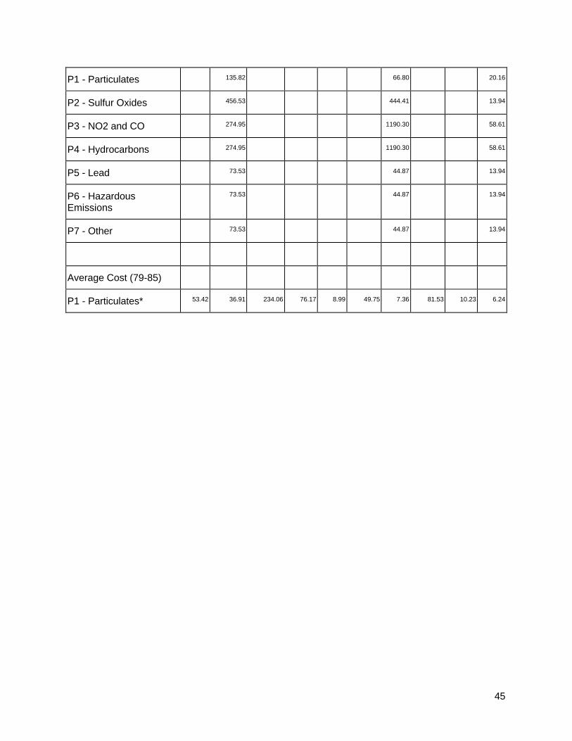
45

P1 - Particulates 135.82 66.80 20.16

P2 - Sulfur Oxides 456.53 444.41 13.94

P3 - NO2 and CO 274.95 1190.30 58.61

P4 - Hydrocarbons 274.95 1190.30 58.61

P5 - Lead 73.53 44.87 13.94


73.53 44.87 13.94

P7 - Other 73.53 44.87 13.94


P1 - Particulates* 53.42 36.91 234.06 76.17 8.99 49.75 7.36 81.53 10.23 6.24

Documents

THE COST OF AIR POLLUTION ABATEMENT - Pollution …infohouse.p2ric.org/ref/22/21765.pdf · 2002-10-22 · THE COST OF AIR POLLUTION ABATEMENT ... estimates for benefit/cost analysis