Printed: 06/02/2002 17:32 Created:16-Dec-01 09:11 Filename=CP_chap_for_DS_volume.DOC, This draft: 06/02/2002

THE CORE-PERIPHERY MODEL: KEY FEATURES

AND EFFECTS

Richard BALDWIN, Rikard FORSLID, Philippe MARTIN,

Gianmarco OTTAVIANO, AND Frédéric ROBERT-NICOUD∗

More than 25 years ago, Avinash Dixit and Joe Stiglitz developed a simple model for

addressing imperfect competition and increasing returns (ICIR) in a general equilibrium setting.

Its first application, in Dixit and Stiglitz (1977), was to an issue that now seems rather banal –

whether the free markets produces too many or too few varieties of differentiated products. But

ICIR considerations are so crucial to so many economic phenomena, and yet so difficult to

model formally, that the Dixit-Stiglitz framework has become the workhorse of many branches

of economics. In this paper, we present one of its most recent, and most startling applications –

namely, to issues of economic geography. While there are many models in this new literature,

almost all of them rely on Dixit-Stiglitz monopolistic competition, and among these, the most

famous is the so-called core-periphery model introduced by Paul Krugman in a 1991 paper.

The basic structure of the core-periphery (CP) model is astoundingly familiar to trade

economists. Take the classroom Dixit-Stigliz monopolistic-competition trade model with trade

costs, add in migration driven by real wage differences, impose a handful of normalisations, and

voila, the CP model! The fascination of the CP model stems in no small part from the fact that

these seemingly innocuous changes so unexpectedly and so radically transform the behaviour of

a model that trade theorists have been exercising for more than 25 years.

This paper presents the core-periphery model, or more precisely the version in Chapter 5

of Krugman, Fujita and Venables (1999) – FKV for short.1 We survey or describe all the main

properties of the model including catastrophe, hysteresis, and global stability.

∗ Graduate Institute of International Studies (Geneva), Stockholm University, CERAS-ENPC (Paris), Bocconi

University (Milan), and London School of Economics, respectively.

1

1. The Standard Core-Periphery Model

The basic structure of the core-periphery (CP) model assumes two initially symmetric

regions (north and south), fixed endowments of two sector-specific factors (industrial workers H

and agricultural labourers L), and two sectors (manufactures M and agriculture A). Agricultural

labourers are not geographically mobile, but industrial workers do migrate in response to the

North-South real wage differences. Trade in industrial goods is costless, so both firms and

consumers care about location.

The technology is simple. The M-sector is a standard Dixit-Stiglitz monopolistic

competition sector, where manufacturing firms (M-firms for short) employ H to produce output

subject to increasing returns. Production of each M-variety requires a fixed cost of F units of H

in addition to am units of H per unit of output, so the cost function is w(F+amx), where x is a

firm's output and w is the reward to H. The A-sector produces a homogeneous good under

perfect competition and constant returns using only L.

Both M and A are traded, with M trade is inhibited by iceberg trade costs. Specifically, it

is costless to ship M-goods to local consumers but to sell one unit in the other region, an M-firm

must ship τ≥1 units. The idea is that τ-1 units of the good “melt” in transit. As usual, τ captures

all the costs of selling to distant markets, not just transport costs, and τ-1 is the tariff-equivalent

of these costs. Importantly, trade in A is costless.2

Preferences of the representative consumer in each region has consisting of CES

preferences over M-varieties nested in a Cobb-Douglas upper-tier function that also includes

consumption of the homogenous good, A. Specifically:

(1) σµσσµµ <<<≡= ∫+

=

− 10)(; ;*

0

1 dic C CCU 1/-11

nn

i

1/-1iMAM

where CM and CA are, respectively, consumption of the M composite and consumption of A; n

and n* are the measure of north and south varieties (often we loosely refer to these as the number

1 The original model appears in Krugman (1991a,b). Venables (1996) is its vertical-linkages version. 2 Chapter 7 of FKV shows that this is an assumption of convenience in that qualitatively identical results can be

obtained in a more complex model that allows for A-sector trade costs.

2

of varieties), µ is the expenditure share on M-varieties, and σ is the constant elasticity of

substitution between M-varieties.

Migration is governed (as in FKV) by the ad hoc migration equation:

(2) σµ

σµωωω−+

=

−−

≡≡≡−−= ∫

1*

0

11,,;)1(*)(nn

iiAwHHHH dippP

Pw

HHssss

where sH is the share of world H in the north, H is the northern labour supply, Hw is the world

labour supply, ω and ω* are the northern and southern real wages, w is the northern nominal

wage for H, and P is the north’s region-specific perfect price index implied by (1); pA is the price

of A and pi is the price of M-variety i (the variety subscript is dropped were clarity permits).

Analogous definitions hold for southern variables, which are denoted with an asterisk.

1.1. Equilibrium Expressions

As is well known3, utility optimisation yields a constant division of expenditure between

M and A, and CES demand functions for M varieties, namely:

(3) LwwHEdip

Epc Lnn

i i

jj +=≡∫

+

=

−

−

;*

0

1 σ

σ µ

where E is region-specific expenditure, and wL is the wage rate of L. As usual in the Dixit-

Stiglitz monopolistic competition setting, free and instantaneous entry drives pure profits to zero,

so E involves only factor payments. Demand for A is CA=(1-µ)E/pA

On the supply side, perfect competition in the A-sector forces marginal cost pricing, i.e.

pA=aAwL and pA*=aAwL*, where aA is the unit input coefficient. Costless trade in A equalises

northern and southern prices and thus indirectly equalises L wage rates internationally, viz.

wL=wL*. In the M-sector, ‘milling pricing’ is optimal, so the ratio of the price of a northern

variety in its local and export markets is just τ. Summarising these equilibrium-pricing results:

3 Details of all calculations can be found in “All you wanted to know about Dixit-Stiglitz but were afraid to ask”,

available on http://heiwww.unige.ch/~baldwin/.

3

(4) * *, * ,1 1/ 1 1/

m mA A L

wa waLp p p p w w

τσ σ

= = = =− −

=

where p and p* are the local and export prices of a home-based M-firm. Analogous pricing rules

hold for southern M-firms.

A well known result for the Dixit-Stiglitz monopolistic competition model is that

operating profit (call this π) is the value of sales divided by σ, where the value of sales is either

shipments at producer prices, or retail sales at consumer prices.4 Using milling pricing from (4)

and the shipments-based expression for operating profit in the free entry condition, namely

px/σ=wF, yields the equilibrium firm size. This and the full employment of H – i.e. n(F+amx)=H

– yields the equilibrium number of firms, n. Specifically:

(5) maFxFHn /)1(,/ −== σσ

where x is the equilibrium size of a typical X-firm. Similar expressions define the analogous

southern variables. Two features of (5) are worth highlighting. First, the number of varieties

produced in a region is proportional to the regional labour force. H migration is therefore

tantamount to industrial delocation and vice versa. Second, the scale of firms is invariant to

everything except the elasticity of substitution and the size of fixed costs. Note also that one

measure of scale, namely the ratio of average cost to marginal cost, depends only on σ.

The market for northern X-varieties must clear at all moments and from (5) firm output is

fixed, so using (3), the market clearing condition for a typical Northern variety is5:

(6) σσ

σ

σσ

σ

φµφ

φµ

−−

−

−−

−

++

+≡= 1**1

1

1**1

1 *;wnnw

Ewwnnw

EwRRxp

4 A typical first order condition for local sales is pi(1-1/σ)=waM. Rearranging this, operating profit on local sales is

(p-waM)ci=pc/σ. A similar rearrangement of the first order condition for export sales and summation yields the result

for consumer prices. Noting that p*c*=wτc*=wτxhh/τ, where xh

h is export shipments, yields the result for producer

prices. 5 Local sales of a northern variety are w1-σ/[nw1-σ+n*(τw*)1-σ] times µE since the price of imports is τw*. The

expression for export sales is (τw)1-σ/[n(τw)1-σ+n*w*1-σ] times µE*.

4

where R is a mnemonic for ‘retail sales’. Due to markup price and iceberg trade costs, the value

of a typical firm’s retail sales at consumer prices always equals its revenue at producer prices; R

is thus also a mnemonic for revenue. Also, φ=τ1-σ measures the ‘free-ness’ (phi-ness) of trade

and note that the free-ness of trade rises from φ=0 (with infinite trade costs) to φ=1 with zero

trade costs. Equilibrium additionally requires that the equivalent of (6) for a typical southern

variety, and the market clearing condition for A hold. The latter requires:

(7) ApLEE /2*))(1( =+−µ

Eq. (6) and its southern equivalent are often called the wage equations since they can be

written in terms of w, w*, H and H*. One can make some progress by plugging (7) instead of the

southern wage equation into (6), but unfortunately there is no way to solve for the equilibrium

w’s analytically since 1-σ is a non-integer power. Numerical solutions for particular values of µ,

σ and φ are easily obtained.6

1.2. Choice of Numeraire and Units

Both intuition and tidiness are served by appropriate normalisation and choice of

numeraire. In particular, we take A as numeraire and choose units of A such aA=1. This

simplifies both the expressions for the price index and expenditure since it implies

pA=wL=wL*=1. In the M-sector, we measure M in units such that am=(1-1/σ), so that the

equilibrium prices become p=w and p*=τw, and the equilibrium firm size becomes σFx = .

The next normalisation, which concerns F, has engendered some confusion. Since we are

working with the continuum-of-varieties version of the Dixit-Stiglitz model, we can normalise F

to 1/σ.7 With this, 1=x , n=H and n*=H*. These results simplify the M-sector market-clearing

6 A MAPLE spreadsheet that shows how to solve this model numerically can be found on

http://heiwww.unige.ch/~baldwin/ 7 Since units of the sector-specific factor are also normalised elsewhere, it may seem that there is one too many

normalisations. As it turns out, the normalisation is OK in the continuum of varieties version of Dixit-Stiglitz, but

not OK in the discrete-varieties version. With a continuum of varieties, n is not, the number of varieties produced in

the north (if n is not zero, an uncountable infinity of varieties are produced in the north), it is the measure and we are

5

condition, (6). The results that n=H and n*=H* also boost intuition by making the connection

between migration and industrial delocation crystal clear.

We have not yet specified units for L or H. Choosing the world endowment of H, namely

Hw, such that Hw=1 is useful since it implies that the total number of varieties is fixed at unity

(i.e. nw=1) even though the production location of varieties is endogenous. The fact that n+n*=1

is useful in manipulating expressions. For instance, instead of writing sH for the northern share of

Hw, we could write sn or simply n. Finally, it proves convenient to have w=w*=1 in the

symmetric outcome (i.e. where n=H=1/2) and core periphery outcomes (i.e. where n=H=1 or 0).

This can be accomplished by choosing units of L such that the world endowment of the

immobile factor, i.e. Lw, equals (1-µ)/2µ.8

In summary, the equilibrium values with these normalisation are:

(8) µ

τ

/1*,*,,1**

1**,1,1,*, **

======+=+

=+=======w

nH

LLAA

EHnssHnHHnn

wnnwwwppx w p w p

where sH and sn are the north's shares of Hw and nw respectively, and, by construction, w=w*=1

in the symmetric outcome.

Note that with these normalisations the nominal wage in the core equals unity in the core-

periphery outcomes. The nominal wage in the periphery in such outcomes varies with trade

costs. Specifically, the periphery’s wage is (φµ(1+L)+µL/φ)1/σ. Of course, this is a sort of

‘virtual’ nominal wage, viz. the wage that a small group of workers would earn if they did work

in the periphery.

2. The Long Run Equilibria and Local Stability

In solving for long-run equilibria, the key variable – the state variable – is the division of

the mobile factor H between north and south.9 Inspection of the migration equation (2) reveals

free to choose the unit of this measure. In the discrete-version, n and n* are pure numbers, so this degree of freedom

is absent. 8 KFV takes Lw as µ and Aw as 1-µ, but wages are unity as long as Lw/Aw equals µ/(1-µ). 9 With our normalisation, we can write the state variable as n, H, sn or sH.

6

two types of long run equilibria. The first type – core-periphery outcomes – is where sH=1 or 0.

The second type – interior outcomes – is where ω=ω* but 0<sH<1. Given symmetry, it is plain

that ω does equal ω* when sH=1/2, so sH=1/2 is also always a long run equilibrium.10 It is

equally clear from the migration equation that when sH=1 or 0, the economy is also in

equilibrium since no migration occurs.

2.1. A Caveat on Full Agglomeration

Only one dispersion force operates in the CP model and this (local competition) becomes

very weak as trade gets very free. As a result, the model predicts that sufficiently high levels of

trade free-ness are inevitably associated with full agglomeration. The world, however, is full of

dispersion forces – comparative advantage, congestion externalities, natural resources, “real”

geography such as rivers, natural ports, etc – and these can change everything.

The point is that the model’s agglomeration forces also decrease with trade costs. This

implies that for low enough trade costs other dispersion forces that are not eroded by trade free-

ness, such as comparative advantages, will dominate the location decisions of firms with trade

becomes sufficiently free. In the literature this is called the U-shaped result. Dispersion is the

likely outcome both with trade costs are very high and when they are very low. This appealing

feature is not, unfortunately, present in the simple CP model.11

What all this means is that the core-periphery model should not be construed as

predicting that the world must end up in an agglomerated equilibrium as trade costs are lowered.

Rather the model predicts that dramatic changes in location may happen for some levels trade

costs.

Identification of these long-run equilibria, however, is only part of the analysis. Complete

analysis requires us to evaluate the local stability of these three equilibria.

10 Are there other interior steady states? Robert-Nicoud (2001) actually confirms analytically that there can also be

at most two other interior steady states. More on this below. 11 See FKV for various modifications that lead to the U-shaped result.

7

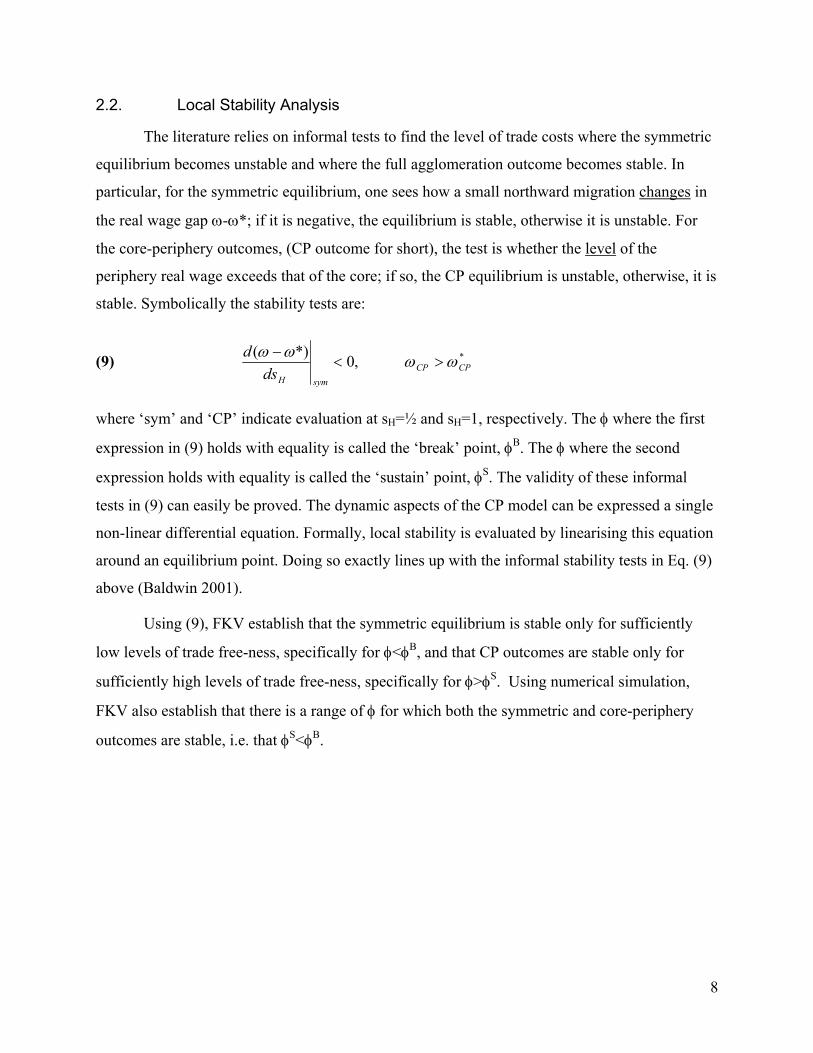
2.2. Local Stability Analysis

The literature relies on informal tests to find the level of trade costs where the symmetric

equilibrium becomes unstable and where the full agglomeration outcome becomes stable. In

particular, for the symmetric equilibrium, one sees how a small northward migration changes in

the real wage gap ω-ω*; if it is negative, the equilibrium is stable, otherwise it is unstable. For

the core-periphery outcomes, (CP outcome for short), the test is whether the level of the

periphery real wage exceeds that of the core; if so, the CP equilibrium is unstable, otherwise, it is

stable. Symbolically the stability tests are:

(9) *,0*)(CPCP

symHdsd ωωωω

><−

where ‘sym’ and ‘CP’ indicate evaluation at sH=½ and sH=1, respectively. The φ where the first

expression in (9) holds with equality is called the ‘break’ point, φB. The φ where the second

expression holds with equality is called the ‘sustain’ point, φS. The validity of these informal

tests in (9) can easily be proved. The dynamic aspects of the CP model can be expressed a single

non-linear differential equation. Formally, local stability is evaluated by linearising this equation

around an equilibrium point. Doing so exactly lines up with the informal stability tests in Eq. (9)

above (Baldwin 2001).

Using (9), FKV establish that the symmetric equilibrium is stable only for sufficiently

low levels of trade free-ness, specifically for φ<φB, and that CP outcomes are stable only for

sufficiently high levels of trade free-ness, specifically for φ>φS. Using numerical simulation,

FKV also establish that there is a range of φ for which both the symmetric and core-periphery

outcomes are stable, i.e. that φS<φB.

8

Figure 1: The Tomahawk Diagram

c

p

a

l

l

l

c

i

3

u

i

l

1

d

sH

1/2

φ0

1

1φBφS

These three facts and the long-run equilibria can be conveniently illustrated with the so-

alled ‘tomahawk’ diagram, Figure 1 (the ‘tomahawk’ moniker comes from viewing the stable-

art of the symmetric equilibrium as the handle of a double-edged axe). The diagram plots sH

gainst the free-ness of trade, φ and shows locally stable long-run equilibria with heavy solid

ines and locally unstable long-run equilibria with heavy dashed lines. Thus the three horizontal

ines sH=1, sH=1/2 and sH=0 are steady states for any permissible level of φ. Note that for most

evels of φ, there are three long-run equilibria, while for the levels of φ corresponding to bowed

urve, there are five equilibria – two core-periphery outcomes, the symmetric outcome and two

nterior, asymmetric equilibria.12

. Catastrophic Agglomeration and Locational Hysteresis

Catastrophe is the most celebrated hallmark of the CP model – probably because it is so

nexpected. Specifically, starting from a symmetric outcome and very high trade costs, marginal

ncreases in the level of trade free-ness φ has no impact on the location of industry until a critical

evel of φ is reached. Even a tiny increase in φ beyond this point causes a catastrophic

2 Of course when there is no trade cost, i.e. φ=1, distance has no meaning and the location of production is not

etermined; any division of Hw is a steady state.

9

agglomeration of industry in the sense that the only stable outcome is that of full

agglomeration.13

The key requirement for catastrophe is that the stable interior outcome becomes locally

unstable beyond a critical φ – the so-called break point – and that at the same level of trade costs,

the full agglomeration outcomes are the only stable equilibrium.

The literature traditionally uses the tomahawk diagram to illustrate the catastrophe

feature. The idea is that trade costs have, roughly speaking, fallen over time. Thus starting in the

distant past – say the pre-industrial era – trade costs were very high and economic activity was

very dispersed. As time passed, φ rose, eventually to a level beyond φB, at which point industry

rapidly became agglomerated in cities and in certain nations. Perhaps the most striking feature of

the CP model is the result that a symmetric reductions in trade costs between initially symmetric

nations eventually produces catastrophic agglomeration. That is, rising φ has no impact on the

location of industry until a critical level of openness is reached. However, even a tiny increase in

φ beyond this point results in very large location effect as the even division of industrial becomes

unstable. That non-marginal effects come from marginal changes is certainly one of the

hallmarks of the economic geography models.

The second famous feature of the CP model is hysteresis. That is, suppose we start out

with an even division of industry between the two regions and a φ between the break and sustain

points (i.e. in the so-called ‘overlap’). Given that the symmetric outcome and both full

agglomeration outcomes(core-in-the-north and core-in-the-south) are all locally stable, some

location shock, or maybe even an expectations shock, could shift industry from the symmetry

outcome to one of the core outcomes. Importantly, the locational impact would not be reversed

when the cause of the shock were removed. In other words, this model features sunk-cost

hysteresis of the type modelled by Baldwin (1988), Baldwin and Krugman (1989) and Dixit

(1989).14 The key requirement for locational hysteresis is the existence of a range of φs where

there are multiple, locally stable equilibria.

13 In the jargon, the catastrophe property is called super-critical bifurcation. 14 The feature is also sometimes called ‘path dependency’, or ‘history matters’.

10

4. The 3 Forces: Intuition for the Break and Sustain Points

The complex equilibrium structure and extremely non-neoclassical behaviour of this

model is curious, to say the least, given the fairly standard assumptions behind the model. This

section provides intuition for the complexity.

4.1. The Three Forces and the Impact of Trade Costs

There are three distinct forces governing stability in this model. Two of them—demand-

linked and cost-linked circular causality (also called backward and forward linkages) – favour

agglomeration, i.e. they are de-stabilising. The third – the local competition effect (also known as

the market crowding effect) – favours dispersion, i.e. it is stabilising.

The expressions E=wL+wAA and E*=w*(Lw-L)+wAA help illustrate the first

agglomeration force, namely demand-linked circular causality. Starting from symmetry, a small

migration from south to north would increase E and decrease E*, thus making the northern

market larger and the southern market smaller since mobile workers spend their income locally.

In the presence of trade costs, and all else being equal, firms will prefer the big market, so this

migration induced “expenditure shifting” encourages “production shifting”. Of course, firms and

industrial workers are the same thing in this model, so we see that a small migration perturbation

tends to encourage more migration via a demand-linked circular causality.

The definition of the perfect price index in (2) helps illustrate the second agglomeration

force in this model, namely cost-linked circular causality, or forward linkages. Starting from

symmetry, a small migration from south to north would increase H and thus n while decreasing

in H* and n*. Since locally produced varieties attract no trade cost, the shift in n’s would, other

things equal, lower the cost of living in the north and raise living costs in the south, thus raising

the north’s relative real wage. This in turn tends to attract more migrants.15

The lone stabilising force in the model, the so-called local competition, or market

crowding, effect, can be seen from the definition of retail sales, R, in (6). Perturbing the

symmetric equilibrium by moving a small mass of H northward, raises n and lowers n*. From

(6), we see that this tends to increase the degree of local competition in the north and thus lower

15 FKV call it the price index effect.

11

R (as long as φ<1).16 To break even, northern firms would have to pay lower nominal wages. All

else equal, this drop in w and corresponding rise in w* makes north less attractive and thus tends

to undo the initial perturbation. In other words, this is a force for dispersion of industry activity.

The catastrophic behaviour of the model stems from two facts, which we explore more

below. The first is that the dispersion force is stronger than the agglomeration forces at high

trade costs. The second is that raising the level of trade free-ness reduces the magnitude of each

of the three forces, but it erodes the strength of the dispersion force faster. As a result, at some

level of trade costs – the break point – the agglomeration forces become stronger than the

dispersion force and industry collapses into just one region. For readers who wish to understand

these forces in more depth, we turn now to a series of thought experiments that more precisely

illustrate the forces and their dependence on trade costs.

4.2. A Series of Thought Experiments

Focusing on each of the three forces separately boosts intuition and we accomplish this

via a series of thought experiments. These focus on the symmetric equilibrium for a very

pragmatic reason. In general, the CP model is astoundingly difficult to manipulate since the

nominal wages are determined by equations that cannot be solved analytically. At the symmetric

equilibrium, however, this difficulty is much attenuated. Due to the symmetry, all effects are

equal and opposite. For instance, if a migration shock raises the northern wage, then it lowers the

southern wage by the same amount. Moreover, at the symmetric outcome, w=w*=1, so much of

the intractability – which stems largely from terms involving a nominal wage raised to a non-

integer power –disappears.

The Local Competition Effect

To separate the production shifting and expenditure shifting aspects of migration, the first

thought experiment supposes that H migration is driven by nominal wages differences and that

16 In Dixi-Stiglitz competition, the price-cost mark-up never changes, so this local competition effect is not a pro-

competitive effect. This is why some authors prefer the term “market crowding”.

12

all H earnings are remitted to the country of origin.17 Thus, migration changes n and n* but not E

and E*.

Log differentiating (6) yields (using “^” to indicate proportional change):

(10) )ˆˆ)(2/1(2ˆ

*);ˆ*)(1()ˆˆ(ˆ

2/1

1

∆−−=∆

≡∆−−+∆−=

=

−

ERs

RERER

ssw

nwsssssw

nσ

σσ

where ∆=nw1-σ+φn*w*1-σ, ∆*=φnw1-σ+n*w*1-σ, sR is share of a typical north firm’s total sales, R,

that are made in the north and the second expression follows due to the equal and opposite nature

of all changes around symmetry; all share variables such as sR, sE and sn lie in the zero-one

range. Observe that at the symmetric outcome (i.e. sn=sH=½), sR exceeds ½ when trade is not

perfectly free, i.e. φ<1. Moreover, sR falls toward ½ as φ approaches unity; specifically,

sR=1/(1+φ) at sH=½.

By supposition, expenditure is repatriated so 0ˆ =Es , and given the definition of ∆:

(11) )ˆ)1(ˆ)(2/1(2ˆ2/1 wnsMsn

−−−=∆ = σ

where sM is the share of northern expenditure that falls on northern M-varieties. With positive

trade costs, sM exceeds ½ with the difference shrinking as φ increases; in fact using the demand

functions and symmetry we can show that 2(sM-½)=(1-φ)/(1+φ). Using (11) in (10) with dsE=0

yields:

(12) nss

sswMR

MR ˆ)1)(2/1)(2/1(4

)2/1)(2/1(4ˆ−−−−

−−−=

σσ

This is the “local competition” effect in isolation. Note that sR and sM lie in the zero-one range.

There are four salient points. First, since the denominator must be positive (since 4(sR-

½)(sM-½) is always less than unity and σ>1) and the numerator must be negative, northward

17 This may be thought of as corresponding to the case where H is physical capital whose owners are immobile. Note

also that under these suppositions, the model closely resembles the pre-economic geography models with

monopolistic competition and trade costs, e.g. Venables (1987) and Chapter 10 of Helpman and Krugman (1985).

13

migration always lowers the northern nominal wage and, by symmetry, raises the southern wage.

Second, this shows directly that migration is not, per se, destabilising. When the demand or cost

linkages are cut, as in this thought experiment, the symmetric equilibrium is always stable

despite migration. Third, the magnitude of this “competition for consumers” effect diminishes

roughly with the square of trade costs since as trade free-ness rises, (sR-½) and (sM-½) fall.

Specifically, 4(sR-½)(sM-½)=[(1-φ)/(1+φ)]2. Note that in FKV terminology (sR-½) and (sM-½) are

denoted as “Z” since at the symmetric equilibrium both equal (1-φ)/(1+φ).

The final point is that in this thought experiment the break and sustain points are

identical; this can be seen by noting that sn doesn't enter (12). Both points equal φ=1 since the

symmetric outcome is stable, and the core-periphery outcome is unstable for any positive level of

trade costs. When there are no trade costs, any locational outcome is an equlibirum.

Demand Linkages

In the next thought experiment, suppose that, for some reason, H bases its migration

decision on nominal wages but spends all of its income in the region it is employed. While this

would not make much sense to a rational H-worker, the assumption serves intuition by allowing

us to restore the connection between production shifting (dH=dn) and expenditure shifting dE

without at the same time adding in the cost-linkage (i.e. cost-of-living effect). Since E equals

L+wH and this equals L+wn with our normalisations, the restored term from (10) is:

(13) )ˆˆ()ˆˆ(ˆ nwnwE

wnsE +=+= µ

The second expression follows since, from (8), w=1, n=½ and E=1/2µ at the symmetric outcome.

Using (13) and (11) in (10), we find:

(14) µσσ

µ−−−−−−−−−

== )1)(2/1)(2/1(4ˆ)2/1)(2/1(4ˆ)2/1(2ˆ 2/1

MR

MRRs ss

nssnswn

Note that the denominator is always positive, since 0≤4(sR-½)(sM-½)≤1.

Six aspects of (14) are worth highlighting. First, the de-stabilising aspects of demand-

linked circular causality can be seen by the fact that the first term in the numerator is positive.

Second, the size of the de-stabilising demand linkage increases with the M-sector expenditure

14

share, µ. This makes sense since as µ rises, a given amount of expenditure shifting has a bigger

impact on the profitability of locating in the north. Third, the size of this destabilising effect falls

as trade gets freer since sR approaches ½ as φ approaches unity. Fourth, the magnitude of the

stabilising local-competition effect erodes faster than the de-stabilising force since both sR and sM

approach ½ as φ approaches unity. Fifth, the symmetric outcome is stable with very high trade

costs. To see this observe that 4(sR-½)(sM-½)=2(sR-½)=1 at φ=0 and µ<1.Finally, at some level

of trade free-ness, namely φb’=(1-µ)/(1+µ), dw/dn is zero. This critical value is useful in

characterising the strength of agglomeration forces since it defines the range of trade costs where

agglomeration forces outweigh the dispersion force. Thus an expansion of this range (i.e. a fall in

the critical value) indicates that agglomeration dominates over a wider range of trade costs.

Cost-of-Living Linkages

The above thought experiments isolate the importance of the local competition effect and

demand-linked circular causality. The final force operating in the model works through the cost-

of-living effect. Since the price of imported varieties bears the trade costs, consumers gain –

other things equal – from local production of a variety. This effect, which we dub the “location

effect”, is a de-stabilising force. A northward migration shock leads to production shifting that

lowers the cost-of-living in the north and thus tends to makes northward migration more

attractive. To see this more directly, we return to the full model with H basing its migration

decisions on real wages and spending their incomes locally. Log differentiating the northern real

wage, we have . Using (11): )1/(ˆˆˆ σµϖ −∆−= w

(15) nssw RRsnˆ)2/1(2

1))2/1(21(ˆˆ 2/1 −

−+−−== σ

µµω

The second term is the cost-of-living effect, also known as cost-linked circular causality, cost

linkages, or backward linkages. Since this is positive, the cost-of-living linkage is de-stabilising

in the sense that it tends to make more positive the real wage change stemming from a given

migration shock. Moreover, consumers care more about local production as µ/(σ-1) increases, so

the magnitude of the cost-of-living effect increases as µ rises and σ falls. Higher trade costs also

amplify the size of the effect since sR rises towards 1 as φ approaches zero.

15

Two observations are in order. Observe first that the cost-linkage can be separated

entirely from the demand and local competition effects. The first term in (15) captures the

demand-linkage and the local competition effect, while the second term captures the cost-

linkage. Second, note that the coefficient on is positive – since 2(sw R-½)≤1 – so the net impact

of the demand linkage and local competition effects on ω depends only on the sign of (14).

The No-Black-Hole Condition

To explore stability at very high trade costs, we use (14) and set φ=0 to get thatϖ at sn=½

equals )1/(ˆˆ)1( σµµ −+−− nn . Stability requires this to be negative and solving we see that this

holds only when µ<(1-1/σ). If this, which FKV call the ‘no black hole’ condition, holds, then the

dispersed equilibrium is stable with very high trade costs. Otherwise, the symmetric equilibrium

is never stable.

4.3. The Break Point

We have seen that the magnitude of both the agglomeration and dispersion forces

diminish as trade cost fall, but the dispersion force diminishes faster than the agglomeration

forces. We also saw that when the no black hole condition holds, the symmetric equilibrium is

stable – i.e. the dispersion force is stronger than the agglomeration forces – for very high trade

costs.

Figure 2 illustrates both of these facts. The bifurcation point (i.e. the level of trade costs

where the nature of the model’s stability changes) is where the agglomeration and dispersion

forces are equally strong.

Finally, noting that 2(sR-½)=2(sM-½)=(1-φ)/(1+φ), we can find the level of φ where the

bifurcation occurs by plugging (14) into (15), setting the result equal to zero and solving for φ.

The solution is:

(16) )11(

1)1(1)1(

µµ

µσµσφ

+−

−+−−

=B

The break point can be used as a metric for the relative strength of agglomeration forces.

For example, if a particular parameter change reduces φB, it must be that the change leads the

16

agglomeration forces to overpower the dispersion force at a higher level of trade costs. This, in

turn, implies that the change has strengthened the agglomeration forces relative to the dispersion

forces.

F

m

w

l

f

t

4

r

φ

Magnitude of forces

1

Dispersion Forces (local competition effect)

Agglomeration Forces(backward & forward linkages)

Bifurcation

φbreak

igure 2: Agglomeration and Dispersion Forces Erode with φ

Note that from (16), the break point falls when µ rises and when σ falls. This should

ake sense since µ magnifies both the demand-linked and the cost-linked agglomeration forces,

hile a fall in the substitutability of varieties, i.e. a rise in 1/(σ-1), magnifies the cost-of-living

inked agglomeration (by strengthening the utility benefit of local production). Of course, with

ree entry, 1/σ is also a measure of scale (see Appendix 1), so, loosely speaking, we can also say

hat an increase in equilibrium scale economies magnifies the cost-of-living agglomeration force.

.4. The Sustain Point

The sustain point is much easier to characterise since it involves the comparison of levels

ather than the signing of a derivative. Specifically, we evaluate w/P and w*/P* at the CP

17

outcome (we take sn=sH=1, although sn=sH=0 would do just as well) and look for the level of φ

where the two real wages are equal. Given our normalisation, w and P equal unity at the CP

outcome (to see this plug n=1 and n*=0 into (6) to find w=1 and then use this and n=1 and n*=0

in the definition of P). Using the southern equivalent of (6), we have (w*)σ=φµ(1+L)+µL/φ) at

the CP outcome, where L is each region’s endowment of the immobile factor and L=(1-µ)/2µ

with our normalisations. Plainly, this w* is a sort of ‘virtual’ nominal wage since no labour is

actually employed in the south when sH=1. Finally, in the south all M-varieties are imported

when sH=1, so P*=φµ/(1-σ). Putting these points together, the sustain point is implicitly defined by:

(0.17) µµ

φφµµφ

σµ

σ

21;

)()/)1((

**1 1/

/1 −=

++=== − LLL

Pw

Pw

S

SS

With some manipulation, this can be shown to be equivalent to the following implicit definition

for the sustain point:

(18) ( ) ( )1 21 1/ 1 11

2 2S S

µσ µ µφ φ−

− + − = +

4.5. Tomahawk bifurcation

The bifurcation diagram has the shape a tomahawk, as Figure 1 shows. This means that

the sustain point occurs at a lower level of trade free-ness than the break point and that there are

at most three interior steady-states at all levels of trade free-ness short of full integration, namely

for all φ in [0,1). We now turn to these issues.

Comparing the Break and Sustain Points

The fact that the sustain point occurs at a lower level of trade free-ness than the break

point is well known and has been demonstrated in thousands of numerical simulations by dozens

of authors. Yet a valid proof of this critical feature of the model was never undertaken until

recently.18

18 The first draft of the excellent paper by Peter Neary (2001), was seen by us before we wrote this chapter. That

draft contained a brief proof in a footnote that turned out to be incorrect. One of the authors showed the proof’s error

18

1RHS

F

m

d

t

e

w

n

b

f

a

µ

a

S

-0.6

-0.4

-0.2

0

0.2

0.4

0.6

0.8

0 0.2 0.4 0.6 0.8 1φ

f(φΒ)

φΒ

12

12

1)( 21

/11 −

−

++

=−

− µφµφφ σµ

f

φS

igure 3: Proving the φB>φS.

The most satisfying approach to proving that φS<φB would be direct algebraic

anipulation of expressions for the two critical points. This is not possible since φS can only be

efined implicitly as in (0.17). Instead, we pursue a two-step proof. First we characterise the how

he function, 1]2/)1()1[()( 21

/11 −−++=−

− µφµφφ σµ

f , this is just a transformation of the second

xpression in (0.17), changes with φ. This function is of interest since φS is its root. With some

ork we can show three facts: that f(1)=0 and f’(1) is positive, that f(0) is positive and f’(0) is

egative, and that f(.) has a unique minimum. Taken together, this means f has a unique root

etween zero and unity. In short, it looks like the f drawn in Figure 3. Next, we show that

(φB)<0, which is only possible if φS<φB, given the shape of f(.). To this end, observe that f(φB) is

function of µ and σ. Call this new function g(µ,σ) and note that the partial of g with respect to

is negative and g(0,σ) is zero regardless of σ. The point of all this is that the upper bound of g,

nd provided a correct proof, which Peter Neary incorporated (with accreditation) in subsequent drafts of his paper.

ee also Robert-Nicoud (2001).

19

and thus the upper bound of f(φB), is zero. We know, therefore, that for permissible values of µ

and σ, φS>φB.

On the Number of Interior Steady States

Until recently, no analytical study supported the tomahawk configuration of the

bifurcation diagram: thousands of simulations showed that when there were asymmetric interior

steady-states they featured the following characteristics. First, they always come in symmetric

pairs (this is hardly surprising given the symmetry of the model), namely, if some sH different to

½ is a solution to Ω[sH]=0, then 1-sH is a solution, too. Second, these asymmetric steady-states

are always unstable: dΩ/d sH is positive for all sH>½ such that Ω[sH]=0. Finally, there are at most

two of them.

To show this result, it is sufficient to invoke the result in section 4.5 above and that

Ω[.]=0 admits at most three solutions. See Figure 1 to get convinced. The proof for this result

involves essentially two steps. The first step is to rewrite the model in its ‘natural’ state space,

namely the mobile nominal expenditure sHw rather than the mass of mobile workers sH. To this

end, it is useful to note that the Cobb-Douglas specification for tastes in (1) implies sHw+(1-

sH)w*=1, hence sHw is the share of mobile expenditure spent in North. The second step is to

show that the alternative core-periphery model developed by Forslid and Ottaviano (2001) is

identical to the original version surveyed here when expressed in the same, natural, state space.

Since this model is known to admit at most three interior steady-states, the same must be true for

the original core-periphery model analysed here. This methodology extends to geography models

in which agglomeration is driven by input-output linkages (FKV, chapter 14). See Robert-

Nicoud (2001) for details.

5. Caveats

5.1. When Does Symmetry Break? Pareto Dominance and Migration Shocks

The analysis to this point has focused only on local stability, as is true of the vast

majority of the literature. This is not enough. For instance, when does symmetry would break as

trade costs fell gradually from prohibitive to negligible? The standard answer is that it breaks at

the break point. This is not necessarily true. For levels of trade free-ness between φS and φB,

20

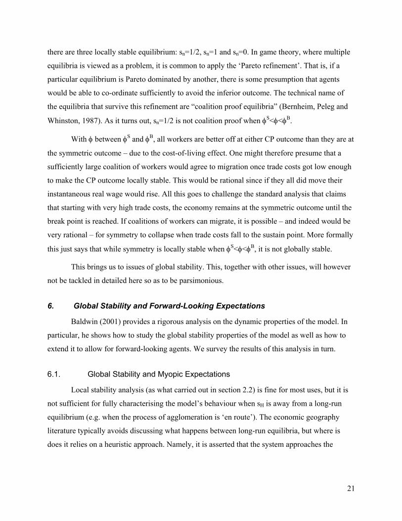
there are three locally stable equilibrium: sn=1/2, sn=1 and sn=0. In game theory, where multiple

equilibria is viewed as a problem, it is common to apply the ‘Pareto refinement’. That is, if a

particular equilibrium is Pareto dominated by another, there is some presumption that agents

would be able to co-ordinate sufficiently to avoid the inferior outcome. The technical name of

the equilibria that survive this refinement are “coalition proof equilibria” (Bernheim, Peleg and

Whinston, 1987). As it turns out, sn=1/2 is not coalition proof when φS<φ<φB.

With φ between φS and φB, all workers are better off at either CP outcome than they are at

the symmetric outcome – due to the cost-of-living effect. One might therefore presume that a

sufficiently large coalition of workers would agree to migration once trade costs got low enough

to make the CP outcome locally stable. This would be rational since if they all did move their

instantaneous real wage would rise. All this goes to challenge the standard analysis that claims

that starting with very high trade costs, the economy remains at the symmetric outcome until the

break point is reached. If coalitions of workers can migrate, it is possible – and indeed would be

very rational – for symmetry to collapse when trade costs fall to the sustain point. More formally

this just says that while symmetry is locally stable when φS<φ<φB, it is not globally stable.

This brings us to issues of global stability. This, together with other issues, will however

not be tackled in detailed here so as to be parsimonious.

6. Global Stability and Forward-Looking Expectations

Baldwin (2001) provides a rigorous analysis on the dynamic properties of the model. In

particular, he shows how to study the global stability properties of the model as well as how to

extend it to allow for forward-looking agents. We survey the results of this analysis in turn.

6.1. Global Stability and Myopic Expectations

Local stability analysis (as what carried out in section 2.2) is fine for most uses, but it is

not sufficient for fully characterising the model’s behaviour when sH is away from a long-run

equilibrium (e.g. when the process of agglomeration is ‘en route’). The economic geography

literature typically avoids discussing what happens between long-run equilibria, but where is

does it relies on a heuristic approach. Namely, it is asserted that the system approaches the

21

nearest stable equilibrium that does not require crossing an unstable equilibrium. Baldwin (2001)

uses Liaponov’s direct method to show that this heuristic approach can be justified formally.

6.2. Local Stability and Forward-Looking Expectations

Perhaps the least attractive of the CP-model assumptions concerns migrant behaviour.

Migrants are assumed to ignore the future, basing their migration choices on current real wage

differences alone. This is awkward since migration is the key to agglomeration, workers are

infinitely lived, and migration alters wages in a predictable manner. While the shortcomings of

myopia were abundantly clear to the model’s progenitors, the assumption was thought necessary

for tractability. This turns out not to be true. The first thing to note is that myopic behaviour is

tantamount to static expectations. Also, an important and somewhat unexpected result is that the

break and sustain points are exactly the same with static and with forward-looking expectations.

In this sense, the law of motion in (2) is merely an assumption of convenience.

6.3. Global Stability and Forward-Looking Expectations

When trade costs are such that the CP model has a unique stable equilibrium, local

stability analysis is sufficient. After any shock, the asset value of migration (a co-state variable)

jumps to put the system on the saddle path leading to the unique stable equilibrium (if it did not,

the system would diverge and thereby violate a necessary condition for intertemporal

optimisation). For φ’s where the model has multiple stable steady states things are more

complex. With multiple stable equilibria, there will be multiple saddle paths. In principle,

multiple saddle paths may correspond to a given initial condition, thus creating what Matsuyama

(1991) calls an indeterminacy of the equilibrium path. In other words, it is not clear which path

the system will jump to, so the interesting possibility of self-fulfilling prophecies and sudden

takeoffs may arise.

Assume φS<φ<φB throughout so that the system is marked by three stable steady states.

Three qualitatively different cases are consider for the migration cost parameter γ . The first case

is when γ, the migration cost parameter, is very large, so horizontal movement is very slow.

Numerical simulations show there is no overlap of saddle paths in this case, so the global

stability analysis with static expectations is exactly right. That is, the basins of attraction for the

various equilibria are the same with static and forward-looking expectations. This is an important

22

result. It says that if migration costs are sufficiently high, the global as well as the local stability

properties of the CP model with forward-looking expectations are qualitatively identical those of

the model with myopic migrants.

The second case is for an intermediate value of migration costs. Here the saddle paths

overlap somewhat. The existence of overlapping saddle paths changes things dramatically, as

Krugman (1991c) showed. If the economy finds itself with a level of sn that lays in the overlap,

then a fundamental indeterminacy exists. Both saddle paths provide perfectly rational adjustment

tracks. Workers individually choose a migration strategy taking as given their beliefs about the

aggregate path. Consistency requires that beliefs are rational on any equilibrium path. That is, the

aggregate path that results from each worker’s choice is the one that each of them believes to be

the equilibrium path. Putting it more colloquially, workers chose the path that they think other

workers will take. In other words, expectations, rather than history, can matter.

Because expectations can change suddenly, even with no change in environmental

parameters, the system is subject to sudden and seemingly unpredictable takeoffs and/or

reversals. Moreover, the government may influence the state of the economy by announcing a

policy, say a tax, that deletes an equilibrium even when the current state of the economy is

distant to the deleted equilibrium.

The final case is the most spectacular. Here migration costs are very low, so horizontal

movement is quite fast. Interestingly, the overlap of saddle paths includes the symmetric

equilibrium. This raises the possibility that the economy could jump from the symmetric

equilibrium onto a path that leads it to a CP outcome merely because all the workers expected

that everyone else was going to migrate. Plainly, this raises the possibility of a big-push drive by

a government having some very dramatic effects.

We conclude with two remarks. First, note that the region of overlapping saddle paths

will never include a CP outcome. Thus, although one may ‘talk the economy’ out of a symmetric

equilibrium, one can never do the same for an economy that is already agglomerated. Finally,

Karp (2000) assumes that agents have ‘almost common knowledge’ in the sense of Rubinstein

(1989) about history (economic fundamentals) rather than common knowledge. In a setting akin

to Matsuyama (1991) and Krugman (1991c), he shows that the equilibrium indeterminacy

brought about by the possibility that expectations might prevail above history washes away.

23

Common knowledge and rational expectations together give rise to the possibility that

expectations might prevail over history in the first place, so it is not surprising that altering the

information structure alters the equilibrium set considerably. We conjecture that the same holds

true in the present Core-Periphery model with forward-looking expectations. As Karp (2000)

points out, the restoration of the determinacy implies that ‘the unique competitive equilibrium

can be influenced by government policy, just as in the standard models.’

7. Concluding remarks

In ending, we can do no better than to quote an early draft of Peter Neary’s Journal of

Economic Literature article on the new economic geography literature.

“’New economic geography’ has come of age. Launched by Paul Krugman in a 1991

Journal of Political Economy paper; extended in a series of articles by Krugman, Masahisa

Fujita, Tony Venables and a growing band of associates; soon to be institutionalised with the

appearance of a new journal; it has now been consolidated and comprehensively synthesised

in a recent book from MIT Press.

Such rapid progress would make anyone dizzy, and at times the authors risk getting carried

away by their heady prose style. Thus, the structure of equilibria predicted by one model

suggests a story which they call (following Krugman and Venables (1995)) ‘History of the

World, Part I’ (page 253); the pattern of world industrialisation suggested by another is

described as "a story of breathtaking scope" (page 277); and on his website Krugman

expresses the hope that economic geography will one day become as important a field as

international trade. This sort of hype, even if tongue-in-cheek, is not to everyone's taste,

especially when the results rely on special functional forms and all too often can only be

derived by numerical methods. What next, the unconvinced reader may be tempted to ask?

the tee-shirt? the movie?”

This reaction is even more remarkable when one notes that the basic elements of the

model have been in circulation since Dixit and Stiglitz (1977) and Krugman (1980). In this

paper, we propose an exhaustive presentation of the core-periphery model, decomposing the

effects at work so as to boost intuition. We have described all the main properties of the model

24

(using analytical analysis rather than simulations whenever it was possible), including

catastrophe, hysteresis, the number of steady states, and global stability. For lack of space, we

were content with merely mentioning some of them, especially the most technical ones. Baldwin

et al. (2001) cover these properties in depth and also consider the case of intrinsically

asymmetric regions.

REFERENCES

Baldwin, R. E. (1993): “Hysteresis in Import Prices: The Beachhead Effect,” American

Economic Review 78(4) 773-85

Baldwin, R.E. (2001): "The core-periphery model with forward-looking expectations," Regional

Science and Urban economics 31: 21-49.

Baldwin, R.E., R. Forslid, P. Martin, G.I.P. Ottaviano, and F. Robert-Nicoud (2001). Economic

Geography and Public Policies, Manuscript.

Baldwin, R. E. and P. Krugman (1989): “Persistent Trade Effects of Large Exchange Rate

Shocks,” Quarterly Journal of Economics 104(4), 635-54

Bernheim, B.D., B. Peleg, and M. D. Whinston (1987). "Coalition-Proof Nash Equilibria I:

Concepts," Journal of Economic Theory, 42, 1-12.

Davis, D. (1998): "The home market, trade and industrial structure," American Economic Review,

88:5, 1264-1276.

Dixit, A.K. (1989): “Hysteresis, Import Penetration, and Exchange Rate Pass-Through,”

Quarterly Journal of Economics 104(2) 205-28.

Dixit, A.K. and J.E. Stiglitz (1977): "Monopolistic competition and optimum product diversity,"

American Economic Review, 67, 297-308.

Flam, H. and E. Helpman (1987). “Industrial policy under monopolistic competition.” Journal of

International Economics 22: 79-102.

Forslid, R. and G. Ottaviano (2001): “Trade and agglomeration: Two analytically solvable

cases,” Mimeo, Lund University.

25

Fujita M., Krugman P. and A. Venables, (1999): The Spatial Economy: Cities, Regions and

International Trade, MIT Press.

Helpman, E. and P.R. Krugman (1985): Market Structure and Foreign Trade, Cambridge, Mass.:

MIT Press.

Karp, Larry (2000): “Fundamentals versus beliefs under almost common knowledge,” Mimeo,

UC Berkeley.

Krugman P. (1991a): “Increasing Returns and Economic Geography”, Journal of Political

Economy, 99, 483-99.

Krugman P. (1991b): Geography and Trade, MIT Press.

Krugman P. (1991c): “History versus Expectations,” Quarterly Journal of Economics, 106, 2,

651-667.

Krugman, P.R. and A.J. Venables (1995): "Globalization and the inequality of nations," Quarterly

Journal of Economics, 110:4, 857-880.

Matsuyama, K. (1991): “Increasing returns, industrialization and indeterminacy of equilibrium,”

Quarterly Journal of Economics 106(2): 617-650.

Neary, J.P. (2001): “Of hype and hyperbolas: Introducing the new economic geography,” Journal of

Economic Literature, 39: 536-61.

Puga, D. (1999): ''The rise and fall of regional inequalities,'' European Economic Review 43:

303-34.

Robert-Nicoud, F. (2001): “The structure of standard models of the New Economic Geography,”

Mimeo, LSE.

Rubinstein, Ariel (1989): “The electronic email game: Strategic behaviour under almost common

knowledge,” American Economic Review, 79, 385-91.

Venables, A. (1987): “Trade and trade policy with differentiated products: A Chamberlinian-

Ricardian model,” Economic Journal, 97, 700-717.

Venables, A.J. (1996): "Equilibrium locations of vertically linked industries," International

Economic Review, 37, 341-359.

26