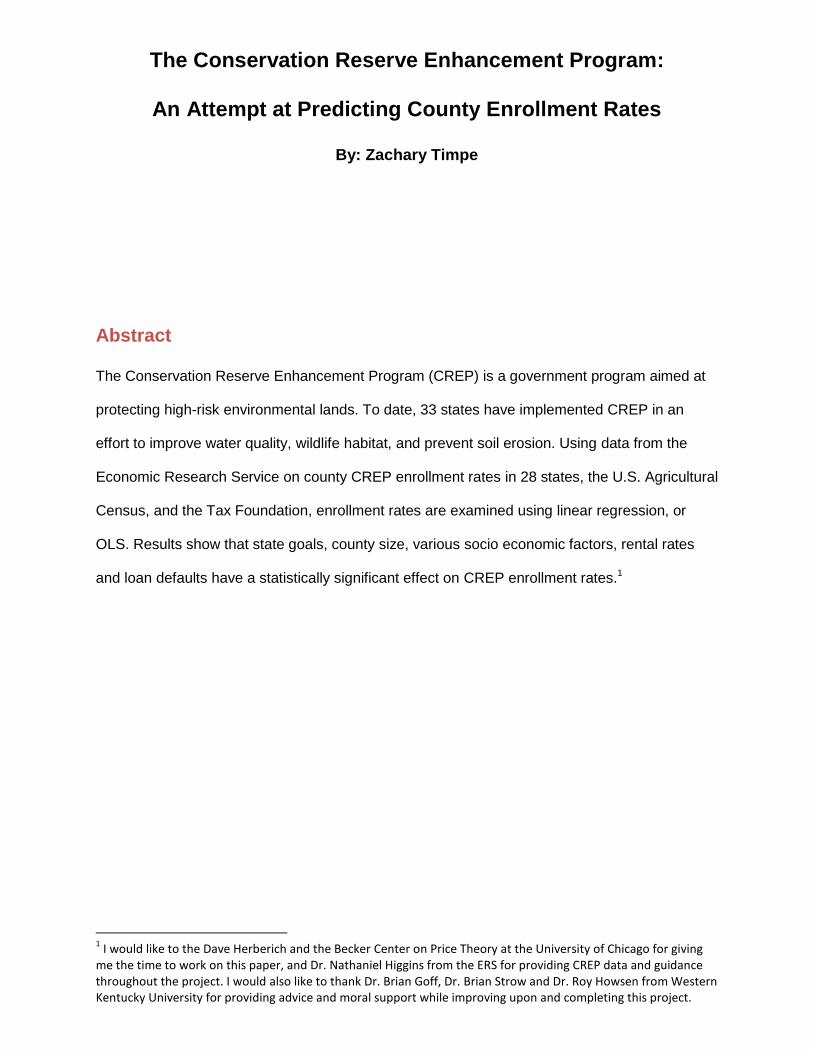
The Conservation Reserve Enhancement Program:

An Attempt at Predicting County Enrollment Rates

By: Zachary Timpe

Abstract

The Conservation Reserve Enhancement Program (CREP) is a government program aimed at

protecting high-risk environmental lands. To date, 33 states have implemented CREP in an

effort to improve water quality, wildlife habitat, and prevent soil erosion. Using data from the

Economic Research Service on county CREP enrollment rates in 28 states, the U.S. Agricultural

Census, and the Tax Foundation, enrollment rates are examined using linear regression, or

OLS. Results show that state goals, county size, various socio economic factors, rental rates

and loan defaults have a statistically significant effect on CREP enrollment rates.1

1 I would like to the Dave Herberich and the Becker Center on Price Theory at the University of Chicago for giving

me the time to work on this paper, and Dr. Nathaniel Higgins from the ERS for providing CREP data and guidance throughout the project. I would also like to thank Dr. Brian Goff, Dr. Brian Strow and Dr. Roy Howsen from Western Kentucky University for providing advice and moral support while improving upon and completing this project.

Introduction

Governmental intervention in agriculture markets to protect environmental

concerns and improve environmental performance has been cost-effective and

beneficial to the public (Claasen, Cattaneo, & Johnasson, 2008). One such program

aimed at improving environmental health is the Conservation Reserve Enhancement

Program (CREP), created in 1996 under the Farm Bill (Farm Bill). An extension of the

Conservation Reserve Program (CRP), which was adopted through the 1985 Farm Bill,

CREP’s objective is to help “agricultural producers protect environmentally sensitive

land, decrease erosion, restore wildlife habitat, and safeguard ground and surface

water” (usda.gov/crep). That is, CREP provides agricultural producers incentives to

protect natural resources on the farm which can in turn benefit the community.

CREP focuses on high-priority conservation issues at both the local and national

level, and only certain counties are eligible for help. Contracts of both the CRP and

CREP require 10- to 15-year agreements to cease agricultural production. The

compensation for this includes payment from the federal government at a

predetermined rate, an incentive payment, cost-share of up to 50% of the costs of

installing the practice, and most participants are offered a sign-up incentive to install

specific practices. Benefits from this program are many. They include: wildlife habitat

restoration, increased water quality, conservation of soil, carbon sequestration and

wetlands restoration, amongst others. Farmers who enroll land in CREP are also paid

higher rates than those who enroll in CRP, primarily because CREP has stricter

requirements for eligible land and conservation practices and looks to enroll high danger

environmental areas. Lastly, farmers can enroll at any time in CREP, whereas some

CRP programs require enrollment at specific times. Recently, CRP has opened up to

continuous enrollment, but in the past this was not available. Not all states have

adopted CREP but to date, 33 states employ CREP. CREP funding and participation

depends on each state and county’s environmental concern, with each area determining

a goal amount of land to protect. This study uses county level data from 28 states to

examine incentives to enroll. For a look at state level statistics, please refer to table 4.

Delaware, Vermont, New York and Arkansas were dropped from the dataset because of

issues with determining the state’s total goal enrollment. Hawaii and Georgia were not

included with the original dataset either because of the lack of statistics for these two

new programs.

A Review of CREP Literature

Three types of incentives are usually offered to entice enrollment in CREP, no

matter the state. Cost sharing by Federal and state governments, USDA annual base

rental payments to offset opportunity costs of idling acreage, and an up-front payment

have been offered across almost all states (Smith, 2000). Smith found that for the first

four years of the study enrollment progress was slow, citing the need for a broader

definition of eligible land, suspension of enrollment due to depleted funds, and the need

for staff or funds to market CREP. It also found that some farmers wait to enroll when

knowledge of upcoming increases in incentives are present. Nevertheless, since 2000

enrollment and participation has increased from 13 to 33 states. Allen (2005) also

evaluated the progress of CREP over the first decade of existence. Signs of

improvement come to light. Bird surveys in 2001 and 2002 found that avian species

tended to dwell more densely on management properties (i.e. CREP) than control

routes (Wisconsin Department of Agriculture, Trade and Consumer Protection 2004).

Allen cited Wentworth and Brittingham (2003) finding that CREP fields 40 acres and

larger were more likely to contain grassland birds than smaller fields. It also cited Davie

& Lant (1994), Lee et al (1999) and Mersie et al (2003), finding that water quality can

take decades to measure, and is effected by soil and sediment characteristics, weather

events, vegetative characteristics, and quality of conservation practices. But there are

still signs of improvement within water quality. Minnesota estimated that CREP reduced

sediments by 9.6 tons/acre/year (Lines 2003). North Carolina estimates CREP helped

to reduce sedimentation by 26,510 tons/year (State of North Carolina 2004a). And in

Wisconsin 1,015 miles of buffers have been established on streams and shorelines,

which has been credited with decreased annual phosphorus input by 106,000 lbs and

nitrogen input by 55,000 lbs.

Because CREP was adopted in 1996, acreage enrolled is just now becoming

eligible for reenrollment. Economists and politicians are interested to learn which

incentives create efficient and meaningful enrollment. Reenrollment data in CREP is

essentially non-existent because of the young age of the program coupled with the

length of contracts (typically 15 years). However, there is a small amount of literature

looking at CREP’s enrollment throughout the first decade and a relatively vast body

analyzing CRP.

Bills, Poe, and Suter (2008) is a novel approach aimed at measuring landowners’

responsiveness to incentives. Using the tobit method to evaluate enrollment data from

CREP and Geographic Information Systems (GIS) to estimate the amount of land

eligible for CP(22) conservation (riparian buffer acreage), the study confirms that

landowners are positively and significantly responsive to payment incentives, and

shows that the most efficient means to meeting conservation goals is to enhance

incentives offered at the beginning of the contract period rather than throughout the

contract. That is, increase upfront bonus incentives. As the paper stipulates, previous

studies using actual enrollment data from CRP have potential for bias because

participants are the only subjects. Rather, acreage not enrolled should be accounted

for to gauge for disparities in participation rates and to attempt to measure Willingness-

to-Participate (WTP).

Parks and Schorr (1997) uses actual enrollment data from CRP to analyze

agricultural producer’s decisions whether to participate in conservation programs,

continue farming as in the past, or sell the land. It found that conservation programs are

of little value to producers in densely populated areas (metropolitan counties). Policy

makers should focus on combating opportunity costs associated with non-farm uses in

densely populated areas (i.e. land development rights). Incentive responsiveness was

perceived through the discounted value of a 10-year series of payments in the amount

of the county’s maximum allowable rental rate. Hardie, Lynch, and Parker (2002) also

examine the financial incentives which induce Maryland farmers to install riparian

buffers. They develop a random utility model taking the incentive payment for buffer

installation into account and find that higher incentive payments, part-time farming, and

education positively influence the individual’s willingness to install a riparian buffer.

Other studies have used hypothetical survey data to determine incentives and

factors that affect an individual’s decision to enroll with a program such as the CRP or

CREP (i.e. Lohr and Park 1995 and Cooper and Osborn 1998). Cooper and Osborn

(1998) surveyed subjects already enrolled through CRP for willingness to re-enroll, and

find that an increase in rental payment from $30 to $85 would increase renewal from 30

to 85%. It deduced that 50% of participants would be willing to re-enroll for less than

the current rental rate, while an achievement of nearly 100% of eligible land would

require drastically higher rental rates. Lohr and Park (1995) used Contingent Valuation

(CV) survey data to estimate the probability of enrolling in a conservation program. CV

surveys are used to create probability of participation in voluntary soil conservation

programs, but they don’t show a real decision making process because an individual

must first make a discrete choice (do I enroll in program or not?) and then make a

continuous decision on the rate of participation (how much of eligible land do I want to

enroll?). The main attribute of these types of these studies is that survey data only

quantifies a probability that farmers would hypothetically engage given varying

incentives. They found that in Michigan (Illinois) a $1 increase in incentives offered

resulted in an approximately 5% (3%) decrease in eligible acreage. As has been shown

though, survey data has little value in gauging the effectiveness of a policy. Actual

enrollment data differs though from survey data, calling into question the applicability of

such studies (Lohr and Park, 1995).

Boggess and Kingsbury (1999) was one of the first studies to examine CREP.

Using survey data from Oregon, it estimated the probability of participation given a

function of incentive payments and a vector of socio-economic variables. It found that

yearly rental payment positively and significantly affected probability of enrollment, and

the opportunity cost of enrolling in CREP as opposed to producing high value crops

decreased the probability of enrollment. Individuals who placed importance on the

availability of cost-share to establish conservation practices and level of agreement

regarding environmental issues needing to be addressed increased probability of

participation.

Amara, Landry, and Traore (1998) look at the extent to which farmers perceive

environmental damage on their properties, health hazards, and farmer characteristics

affect new technology adoption. It found that conservation program participation can be

increased through improving perceptions and education of the given programs. Indeed,

farmers are very knowledgeable of their current practices but are more hesitant to adopt

new practices without help or proof of the health benefits. Farmers are concerned with

the productivity resulting from conservative agriculture practices. Those that rely more

heavily on the farm for income are taking larger risks when adopting new and unfamiliar

technologies. If a program doesn’t take these concerns into account, the program will

not be effective.

Some have criticized CREP though. The greatest example is Farnsworth et al

(2005), which studied the efficiency of CREP in Illinois, evaluating the cost-effectiveness

of the program and whether it had achieved its goals or not. It finds that although CREP

targets environmentally sensitive areas of both local and national importance, it doesn’t

create differential incentives for enrollment among land parcels and cannot guarantee

cost-effectiveness. CREP is acre-intensive, but hasn’t enrolled the land which would

benefit environmental initiatives the most. Analysis in Illinois wetlands showed that

CREP methods to reducing sediment are more expensive and less efficient than

originally expected. Cost per ton of sediment reduction was $126, which was far more

expensive than an efficient program ($49/acre).

By and large CREP is a work in progress that shows potential to be a viable

means of improving U.S. environmental standards. Studies evaluating the effectiveness

are rather sparse because of the relatively young age of the program, but new research

should be geared towards enrolling lands which would benefit the public most. That is,

research should be moved towards enticing landowners who have potential to make the

largest marginal gains in environmental quality with lowest cost goals.

Data

Data was provided by the Economic Research Service (ERS) on CREP

enrollment rates, rental rates, the number of contracts signed, average contract length,

and the number of contracts in each practice supported (for example, CP (22)= riparian

bufferage) at the county level for 31 states2. Table 4 provides summary statistics of the

28 states involved in the analysis, with Arkansas, Delaware, Vermont and New York

being dropped for problems with determining enrollment targets. Georgia and Hawaii

were not included in the dataset because of the relatively young age of the programs.

2 Table 7 also provides an example of data taken from a state’s CREP website.

Data from the Tax Foundation provided values on the percentage total federal

tax burden on the given county as a percentage of total gross income. The year 2004

was used for its completeness and to use data prior to the start of the current recession.

Total U.S. cropland by county was provided by the USDA NASS (National

Agricultural Statistics Service). Data from 2002 was used. Data on county agricultural

loan defaults was taken from the FSA branch of the USDA. The years 1999 and 2005

were examined for the completeness of the datasets.

Finally, demographic and economic data on counties was provided by the 2007

U.S. Agricultural Census (Census).

An acre enrolled in CREP is considered so when the landowner signs a contract

with the FSA agreeing to the terms specified, depending on the state. Once the contract

is signed, the farmer may no longer cultivate the acreage. Depending on the contract,

the farmer may also be required to plant specific types of groundcover (CREP). Using

the total amount of acreage a state sets as its’ goal enrollment quantity, the total

amount of acres enrolled in CREP are divided by the goal amount to provide a success

rate. Figure 1 shows the distribution of enrollment rates at the county level. To create a

normal distribution, the log of these rates was implemented, shown in figure 2, which

created a somewhat skewed but normal distribution.

Model

To test the relationship between CREP enrollment rates and county factors, a

linear model was constructed, defined as3:

CREPc = β1 + β2*PEROVER65 + β2*AVERAGERENT+ β3*POPDENSITY+

β4 *PERBACHDEG+ β5*LOANDEFAULT+β6*INCPERCAP1999+ β7* TAX +

β8 * TARGETCROPQUANTITY + β9 * TAXSQ +β10* 3 For definitions of variables, see table 3.

TARGETACREAGEDUMMY + β11* CP02DUMMY + β12* CP21DUMMY +

β13* CP22DUMMY + β14* CP23DUMMY

with the log of CREP county (c) enrollment rate as a percentage of the state’s

targeted acreage as the dependent variable, and an assortment of variables described

below as the independent factors.

An acre enrolled in CREP is considered so when the landowner signs a contract

with the FSA agreeing to the terms specified, depending on the state. Once the contract

is signed, the farmer may no longer cultivate on the acre(s). Depending on the contract,

the farmer may also be required to plant specific types of groundcover (CREP). Using

the total amount of acreage a state sets as its’ goal enrollment quantity, the total

amount of acres enrolled in CREP are divided by the goal amount to provide a success

rate.

Intuitively economic theory would dictate that higher tax rates decrease the

incentive to earn. The most famous depiction of this is the Laffer Curve, claiming that

there is an optimal tax rate which maximizes revenues; once this threshold is passed,

subjects work less (Laffer 2004). Thus the variable TAX accounts for each county’s total

tax burden as a percentage of gross income. The intuition behind this though is that tax

burdens of mostly less than 20% shouldn’t affect enrollment rates too drastically. Higher

rental rates should also be successful in convincing farmers to retire land parcels simply

because higher rates provide better opportunity to earn. Land close to urban areas most

likely has a higher opportunity cost due to business development pressure, and so

POPDENSITY measures a county’s population density per square mile in 2000 (Parks

& Schorr 1997). Commodity prices also play a large role in the decision to farm or retire

land programs, and lands that can’t be used for planting have potential for livestock

uses. Population proportion over age 65 (PEROVER65) could be a determining factor

because once farmers are unable to work, their land essentially becomes dormant. In

order to provide income, they need to find new use for the land. This can include renting

it out to other farmers, enrolling it in said government programs, or selling land to

interested parties. Thus the government must provide competitive rates for most

subjects to seriously consider retiring land. PERBACHDEG controls for the percentage

of the county which holds a bachelor’s degree or higher. Farmers with higher education

attainment levels may be more likely to join a conservation program for a couple of

reasons. First, people with higher education attainment levels may be more likely to

engage in new or unfamiliar conservation practices (Kilpatrick 2000). It is also possible

that farmers with higher education levels have a greater sense of the effect of their

practices on the environment. Income per capita in 1999 (INCPERCAP1999) was

included to control for income differences across counties; it may be that counties with

lower income levels may be more likely to house farmers who depend more heavily on

the government. Counties and states which exhibit larger government presence overall

may be more accepting of land retirement programs, both for the “eco” benefits and the

social benefits assumed to be felt by citizens. To control for county size,

TARGETCROPQUANTITY was included. This variable provides the ratio of state

targeted CREP enrollment acreage as a fraction of the given county’s total county

cropland acres in 2002. The larger a county, the smaller the ratio will most likely be

since there are more acres to choose from.

Five dummy variables were added as well. Loan Default (LOANDEFAULT) as a

dummy was also included to look at debt differences amongst counties. Indeed, most

counties which had farmers who accepted agricultural loans had at least one contract

default. Thus if a county had a contract default in 1999 or 2005, a 1 was recorded, and

0 otherwise. CP(02), CP(21), CP(22), and CP(23) dummies for specific practices

approved by the FSA. They stand for Native Grasses, Filter Strips (Grass), Riparian

Buffers (Trees) and Wetland Restoration, respectively (USDA.gov). These variables

were each given a value of 1 if farmers in the given county participated in that practice,

and a 0 otherwise. Finally, a target acreage dummy was added

(TARGETACREAGEDUMMY). If a state had a targeted acreage enrollment of greater

than 100,000, then a value of 1 was given and 0 otherwise.

Previous studies have used probit models and maximum likelihood estimators to

predict the probability that a farmer will enroll in a conservation program, but the intent

of this paper is to determine if enrollment rates simply have any linear determinants.

Results

Using cross-sectional data combined from the ERS, USDA and the Census

Bureau, an OLS model was constructed to examine the presence of a linear relationship

between county Conservation Reserve Enhancement Program enrollment rates and

various independent factors.

Table 1 displays results from the OLS regression, with the model displaying an

adjusted r-squared of .3027, with all variables significant except the CP (21) dummy and

tax rate. Figure 3 shows a distribution of Residuals plotted against fitted values. Table 2

also shows Breusch-Pagan/ Cook-Weisberg test for heteroskedasticity. High p-value indicates

lack of heteroskedasticity.

The three conservation practice dummies (CP (02), (22) and (23)) exhibit positive

and significant coefficients of .8914, .8004 and .8601, respectively. These results imply

that if a given county/state allows these practices the enrollment rate increases. This is

also true because these three practices are the most popular, whether that be from

ease of installment or the fact that these practices are applicable in almost every state.

Population per square mile and the loan default dummy were significant at the

10% level. Population per square mile and loan default negatively impact the enrollment

rate (-.0005 and -.2052, respectively). An increase in population density would introduce

a higher opportunity cost for farmers either from development pressure or more choice

in land usage, as suggested by Parks & Schorr 1997.The loan default negatively effects

the enrollment rate, possibly because counties with farmers who default on loans may

not have a choice in what to do with their land. Because they have defaulted, land may

be repossessed by lending agencies.

The proportion of a county population with a bachelor’s degree or higher and

proportion of the population aged 65 and over positively affect the decision to enroll at

the 5% level, with coefficient of 2.6533 and 3.4684, respectively. Two possible reasons

for the education factor are that a more educated population should have a better sense

of the repercussions of their actions on the environment and that individuals with higher

education attainment levels may be more willing to engage in activities with no prior

experience (Alpizar et al, 2009). The proportion of the population aged 65 and over

positively affected the enrollment rate. The main intuition behind this is that as farmers

get older, they must seek new avenues of income when farming becomes too stressful.

Thus, renting land out to other farmers, selling it to business prospects or enrolling it in

government programs like CREP or CRP are the most efficient means of maintaining an

income stream.

Target cropland per county, a target acreage dummy, the average rental rate and

income per capita in 1999 are all significant at the 1% level. Target cropland per county

and the target acreage dummy both negatively affect the enrollment rate (-.2033 and -

.8323, respectively). This is probably because a larger county will have more area to

choose from so it would be impossible to enroll all of the eligible land, and a vast

increase in the county acreage enrolled would be needed to attain a high enrollment

rate. The target acreage dummy, defined as a 1 if the given state targets over 100,000

acres makes sense intuitively as well because any state seeking to enroll an extremely

high amount of acres will feasibly have to give more enticing incentives than low

enrolling states. A state seeking to enroll small amounts of acreage can be more

selective in practices accepted amongst other attributes. A state seeking to enroll more

acreage as a percentage of total cropland will have to give greater incentives in order to

entice the marginal farmer to enroll. The average rental rate positively affects CREP

enrollment (.0007). Higher rental rates are more competitive in the market, meaning a

farmer will more seriously consider conserving if paid competitive rates. Income per

capita in 1999 negatively affected the enrollment rate with a coefficient of -.0001. The

higher a county’s income, the higher the opportunity cost of giving up land for

conservation. This could be due to business or housing pressure.

Tax rates and the conservation practice CP (21) had no effect on CREP

enrollment rates. Tax rates most likely didn’t because they are relatively low (<20%). CP

(21) may not have been significant because it is used in most counties, providing a (1)

for most observations.

Discussion

The results presented above give a strong baseline structure to the many factors

that go into a farmer’s decision to enroll in CREP. Farmers are price takers, and thus

have no control over the market. They can only react to market fluctuations. Thus, a

farmer must consider all economic possibilities in order to properly assess his utility

maximization. Significant variables in this study show that economic theory holds true in

the farming industry. Farmers react positively to higher rental rates, and will consider

conserving only when they stand to benefit from it. Population density is a strong

indicator of the opportunity cost a farmer may encounter when deciding how best to use

land for revenue; this can come from renting the property out, retiring it through

government programs, selling it to business interests or continuing to farm. The

educational attainment of a county has an interesting effect on enrollment as well. This

could be that higher educated individuals or families have a greater sense of their

occupation’s effect on the environment. It could also be that these people realize the

monetary values of enrolling in such programs, and are thus more inclined to enroll in

programs with no experience. Those with lower levels of experience may be more likely

to practice what they know: crop cultivation. Targeted acreage and the county size have

a negative effect on enrollment. This should be true for many reasons. The larger a

county the more acreage there could be to choose from. It is also important to

remember that a state is looking to enroll acreage from counties all across itself.

Enrolling all eligible acres in one county seems very unlikely, especially given that in a

larger area, one can be more selective in what to enroll. It will also be tougher to keep a

rate up as county size increases. The target acreage dummy (which has a negative

effect) is a plausible result for much of the same reasons. A state seeking to enroll a

high amount of acreage may be taking on a tough task, especially if rental rates are too

low. But the opposite could also be true: a state seeking to enroll high amounts may

also be a state with a very high amount of eligible acreage, which could make

enrollment easier. Not necessarily efficiently enrolling the land with the greatest

opportunity to improve an ecosystem, but enroll acreage in general.

Income per capita gives an interesting result as well. The higher a county’s

income the lower the enrollment rate. This gives a plausible result as well. If an area

has a higher income level, then the opportunity cost of retiring land should be higher as

well. Higher income may mean more business opportunity and growth. This can also

lead into the results of age as a factor in the decision to enroll. As farmers age,

occupational activities become more cumbersome. At some point, many are unable to

farm and must then find new avenues for revenue streams. Two strong possibilities are

renting the land out to younger farmers, selling the land or retiring it in government

programs.

The three dummy variables which represent enrollment in particular conservation

practices (CP02, CP22 and CP23) show the popularity these have not only with farmers

but also with government entities. Finally, the loan default dummy shows that an area

stricken with default problems is unable to enroll. Land is most likely repossessed by the

lending agency and then sold for recompense. Of the dataset, including Arkansas,

Deleware, Vermont, and New York, 330 of 695 counties had at least one default on a

loan in 1999 or 2005.

Overall, farmers are rational decision makers, and although humans like to think

that altruistic behavior is a significant determinant of decisions to act on behalf of others,

by and large mankind acts mostly off of economic incentives. However, the point of this

study is not to examine altruistic behaviors but to show that economic incentives play an

important and deciding roll in the decision to enroll in a program such as CREP.

Farmers must weigh the risks from enrolling and not enrolling and then determine, given

their risk preferences, which option provides the best benefit. While farmers are subject

to drastic price changes in the agricultural market from year to year, they are also

provided with price supports and congressional representation to help with risk.

The use of Geographic Information Systems (GIS) gives the potential to target

land which could have the greatest marginal effect on the environment. For example,

using GIS to survey areas encompassing rivers and streams, geographic attributes

such as elevation and soil type can be examined to determine where the greatest need

for conservation lies. There is also a paper that has attempted to measure the efficiency

of CREP enrollment (Farnsworth, et al 2005). Are acres that provide the highest

marginal benefit to society being enrolled or are acres that farmers just can’t use being

saved?

The decision to enroll can be viewed as a pricing problem. The farmer takes into

account the opportunity cost of enrolling land and decides whether the benefits to him,

his family, and society outweigh the costs he will incur. The benefits include monetary

incentives, cleaner water, cleaner and more vial land, and a utility which is derived from

benefits the community garners from conservation. There is less risk of losing money as

the government provides a safer source of revenue when compared to commodity and

livestock markets. Costs include loss of income from cropping or livestock, upfront costs

to prepare land for conservation practices, and loss of the freedom to develop or sell

land.

Looking Forward

Looking at state level variations first and then moving on to county data may give

a more accurate description in enrollment changes simply because counties situated

close to each other may have much of the same characteristics. Examination at the

state level may give more variation in enrollment rates as a function of the economic

indicators used in this study. Or, a clustered examination may be appropriate with

county level data. States vary widely in tax rates, geographic characteristics and

poverty/income levels.

As Suter et al (2008) shows, GIS can be a strong complement to statistical

analysis, and can also provide an opportunity for researchers to more accurately

determine areas which are eligible for conservation programs. Mapping out other

differences in areas that may contribute to a reluctance to enroll a parcel into a

conservation program can provide researchers with information not previously available.

Adding a time series aspect to the data should also provide information on

enrollment density characteristics. That is, are there macroeconomic shocks which

cause farmers to enroll suddenly? One paper examined farmer risk preferences just

after a hurricane hit Costa Rica4. It found that after a catastrophic event hits, which

farmers were uncertain about and had no previous experience to discount with, they

become more risk averse. This can be true with farmers across the U.S. Many farmers

have experience with drought, flood, tornadoes, etc. But there is always an uncertainty

with regards to other events, like flooding in Nashville or a tornado in California.

Government payments provide farmers with less risk and uncertainty. This should be

emphasized when comparing government programs to market-based alternatives.

Finally, altruistic variables should be examined but great care should be taken.

Studies before have shown that while some people give for altruistic reasoning, by and

large this is not a sustainable policy to adopt (DellaVigna, List, and Malmendier, 2009).

People respond best to monetary incentives.

After working on aggregating state-level CREP regulations, requirements, etc,

another route to possibly take is that of studying states with multiple CREP programs.

Examples include Michigan, Ohio, New York and Nebraska. Comparing programs within

these states may also give researchers an easy and comparable dataset to determine

which incentives work the best, or specifically what attributes contribute the most

marginally to a farmer’s decision to enroll. It would also be interesting to examine the

most popular conservation practices behind enrollment, such as CP-21, 22 or 23. While

these pay the most and are most likely the easiest to implement, there may be a

learning mechanism behind these practices as well that affects the decision to enroll.

4 Alpizar, Francisco, F. Carlsson, and M. Naranjo. 2009. “The effect of risk, ambiguity, and coordination on farmers’

adaptation to climate change: A framed field experiment”. School of Business, Economics and Law, University of Gothenburg.

REFERENCES

Allen, A. W. 2005. “The Conservation Reserve Enhancement Program” Fish and Wildlife Benefits

of Farm Bill Programs: 2000-2005 Update 115-132.

Alpizar, Francisco, F. Carlsson, and M. Naranjo. 2009. “The effect of risk, ambiguity, and

coordination on farmers’ adaptation to climate change: A framed field experiment”. School of

Business, Economics and Law, University of Gothenburg.

Amara, N., R. Landry, and N. Traore. 1998. “On-farm Adoption of Conservation Practices: The

Role of Farm and Farmer Characteristics, Perceptions, and Health Hazards” Land Economics

74(Feb.):114-27.

Bills, N. L., G. L. Poe, and J. F. Suter. 2008. “Do Landowners Respond to Land Retirement

Incentives? Evidence from the Conservation Reserve Enhancement Program” Land Economics

84(1):17-30.

Boggess, William and L. Kingsbury. 1999. “An Economic Analysis of Riparian Landowners’

Willingness to Participate in Oregon’s Conservationr Reserve Enhancement Program.” Selected

Paper for the Annual Meeting of the American Agricultural Economics Association.

Brittingham, M. C., and K. Wentworth. 2003. “Effects of local and landscape features on avian

use and productivity in Conservation Reserve Enhancement Program fields” Pennsylvania Game

Commission CREP progress report (July 2001- May 2003). Cooperative agreement ME231001.

Pennsylvania State University, University Park, USA.

Cattaneo, A., R. Claassen, and R. Johansson. 2008. “Cost-effective design of agri-environmental

payment programs: U.S. experience in theory and practice” Ecological Economics 65:737-752

Census. 2007. “2007 Census of Agriculture.” United States Department of Agriculture. Issued

February 2009. http://www.agcensus.usda.gov/Publications/2007/Full_Report/index.asp.

Cooper, J.C., and C. T. Osborn. 1998. “The Effect of Rental Rates on the Extension of

Conservation Reserve Program Contracts.” American Journal of Agricultural Economics 80:184-

194

[CREP] Conservation Reserve Enhancement Program. 2010. Overview

http://www.apfo.usda.gov/FSA/webapp?area=home&subject=copr&topic=cep.

Davie, D. K., and C. L. Lant. 1994. “The effect of CRP enrollment on sediment loads in two

southern Illinois streams” Journal of Soil and Water Conservation 49:407-412.

DellaVigna, Stefano, J. A. List, and U. Malmendier. 2009. “Testing for Altruism and Social

Pressure in Charitable Giving (December 2009).” NBER Working Paper Series Vol. w15629.

Avaliable at SSRN: http://ssrn.com/abstract=1530124.

EWG. 2010. Farm Subsidy Database. http://farm.ewg.org/.

Farnsworth, R., H. Oenal, and Y. Wanhong. 2005. “Is geographical targeting cost-effective? The

case of the Conservation Reserve Enhancement Program in Illinois” Review of Agricultural

Economics 27:70-88

Farm Bill. 1996. “Federal Agriculture Improvement and Reform Act of 1996.”

http://frwebgate.access.gpo.gov/cgi-

bin/getdoc.cgi?dbname=104_cong_public_laws&docid=f:publ127.104.pdf.

Hardie, I., L. Lynch, and D. Parker. 2002. “Analyzing Agricultural Landowners’ Willingness to

Install Streamside Buffers.” Working Paper No.02-01. Department of Agricultural and Resource

Economics, University of Maryland.

Kilpatrick, S. 2000. “Education and training: impacts on farm management practice.” Journal of

Agricultural Education and Extension 7:105-116.

Laffer, Art. 2004. ”The Laffer Curve: The Past, Present, and Future.” The Heritage Foundation

No.1765, June 1, 2004.

Lawson, M. A., C. McNamee, W. Mersie, and C. A. Seybold. 2003. “Abating endosulfan from

runoff using vegetative filter strips: the importance of plant species and flow rate” Agriculture,

Ecosystems, and Environment 97:215-223.

Lee, K. H., T. M. Isenhart, R. C. Schultz, and S. K. Mickelson. 1999. “Nutrient and sediment

removal by switchgrass and cool-season grass filter strips in central Iowa, USA” Agroforestry

Systems 44:121-132

Lines, K. J. 2003. “Minnesota River Watershed Conservation Reserve Enhancement Program”

Annual report October 1 to September 30, 2002, to the U.S. Department of Agriculture Farm

Service Agency from the Minnesota Board of Water and Soil Resources, St. Paul, USA

Loan Default. 1999 and 2005. “LDP Summary- County Level”.

https://arcticocean.sc.egov.usda.gov/sors/reports.do?command=displayParameters&reportName=ldp-

all-county&reportCatalogName=public.

Lohr, L., and T. A. Park. 1995. “Utility Consistent Discrete-Continuous Choices in Soil

Conservation.” Land Economics 71(Nov):474-90.

Parks, P. J., and R. A. Kramer. 1995. “A Policy Simulation of the Wetlands Reserve Program.”

Journal of Environmental Economics and Management 28(Mar):223-40.

Smith, M. E. 2000. “Conservation Reserve Enhancement Program: A Federal-State Partnership.”

Agricultural Outlook/December AGO-277 2000 Economic Research Service/USDA.

State of North Carolina. 2004a. “North Carolina Conservation Reserve Enhancement Program

annual report. FY2002-FY2003.

Tax. 2004. “Federal Individual Income Tax Burden by County, 2004.”

http://www.taxfoundation.org/taxdata/show/2155.html.

Wisconsin Department of Agriculture, Trade and Consumer Protection. 2004, 2003 annual

report: Wisconsin’s Conservation Reserve Enhancement Program (CREP).

Wisconsin Department of Agriculture, Trade and Consumer Protection. 2005. 2004 annual

report: Wisconsin’s Conservation Reserve Enhancement Program (CREP).

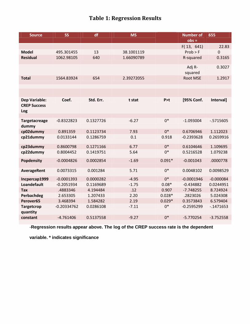
Table 1: Regression Results

Source SS df MS Number of obs =

655

F( 13, 641) 22.83 Model 495.301455 13 38.1001119 Prob > F 0 Residual 1062.98105 640 1.66090789 R-squared 0.3165

Adj R-squared

0.3027

Total 1564.83924 654 2.39272055 Root MSE 1.2917

Dep Variable: CREP Success Log

Coef. Std. Err. t stat P>t [95% Conf. Interval]

Targetacreage dummy

-0.8322823 0.1327726 -6.27 0* -1.093004 -.5715605

cp02dummy 0.891359 0.1123734 7.93 0* 0.6706946 1.112023 cp21dummy 0.0133144 0.1286759 0.1 0.918 -0.2393628 0.2659916

cp23dummy 0.8600798 0.1271166 6.77 0* 0.6104646 1.109695 cp22dummy 0.8004452 0.1419751 5.64 0* 0.5216528 1.079238

Popdensity -0.0004826 0.0002854 -1.69 0.091* -0.001043 .0000778

AverageRent 0.0073315 0.001284 5.71 0* 0.0048102 0.0098529

Incpercap1999 -0.0001393 0.0000282 -4.95 0* -0.0001946 -0.000084 Loandefault -0.2051934 0.1169689 -1.75 0.08* -0.434882 0.0244951 Tax .4883346 4.194484 .12 0.907 -7.748255 8.724924 Perbachdeg 2.653305 1.207433 2.20 0.028* .2823026 5.024308 Perover65 3.468394 1.584282 2.19 0.029* 0.3573843 6.579404 Targetcrop quantity

-0.20334762 0.0286108 -7.11 0* -0.2595299 -.1471653

constant -4.761406 0.5137558 -9.27 0* -5.770254 -3.752558

-Regression results appear above. The log of the CREP success rate is the dependent

variable. * indicates significance

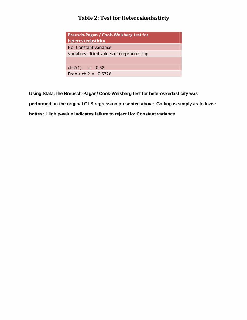
Table 2: Test for Heteroskedasticty

Breusch-Pagan / Cook-Weisberg test for heteroskedasticity

Ho: Constant variance

Variables: fitted values of crepsuccesslog

chi2(1) = 0.32

Prob > chi2 = 0.5726

Using Stata, the Breusch-Pagan/ Cook-Weisberg test for heteroskedasticity was

performed on the original OLS regression presented above. Coding is simply as follows:

hottest. High p-value indicates failure to reject Ho: Constant variance.

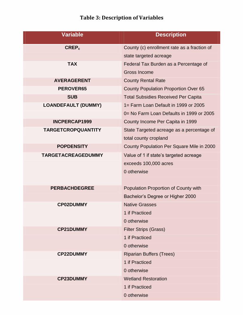
Table 3: Description of Variables

Variable Description

CREPc County (c) enrollment rate as a fraction of

state targeted acreage

TAX Federal Tax Burden as a Percentage of

Gross Income

AVERAGERENT County Rental Rate

PEROVER65 County Population Proportion Over 65

SUB Total Subsidies Received Per Capita

LOANDEFAULT (DUMMY) 1= Farm Loan Default in 1999 or 2005

0= No Farm Loan Defaults in 1999 or 2005

INCPERCAP1999 County Income Per Capita in 1999

TARGETCROPQUANTITY State Targeted acreage as a percentage of

total county cropland

POPDENSITY County Population Per Square Mile in 2000

TARGETACREAGEDUMMY Value of 1 if state’s targeted acreage

exceeds 100,000 acres

0 otherwise

PERBACHDEGREE Population Proportion of County with

Bachelor’s Degree or Higher 2000

CP02DUMMY Native Grasses

1 if Practiced

0 otherwise

CP21DUMMY Filter Strips (Grass)

1 if Practiced

0 otherwise

CP22DUMMY Riparian Buffers (Trees)

1 if Practiced

0 otherwise

CP23DUMMY Wetland Restoration

1 if Practiced

0 otherwise

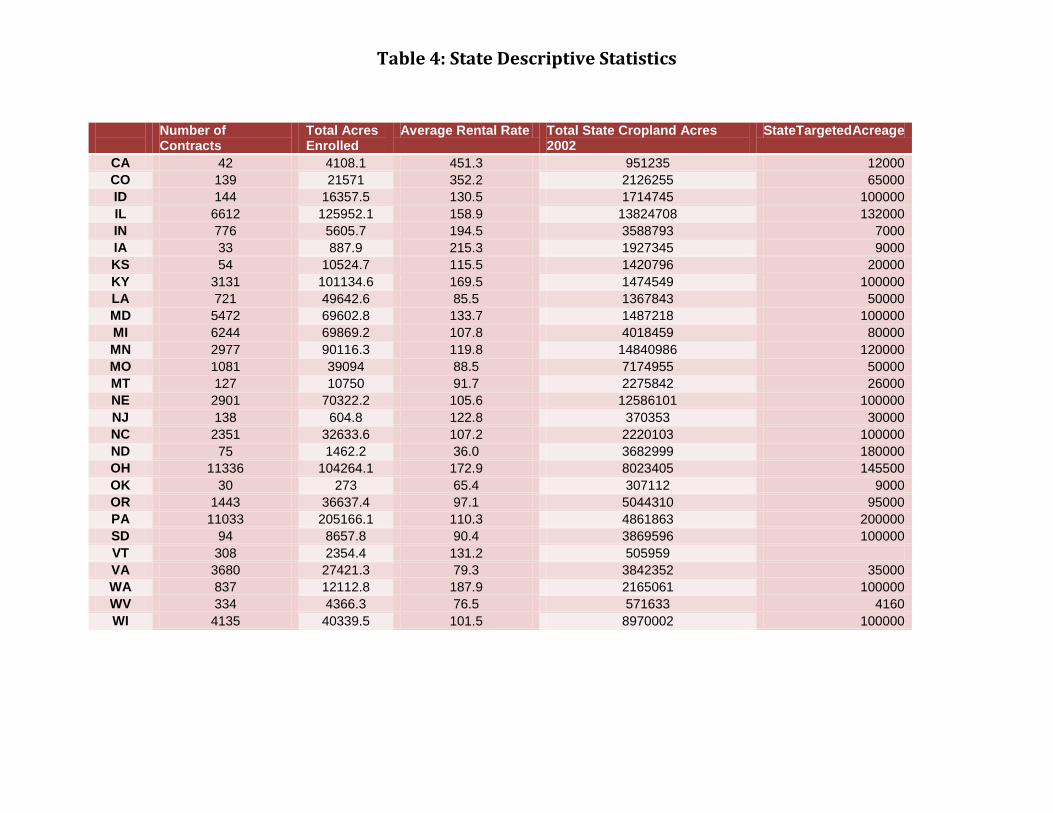
Table 4: State Descriptive Statistics

Number of Contracts

Total Acres Enrolled

Average Rental Rate Total State Cropland Acres 2002

StateTargetedAcreage

CA 42 4108.1 451.3 951235 12000

CO 139 21571 352.2 2126255 65000

ID 144 16357.5 130.5 1714745 100000

IL 6612 125952.1 158.9 13824708 132000

IN 776 5605.7 194.5 3588793 7000

IA 33 887.9 215.3 1927345 9000

KS 54 10524.7 115.5 1420796 20000

KY 3131 101134.6 169.5 1474549 100000

LA 721 49642.6 85.5 1367843 50000

MD 5472 69602.8 133.7 1487218 100000

MI 6244 69869.2 107.8 4018459 80000

MN 2977 90116.3 119.8 14840986 120000

MO 1081 39094 88.5 7174955 50000

MT 127 10750 91.7 2275842 26000

NE 2901 70322.2 105.6 12586101 100000

NJ 138 604.8 122.8 370353 30000

NC 2351 32633.6 107.2 2220103 100000

ND 75 1462.2 36.0 3682999 180000

OH 11336 104264.1 172.9 8023405 145500

OK 30 273 65.4 307112 9000

OR 1443 36637.4 97.1 5044310 95000

PA 11033 205166.1 110.3 4861863 200000

SD 94 8657.8 90.4 3869596 100000

VT 308 2354.4 131.2 505959

VA 3680 27421.3 79.3 3842352 35000

WA 837 12112.8 187.9 2165061 100000

WV 334 4366.3 76.5 571633 4160

WI 4135 40339.5 101.5 8970002 100000

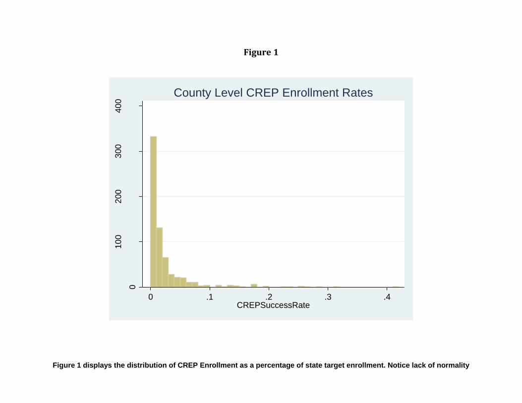
Figure 1

Figure 1 displays the distribution of CREP Enrollment as a percentage of state target enrollment. Notice lack of normality

0

10

020

030

040

0

Fre

quen

cy

0 .1 .2 .3 .4CREPSuccessRate

County Level CREP Enrollment Rates

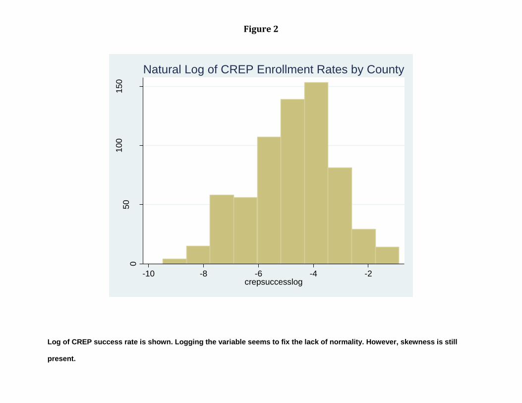
Figure 2

Log of CREP success rate is shown. Logging the variable seems to fix the lack of normality. However, skewness is still

present.

050

10

015

0

Fre

quency (

by C

ounty

)

-10 -8 -6 -4 -2crepsuccesslog

Natural Log of CREP Enrollment Rates by County

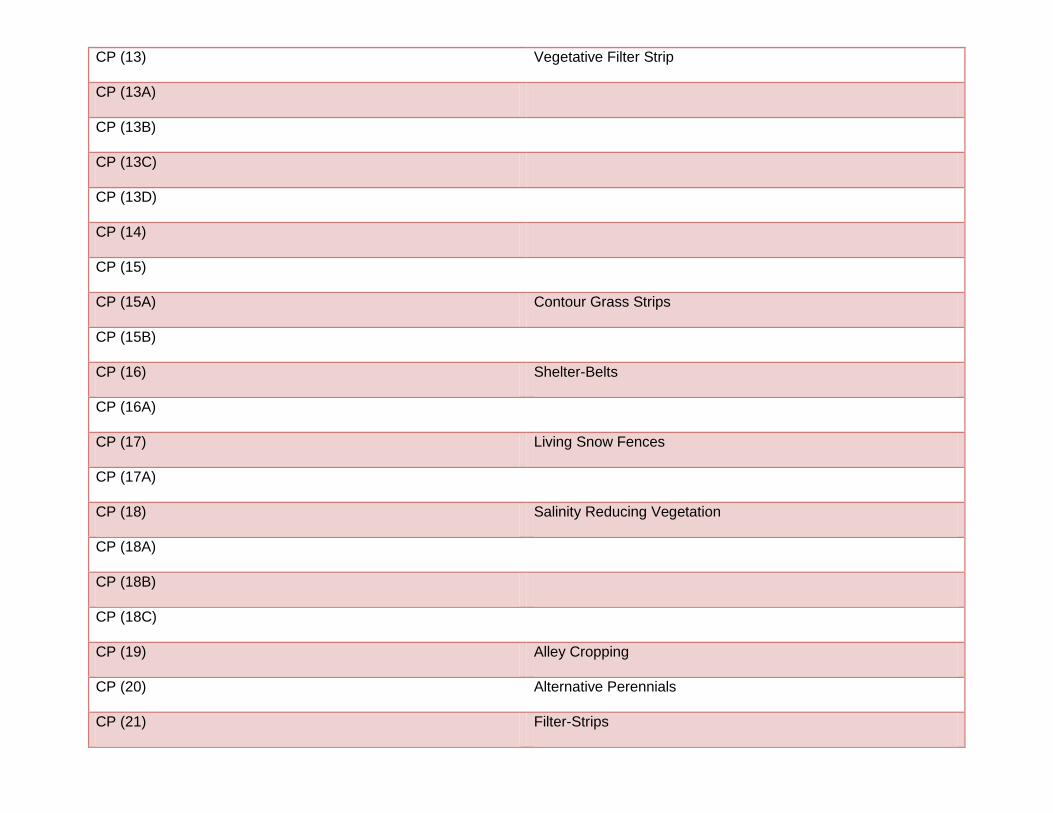
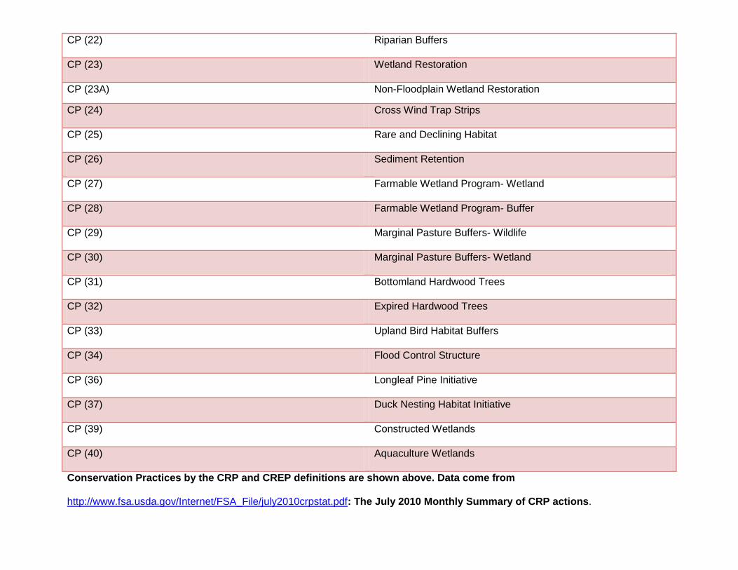
Table 5: Conservation Practice (CP) Definitions

Conservation Practice Description

CP (01) Introduction Grass Planting

CP (02) Native Grass Planting

CP (03) Softwood New Tree Planting

CP (03A) Longleaf Pine/Hardwoods New Tree Planting/

CP (04) Wildlife Habitat

CP (04A)

CP (04B) Wildlife Corridors

CP (05) Field Windbreaks

CP (05A)

CP (06) Diversions

CP (07) Erosion Control Structure

CP (08) Grass Waterways

CP (08A)

CP (09) Shallow Water for Wildlife

CP (10) Existing Grass

CP (11) Existing Trees

CP (12) Wildlife Food Plots

CP (13) Vegetative Filter Strip

CP (13A)

CP (13B)

CP (13C)

CP (13D)

CP (14)

CP (15)

CP (15A) Contour Grass Strips

CP (15B)

CP (16) Shelter-Belts

CP (16A)

CP (17) Living Snow Fences

CP (17A)

CP (18) Salinity Reducing Vegetation

CP (18A)

CP (18B)

CP (18C)

CP (19) Alley Cropping

CP (20) Alternative Perennials

CP (21) Filter-Strips

CP (22) Riparian Buffers

CP (23) Wetland Restoration

CP (23A) Non-Floodplain Wetland Restoration

CP (24) Cross Wind Trap Strips

CP (25) Rare and Declining Habitat

CP (26) Sediment Retention

CP (27) Farmable Wetland Program- Wetland

CP (28) Farmable Wetland Program- Buffer

CP (29) Marginal Pasture Buffers- Wildlife

CP (30) Marginal Pasture Buffers- Wetland

CP (31) Bottomland Hardwood Trees

CP (32) Expired Hardwood Trees

CP (33) Upland Bird Habitat Buffers

CP (34) Flood Control Structure

CP (36) Longleaf Pine Initiative

CP (37) Duck Nesting Habitat Initiative

CP (39) Constructed Wetlands

CP (40) Aquaculture Wetlands

Conservation Practices by the CRP and CREP definitions are shown above. Data come from

http://www.fsa.usda.gov/Internet/FSA_File/july2010crpstat.pdf: The July 2010 Monthly Summary of CRP actions.

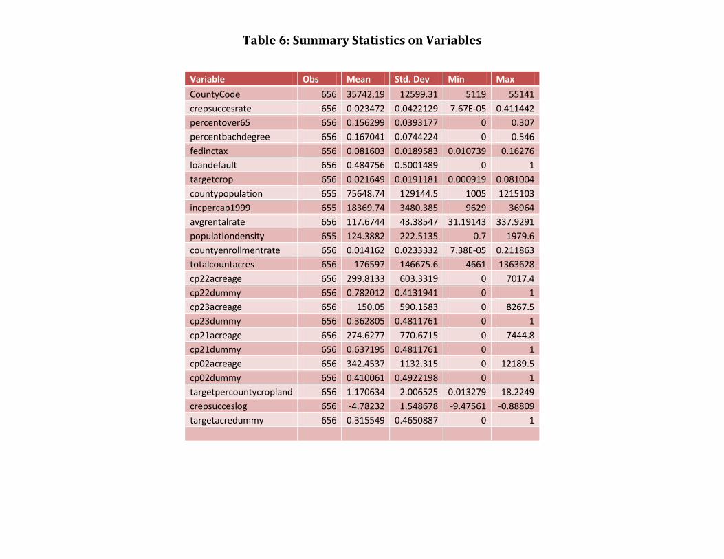
Table 6: Summary Statistics on Variables

Variable Obs Mean Std. Dev Min Max

CountyCode 656 35742.19 12599.31 5119 55141

crepsuccesrate 656 0.023472 0.0422129 7.67E-05 0.411442

percentover65 656 0.156299 0.0393177 0 0.307

percentbachdegree 656 0.167041 0.0744224 0 0.546

fedinctax 656 0.081603 0.0189583 0.010739 0.16276

loandefault 656 0.484756 0.5001489 0 1

targetcrop 656 0.021649 0.0191181 0.000919 0.081004

countypopulation 655 75648.74 129144.5 1005 1215103

incpercap1999 655 18369.74 3480.385 9629 36964

avgrentalrate 656 117.6744 43.38547 31.19143 337.9291

populationdensity 655 124.3882 222.5135 0.7 1979.6

countyenrollmentrate 656 0.014162 0.0233332 7.38E-05 0.211863

totalcountacres 656 176597 146675.6 4661 1363628

cp22acreage 656 299.8133 603.3319 0 7017.4

cp22dummy 656 0.782012 0.4131941 0 1

cp23acreage 656 150.05 590.1583 0 8267.5

cp23dummy 656 0.362805 0.4811761 0 1

cp21acreage 656 274.6277 770.6715 0 7444.8

cp21dummy 656 0.637195 0.4811761 0 1

cp02acreage 656 342.4537 1132.315 0 12189.5

cp02dummy 656 0.410061 0.4922198 0 1

targetpercountycropland 656 1.170634 2.006525 0.013279 18.2249

crepsucceslog 656 -4.78232 1.548678 -9.47561 -0.88809

targetacredummy 656 0.315549 0.4650887 0 1

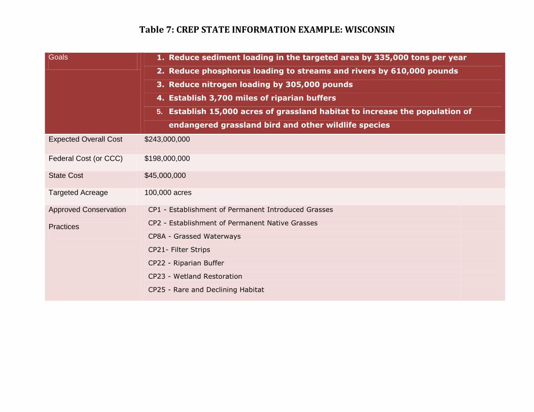
Table 7: CREP STATE INFORMATION EXAMPLE: WISCONSIN

Goals 1. Reduce sediment loading in the targeted area by 335,000 tons per year

2. Reduce phosphorus loading to streams and rivers by 610,000 pounds

3. Reduce nitrogen loading by 305,000 pounds

4. Establish 3,700 miles of riparian buffers

5. Establish 15,000 acres of grassland habitat to increase the population of

endangered grassland bird and other wildlife species

Expected Overall Cost $243,000,000

Federal Cost (or CCC) $198,000,000

State Cost $45,000,000

Targeted Acreage 100,000 acres

Approved Conservation

Practices

CP1 - Establishment of Permanent Introduced Grasses

CP2 - Establishment of Permanent Native Grasses

CP8A - Grassed Waterways

CP21- Filter Strips

CP22 - Riparian Buffer

CP23 - Wetland Restoration

CP25 - Rare and Declining Habitat

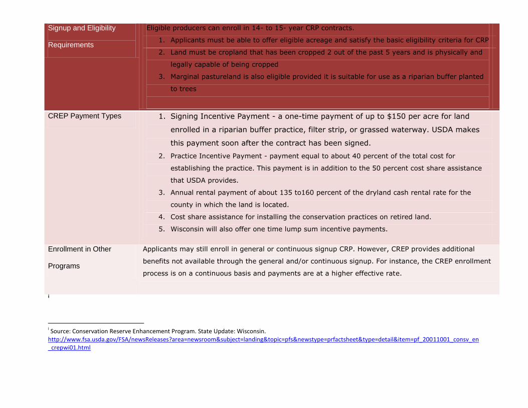
Signup and Eligibility

Requirements

Eligible producers can enroll in 14- to 15- year CRP contracts.

1. Applicants must be able to offer eligible acreage and satisfy the basic eligibility criteria for CRP

2. Land must be cropland that has been cropped 2 out of the past 5 years and is physically and

legally capable of being cropped

3. Marginal pastureland is also eligible provided it is suitable for use as a riparian buffer planted

to trees

CREP Payment Types 1. Signing Incentive Payment - a one-time payment of up to $150 per acre for land

enrolled in a riparian buffer practice, filter strip, or grassed waterway. USDA makes

this payment soon after the contract has been signed.

2. Practice Incentive Payment - payment equal to about 40 percent of the total cost for

establishing the practice. This payment is in addition to the 50 percent cost share assistance

that USDA provides.

3. Annual rental payment of about 135 to160 percent of the dryland cash rental rate for the

county in which the land is located.

4. Cost share assistance for installing the conservation practices on retired land.

5. Wisconsin will also offer one time lump sum incentive payments.

Enrollment in Other

Programs

Applicants may still enroll in general or continuous signup CRP. However, CREP provides additional

benefits not available through the general and/or continuous signup. For instance, the CREP enrollment

process is on a continuous basis and payments are at a higher effective rate.

i

i Source: Conservation Reserve Enhancement Program. State Update: Wisconsin. http://www.fsa.usda.gov/FSA/newsReleases?area=newsroom&subject=landing&topic=pfs&newstype=prfactsheet&type=detail&item=pf_20011001_consv_en_crepwi01.html