The Compositional Effect of Rigorous Teacher

Evaluation on Workforce Quality

Julie Berry Cullen

Cory Koedel

Eric Parsons

October 2016

Improving public sector workforce quality is challenging in sectors such as

education where worker productivity is difficult to assess and manager incentives

are muted by political and bureaucratic constraints. In this paper, we study how

providing information to principals about teacher effectiveness and encouraging

them to use the information in personnel decisions affects the composition of

teacher turnovers. Our setting is the Houston Independent School District, which

recently implemented a rigorous teacher evaluation system. Prior to the new system

teacher effectiveness was negatively correlated with district exit and we show that

the policy significantly strengthened this relationship, primarily by increasing the

relative likelihood of exit for teachers in the bottom quintile of the quality

distribution. Low-performing teachers working in low-achieving schools were

especially likely to leave. However, despite the success, the implied change to the

quality of the workforce overall is too small to have a detectable impact on student

achievement.

Acknowledgements

Cullen is in the department of economics at the University of California, San Diego.

Koedel is in the department of economics and Truman School of Public Affairs, and

Parsons is in the department of economics, at the University of Missouri, Columbia. The

authors gratefully acknowledge financial support from the Laura and John Arnold

Foundation and the National Center for Analysis of Longitudinal Data in Education

Research (CALDER) funded through grant #R305C120008 to American Institutes for

Research from the Institute of Education Sciences, U.S. Department of Education; research

support from the Houston Education Research Consortium, in particular Shauna Dunn,

Holly Heard, Dara Shifrer, and Ruth Turley; and research assistance from Li Tan. The

authors also thank Tom Dee and seminar participants at the Center for Education Policy

Analysis at Stanford University for helpful comments. The views expressed here are those

of the authors and should not be attributed to their institutions, data providers, or the

funders. Any and all errors are attributable to the authors.

1

1. Introduction

Government agencies that provide services, such as education and health, are settings

where it is difficult to observe both inputs and outputs. These are also sectors where there are

ongoing concerns about efficiency and equity. In elementary and secondary education, efforts to

improve the effectiveness of schools have ranged from increases in resources via school finance

reforms, to increased competition via school choice, to performance standards via school

accountability. The success of any of these depends on the quality and commitment of the

workforce.

Recent research provides powerful evidence confirming that high-quality teachers are of

great value to students (Chetty, Friedman, and Rockoff, 2014a/b; Hanushek, 2011; Hanushek and

Rivkin, 2010). A challenge facing school administrators and principals in managing the teacher

workforce is that teacher effectiveness is not easy to measure and is not strongly correlated with

observable characteristics. In this type of setting, improved information about quality can lead to

more productive personnel policies. Given the two-sided nature of matches, better information

may also have equity implications because low-achieving schools struggle to attract and retain

good teachers (Bates, 2015; Clotfelter, Ladd, Vigdor, and Wheeler, 2006).

In this paper, we study the impact of introducing a rigorous teacher evaluation system on

the level and distribution of teacher quality. The context for our study is the Houston

Independent School District (HISD), which is the seventh largest school district in the United

States. The new evaluation system was phased in from 2011 to 2013 and is centered on a

standardized method for annually evaluating teachers. The objective is to generate teacher

performance data that empower principals to exit ineffective and retain effective teachers at

higher rates, as well as improve ongoing skill development. Recognizing that teacher hiring and

2

development also play a role in overall policy efficacy, we focus on how the policy impacted

patterns of attrition by teacher effectiveness.

The empirical analyses rely on administrative data tracking teachers for three years

before to three years after the reform. In order to classify teachers by quality, we construct and

validate proxies for value added to student achievement. Then, using difference-in-differences

and event-study analyses, we show that the relationships between teacher quality and both school

and district exit became more negative in the post-policy period. The key driver is an increase in

the relative likelihood of exit from the district of teachers in the bottom quintile of the quality

distribution, concentrated in low-achieving schools.

As far as impacts on student achievement through the turnover channel, there are two

important issues to consider. First, overall turnover sharply increased after the reform, though it

is unclear what share of this level shift is attributable to the reform. Second, while we document

non-negligible changes to the composition of teacher exits implying an improvement in

workforce quality, differential turnover would have to be much more highly targeted to have a

detectable impact on student achievement. We demonstrate this point in illustrative models that

relate observed school-by-grade-specific exits of teachers to student achievement gains.

Our study contributes in a number of ways to the few existing studies of policies that are

designed to improve workforce quality by providing better information on teacher effectiveness.

In contrast to the rigid rules that characterize the high-profile IMPACT program in Washington

DC, which is studied by Dee and Wyckoff (2015), HISD principals have flexibility in how to act

on the new performance information.1 The presumption is that they know their own schools best

and should be able to leverage their local knowledge. One way to view the HISD system is as a

1 Using a regression discontinuity design, Dee and Wyckoff (2015) find that dismissal threats induce voluntary exit

and raise the performance of low performing teachers who remain.

3

scaled up version of the experimental pilot interventions studied by Sartain and Steinberg

(forthcoming) and Rockoff, Staiger, Kane, and Taylor (2012), with the added feature of a

district-wide emphasis on tying personnel decisions more closely to quality.2 Beyond differences

in the setting in terms of discretion and scale, we also examine the distributional impacts that can

arise when an entire school system is treated.

2. Policy background

HISD has implemented several policies designed to raise staff quality and effort over the

past decade. First, a merit pay program (ASPIRE) was introduced in 2006-07 to reward teachers

and administrators for raising student achievement. Then, four years later, the district began

phased development and implementation of the Effective Teachers Initiative (ETI). This

comprehensive reform effort is designed to improve teacher quality through more effective

recruitment at the front end, individualized professional development in the middle, and targeted

retention and exit on the back end.

The cornerstone of the ETI reform is the implementation of a rigorous teacher evaluation

system intended to provide more informative reviews of teacher performance. The system was

designed by the district during the 2010-11 school year with input from stakeholders and

formally approved by the school board in spring 2011. The new appraisals involve three

components: instructional practice, professional expectations, and student performance. Scores

on the first two components are based on principal observations and reviews conducted inside

and outside the classroom. For instructional practice, a teacher’s skills are evaluated using well-

2 In their New York City experiment, Rockoff et al. (2012) provided principals with improved information on

teacher performance and found that after providing the information, lower-performing teachers were more likely to

exit. Sartain and Steinberg (forthcoming) study a pilot program in Chicago which teachers were more rigorously

evaluated in classroom observations and found that while there was no main effect on teacher exits, the pilot

increased exits for low-rated and non-tenured teachers.

4

defined rubrics that cover setting student expectations, lesson planning, and classroom

management. For the professional expectations component, teachers are evaluated relative to a

set of objective measures of compliance with policies, interactions with colleagues, and

participation in professional development. The student performance scores are based on

estimates of the teacher’s impact on student learning. Teachers are scored on a scale from 1 to 4

on each component, and these are then averaged to deliver a summary rating.

The initial step in transitioning to the new system was ensuring that all teachers were

assigned ratings in 2010-11. Prior to the 2010-11 school year, ratings for almost one in three

teachers were not recorded with the district. Further, ratings were high and did not meaningfully

differentiate teachers (Weisberg et al., 2009). The 2010-11 ratings were based on at least two

classroom observations and, though not formally scored under the new system, these

observations were conducted in an environment where differentiating teachers by quality was a

leading district concern and most principals had already received training. In the following year,

2011-12, teachers were scored under the two new observational components: instructional

practice and professional expectations. Due to delays in approving student performance metrics

for teachers, the student performance measures were not formally incorporated until 2012-13.

Despite this, principals already had access to test-based performance measures for a subset of

teachers, as the SAS Institute has provided proprietary teacher-level value-added estimates

(EVAAS® scores) to HISD for many years as key inputs to the merit pay system. Thus, the shift

in teacher evaluation occurred informally in 2010-11, and at that point principals already had

much of the information that was to be formally incorporated over the next two years.

5

A side effect of the phased implementation is that the official ratings for teachers changed

significantly from 2011-12 to 2012-13.3 When only the observational components were included,

the majority of teachers were labeled effective, with 0.5% ineffective, 10.0% needing

improvement, 57.6% effective, and 31.9% highly effective. Once student performance was

explicitly factored in, these shares changed to 6.0%, 27.7%, 39.7%, and 26.6%, respectively. The

downward shift is due to the fact that the student performance measures are relative, so that some

teachers will necessarily be deemed ineffective, while the other criteria are absolute.

The districtwide emphasis on tying personnel decisions more closely to quality was made

explicit in retention objectives set for district administrators at the onset of the ETI.4 A notable

feature of the new system, which is still in effect today, is that principals are the primary agents

of policy implementation and are given substantial autonomy in translating the information

provided by the assessments into personnel decisions. Further, principals have significant

latitude in exiting teachers since, unlike many districts, teachers at HISD do not have tenure and

most teachers are on one-year contracts.

We examine how the introduction of ETI has affected teacher turnover patterns in ways

that are related to teacher quality. It is important to recognize that the initiative included other

relevant bundled interventions. For example, in the same year as the assessment system was

being developed, the district initiated an early notification program to encourage schools to

identify next-year vacancies earlier in the calendar year (during the prior spring), which may

have allowed for easier teacher transfers between schools. As with other rigorous appraisal

3 Unfortunately we do not have access to personnel evaluations for 2010-11 (or prior years) to document any initial

shifts. 4 Selective retention has continued to be a focus of district policy, as indicated in reports from the superintendent

such as the one submitted for the Board of Education meeting on 12.11.2014, retrieved by the authors online on

06.21.2016 at:

http://www.houstonisd.org/cms/lib2/TX01001591/Centricity/Domain/7949/121114_EVAAS_TeacherRetention_SA

T-ACT.pdf.

6

systems, teachers are provided regular feedback on progress and opportunities for development

to address their specific needs. Over time, new leadership roles were established for effective

teachers to mentor others, and the merit pay system was adjusted to improve alignment with the

new assessment system. Associated changes in the work environment and career opportunities

could alter the relative attractiveness of teaching in the district and of teaching in more and less

advantaged schools. Any impacts on turnover of existing teachers reflect both demand-side and

supply-side responses to the initiative as a whole.

Of course, turnover is also only one channel through which the new human capital

policies could affect the quality of the workforce. Additional objectives were to improve the

quality of incoming teachers and to raise the quality of incumbent teachers. Though our study is

silent on progress on these objectives, turnover is arguably the lever that principals can affect

most, particularly in the short run.

3. Data and summary statistics

We aim to estimate the effects of the new human capital policies on turnover for teachers

of differing effectiveness, across low- and high-achieving schools. We have access to detailed

school, teacher, and student administrative data files for school years 2007-08 through 2013-14.

These data allow us to measure teacher turnover through 2012-13 (where 2013-14 data are used

to measure turnover for 2012-13 teachers), leaving us with a six-year panel centered around

2010-11, which is the first year the human capital policies began to take force.

3.1 Measuring school disadvantage and selecting analysis schools

We begin with a sample of 201 traditional public schools in HISD that were operational

during our sample period and serve students in grades 3 to 8, which are the grade levels for

which we are able to construct measures of teacher quality consistently over the course of our

7

data panel (see below).5 As a summary measure of each school’s context we use the achievement

level, which is defined as the average of students’ math and reading scores on statewide exams,

standardized within grade and year, and taken over the pre-policy years 2007-08 to 2009-10. We

divide schools into three groups based on pre-policy achievement levels: low (bottom quintile),

middle (quintiles 2-4), and high (top quintile).

After classifying schools by achievement, we exclude an additional set of schools due to

a concurrent intervention conducted in HISD as described by Fryer (2014). Fryer (2014) led an

intervention starting in 2010-11—the year that the more rigorous evaluation policies were

initiated—that introduced a bundle of best practices from effective charter schools in 15

traditional elementary and middle schools. The onset of the intervention included changes to

teaching and leadership personnel. To avoid contamination, we drop the schools where Fryer

intervened from our analytic sample. Consistent with his description, all but one of these schools

are in the bottom quintile of achievement. We assign schools to quintiles prior to dropping these

schools so that our school groupings are unconditional. This allows for straightforward

interpretation, with the practical consequence that our sample size of bottom quintile schools is

reduced.6

Table 1 shows summary statistics for the schools included in our analysis, broken down

by achievement group. The top panel shows differences in the characteristics of the student

bodies served across these schools. Beyond the construct-driven differences in achievement,

low-achieving schools serve a disproportionate share of black students and students with English

5 We exclude the few schools from which less than five teacher-year observations are available for these grades,

where a teacher-year observation requires an EVAAS® score. These cases are most likely due to errors in the school

code assigned to the teacher. 6 In the appendix (Appendix Table A.4) we show that our main findings are qualitatively similar if we include these

schools in the analytic sample.

8

as a second language, while high-achieving schools serve markedly fewer economically

disadvantaged students.

3.2 Measuring teacher turnover and selecting analysis teachers

In addition to measuring school exits, we decompose school exits into exits from the

district and transfers to other schools within the district. A complication we face is that the

staffing data provided to us in 2013-14 include only teachers. In all previous years the staffing

data include all positions. For consistency, throughout our analysis we identify a teacher as

having exited the school at the conclusion of year t if the teacher is not observed teaching in the

school in year t+1. Thus, we code switches to non-teaching positions (e.g., school leadership) as

exits. In the appendix, we confirm that our results are substantively the same if we exclude the

last year of data and code position changes as non-exits.7

We define teacher turnover by looking forward in the data one year. A benefit of using a

single-year measure instead of a multi-year measure is that we can calculate turnover for more

years. That said, the limitation of the single-year exit measures is that they are noisy and

overstate exit rates. It has been well documented that teachers – particularly young teachers –

move in and out of the workforce (Grissom and Reininger, 2012). We therefore test robustness to

using alternative two-year definitions for campus and district exit, where a teacher is classified as

having exited if she is also not present in year t+2.

The middle panel of Table 1 shows single-year turnover rates for math teachers in grades

3-8 in the pre-policy period. Pre-policy turnover is 13.7% at low- and middle-achieving schools,

versus 12.1% at high-achieving schools. The difference is driven primarily by a lower rate of

7 More specifically, while the overall exit rates that we estimate annually decline slightly if we re-code position

changes as non-exits (on the order of 1-2 percentage points), the cross-year and pre-post comparative results are

qualitatively unaffected. See Appendix Table A.1.

9

within-district transfer from high-achieving schools. Unsurprisingly, two-year exit rates (not

shown) indicate marginally lower turnover by approximately 0.4 percentage points, or 3

percent.8

3.3 Measuring teacher quality

Critical to our analysis is being able to measure teacher effectiveness in a comparable

way over the full sample period. While teacher experience and education levels might be

candidates, the literature has consistently shown that these observable characteristics explain

little of the variation in student learning and are not consistently linked to teacher quality

(Aaronson, Barrow, and Sander, 2007; Hanushek and Rivkin, 2006; Harris and Sass, 2011). We

also have scores from principal appraisals for the components that were part of the official

evaluation system in 2011-12 and 2012-13, but not only are these unavailable in prior years, the

observational components are difficult to compare across campuses with differentially

challenging environments and map much more weakly to student learning (Kane et al., 2013;

Steinberg and Garrett, 2016; Whitehurst, Chingos, and Lindquist, 2014).

For these reasons, we construct quality measures derived from the value-added estimates

that have been provided to principals for teachers in tested grades and subjects for many years at

HISD. These teacher-specific EVAAS® scores are single-year measures of student test score

growth produced using a propriety method developed by the SAS Institute. Although the

technical estimation details differ from standard value-added models, conceptually they are

similar (Ballou, Sanders, and Wright, 2004). Teachers’ EVAAS® scores are estimated from

regressions of student achievement on a set of indicators for each teacher the student had in the

current and prior two years, as well as indicators for subject, grade, and year. These scores are

8 The pre-policy turnover statistics in Table 1 are similar to turnover statistics provided for grade 4 to 5 teachers in

New York City by Ronfeldt, Loeb, and Wyckoff (2013).

10

available to us back to the 2006-07 school year, and we restrict our analysis to teachers in grades

3-8 who have been assigned math or reading EVAAS® scores.

Because the single-year estimates are quite noisy,9 we construct a more informative

measure of teacher effectiveness by combining multiple years of teachers’ scores per the

following regression based on Chetty, Friedman, and Rockoff (2014a):

0ikt iktV ikt- 1V δ

(1)

In equation (1),

Vikt is teacher i’s EVAAS® score in subject k and year t, ikt-V is a vector of

teacher i’s EVAAS® scores in the same subject in years prior to year t, and

ikt is an

idiosyncratic error term. The EVAAS® scores are normalized by subject and year. The fitted

values from the regression, 0ˆ ˆˆ

iktV ikt- 1V δ , are jackknifed quality measures where a value of

one, for example, implies that the teacher is one standard deviation above average in the true

distribution for teachers in the district.10 Because not all teachers have a complete panel of prior

scores to be used in the estimation of equation (1), separate regression models are estimated for

all possible combinations as in Chetty, Friedman, and Rockoff (2014a). We do require, though,

that the teacher have a time t EVAAS® score to be included in the sample, which ensures the

individual is teaching the relevant subject contemporaneously. An implication of including only

scores from years prior to t as explanatory variables is that first-year teachers are necessarily

excluded from the sample. However, our reliance on prior-year performance guards against

9 Brehm, Imberman, and Lovenheim (2015) show that relative rankings of teachers under the merit pay system

based on EVAAS® estimates vary greatly from year to year. 10 The jackknifed quality measures are not renormalized to have a standard deviation of one, and in fact have a

standard deviation less than one. Theoretically, a one-unit change in the jackknifed measures corresponds to a one

standard deviation change in the distribution of teacher quality (see, e.g., Chetty, Friedman, Rockoff, 2014b).

11

survivor bias, since otherwise teachers who persist would be more likely to have quality

measures available.11

It is important to demonstrate that our measures meaningfully capture teacher

effectiveness in raising student achievement. Recent studies show that conceptually similar

jackknifed measures based on value-added are forecast-unbiased estimates of teacher quality in

other contexts (see Bacher-Hicks, Kane, and Staiger, 2014; Chetty, Friedman, and Rockoff,

2014a). Adopting their methods, we test whether our measures have the same property by

examining whether changes in teacher quality at the school-by-grade level caused by staffing

changes accurately predict changes in student test scores, as would be expected if the measures

are unbiased. For example, if a teacher with high measured effectiveness moves to a new school

and/or a different grade, test scores for students in the new school-by-grade combination should

increase in the year after the change. Moreover, if the quality metric is properly scaled, the

magnitude of the change in teacher quality should predict the magnitude of the change in student

achievement.

We implement the forecasting test by estimating the following regression model,

weighted by time t school-by-grade enrollment:

0 1ˆ

sgkt sgkt t iktA V sgt 2ΔX γ (2)

The dependent variable, sgktA , is the change in the average test score on the statewide exam

(standardized by grade and year) between years t and t-1 for school s and grade g in subject k.

Only students taught by a teacher with an available effectiveness measure at time t are included

11 Note that our jackknifed measures rely on more observations for years that are later in the panel, so it may seem

that a relative reduction in noise could confound our estimated relationships over time. Not only have we

empirically confirmed that our results are robust to restricting the backward-looking windows to be comparable

across years, but the implicit shrinkage is also a theoretical argument against this concern (Jacob and Lefgren,

2008).

12

in the regression and used to calculate

A sgkt. In addition to year effects, the control set includes

ˆsgktV , which is the change in average measured teacher quality, and sgtΔX , which captures the

change in student demographics between years t and t-1.

For the purposes of the validation exercise, we make adjustments to the way teacher

quality is measured, which is why the variable is denoted with a prime in equation (2). First, we

rescale teachers’ EVAAS® scores to student exam score units. This permits one-to-one

forecasting between the teacher quality metrics and the dependent variable. Then, we calculate

leave-two-year-out jackknife estimates, where neither the time t nor the t-1 teacher scores are

included in ikt-V . This is important to remove the influence of the mechanical correlation

between the change in average student test scores between those two periods and the estimation

error in the annual teacher scores. We conduct the test for both purely backward looking quality

measures and, to increase precision, for measures that also allow post-period performance data to

inform the current-year quality measure (as in Chetty, Friedman, and Rockoff 2014a).12

We test the null hypothesis

1 1 separately for math and reading and report the results

in Table 2. With the caveat that our tests are less powerful than in previous studies that exploit

larger datasets, our findings are consistent with the jackknifed quality measures being forecast

unbiased predictors of future student achievement. Specifically, we cannot reject that the

coefficient on the change in teacher quality is unity in any of the models. Yet, the larger standard

errors in the reading regressions leave open the possibility of non-negligible bias and suggest

more individual-level prediction errors. For these reasons our reading-based teacher quality

estimates are less informative, which is consistent with findings in previous research (Backes et

12 Jackknifing based on pre- and post-period data is not a problem for this exercise because the internally valid

estimates of forecasting bias can still be obtained even if survivors are over-sampled.

13

al., 2016; Lefgren and Sims, 2012). Thus, we choose to present results restricted to teachers for

whom we can observe effectiveness in teaching math in the main text, and present selected

results for reading in the appendix. The reading results are very similar to the math results (see

Appendix Tables A.2 and A.3).

The bottom panel of Table 1 shows how math teacher quality is distributed across schools

in the pre-policy period. In addition to our measure of effectiveness, where the numbers reported

are in standard deviations of the teacher distribution, we also include other observable teacher

characteristics. Based on our measure, Table 1 shows that teacher quality is not evenly

distributed across the district. More low-quality teachers and fewer high-quality teachers are

found at low-achieving schools. Low-achieving schools also employ teachers with less

experience, but teachers at these schools tend to be more educated. A simple regression of our

jackknifed quality measure in math on teacher experience and indicators for education levels

using the pre-policy data yields an R-squared of just 0.01.

Finally, it is important to note that our quality measures are not directly available to

school principals. Instead, principals have access to year-by-year EVAAS® scores and

observational assessments, in addition to other indicators of quality that we do not observe. In

2012-13, the first year that all components of the assessment were formally scored, our measure

of quality explains approximately 24 percent of the variation in overall appraisal ratings among

our sample of teachers with EVAAS® scores. It explains 13, 4, and 23 percent of the

instructional practice, professionalism, and student learning components, respectively, where the

student learning component is a categorical rating based on the contemporaneous EVAAS®

score and at least one other student-learning measure that is determined in collaboration between

the teacher and principal. One reason that the correlation with the classroom-observation

14

component is not higher is that scores on these types of best practices metrics have been shown

to be sensitive to the composition of students in the classroom (Steinberg and Garrett, 2016;

Whitehurst, Chingos, and Lindquist, 2014). By building our program evaluation around our

validated but unobserved jackknife measures, we can determine whether teacher and principal

responses to the new system are affecting workforce quality in a way that is likely to have direct

implications for student achievement.

4. Empirical strategy

To estimate effects on turnover, we estimate difference-in-differences models of the

following form, specified as linear probability models:

0 1 2 3ist t it t it s istY Post Q Post Q stX β (3)

In equation (3),

Yist is a binary variable indicating whether teacher i at school s exits the school

(or exits the district or transfers to another school) at the conclusion of year t. tPost is an

indicator set to one for 2010-11 and later years.

Qit is our measure of teacher quality. In some

variants of the model we include

Qit as a continuous variable, and in others we divide teachers

into quality quintiles and include a vector of indicator variables for the quintile assignments.

Shrinkage is implicit in the jackknifing procedure and thus our estimates will not be affected by

attenuation bias from using a generated regressor as would be the case with a standard linear

predictor (Jacob and Lefgren, 2008). The X-vector contains teacher characteristics that might

have independent effects on turnover, such as race, gender, experience, and education. Our

findings are not sensitive to which subset of these characteristics we include in the regressions,

nor are they sensitive to omitting the X-vector entirely. Finally,

s is a school fixed effect to

allow for fixed school attributes that affect teacher attrition rates, and

ist is an error term.

Throughout we report standard errors clustered at the school level.

15

The objective of the model is to identify shifts in the relationship between teacher quality

and exit. We also report estimates of

1 to give a sense of how the overall teacher exit rate is

changing over time. To the extent that these changes can be attributed to policy implementation,

they are indications of the policy impact on the extensive margin. Of course, it is difficult to rule

out that other time-varying factors are at play when estimating these simple differences. Thus,

we emphasize estimates of

3, which is the coefficient on the interaction between the post-

reform indicator and teacher quality. This parameter provides an indication of the policy impact

on the intensive margin – that is, on a per-exit basis it provides a measure of how workforce

quality is changing due to push and pull factors associated with the reform. Since a primary goal

was to increase exit of ineffective teachers and increase retention of effective teachers, we would

expect to find a negative coefficient on the interaction.

A necessary condition for identifying the policy impact on relative exit rates is that pre-

policy trends in exit rates between teachers of different levels of quality are the same. To explore

the validity of the design, as well as to provide evidence on the time pattern of any responses, we

also estimate event time models. For these time-disaggregated models, we include a full set of

year effects and year effects interacted with teacher quality.

In addition to estimating average impacts, we also study heterogeneity across schools to

shed light on distributional effects. For these models, we add interactions between the time and

quality variables with indicators for schools that are low (bottom-quintile) and high (top-quintile)

achieving based on pre-period achievement. Principals at low-achieving schools might have

benefited more from the information provided by the new system, but might also have less

capacity to respond. Demand for effective teachers likely increased system-wide, opening up the

16

possibility for the best teachers to trade-up in terms of school environment and making retention

tougher at the bottom (Bates, 2015).

5. Effects of the reform on turnover

5.1 Descriptive analysis

We begin by visually documenting trends in exit and turnover rates in Figure 1. The

figure shows district-wide trends for our three different mobility measures: school exit, district

exit, and school transfer. The former is the sum of the two latter measures. School years in the

figure, and in all figures and tables to follow, are identified by the spring year – e.g., the 2010-11

school year is labeled as 2011. The figure shows that turnover by all three measures began to rise

at the conclusion of the 2010-11 school year. Of total school exits, roughly half of the observed

increase is attributable to an increase in district exits, and half is due to an increase in within-

district school transfers.

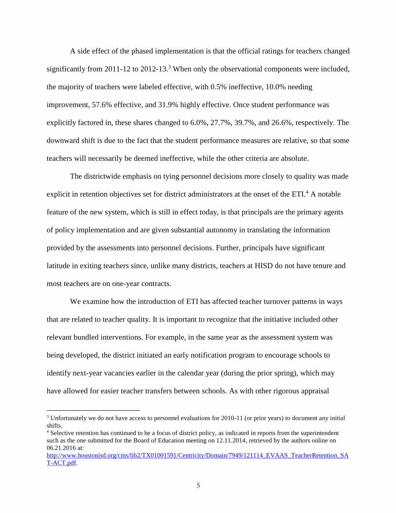
Figure 2 provides similar information but divides teachers into groups based on our

measure of quality. Teachers are assigned to the following groups based on their placement in

the quality distribution each year: bottom quintile (least effective), middle quintiles (quintiles 2-

3-4), and top quintile (most effective). Panels A, B, and C report differences in the rates of

school exit, district exit, and school transfers across teacher quality groups. It is visually apparent

that the school exit rate increased more quickly in the post-policy period for the least effective

teachers relative to other teachers, driven primarily by district exits. Although instances of school

transfers are higher in the post-policy years overall (Figure 1), no systematic change in the

relationship between teacher quality and school switching is apparent in Figure 2.

5.2 Estimation results

We estimate the models described in Section 4 to assess the significance and robustness

17

of the patterns illustrated in Figures 1 and 2. First, Table 3 shows results from equation (3) where

we enter the teacher-quality measure into the regressions linearly. We report results for the full

specification, which is our preferred model, but in unreported results our estimates are very

similar if we use sparser variants of the model that exclude teacher characteristics and even

school fixed effects. For each turnover outcome, we present models that aggregate the pre- and

post-policy time periods and models that fully disaggregate years. All control variables except

for the post-period indicator (or year indicators) are mean-centered in the regressions, including

the school indicator variables, so that the intercept can be interpreted as the exit rate at the mean

values of all covariates.13

The general patterns from Figures 1 and 2 are reflected in the model estimates and

confirmed to be statistically significant in Table 3. For example, in the model of district exits,

our estimate in column (2a) implies that a teacher who is one standard deviation above average

in the quality distribution is an additional 6.3 percentage points less likely to exit the district

during the post-policy relative to the pre-policy period. The estimated impact is attenuated for

the inclusive school exit outcome in column (1a) since, as suggested by Figure 2 and shown in

column (3a), there is no change in the relationship between school switching and teacher quality.

The event time models in the table are useful for two reasons. First, they document that

there were no pre-trends in turnover by quality (i.e., the coefficients on the interactions between

teacher quality and the 2009 and 2010 indicators, which are estimated relative to the holdout year

2008, are small and statistically insignificant). Moreover, though the causal impact on overall

turnover rates is not well identified by our model, the pre-period trend is in the opposite direction

13 The mean-centering does not affect model fit or the coefficients on the key parameters interacting time with

teacher quality. It is used only to improve interpretability of the results with regard to the overall exit rate (Dalal and

Zickar, 2012).

18

of what we see in the post period. A second benefit of the disaggregated models is that, in

principle, they allow us to test how impacts evolve over time. We do tend to find the largest and

most statistically significant impacts in the final year, but are unfortunately not well enough

powered to differentiate these from the estimates for the other reform years.

Next, in Table 4 we show results from models where we replace the linear quality

measures in equation (3) with indicators for teachers’ quality-quintile groups. The indicator

identifying teachers in the middle quintiles (2-3-4) is omitted for comparison. We do not show

the intercept coefficients and interactions to preserve space. Consistent with what we show in

Figure 2, Table 4 confirms that the post-policy period is marked by a large and statistically

significant increase in the likelihood of school and district exit for low-performing teachers

relative to middle and high performing teachers. Between these two latter groups, there is no

divergence in exit rates.

Table 5 reports on the robustness of our findings to two adjustments to the analysis. First,

in the left panel, we consider the sensitivity of our results to using a 2-year exit measure for

school and district exits. That is, rather than coding exits based on looking forward just one year

in the data, we look forward two years to determine whether the exiting teacher remained either

(a) out of the school or (b) out of the district. When we make this definitional change, we are no

longer able to examine outcomes for the 2013 teacher cohort. Thus, we report results from

models covering the 2008-2012 cohorts using the one-year and two-year exit definitions, which

are otherwise comparable to the results we show in Table 3. Although the overall exit levels are

slightly lower with the two-year definition, the patterns in our estimates are very similar using

either measure.

19

In the right panel of Table 5 we return to using our full dataset and single-year exit

measures and replicate the analysis in Table 3 (columns 1a, 2a, and 3a) after restricting the

models to include only schools that did not experience a principal change. Changes in leadership

are one mechanism by which the new evaluation system could influence the workforce.

Approximately 38 percent of schools in our analytic sample retained the same principal over the

course of the full data panel (this number is in line with data on principal tenure in Texas as

reported by Branch, Hanushek, and Rivkin, 2012). The results are generally similar to what we

report in Table 3, which suggests that principal changes are not a critical mediator of our

findings.

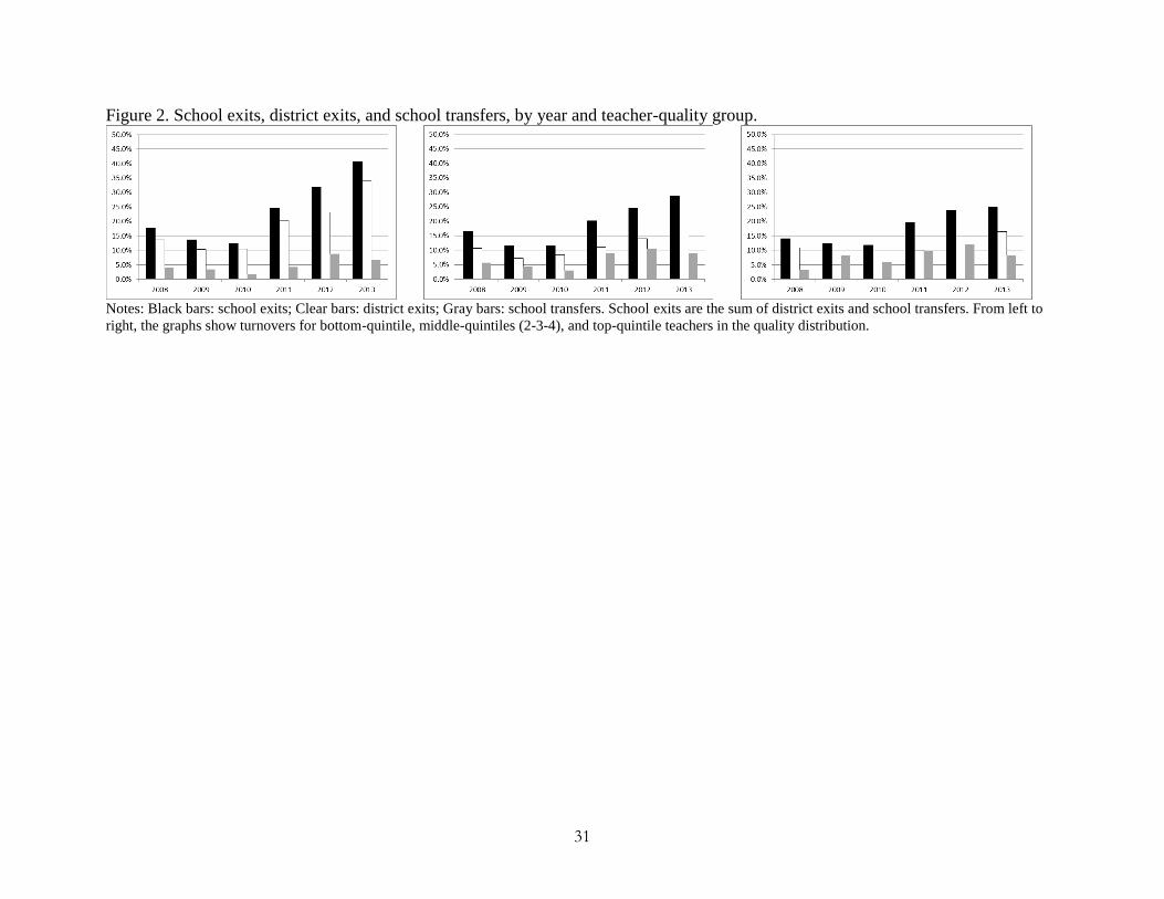
Table 6 shows results from models run separately for teachers by experience level. We

divide teachers into three groups based on experience: ≤ 5 years, 6-20 years, and more than 20

years, and run the model for each turnover outcome separately for each group. Overall exit rates

increased for all experience groups and although noisily estimated, the pre-post change in the

relationship between quality and exit/transfer is similar across experience groups. The

consistency by experience is surely facilitated in part by the absence of tenure at HISD and the

fact that teachers are primarily on 1-year contracts. This result would be unlikely to generalize to

districts with strong tenure protections (Sartain and Steinberg, forthcoming).

Finally, in Table 7 we estimate models that are otherwise the same as those shown in

Table 3, but we replace our jackknifed teacher quality measures with single-year EVAAS®

scores. For ease of interpretation, we do not alter the analytic sample in Table 7 (although in

principle using single-year EVAAS® scores would allow us to include novice teachers and,

more generally, teachers new to teaching mathematics in grades 3-8). The results clearly show

that turnover in the post period aligns much more strongly with our jackknifed quality measures

20

– which are unobserved by principals and district officials, at least directly – than with the

noisier current-year EVAAS® scores, which are observed. This result is consistent with the

interpretation that personnel decisions under the reform are being made based on a totality of

evidence that is superior to the single-year, noisy quality information embodied by the annual

EVAAS® measures, as intended in a combined-measure evaluation system.

6. Heterogeneity in effects across schools

6.1 Descriptive analysis

In Figure 3, we replicate the information shown in Figure 1, but separately for each

school type. Recall that we divide schools into three groups based on their pre-policy location in

the distribution of average achievement in math and reading: bottom quintile (low-achieving),

middle quintiles (quintiles 2-3-4), and top quintile (high-achieving). The figure shows that while

exit rates increased across all three groups in the post-period (which is consistent with Figure 1),

there has been a disproportionate increase at the lowest-achieving schools.

Figure 4 further divides teachers by quality within the same school groups. Reading

across a row in Figure 4 holds the school-achievement group fixed, and reading down a column

holds the teacher quality group fixed. Although the graphs in the figure cut the data thinly, and

therefore noise is an issue, they suggest several interesting patterns. For instance, the first row of

graphs shows school-exit, district-exit, and school-transfer patterns at low-achieving schools, by

teacher type. The clear bars across the first row illustrate that low-performing teachers at low-

achieving schools were much more likely to exit the district in the post-policy period relative to

the pre-policy period. However, when looking at rates of school exit (black bars), the relative

difference shrinks because school-transfer rates (gray bars) climb for middle- and high-

performing teachers at low-achieving schools. Bates (2015) suggests a potential mechanism –

21

namely, more effective teachers under the new system have more prominent signals of their

ability than had previously been the case, and can leverage these signals into more desirable

teaching positions. In the absence of true compensating wage differentials, as is typical in the

public education context, teachers will prefer positions that are more desirable along non-

pecuniary dimensions (Greenberg and McCall, 1974).14

Turning to middle-achieving schools, although the difference in district exit rates

between low- and high-performing teachers is smaller than for low-achieving schools, it is

similarly signed and there is not an offsetting school-changer effect. For high-achieving schools,

there is no clear visual change in the relationship between exit and teacher quality between the

pre- and post-policy periods. If anything, the differences look stronger for middle- and high-

performing teachers owing to the lower pre-period exit rates of these teachers from high-

achieving schools.

6.2 Estimation results

As discussed in Section 4, we add interaction terms to equation (3) to test whether the

patterns suggested by Figures 3 and 4 are statistically significant in our difference-in-differences

specification. Table 8 presents results from models that use the linear quality measures, like in

Table 3, but with the added interactions for school type. The heterogeneity parameters of interest

interact the post-policy indicator with teacher quality and school type, where bottom- and top-

quintile schools are included in the model and compared to the holdout group of middle-quintile

schools. The bottom two rows of Table 8 show coefficient estimates and standard errors for these

triple interactions.

14 Teachers may prefer to work in higher-achieving schools for a variety of reasons. Survey evidence suggests that

while teachers do prefer to work with higher-SES students, perhaps because this requires less effort, simple non-

pecuniary benefits that are correlated with student SES, like better administrative support and shorter commute

times, are more important in pushing teachers toward high-SES schools (Horng, 2009).

22

To interpret the findings in Table 8, first note that the post-policy effect on the

relationship between each measure of turnover and teacher quality for middle-achieving schools

is shown in row 4. By virtue of their omission from the model as the holdout group, the double

interaction of quality and the post-period indicator is the effect for these schools. For school and

district exits, the estimates in Table 8 for middle-quintile schools are similar to, albeit slightly

larger than, the analogous global estimates shown in Table 3. They imply a workforce improving

change in the composition of exiters. Also as in Table 3, there is no systematic impact on the

relationship between school transfers and teacher quality for middle-quintile schools.

For bottom quintile schools, the triple interaction coefficients in the second-to-last row of

Table 8 indicate the quality effect at these schools relative to middle quintile schools. Although

the estimates are noisy and merely suggestive, they imply that some of the positive effect on

workforce quality for bottom-quintile schools is dulled by a positive relationship between teacher

quality and school transfers among teachers at these schools. For top-quintile schools, the triple-

interaction estimates indicate that the net effect of the policies is essentially null. More

specifically, the triple-interaction terms in the final row of Table 8 more than offset the baseline

effects in row 4.

In results that we do not report for brevity, we also estimate similar models that

additionally divide teachers into quintile groups and use these groups in place of the linear

quality measures, so that these models have interactions across school and teacher groupings

akin to what we show visually in Figure 4. Although the coefficients are signed in directions

consistent with what would be expected based on results from the linear quality models in Table

8, we lack statistical power to draw further inference from the binned interactions.

23

7. Discussion and interpretation

Given that we measure teacher quality in terms of effectiveness and validate the

predictive power of our measures, it is reasonable to expect that gains in student learning would

align with the change in the quality composition of exiters. However, whether or not gains are

realized also depends on any impacts on the quality of teacher entrants and on effort among

teachers who remain (Rothstein, 2015). Inference is further clouded by the high turnover rates at

HISD post-ETI. Since turnover increases as much as it does, to the extent that this turnover is

attributed to the policy and adversely affects achievement, it could imply net losses for students.

In order to gauge how the turnover aspects of the policy might be expected to affect

student achievement, we estimate models of changes in school-by-grade achievement of the

following form:

0 2 3 4 5 6sgt sgt sgt sgt sgt sgt s t sgtA TO BQ MQ TQ UK u sgt 1ΔX β (4)

In equation (4), sgtA is the difference in average test scores across student cohorts in school s

and grade g from period t-1 to t.15 The focal explanatory variables are (a) the change in the level

of teacher turnover the two cohorts were exposed to, sgtTO , and (b) the share of teachers exiting

between years by quality groups denoted by sgtBQ , sgtMQ , sgtTQ , and sgtUK for bottom-quintile,

middle-quintiles, top-quintile, and unknown teacher quality, respectively. We include the

unknown category to account for teachers without jackknifed quality measures, which makes

these four categories exhaustive. The turnover variables are scaled by teachers’ instructional

percentages in the given subject prior to exit. For example, if a teacher provides one-fourth of the

mathematics instruction for a school-by-grade cell, exits the school between years t-1 and t, and

15 Each observation is weighted by time t school-by-grade student enrollment, and standard errors are clustered at

the school-by-grade level.

24

is a bottom quintile teacher, then sgtBQ is coded as 0.25 (assuming no other bottom quintile

teachers in the school-by-grade cell exit at the same time). The vector sgtΔX captures changes in

student demographic characteristics across cohorts corresponding to the test-score comparison,

while s and t are school and year fixed effects, respectively. This model is similar to the

model estimated by Adnot et al. (2016) except we control not only for the level of teacher

turnover across cohorts, which captures changes in the composition of teachers, but also for

changes in exposure to turnover, which captures differential disruption.

The results of estimating this model are shown in Table 9. While the results should be

viewed cautiously because they rely on realized differences in turnover across grades, they seem

quite plausible. The estimated coefficient on the change in turnover implies that there is a

disruption effect (Hanushek, Rivkin and Schiman, 2016; Ronfeldt, Loeb, and Wyckoff, 2013),

which we estimate to be 0.088 student-level standard deviations for a school-by-grade cell that

experiences 100 percent turnover. The estimated coefficients on the exit shares of bottom,

middle, and high quality teachers of 0.172, 0.066, and -0.169, respectively, align closely with the

average jackknifed effectiveness measures for each group, which are -0.132, 0.012, and 0.175,

respectively (converted to student standard deviation units).

Taking the estimates in Table 9 at face value, we can combine them with results from our

earlier analysis to conduct a back-of-the-envelope calculation of the overall achievement effect

of the compositional change in exits. Figure 5 re-packages our results from above in a way that is

better suited to illustrate the total achievement effect. The figure shows model-based estimates of

the compositional shifts in quality for school and district exiters due to the new evaluation

system, taking the district exit rate in the pre- and post-policy periods as given. The figure

highlights a clear shift toward more low-performing teacher exits, although there are still many

25

middle- and high-performing teachers who exit. Combining the information in Figure 5 with our

estimates of the impact of exits by teachers of different qualities from Table 9, the expected

average change in achievement per turnover increases very little from the pre- to post-policy

period – just 0.007 and 0.005 student standard deviations for school and district exiters,

respectively.16 Moreover, these compositional estimates do not account for the negative general

disruption effect of turnovers.

While our analysis up to this point consistently points toward a compositional change in

turnovers that is directionally in line with improved student achievement, we conclude that exits

are not targeted well enough to induce meaningful achievement gains.

8. Conclusion

We study the effects on workforce composition of the introduction of a new, more-

rigorous teacher evaluation system in the Houston Independent School District. The new system

has clearly affected the composition of exiting teachers, primarily by increasing the exit rate

among low performers relative to higher-performing teachers. Policy activity along this

dimension has been concentrated at low-achieving schools within the district; at high-achieving

schools, there is little indication that the nature of personnel decisions changed in the post-policy

years.

Our analysis illustrates the potential for more rigorous teacher evaluations to improve

student outcomes via better-informed personnel decisions, but also highlights a critical challenge

associated with improving workforce quality via selective attrition. In short, in the system we

16 The figure is constructed using estimates from Table 4 for the relative changes in teacher exit by quality group.

The compositional change estimates are mechanically dependent on the total district exit rate in the pre- and post-

policy periods, where it is unclear how much of the shift is causally attributable to the policy. However, qualitatively

our estimates of the per-turnover effect on achievement are unaffected by reasonable adjustments to the baseline

rate. For example, if we impose that the total exit rate increased by half of the observed rate from the pre- to post-

policy period in our calculations, the achievement effect sizes increase but remain small, at around 0.010 student

standard deviations.

26

study there are simply too many poorly targeted exits in the post-policy period (by middle- and

top-performing teachers) for the net policy effect on achievement to be meaningful.

Stepping back from our narrow policy context, a possible complementary intervention in

such a situation would be to offer more competitive wages that better reflect the large differences

in teacher quality documented here and elsewhere to stem the tide of higher-quality teacher exits,

as argued in Rothstein (2015). Although HISD has attempted to better align pay with

productivity via the aforementioned APSIRE program, that program has faced challenges and

our results are consistent with the difficulty the district has faced in better aligning compensation

to productivity (Brehm, Imberman, and Lovenheim, 2015; Shifrer, Turley, and Heard, 2013).

There are also other ways that the new system is designed to improve instruction and student

outcomes about which our study is silent – notably via recruitment and greater improvement

among incumbent teachers – but on the dimension of selective attrition, the compositional effects

have not been large enough to measurably improve student achievement.

27

References

Aaronson, Daniel, Lisa Barrow and William Sander. 2007. Teachers and Student Achievement in

the Chicago Public High Schools. Journal of Labor Economics 25(1), 95-135.

Adnot, Melinda, Thomas Dee, Veronica Katz and James Wyckoff. 2016. Teacher Turnover,

Teacher Quality, and Student Achievement in DCPS. NBER Working Paper No. 21922.

Bacher-Hicks, Andrew, Thomas J. Kane and Douglas O. Staiger. 2014. Validating Teacher

Effect Estimates Using Changes in Teacher Assignments in Los Angeles. NBER Working Paper

No. 20657.

Backes, Ben, James Cowan, Dan Goldhaber, Cory Koedel, Luke Miller and Zeyu Xu. 2016. The

Common Core Conundrum: To What Extent Should We Worry that Changes to Assessments and

Standards Will Affect Test-Based Measures of Teacher Performance. CALDER Working Paper

No. 152.

Ballou, Dale, William Sanders and Paul Wright. 2004. Controlling for Student Background in

Value-Added Assessment of Teachers. Journal of Educational and Behavioral Statistics 29(1),

37-65.

Bates, Michael. 2015. Public and Private Learning in the Market for Teachers: Evidence from

the Adoption of Value-Added Measures. Unpublished manuscript.

Branch, Gregory F., Eric A. Hanushek and Steven G. Rivkin. 2012. Estimating the Effect of

Leaders on Public Sector Productivity: The Case of School Principals. NBER Working Paper

No. 17803.

Brehm, Margaret, Scott A. Imberman and Michael F. Lovenhiem. 2015. Achievement Effects of

Individual Performance Incentives in a Teacher Merit Pay Tournament. NBER Working Paper

No. 21598.

Chetty, Raj, John N. Friedman and Jonah E. Rockoff. 2014a. Measuring the Impacts of Teachers

I: Evaluating Bias in Teacher Value-Added Estimates. American Economic Review 104(9),

2593-2632.

Chetty, Raj, John N. Friedman and Jonah E. Rockoff. 2014b. Measuring the Impacts of Teachers

II: Teacher Value-Added and Student Outcomes in Adulthood. American Economic Review

104(9), 2633-79.

Clotfelter, Charles T., Helen F. Ladd, Jacob L. Vigdor and Justin Wheeler. 2006. High-poverty

Schools and the Distribution of Teachers and Principals. North Carolina Law Review 85: 1345-

1379.

28

Dalal, Dev K., and Michael J. Zickar. 2012. Some Common Myths about Centering Predictor

Variables in Moderated Multiple Regression and Polynomial Regression. Organizational

Research and Methods 15(3), 339-362.

Dee, Thomas and James Wyckoff. 2015. Incentives, Selection, and Teacher Performance:

Evidence from IMPACT. Journal of Policy Analysis and Management 34(2), 267-297.

Fryer, Roland G. 2014. Injecting Charter School Best Practices into Traditional Public Schools:

Evidence from Field Experiments. Quarterly Journal of Economics 129(3), 1355-1407.

Greenberg, David, and John McCall. 1974. Teacher Mobility and Allocation. Journal of Human

Resources 9(4), 480-502.

Grissom, Jason A. and Michelle Reininger. 2012. Who Comes Back? A Longitudinal Analysis of

the Re-Entry Behavior of Exiting Teachers. Education Finance and Policy 7(4): 425-454.

Hanushek, Eric A. 2011. The Economic Value of Higher Teacher Quality. Economics of

Education Review 30(3), 266-479.

Hanushek, Eric A., and Steven G. Rivkin. 2006. "Teacher Quality." In Handbook of the

Economics of Education Vol. 1, ed. Eric A. Hanushek and Finis Welch, 1051-78. Amsterdam:

North-Holland.

Hanushek, Eric A. and Steven G. Rivkin. 2010. Generalizations about Using Value-Added

Measures of Teacher Quality. American Economic Review 100(2), 267-271.

Hanushek, Eric A., Steven G. Rivkin and Jeffrey C. Schiman. 2016. Dynamic Effects of Teacher

Turnover on the Quality of Instruction. NBER Working Paper No. 22472.

Harris, Douglas N. and Tim R. Sass. 2011. Teacher Training, Teacher Quality and Student

Achievement. Journal of Public Economics 95(7-8), 798-812.

Horng, Eileen Lai. 2009. Teacher Tradeoffs: Disentangling Teachers’ Preferences for Working

Conditions and Student Demographics. American Educational Research Journal 46(3), 690-717.

Jacob, Brian and Lars Lefgren. 2008. Can Principals Identify Effective Teachers? Evidence on

Subjective Performance Evaluation in Education. Journal of Labor Economics 26(1), 101-136.

Kane, Thomas J., Daniel F. McCaffrey, Trey Miller and Douglas O. Staiger. 2013. Have We

Identified Effective Teachers? Validating Measures of Effective Teaching Using Random

Assignment. Seattle, WA: Bill and Melinda Gates Foundation.

Lefgren, Lars and David P. Sims. 2012. Using Subject Test Scores Efficiently to Predict Teacher

Value-Added. Educational Evaluation and Policy Analysis 34(1), 109-121.

29

Rockoff, Jonah E., Douglas O. Staiger, Thomas J. Kane and Eric S. Taylor. 2012. Information

and Employee Evaluation: Evidence from a Randomized Intervention in Public Schools.

American Economic Review 102(7), 3184-3213.

Ronfeldt, Matthew, Susanna Loeb and James Wyckoff. 2013. How Teacher Turnover Harms

Student Achievement. American Educational Research Journal 50(1), 4-36.

Rothstein, Jesse. 2015. Teacher Quality Policy When Supply Matters. American Economic

Review 105(1), 100-130.

Sartain, Lauren and Matthew P. Steinberg (forthcoming). Teachers’ Labor Market Responses to

Performance Evaluation Reform: Experimental Evidence from Chicago Public Schools. Journal

of Human Resources.

Shifrer, Dara, Ruth Lopez Turley and Holly Heard. 2013. Houston Independent School District’s

ASPIRE Program: Estimated Effects of Receiving Financial Awards. Policy Report. Houston

Educational Research Consortium.

Steinberg, Matthew P. and Rachel Garret. 2016. Classroom Composition and Measured Teacher

Performance: What do Teacher Observation Scores Really Measure? Educational Evaluation

and Policy Analysis 38(2), 293-317.

Weisberg, Daniel, Susan Sexton, Jennifer Mulhern and David Keeling. 2009. The Widget Effect:

Our National Failure to Acknowledge and Act on Differences in Teacher Effectiveness. New

York: The New Teacher Project.

Whitehurst, Grover J., Matthew M. Chingos, and Katharine M. Lindquist. 2014. Evaluating

Teachers with Classroom Observations: Lessons Learned in Four Districts. Washington, DC:

Brown Center on Education Policy at Brookings.

30

Figure 1. School exits, district exits, and school transfers, by year.

Notes: Black bars: school exits; Clear bars: district exits; Gray bars: school transfers.

School exits are the sum of district exits and school transfers.

31

Figure 2. School exits, district exits, and school transfers, by year and teacher-quality group.

Notes: Black bars: school exits; Clear bars: district exits; Gray bars: school transfers. School exits are the sum of district exits and school transfers. From left to

right, the graphs show turnovers for bottom-quintile, middle-quintiles (2-3-4), and top-quintile teachers in the quality distribution.

32

Figure 3. School exits, district exits, and school transfers, by year and pre-policy achievement group of school.

Notes: Black bars: school exits; Clear bars: district exits; Gray bars: school transfers. School exits are the sum of district exits and school transfers. From left to

right, the graphs show turnovers at bottom-quintile, middle-quintiles (2-3-4), and top-quintile schools in the pre-policy (average of reading and math)

achievement distribution.

33

Figure 4. School exits, district exits, and school transfers, by year, pre-policy achievement group of school, and teacher-quality group.

Notes: Black bars: school exits; Clear bars: district exits; Gray bars: school transfers. School exits are the sum of district exits and school transfers. Row 1:

bottom-quintile schools; Row 2: middle-quintiles schools; Row 3: top-quintile schools; Column 1: bottom-quintile teachers; Column 2: middle-quintiles teachers;

Column 3: top-quintile teachers.

34

Figure 5. School and district exits, by teacher-quality group in the pre- and post-policy periods.

School exits:

Pre-policy

Post-policy

District exits:

Pre-policy

Post-policy

Notes: Black: bottom-quintile teachers; Clear: middle-quintiles teachers (quintiles 2-3-4); Gray: top-quintile

teachers. The figures are derived from model-based estimates of the proportions of exiting teachers by quality-

quintile group in the pre- and post-policy periods, for school and district exiters, taking the pre- and post-policy total

exit rates as given.

35

Table 1. Summary statistics for pre-policy years 2007-08 through 2009-10.

Schools by achievement level

Low Middle High

Student characteristics

Average achievement z-scores -0.295 -0.061 0.484

Percent free lunch 55.3% 57.6% 33.4%

Percent reduced price lunch 8.8% 11.0% 11.0%

Percent black 40.8% 20.7% 20.1%

Percent Hispanic 56.9% 75.3% 47.2%

Percent ESL 16.7% 8.1% 4.8%

Number of grade 3-8 students tested 25,125 86,628 44,560

Math teacher turnover

Exited the school in t+1 13.7% 13.7% 12.1%

Exited the district in t+1 8.5% 9.0% 8.8%

Transferred to another school in t+1 5.2% 4.7% 3.3%

Math teacher characteristics

Jackknifed quality measure -0.012 0.047 0.098

Percent bottom quintile 21.5% 21.4% 14.5%

Percent top quintile 14.1% 21.2% 21.0%

Years of experience 9.9 10.7 12.0

Percent with 1 to 5 years experience 34.6% 33.5% 30.6%

Percent with master’s degree 34.6% 30.5% 28.5%

Percent with doctoral degree 2.5% 1.4% 1.3%

Number of teacher-years 483 2508 970 Notes: The columns present summary statistics for analysis schools divided into three groups based on pre-policy

achievement levels, averaged across reading and math: bottom quintile, middle three quintiles, and top quintile. The

bottom-quintile sample is smaller because treated schools in Fryer’s 2014 study are omitted and also because low-

achieving schools have lower enrollment on average. School exits are the sum of district exits and school transfers.

As described in the text, our analytic dataset excludes first-year teachers and correspondingly these teachers are also

excluded from the teacher summary statistics.

36

Table 2. Test for bias in jackknifed teacher quality measures.

1̂

P-value

(H0: γ1=1)

Number of school-

grade-year cells

(1) (2) (3)

Backward looking

Grades 4-8, math 0.833

(0.106)

0.12 2612

Grades 4-8, reading 0.946

(0.163)

0.74 2630

Backward and forward looking

Grades 4-8, math 0.999

(0.077)

0.99 3413

Grades 4-8, reading 0.974

(0.131)

0.85 3423

Notes: Coefficients and standard errors as estimated by equation (2) in the main text are reported in column (1).

Column (2) reports p-values from tests of the null hypothesis of forecast-unbiasedness, and column (3) reports the

number of school-by-grade-by-year cells used in the regressions. The backward-looking measures include only

teacher scores from year t-2 and earlier. The backward and forward-looking measures also include scores from year

t+1 and later.

37

Table 3. Impacts of the new evaluation system on turnover, by linear math teacher quality. Dependent variable is an indicator for:

School exit District exit School transfer

(1a) (1b) (2a) (2b) (3a) (3b)

Intercept 0.125

(0.006)**

0.148

(0.011)**

0.085

(0.004)**

0.105

(0.009)**

0.040

(0.004)**

0.043

(0.007)**

Intercept*POST 0.137

(0.012)**

0.083

(0.008)**

0.054

(0.008)**

Intercept*2009 -0.031

(0.015)**

-0.035

(0.012)**

0.003

(0.011)

Intercept*2010 -0.035

(0.015)**

-0.026

(0.012)**

-0.009

(0.009)

Intercept*2011 0.062

(0.019)**

0.025

(0.014)*

0.037

(0.013)**

Intercept*2012 0.119

(0.018)**

0.050

(0.013)**

0.069

(0.013)**

Intercept*2013 0.172

(0.019)**

0.123

(0.017)**

0.049

(0.012)**

Teacher quality -0.008

(0.015)

-0.025

(0.032)

-0.034

(0.012)**

-0.029

(0.027)

0.026

(0.009)**

0.004

(0.017)

Teacher quality*POST -0.061

(0.021)**

-0.063

(0.019)**

0.002

(0.016)

Teacher quality*2009 0.024

(0.036)

-0.009

(0.030)

0.033

(0.024)

Teacher quality*2010 0.024

(0.037)

-0.002

(0.031)

0.027

(0.023)

Teacher quality*2011 -0.001

(0.039)

-0.042

(0.034)

0.040

(0.028)

Teacher quality*2012 -0.020

(0.044)

-0.047

(0.038)

0.027

(0.032)

Teacher quality*2013 -0.074

(0.043)*

-0.090

(0.038)**

0.016

(0.022)

Teacher characteristics X X X X X X

School fixed effects X X X X X X

R-squared 0.101 0.108 0.081 0.089 0.078 0.080

N (Teacher-year) 7800 7800 7800 7800 7800 7800

Notes: ** Denotes statistical significance at the 5 percent level; * Denotes statistical significance at the 10 percent

level. Standard errors clustered by school are reported in parentheses. Observations for teachers during the 2011,

2012, and 2013 school years are coded as “POST” in columns 1a, 2a, and 3a. In these columns, the parameters for

the variables interacted with POST are estimated relative to the pre-period years. In columns 1b, 2b, and 3b, the

year-specific parameters are estimated relative to 2008, which is the first year of our data panel. All variables in the

regressions other than the post indicator (or year indicators) are mean-centered so the intercept can be interpreted as

the exit rate at the mean values of all covariates. The coefficients for all variables other than the teacher quality

measures and the intercept, both interacted with time, are excluded for brevity.

38

Table 4. Impacts of the new evaluation system on turnover, by math teacher quality quintile. Dependent variable is an indicator for:

School exit District exit School transfer

(1a) (1b) (2a) (2b) (3a) (3b)

Bottom quintile 0.012

(0.015)

0.012

0.030

0.027

(0.013)**

0.033

(0.024)

-0.015

(0.008)*

-0.021

(0.017)

Top quintile 0.006

(0.015)

-0.012

(0.025)

-0.009

(0.011)

0.010

(0.023)

0.015

(0.010)

-0.023

(0.015)

Bottom quintile*POST 0.076

(0.023)**

0.089

(0.022)**

-0.013

(0.013)

Top quintile*POST -0.007

(0.023)

0.003

(0.020)

-0.010

(0.016)

Bottom quintile*2009 0.000

(0.038)

-0.010

(0.032)

0.010

(0.022)

Bottom quintile*2010 0.000

(0.037)

-0.007

(0.032)

0.007

(0.020)

Bottom quintile*2011 0.050

(0.038)

0.068

(0.034)**

-0.018

(0.022)

Bottom quintile*2012 0.074

(0.045)

0.070

(0.039)*

0.004

(0.028)

Bottom quintile*2013 0.109

(0.051)**

0.114

(0.047)**

-0.005

(0.025)

Top quintile*2009 0.032

(0.036)

-0.030

(0.027)

0.062

(0.026)**

Top quintile*2010 0.023

(0.033)

-0.026

(0.028)

0.049

(0.022)**

Top quintile*2011 0.023

(0.036)

-0.006

(0.032)

0.029

(0.025)

Top quintile*2012 0.028

(0.036)

-0.010

(0.033)

0.038

(0.027)

Top quintile*2013 -0.014

(0.045)

-0.032

(0.041)

0.018

(0.027)

Teacher characteristics X X X X X X

School fixed effects X X X X X X

R-squared 0.102 0.110 0.083 0.092 0.078 0.081

N (Teacher-year) 7800 7800 7800 7800 7800 7800

Notes: The specifications are the same as in Table 3, other than that indicators for the top and bottom quintiles

replace the continuous quality variable. The omitted group includes teachers in quality quintiles 2, 3, and 4. See

notes to Table 3.

39

Table 5. Tests for robustness of impacts of the new evaluation system on turnover, by linear math teacher quality.

1-year exit definition

2008-2012 cohorts

2-year exit definition

2008-2012 cohorts

No principal change

1-year exit definition

2008-2013 cohorts

School exit District exit School exit District exit School exit District exit School transfer

(1a) (2a) (1b) (2b) (3) (4) (5)

Intercept 0.128

(0.005)**

0.086

(0.003)**

0.124

(0.005)**

0.079

(0.003)**

0.104

(0.006)**

0.077

(0.005)**

0.027

(0.005)**

Intercept*POST 0.113

(0.013)**

0.058

(0.009)**

0.112

(0.013)**

0.051

(0.008)**

0.102

(0.013)**

0.064

(0.010)**

0.038

(0.010)**

Teacher quality -0.008

(0.015)

-0.031

(0.012)**

-0.011

(0.015)

-0.031

(0.012)**

-0.004

(0.021)

-0.033

(0.018)*

0.029

(0.011)**

Teacher quality* POST -0.037

(0.024)

-0.046

(0.020)**

-0.034

(0.024)

-0.041

(0.019)**

-0.069

(0.028)**

-0.048

(0.023)**

-0.021

(0.021)

Teacher characteristics X X X X X X X

School fixed effects X X X X X X X

R-squared 0.097 0.078 0.098 0.077 0.085 0.073 0.067

N (Teacher-year) 6656 6656 6656 6656 3054 3054 3054 Notes: The estimates in this table are comparable to estimates in Table 3 and the notes to Table 3 apply. In the left panel, we examine teacher cohorts in 2008-12

only, for whom we can define exits looking forward both 1 and 2 years in the data, to examine the sensitivity of our findings to the exit definition holding all else

equal. In the right panel, we return to using our primary single-year exit definition and 2008-13 cohorts, but restrict the sample to include only schools in which

there was not a principal change over the course of the data panel.

40

Table 6. Impacts of the new evaluation system on turnover by teacher experience and linear math teacher quality. School exit District exit School transfer

Exp ≤ 5 5< Exp≤20 Exp>20 Exp≤ 5 5<Exp≤20 Exp>20 Exp≤ 5 5< Exp≤20 Exp>20

(1a) (1b) (1c) (2a) (2b) (2c) (3a) (3b) (3c)

Intercept 0.187

(0.009)**

0.102

(0.007)**

0.084

(0.013)**

0.133

(0.008)**

0.062

(0.005)**

0.074

(0.012)**

0.054

(0.007)**

0.040

(0.005)**

0.010

(0.006)*

Intercept*POST 0.136

(0.021)**

0.132

(0.013)**

0.158

(0.027)**

0.081

(0.017)**

0.072

(0.010)**

0.115

(0.025)**

0.054

(0.015)**

0.060

(0.010)**

0.043

(0.012)**

Teacher quality -0.008

(0.030)

-0.012

(0.020)

0.045

(0.034)

-0.039

(0.025)

-0.043

(0.014)**

0.042

(0.034)

0.031

(0.019)*

0.031

(0.014)**

0.004

(0.017)

Teacher quality*POST -0.077

(0.050)

-0.054

(0.029)*

-0.101

(0.056)*

-0.065

(0.042)

-0.054

(0.023)**

-0.109

(0.055)**

-0.012

(0.032)

0.000

(0.023)

0.008

(0.023)

Teacher characteristics X X X X X X X X X

School fixed effects X X X X X X X X X

R-squared 0.153 0.118 0.246 0.138 0.093 0.208 0.116 0.110 0.279

N (Teacher-year) 2409 4174 1217 2409 4174 1217 2409 4174 1217

Notes: The estimates in this table are comparable to estimates in Table 3 and the notes to Table 3 apply. Each column reports results from a separate regression

estimated for teachers by experience group, where teachers are divided into three groups: ≤ 5 years, 6-20 years, and more than 20 years experience.

41

Table 7. Impacts of the new evaluation system on turnover, by linear math teacher quality and

using current-year EVAAS® scores in place of jackknifed measures.

School exit District exit School transfer

(1) (2) (3)

Intercept 0.125

(0.006)**

0.085

(0.004)**

0.040

(0.004)**

Intercept*POST 0.136

(0.011)**

0.082

(0.008)**

0.054

(0.008)**

Current-year EVAAS -0.015

(0.006)**

-0.015

(0.005)**

0.000

(0.004)

Current-year EVAAS*POST -0.021

(0.010)**

-0.023

(0.008)**

0.002

(0.006)

Teacher characteristics X X X

School fixed effects X X X

R-squared 0.103 0.079 0.077

N (Teacher-year) 7800 7800 7800 Notes: The estimates in this table are comparable to estimates in Table 3 and the notes to Table 3 apply. The

specification is the same as in Table 3 but replaces the jackknifed quality measure with the current-year EVAAS®

score.

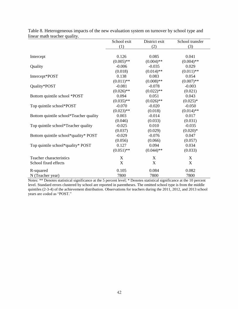
42

Table 8. Heterogeneous impacts of the new evaluation system on turnover by school type and

linear math teacher quality. School exit District exit School transfer

(1) (2) (3)

Intercept 0.126

(0.005)**

0.085

(0.004)**

0.041

(0.004)**

Quality -0.006

(0.018)

-0.035

(0.014)**

0.029

(0.011)**

Intercept*POST 0.138

(0.011)**

0.083

(0.008)**

0.054

(0.007)**

Quality*POST -0.081

(0.026)**

-0.078

(0.022)**

-0.003

(0.021)

Bottom quintile school *POST 0.094

(0.035)**

0.051

(0.026)**

0.043

(0.025)*

Top quintile school*POST -0.070

(0.023)**

-0.020

(0.018)

-0.050

(0.014)**

Bottom quintile school*Teacher quality 0.003

(0.046)

-0.014

(0.033)

0.017

(0.031)

Top quintile school*Teacher quality -0.025

(0.037)

0.010

(0.029)

-0.035

(0.020)*

Bottom quintile school*quality* POST -0.029

(0.056)

-0.076

(0.066)

0.047

(0.057)

Top quintile school*quality* POST 0.127

(0.051)**

0.094

(0.044)**

0.034

(0.033)

Teacher characteristics X X X

School fixed effects X X X

R-squared 0.105 0.084 0.082

N (Teacher year) 7800 7800 7800 Notes: ** Denotes statistical significance at the 5 percent level; * Denotes statistical significance at the 10 percent

level. Standard errors clustered by school are reported in parentheses. The omitted school type is from the middle

quintiles (2-3-4) of the achievement distribution. Observations for teachers during the 2011, 2012, and 2013 school

years are coded as “POST.”

43

Table 9. Estimated effects of turnover on student achievement.

Notes: ** Denotes statistical significance at the 5 percent level; * Denotes statistical significance at the 10 percent

level. Standard errors clustered by school are reported in parentheses. The turnover shares are scaled by teachers’

instructional percentages in the given subject prior to exit. The quality groupings, inclusive of the unknown quality

group (i.e., teachers without jackknifed quality measures), are exhaustive.

Dependent variable: Difference in average test scores

across cohorts within a school-grade

ΔTurnover -0.088

(0.025)**

Share bottom-quintile exit 0.172

(0.055)**

Share middle-quintiles exit 0.066

(0.035)*

Share top-quintile exit -0.169

(0.061)**

Share unknown-quality exit 0.137

(0.056)**

School-grade characteristics X

School fixed effects X

R-squared 0.093

N (School-grade-year) 2824

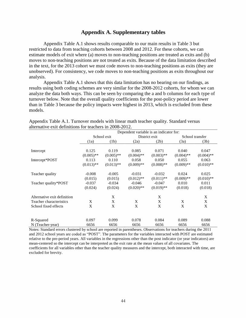
44

Appendix A. Supplementary tables

Appendix Table A.1 shows results comparable to our main results in Table 3 but

restricted to data from teaching cohorts between 2008 and 2012. For these cohorts, we can

estimate models of exit where (a) moves to non-teaching positions are treated as exits and (b)

moves to non-teaching positions are not treated as exits. Because of the data limitation described

in the text, for the 2013 cohort we must code moves to non-teaching positions as exits (they are

unobserved). For consistency, we code moves to non-teaching positions as exits throughout our

analysis.

Appendix Table A.1 shows that this data limitation has no bearing on our findings, as

results using both coding schemes are very similar for the 2008-2012 cohorts, for whom we can

analyze the data both ways. This can be seen by comparing the a and b columns for each type of

turnover below. Note that the overall quality coefficients for the post-policy period are lower

than in Table 3 because the policy impacts were highest in 2013, which is excluded from these

models.

Appendix Table A.1. Turnover models with linear math teacher quality. Standard versus

alternative exit definitions for teachers in 2008-2012. Dependent variable is an indicator for:

School exit District exit School transfer

(1a) (1b) (2a) (2b) (3a) (3b)

Intercept 0.125

(0.005)**

0.119

(0.005)**

0.085

(0.004)**

0.071

(0.003)**

0.040

(0.004)**

0.047

(0.004)**

Intercept*POST 0.113

(0.013)**

0.110

(0.013)**

0.058

(0.009)**

0.050

(0.008)**

0.055

(0.009)**

0.063

(0.010)**

Teacher quality -0.008

(0.015)

-0.005

(0.015)

-0.031

(0.012)**

-0.032

(0.011)**

0.024

(0.009)**

0.025

(0.010)**

Teacher quality*POST -0.037

(0.024)

-0.034

(0.024)

-0.046

(0.020)**

-0.047

(0.019)**

0.010

(0.018)

0.011

(0.018)

Alternative exit definition X X X

Teacher characteristics X X X X X X

School fixed effects X X X X X X

R-Squared 0.097 0.099 0.078 0.084 0.089 0.088

N (Teacher-year) 6656 6656 6656 6656 6656 6656

Notes: Standard errors clustered by school are reported in parentheses. Observations for teachers during the 2011

and 2012 school years are coded as “POST”. The parameters for the variables interacted with POST are estimated

relative to the pre-period years. All variables in the regressions other than the post indicator (or year indicators) are

mean-centered so the intercept can be interpreted as the exit rate at the mean values of all covariates. The

coefficients for all variables other than the teacher quality measures and the intercept, both interacted with time, are

excluded for brevity.

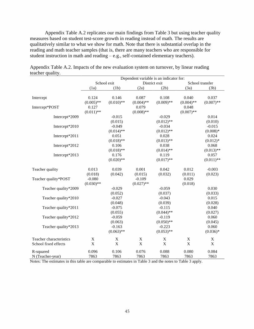
45

Appendix Table A.2 replicates our main findings from Table 3 but using teacher quality

measures based on student test-score growth in reading instead of math. The results are

qualitatively similar to what we show for math. Note that there is substantial overlap in the

reading and math teacher samples (that is, there are many teachers who are responsible for

student instruction in math and reading – e.g., self-contained elementary teachers).

Appendix Table A.2. Impacts of the new evaluation system on turnover, by linear reading

teacher quality. Dependent variable is an indicator for:

School exit District exit School transfer

(1a) (1b) (2a) (2b) (3a) (3b)

Intercept 0.124

(0.005)**

0.146

(0.010)**

0.087

(0.004)**

0.108

(0.009)**

0.040

(0.004)**

0.037

(0.007)**

Intercept*POST 0.127

(0.011)**

0.079

(0.008)**

0.048

(0.007)**

Intercept*2009 -0.015

(0.015)

-0.029

(0.012)**

0.014

(0.010)

Intercept*2010 -0.049

(0.014)**

-0.034

(0.012)**

-0.015

(0.008)*

Intercept*2011 0.051

(0.018)**

0.028

(0.013)**

0.024

(0.012)*

Intercept*2012 0.106

(0.018)**

0.038

(0.014)**

0.068

(0.013)**

Intercept*2013 0.176

(0.020)**

0.119

(0.017)**

0.057

(0.011)**

Teacher quality 0.013

(0.018)

0.039

(0.042)

0.001

(0.015)

0.042

(0.032)

0.012

(0.011)

-0.003

(0.023)

Teacher quality*POST -0.080

(0.030)**

-0.109

(0.027)**

0.029

(0.018)

Teacher quality*2009 -0.029

(0.052)

-0.059

(0.037)

0.030

(0.033)

Teacher quality*2010 -0.027

(0.048)

-0.043

(0.039)

0.015

(0.028)

Teacher quality*2011 -0.075

(0.055)

-0.115

(0.044)**

0.040

(0.027)

Teacher quality*2012 -0.059

(0.063)

-0.119

(0.050)**

0.060

(0.045)

Teacher quality*2013 -0.163

(0.063)**

-0.223

(0.053)**

0.060

(0.036)*

Teacher characteristics X X X X X X

School fixed effects X X X X X X

R-squared 0.096 0.106 0.076 0.088 0.080 0.084

N (Teacher-year) 7863 7863 7863 7863 7863 7863

Notes: The estimates in this table are comparable to estimates in Table 3 and the notes to Table 3 apply.

46

Appendix Table A.3 replicates our main findings from Table 4 but using teacher quality

measures based on student test-score growth in reading instead of math. The results are

qualitatively similar to what we show for math, although in the reading models there is some

evidence that top-quintile teacher exit rates declined in the post-policy period. Note that there is

substantial overlap in the reading and math teacher samples (that is, there are many teachers who

are responsible for student instruction in math and reading – e.g., self-contained elementary

teachers).

Appendix Table A.3. Impacts of the new evaluation system on turnover, by reading teacher

quality quintile. School exit District exit School transfer

(1a) (1b) (2a) (2b) (3a) (3b)

Bottom quintile -0.021

(0.015)

-0.043

(0.025)*

-0.018

(0.014)

-0.039

(0.021)*

-0.003

(0.008)

-0.004

(0.015)

Top quintile 0.014

(0.015)

-0.002

(0.031)

-0.005

(0.011)

-0.003

(0.024)

0.020

(0.008)**

0.001

(0.014)

Bottom quintile*POST 0.054

(0.026)**

0.073

(0.024)**

-0.019

(0.015)

Top quintile*POST -0.039

(0.024)

-0.046

(0.019)**

0.008

(0.015)

Bottom quintile*2009 0.043

(0.037)

0.042

(0.030)

0.001

(0.022)

Bottom quintile*2010 0.023

(0.030)

0.021

(0.027)

0.002

(0.015)

Bottom quintile*2011 0.060

(0.040)

0.075

(0.037)**

-0.015

(0.021)

Bottom quintile*2012 0.072

(0.040)*

0.108

(0.036)**

-0.036

(0.024)

Bottom quintile*2013 0.099

(0.045)**

0.100

(0.041)**

-0.001

(0.028)

Top quintile*2009 0.045

(0.044)

0.014

(0.031)

0.031

(0.023)

Top quintile*2010 0.006

(0.034)

-0.019

(0.029)

0.025

(0.020)

Top quintile*2011 -0.018

(0.041)

-0.036

(0.032)

0.018

(0.023)

Top quintile*2012 0.001

(0.044)

-0.020

(0.035)

0.021

(0.027)

Top quintile*2013 -0.052

(0.049)

-0.098

(0.037)**

0.046

(0.028)*

Teacher characteristics X X X X X X

School fixed effects X X X X X X

R-squared 0.096 0.106 0.080 0.089 0.081 0.085

N (Teacher-year) 7863 7863 7863 7863 7863 7863

Notes: The estimates in this table are comparable to estimates in Table 4 and the notes to Table 4 apply.

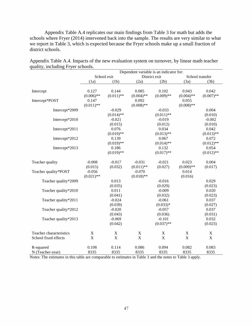
47

Appendix Table A.4 replicates our main findings from Table 3 for math but adds the

schools where Fryer (2014) intervened back into the sample. The results are very similar to what

we report in Table 3, which is expected because the Fryer schools make up a small fraction of

district schools.

Appendix Table A.4. Impacts of the new evaluation system on turnover, by linear math teacher

quality, including Fryer schools. Dependent variable is an indicator for:

School exit District exit School transfer

(1a) (1b) (2a) (2b) (3a) (3b)

Intercept 0.127

(0.006)**

0.144

(0.011)**

0.085

(0.004)**

0.102

(0.009)**

0.043

(0.004)**

0.042

(0.007)**

Intercept*POST 0.147

(0.011)**

0.092

(0.008)**

0.055

(0.008)**

Intercept*2009 -0.029

(0.014)**

-0.033

(0.011)**

0.004

(0.010)

Intercept*2010 -0.021

(0.015)

-0.019

(0.012)

-0.002

(0.010)

Intercept*2011 0.076

(0.019)**

0.034

(0.013)**

0.042

(0.013)**

Intercept*2012 0.139

(0.019)**

0.067

(0.014)**

0.072

(0.012)**

Intercept*2013 0.186

(0.019)**

0.132

(0.017)**

0.054

(0.012)**

Teacher quality -0.008

(0.015)

-0.017

(0.032)

-0.031

(0.011)**

-0.021

(0.027)

0.023

(0.009)**

0.004

(0.017)

Teacher quality*POST -0.056

(0.021)**

-0.070

(0.018)**

0.014

(0.016)

Teacher quality*2009 0.013

(0.035)

-0.016

(0.029)

0.029

(0.023)

Teacher quality*2010 0.011

(0.041)

-0.009

(0.032)

0.020

(0.023)

Teacher quality*2011 -0.024

(0.039)

-0.061

(0.033)*

0.037

(0.027)

Teacher quality*2012 -0.020

(0.043)

-0.057

(0.036)

0.037

(0.031)

Teacher quality*2013 -0.069

(0.042)

-0.101

(0.037)**

0.032

(0.023)

Teacher characteristics X X X X X X

School fixed effects X X X X X X

R-squared 0.108 0.114 0.086 0.094 0.082 0.083

N (Teacher-year) 8335 8335 8335 8335 8335 8335

Notes: The estimates in this table are comparable to estimates in Table 3 and the notes to Table 3 apply.