The Complexity of Planar GraphIsomorphism

Jacobo Torán and Fabian Wagner∗

Abstract

The Graph Isomorphism problem restricted toplanar graphs has beenknown to be solvable in polynomial time many years ago. In terms of com-plexity classes however, the exact complexity of the problem has been estab-lished only very recently. It was proved in [?] that planar graph isomorphismcan be computed within logarithmic space. Since there is a matching hard-ness result [?], this shows that the problem is complete forL. Although thiscould be considered a result in in algorithmics its proof relies on severalimportant new developments in the area of logarithmic spacecomplexityclasses and reflects the close connections between algorithms and complex-ity theory. In this column we give an overview of this result mentioning thedevelopments that led to it.

1 Introduction

The Graph Isomorphism problem asks whether two given graphsare isomorphicor in other words whether there is a bijection between the nodes of the two graphs,preserving the adjacency relation. Graph Isomorphism is one of the few problemsin NP that is not know to be inP or NP-complete. On the other hand, for manyrestricted graph classes like trees, graphs of bounded degree or partialk-trees, ef-ficient algorithms for the isomorphism problem are known. Weconsider in thiscolumn the class of planar graphs and for simplicity restrict ourselves to undi-rected simple graphs. A graph is planar if it can be drawn in the plane withoutany crossing edges. A special class of planar graphs is that of 3-connected planargraphs. A graph isk-connected if it remains connected after deletingk arbitraryvertices. It was shown in 1933 that 3-connected planar graphs have exactly twoplanar embeddings [?]. This fact was used by Weinberg in 1966 to give anO(n2)algorithm for testing isomorphism of 3-connected planar graphs [?] (n is the num-ber of vertices of the input graphs). The idea of the algorithm is simple, the two

∗Universität Ulm, Institut für Theoretische Informatik, fabian.wagner@uni-ulm.de

given graphs are embedded in the plane and it is tested whether the embeddingof the first graph is isomorphic to one of the two possible embeddings of thesecond graph. With this method it is also possible to efficiently assign codes to3-connected planar graphs as a way to identify them. This means that there is anefficiently computable function mapping graphs to strings or codes, so that twographs are mapped to the same code if and only if they are isomorphic. Hopcroftand Tarjan extended Weinberg’s algorithm and gave the first polynomial time al-gorithm for the isomorphism of planar graphs [?]. In their algorithm the graphsare divided first in connected components, these are subdivided in biconnectedcomponents and finally these components are partitioned in 3-connected compo-nents. An initial connected component has articulation points separating its bi-connected components from each other. These initial components are representedby a tree-like structure containing vertices for articulation points and vertices forbiconnected components. In a similar way, the biconnected components are rep-resented by tree structures containing vertices for its 3-connected components andvertices for pairs of nodes (called separating pairs) separating these components.Each vertex representing a 3-connected component is then labeled with the codeof the component and the whole structure can then be tested for isomorphism ina similar way as it is done for tree isomorphism. The originalalgorithm had arunning time ofO(n2). This was then improved toO(n logn) in [?] and finallyHopcroft and Wang [?] obtained a linear time algorithm for the isomorphism ofplanar graphs. Recently Kukluk, Holder, and Cook [?] gave anO(n2) algorithmfor planar graph isomorphism, which is suitable for practical applications.

Regarding the parallel complexity of the problem, Miller and Reif [?] gavethe firstNC algorithm for planar graph isomorphism. Their algorithm runs in timeO(logn) with polynomial number of processors in the CRCW PRAM model. Thiscorresponds to the complexity classAC1 of problems computable by unboundedfan-in circuits of polynomial size and logarithmic depth. More recently, using acompletely different approach based on descriptive complexity, Grohe and Ver-bitski [?] provided a new method for testing isomorphism of planar graphs alsowithin AC1. They proved that for a class G of graphs, if every graph is theclassis definable in first order logic with a finite number of variables and logarithmicquantifier depth, then the isomorphism problem for G is inAC1. Verbitski [?]showed that the class of planar 3-connected graphs is definable with 15 variablesand logarithmic quantifier depth. Together with theAC1 reduction from planarisomorphism to 3-connected planar isomorphism from [?] this provides a differ-ent way to show that planar isomorphism lies inAC1.

We describe in this survey some of the results leading to the improvement ofthe upper bound fromAC1 to logarithmic space. Located betweenL andAC1,the complexity classUL played an important part in the development of the re-sults. UL (unambiguous logarithmic space) is the class of problems computable

by a logarithmic space nondeterministic machine having at most one acceptingcomputation path for each input. The relation between the considered complexityclasses is as follows:

L ⊆ UL ⊆ AC1.

We denote byFL the class of functions computable within logarithmic space.All the isomorphism results described in this overview can in fact be extended

to graph canonization results. For a class G of graphs we say that a functionf : G → {0, 1}∗ computes acomplete invariant for the class if for everyG,H ∈ Git holds thatG andH are isomorphic if and only iff (G) = f (H). If moreover fcomputes for eachG a graphf (G) isomorphic toG then we callf a canonizingfunction and f (G) a canon.

We recall in Section 2 several facts that were used in the proof of the results.Similarly as in the developments leading to polynomial timetest for planar graphisomorphism, the first logarithmic space isomorphism algorithms worked for treesand 3-connected graphs. These are overviewed in Sections 2 and 3. Finally thelogarithmic space algorithm for planar graph isomorphism is explained in Sec-tion 4.

2 Some previous results

2.1 Tree isomorphism in L

Lindell gave in [?] a logarithmic space algorithm for tree isomorphism and can-onization. Some of the ideas in this algorithm are used also in the new results.Lindell defined a canonical ordering between trees. For a tree T , we represent itsroot by t and the out-degree oft by #t. The tree isomorphism ordering<T fromLindell is defined in the following way: Given two treesS andT , we sayS <T Tif:

i) |S | < |T | or

ii) |S | = |T | and #s < #t, or

iii) |S | = |T |, #s = #t = k and (S 1, . . . , S k) < (T1, . . . , Tk) lexicographically, wereS 1 6T S 2, . . . 6T S k, andT1 6T T2 . . . 6T Tk, are the ordered subtrees ofSandT rooted at the children ofs andt.

It is not hard to see that if neitherS <T T nor T <S S then S and T areisomorphic. Obviously the first two tests in the definition oftree ordering can bedone in logarithmic space. Lindell proved that this is also true for the third step.This is done with the following variant of depth first search:

• Find the number of children ofs and t of minimal size. If these numbers donot coincide then declare the tree with the largest number ofminimal sizechildren to be smaller. Otherwise check the next child size until an equalityis found or all the children have been considered.

• If s and t have the same number of children of each size, we partition thechildren into size classes and compare the children in each size class inincreasing order of the sizes recursively as follows: Letk be the number ofchildren in one size class. We can supposek > 0.

– If k = 1 then only one recursive call is made and no extra space is neededfor this.

– If k > 1 then for each node in the size class inS we compute its order pro-file. This consists of three countersc<, c> andc= indicating the num-ber of children in the corresponding size class ofT being respectivelysmaller than, larger than or equal to the node under consideration. Thecounters are updated by making cross comparisons. We start with thechildren with minimal order profile, those with>c= 0. They form anisomorphism class. The size of this class is compared acrossthe treesby comparing the values of thec= counters. If they match, both treeshave the same number of minimal children. To compare larger chil-dren in the same size class, the value ofc= in the last step works asa threshold. This is used to search for the next minimal children of sandt . The process is then repeated and the threshold is incrementeduntil reachingk, at which point we proceed to the next size class. Ifall the size classed are visited without detecting an inequality the treesare isomorphic.

2.2 Planarity testing and distance computation

A graph is planar if it can be drawn on the plane so that no edgescross. Such adrawing is a planar embedding. Allender and Mahajan [?] showed that the prob-lem of determining if a given graph is planar, can be computedin the complexityclassSL (symmetric logarithmic space). Some year later Reingold [?] proved thatthe classedSL andL coincide, thus bringing the planarity recognition problemtoL.

A rotation scheme for a graphG is a setρ of permutations,ρ = {ρv | v ∈ V},whereρv is a permutation onEv that has only one cycle (which is called arotation).Let ρ−1 be the set of inverse rotations,ρ−1

= {ρ−1v | v ∈ V}. A rotation schemeρ

describes an embedding of graphG in the plane. If the embedding is planar,we call ρ a planar rotation scheme. The pair (G, ρ) is called acombinatorial

embedding for G. The planarity recognition result Allender and Mahajan alsoshowed the following useful result:

Theorem 2.1. [?] There is a logarithmic space algorithm that on input a planargraph G produces a planar rotation scheme ρ for G.

A planar 3-connected graph has exactly two planar rotation schemes [?], somerotationρ and its inverseρ−1.

An important tool in one the the isomorphism test for 3-connected planargraphs is the computation of the distances in planar graphs within the classUL:

Theorem 2.2. [?] The distance between two given vertices in a planar graph canbe computed in UL ∩ coUL.

This theorem builds on a series of results dealing with the reachability problemin directed planar graphs, [?],[?] that lead to an algorithm from Bourke, Tewariand Vinodchandran [?] to compute the reachability problem for planar graphswithin UL ∩ coUL.

2.3 Universal exploration sequences

The celebrated result from Reingold [?] showing that the reachability problem inundirected graphs can be computed inL, has an important consequence for theconstruction of universal exploration sequences in logarithmic space. This fact isused in some of the isomorphism algorithms.

For ad-regularG and a numbering of the edges, and an starting edgee0, asequence (τ1, τ2, . . . , τl) ∈ {0, . . . , d − 1}l defines a walkv−1, v0, . . . , vk in G in thefollowing way: starting ate0 = (v−1, v0) for eachi, if (vi−1, vi) is thek-th edge ofvithen (vi, vi+1) is thek + τi edge ofvi modulod.

A sequence (τ1, τ2, . . . , τl) ∈ {0, . . . , d − 1}l is called an (n, d) universal explo-ration sequence n if for every connectedd-regular graph with at mostn vertices,any numbering of its edges and any starting edge, the walk obtained from thesequence explores all the vertices in the graph.

The result that we use is that such universal exploration sequences exist andcan be computed in logarithmic space.

Theorem 2.3. [?] There exists a logarithmic space algorithm that on input (1n, 1d)produces an (n, d)-universal exploration sequence of polynomial size.

3 Planar 3-connected Graph Isomorphism

Weinberg’s [?] O(n2) algorithm for testing isomorphism of planar 3-connectedgraphs constructs a code for every edge ofG and both rotation schemes. Of all

these codes, the lexicographical smallest one is used as a canonical form forG.Weinberg’s algorithm does not work within logspace, because the vertices andedges have to be stored. Thierauf and Wagner showed in [?] how to constructa different code inUL. Some months later, using Reingolds results on logarith-mic space universal exploration sequences [?], Datta, Limaye and Nimbhorkarimproved this to an isomorphism algorithm for planar 3-connected graphs thatworks in logarithmic space. We describe both results in thissection.

3.1 An isomorphism algorithm in UL ∩ coUL

Theorem 3.1. [?] The isomorphism problem for planar, 3-connected graphs is inUL ∩ coUL.

Let (s, t) be a designated edge andρ be a rotation scheme forG. The con-struction has three steps: First, we compute a canonical spanning treeT for G.Second, with help of this spanning tree and the rotation function ρ we perform adepth-first traversal on the edges of the graph and constructa canonical listL ofall edges ofG. Finally, we rename the vertices depending on the position of theirfirst occurrence in the listL.

We will see that the spanning tree in step 1 can be computed in (the functionalversion of)UL ∩ coUL. The list and the renaming in step 2 and step 3 can becomputed inFL.

The overall algorithm has to decide whether two given graphsG andH areisomorphic. To do so we fix (s, t) andρ for G and cycle through all edges ofHas designated edge and the two possible embeddings ofH. ThenG and H areisomorphic if and only if the canonical forms forG andH match. It is not hard tosee that this outer loop works in logspace.

Step 1: Construction of a canonical spanning tree

We show that the following problem can be solved in unambiguous logspace.Given, an undirected graphG = (V, E), a rotation schemeρ for G, and a designatededge (s, t) ∈ E. Output a canonical spanning treeT ⊆ E of G, which does notdepend on the input representation ofρ or G, any representation will result in thesame spanning treeT .

The idea to construct the spanning tree is to traverseG with a breadth-firstsearch starting at nodes. The neighbors of a node are visited in the order givenby the rotation schemeρ. Since the algorithm should work in logspace, we cannotafford to store all the nodes that we already visited, as in a standard breadth-firstsearch. We get around this problem by working with distancesbetween nodes.

We start with the nodes at distance 1 froms. That is, write (s, v) on the outputtape, for allv ∈ Γ(s). Now let d > 2 and assume that we have already con-structedT up to nodes at distance6 d − 1 to s. Then we consider the nodes atdistanced from s. Let w be a node withd(s, w) = d. We connectw to the treeconstructed so far by computing a shortest path froms to w. Ambiguities are re-solved by using the first feasible edge according toρ. We start with (s, t) as theactive edge (u, v).

• If d(u, w) > d(v, w), then (u, v) is the first edge encountered that is on ashortest path fromu to w. Therefore we go fromu to v and start searchingthe next edge fromv. As starting edge we takeρv(v, u), the successor of(v, u). It is the new active edge.

• If d(u, w) 6 d(v, w), then (u, v) is not on a shortest path fromu to w. Thenwe proceed withρu(u, v) as the new active edge.

After d − 1 steps in direction ofw, the nodev of the active edge (u, v) is a pre-decessor ofw on a shortest path froms to w. Then we write (v, w) on the outputtape.

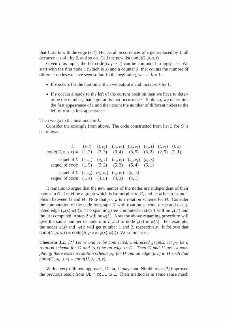
The spanning treeT is canonical, because its construction depends only onρ,edge (s, t), and edge setE. The following figure shows an example of a spanningtreeT for a graphG with rotation functionρwhich arranges the edges in clockwiseorder around each vertex.

ρv3

ρv2

ρv1

ρt

= ( (s, t) (s, v1) (s, v2) )= ( (t, s) (t, v3) (t, v1) )= ( (v1, s) (v1, t) (v1, v3) (v1, v2) )= ( (v2, s) (v2, v1) (v2, v3) )= ( (v3, t) (v3, v2) (v3, v1) )

ρs

ρ = {ρs, ρt, ρv1, ρv2, ρv3}

v1

v3

t

s

v2

Except for the computation of the distances, the algorithm works in logspace.We have to store the values ofd, k, u and v, and the position ofw, plus someextra space for doing calculations. By Theorem?? above, the distances can becomputed inUL∩coUL. SinceLUL∩coUL

= UL∩coUL the canonical spanning treecan be computed inUL ∩ coUL.

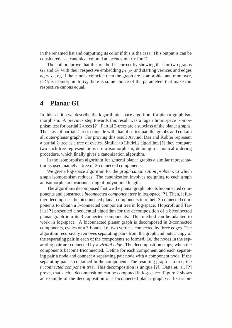
(s, v2)(v2, v1)(v2, v3)(v2, s)

(s, v1)(v1, t)(v1, v3)(v1, v2)(v1, s)

(s, t)(t, v3)(v3, v2)(v3, v1)(v3, t)(t, v1)(t, s)L =

v1

v3

t

s

v2

Figure 1: Computation of ListL for G.

Step 2: Computation of a canonical list of all edges

With G = (V, E), a rotation schemeρ for G, a spanning treeT ⊆ E of G, and adesignated edge (s, t) ∈ T we compute a canonical listL of all edges inE. The listL then still contains the original vertex names inG, it does not depend otherwiseon the input representation ofρ, G or T .

The idea is to traverse the spanning tree in a depth-first manner. At eachvertexu we visit all incident edges ofu in a cyclic manner according toρu untilthe next edgee of the spanning tree is reached. We go down the tree alonge andrecursively do the same at the node reached. At some point we will encountereagain and come back tou. Then we continue to output the edges incident tou.

More formally, we start the traversal with edge (s, t) as the active edge (u, v).We write (u, v) on the output tape and then compute the next active edge as follows:

• If (u, v) ∈ T then we walk depth-first inT from u to v, consider the edge(v, u) and takeρv(v, u) its successor according toρv.

• If (u, v) < T then we proceed breadth-first withρu(u, v).

This step is repeated until we entirely traversedE and the active edge is again(s, t). Every undirected edge is encountered exactly once in eachdirection.

The following figure shows an example forL.

Step 3: Renaming the vertices

The last step is to rename the vertices in the listL such that they become inde-pendent of the names they have inG. This is achieved as follows: consider thefirst occurrence (from left) of nodev in L. Let k − 1 be the number of pairwisedifferent nodes to the left ofv. Then all occurrences ofv are replaced byk. Recall,

thatL starts with the edge (s, t). Hence, all occurrences ofs get replaced by 1, alloccurrences oft by 2, and so on. Call the new listcode(G, ρ, s, t).

Given L as input, the listcode(G, ρ, s, t) can be computed in logspace. Westart with the first nodev (which is s) and a counterk, that counts the number ofdifferent nodes we have seen so far. In the beginning, we setk = 1.

• If v occurs for the first time, then we outputk and increasek by 1.

• If v occurs already to the left of the current position then we have to deter-mine the number, thatv got at its first occurrence. To do so, we determinethe first appearance ofv and then count the number of different nodes to theleft of v at its first appearance.

Then we go to the next node inL.Consider the example from above. The code constructed from list L for G is

as follows.

L = (s, t) (t, v3) (v3, v2) (v3, v1) (v3, t) (t, v1) (t, s)code(G, ρ, s, t) = (1, 2) (2, 3) (3, 4) (3, 5) (3, 2) (2, 5) (2, 1)

sequel ofL (s, v1) (v1, t) (v1, v3) (v1, v2) (v1, s)sequel ofcode (1, 5) (5, 2) (5, 3) (5, 4) (5, 1)

sequel ofL (s, v2) (v2, v1) (v2, v3) (v2, s)sequel ofcode (1, 4) (4, 5) (4, 3) (4, 1)

It remains to argue that the new names of the nodes are independent of theirnames inG. Let H be a graph which is isomorphic toG, and letϕ be an isomor-phism betweenG andH. Note thatρ ◦ ϕ is a rotation scheme forH. Considerthe computation of the code for graphH with rotation schemeρ ◦ ϕ and desig-nated edge (ϕ(s), ϕ(t)). The spanning tree computed in step 1 will beϕ(T ) andthe list computed in step 2 will beϕ(L). Now the above renaming procedure willgive the same number to nodev in L and to nodeϕ(v) in ϕ(L). For example,the nodesϕ(s) and ϕ(t) will get number 1 and 2, respectively. It follows thatcode(G, ρ, s, t) = code(H, ρ ◦ ϕ, ϕ(s), ϕ(t)). We summarize:

Theorem 3.2. [?] Let G and H be connected, undirected graphs, let ρG be arotation scheme for G and (s, t) be an edge in G. Then G and H are isomor-phic iff there exists a rotation scheme ρH for H and an edge (u, v) in H such thatcode(G, ρG, s, t) = code(H, ρH, u, v).

With a very different approach, Datta, Limaye and Nimbhorkar [?] improvedthe previous result fromUL ∩ coUL to L. Their method is in some sense much

easier since it avoids the spanning tree construction eliminating the distance com-putations (the part inUL∩ coUL). It uses however the concept of universal explo-ration sequence and the non-trivial fact that such sequences can be computed inL.

Theorem 3.3. [?] The isomorphism problem for planar, 3-connected graphs is inL.

The idea of the algorithm is to use a universal sequence [?] in order to con-struct a canonical code for a given planar 3-connected graphG. Since Reingolds’sconstruction requires the graph to have constant degree, there is a proprocesingstep in whichG is transformed into a 3-regular colored graphG′ with the prop-erty that two graphs are isomorphic if and only if their transformations are alsoisomorphic (with a color preserving isomorphism). In a second step a canonicalcode is computed. The code is specific to the choice of a planarembeddingρ forG, a starting node and a starting edge. Since there are only polynomially manypossible choices for these parameters, for two given graphsG andH, a logarithmicspace procedure can cycle through all the possibilities anddecide that the graphsare isomorphic if and only if the canonical codes match for any of the choices.

Step 1: Making the graph 3-regular

Given a 3-connected planar graphG = (V, E) and a planar embeddingρ we con-struct a 3-regular planar graphG′ with the edges colored with two colors.G′

might not be 3-connected, however the planar embedding fromG will be inher-ited toG′. Every vertexv of G is replaced inG′ by a cycle{v1, . . . , vd} (d is thedegree ofv). Thed edgese1, . . . , ed incident withv in G are now respectively inci-dent to{v1, . . . , vd} in G′. The cycles edges are colored with color 1 and the edgese1, . . . , ed with color 2. The obtained graphG′ is 3-regular and it is not hard to seethat two graphsG andH are isomorphic if and only if their transformationG′ andH′ are isomorphic with a color preserving isomorphism.

Step 2: Obtaining the canonical code

On input an edge-colored graphG with n vertices, max. degree 3, a planar em-beddingρ a starting vertexv and a starting edgee = (u, v), a cannon forG isconstructed. For this we compute first in logarithmic space a(n, 3)-universal ex-ploration sequenceU. Then, starting atv ande we transverseG according toUandρ giving the listL of the visited vertices as label. We can rename the verticesaccording to their first occurrence inL, as it is done in step 3 from Theorem 3.1.Finally we can cycle over every possible pair (i, j) checking whether it is an edge

in the renamed list and outputting its color if this is the case. This output is can beconsidered as a canonical colored adjacency matrix forG.

The authors prove that this method is correct by showing thatfor two graphsG1 andG2 with their respective embeddingρ1, ρ2 and starting vertices and edgesv1, v2, e1, e2, if the canons coincide then the graph are isomorphic, and moreover,if Gi is isomorphic toG2 there is some choice of the parameters that make thirrespective canons equal.

4 Planar GI

In this section we describe the logarithmic space algorithmfor planar graph iso-morphism. A previous step towards this result was a logarithmic space isomor-phism test for partial 2-trees [?]. Partial 2-trees are a subclass of the planar graphs.The class of partial 2-trees coincide with that of series-parallel graphs and containall outer-planar graphs. For proving this result Arvind, Das and Köbler representa partial 2-tree as a tree of cycles. Similar to Lindells algorithm [?] they comparetwo such tree representations up to isomorphism, defining a canonical orderingprocedure, which finally gives a canonization algorithm.

In the isomorphism algorithm for general planar graphs a similar representa-tion is used, namely a tree of 3-connected components.

We give a log-space algorithm for thegraph canonization problem, to whichgraph isomorphism reduces. The canonization involves assigning to each graphan isomorphism invariant string of polynomial length.

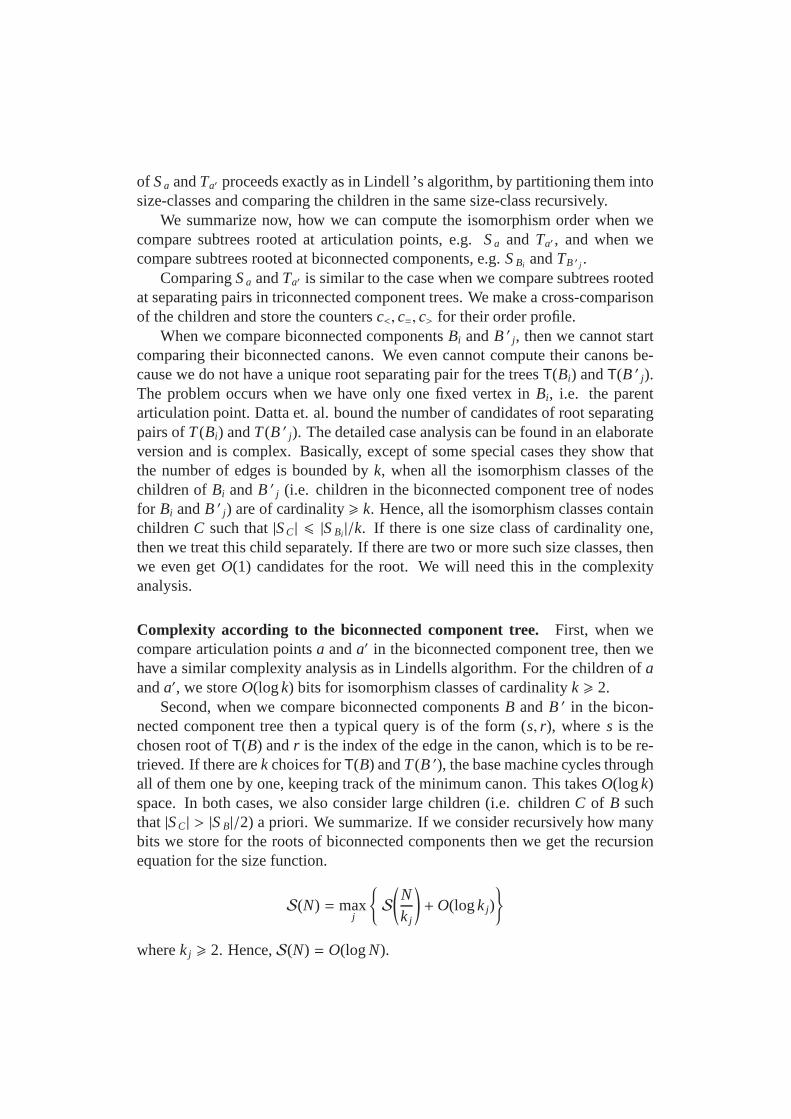
The algorithms decomposed first we the planar graph into its biconnected com-ponents and construct abiconnected component tree in log-space [?]. Then, it fur-ther decomposes the biconnected planar components into their 3-connected com-ponents to obtain a 3-connected component tree in log-space. Hopcroft and Tar-jan [?] presented a sequential algorithm for the decomposition ofa biconnectedplanar graph into its 3-connected components. This method can be adapted towork in log-space. A biconnected planar graph is decomposedin 3-connectedcomponents, cycles or a 3-bonds, i.e. two vertices connected by three edges. Thealgorithm recursively removes separating pairs from the graph and puts a copy ofthe separating pair in each of the components so formed, i.e.the nodes in the sep-arating pair are connected by avirtual edge. The decomposition stops, when thecomponents become triconnected. Define for each component and each separat-ing pair a node and connect a separating pair node with a component node, if theseparating pair is contained in the component. The resulting graph is a tree, thetriconnected component tree. This decomposition is unique [?]. Datta et. al. [?]prove, that such a decomposition can be computed in log-space. Figure 2 showsan example of the decomposition of a biconnected planar graph G. Its tricon-

nected components areG1, . . . ,G4 and the corresponding triconnected componenttree isT . In G, the pairs (a, b) and (c, d) are the separating pairs. Since the 3-connected separating pair (c, d) is connected by an edge inG, we also get{c, d} astriple-bondG3. The virtual edges corresponding to the separating pairs are drawnwith dashed lines.

f b e

c

dd

b

a

a

c

G1

bfa

d

G2

G4

b

c

d

a e

c

d

G4G2G3G

G1 T

G3

c

Figure 2:Decomposition of a biconnected planar graph into a triconnected com-ponent tree.

The triconnected components can be canonized in log-space [?]. Hence, fortriconnected component trees, compute their canonical invariant in log-space, i.e.two biconnected graphs are isomorphic if their trees are found to be equal.

In section 4.0.1, we summarize, how to canonize biconnectedplanar graphs byapplying tree canonization ideas from [?] to their triconnected component trees.Note that, pairwise isomorphism of two trees labelled with the canons of theircomponents does not imply isomorphism of the correspondinggraphs. Lindell ’salgorithm and complexity analysis had to be modified in a non-trivial way for thisstep to work in log-space.

In section 4.0.2, we describe, how to canonize planar graphsusing their bicon-nected component trees, again, using the basic structure ofLindell ’s algorithm.The comparison algorithm refers to the biconnected component tree of the planargraph and when comparing biconnected components, to their triconnected com-ponent trees. This requires a detailed analysis of the interferences of both treestructures.

4.0.1 Canonization of biconnected planar graphs

Let S and T be two triconnected component trees for the biconnected planargraphsG andH, respectively.S andT are rooted at separating pair nodes, says = (a, b) andt = (a′, b ′). Therefore we also writeS (a,b) andT(a′ ,b ′). They haveseparating pair nodes at odd levels and triconnected component nodes at evenlevels. Figure 3 shows two trees to be compared.

bas

G1

. . .

. . .. . .

. . . Gk

s1

. . . . . .

. . .. . .

. . .

. . .

ta′ b′

HkH1

t1slk tlksl1 tl1

S (a,b) T(a′ ,b′)

S 1 S lk T1 Tlk

S G1 S Gk THkTH1

Figure 3: Triconnected component trees.

Similar as in Lindells algorithm, we define the isomorphism order of two tri-connected component treesS and T rooted at separating pairss = (a, b) andt = (a′, b ′). S (a,b) <T T(a′,b ′) if:

1. |S (a,b)| < |T(a′,b ′)| or

2. |S (a,b)| = |T(a′,b ′)| but #s < #t or

3. |S (a,b)| = |T(a′ ,b ′)|, #s = #t = k, but (S G1, . . . , S Gk) <T (TH1, . . . , THk) lexico-graphically, where we assume thatS G1 6T . . . 6T S Gk andTH1 6T . . . 6T THk

are the ordered subtrees ofS (a,b) andT(a′,b ′), respectively. To compute theorder between the subtreesS Gi andTHi we compare lexicographically thecanons ofGi andHi andrecursively the subtrees rooted at the children ofGi

andHi. Note that these children are again separating pair nodes.

4. |S (a,b)| = |T(a′ ,b ′)|, #s = #t = k, (S G1 6T . . . 6T S Gk) =T (TH1 6T . . . 6T THk),but (O1, . . . ,Op) < (O ′

1, . . . ,O ′p) lexicographically, whereO j and O ′

j

are the orientation counters of thejth isomorphism classesI j and I′j of alltheS Gi ’s and theTHi ’s.

We say that two triconnected component treesS e andTe′ areequal accord-ing to the isomorphism order, denoted byS e =T Te′ , if neither S e <T Te′ norTe′ <T S e holds. Two trees are=T-equal, precisely when the underlying graphs areisomorphic.

We summarize now, how we can compute the isomorphism order when wecompare subtrees rooted at separating pairs, e.g.S (a,b) andT(a′,b ′), and when wecompare subtrees rooted at triconnected components, e.g.S Gi andTH j .

ComparingS (a,b) andT(a′,b′) is similar to the comparison of subtrees in Lindellsalgorithm. We make a cross-comparison of the children and store the countersc<, c=, c> for their order profile.

Assume, both subtrees are of equal size, i.e.|S Gi | = |TH j | = N, both rooted attriconnected component nodesGi andH j, respectively.

First, we compare the types ofGi andH j. We say that bonds6T cycles and cy-cles6T 3-connected components. 3-bonds are always equal. If both are cycles or3-connected components then we construct the canons ofGi andH j and compareall of them bit-by-bit.

To canonize a cycle, we traverse it starting from the virtualedge which cor-responds to its parent (i.e. the parent node ofGi), and then traversing the entirecycle along the edges encountered. There are two possible traversals dependingon which direction of the starting edge is chosen. Thus, a cycle has two possiblecanons.

To canonize a 3-connected componentGi, we use the log-space algorithmfrom Datta, Limaye, and Nimbhorkar [?]. The canon depends on the direction ofthe starting edge and additionally, on the embedding of the componentGi. For3-connected components, there are two possible embeddings. Hence, we have upto four possible canons.

In the bit-by-bit comparison, we have to distinguish several cases. When wereach virtual edges in the comparison steps, we go into recursion at the subtreesrooted at the corresponding separating pairs. If we find in the recursion that one ofthe subtrees is smaller than the other, then we have found an inequality betweenthe current canons we compare. We eliminate the canons whichare not found tobe minimal. At the end, if there remains a canon forGi and for H j, then bothsubtreesS Gi andTH j are equal up to step 3.

Orientation counters. However, here it does not suffice to stop after step 3. Weneed a further comparison step to ensure thatG and H are indeed isomorphic.To see this we give an example, consider Figure 4. Assume thats and t havetwo children each,G1, G2 and H1, H2 such thatG1 � H1 andG2 � H2. Stillwe cannot conclude thatG andH are isomorphic because it is possible that theisomorphism betweenG1 andH1 mapsa to a′ andb to b ′, but the isomorphismbetweenG2 andH2 mapsa to b ′ andb to a′. Then these two isomorphisms cannotbe extended to an isomorphism betweenG andH.

To handle this problem, we introduce the notion of anorientation of a sep-arating pair. A separating pair gets an orientation from subtrees rootedat itschildren. Also, every subtree rooted at a triconnected component node gives anorientation to the parent separating pair. If the orientation is consistent, then wedefineS (a,b) =T T(a′,b ′) and we will show thatG andH are isomorphic in this case.

b′a

G

b′b

Ha

a′

b

b′

b

a′

a

a′

b′

a

b′a′ a′

bG1 G2

a

H2

b

H1

G0

S (a,b)

H0

T(a′,b′)

Figure 4:

We define theorientation given to the parent separating pair of Gi andH j asthe direction in which the minimum canon traverses this edge. If the minimumcanons are obtained for both choices of directions of the edge, we say thatS Gi

andTH j aresymmetric about their parent separating pair, and thus do not give anorientation.

We define theorientation given to the virtual edge in the parent tricon-nected component of the corresponding separating pair node (a, b) or (a′, b ′)by considering all the orientations given to the separatingpair of their childrenG1, . . . ,Gk, respectively. We first order the subtrees, sayS G1 6T · · · 6T S Gk andTH1 6T · · · 6T THk , and partition them into isomorphism classes, sayI1, . . . , Ip

andI′1, . . . , I′p. Let I j be the smallest isomorphism class such that there are more

components that give the orientationa → b to the parent thanb → a (or viceversa). Then, we definea → b to be thereference orientation (b → a other-wise). For each isomorphism classI j, we compute now the orientation countersO j = (c→j , c

←j ) such thatc→j is the number of children inI j which give the ref-

erence orientation andc←j is the number of children inI j which give the reverseorientation.

Recall the example of Figure 4. The graphsG andH have the same tricon-nected component trees but are not isomorphic. InS (a,b), the 3-bonds form oneisomorphism classI1 and the other two components form the second isomorphismclassI2, as they all are pairwise isomorphic. The non-isomorphism is detected bycomparing the directions given to the parent separating pair. We havep = 2 iso-morphism classes and for the orientation counters we haveO1 = O ′

1 = (0, 0),whereasO2 = (2, 0) andO ′

2 = (1, 1) and henceO ′2 is lexicographically smaller

thanO2. Therefore we haveT(a′,b ′) <T S (a,b).

Complexity. We argue now, that we can do the four comparison steps in log-space. The first and the second step are similar to Lindells algorithm. We define

the size of a separating pair node as 2 and the size of a triconnected component asthe number of vertices in the component. For the third and fourth step, we havethe following cases:

• When we compare two triconnected componentsGi andH j, then we haveup to four canons. Suppose, we construct and compare two canonsCg andCh and reach separating pairs (a, b) and (a′, b ′). We store the canons whichare not eliminated, which of themCg andCh are and the direction of thevirtual edges (a, b) and (a′, b ′). Hence, we needO(1) bits.

• When we compare two separating pairs (a, b) and (a′, b ′), then we makea cross-comparison as in Lindells algorithm. Hence, we needcountersc<, c=, c> to store the order profile. This way, we get the isomorphismclasses. We further store the orientation countersO j and O ′

j for I j andI′j. We needO(log |I j|) bits on the work-tape for all the counters.

However, we cannot guarantee yet, that the algorithm works in log-space. LetS C be the subtree rooted at nodeC in a triconnected component tree. The problemis, that the subtrees (i.e. the children ofC) where we go into recursion might beof size> |S C |/2, we call it alarge child.

To get around this problem, we first check whether the nodesC andC ′ havea large child. If so, then we compare them a priori and store the result of theircomparison and the orientation given to the parent. BecauseC andC ′ have atmost one large child, this needs onlyO(1) additional bits. Whenever we would gointo recursion at those large children, we just look at the work-tape for the result.

As seen above, while comparing two trees of sizeN, the algorithm uses nospace for making a recursive call for a subtree of size largerthanN/2, and it usesO(logk j) space if the subtrees are of size at mostN/k j, wherek j > 2. Hence weget the same recurrence for the spaceS(N) as Lindell:

S(N) 6 maxjS

(Nk j

)+ O(logk j),

wherek j > 2 for all j. ThusS(N) = O(logN). Note that the numbern of nodesof G is in general smaller thanN, because the separating pair nodes occur in allcomponents split off by this pair. But we certainly haven < N 6 O(n2) [?]. Thisproves the following theorem.

Theorem 4.1. The isomorphism order between two triconnected component treesof biconnected planar graphs can be computed in log-space.

The canon. Once we know the ordering among the subtrees, it is straight for-ward to output the canon of the triconnected component treeT . We traverseT inthe tree isomorphism order as in Lindell [?], outputting the canon of each of thenodes along with virtual edges and delimiters. That is, we output a ‘[’ while goingdown a subtree, and ‘]’ while going up a subtree.

We need to choose a separating pair as root for the tree. Sincethere is nodistinguished separating pair, we simply cycle through allof them and select theone, which leads to the minimum canon. Let (a, b) be this separating pair.

The canonization procedure has two steps. In the first step wecompute whatwe call acanonical list for S (a,b). This is a list of the edges ofG, also includingvirtual edges. In the second step we compute the final canon from the canonicallist.Canon of separating pair nodes. Consider a subtreeS (a,b) rooted at (a, b). Westart with computing the reference orientation of (a, b) with oracle calls to thecanonical ordering algorithm and output the edge in this direction. Then we re-cursively output the canonical lists of the subtrees of node(a, b) according to theincreasing isomorphism order. Among isomorphic siblings,those which give thereference orientation to the parent come first. We denote this canonical list ofedgesl(S , a, b). If there is no reference orientation for a child, take the orientationof the parent (a, b).Canon of triconnected component nodes. Consider the subtreeS Gi rooted atGi.Let (a, b) be the parent separating pair ofS Gi with reference orientation (a, b).If Gi is a 3-bond then outputl(Gi, a, b) = (a, b). If Gi is a cycle then outputl(Gi, a, b) = (a, b)(b, v1)(v1, v2) . . . (vn, b). If Gi is a 3-connected component thencompute the minimum of two canons with an oracle call, with respect to the givenreference orientation (a, b) and both embeddings forGi. Output this canon asl(Gi, a, b). Virtual edges are output in the direction of the referenceorientationgiven to them, if any. Finally, we output the subtrees in the order we have virtualedges in the canon.

We give now an example. Consider the canonical listl(S , a, b) of edges forthe treeS (a,b) of Figure 3. Letsi be the edge connecting the verticesai with bi.We also write for shortl ′(S i, si) which is one ofl(S i, ai, bi) or l(S i, bi, ai). Thedirection ofsi is as described above. Letl0 = 0. Then we have:

l(S , a, b) = [ (a, b) l(S G1, a, b) . . . l(S Gk , a, b) ], where

l(S Gi , a, b) = [ l(Gi, a, b) [l ′(S li−1+1, sli−1+1)] . . . [l ′(S li , sli)] ] ]

4.0.2 Canonization of planar graphs

Consider the decomposition of a connected planar graph. Foreach articulationpoint and biconnected component we define nodes i.e.articulation point nodes

andbiconnected component nodes. An articulation point node fora is connectedby an edge to the nodes of biconnected components wherea is contained as avertex. The resulting graph is a tree, thebiconnected component tree. The maindifference to the triconnected component tree is, that for articulation point nodes,there is no concept of orientation as for separating pairs.

We define the isomorphism order for two biconnected component treesS a

andTa′ rooted at nodess andt corresponding to articulation pointsa anda′, re-spectively. Also see Figure 5. Let|S a| be the sum of the sizes of the nodes inthe tree. The size of an articulation point nodea is defined as 1 and the size ofa biconnected component nodeB is the size of its triconnected component tree|T(B)|. DefineS a <B Ta′ if

1. |S a| < |Ta′ | or

2. |S a| = |Ta′ | but #s < #t or

3. |S a| = |Ta′ |, #s = #t = k, but (S B1, . . . , S Bk) <B (TB ′1, . . . , TB ′k) lexicograph-ically, where we assume thatS B1 6B · · · 6B S Bk andTB ′1 6B · · · 6B TB ′k

are the ordered subtrees ofS a andTa′ , respectively. To compare the orderbetween the subtreesS Bi andTB ′ j we compare the triconnected componenttreesT(Bi) of Bi andT(B ′ j) of B ′ j and when we reach the first occurrencesof some articulation points then we comparerecursively the correspondingsubtrees rooted at the children ofBi andB ′ j. Note, that these children areagain articulation point nodes.

. . .

. . .

. . .

. . . . . .

. . .

. . .

. . .

. . . . . .

B1 Bk B′1 B′k

a′

a′l1 a′lka′1al1a1 alk

aTa′S a

S a1Ta′1

S alkTa′lk

TB′1TB′kS BkS B1

Figure 5: Biconnected component trees.

We say that two biconnected component trees areequal, denoted byS a =B Ta′ ,if neither ofS a <B Ta′ andTa′ <B S a holds. The inductive ordering of the subtrees

of S a andTa′ proceeds exactly as in Lindell ’s algorithm, by partitioning them intosize-classes and comparing the children in the same size-class recursively.

We summarize now, how we can compute the isomorphism order when wecompare subtrees rooted at articulation points, e.g.S a and Ta′ , and when wecompare subtrees rooted at biconnected components, e.g.S Bi andTB ′ j .

ComparingS a andTa′ is similar to the case when we compare subtrees rootedat separating pairs in triconnected component trees. We make a cross-comparisonof the children and store the countersc<, c=, c> for their order profile.

When we compare biconnected componentsBi andB ′ j, then we cannot startcomparing their biconnected canons. We even cannot computetheir canons be-cause we do not have a unique root separating pair for the trees T(Bi) andT(B ′ j).The problem occurs when we have only one fixed vertex inBi, i.e. the parentarticulation point. Datta et. al. bound the number of candidates of root separatingpairs ofT (Bi) andT (B ′ j). The detailed case analysis can be found in an elaborateversion and is complex. Basically, except of some special cases they show thatthe number of edges is bounded byk, when all the isomorphism classes of thechildren ofBi andB ′ j (i.e. children in the biconnected component tree of nodesfor Bi andB ′ j) are of cardinality> k. Hence, all the isomorphism classes containchildrenC such that|S C | 6 |S Bi |/k. If there is one size class of cardinality one,then we treat this child separately. If there are two or more such size classes, thenwe even getO(1) candidates for the root. We will need this in the complexityanalysis.

Complexity according to the biconnected component tree. First, when wecompare articulation pointsa anda′ in the biconnected component tree, then wehave a similar complexity analysis as in Lindells algorithm. For the children ofaanda′, we storeO(logk) bits for isomorphism classes of cardinalityk > 2.

Second, when we compare biconnected componentsB and B ′ in the bicon-nected component tree then a typical query is of the form (s, r), wheres is thechosen root ofT(B) andr is the index of the edge in the canon, which is to be re-trieved. If there arek choices forT(B) andT (B ′), the base machine cycles throughall of them one by one, keeping track of the minimum canon. This takesO(logk)space. In both cases, we also consider large children (i.e. childrenC of B suchthat |S C | > |S B|/2) a priori. We summarize. If we consider recursively how manybits we store for the roots of biconnected components then weget the recursionequation for the size function.

S(N) = maxj

{S

(Nk j

)+ O(logk j)

}

wherek j > 2. Hence,S(N) = O(logN).

Complexity according to the triconnected component trees. We considernow the comparison of triconnected component treesT(B) andT(B ′) of bicon-nected componentsB andB ′. In the comparison ofT(B) andT(B ′), we still gointo recursion at separating pairs and when we reach virtualedges in canons fortriconnected components. What is new, we go into recursion when we reach ar-ticulation points. For an example, see Figure 6.

a

S B

a

B

u

u

wu

u w

v

v

v

b

b b

ba

uA

s

a a

S a

T(B)

w

Figure 6:A biconnected component treeS B rooted at biconnected componentBwhich has an articulation pointa as child, which occurs in the triconnected com-ponent treeT(B) of B. In A and the other triconnected components the dashededges are separating pairs.

If an articulation pointa belongs to many separating pairs, then it can occur inmany component nodes inT(B). Recall, that we have a root for the tree. So, thereexists a unique componentA that is closest to the root, wherea is contained. Ob-serve, that the set of component nodes wherea is contained is always a connectedsubtree inT(B). The authors show, that this unique component can be computedin log-space and that the first position wherea occurs in the canon ofA can befound in log-space. Exactly there, we go fora into recursion. For all the otheroccurrences ofa we do not go into recursion. Call this thereference copy of a inT(B).

Assume we store the bits separately, which we need insideT(B) for all bicon-nected componentsB. Then we can prove for this part also a log-space bound.

Therefore, we refine the size function. LetC be a node inT(B). The size ofthe subtreeS C rooted at some nodeC is the sum of the size of the triconnectedsubtree rooted atC in T(B), say|S C | plus the size of all the biconnected subtrees|S a|, if a is a reference copy of an articulation points inS C. Hence, we get thesame recursion equation as before. This finishes the complexity analysis. We getthe following theorem.

Theorem 4.2. The isomorphism order between two planar graphs can be com-puted in log-space.

The canon. The canonization of planar graphs proceeds exactly as in thecaseof biconnected planar graphs. A log-space procedure traverses the biconnectedcomponent tree, makes oracle queries to the isomorphism order algorithm andoutputs a canonical list of edges, along with delimiters to separate the lists forsiblings. A log-space transducer then renames the verticesaccording to their firstoccurrence in this list, to get the final canon for the biconnected component tree.This canon depends upon the choice of the root of the biconnected component tree.Further log-space transducers cycle through all the articulation points as roots tofind the minimum canon among them, then rename the vertices according to theirfirst occurrence in the canon and finally, remove the virtual edges and delimitersto obtain a canon for the planar graph. This proves the main theorem.

Theorem 4.3. A planar graph can be canonized in log-space.

References