The Complexity of Entailment Problems overConditional Equality Constraints ?

Zhendong Su∗

Department of Computer Science, University of California, Davis, CA 95616-8562+1 530 7545376 (phone) +1 530 7524767 (fax)

Alexander Aiken

Computer Science Department, Stanford University, Stanford, CA 94305-9025

Abstract

Equality constraints (a.k.a. unification constraints) have widespread use in static programanalysis, most notably in static polymorphic type systems.Conditional equality constraintsextend equality constraints with a weak form of subtyping to allow more accurate analy-ses and more expressive type systems. In this paper, we present a complete complexitycharacterization of the various entailment problems over conditional equality constraints.In particular, as the main result of the paper, we show that restricted entailment (a.k.a. ex-istential entailment) over conditional equality constraints is PTIME-complete. In addition,we study entailment over a natural extension of conditional equality constraints to providea boundary between tractable constraint classes and intractable ones w.r.t. entailment.

Key words: type systems, static analysis, constraints, algorithms, complexity

1 Introduction

There are two decision problems associated with constraints:satisfiabilityanden-tailment. For the commonly used constraint languages in type inference and pro-gram analysis applications, the satisfiability problem is now well understood [AWL94,And94, FFK+96, Hei94, JM79, MW97, PS91, Rey69, Shi88, FF97, FFSA98, SFA00].

? An earlier version [SA01] of the paper was published in the Proceedings of EuropeanSymposium on Programming (ESOP’01), pages 170–189, Genova, Italy, April 2-6 2001.∗ Corresponding author.

Email address:su@cs.ucdavis.edu (Zhendong Su).

Preprint submitted to Elsevier Science 18 December 2003

For example, it is well-known that satisfiability of equality constraints can be de-cided in almost linear time (linear time if no infinite terms are allowed [PW78]).For entailment problems much less is known, and the few existing results give in-tractable lower bounds for the constraint languages they study, except for equalityconstraints where polynomial time algorithms exist [Col82, Col84].

In this paper, we consider entailment problems overconditional equality constraints,which extend the usual equality constraints with an additional form of constraints:α⇒ τ . This constraint is satisfied ifα = ⊥ orα = τ , where⊥ is the usual elementof bottom. Conditional equality constraints have been used in a number of programanalyses, such as the tagging analysis of Henglein [Hen92], the pointer analysisproposed by Steensgaard [Ste96], and a form of equality-based flow systems forhigher order functional languages [Pal98]. We also consider entailment problemsover a natural extension of conditional equality constraints to provide a simple andnatural separation of tractable and intractable constraint classes w.r.t. entailment.

Consider the equality constraintsC1 = {α = β, β = γ, α = γ}. Sinceα = γ isimplied by the other two constraints, we can simplify the constraints toC2 = {α =β, β = γ}. We say that “C1 entailsC2”, written C1 � C2, which means that everysolution ofC1 is also a solution ofC2. In this case we also haveC2 � C1, becausethe two systems have exactly the same solutions. In the program analysis com-munity, the primary motivation for studying entailment problems comes from typesystems withpolymorphic constrained types. Such type systems combine polymor-phism (as in ML [Mil78]) with subtyping (as in object-oriented languages such asJava [GJS96]), giving polymorphic types with associated subtyping constraints. Adifficulty with constrained types is that there are many equivalent representationsof the same type, and the “natural” ones to compute tend to be very large and un-wieldy. For these type systems to be practical, scalable, and understandable to theuser, it is important to simplify the constraints associated with a type. As the exam-ple above illustrates, constraint entailment is a decision problem closely related toconstraint simplification, the process to produce equivalent, but simpler constraints.

Considerable effort has been directed at constraint simplification. One body ofwork considers practical issues with regard to simplification of constraints [FA96,FF97, FFSA98, SFA00, MW97]. Primarily, these research suggest heuristics forsimplification and experimentally validate their effectiveness on the performanceof the underlying program analysis algorithms. Another body of work aims at abetter understanding of the intrinsic difficulty of constraint simplification over var-ious constraint logics [FF97, HR97, HR98]. Flanagan and Felleisen [FF97] con-sider the simplification problem over a particular form of set constraints and showthat certain entailment problems are PSPACE-hard. Henglein and Rehof [HR97,HR98] consider a simpler form of entailment over subtyping constraints. Theyshow that: (i) structural subtype entailment for constraints over simple types iscoNP-complete, and it is PSPACE-complete for recursive types; and (ii) nonstruc-tual subtype entailment is PSPACE-hard over both simple and recursive types. A

2

complete complexity characterization of nonstructual subtype entailment remainsopen. In fact, it is even open regarding the decidability of nonstructual subtype en-tailment. Thus, over these different classes of constraints, entailment is intractableor may even be undecidable. In the constraint logic programming community, theentailment problems over equality constraints have been considered by Colmerauerand shown to be polynomial time decidable [Col82, Col84, JM94, ST94]. Previouswork leaves open the question of whether there are other constraint languages withefficiently decidable entailment problems besides equality constraints over trees(finite or infinite).

1.1 Contributions

In this paper, we study two entailment problems:simple entailmentandrestrictedentailment(sometimes also referred to asexistential entailment[ST94]), which wedefine in Section 2. Restricted entailment arises naturally in problems that comparepolymorphic constrained types (see Section 2). We show there are polynomial timealgorithms for both versions of entailment over conditional equality constraints.In addition, we consider restricted entailment over a natural extension of condi-tional equality constraints. We show that restricted entailment over this extensionis coNP-complete. This result is interesting because it provides a simple and naturalboundary separating tractable and intractable constraint languages.

2 Preliminaries

We work with simple types, which are given by the following grammar:

τ ::= ⊥ | > | τ1 → τ2 | α

This simple language has two constants⊥ and>, a binary constructor→, andvariablesα ranging over a denumerable setV of type variables. The algorithmswe present apply to type languages with other base types and type constructors.Variable-free types areground types. We denote byT andTG the sets of types andground types respectively. Anequality constraintis a constraint of the formτ1 = τ2,and aconditional equality constraintis one of the formα⇒ τ . A constraint systemis a finite conjunction of equality and conditional equality constraints. Anequalityconstraint systemconsists of only equality constraints.

Let C be a constraint system and Var(C) the set of type variables appearing inC.A valuationof C is a function mapping Var(C) to ground typesTG. We extend avaluationρ to work on type expressions in the usual way:

ρ(⊥) = ⊥; ρ(>) = >; ρ(τ1 → τ2) = ρ(τ1) → ρ(τ2)

3

A valuationρ satisfiesa constraintτ1 = τ2, writtenρ � τ1 = τ2, if ρ(τ1) = ρ(τ2),and it satisfies a constraintα⇒ τ , writtenρ � α⇒ τ , if ρ(α) = ⊥ or ρ(α) = ρ(τ).We writeρ � C if ρ satisfies all constraints inC. The set of valuations satisfyinga constraint systemC is the solution set ofC, denoted byS(C). We denote byS(C)|E the set of solutions ofC restricted to a set of variablesE.

Definition 1 (Terms) LetC be a system of constraints. The set of terms appearingin C, written Term(C), is given by:

Term(C) = {τ1, τ2 | (τ1 = τ2) ∈ C ∨ (τ1 ⇒ τ2) ∈ C}

Proposition 2 (Transitivity of ⇒) Any valuationρ satisfyingα⇒ β andβ ⇒ γ,also satisfiesα⇒ γ.

Satisfiability of equality constraints can be decided in almost linear time in thesize of the original constraints using a union-find data structure [Tar75]. With asimple modification to this algorithm for equality constraints, we can decide thesatisfiability of a system of conditional equality constraints in almost linear time(cf. Proposition 3 below).

Example 1 Here are some example conditional constraints:

a) α⇒ ⊥ Solution: α must be⊥.

b) α⇒ > Solution: α is either⊥ or>.

c) α⇒ β → γ Solution: α is either⊥ or a function typeβ → γ,

whereβ andγ can be any type.

Proposition 3 LetC be a system of constraints with equality constraints and con-ditional equality constraints. We can decide the satisfiability ofC in almost lineartime.

Proof. We divide the constraints into equality constraints and conditional equalityconstraints, and maintain along with each variable a list of constraints condition-ally depending on that variable. First, the equality constraints are solved. Once avariableα is unified with a non-⊥ value, any constraintα ⇒ τ conditionally de-pending onα is no longer conditional and is added as an equality constraintα = τ .This process repeats until either no conditional constraints are left or they condi-tionally depend on variables unified with either⊥ or other variables. Notice that apost-processing step is required to perform the occurs check. The time complexityis still almost linear since each constraint is processed at most twice. If there isany conflict during solving of the equality constraints, the system is unsatisfiable.Otherwise, it is straightforward to extract a solution as that done for equality con-straints, except in addition we assign all remaining conditional variables⊥. Thus,satisfiability over conditional equality constraints can be decided in almost linear

4

time. Notice, however, unlike equality constraints, conditional equality constraintsmay not have a most general solution. 2

Notice that using a linear unification algorithm such as [PW78] does not lead di-rectly to a linear time algorithm, because equality constraints are addeddynami-cally.

In later discussions, we refer to this algorithm as CONDRESOLVE. The result ofrunning the algorithm onC is a term dag denoted by CONDRESOLVE(C) (cf. Def-inition 7). As is standard, for any termτ , we denote the equivalence class to whichτ belongs byECR(τ).

In this paper, we consider two entailment problems over conditional equality con-straints:simple entailment: C � c (cf. Definition 4), andrestricted entailment:C1 �E C2 (cf. Definition 5), whereC, C1, andC2 are systems of constraints,c isa single constraint, andE is a set ofinterfacevariables. In the literature, restrictedentailment is also calledexistential entailment, in which caseC1 �E C2 can bewritten equivalently asC1 � ∃E ′.C2, whereE ′ = Var(C2) \ E.

For the use of restricted entailment, consider the following situation. In a poly-morphic analysis, a function (or a module) is analyzed to generate a system ofconstraints [FFA00, FF97]. Only a few of the variables, the so-calledinterface vari-ables, are visible outside the function. It is desirable to simplify the constraints withrespect to a set of interface variables (instead of all variables in the constraints) formore aggressive simplification because we only need preserve the solutions w.r.t.a smaller set of variables. In practice, restricted entailment is more commonly en-countered than simple entailment.

Definition 4 (Simple Entailment) Let C be a system of constraints andc a con-straint. We say thatC � c if for every valuationρ with ρ � C, we also haveρ � c.

Definition 5 (Restricted Entailment) Let C1 andC2 be two constraint systems,and letE be the set of variables Var(C1) ∩ Var(C2). We say thatC1 �E C2 if forevery valuationρ1 with ρ1 � C1 there existsρ2 with ρ2 � C2 andρ1(α) = ρ2(α)for all α ∈ E.

Definition 6 (Interface and Internal Variables) In C1 �E C2, variables inE areinterface variables. Variables in(Var(C1) ∪ Var(C2)) \ E areinternal variables.

Notation:

• τ andτi denote type expressions.• α, β, γ, αi, βi, andγi denote interface variables.• µ, ν, σ, µi, νi, andσi denote internal variables.• α denotes a generic variable, in places where we do not distinguish interface and

internal variables.

5

For simple entailmentC � c, it suffices to only consider the case wherec is aconstraint between variables,i.e., c is of the formα = β or α ⇒ β. For simpleentailment,C � τ1 = τ2 if and only if C ∪ {α = τ1, β = τ2} � α = β, whereαandβ do not appear inC andτ1 = τ2. The same also holds whenc is of the formα⇒ τ .

Simple entailment also enjoys a distributive property, that isC1 � C2 if and onlyif C1 � c for eachc ∈ C2. Thus it suffices to only studyC � c. This distributiveproperty does not hold for restricted entailment. As an example, consider∅ �{α,β}{α ⇒ σ, β ⇒ σ}, whereσ is a variable different fromα andβ. This entailmentdoes not hold (considerρ1(α) = > andρ1(β) = ⊥ → ⊥), but both the entailments∅ �{α,β} {α⇒ σ} and∅ �{α,β} {β ⇒ σ} hold.

It is convenient to use a graph representation of constraints. Terms can be repre-sented as directed trees with nodes labelled with constructors and variables. Termgraphs are a more compact representation to allow sharing of common subterms.

Definition 7 (Term Graph) In a term graph, a variable is represented as a nodewith out-degree 0. A function type is represented as a node→ with out-degree 2,one for the domain and one for the range. Two equivalent subterms may be shared.

We also represent conditional constraints in the term graph. We representα ⇒ τas a directed edge from the node representingα to the node representingτ . We callsuch an edge aconditional edge, in contrast to the two outgoing edges from a→node, which are calledstructural edges.

The following known result is applied extensively in the rest of the paper [JM94,ST94, Col82, Col84].

Theorem 8 (Entailment over Equality Constraints) Both simple entailment andrestricted entailment over equality constraints can be decided in polynomial time.

For completeness, we present algorithms for both simple entailment and restrictedentailment over equality constraints. First, we consider simple entailment overequality constraints. ForC � c to hold, the constraintc cannot put extra restric-tions (beyond those inC) on the variables inC. We use this idea to get an efficientalgorithm for decidingC � c over equality constraints.

Recall that the basic algorithm for checking the satisfiability of an equality con-straint system is to put the constraint system into some closed form according tothe rules in Figure 1 (a.k.a. Robinson’s algorithm) [Rob71].

An efficient implementation of Robinson’s algorithm is based on the union-finddata structure. The algorithm operates on the term graph representation of the con-straints and modifies the graph according to structural decomposition. Recall thata union-find data structure maintains equivalence classes, with a designated repre-

6

{τ1 = τ2, τ2 = τ3} ⊆ S ⇒ {τ1 = τ3} ⊆ S

{τ1 → τ2 = τ ′1 → τ ′2} ⊆ S ⇒ {τ1 = τ ′1, τ2 = τ ′2} ⊆ S

{⊥ = >} ⊆ S ⇒ not satisfiable

{⊥ = τ1 → τ2} ⊆ S ⇒ not satisfiable

{> = τ1 → τ2} ⊆ S ⇒ not satisfiable

Fig. 1. Closure rules for equality constraints.

{τ1 = τ2, τ2 = τ3} ⊆ S ⇒ {τ1 = τ3} ⊆ S

{τ1 = τ ′1, τ2 = τ ′2} ⊆ S ⇒ {τ1 → τ2 = τ ′1 → τ ′2} ⊆ S

Fig. 2. Congruence closure for equality constraints.

sentative for each equivalence class. If the algorithm succeeds, the resulting termgraph represents themost general unifier(m.g.u.) of the original constraint system.The algorithm fails if it discovers a constructor mismatch (the last three rules inFigure 1).

The standard unification algorithm is not sufficient for deciding entailment becausestructural equivalence is not explicit in the resulting term graph representation. Thatis, constraints of the formτ1 → τ2 = τ ′1 → τ ′2 are decomposed intoτ1 = τ ′1 andτ2 = τ ′2, but the equivalence ofτ1 → τ2 andτ ′1 → τ ′2 is not explicitly represented.Moreover, besides constraint decomposition, there are situations whereτ1 = τ ′1 andτ2 = τ ′2, but the equivalenceτ1 → τ2 = τ ′1 → τ ′2 is not explicit in the term graph.For entailment, we would like equivalence classes to mean both that all membersof a classX are equal in all solutions, but also that every other equivalence classY is differentfromX in at least one solution. Thus, equivalence classes should beas large as possible (the maximality requirement). This property is guaranteed bycongruence closure.

For C � α = β to hold, it suffices to check whetherα = β is implied byCwith respect to the congruence closure rules in Figure 2,i.e., whetherα = β is aconstraint in the congruence closure ofC. Congruence closure can be computed inO(n log n) [NO80]. Figure 3 gives an algorithm for simple entailment over equal-ity constraints.1 The algorithm runs inO(n log n), wheren is the size ofC. We

1 The congruence closure computation is unnecessary. We could simply add the constraintα = β to the m.g.u. ofC1 and continue with unification to check if any two distinctequivalence classes are merged. This results in an almost linear time algorithm for a single

7

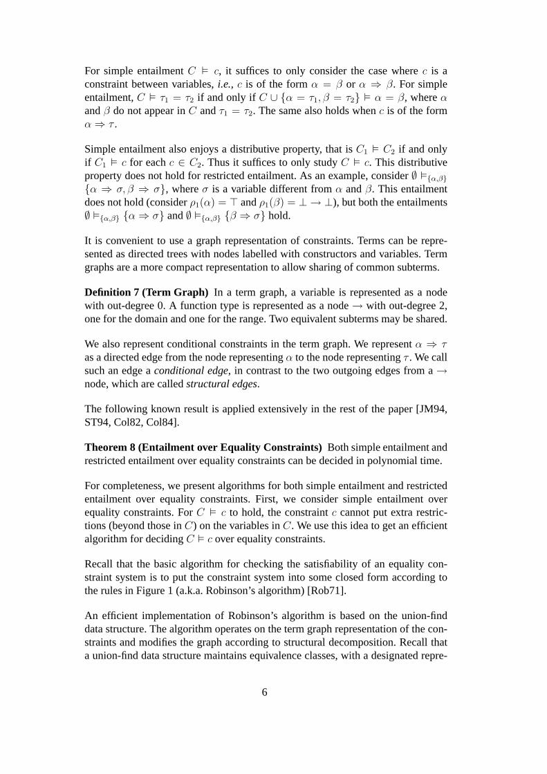
(1) Compute m.g.u. ofC. If fail, output YES; else continue.(2) Compute the congruence closure on the m.g.u. ofC. If α = β is in

the closure, outputYES; else outputNO.

Fig. 3. Simple entailmentC � α = β over equality constraints.

(1) Compute m.g.u. ofC1. If fail, output YES; else continue.(2) Add each term ofC2 to the m.g.u. ofC1 if the term is not already

present.(3) Compute the congruence closure on the term graph obtained in Step 2.(4) Unify the constraints ofC2 in the result obtained in Step 3, and per-

form the following check. For any two non-congruent classes that areunified, we require at least one of the representatives to be a variablein Var(C2) \ E. If this requirement is not met, outputNO; else outputYES.

Fig. 4. Restricted entailmentC1 �E C2 over equality constraints.

next argue its correctness. If the algorithm outputsYES, the constraintα = β iscontained in the congruence closure of the m.g.u. ofC. By Proposition 9, we knowthatC and the congruence closure ofC ’s m.g.u. have the same solutions. ThusC � α = β. On the other hand, if the algorithm outputsNO, the constraintα = β isnot in the congruence closure of the m.g.u. ofC. One can show with an inductionon the structure of theequivalence class representativesof α andβ, i.e., ECR(α)and ECR(β), that any two non-congruent classes admit a valuationρ � C whichmaps the two non-congruent classes to different ground types.

Proposition 9 Let C be an equality constraint system.C andCong(C), the con-gruence closure ofC, have the same set of solutions.

Proof. The rules in Figure 2 preserve solutions. 2

We now consider restricted entailment over equality constraints. The goal is todecideC1 �E C2 for two constraint systemsC1 andC2 andE = Var(C1)∪Var(C2).Recall thatC1 �E C2 if and only if for every valuationρ1 � C1 there exists avaluationρ2 � C2 such thatρ1(α) = ρ2(α) for all α ∈ E. We first study anexample. Consider the two constraint systemsC1 = {α = σ → σ} andC2 = {α =σ1 → σ2} with the interface variableE = {α}. For any valuationρ � C1, we knowρ(α) = τ → τ for someτ . Consider the valuationρ′ of C2 with ρ′(α) = ρ(α)andρ′(σ1) = ρ′(σ2) = ρ(σ). It is easy to see thatρ′ � C2, and thus the relationC1 �E C2 holds. The algorithm for simple entailment given in Figure 3 does notapply since for this example, it would give the answerNO. Notice that ifC1 � C2

(holds iff for all c ∈ C2 we haveC1 � c) thenC1 �E C2 for anyE. The converse,

query. Congruence closure gives a simpler explanation, and also gives an algorithm thatanswers queries in constant time.

8

however, is not true, as shown by the example.

We show how to extend the algorithm for simple entailment to obtain an algorithmfor restricted entailment. The intuition behind the algorithm is that we can relax therequirement of simple entailment to allow internal variables ofC2 to be added toequivalence classes of the term graph representation of the m.g.u. ofC1, as long asno equivalence classes ofC1 are merged. The algorithm is given in Figure 4.2 Thetime complexity of the algorithm isO((m + n) log(m + n)), wherem andn arethe respective sizes ofC1 andC2.

In Figure 4, the choice of representatives for equivalence classes is important. Wepick representatives in the following order, which guarantees that if the representa-tive is in Var(C2) \ E, then there is no variable in Var(C1) or a constructor in theequivalence class:

(1) ⊥,>, and→ nodes;(2) variables in Var(C1);(3) variables in Var(C2) \ E.

We now argue the correctness of the algorithm. Suppose it outputsYES. If C1 is notsatisfiable then clearlyC1 �E C2. Let ρ1 be a satisfying valuation ofC1. Considerthe valuationρ given in Figure 5. First,ρ is clearly well-defined. Letρ2 denote thevaluation obtained by restrictingρ to Var(C2), i.e., the variables inC2. We want toshow thatρ2 � C2. Since the algorithm outputsYES, when adding the constraintsin C2, the only change to the term graph is adding variables in Var(C2) \E to someexisting equivalence classes. By the construction ofρ, one can see thatρ satisfiesall the induced constraints in the term graph at step 4 of the algorithm. Thus, wehaveρ � C1 ∪ C2, and thereforeρ2 � C2. Hence, we haveC1 �E C2. Conversely,suppose the algorithm outputsNO. Then there exist two equivalence classes to beunified neither of whoseECR is a variable in Var(C2) \ E. There are two cases:

• In the first case, oneECR is a variable in Var(C1), sayα. If the other represen-tative is⊥, then any valuationρ1 � C1 with ρ1(α) = > gives a witness forC1 2E C2. The case where the other representative is> or a→ node is similar.If the other representative is a variableβ ∈ Var(C1), any valuationρ1 � C1 withρ1(α) = > andρ1(β) = ⊥ is a witness forC1 2E C2.

• In the second case, bothECRs are constructors. If there is a constructor mismatch,thenC1 ∪ C2 is not satisfiable. SinceC1 is satisfiable, thenC1 2E C2 (Sinceif C1 �E C2, any satisfying valuation forC1 can be extended to a satisfyingvaluation forC2.)

Note that if there is no constructor mismatch (where both representatives are→nodes), the error is detected when trying to unify the terms represented by thesetwo nodes. Thus it falls into one of the above cases.

2 The congruence closure step is again not necessary, but used for a simpler explanation.

9

ρ(α) = ρ1(α) if α ∈ Var(C1)

ρ(α) =

ρ1(ECR(α)) if ECR(α) ∈ Var(C1)

⊥ if ECR(α) ∈ Var(C2) \ E

⊥ if ECR(α) = ⊥

> if ECR(α) = >

ρ(τ1) → ρ(τ2) if ECR(α) = τ1 → τ2

if α ∈ Var(C2) \ E

Fig. 5. Constructed valuationρ.

3 Simple Entailment over Conditional Equality Constraints

In this section, we consider simple entailment over conditional equality constraints.Recall forα⇒ τ to be satisfied by a valuationρ, eitherρ(α) = ⊥ or ρ(α) = ρ(τ).

Consider the constraints{α⇒ >, α⇒ ⊥→ ⊥}. The only solution isα = ⊥. Thefact thatα must be⊥ is not explicit. For entailment, we want to make the fact thatα must be⊥ explicit. Assume that we have run CONDRESOLVE on the constraintsto get a term graphG. For each variableα, we check whether it must be⊥. Ifboth addingα = > to G andα = σ1 → σ2 to G (for fresh variablesσ1 andσ2)fail, α must be⊥, in which case, we addα = ⊥ to G. We repeat this process foreach variable. Notice that this step can be done in polynomial time. We present thismodification to the conditional unification algorithm in Figure 6.

We now present an algorithm for decidingC � α = β andC � α ⇒ β whereCis a system of conditional equality constraints. Notice thatC � α = β holds if andonly if bothC � α ⇒ β andC � β ⇒ α hold. We give the algorithm in Figure 7.The basic idea is to checkC � α ⇒ β holds. We have two cases: (i) whenα is>and (ii) whenα is a function type. In both cases, we requireβ = α. The problemthen reduces to simple entailment over equality constraints. Congruence closureis required to make explicit the implied equalities between terms involving→.Computing strongly connected components is used to make explicit, for example,α = β if both α ⇒ β andβ ⇒ α. It is easy to see that the algorithm runs in worstcase polynomial time in the size ofC.

Theorem 10 The simple entailment algorithm in Figure 7 is correct.

Proof. Suppose that the algorithm outputsYES. Let ρ be a satisfying valuation forC. We have three cases:

• If ρ(α) = ⊥, thenρ � α⇒ β.• If ρ(α) = >, thenρ � C ∪ {α = >}. ThusC ∪ {α = >} is satisfiable. We then

10

Let C be a system of constraints. The following algorithm outputs a termgraph representing the solutions ofC.(1) LetG be the term graph CONDRESOLVE(C).(2) For each variableα in Var(C), check whether it must be⊥: If neither

G∪{α = >} norG∪{α = σ1 → σ2} is satisfiable, addα = ⊥ toG.

Fig. 6. Modified satisfiability algorithm.

haveβ = > is in the closure ofC ∪{α = >}. Hence,ρ � β = >, which impliesthatρ � α⇒ β.

• If ρ(α) = τ1 → τ2 whereτ1 andτ2 are ground types, we haveC∪{α = σ1 → σ2}is satisfiable. We thus haveβ = σ1 → σ2 is in the closure ofC∪{α = σ1 → σ2}.Henceρ � β = σ1 → σ2, and which implies thatρ � α⇒ β.

Combining the three cases, we conclude thatC � α⇒ β.

Suppose the algorithm outputsNO. Then at least one of the two cases returnsFAIL .Assume that the case withα = > returnsFAIL . Thenβ = > is not in the congru-ence closure ofC ∪{α = >}. By assigning all the remainingconditional variablesto ⊥ (variables appearing as the antecedent of the conditional constraints) in thegraph, we can exhibit a witness valuationρ that satisfiesC but does not satisfyα ⇒ β (same as the case for simple entailment over equality constraints). Theother case whereα = σ1 → σ2 is similar. HenceC 2 α⇒ β. 2

4 Restricted Entailment over Conditional Equality Constraints

In this section, we present the main result of this paper, a polynomial time algorithmfor restricted entailment over conditional constraints.

Example 2 (Example Constraints) Consider the constraints:

{α1 ⇒ ⊥, α1 ⇒ σ1, α2 ⇒ σ1, α2 ⇒ σ2, α3 ⇒ σ2, α3 ⇒ >}.

The graph representation of the constraints is given by:

α1

�����

��444

4 α2

��

��444

4 α3

�� ��3

33

⊥ σ1 σ2 >

Notice that the solutions of the constraints in Example 2 with respect to{α1, α2, α3}are all tuples〈v1, v2, v3〉 that satisfy

(v1 = ⊥∧v3 = ⊥)∨ (v1 = ⊥∧v2 = ⊥ ∧v3 = >)∨ (v1 = ⊥∧v2 = > ∧v3 = >)

11

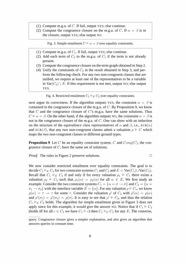
If both of the following cases returnSUCCESS, outputYES; else outputNO.(1) (a) Run the conditional unification algorithm in Figure 6 onC∪{α =

>}. If not satisfiable, thenSUCCESS; else continue.(b) Compute strongly connected components (SCC) on the condi-

tional edges and merge the nodes in every SCC. This step yieldsa modified term graph.

(c) Compute congruence closure on the term graph obtained inStep 1b. We do not consider the conditional edges for comput-ing congruence closure.

(d) If β = > is in the closure,SUCCESS; elseFAIL .(2) (a) Run the conditional unification algorithm in Figure 6 onC∪{α =

σ1 → σ2}, whereσ1 and σ2 are two fresh variables not inVar(C)∪ {α, β}. If not satisfiable, thenSUCCESS; else continue.

(b) Compute strongly connected components (SCC) on the condi-tional edges and merge the nodes in every SCC. This step yieldsa modified term graph.

(c) Compute congruence closure on the term graph obtained inStep 2b. Again, we do not consider the conditional edges for com-puting congruence closure.

(d) If β = σ1 → σ2 is in the closure,SUCCESS; elseFAIL .

Fig. 7. Simple entailmentC � α ⇒ β over conditional equality constraints.

Now suppose we do the following: take pairs of constraints, find their solutions withrespect to{α1, α2, α3}, and take the intersection of the solutions. LetS∗ denotethe set of all valuations. Figure 8 shows the solutions for all the subsets of twoconstraints with respect to{α1, α2, α3}. One can show that the intersection of thesesolutions is the same as the solution for all the constraints. Intuitively, the solutionsof a system of conditional constraints can be characterized by considering all pairsof constraints independently. We can make this intuition formal by putting someadditional requirements on the constraints.

For simplicity, in later discussions, we consider the language without>. With someextra checks, the presented algorithm can be easily adapted to include> in thelanguage.

Here is the route we take to develop a polynomial time algorithm for restrictedentailment over conditional constraints.

Section 4.1We introduce a notion of aclosed systemand show that closed systems havethe property that it is sufficient to consider pairs of conditional constraints indetermining the solutions of the complete system with respect to the interfacevariables.

12

S({α1 ⇒ ⊥, α2 ⇒ σ1}) = {〈v1, v2, v3〉 | v1 = ⊥}S({α2 ⇒ σ1, α2 ⇒ σ2}) = S∗

S({α3 ⇒ σ2, α3 ⇒ >}) = {〈v1, v2, v3〉 | (v3 = ⊥) ∨ (v3 = >)}S({α1 ⇒ ⊥, α2 ⇒ σ1}) = {〈v1, v2, v3〉 | v1 = ⊥}S({α1 ⇒ ⊥, α2 ⇒ σ2}) = {〈v1, v2, v3〉 | v1 = ⊥}S({α1 ⇒ ⊥, α3 ⇒ σ2}) = {〈v1, v2, v3〉 | v1 = ⊥}S({α1 ⇒ ⊥, α3 ⇒ >}) = {〈v1, v2, v3〉 | (v1 = v3 = ⊥) ∨ (v1 = ⊥ ∧ v3 = >)}

S({α1 ⇒ σ1, α2 ⇒ σ1}) = {〈v1, v2, v3〉 | (v1 = ⊥) ∨ (v2 = ⊥) ∨ (v2 = v3)}S({α1 ⇒ σ1, α2 ⇒ σ2}) = S∗

S({α1 ⇒ σ1, α3 ⇒ σ2}) = S∗

S({α1 ⇒ σ1, α3 ⇒ >}) = {〈v1, v2, v3〉 | (v3 = ⊥) ∨ (v3 = >)}S({α2 ⇒ σ1, α3 ⇒ σ2}) = S∗

S({α2 ⇒ σ1, α3 ⇒ >}) = {〈v1, v2, v3〉 | (v3 = ⊥) ∨ (v3 = >)}S({α2 ⇒ σ2, α3 ⇒ σ2}) = {〈v1, v2, v3〉 | (v2 = ⊥) ∨ (v3 = ⊥) ∨ (v2 = v3)}S({α2 ⇒ σ2, α3 ⇒ >}) = {〈v1, v2, v3〉 | (v3 = ⊥) ∨ (v3 = >)}

Fig. 8. Solutions for all subsets of two constraints.

Section 4.2We show that restricted entailment with a pair of conditional constraints can bedecided in polynomial time,i.e., C �E C= ∪ {c1, c2} can be decided in poly-nomial time, whereC= consists of equality constraints, andc1 andc2 are condi-tional constraints.

Section 4.3We show how to reduce restricted entailment to restricted entailment in terms ofclosed systems. In particular, we show how to reduceC1 �E C2 to C ′

1 �E′ C ′2

whereC ′2 is closed.

Combining the results, we arrive at a polynomial time algorithm for restricted en-tailment over conditional constraints.

4.1 Closed Systems

We define the notion of a closed system and show the essential properties of closedsystems for entailment. Before presenting the definitions, we first demonstrate theidea with the example in Figure 9a. LetC denote the constraints in this example,with α andβ the interface variables, andσ, σ1, andσ2 the internal variables. Theintersection of the solutions of all the pairs of constraints is:α is either⊥ or τ → ⊥,andβ is either⊥ or τ ′ → ⊥ for someτ andτ ′. However, the solutions ofC requirethat if α = τ → ⊥ andβ = τ ′ → ⊥, and bothτ andτ ′ are non-⊥, thenτ = τ ′,

13

�

β��→

��� 66

6 →��

� 666

σ1

''OOOOOOO ⊥ σ2

�����

⊥σ

α��vvnnnnnnnn β

�� ''PPPPPPP

→��

� 666 →

��� 55

5 →��

� 555 →

��� 66

6

α1

++WWWWWWWWWWWWWWWW σ3 σ1

''OOOOOOO ⊥ σ2

�����

⊥ β1

kk

σ4

σ

(a) Example system. (b) Example system closed.

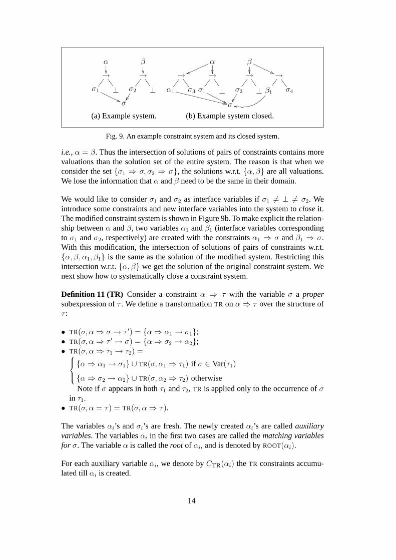
Fig. 9. An example constraint system and its closed system.

i.e., α = β. Thus the intersection of solutions of pairs of constraints contains morevaluations than the solution set of the entire system. The reason is that when weconsider the set{σ1 ⇒ σ, σ2 ⇒ σ}, the solutions w.r.t.{α, β} are all valuations.We lose the information thatα andβ need to be the same in their domain.

We would like to considerσ1 andσ2 as interface variables ifσ1 6= ⊥ 6= σ2. Weintroduce some constraints and new interface variables into the system tocloseit.The modified constraint system is shown in Figure 9b. To make explicit the relation-ship betweenα andβ, two variablesα1 andβ1 (interface variables correspondingto σ1 andσ2, respectively) are created with the constraintsα1 ⇒ σ andβ1 ⇒ σ.With this modification, the intersection of solutions of pairs of constraints w.r.t.{α, β, α1, β1} is the same as the solution of the modified system. Restricting thisintersection w.r.t.{α, β} we get the solution of the original constraint system. Wenext show how to systematically close a constraint system.

Definition 11 (TR) Consider a constraintα ⇒ τ with the variableσ a propersubexpression ofτ . We define a transformationTR onα ⇒ τ over the structure ofτ :

• TR(σ, α⇒ σ → τ ′) = {α⇒ α1 → σ1};• TR(σ, α⇒ τ ′ → σ) = {α⇒ σ2 → α2};• TR(σ, α⇒ τ1 → τ2) = {α⇒ α1 → σ1} ∪ TR(σ, α1 ⇒ τ1) if σ ∈ Var(τ1)

{α⇒ σ2 → α2} ∪ TR(σ, α2 ⇒ τ2) otherwiseNote if σ appears in bothτ1 andτ2, TR is applied only to the occurrence ofσ

in τ1.• TR(σ, α = τ) = TR(σ, α⇒ τ).

The variablesαi’s andσi’s are fresh. The newly createdαi’s are calledauxiliaryvariables. The variablesαi in the first two cases are called thematching variablesfor σ. The variableα is called theroot of αi, and is denoted byROOT(αi).

For each auxiliary variableαi, we denote byCTR(αi) the TR constraints accumu-lated till αi is created.

14

Putting this definition to use on the constraint system in Figure 9a,TR(σ1, α ⇒σ1 → ⊥) yields the constraintα⇒ α1 → σ3 (shown in Figure 9b).

To understand the definition ofCTR(αi), considerTR(σ, α⇒ ((σ → ⊥) → ⊥)) ={α⇒ α1 → σ1, α1 ⇒ α2 → σ2}, whereα1 andα2 are the auxiliary variables. WehaveCTR(α1) = {α ⇒ α1 → σ1} andCTR(α2) = {α ⇒ α1 → σ1, α1 ⇒ α2 →σ2}.

Definition 12 (Closed Systems)A system of conditional constraintsC ′ is closedw.r.t. a set of variablesE in C after the following steps:

(1) LetC ′ = CONDRESOLVE(C).(2) SetW toE.(3) For each variableα ∈ W , if α⇒ τ is inC ′, whereσ ∈ Var(τ), andσ ⇒ τ ′ ∈

C ′, addTR(σ, α ⇒ τ) to C ′. Let α′ be the matching variable forσ and addα′ ⇒ τ ′ toC ′.

(4) SetW to the set of auxiliary variables created in Step 3 and repeat Step 3 untilW is empty.

Step 3 of this definition warrants explanation. In the exampleTR(σ1, α ⇒ σ1) weadd the constraintα⇒ α1 → σ3 with α1 as the matching variable forσ1. We wantto ensure thatα1 andσ1 are actually the same, so we add the constraintα1 ⇒ σ.This process must be repeated to expose all such internal variables (such asσ1 andσ2).

Next we give the definition of aforced variable. Given a valuationρ for the interfacevariables, if an internal variableσ is determined already byρ, thenσ is forced byρ.For example, in Figure 9a, ifα is non-⊥, then the value ofσ1 is forced byα.

Definition 13 (Forced Variables) We say that an internal variableσ is forcedby avaluationρ if any one of the following holds (A is the set of auxiliary variables)

• ECR(σ) = ⊥;• ECR(σ) = α, whereα ∈ E ∪ A;• ECR(σ) = τ1 → τ2;• ρ(α) 6= ⊥ andα⇒ τ is a constraint whereσ ∈ Var(τ) andα ∈ E ∪ A;• σ′ is forced byρ to a non-⊥ value andσ′ ⇒ τ is a constraint whereσ ∈ Var(τ).

Theorem 14 Let C be a closed system of constraints w.r.t. a set of interface vari-ablesE, and letA be the set of auxiliary variables ofC. Let C= andC⇒ be thesystems of equality constraints and conditional constraints respectively. Then

S(C) |E∪A =⋂

ci,cj∈C⇒

S(C= ∪ {ci, cj}) |E∪A .

In other words, it suffices to consider pairs of conditional constraints in determiningthe solutions of a closed constraint system.

15

Proof. SinceC contains all the constraints inC= ∪ {ci, cj} for all i andj, thus itfollows that

S(C) |E∪A ⊆⋂

ci,cj∈C⇒

S(C= ∪ {ci, cj}) |E∪A .

It remains to show

S(C) |E∪A ⊇⋂

ci,cj∈C⇒

S(C= ∪ {ci, cj}) |E∪A .

Let ρ be a valuation in⋂

ci,cj∈C⇒ S(C= ∪ {ci, cj}) |E∪A. It suffices to show thatρcan be extended to a satisfying valuationρ′ for C. To show this, it suffices to findan extensionρ′ of ρ for C such thatρ′ � C= ∪ {ci, cj} for all i andj.

Consider the valuationρ′ obtained fromρ by mapping all the internal variables notforced byρ (in C) to⊥. The valuationρ′ can be uniquely extended to satisfyC iffor anyci andcj, c′i andc′j, if σ is forced byρ in bothC=∪{ci, cj} andC=∪{c′i, c′j},then it is forced to the same value in both systems. The value thatσ is forced to byρ is denoted byρ!(σ).

We prove by cases (cf. Definition 13) that ifσ is forced byρ, it is forced to thesame value in pairs of constraints. LetCi,j denoteC= ∪ {ci, cj} andCi′,j′ denoteC= ∪ {c′i, c′j}.

• If ECR(σ) = ⊥, thenσ is forced to the same value, i.e.,⊥, becauseσ = ⊥ ∈ C=.• If ECR(σ) = α, with α ∈ E ∪ A, thenσ is forced toρ(α) in both systems,

becauseσ = α ∈ C=.• If ECR(σ) = τ1 → τ2, one can show thatρ forcesσ to the same value with an

induction over the structure ofECR(σ) (with the two cases above as base cases).• Assumeσ is forced inCi,j becauseα ⇒ τ1 ∈ Ci,j with ρ(α) 6= ⊥ and forced inCi′,j′ becauseβ ⇒ τ2 ∈ Ci′,j′ with ρ(β) 6= ⊥. For each extensionρ1 of ρ withρ1 � Ci,j, and for each extensionρ2 of ρ with ρ2 � Ci′,j′, we have

ρ(α) = ρ1(α) = ρ1(τ1)

ρ(β) = ρ2(β) = ρ2(τ2)

Consider the constraint systemC= ∪ {α⇒ τ1, β ⇒ τ2}. The valuationρ can beextended toρ3 with ρ3 � C= ∪ {α⇒ τ1, β ⇒ τ2}. Thus we have

ρ(α) = ρ3(α) = ρ3(τ1)

ρ(β) = ρ3(β) = ρ3(τ2)

Therefore,ρ1(τ1) = ρ3(τ1) andρ2(τ2) = ρ3(τ2). Hence,ρ1(σ) = ρ3(σ) andρ2(σ) = ρ3(σ), which implyρ1(σ) = ρ2(σ). Thusσ is forced to the same value.

16

• Assumeσ is forced inCi,j becauseσ1 is forced to a non-⊥ value andσ1 ⇒ τ1 ∈Ci,j and is forced inCi′,j′ becauseσ2 is forced to a non-⊥ value andσ2 ⇒ τ2 ∈Ci′,j′. BecauseC is a closed system, we must have two interface variables orauxiliary variablesα andβ with bothα⇒ τ1 andβ ⇒ τ2 appearing inC. Sinceσ1 andσ2 are forced, then we must haveρ(α) = ρ!(σ1) andρ(β) = ρ!(σ2), thusσ must be forced to the same value by the previous case.

• Assumeσ is forced inCi,j becauseρ(α) 6= ⊥ andα ⇒ τ1 ∈ Ci,j and forced inCi′,j′ becauseσ2 is forced to a non-⊥ value andσ2 ⇒ τ2 ∈ Ci′,j′. This case issimilar to the previous case.

• The remaining case, whereσ is forced inCi,j becauseσ1 is forced to a non-⊥ value andσ1 ⇒ τ1 ∈ Ci,j and is forced inCi′,j′ becauseρ(α) 6= ⊥ andα⇒ τ2 ∈ Ci′,j′, is symmetric to the above case.

2

4.2 Entailment of Pair Constraints

In the previous subsection, we saw that a closed system can be decomposed intopairs of conditional constraints. In this section, we show how to efficiently deter-mine entailment if the right-hand side consists of a pair of conditional constraints.

We first state a lemma (Lemma 15) which is important in finding a polynomialalgorithm for entailment of pair constraints.

Lemma 15 Let C1 be a system of conditional constraints andC2 be a system ofequalityconstraints withE = Var(C1)∩Var(C2). The decision problemC1 �E C2

is solvable in polynomial time.

Proof. Consider the following algorithm. We first solveC1 using CONDRESOLVE,and add the terms appearing inC2 to the resulting term graph forC1. Then forany two terms appearing in the term graph, we decide, using the simple entailmentalgorithm in Figure 7, whether the two terms are the same. For terms which areequivalent we merge their equivalence classes. Next, for each of the constraints inC2, we merge the left and right sides. For any two non-congruent classes that areunified, we require at least one of the representatives be a variable in Var(C2)\E. Ifthis requirement is not met, the entailment does not hold. Otherwise, the entailmentholds.

If the requirement is met, then it is routine to verify that the entailment holds. Sup-pose the requirement is not met,i.e., there exist two non-congruent classes whichare unified and none of whoseECRs is a variables in Var(C2) \ E. Since the twoclasses are non-congruent, we can choose a satisfying valuation forC1 which mapsthe two classes to different values (This is possible because, otherwise, we would

17

have proven that they are the same with the simple entailment algorithm for condi-tional constraints.) The valuationρ |E cannot be extended to a satisfying valuationfor C2 because, otherwise, this contradicts the fact thatC1 ∪ C2 entails the equiva-lence of the two non-congruent terms. 2

Theorem 16 Let C1 be a system of conditional constraints. LetC= be a systemof equality constraints. The following three decision problems can be solved inpolynomial time:

(1) C1 �E C= ∪ {α⇒ τ1, β ⇒ τ2}, whereα, β ∈ E.(2) C1 �E C= ∪ {α⇒ τ1, µ⇒ τ2}, whereα ∈ E andµ /∈ E.(3) C1 �E C= ∪ {µ1 ⇒ τ1, µ2 ⇒ τ2}, whereµ1, µ2 /∈ E.

Proof.

(1) For the caseC1 �E C= ∪ {α ⇒ τ1, β ⇒ τ2}, notice thatC1 �E C= ∪ {α ⇒τ1, β ⇒ τ2} iff the following entailments hold• C1 ∪ {α = ⊥, β = ⊥} �E C=

• C1 ∪ {α = ⊥, β = ν1 → ν2} �E C= ∪ {β = τ2}• C1 ∪ {α = σ1 → σ2, β = ⊥} �E C= ∪ {α = τ1}• C1 ∪ {α = σ1 → σ2, β = ν1 → ν2} �E C= ∪ {α = τ1, β = τ2}whereσ1, σ2, ν1, andν2 are fresh variables not in Var(C1) ∪ Var(C2).

Notice that each of the above entailments reduces to entailment of equalityconstraints, which can be decided in polynomial time by Lemma 15.

(2) For the caseC1 �E C= ∪ {α⇒ τ1, µ⇒ τ2}, we consider two cases:• C1 ∪ {α = ⊥} �E C= ∪ {µ⇒ τ2};• C1 ∪ {α = σ1 → σ2} �E C= ∪ {α = τ1, µ⇒ τ2}whereσ1 andσ2 are fresh variables not in Var(C1) ∪ Var(C2).

We have a few cases.• ECR(µ) = ⊥• ECR(µ) = τ1 → τ2• ECR(µ) ∈ E• ECR(µ) /∈ ENotice that the only interesting case is the last case (ECR(µ) /∈ E) when thereis a constraintβ = τ in C= andµ appears inτ . For this case, we consider alltheO(n) resulted entailments by settingβ to some appropriate value accord-ing to the structure ofτ , i.e., we consider all the possible values forβ. Forexample, ifτ = (µ→ ⊥) → µ, we consider the following cases:• β = ⊥;• β = ⊥ → ν1;• β = (⊥ → ν2) → ν1;• β = ((ν3 → ν4) → ν2) → ν1

whereν1,ν2,ν3, andν4 are fresh variables.Each of the entailments will have only equality constraints on the right-

hand side. Thus, these can all be decided in polynomial time. Together, the

18

�

β��→

666 →

�������� 66

6

⊥ ⊥σ0

�yyrrr

rrr� ''PPPPPPP

→��

� 666 →

555 →

�������� 55

5 →��� 66

6

α1 σ3 ⊥ ⊥ β1 σ4

σ0

(a)C1. (b)C1 closed.

�

β��→

��� 66

6 →��

� 666

σ1

''OOOOOOO ⊥ σ2

�����

⊥σ

α��vvnnnnnnnn β

�� ''PPPPPPP

→��

� 666 →

��� 55

5 →��

� 555 →

��� 66

6

α1

++WWWWWWWWWWWWWWWW σ3 σ1

''OOOOOOO ⊥ σ2

�����

⊥ β1

kk

σ4

σ

(c)C2. (d)C2 closed.

Fig. 10. Example entailment.

entailment can be decided in polynomial time.(3) For the caseC1 �E C= ∪ {µ1 ⇒ τ1, µ2 ⇒ τ2}, the same idea as in the

second case applies as well. The sub-case which is slightly different is when,for example,µ2 appears inτ1 only. In this case, for someβ andτ , β = τ isin C= whereµ1 occurs inτ . Let τ ′ = τ [τ1/µ1], whereτ [τ1/µ1] denotes thetype obtained fromτ by replacing each occurrence ofµ1 by τ1. Again, weconsiderO(n) entailments with right-side an equality constraint system byassigningβ appropriate values according to the structure ofτ ′. Thus this formof entailment can also be decided in polynomial time.

2

4.3 Reduction of Entailment to Closed Systems

We now reduce an entailmentC1 �E C2 to entailment of closed systems, thus com-pleting the construction of a polynomial time algorithm for restricted entailmentover conditional constraints.

Unfortunately we cannot directly use the closed systems forC1 andC2 as demon-strated by the example in Figure 10. Figures 10a and 10c show two constraint sys-temsC1 andC2. Suppose we want to decideC1 �{α,β} C2. One can verify that theentailment does hold. Figures 10b and 10d show the closed systems forC1 andC2,which we nameC ′

1 andC ′2. Note that we include theTR constraints ofC2 inC ′

1. Onecan verify that the entailmentC ′

1 �{α,β,α1,β1} C′2 does not hold (takeα = β = ⊥,

19

α1 = ⊥ → ⊥, andβ1 = ⊥ → >, for example). The reason is that there is someinformation aboutα1 andβ1 missing fromC ′

1. In particular, when bothα1 andβ1

are forced, we should haveα1 ⇒ σ′ andβ1 ⇒ σ′ (actually in this case they satisfythe stronger relation thatα1 = β1). By replacingα⇒ α1 → σ3 andβ ⇒ β1 → σ4

with α = α1 → σ3 andβ = β1 → σ4 (because that is when both are forced),we can decide thatα1 = β1. The following definition of acompletiondoes exactlywhat we have described.

Definition 17 (Completion) Let C be a closed constraint system ofC0 w.r.t. E.Let A be the set of auxiliary variables. For each pair of variablesαi andβj in A,let C(αi, βj) = CTR(αi) ∪ CTR(βj) (see Definition 11) andC=(αi, βj) be theequality constraints obtained by replacing⇒ with = in C(αi, βj). Decide whetherC ∪ C=(αi, βj) �{αi,βj} {αi ⇒ σ, βj ⇒ σ} (cf. Theorem 16). If the entailmentholds, add the constraintsαi ⇒ σ(αi,βj) andβj ⇒ σ(αi,βj) to C, whereσ(αi,βj) isa fresh variable unique forαi andβj. The resulting constraint system is called thecompletionof C.

Theorem 18 Let C1 andC2 be two conditional constraint systems. LetC ′2 be the

closed system ofC2 w.r.t. toE = Var(C1) ∩ Var(C2) with A the set of auxiliaryvariables. Construct the closed system forC1 w.r.t. E with A′ the auxiliary vari-ables, and add theTR constraints of closingC2 to C1 after closingC1. Let C ′

1 bethe completion of modifiedC1. We haveC1 �E C2 iff C ′

1 �E∪A∪A′ C′2.

Proof. (⇐): AssumeC ′1 �E∪A∪A′ C

′2. Let ρ � C1. We can extendρ to ρ′ which

satisfiesC ′1. SinceC ′

1 �E∪A∪A′ C′2, then there existsρ′′ such thatρ′′ � C ′

2 withρ′ |E∪A∪A′= ρ′′ |E∪A∪A′. Sinceρ′′ � C ′

2, we haveρ′′ � C2. Also ρ |E= ρ′ |E=ρ′′ |E. Therefore,C1 �E C2.

(⇒): AssumeC1 �E C2. Let ρ � C ′1. Thenρ � C1. Thus there existsρ′ � C2

with ρ |E= ρ′ |E. We extendρ′ |E to ρ′′ with ρ′′(α) = ρ′(α) if α ∈ E andρ′′(α) = ρ(α) if α ∈ (A ∪ A′). It suffices to show thatρ′′ can be extended withmappings for variables in Var(C ′

2) \ (E ∪ A ∪ A′) = Var(C ′2) \ (E ∪ A), because

ρ′′ |E∪A∪A′= ρ |E∪A∪A′.

Notice that all theTR constraints inC ′2 are satisfied by some extension ofρ′′, be-

cause they also appear inC ′1. Also the constraintsC2 are satisfied by some ex-

tension ofρ′′. It remains to show that the internal variables ofC ′2 are forced by

ρ′′ to the same value if they are forced byρ′′ in either theTR constraints orC2.Suppose there is an internal variableσ forced to different values byρ′′. W.L.O.G.,assume thatσ is forced byρ′′ becauseρ′′(αi) 6= ⊥ andαi ⇒ σ and forced becauseρ′′(βj) 6= ⊥ andβj ⇒ σ for some interface or auxiliary variablesαi andβj. Con-sider the interface variablesROOT(αi) andROOT(βj) (see Definition 11). Since thecompletion ofC1 does not include constraints{αi ⇒ σ′, βj ⇒ σ′}, thus we canassignROOT(αi) andROOT(βj) appropriate values to forceαi andβj to differentnon-⊥ values. However,C2 requiresαi andβj to have the same non-⊥ value. Thus,

20

if there is an internal variableσ forced to different values byρ′′, we can constructa valuation which satisfiesC1, but the valuation restricted toE cannot be extendedto a satisfying valuation forC2. This contradicts the assumption thatC1 �E C2.To finish the construction of a desired extension ofρ′′ that satisfiesC ′

2, we set thevariables which are not forced to⊥.

One can easily verify that this valuation must satisfyC ′2. HenceC ′

1 �E∪A∪A′ C′2. 2

4.4 Putting Everything Together

Theorem 19 (Main) Restricted entailment for conditional constraints can be de-cided in polynomial time.

Proof. Consider the problemC1 �E C2. By Theorem 18, it is equivalent to testingC ′

1 �E∪A∪A′ C′2 (see Theorem 18 for the appropriate definitions ofC ′

1, C′2, A, and

A′). Notice thatC ′1 andC ′

2 are constructed in polynomial time in sizes ofC1 andC2.Now by Theorem 14, this is equivalent to checkingO(n2) entailment problems ofthe formC ′

1 �E∪A∪A′ C2′= ∪ {ci, cj}, whereC2′= denote the equality constraints ofC ′

2 andci andcj are two conditional constraints ofC ′2. And by Theorem 16, we can

decide each of these entailments in polynomial time. Putting everything together,we have a polynomial time algorithm for restricted entailment over conditionalconstraints. 2

Because unification is polynomial-time complete (PTIME-complete), it immedi-ately follows that restricted entailment for conditional equality constraints is alsocomplete for polynomial time.

Corollary 20 (PTIME-completeness) Restricted entailment for conditional equal-ity constraints is PTIME-complete.

5 Extended Conditional Constraints

In this section, we show that restricted entailment for a natural extension of thestandard conditional constraint language is coNP-complete. This section is helpfulfor a comparison between this constraint language with the standard conditionalconstraint language, which we consider in Sections 3 and 4. The results in thissection provide one natural boundary between tractable and intractable entailmentproblems.

We extend the constraint language with a new constructα ⇒ (τ1 = τ2), whichholds iff eitherα = ⊥ or τ1 = τ2. We call this form of constraintsextended condi-

21

tional equality constraints. To see that this construct indeed extendsα⇒ τ , noticethatα⇒ τ can be encoded in the new constraint language asα⇒ (α = τ).

This extension is interesting because many equality based program analyses can benaturally expressed with this form of constraints. An example analysis that uses thisform of constraints is the equality based flow analysis for higher order functionallanguages [Pal98].

Note that satisfiability for this extension can still be decided in almost linear timewith basically the same algorithm outlined for conditional equality constraints. Weconsider restricted entailment for this extended language.

In the rest of this section, we consider the restricted entailment problem for ex-tended conditional constraints. We show that the decision problemC1 �E C2 forextended conditional constraints is coNP-complete.

We define the decision problem NENT as the problem of deciding whetherC1 2E

C2, whereC1 andC2 are systems of extended conditional equality constraints andE = Var(C1) ∩ Var(C2).

Theorem 21 The decision problem NENT for extended conditional constraints isin NP.

Proof. LetC1 andC2 be two extended constraint systems, and letE = Var(C1) ∩Var(C2). For each variableα in Var(C1), we guess whetherα is⊥,>, orα1 → α2

for some fresh variablesα1 andα2. We add these constraints toC1 to obtainC ′1.

For eachα in E, we add toC2 the constraintsα = ⊥, α = >, or α = α1 → α2

depending on what we guessed forC1. Notice now thatC ′1 is a system of equality

constraints.C ′2, however, may still have some conditional constraints. This means

that our guess for the variablesE needs to be refined to get rid of these conditionalconstraints inC ′

2. In C ′2, for each conditional constraint with a fresh variableαi

(the generated variables) as antecedent, we guess the value ofαi and add the corre-sponding constraints to bothC ′

1 andC ′2. This process is repeated until there are no

more conditional constraints inC ′2 with any fresh variables as antecedents. Since

there are at mostO(|C2|) number of conditional constraints inC2, thus we make atmostO(|C2|) number of guesses. Finally, conditional constraints with variables inVar(C2) \ E as antecedents are discarded since these constraints do not affect thesolutions of the constraints w.r.t.E.

Let C ′′1 andC ′′

2 be the resulting constraint systems. Notice they are equality con-straints. Thus at the end, we turn the problem into entailment over equality con-straints, which we can decide in polynomial time. The guessing step takes timepolynomial in|C1| and|C2|. Thus NENT is in NP. 2

Next we show that the problem NENT is hard for NP, and thus an efficient algo-

22

α

��

yyyyy FFF

FF

τ1 τ2

αxi

��

αxi

��

vvvvvv JJJ

JJJ

tttttt HHH

HHH

⊥ τxi >(a) (b)

αc1i

��

αc2i

��

αc3i

��

���� ;;

;;���� ;;

;;���� 77

77

⊥ µci1 µci

2 >

αx2

��

αx4

��

αx7

��

���� <<

<<��

�� <<<<

���� 88

88

⊥ µci1 µci

2 >

(c) (d)

Fig. 11. Graph representations of constraints.

rithm is unlikely to exist for the problem. The reduction actually shows that withextended conditional constraints, evenatomicrestricted entailment (only variables,⊥, and> are in the constraint system) is coNP-hard.

Theorem 22 The decision problem NENT is NP-hard.

Proof. We reduce 3-CNFSAT to NENT. As mentioned, the reduction shows thateven atomic restricted entailment over extended conditional constraints is coNP-complete.

Letψ be a boolean formula in 3-CNF form and let{x1, x2, . . . , xn} and{c1, c2, . . . , cm}be the boolean variables and clauses inψ respectively. For each boolean variablexi in ψ, we create two term variablesαxi

andαxi, which we use to decide the truth

value ofxi. The value⊥ is treated as the boolean value false and any non-⊥ valueis treated as the boolean value true.

Note, in a graph, a constraint of the formα⇒ (τ1 = τ2) is represented as shown inFigure 11a.

First we need to ensure that a boolean variable takes on at most one truth value.We associate with eachxi constraintsCxi

, graphically represented as shown inFigure 11b, whereτxi

is some internal variable. These constraints guarantee that atleast one ofαxi

andαxiis ⊥. These constraints still allow bothαxi

andαxito be

⊥, which we deal with below.

In the following, letαx = αx. For each clauseci = c1i ∨ c2i ∨ c3i of ψ, we createconstraintsCci

that ensure every clause is satisfied by a truth assignment. A clauseis satisfied if at least one of the literals is true, which is the same as saying thatthe negations of the literals cannot all be true simultaneously. The constraints arein Figure 11c, whereµci

1 andµci2 are internal variables associated withci. As an

23

αx1

��

αx1

��

αx2

��

αx2

��

· · · αxn

��

αxn

��

|||| ===

=���

� BBBB

|||| ===

=���

� BBBB · · ·

wwww CC

CC���

� DDDD

αx1 ν1

��

αx1 αx2 ν2

��

αx2 · · · αxn νn

��

αxn

oooooooOOOOOOO

iiiiiiiiiiiUUUUUUUUUU · · ·

}}zzz ((RRRRR

{{{{

PPPPPPPP

⊥ µ1 · · · µn−1 >

Fig. 12. Constructed constraint systemC2.

example considerci = x2 ∨ x4 ∨ x7. The constraintsCciare shown in Figure 11d.

We let C1 be the union of all the constraintsCxiandCcj

for 1 ≤ i ≤ n and1 ≤ j ≤ m, i.e.,

C1 = (n⋃

i=1

Cxi) ∪ (

m⋃j=1

Ccj)

There is one additional requirement that we want to enforce: not bothαxiandαxi

are⊥. This cannot be enforced directly inC1. We construct constraints forC2 toenforce this requirement. The idea is that if for anyxi, the term variablesαxi

andαxi

are both⊥, then the entailment holds.

We now proceed to constructC2. The constraintsC2 represented graphically areshown in Figure 12. In the constraints, all the variables exceptαxi

andαxiare

internal variables. These constraints can be used to enforce the requirement that forall xi at least one ofαxi

andαxiis non-⊥. The intuition is that ifαxi

andαxiare

both⊥, the internal variableνi can be⊥, which breaks the chain of conditionaldependencies along the bottom of Figure 12, allowingµ1, . . . , µi−1 to be set to⊥andµi, . . . , µn−1 to be set to>.

We let the set of interface variablesE = {αxi, αxi

| 1 ≤ i ≤ n}. One can showthatψ is satisfiable iffC1 2E C2. To prove the NP-hardness result, observe thatthe described reduction is a polynomial-time reduction. Thus, the decision problemNENT is NP-hard.

We let the set of interface variablesE = {αxi, αxi

| 1 ≤ i ≤ n}. We show thatψ issatisfiable iffC1 2E C2. Assume thatψ is satisfiable. Letf : {xi | 1 ≤ i ≤ n} →{0, 1} be a satisfying assignment forψ. We construct fromf a valuationρ for thevariablesE such thatρ can be extended to a satisfying valuation forC1 while itcannot be extended to a satisfying valuation forC2. The existence of such aρ issufficient to conclude thatC1 2E C2. We constructρ as follows ρ(αxi

) = ⊥ ∧ ρ(αxi) = > if f(xi) = 0

ρ(αxi) = > ∧ ρ(αxi

) = ⊥ if f(xi) = 1

24

The valuationρ can be extended to a satisfying valuationρ1 for C1. For eachboolean variablexi, there is a unique way to extendρ to satisfy the constraintsin Cxi

, namelyρ1(τxi) = ⊥ if ρ(αxi

) = > andρ1(τxi) = > otherwise. For each

clauseci = c1i ∨c2i ∨c3i , at least one off(c1i ), f(c2i ), andf(c3i ) is 1. Thus, at least oneof ρ(α

c1i), ρ(α

c2i), andρ(α

c3i) is⊥. Assumeρ(α

cji

) is⊥ for somej with 1 ≤ j ≤ 3.

We mapρ′(µcik ) = ⊥ for all 1 ≤ k < j andρ′(µci

k ) = > for all j ≤ k < 3. Theextension clearly satisfies the constraintsCci

for all ci. Thusρ can be extended to asatisfying valuation forC1.

As for C2, ρ cannot be extended to a satisfying assignment. Notice that it requiresνi to be mapped to> for all i. This would result in requiring mappingµ1 to⊥ andµn−1 to> and mappingµi = µj for all 1 ≤ i, j ≤ n−1, which is impossible. Thusall extensions ofρ do not satisfyC2. And therefore, we haveC1 2E C2.

For the other direction, assume thatC1 2E C2. Then there exists aρ1 � C1 and theredoes not exist aρ2 � C2 with ρ1(α) = ρ2(α) for all α ∈ E. SinceC1 is satisfiable,this is equivalent to saying that there exists aρ on the variablesE such thatρ canbe extended to a satisfying valuation forC1 and no extensions ofρ satisfiesC2.

We construct fromρ a satisfying assignment for the boolean formulaψ. First noticethat for each boolean variablexi, ρ must map exactly one of the two type variablesαxi

andαxito ⊥ and exact one to a non-⊥ value. To see this noticeρ(αxi

) andρ(αxi

) cannot both be non-⊥, or the constraintsCxiwould then require⊥ and> to

be unified. Ifρ(αxi) andρ(αxi

) are both⊥, thenρ can be extended to a satisfyingvaluation forC2. In particular,ρ′(νi) = ⊥ if both ρ(αxi

) andρ(αxi) are⊥. For the

µj ’s, we letρ′(µj) = ⊥ if j < i andρ(µj) = > if j ≥ i. It is easy to see thatρ′ � C2. Thus we have shown for each variablexi exactly one ofρ(αxi

) andρ(αxi)

is⊥ and exactly one is a non-⊥ value.

Now we can show how to construct fromρ a satisfying assignmentf of ψ. We let f(xi) = 0 ∧ f(xi) = 1 if ρ(αxi) = ⊥

f(xi) = 1 ∧ f(xi) = 0 otherwise

We show thatf satisfies each clause ofψ. Let ci = c1i ∨ c2i ∨ c3i be a clause ofψ. Consider the constraintsCci

. At least one ofρ(αc1i

), ρ(αc2i

), andρ(αc3i

) must

be⊥. W.L.O.G., assume thatρ(αc1i

) is ⊥. Thenρ(αc1i) is non-⊥. Thus,f(c1i ) is

1. Therefore,f satisfies the clauseci. Hence,f satisfies every clause ofψ, andfsatisfiesψ itself. 2

We thus have shown that the entailment problem over extended conditional con-straints is coNP-complete. The result holds even if all the constraints are restrictedto be atomic.

25

Theorem 23 The decision problemC1 �E C2 over extended conditional con-straints is coNP-complete.

6 Conclusions and Future Work

We have given a complete characterization of the complexities of deciding entail-ment for conditional equality constraints over finite types (finite trees). There are afew related problems to be considered:

• What happens if we allow recursive types (i.e., regular trees)?• What is the relationship with strict constructors (i.e., if c(⊥) = ⊥)?• What is the relationship with a type system equivalent to the equality-based flow

systems [Pal98]? In this type system, the only subtype relation is given by⊥ ≤t1 → t2 ≤ >, and there is no non-trivial subtyping between function types.

We believe the same or similar techniques can be used to address the above men-tioned problems, and many of the results should carry over to these problem do-mains.

Acknowledgments

This research was supported in part by the National Science Foundation grant No.CCR-0085949 and NASA Contract No. NAG2-1210. Jeff Foster, Anders Møller,and the anonymous referees of ESOP’01 provided useful feedbacks on an earlierversion of this paper.

References

[And94] L.O. Andersen.Program Analysis and Specialization for the C Pro-gramming Language. PhD thesis, DIKU, University of Copenhagen,May 1994. DIKU report 94/19.

[AWL94] A. Aiken, E. Wimmers, and T.K. Lakshman. Soft typing with con-ditional types. InProceedings of the 21th Annual ACM SIGPLAN-SIGACT Symposium on Principles of Programming Languages, pages163–173, January 1994.

[Col82] A. Colmerauer. Prolog and infinite trees. In K. L. Clark and S.-A. Tarnlund, editors,Logic Programming, pages 231–251. AcademicPress, London, 1982.

26

[Col84] A. Colmerauer. Equations and inequations on finite and infinite trees. In2nd International Conference on Fifth Generation Computer Systems,pages 85–99, 1984.

[FA96] M. Fahndrich and A. Aiken. Making set-constraint based program anal-yses scale. InFirst Workshop on Set Constraints at CP’96, Cambridge,MA, August 1996. Available as Technical Report CSD-TR-96-917,University of California at Berkeley.

[FF97] C. Flanagan and M. Felleisen. Componential set-based analysis. InProceedings of the 1997 ACM SIGPLAN Conference on ProgrammingLanguage Design and Implementation, June 1997.

[FFA00] J. Foster, M. Fahndrich, and A. Aiken. Monomorphic versus polymor-phic flow-insensitive points-to analysis for c. InProceedings of the 7thInternational Static Analysis Symposium, pages 175–198, 2000.

[FFK+96] C. Flanagan, M. Flatt, S. Krishnamurthi, S. Weirich, and M. Felleisen.Catching bugs in the web of program invariants. InProceedings of the1996 ACM SIGPLAN Conference on Programming Language Designand Implementation, pages 23–32, May 1996.

[FFSA98] M. Fahndrich, J. Foster, Z. Su, and A. Aiken. Partial online cycle elim-ination in inclusion constraint graphs. InProceedings of the 1998 ACMSIGPLAN Conference on Programming Language Design and Imple-mentation, pages 85–96, Montreal, CA, June 1998.

[GJS96] J. Gosling, B. Joy, and G. Steele.The Java Language Specification.Addison Wesley, 1996.

[Hei94] N. Heintze. Set based analysis of ML programs. InProceedings of the1994 ACM Conference on LISP and Functional Programming, pages306–17, June 1994.

[Hen92] F. Henglein. Global tagging optimization by type inference. In1992ACM Conference on Lisp and Functional Programming, pages 205–215, June 1992.

[HR97] F. Henglein and J. Rehof. The complexity of subtype entailment forsimple types. InProceedings of the 12th Annual IEEE Symposium onLogic in Computer Science (LICS), pages 352–361, 1997.

[HR98] F. Henglein and J. Rehof. Constraint automata and the complex-ity of recursive subtype entailment. InProceedings of the 25th In-ternational Colloquium on Automata, Languages, and Programming(ICALP), pages 616–627, 1998.

[JM79] N.D. Jones and S.S. Muchnick. Flow analysis and optimization ofLISP-like structures. InProceedings of the 6th Annual ACM SIGPLAN-SIGACT Symposium on Principles of Programming Languages, pages244–256, January 1979.

[JM94] J. Jaffar and M.J. Maher. Constraint logic programming: A survey.TheJournal of Logic Programming, 19 & 20:503–582, May 1994.

[Mil78] R. Milner. A theory of type polymorphism in programming.Journal ofComputer and System Sciences, 17(3):348–375, December 1978.

[MW97] S. Marlow and P. Wadler. A practical subtyping system for Erlang. In

27

Proceedings of the International Conference on Functional Program-ming (ICFP ’97), pages 136–149, June 1997.

[NO80] C.G. Nelson and D.C. Oppen. Fast decision algorithm based on con-gruence closure.JACM, 1(2):356–364, 1980.

[Pal98] J. Palsberg. Equality-based flow analysis versus recursive types.ACMTransactions on Programming Languages and Systems, 20(6):1251–1264, 1998.

[PS91] J. Palsberg and M.I. Schwartzbach. Object-oriented type inference. InProceedings of the ACM Conference on Object-Oriented programming:Systems, Languages, and Applications, pages 146–161, October 1991.

[PW78] M.S. Paterson and M.N. Wegman. Linear unification.Journal of Com-puter and Systems Sciences, 16(2):158–167, 1978.

[Rey69] J.C. Reynolds.Automatic Computation of Data Set Definitions, pages456–461. Information Processing 68. North-Holland, 1969.

[Rob71] J.A. Robinson. Computational logic: The unification computation.Ma-chine Intelligence, 6:63–72, 1971.

[SA01] Z. Su and A. Aiken. Entailment with conditional equality constraints.In Proceedings of European Symposium on Programming, pages 170–189, April 2001.

[SFA00] Z. Su, M. Fahndrich, and A. Aiken. Projection merging: Reducing re-dundancies in inclusion constraint graphs. InProceedings of the 27thAnnual ACM SIGPLAN-SIGACT Symposium on Principles of Program-ming Languages, pages 81–95, 2000.

[Shi88] O. Shivers. Control flow analysis in Scheme. InProceedings of the1988 ACM SIGPLAN Conference on Programming Language Designand Implementation, pages 164–174, June 1988.

[ST94] G. Smolka and R. Treinen. Records for logic programming.Journal ofLogic Programming, 18(3):229–258, 1994.

[Ste96] B. Steensgaard. Points-to analysis in almost linear time. InProceedingsof the 23rd Annual ACM SIGPLAN-SIGACT Symposium on Principlesof Programming Languages, pages 32–41, January 1996.

[Tar75] R.E. Tarjan. Efficiency of a good but not linear set union algorithm.JACM, pages 215–225, 1975.

28