The Comparative Analysis of Predictive Models for …support.sas.com/resources/papers/proceedings15/3328-2015.pdf1 Paper 3328-2015 The Comparative Analysis of Predictive Models for

1

Paper 3328-2015

The Comparative Analysis of Predictive Models for Credit Limit Utilization Rate with SAS/STAT®

Denys Osipenko, the University of Edinburgh;

Professor Jonathan Crook, the University of Edinburgh

ABSTRACT

Credit card usage modelling is a relatively innovative task of client predictive analytics compared to risk modelling such as credit scoring. The credit limit utilization rate is a problem with limited outcome values and highly dependent on customer behavior. Proportion prediction techniques are widely used for Loss Given Default estimation in credit risk modelling (Belotti and Crook, 2009; Arsova et al, 2011; Van Berkel and Siddiqi, 2012; Yao et al, 2014). This paper investigates some regression models for utilization rate with outcome limits applied and provides a comparative analysis of the predictive accuracy of the methods. Regression models are performed in SAS/STAT® using PROC REG, PROC LOGISTIC, PROC NLMIXED, PROC GLIMMIX, and SAS® macros for model evaluation. The conclusion recommends credit limit utilization rate prediction techniques obtained from the empirical analysis.

INTRODUCTION

A credit card as a banking product has a dual function both as a convenient loan and a payment tool. This fact makes the task of the profitability prediction for this product more complex than for standard loans. Moreover, a credit card has a fluctuating balance, and its accurate forecast is an urgent problem for credit risk management, liquidity risk, business strategies, customer segmentation and other aspects of bank management. The use of traditional techniques gives acceptable empirical results, but a majority of the industrial models are simplified and make a lot of assumptions. Whilst risk modelling techniques like credit scoring give reliable predictive results and are accepted by industry, the credit business parameters modelling like credit card usage and profitability are less accurate in practice. In particular, this is caused by more complex customer behaviour types – „wishing to use and how to use‟ - in comparison with customer risk model – „must to pay‟. Credit products, especially credit cards are sensitive both to macroeconomic trends, cycles and fluctuating factors – systematic components, and to individual behavioural patterns of the customer like desire to spend and personal financial literacy.

The initial research into customer behaviour arose from works dedicated to the economic organization of households (for instance, Awh et al, 1974; Bryant W. K., 1990) and has become the basis for further investigations in the credit products usage and risk modelling literature. The first set of the investigations in the area of credit cards usage paid attention to the consumer credit demand (White, 1976; Dunkelberg and Stafford, 1971; Duca, Whitesell, 1995) and to the probability of credit card use (White, 1975; Dunkelberg, Smiley, 1975; Heck, 1987). The splitting by customer usage can also be applied to improve the predictive accuracy of the scoring model (Banasik J.et al, 2001).

There is a lack of fundamental works dedicated to the lines of credit and credit cards utilization rate prediction in academic literature. Kim and DeVaney (2001) applied the Ordinary Least Squares (OLS) method for the outstanding balance prediction with the Heckman procedure. It has been found that the sets of characteristics related to the probability of having an outstanding balance and to the amount of outstanding balance are different. Agarwal et al (2006) made a point that there is dependence between credit risk and credit line utilization. So limit changes in our investigation show correlation with risk level and previous customer behaviour.

The proportion prediction techniques are widely used for Loss Given Default estimation in credit risk modelling (Belotti and Crook, 2009; Arsova et al, 2011; Van Berkel and Siddiqi, 2012; Yao et al, 2014).

This paper is dedicated to the cross-sectional analysis at the account level with use of a number of approaches for proportion prediction. We perform a comparative analysis of a set of methods for the

2

utilization rate (usage proportion) prediction: i) five direct estimation techniques such as ordinary linear regression, beta regression, beta transformation plus general linear models (GLM), fractional regression (quasi-likelihood estimation), and weighted logistic regression for binary transformed data, ii) two-stage models with the same direct estimation methods and the logistic regression at the first stage for the probability of full use estimation.

DATA SAMPLE

The data set for the current research contains information about credit card portfolio dynamics on account level and cardholders applications. The data sample is uploaded from the data warehouse one of the European commercial banks. The account level customer data sample consist of three parts: i)application form data such as customer socio-demographic, financial, registration parameters , ii) credit product characteristics such as credit limit and interest rate time-dependent, and iii) behavioural characteristics on the monthly basis such as the outstanding balance, days past due, arrears amount, number and types of transactions, purchase and payment turnovers. The macroeconomic data is collected from open source and contain the main macroindicators such as GDP, CPI, unemployment rate, and foreign to local currency exchange rate. The data sample is available for 3 year period. The total number of accounts available for the analysis for whole lending period is 153 400, but not all accounts have been included into the data sample.

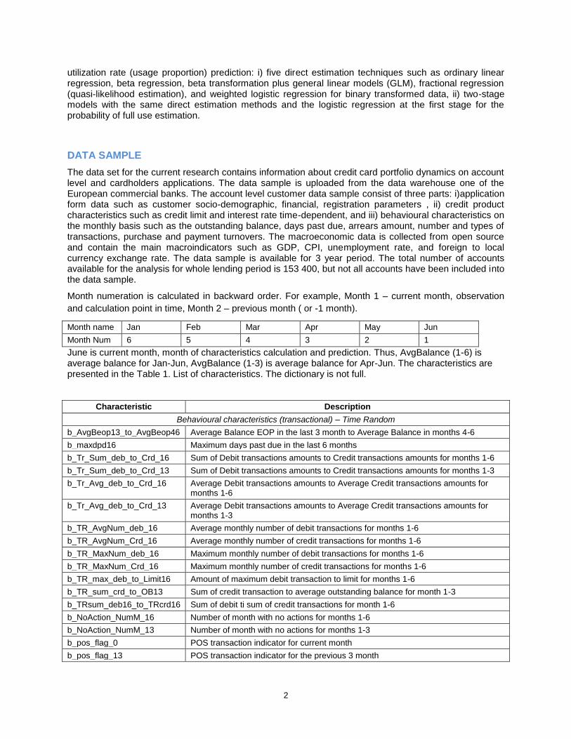
Month numeration is calculated in backward order. For example, Month 1 – current month, observation

and calculation point in time, Month 2 – previous month ( or -1 month).

Month name Jan Feb Mar Apr May Jun

Month Num 6 5 4 3 2 1

June is current month, month of characteristics calculation and prediction. Thus, AvgBalance (1-6) is average balance for Jan-Jun, AvgBalance (1-3) is average balance for Apr-Jun. The characteristics are presented in the Table 1. List of characteristics. The dictionary is not full.

Characteristic Description

Behavioural characteristics (transactional) – Time Random

b_AvgBeop13_to_AvgBeop46 Average Balance EOP in the last 3 month to Average Balance in months 4-6

b_maxdpd16 Maximum days past due in the last 6 months

b_Tr_Sum_deb_to_Crd_16 Sum of Debit transactions amounts to Credit transactions amounts for months 1-6

b_Tr_Sum_deb_to_Crd_13 Sum of Debit transactions amounts to Credit transactions amounts for months 1-3

b_Tr_Avg_deb_to_Crd_16 Average Debit transactions amounts to Average Credit transactions amounts for months 1-6

b_Tr_Avg_deb_to_Crd_13 Average Debit transactions amounts to Average Credit transactions amounts for months 1-3

b_TR_AvgNum_deb_16 Average monthly number of debit transactions for months 1-6

b_TR_AvgNum_Crd_16 Average monthly number of credit transactions for months 1-6

b_TR_MaxNum_deb_16 Maximum monthly number of debit transactions for months 1-6

b_TR_MaxNum_Crd_16 Maximum monthly number of credit transactions for months 1-6

b_TR_max_deb_to_Limit16 Amount of maximum debit transaction to limit for months 1-6

b_TR_sum_crd_to_OB13 Sum of credit transaction to average outstanding balance for month 1-3

b_TRsum_deb16_to_TRcrd16 Sum of debit ti sum of credit transactions for month 1-6

b_NoAction_NumM_16 Number of month with no actions for months 1-6

b_NoAction_NumM_13 Number of month with no actions for months 1-3

b_pos_flag_0 POS transaction indicator for current month

b_pos_flag_13 POS transaction indicator for the previous 3 month

3

Characteristic Description

b_atm_flag_0 ATM transaction indicator for current month

b_atm_flag_13 ATM transaction indicator for the previous 3 month

b_pos_flag_used46vs13 POS transaction in month 4-6 but no transaction in month 1-3

b_pos_flag_use13vs46 POS transaction in month 1-3 but no transaction in month 4-6

b_atm_flag_used46vs13 ATM transaction in month 4-6 but no transaction in month 1-3

b_atm_flag_use13vs46 ATM transaction in month 1-3 but no transaction in month 4-6

No_dpd Flag if account was in delinquency

Application characteristics – Time fixed

Age As of the date of application

Gender Assumption that status constant in time

Education Assumption that status constant in time

Marital status Assumption that status constant in time

Position The position occupied by an applicant

Income As of the date of application

Macroeconomic characteristics – Time random

Unemployment Rate ln lag3 Log of unemployment rate with 3 month lag

GDPCum_ln yoy Log of cumulative GDP year to year to the same month

UAH-EURRate_ln yoy Log of exchange rate of local currency to Euro in compare with the same period of the previous year

CPIYear_ln yoy Log of the ratio of the current Consumer Price Index to the previous year the same period CPI

Table 1. List of characteristics

MODEL BUILDING

The usage of credit limit may be changed during a lifetime period. The utilization rate (Ut) is defined as the outstanding balance (OB) divided by credit limit (L) Ut = OB/L.

Under the assumption that the credit limit is fixed the utilization rate dynamics is completely dependent on the outstanding balance. In current investigation we are concerned with to the utilization rate that is the percentage of the balance relative to a customer credit limit. In our opinion the utilization rate approach is able to give more adequate customer behaviour estimation than direct outstanding balance prediction in sense of consumption habits and customer demand on money, and also is corresponding with bank credit policy.

The credit limit depends on credit policy rules and is defined particularly according to the customer risk profile. The same behavioural customer segments have various outstanding balances correlated particularly with the credit limit. Thus customer segment does not have a typical outstanding balance, but a typical utilization rate as proportion of the credit limit.

The prediction of utilization rate instead of the outstanding balance amount is used to avoid the possible disproportion in behaviour modelling caused by i) different start terms such as bank‟s credit policy and product parameters changes which may affect on the initial credit limit for the same category of customers, ii) hypothesis that credit card customer behaviour is affected mainly by the available balance as part of the credit limit and then by the amount of the available balance.

4

Figure 1. Utilization rate and limit changes

Because of the inconsistencies in the behavioural characteristics calculation (lack of history) and the differences in the utilization rate dynamic at the early and late credit history stages we allocated a separate model for the low MOB period. In our case two periods have been chosen: MOB from 1 to 5 and MOB more than 6. The utilization rate has rapid growth during first 5 month on book showing in Fig.3, but after a peak at 6-8 month on book it stabilized and had slight monotonic decrease.

Figure 2. Average utilization rate depending on Month on Book

As it can been seen from the Figure 3. The utilization rate distribution slightly less than 20% of the observations have the utilization rate from 0% to 5% and approximately 20% of observations have the utilization rate from 95% to 100%. Other cases are distributed almost uniformly from 5% to 80%, and the slight increase of the observations can be observed after 85% rate value. However, in 5% cases, the utilization rate exceeds one hundred percent indicates that the use of loan funds is higher than the set credit limit. This can be explained by i) credit overlimit of the outstanding balance; ii) technical accrual of the interest rates, fees and commissions on the principal account. For the further analysis purposes this cases are replaced by 100% utilization to avoid misinterpretation of the utilization rate and according to the business logic. However, the set of cases can be allocated as a separate category to investigate the reasons and drivers of the credit overlimit.

Cre

dit Lim

it =

10

00

500

Ut Rate

= 50%

Cre

dit Lim

it =

20

00

1000

Ut Rate

= 50%

0

0.2

0.4

0.6

0.8

1

1 3 5 7 9 11 13 15 17 19 21 23 25 27 29

Uti

lizat

ion

Rat

e

Month on Book

Average Utilization Rate by Month on Book

5

Figure 3. The utilization rate distribution

Figure 4. The Utilization Rate, balance and limit distribution by Position type (example) shows the examples of dependence between utilization rate and client characteristics. Top managers have the highest limits, but the lowest utilization rate in compare with other positions. This means that the outstanding balance is not as different as the credit limit.

Figure 4. The Utilization Rate, balance and limit distribution by Position type (example)

METHODOLOGY AND MODELS

We apply five proportions prediction methods for the utilization rate both for one-stage and two-stage models. They are the following:

i) linear regression (OLS)

ii) fractional regression (quasi-likelihood)

iii) beta-regression (non-linear)

0%

5%

10%

15%

20%

25%0

-0.0

5

0.1

-0.1

5

0.2

-0.2

5

0.3

-0.3

5

0.4

-0.4

5

0.5

-0.5

5

0.6

-0.6

5

0.7

-0.7

5

0.8

-0.8

5

0.9

-0.9

5 >1

Utilization rate

The Utilization Rate distribution for active accounts

00.10.20.30.40.50.6

0

5000

10000

15000

Uti

lizat

ion

rat

e

Bal

ance

an

d L

imit

, am

ou

nt

Utilization rate, average balance and limit by client position

avg_limit avg_balance avg_UT

6

iv) beta-transformation + OLS/GLM;

v) weighted logistic regression with data binary transformation.

This section describes methods overview and used SAS code. The comparative analysis of results is presented in the section „Modelling results‟.

LINEAR MODEL BASED APPROACH

The linear regression is tested for proportion modelling (Belotti and Crook, 2012; Arsova et al, 2011)

We assume the utilization rate depends on behavioural, application, macroeconomic characteristics, and also on the previous periods utilization rate with time lag.

mt

M

m

ai

L

l

a

K

k

bitbltinTit MABUTUT

1

11

φ, α, β, γ are regression coefficients (slopes)

Bbit is behavioural factor b for case i in period t, for example, average balance to maximum balance, maximum debit turnover to average outstanding balance, maximum number days in delinquency – time varying;

Aai is application factor a for case i, for example, client‟s demographic, financial and product characteristics such as age, education, position, income, property, interest rate – time constant;

Mmt is macroeconomic factor m in period t such as GDP, FX, Unemployment rate changes – time varying;

UTi t+T is the utilization rate for case i in period t;

l is time lag between current point in time and characteristics calculation slice;

T is the period of prediction in months.

However, time parameter t for this task is used to identify the point in time for lag an each behavioural characteristics and in case the cross sectional analysis the behavioural characteristics and macroeconomic variables are not time varying.

One of the weaknesses of the linear regression application for the utilization rate modelling is the unlimited range of the function outcome. It can be fixed with the conditional function as the following

1,1

1;0,

0,0

xf

xfxf

xf

xf

Linear regression approach can be a reason of high concentration of the rate values on bounds 0 and 1. Moreover, such shape of the distribution function is not continuous and has broken points of inflection what is often non-corresponding with real economic processes. However, this approach is easy to use and it can be applied for quick preliminary analysis of correlations and general trends.

Hereinafter SAS code describe step-by-step all stages of the modelling with the same data source, target and predictors.

7

/* Predictors variable setup */

%let RegAMB_nl =

mob

Limit

UT0

avg_balance

b_AvgOB16_to_MaxOB16_ln

...

CPI_lnqoq_6

SalaryYear_lnyoy_6

;

/* Ordinary Least Squares */

proc reg data=DevSample outest = Est_OLS;

model Target_UT_plus6 = &RegAMB_nl / tol vif collin corrb;

output p=UT_plus6_OLS out=DevSample_pred;

run;

BETA-REGRESSION APPROACH

One of the ways to set bounds for target variable is to apply a transformation of the empirical distribution to the theoretical with appropriate limits. A beta distribution can be applied to match the distribution shape with borders, in our case it is 0 and 1. The approach proposed by Ferrari and Cribari - Neto (2004) for LGD modelling is applied for the utilization rate prediction.

The Beta-distribution can be bounded between two values and parameterized by two positive parameters, which define the shape of the distribution. Generally the empirical probability density function

of the utilization rate distribution is U-shape. The parameters and β should be set up to match the density function shape to minimize the residuals between the empirical and theoretical distribution.

The beta distribution probability density function is

where , β > 0.

The parameters and β are estimated to match the theoretical distribution close to empirical one. Beta distribution function can be represented via Gamma function as

Because the outcome is in the range between 0 and 1 the logistic transformation is used to find the dependences between predictors x(a) and regressor

Log-likelihood function is the following:

ttttttttt yyl 1log11log11logloglog,

8

/* Beta regression */

/* Predictors equation for PROC NLMIXED */

%let eta_nl_beh =

b0+

mob_e*mob+

Limit_e*Limit+

UT0_e*UT0+

...

CPI_lnqoq_e*CPI_lnqoq+

SalaryYear_lnyoy_e*SalaryYear_lnyoy;

%let prm_nl_beh =

b0 = 0

mob_e=0

Limit_e=0

UT0_e=0

...;

proc nlmixed data = DevSample;

parms &prm_nl_beh;

mu = exp(&eta_nl_beh)/(1 + exp(&eta_nl_beh));

phi = exp(d0);

w = mu*phi;

t = phi - mu*phi;

ll = lgamma(w+t) - lgamma(w) - lgamma(t) + ((w-1)*log(Target_UT_plus6_p)) +

((t-1)*log(1 - Target_UT_plus6_p));

model Target_UT_plus6_p ~ general(ll);

predict mu out=betareg_result_nl_beh_mu (keep=Target_UT_plus6_p pred);

predict phi out=betareg_result_nl_beh_phi (keep=Target_UT_plus6_p pred);

run;

The inverse beta-transformation with cumulative distribution function is applied to find real rate value according to the estimated one. After this transformation the logistic regression is applied to estimate dependence between beta-function and predictors, and then inverse transformation from cumulative probability function is applied to get the utilization rate.

BETA-TRANSFORMATION PLUS OLS

The algorithm uses the beta distribution to transform the original target. First stage is to find the beta-distribution coefficients (alpha and beta) to fit the development sample distribution using the non-linear regression procedures. Secondly, replace real target variable by the ideal beta-distributed. Thirdly, find appropriate normal distributed value. Then, run OLS or Generalized Linear Mixed Model to find regression coefficients. After this stage it is need to perform the inverse transformation for normal distribution and then inverse for the beta regression. To obtain a prediction it is necessary to transform linear regression results with normal and then beta regression with the constant alpha and beta coefficient found at the first stage.

/* Beta Transformation PLUS OLS */

proc sql;

create table test_MM_Est as

select *,

samp_mean*(samp_mean*(1-samp_mean)/samp_var-1)as alpha_moments,

(1-samp_mean)*(samp_mean*(1-samp_mean)/samp_var-1) as

beta_moments

9

from

(select mean(Target_UT_plus6_p) as samp_mean,

var(Target_UT_plus6_p) as samp_var

from DevSample);

run;

proc nlmixed data=&r.Tr_plus6m_nl_beh;

/*using MM estimates as starting points*/

parms /bydata data=test_MM_Est(drop=samp_mean samp_var

rename=(alpha_moments=alpha_mle

beta_moments=beta_mle));

ll=log(gamma(alpha_mle+beta_mle))-log(gamma(alpha_mle))-

log(gamma(beta_mle))

+(alpha_mle-1)*log(Target_UT_plus6_p)+(beta_mle-1)*log(1-

Target_UT_plus6_p);

model Target_UT_plus6_p~general(ll);

run;

/* Put alpha and beta for Beta distribution from PROC NLMIXED results */

%let alpha = 0.2909;

%let beta = 0.3049;

/* Transform to Beta distribution */

data DevSample;

set DevSample;

Target_UT_plus6_p_beta = cdf("BETA", Target_UT_plus6_p, &alpha, &beta);

run;

/* Find quantile for Normal distribution for Beta distribution value */

data DevSample;

set DevSample;

Target_UT_plus6_p_beta_prob = quantile("NORMAL", Target_UT_plus6_p_beta);

run;

/* Run GLIMMIX or REG procedures */

proc glimmix data=DevSample;

model Target_UT_plus6_p_beta_prob = &RegAMB_nl;

output out = DevSample pred=Target_UT_plus6_p_beta_prob_pr;

run;

/*or*/

proc reg data=DevSample;

model Target_UT_plus6_p_beta_prob = &RegAMB_nl;

output out = DevSample pred=Target_UT_plus6_p_beta_ols;

run;

/* Inverse transformation from Normal to Beta distribution for results*/

data DevSample;

set DevSample;

Target_UT_plus6_p_beta_prob_res =

quantile("BETA",cdf("NORMAL",Target_UT_plus6_p_beta_prob_pr),&alpha,&beta);

run;

10

Beta transformation approaches widely used for LGD modelling, but empirical researches show not high predictive power results (Arsova et al., 2011; Loterman et al., 2012; Bellotti and Crook, 2009).

UTILIZATION RATE MODELLING WITH FRACTIONAL LOGIT TRANSFORMATION (QUASI-LIKELIHOOD)

The utilization rate is bounded between 0 and 1 and required appropriate methods to keep the predicted value in this range. One of the techniques is fractional logit regression proposed by Papke & Wooldridge (1996). The Bernoulli log-likelihood function is given by

The quasi-likelihood estimator of β is obtained from the maximization of

Crook and Bellotti (2009) apply the Fractional logit transformation for the Loss Given Default parameter modelling:

where RR – is recovery rate.

The LGD parameter has the same features as the Utilizaiton rate such as U-shape and bimodal distribution. Thus the similar techniques can be applied for the modelling and parameters estimations.

The utilization rate UT is transformed to UTTR for regression estimation

UTUTUTTR 1lnln .

The inverse transformation of the predicted value is the following:

TR

TR

UT

UTUT

exp1

exp

The quasi-likelihood methods used to estimate the parameters in the model.

The SAS procedure GLIMMIX is used for the regression coefficients estimation. Procedure GLIMMIX performs estimation and statistical inference for generalized linear mixed models (GLMMs). A generalized linear mixed model is a statistical model that extends the class of generalized linear models (GLMs) by incorporating normally distributed random effects.

11

/*Fractional regression with Quasi-likelihood methods */

/* Preparation for fractional - quasi-likelihood regression */

if Target_UT_plus6 = 0 then Target_UT_plus6_p = 0.0001;

else if Target_UT_plus6 = 1 then Target_UT_plus6_p = 0.9999;

else Target_UT_plus6_p = Target_UT_plus6;

Target_UT_plus6_log=log(Target_UT_plus6_p)-log(1-Target_UT_plus6_p);

proc glimmix data=DevSample;

_variance_ = _mu_**2 * (1-_mu_)**2;

model Target_UT_plus6_p = &RegAMB_nl / link=logit;

output out=DevSample pred(ilink)=ut0_quasi_pred;

run;

Alternatively can be used PROC NLMIXED for fractional response from Yao(2014)

as following:

Program 2. Fractional response regression

proc nlmixed data=MyData tech=newrap maxiter=3000 maxfunc=3000 qtol=0.0001;

parms b0-b14=0.0001;

cov_mu=b0+b1*Var1+b2*Var2+…+b14*Var14;

mu=logistic(cov_mu);

loglikefun=RR*log(mu)+(1-RR)*log(1-mu);

model RR~general(loglikefun);

predict mu out=frac_resp_output (keep=instrument_id RR pred);

run;

WEIGHTED LOGISTIC REGRESSION WITH BINARY TRANSFORMATION APPROACH

The relatively innovative approach is the use of the weighted logistic regression with binary transformation of the data sample. The logit function is bounded between 0 and 1 and traditionally applied for the probability prediction. To apply logistic regression which used binary distribution the target proportion variable need to be transformed from continuous to binary form. The utilization rate can be considered as the probability to use the credit limit by 100%. For example, the utilization rate 75% can be presented as 75% probability to use full credit limit and 25% probability not to use the credit limit. This approach is used by Siddiqi (2012) for the Loss Given Default prediction. Each observation is presented as two observations (or two rows) with the same set of predictors according to the good/bad or 0/1 definition used in logistic regression. The outcome with target 1 corresponds to the rate r, which determines the weight equal to this rate r. The outcome with target 0 corresponds to the rate 1-r, which determines the weight equal to 1-r. The logistic regression probability of event is the utilization rate estimation.

The data sample is transformed according to the following scheme:

Utilization Rate Binary recovery – target Weight

1 1 1

0 0 1

R, 0<r<1 1 r

0 1-r

The set of methods is used for the rates modelling as LGD account level prediction. Stoyanov (2009) investigated, in particular, the following approaches to LGD account level modelling as binary transformation of the LGD using uniform random numbers, binary transformation of the LGD using manual cut-off. Arsova et al (2011) applied both direct approaches to the LGD modelling such as OLS

12

regression, beta regression and fractional regression and indirect approaches such as logistic regression with binary transformation of LGD by random number, logistic regression with binary transformation of LGD by weights, and also multi-stage models like Ordinal Logistic Regression with nested Linear Regression.

This study uses weighted logistic regression with binary transformed sample for rate estimations. In common logistic regression matches the log of the probability odds by a linear combination of the characteristic variables as

T

i

i

i

ip

pp xβ

0

1lnlogit ,

where

pi is the probability of particular outcome, β0 and β are regression coefficients, x are predictors.

,|1Pr,| iiiii YYEP xx is the probability of event for ith observation.

In general this approach can be interpreted as the following: the utilization equal to 10% is the same as from accounts 10 accounts have utilization equal 100% and 90 accounts have utilization equal 0%. Thus the weighted logistic regression with proportions transformed to weights can be applied in SAS/STAT.

/*Weighted Logistic Regression with data sample binary transformation */

/* --- Create binarized sample --- */

/* Development Sample Binary Tranformation*/

data DevSample_wb;

set DevSample;

good=0;

bad=1;

ut_weight=Target_UT_plus6; run;

data DevSample_wb_ne;

set DevSample;

good=1;

bad=0;

ut_weight=1-Target_UT_plus6; run;

data DevSample_wb_reg;

set DevSample_wb DevSample_wb_ne; run;

/* --- Run Model --- */

proc logistic data=DevSample_wb_reg outest = r_Ut_wb_est;

model good = &RegAMB_nl /

selection = stepwise

slentry = 0.05

slstay = 0.05;

output out=r_ut_wb_out predicted=pr_ut;

weight ut_weight; run;

/* Extract real sample for analysis - drop doubles after binary

transformation step */

data wlog_nl_dev (keep = Target_UT_plus6_p pr_ut);

set r_ut_wb_out;

if good=0; run;

13

The predicted outcome from the logistic regression is used as the utilization rate estimation. For validation purposes we need to come back to original data set by dropping the doubled rows (account). For example, if we define the full utilization as „bad = 1‟ and „good=0‟ we need to keep this cases in sample and drop „good=1‟ cases where the outcome estimation is equal to the 1-utilization rate.

MODELLING RESULTS

ONE-STAGE MODELLING APPROACHES SUMMARY

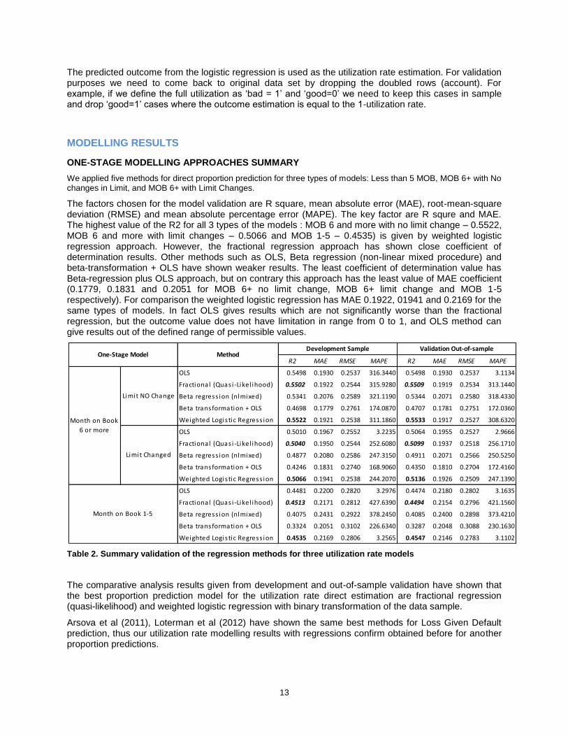
We applied five methods for direct proportion prediction for three types of models: Less than 5 MOB, MOB 6+ with No changes in Limit, and MOB 6+ with Limit Changes.

The factors chosen for the model validation are R square, mean absolute error (MAE), root-mean-square deviation (RMSE) and mean absolute percentage error (MAPE). The key factor are R squre and MAE. The highest value of the R2 for all 3 types of the models : MOB 6 and more with no limit change – 0.5522, MOB 6 and more with limit changes – 0.5066 and MOB 1-5 – 0.4535) is given by weighted logistic regression approach. However, the fractional regression approach has shown close coefficient of determination results. Other methods such as OLS, Beta regression (non-linear mixed procedure) and beta-transformation + OLS have shown weaker results. The least coefficient of determination value has Beta-regression plus OLS approach, but on contrary this approach has the least value of MAE coefficient (0.1779, 0.1831 and 0.2051 for MOB 6+ no limit change, MOB 6+ limit change and MOB 1-5 respectively). For comparison the weighted logistic regression has MAE 0.1922, 01941 and 0.2169 for the same types of models. In fact OLS gives results which are not significantly worse than the fractional regression, but the outcome value does not have limitation in range from 0 to 1, and OLS method can give results out of the defined range of permissible values.

Table 2. Summary validation of the regression methods for three utilization rate models

The comparative analysis results given from development and out-of-sample validation have shown that the best proportion prediction model for the utilization rate direct estimation are fractional regression (quasi-likelihood) and weighted logistic regression with binary transformation of the data sample.

Arsova et al (2011), Loterman et al (2012) have shown the same best methods for Loss Given Default prediction, thus our utilization rate modelling results with regressions confirm obtained before for another proportion predictions.

R2 MAE RMSE MAPE R2 MAE RMSE MAPE

OLS 0.5498 0.1930 0.2537 316.3440 0.5498 0.1930 0.2537 3.1134

Fractional (Quas i -Likel ihood) 0.5502 0.1922 0.2544 315.9280 0.5509 0.1919 0.2534 313.1440

Beta regress ion (nlmixed) 0.5341 0.2076 0.2589 321.1190 0.5344 0.2071 0.2580 318.4330

Beta transformation + OLS 0.4698 0.1779 0.2761 174.0870 0.4707 0.1781 0.2751 172.0360

Weighted Logis tic Regress ion 0.5522 0.1921 0.2538 311.1860 0.5533 0.1917 0.2527 308.6320

OLS 0.5010 0.1967 0.2552 3.2235 0.5064 0.1955 0.2527 2.9666





OLS 0.4481 0.2200 0.2820 3.2976 0.4474 0.2180 0.2802 3.1635





Month on Book 1-5

One-Stage Model MethodDevelopment Sample Validation Out-of-sample

Month on Book

6 or more

Limit NO Change

Limit Changed

14

We provide the detailed results for Limit No Change model. For Limit Change and MOB 1-5 models the distributions and proportions keep similar trends and mainly differ in scales only.

Statistic OLS Fractional Beta

regression Beta+OLS

Weighted Logistic

Regrssion

Mean 0.53520 0.53893 0.50482 0.53220 0.53516

Std Deviation 0.28105 0.28297 0.25019 0.37851 0.28243

Skewness -0.36165 -0.34751 -0.26532 -0.23848 -0.35561

Uncorrected SS 76937 78008 66833 89795 77090

Coeff Variation 52.5123 52.5070 49.5595 71.1215 52.7744

Sum Observations 112680 113465 106284 112048 112671

Variance 0.07899 0.08007 0.06259 0.14327 0.07976

Kurtosis -1.19212 -1.37168 -1.35845 -1.59755 -1.35032

Corrected SS 16630 16859 13178 30163 16793

Std Error Mean 0.00061 0.00062 0.00055 0.00082 0.00062

Table 3. Statistic parameters for predicted distributions for Limit NO Change Model

As it can be seen the mean values are around the 0.53 value for all approaches exclude beta regression which has in average underestimated results. On the other hand Beta transformation with OLS shows the highest standard deviation and variation.

Quantile OLS Fractional Beta

regression Beta+OLS

Weighted Logistic

Regrssion

100% Max 1.1187 0.9821 0.9495 1.0000 0.9829

99% 0.9440 0.9251 0.8713 0.9962 0.9188

95% 0.8960 0.8845 0.8287 0.9789 0.8804

90% 0.8647 0.8626 0.8053 0.9663 0.8581

75% Q3 0.7843 0.7987 0.7346 0.9079 0.7940

50% Median 0.5985 0.6153 0.5543 0.6285 0.6103

25% Q1 0.2753 0.2551 0.2608 0.0997 0.2568

10% 0.1177 0.1152 0.1333 0.0057 0.1103

5% 0.0770 0.0904 0.1143 0.0025 0.0850

1% -0.0045 0.0562 0.0872 0.0007 0.0446

0% Min -0.3780 0.0055 0.0232 0.0000 0.0018

Table 4. Outcome Distributions for five prediction methods for Limit NO Change Model

The predicted with OLS utilization rate distribution has U-shape with some values below zero and higher than 1 (see Figure 5. Linear regression predicted outcome distribution). To avoid the values out of interval without use of conditional function like if value less than 0 let it be 0 we apply another approaches with outcome values in range.

Four other approaches have outcome values strictly between 0 and 1. Figure 6. Beta regression, Beta-transformation, Fractional regression, and Weighted logistic regression distributions. The U-shape distribution corresponds with original utilization rate distribution in the data sample. However, at the right side (high proportion values) pick is not in the value 1 as expected, but in the area of 0.85-0.9 what has made the prediction biased. Beta regression (NLMIX) distribution is similar to fractional one but the left pick of low utilization is higher than the area of high utilization. This means that the prediction can be underestimated. The U-shape of the beta-transformation approximated with OLS has the most fitted shape with the original distribution. However, the validation results are weakest among all models (Table 2. Summary validation of the regression methods for three utilization rate models). An approach with weighted logistic regression also has right peak not at the high bound, but in 0.85-0.9 area. The predicted outcome can be underestimated for high utilization values, but the statistical validation results have shown the best values. Weighted logistic and Fractional response regressions give similar distributions and higher predictive power in compare with other approaches.

15

Figure 5. Linear regression predicted outcome distribution

Beta regression

Beta transformation + OLS

Fractional regression (quasi-likelihood)

Weighted Logistic Regression

Figure 6. Beta regression, Beta-transformation, Fractional regression, and Weighted logistic regression distributions

16

Parameter

Estimate

Standard

errort Value Pr > |t|

Parameter

Estimate

Standard


Parameter

Estimate

Standard


Intercept 0.19868 0.00823 24.14 <.0001 0.14837 0.01252 11.85 <.0001 0.2773 0.0156 17.78 <.0001

Account info

mob -0.00328 0.0001604 -20.44 <.0001 -0.00188 0.0002648 -7.09 <.0001

limit 1.59E-07 1.33E-07 1.19 0.2345 -2.7E-06 2.31E-07 -11.67 <.0001 -2.4E-06 2.93E-07 -8.2 <.0001

UT 0.53061 0.00312 170.19 <.0001 0.51333 0.00492 104.28 <.0001 0.43759 0.00581 75.3 <.0001

avg_balance 2.07E-06 2.37E-07 8.73 <.0001 3.84E-06 3.57E-07 10.74 <.0001 0.0000032 5.61E-07 5.7 <.0001

Behavioural - dynamic

b_AvgOB16_to_MaxOB16_ln 0.04088 0.00134 30.59 <.0001 0.04039 0.00233 17.34 <.0001

b_TRmax_deb16_To_Limit_ln 0.00699 0.00049122 14.22 <.0001 0.01649 0.0008275 19.93 <.0001 -0.00552 0.00045667 -12.09 <.0001

b_TRavg_deb16_to_avgOB16_ln -0.01841 0.00068774 -26.76 <.0001 -0.03006 0.00125 -24.08 <.0001 -0.01085 0.00105 -10.31 <.0001

b_TRsum_deb16_to_TRsum_crd16_ln 0.01087 0.00061894 17.55 <.0001 0.01241 0.00119 10.46 <.0001 0.02698 0.00074873 36.04 <.0001

b_UT1_to_AvgUT16ln -0.00282 0.00040175 -7.01 <.0001 -0.00195 0.0006926 -2.82 0.0048 0.00912 0.00068481 13.32 <.0001

b_UT1to2ln 0.00178 0.00030936 5.76 <.0001 0.0009643 0.0005288 1.82 0.0682 -0.00734 0.00021089 -34.79 <.0001

b_UT1to6ln -0.0048 0.00025297 -18.99 <.0001 -0.00647 0.0004217 -15.34 <.0001

b_NumDeb13to46ln 0.00545 0.00033788 16.14 <.0001 0.00937 0.0006162 15.21 <.0001

b_inactive13 0.0824 0.00464 17.77 <.0001 0.16916 0.00812 20.84 <.0001

b_avgNumDeb16 0.0001071 0.00004173 2.57 0.0103 -0.00149 0.0003031 -4.91 <.0001 0.00679 0.00034267 19.83 <.0001

b_OB_avg_to_eop1ln -0.00132 0.00033009 -4 <.0001 -0.000629 0.00052 -1.21 0.2262 -0.00927 0.00064119 -14.45 <.0001

b_DelBucket16 0.02571 0.00235 10.96 <.0001 0.03251 0.00441 7.36 <.0001 0.02082 0.00821 2.54 0.0112

b_pos_flag_0 0.01847 0.00174 10.63 <.0001 0.01697 0.00244 6.94 <.0001 0.021 0.00263 7.99 <.0001

b_pos_flag_13 0.03935 0.00213 18.51 <.0001 0.04299 0.003 14.32 <.0001

b_atm_flag_0 0.053 0.00152 34.91 <.0001 0.05427 0.00213 25.44 <.0001 0.09135 0.00279 32.7 <.0001

b_atm_flag_13 0.05824 0.00246 23.7 <.0001 0.03996 0.00355 11.25 <.0001

b_pos_flag_used46vs13 0.02783 0.0019 14.64 <.0001 0.02612 0.0027 9.68 <.0001

b_pos_flag_use13vs46 -0.02589 0.00203 -12.78 <.0001 -0.03041 0.00286 -10.61 <.0001

b_atm_flag_used46vs13 0.01634 0.0022 7.43 <.0001 0.00351 0.00329 1.07 0.2861

b_atm_flag_use13vs46 -0.02562 0.00214 -11.96 <.0001 -0.01679 0.00306 -5.48 <.0001

b_pos_use_only_flag_13 0.01185 0.00275 4.31 <.0001 0.00375 0.00397 0.95 0.3441 -0.03498 0.0047 -7.45 <.0001

no_dpd -0.00524 0.00413 -1.27 0.2039 0.00506 0.00694 0.73 0.4657

max_dpd_60 0.02693 0.00698 3.86 0.0001 0.03216 0.01178 2.73 0.0063

Application- static

AgeGRP1 0.01494 0.00189 7.9 <.0001 0.01191 0.0025 4.77 <.0001 0.02992 0.00353 8.47 <.0001

AgeGRP3 -0.00166 0.00172 -0.97 0.3323 0.00783 0.00234 3.34 0.0008 -0.01675 0.0032 -5.23 <.0001

customer_income_ln -0.03324 0.00165 -20.1 <.0001 -0.02355 0.00258 -9.11 <.0001 -0.04541 0.00327 -13.87 <.0001

Edu_High -0.02094 0.00175 -11.94 <.0001 -0.0196 0.00249 -7.86 <.0001 -0.04343 0.00326 -13.33 <.0001

Edu_Special -0.00198 0.00169 -1.17 0.2415 -0.00226 0.00243 -0.93 0.3518 -0.01095 0.00314 -3.48 0.0005

Edu_TwoDegree -0.01803 0.00389 -4.63 <.0001 -0.01047 0.00539 -1.94 0.052 -0.0494 0.00731 -6.76 <.0001

Marital_Civ 0.00494 0.00268 1.84 0.0653 0.00403 0.0038 1.06 0.2898 0.03416 0.00501 6.82 <.0001

Marital_Div 0.00377 0.0019 1.98 0.0478 0.00829 0.00279 2.97 0.003 0.02359 0.00352 6.71 <.0001

Marital_Sin 0.00625 0.00201 3.11 0.0019 0.00631 0.00282 2.24 0.0253 0.019 0.00376 5.06 <.0001

Marital_Wid 0.02133 0.00349 6.12 <.0001 0.03034 0.00613 4.95 <.0001 0.03118 0.00642 4.85 <.0001

position_Man 0.01174 0.00183 6.43 <.0001 0.01479 0.00272 5.45 <.0001 0.01727 0.00342 5.06 <.0001

position_Oth 0.00891 0.00181 4.91 <.0001 0.00718 0.00257 2.79 0.0052 0.00821 0.00337 2.43 0.015

position_Tech 0.00673 0.0017 3.96 <.0001 0.01045 0.00245 4.26 <.0001 0.01417 0.00315 4.49 <.0001

position_Top 0.00989 0.00336 2.94 0.0033 0.01065 0.00568 1.87 0.0611 0.00769 0.00629 1.22 0.2211

sec_Agricult 0.00428 0.00327 1.31 0.1905 0.01956 0.00485 4.03 <.0001 -0.0196 0.00608 -3.22 0.0013

sec_Constr -0.00428 0.00437 -0.98 0.3279 -0.0252 0.00651 -3.87 0.0001 -0.01599 0.00802 -2 0.046

sec_Energy -0.00213 0.00281 -0.76 0.4483 -0.00362 0.00401 -0.9 0.3664 -0.00917 0.00522 -1.76 0.0792

sec_Fin -0.02624 0.00211 -12.45 <.0001 -0.03388 0.00316 -10.72 <.0001 -0.04477 0.00388 -11.55 <.0001

sec_Industry 0.00344 0.00552 0.62 0.5328 0.00516 0.008 0.64 0.5195 -0.000521 0.01043 -0.05 0.9602

sec_Manufact 0.00805 0.0043 1.87 0.0613 0.00217 0.00622 0.35 0.7266 -0.02594 0.00785 -3.3 0.001

sec_Mining 0.00362 0.00299 1.21 0.2259 0.00344 0.00436 0.79 0.4303 0.01126 0.00563 2 0.0456

sec_Service -0.00867 0.00158 -5.49 <.0001 -0.01918 0.00232 -8.27 <.0001 -0.01405 0.00296 -4.75 <.0001

sec_Trade -0.00604 0.00212 -2.84 0.0045 -0.00638 0.003 -2.13 0.0332 -0.00529 0.00395 -1.34 0.18

sec_Trans -0.00676 0.00414 -1.63 0.1026 -0.01358 0.00608 -2.23 0.0256 -0.01666 0.00761 -2.19 0.0286

car_Own -0.01099 0.0015 -7.34 <.0001 -0.00857 0.00219 -3.91 <.0001 -0.01934 0.00279 -6.93 <.0001

car_coOwn 0.00212 0.00228 0.93 0.3517 0.00259 0.00332 0.78 0.4353 -0.00269 0.00425 -0.63 0.5277

real_Own 0.0005113 0.00145 0.35 0.7248 0.00244 0.00205 1.19 0.2341 -0.00849 0.00269 -3.15 0.0016

real_coOwn -0.00257 0.00154 -1.68 0.0939 -0.00185 0.00214 -0.87 0.3866 0.00291 0.00286 1.02 0.3097

reg_ctr_Y -0.00803 0.00223 -3.6 0.0003 -0.01008 0.00316 -3.19 0.0014 -0.00798 0.00256 -3.12 0.0018

reg_ctr_N -0.00653 0.00224 -2.92 0.0035 -0.00913 0.00318 -2.87 0.0041 0.00625 0.00419 1.49 0.1358

child_1 0.01064 0.0019 5.61 <.0001 0.01041 0.00266 3.91 <.0001 0.0208 0.00356 5.84 <.0001

child_2 0.0065 0.00108 6.02 <.0001 0.00441 0.00157 2.8 0.0051 0.01498 0.00203 7.39 <.0001

child_3 0.03175 0.00362 8.78 <.0001 0.02034 0.00564 3.61 0.0003 0.03036 0.00672 4.52 <.0001

Macroeconomic - dynamic

Unempl_lnyoy_6 0.26643 0.02401 11.1 <.0001 0.52425 0.03853 13.61 <.0001 0.57361 0.14279 4.02 <.0001

UAH_EURRate_lnmom_6 -0.07515 0.02953 -2.54 0.0109 -0.09468 0.04392 -2.16 0.0311 -0.61495 0.0459 -13.4 <.0001

UAH_EURRate_lnyoy_6 0.16824 0.0185 9.09 <.0001 0.19912 0.02704 7.37 <.0001 0.22877 0.04324 5.29 <.0001

CPI_lnqoq_6 0.62416 0.04887 12.77 <.0001 1.46551 0.07027 20.86 <.0001 -0.60753 0.07393 -8.22 <.0001

SalaryYear_lnyoy_6 -0.26247 0.04234 -6.2 <.0001 0.13688 0.06107 2.24 0.025 0.01177 0.08418 0.14 0.8888

Credit Limit Changes

l_ch1_ln (limit change month ago) 0.05093 0.00673 7.57 <.0001

l_ch6_ln (limit change 6 month ago) 0.09616 0.00382 25.17 <.0001

MOB 6+ - Limit NO Change MOB 6+ - Limit Changed MOB 1-5

Characteristic

Table 5. Parameters estimation comparative analysis for Ordinary Least Squares example

17

Models for APP, BEH NL and BEH CL used different sets of characteristics is shown in Table 5. Parameters estimation comparative analysis for Ordinary Least Squares example. The application parameters are used for all segments, but long term behavioural predictors are not used for APP and limit changes are used for BEH CL only. We provide OLS method estimations here for the comparative analysis of the model segments. As it can be seen from the table 4 the same characteristics have different estimations and t-values for APP, BEH NL and BEH CL. For example, current utilization rate is less significant for limit changed account than for the account without limit changes (170 and 104 t values respectively). Some characteristics can have opposite trend for behavioural and application model such as education level and the indicator of the POS use only for the last 3 month. Thus the same drivers impact on the utilization rate and customer behaviour in the different way.

TWO-STAGE MODEL SUMMARY

Two-stage model means that at the first stage the probability to get a boarder value as 0 and 1 is calculated, and then the proportion estimation in the interval (0;1) are applied.

At the first stage the probability that an account has zero utilization (Pr (Ut=0) and then that an account has full utilization (Pr (Ut=1)) in the performance period is calculated with binary logistic regression. At the second stage the proportion between 0 and 1 excluding 0 and 1 values is calculated according to the set of the approaches used for one-stage direct estimation (Figure 7. Two-stage regression model schema).

The two-stage model utilization rate is calculated with the following formula:

1,0|1Pr11Pr0Pr1 UtUtUtEUtUtUtUt

Where Pr(Ut=0) and Pr(Ut=1) are the probability the utilization rate is equal to 0 or 1 respectively.

1,0| UtUtUtE is the utilization rate proportion estimation for the utilization rates not equal zero

and not equal to 1.

Figure 7. Two-stage regression model schema

Two-stage model consist of two parts: the probability of zero utilization and full utilization with use of logistic regression and the proportion estimation with use of the set of the same methods as for one-stage model.

In general two-stage models have shown better model accuracy and prediction results for development and validation samples, but the difference in forecasts errors are insignificant. For example, for Limit No Change model for OLS method for one-stage and two-stage approaches R^2 = 0.5498 and 0.5534, MAE= 0.1930 and 0.1913 respectively. However, if we compare Stage 2 model with one-stage direct estimation it can be seen that one-stage model gives better results. For example, one-stage and stage 2 of two-stage model R^2 = 0.5498 and 0.4310, MAE= 0.1930 and 0.1948 respectively. But this difference

Logistic regression 1

Pr(Ut=0|X) vs. x|0Pr Ut

0Ut Logistic regression 2

Pr(Ut=1|(1-Pr(Ut=0|x), x) vs. 1,0Pr Ut

Proportion Estimation: OLS, Fractional, WLR, Beta etc.

1,0Pr|ˆ UtxtU T

1ˆ tU

Partial Utilization| 1-Pr(Ut=1|X) Full Utilization

No Utilization

Some Utilization| 1-P(Ut=0|X)

18

is compensated high prediction performance of the Stage 1 model – logistic regression, which has KS = 0.6262 and 0.5931, GIni = 0.7479 and 0.7243 for probability the utilization rate is equal to zero and the utilization rate is equal to 1 respectively.

Table 6. Two-stage models comparative analysis

The two-stage models for other two segments: Limit Changed and Month on Book less than 6 have shown approximately the same results for models quality assessment and validation. Difference is in scale only. For example, MOB 1-5 model shows low KS and Gini parameters (~0.30 and ~0.40 respectively) what is normal and expected for the application scoring.

CONCLUSION

The main task of this paper is to find more accurate method for the credit limit utilization rate. We applied a number of methods already used for proportions prediction as Loss Given Default and compared obtained results with published. The general proportion models accuracy evaluations for LGD are confirmed for the utilization rate too (Belotti and Crook, 2009; Arsova et al, 2011; Yao et al, 2014). We applied five methods: i) linear regression (OLS), ii) fractional regression (quasi-likelihood), iii) beta-regression (non-linear), iv) beta-transformation + OLS/GLM, v) weighted logistic regression with data binary transformation in one-stage direct model and two-stage model with logistic regression for the probability of bounded values estimation.

The best validation results have been shown by for both one- and two-stage models are:

i) fractional regression and

ii) weighted logistic regression with data binary transformation.

However, OLS results are not differ dramatically and describe the similar distribution shape. Beta transformation has the most similar distribution shape but has the worst validation results.

Two-stage models show slight better result for all five approaches than one-stage model. The probabilities estimation models for the utilization rate bound values 0 and 1 have high performance results for credit risk behavioural models.

We also segmented our population and use three separate groups of models for customer with less than 6 month on balance, customer with 6 and more month on balance and no changes limit, and customer with 6 and more month on balance and increased limit. These three model segment has different sets of characteristics. For example, additional limit changes parameters or limited number of behavioural characteristics for MOB less than 6 accounts. Models for changed limit are slight stronger than MOB 6+

Month on

Book

Limit

ChangesStage Method

Stage 1 Probability KS Gini ROC KS Gini ROC

Pr(UT=0) Logis tic Regress ion 0.6262 0.7479 0.8739 0.6331 0.7547 0.8774

Pr(UT=1) Logis tic Regress ion 0.5931 0.7243 0.8622 0.6036 0.7355 0.8678

Stage 2 Proportion Estimation R2 MAE RMSE MAPE R2 MAE RMSE MAPE

OLS 0.4310 0.1948 0.2462 4.9151 0.4235 0.1950 0.2462 4.8260

Fractional ( Quas i -Likel ihood) 0.4309 0.1946 0.2463 4.9683 0.4235 0.1950 0.2462 4.8260




Two-stage Aggregate R2 MAE RMSE MAPE R2 MAE RMSE MAPE

OLS 0.5534 0.1913 0.2535 3.1366 0.5536 0.1910 0.2526 3.0784

Fractional ( Quas i -Likel ihood) 0.5527 0.1915 0.2536 3.1590 0.5529 0.1912 0.2528 3.0979




Development Sample Validation Out-of-sample

MOB 6 or

more

Limit NO

change

0<UT<1

0<= UT <=1

19

without limit change rather because of additional parameters, models for MOB less than 6 show weaker predictive power because of short behavioural history and these models rather based on application data.

Business contribution is in use of the utilization rate for the profitability estimation in credit limits strategy and marketing strategies at the account level. Credit limit utilization rate depends on the customer behavioural pattern and revolvers and transactors can have different utilization rates.

The next stages of the investigation for the utilization rate modelling can be dedicated to the use of other methods prediction like discrete choice, CHAID, SVM etc. and based on LGD modelling experience can give even higher performance results than regression.

REFERENCES

[1] RamonaK.Z.Heck (1987). Differences in Utilisation Behaviour Among Types of Credit Cards. The Service Industries Journal Volume 7, Issue 1, 1987.

[2] Bellotti T. and Crook J.(2009).Loss Given Default models for UK retail credit cards. CRC working paper 09/1.

[3] Bellotti, T. and Crook, J. (2012). Loss given default models incorporating macroeconomic variables for credit cards. International Journal of Forecasting, 28, 171-182.

[4] Arsova, M. Haralampieva, T. Tsvetanova (2011). Comparison of regression models for LGD estimation. Credit Scoring and Credit Control XII 2011, Edinburgh.

[5] Stefan Stoyanov (2009). Application LGD Model Development. A Case Study for a Leading CEE Bank. Credit Scoring and Credit Control XI Conference, Edinburgh, 26th-28th of August 2009

[6] Steven Xizogang Wang (2001). Maximum weighted likelihood estimation. The University of British Columbia. A part of thesis published, June, 2001.

[7] Sumit Agarwal Brent W. Ambrose Chunlin Liu (2006). Credit Lines and Credit Utilization. Journal of Money, Credit, and Banking, Vol. 38, No. 1 (February 2006).

[8] Papke, L. E. and Wooldridge, J. M. (1996), “Econometric Methods For Fractional Response Variables With an Application to 401(K) Plan Participation Rates”, Journal of Applied Econometrics, vol. 11, 619-632

[9] Ferrari, S. L. P. and Cribari-Neto, F. (2004), “Beta Regression for Modelling Rates and Proportions”, Journal of Applied Statistics, 31, 799-815

[10] Anthony Van Berkel, Bank of Montreal and Naeem Siddiqi (2012). Building Loss Given Default Scorecard Using Weight of Evidence Bins in SAS®Enterprise Miner™. SAS Institute Inc. Paper 141-2012

[11] Xiao Yao, Jonathan Crook, Galina Andreeva. (2014). Modeling Loss Given Default in SAS/STAT®. SAS Forum 2014. Paper 1593-2014.

CONTACT INFORMATION

Your comments and questions are valued and encouraged. Contact the author at:

Denys Osipenko The University of Edinburgh Business School 29 Buccleuch Place, Edinburgh, Lothian EH8 9JS [email protected]

SAS and all other SAS Institute Inc. product or service names are registered trademarks or trademarks of SAS Institute Inc. in the USA and other countries. ® indicates USA registration.

Other brand and product names are trademarks of their respective companies.

Documents

The Comparative Analysis of Predictive Models for …support.sas.com/resources/papers/proceedings15/3328-2015.pdf1 Paper 3328-2015 The Comparative Analysis of Predictive Models for