THE COEFFICIENT PROBLEM IN THE THEORY OF LINEAR … · THE COEFFICIENT PROBLEM IN THE THEORY OF LINEAR PARTIAL DIFFERENTIAL EQUATIONS^) BY ... Z = Xi + iXi, 2* = Xi — tXi, ... onto

THE COEFFICIENT PROBLEM IN THE THEORY OFLINEAR PARTIAL DIFFERENTIAL EQUATIONS^)

BY

STEFAN BERGMAN

1. The basic idea of the application of integral operators to the Weier-

strass-Hadamard direction. In order to generate and investigate solutions of

differential equations, operators p (defined as the integral operators of the

first kind) have been introduced in [2; 6](2). p transforms analytic functions

of one and two variables into solutions of linear elliptic differential equations

of two and three variables, respectively. It has been shown in the above-

mentioned papers that p (as well as some other operators connected with p)

preserves many properties of the functions to which the operator is applied.

This situation permits us to use theorems in the theory of functions to obtain

theorems not merely on harmonic functions in two variables, but on solutions

of other linear differential equations as well(3).

In the present paper the above-mentioned method is used to prove con-

nections between the properties in the large of solutions ip of certain linear dif-

ferential equations, see (1.1) and (1.3), on one side and the structure of cer-

tain subsequences of the coefficients of the series development of \p at the

origin on the other.

Let us formulate these procedures in a somewhat more concrete manner,

at first for equations in two variables. Let ^bea (real) solution of the differ-

ential equation

(1.1) L«0 - *„. + F(z, 2*)^ K — (f n„ + *X2X2) + F(Xl, xM = 0,4

Z = Xi + iXi, 2* = Xi — tXi,

where F(z, z*) = F(xi, x-i) is a (real) entire function(4).

In analogy to the case of harmonic functions we associate with \(/ an

analytic function g of one complex variable z by the relation

(1.2) 4(z, 0) = (g(z) + f(0))/2.

Received by the editors August 17, 1951.

t1) Paper done under contract with the Office of Naval Research N5ori 76/16 NR 043-046.

(2) Numbers in brackets refer to the bibliography at the end of the paper.

(3) The operation Re [p( )] represents a generalization to the case of more general linear

differential equations of the operator Re[ ] (taking of real part). It permits us to generalize

methods in the theory of harmonic functions which are based on the use of the operator Re.

A subscript attached to an operator indicates dimension of the function produced.

(4) I.e., real for real values of the arguments X\, x^, and entire when continued to complex

values of Xi, x¡.

1

License or copyright restrictions may apply to redistribution; see https://www.ams.org/journal-terms-of-use

2 STEFAN BERGMAN (July

(Thus g/2+const. coincides with \p in the so-called characteristic plane,

z* = 0.) g(z) is defined as the C-associate of \p(z, z*) with reference to the

origin. Re [p( )], where p=p2 is the operator of the first kind mentioned

above, transforms g{z) back into the solution \p(z, z*).

The expression Re [p2(g)], representing the solution ^ in terms of its

C-associate, g, involves two integrations, see (2.7), (2.5). The first integration,

see (2.7), transforms g into a function of one complex variable. Due to this

fact various classical results on the relations between analytic functions (in

particular, algebraic functions) on one side, and their integrals on the other,

can be interpreted successfully as theorems on solutions \fi of (1.1). Using these

and other properties of p2 the classical results in the theory of functions yield

among others the following types of theorems:

Let 'R.o be the Riemann surface of an algebraic function, and let SICRo)

be the class of solutions of (1.1) such that the C-associates 2^(z, 0), i/'GSICR.o),

are single-valued on 'R.o- Then every ^GSlCRo) can be represented in the form

of an integral, whose integrand is a product of two expressions. The first

factor depends only on F (i.e., only upon the equation), the second depends

only upon ir\o (i.e., independent of F) and (for all ^GSIô)) can be repre-

sented in a closed form involving algebro-logarithmic expressions, certain

0-functions, their derivatives, and finitely many transcendental functions(6).

Using the classical theorems (Weierstrass, Hadamard, Eisenstein, Pólya,

Szegö, . . . ) it is possible to show that the subsequences {amo}, m=0, 1, 2,

• • -, of the developments \}i = ^,m¡n amnzmz*n, i/'GSICR.o) lie in a certain mani-

fold (which is independent of F) of the coefficient space (§§2, 3).

The study of differential equations in three variables represents a further

step in the development of this approach(6). In continuation of [6; 8], in

the present paper we consider differential equations

(aV/3zî) + (dV/3*î) + (aV/d*î) +Ft = Q,

$ = ii{X), X = (xi, Xi, x3),

where F is an entire function of r2 = JjL x x\. These investigations consist of

two steps: the study (1) of the mappings of harmonic functions \[i(X), onto

algebras, (2) of the transition from the harmonic functions to the solutions of

(1.3) (with FÔ).

(2) proceeds in essentially the same manner as in the two-dimensional

case, and involves mainly technical difficulties. Thus problem (1) is the major

point in this study.

In §4 we discuss the mappings of harmonic functions onto functions of

two complex variables, g(Z, Z*). In analogy to the class 2i(flo) we introduce

(6) This result is a direct application of the representation of integrals of algebraic func-

tions by 0-functions and integrals of the first kind.

(6) Another direction is the study of differential equations with singular coefficients [7; 9],

and quasi-linear equations.


1952J THE COEFFICIENT PROBLEM 3

certain subclasses Sí(ai, • • • , ap; N), see p. 18, of multi-valued harmonic

functions. We show that ip(X)£21 (ai, • • • , ap; N) can be represented in

closed form by algebro-logarithmic expressions, ^-functions, their derivatives,

and finitely many transcendental functions belonging to 2I(ai, • ■ ■ , ap; N).

In §§5 and 6 we show that subsequences of the coefficients of their series de-

velopment at the origin and at infinity belong to certain manifolds of the

coefficient space.

As in the two-dimensional case, these results can be extended to the case

of solutions of equation (1.3). See §7. In particular, we obtain a representation

of solutions 4/&îau • • ■ > Gp', N) of (1.3) in the form of double integrals of

products of two terms. The first term depends only upon F (i.e., the equation

(1.3)) and the second is independent of F and can be represented in a closed

form, in certain cases, by the inverse of the Weierstrass ^-function. Its argu-

ment and parameters are conveniently chosen combinations of the variables.

Further we show that a subsequence of the coefficients of the series develop-

ment of \f/(X) &i(fli, • • • , ap; N) lies in a certain manifold of the coefficient

space, which manifold is independent of F. Finally we mention the possi-

bilities of extending our methods to more general differential equations in

three variables (§8).

We see that due to the particular simple laws of mappings(7) by the

integral operators considered a large variety of results in the theory of

analytic functions may be used to obtain theorems on solutions of differential

equations (1.1) and (1.3). (The theorems 2.2, 7.1, 7.2, etc., are only examples

in this direction.) The main interest of our considerations consists of working

out a method which permits us to extend certain directions in the theory of

functions, namely those dealing with the coefficient problem and classifica-

tion of certain types of solutions, to the theory of equations (1.1) and (1.3).

The author wishes to thank Dr. Henry Pollak for his helpful advice and

aid in the preparation of the present paper, which in some instances led to

a simplification of the presentation.

2. The associate of a solution \[/ of equation (1.1). Solutions whose asso-

ciates of the first kind are algebraic. Let H(xi, x2) = ^(z, z*) be a (real)

harmonic function of two variables; then it can be represented in the form(8)

(') The mappings P of one class of functions, say analytic functions /, onto another class,

say solutions ip of (1.3), are defined at first in the small. Since/and 4> can be continued analyti-

cally, one can extend the definition of the mappings to the large. Since the Riemann surfaces

of the corresponding functions/ and \p do not need to coincide, we must in the latter case indi-

cate the sheet on which the reference point has been chosen, as well as what branch of \p is

obtained by P(/).(8) We note that if xi and xi are real, then z and z* are conjugate to each other; if x\ and

xi are complex, z and z* become two independent variables.

A function ifr(z, z) which for real values of the arguments, X\, x% (or z*=z conjugate to z),

is real, is said to be real. In the sequel <j/ will denote either real or complex solution of the dif-

ferential equation.


4 STEFAN BERGMAN [July

(2.1) \/i(z, z*) - [g(z) + |(z*)]/2, z = Xi + ix2, z* = xi — ix2,

so that

(2.2) g(z) = 24i{z, 0) + const, |(z*) = 2^(0, z*) + const.

Therefore the analytic function g, whose real part is \p, can be obtained by

continuing \p to complex values of the arguments and considering it in the

characteristic plane z* = 0 (or z = 0). In the following, we shall refer to g as the

associate of the first kind ofyp with reference to the point(9) O = (0, 0).

The Weierstrass results on integrals of algebraic functions can be inter-

preted in a form stating that if in the characteristic plane a harmonic func-

tion is an integral of an algebraic function, then it can be represented in the

large by employing the Weierstrass formulas. Obviously various results of

this kind about analytic functions can be stated for harmonic functions.

Various operators have been introduced transforming analytic functions

of a complex variable into solutions of linear partial differential equations of

elliptic type

¿«0 - **«• + A*. + Bf, + 4Ff

(2.3) 1 1= Af + — (A + B)4,x + — (A- B)ty + 4F* = 0.

2 2i

In the present section, we shall show that if A =B=0 and F is an entire

function of z, z*, the above results in the theory of functions of a complex vari-

able can be used to derive similar results for solutions of (1.1)(10). Our con-

siderations are based on the following theorem derived in [2] concerning the

representation of solutions of the differential equation (1.1):

Theorem 2.1. Let E satisfy the differential equation

(2.4) (1 - P)Ez,t - (1/0 Ez. + 2zt{Ezz. + FE) = 0,

and certain additional conditions, then

(2.5) 4i = P2(/) - j E{z, z*, t)f(-z(l - /s))*/(l - t*y<\

where f is an arbitrary function regular at the origin of one complex variable, will

be a {complex) solution of (1.1).

(9) Unless stated to the contrary, we shall assume, in the following, that the associate of

the first kind is taken with reference to the origin, 0. While in the case of harmonic functions in

two variables, the change of the reference point does not change the character of the associate,

the situation is different in the case of differential equations (2.3) and in three variables. One

of the purposes of our considerations is to study solutions whose associates with respect to a

conveniently chosen reference point become particularly simple.

(10) The assumption A=B = 0 was made here only to avoid long formulas. The procedure

can be repeated with almost no changes if A and B do not vanish.


1952] THE COEFFICIENT PROBLEM 5

In [2], it has been shown that for every equation (1.1) there exist various

functions E of the above kind, which are defined as generating functions for

an integral operator P2. In particular, there exists the function E\(z, z*, t)

having the property E\{z, 0, /) =Ei(0, z*, /) = 1, defined as the generating func-

tion of the first kind with the reference point 0.

If E can be written in the form 1 + "^ñ-i t2nQ(n)(z, z*), then the operator

(2.5) can be modified. We can, namely, write instead of (2.5),

(2.6) * = p2(g) m g{z) + ¿ 2-»<2<»>(z, a*)[B(n, n + l)]-^»(a)

where

(2.6a) g

(2.6b) gn(z)

(2.7) /(z)

In the case of integral operators of the first kind, Q(n>(z, 0) =Qln)(0, z*) =0,

»¡£l. In analogy to the situation in the case of harmonic functions, we obtain

for integral operators of the first kind, the same relations (2.2) between a (real)

solution \¡/(z, z*) o/(l.l) and the corresponding associate g of the first kind.

Remark 2.1. Studying complex solutions \¡/(z, z*), z = Xi-H'x2, z* = X\ — ix2,

of (1.1) it is useful to distinguish a special subclass, a, of solutions, namely

those which (when continued to complex values of the arguments) have the

property that in the characteristic plane z = 0 they become constant. In the

case of equation (1.1) solutions generated by the integral operator of the first

kind form the class a. In the special case F = 0, a is the class of analytic func-

tions of a complex variable.

The aim of the present section is to characterize the class of real solutions

of (1.1) which have the property that in the characteristic plane z* = 0, they

become algebraic functions. (In our terminology, we shall say that the asso-

ciate of the first kind of \p is an algebraic function. See also footnote 9.) In

the case where F = 0 (i.e., in the case of Laplace's equation) the harmonic

function with an algebraic associate is an algebraic function of z, z*, which is

defined on a certain Riemann surface, say ÍV The theory of integral oper-

ators permits us to characterize the function \p(z, z*) in the case where F is

an entire function of z, z*.

Formulas (2.5) and (2.6) yield a representation of these functions in the

large. Thus, the solution \p of this kind can be written either in the form (2.5)

where / is an integral of an algebraic function of one complex variable, or in

f"(2-r)-W)ár.* 0

j g(z(i - ñ)dt/t\

21-1/2/,



the form of the series (2.6) where each g„ is an integral of an algebraic func-

tion. In particular, if we consider the class of solutions whose associates are

algebraic functions defined on the given Riemann surface 'Rj, then the cor-

responding functions / and g„ can be written in a closed form using certain

ö-functions, their derivatives, and finitely many transcendental functions,

which depend only on 5^0- We proceed now to a more detailed formulation.

According to the classical results, with every closed Riemann surface

iZ\o defined by the irreducible equation

(2.8) A(z, y) = A0(z)y" + Ax(z)y^ + ■ • • + An(z) = 0,

where Av(z), are polynomials, we can associate certain 0-functions, and

finitely many transcendental functions J(z, y)a. (See [19, pp. 516, 533](u).)

Definition 2.1. Suppose a function N(z) can be represented as a finite

expression involving: (1) Theta functions d(u\, ■ ■ ■ , up), associated(12) with

%fi\ (2) their derivatives with respect to the ua; (3) integrals of the first

kind J(z, y)a, a = l, 2, • • ■ , p, defined on %o] (4) finitely many algebro-

logarithmic expressions. Then N will be said to belong to the class ®(iR.o) :

NE® (Ko).Let ^(z), a new surface depending on <Râ with branch points depending

on a parameter z, be defined by

(2.9) A{t, V; z) = A0(z(l - P))r + ¿i(»(l - ñ)^1 + An(z(l - t*)) = 0.

In general, îli(z) has twice as many branch points as %s>. The corresponding

0-functions, integrals of the first, second, and third kind [19, chaps. 12, 18,

20, 30], and their periods, will then be functions of the parameter z.

Definition 2.2. Suppose a function Ni(t, z) can be represented as a finite

expression involving: (1) Theta functions 0(«i, • • • , w2„|z) associated with

'rvi(z); (2) their derivatives with respect to the ua; (3) integrals of the first

kind J(t, rj\ z)a, a = 1, 2, • • • , 2a, defined on 'Rj(z) ; (4) finitely many algebro-

logarithmic expressions. Then N\ will be said to belong to the class C>CRa):

Definition 2.3. A solution \p(z, z*) of (1.1) of the class o which is regular

at the origin and becomes in the characteristic plane z = 0 an algebraic func-

tion, defined on the Riemann surface 'R.o, will be said to belong to the class

Wo), residió).

Theorem 2.2. Let t/'GSÍCílo). Then the functions gn, n = i, 2, • • • (in the

formula (2.6a)), belong to the class ©CRo), while f (see (2.7)) belongs to §CR.i).

Remark 2.2. We note that/and the gn are independent of F (see (1.1)),

(n) Here we follow as much as possible the Weierstrass original notation. It requires the

use of comparatively involved formulas, but gives the possibility of seeing how the integrals

depend upon parameters.

(12) p is the genus of 'rvo-



while E and the Q{n) depend only on F, but not on the associate.

Proof. Our results follow directly from the fact that in the case of the

integral operator of the first kind, the relation (2.2) is valid, and that /

and gn can be represented in the form (2.7) and (2.6b), respectively.

According to Weierstrass, see [19, p. 264], to every Riemann surface %$

of algebraic functions defined by(13) A(z, y) = 0 (see (2.8)), there exist finitely

many transcendental functions (integrals of the first kind) J(z, y)a so that

the integral of the function h(z) =R(z, y) (where R is a rational function in

z and y) can be represented in the form

/A(f)¿r = X c,ü(z„ yr; s, y; 0, y0)

(2.10)

+ É [A'-^s. ?)« - haJ'iz, y)a\ + £ H„

where r is the number of simple poles of h, p is the genus, and the H, are alge-

braic functions (see [19, pp. 264, 382, and 373]). According to [19, pp. 383,

596],fl(z„ y,\ z, y, 0, y0) = Í2(z0, yo) z, y, 0, y0)

(2.11) +log(9(w — Wi — wi, ■ ■ • )6(w' — w-î — wi, ■ ■ ■ )1

[d(w — Wi — w\, ■ ■ ■ )6(w' — Wi — wi,

(«)

^'(«. y). - —

+ £(£>- w'){/'(2, y)„ - J'(2o, yo)«}.a-1

(Wi — Wi — Wi«, • • • )

Wl — Wl — Wla, • ■ • )

(2.12) (0 (-W!- Wla, ■ ■ ■ )

8(—Wi - Wla,[19, p. 598],

Heree = de/dua, Waß = J(aa, ba)ß, [l9, pp. 486, 197].

J(zi, yi)a = w, J(zi, yi) = w', [19, p. 597],

1 2p-2(2.13) «. = - I/(i»,î.), [19, p. 593],

2 ,=i

/(0, yo)^ = wß, [19, p. 486],

C3) Here y is an algebraic function of z defined by (2.8). (It should not be confused with

Im z.)



are constants, and

(2.14) wß = J(z,y)ß

integrals of the first kind.

We proceed now with the proper proof of Theorem 2.2. We note that if we

write J¡o!Ü0)g(S)dC in the canonical form (2.10), i.e.,

X(«,!/) r p r

g(Ç)dÇ = E fî2" y,;z,y,0, y0) - Z (gJ(z, y)a~ gj'(z, y)a) + J^G„(0,i/o) y=l o—1 »—1

ga = Eg»,«,/« = ^2c[,a - c(a)

[19, p. 264], then

f g(f)# = Z «^x, X integer à L/, (0,»0)

,»o)

where

F„ = e„ß(z,,, y,; z, y; 0, y0)

(z - r)"ir(f)^ = Z (2 - «,)"^> » integer £ 1,CO,i/o) »-1

( Z (GÍ.a - cM)J(z, y)a - G„,J'(z, y)a\ + G(z, y),].

Here a, represent the poles of g(f).

Remark 2.3. Concerning the determination of the value r: If g(f) has a

branch point at infinity, fxg(f) will also have a branch point of the same order

at infinity. If, however, g is regular at infinity, or has a pole there, then

£xg(t) may have, for one value of X, a simple pole at infinity. Thus it is neces-

sary, in order to make our formula valid for all X, to include among the

simple poles of g the point at infinity; and we shall have to introduce a func-

tion of the third kind with pole there. The corresponding coefficient C, can

then be nonzero for only one value of X.

The first part of Theorem 2.2 now follows immediately from (2.6b) and

Definition 2.1.

To prove the second part of Theorem 2.2, namely the representation of

f(z), we only need to recall formula (2.7). It is then obvious that/G^CRa).

In the next section, we shall describe in more detail the Riemann sur-

faces on which a solution \fi with an algebraic associate is defined.

3. The Riemann surface of a solution \j/ of (1.1) with an algebraic asso-

ciate. The representation (2.6), (2.6a), and (2.6b) allows us to describe the



Riemann surface %. on which \{/ is single-valued.

Suppose 'R.o is the Riemann surface defined by equation (2.9) whose genus

is p>0. As shown in [4, p. 318], every branch point Q of finite order of g is

transformed by the operator p2(g), see (2.6), into a branch point of the same

order, and at the same point Q, while every pole of g is transformed into a

singularity of p2(g) at the same point, but at which p2(g) has a branch point

of infinite order(14).

Let i^= 2Z£r\(0">, v = l, 2, • ■ -, be the universal covering surface of 'R.o-

Further, let Pi, P2, • • • , P„be the poles of g on ir\o, and let there correspond,

to the points Pi, P2, • • • , P„, on every copy £r\(0"), the points PÍ*0, P^, ■ • • ,

P„\ Since at every point <P^ is located a branch point of infinite order, we

must, at every point <P^), attach(15) infinitely many copies £(„,« of %. R.

= ^r=-» 2^r=-™ %y,K is the Riemann surface on which <^=p2(g) is single-

valued.

Remark 3.1. The above considerations allow the conclusion that there

exist, in general, Riemann surfaces on which no solutions of the differential

equation (1.1), with FÔ, can be single-valued. For instance, suppose S is

a closed Riemann surface of the function

y = [(z — «i)(z — <z2)(z — a3) ■ ■ ■ (z — a2„)]1/2, n > 1.

Suppose, further, that ip(z, z), z conjugate to z, is a (real) solution of (1.1)

whose Riemann surface is(16) S • If we continue the values of the arguments

Xi and x2 of \p(x\-\-iXi, Xi — ix^) to complex values (i.e., assume that z and z*

are not necessarily conjugate to each other), then by continuing to the com-

plex values of xi and x2, we obtain the function \p(z, z*) defined for \z\ < <*>,

\z*\ <=c. ip(z, z*) possesses, as the only singularities, branch planes z = a,

and z* = â„ v = l, 2, ■ • ■ , 2n,

In the characteristic plane z* = 0 (or z = 0), the function \{/(z, 0) is regular

everywhere except at the points in which they intersect the branch planes of

\f/(z, z*), i.e., in points ai, <z2, • ■ • , a2n. It could happen, however, that the

value of the function \f/(z, 0) in two different sheets in the neighborhood of a

point a, coincide, so that we have no branch point at all. Thus, we have to

consider different possibilities. At first, let us suppose that \p(z, 0) has branch

points of the first order at the points ai, a2, • • -, a2n. Then, according to

our previous considerations, the corresponding function must be infinitely

many-valued, since n > 1, and \p(z, z), z conjugate to z, is not single-valued on

S.If some point a, is a regular point of ^(z, 0), instead of a branch point,

(14) Thus, the location and character of these singularities of Pî(g) are independent of F.

(15) Cutting 1{, we have to connect T"/' with m in such a way that the cuts have no inter-

sections with each other.

(16) This means, in particular, that ^-(z, z) has as the only singularities branch points of

the second order at a, and ä„v = \,2, ■ ■ ■ , 2n.


10 • STEFAN BERGMAN [July

then \fi(z, z) is regular at a„ which again contradicts the fact that \fi(z, z)

should have a branch point of first order at a„. Therefore (if the Q(n) are not

identically equal to zero) we have a contradiction in both cases, which shows

that the surface S cannot be the Riemann surface of a solution \fi(z, z).

The coefficients of g coincide with the subsequence {amo} of the develop-

ment \¡/(z, z) = X)a™» sm2"of a real solution. Thus, using the classical results

on functions of one complex variable, we can describe properties of the coeffi-

cients am<j of the function element Zm=o amozm of g. In particular, if g is

an algebraic function, then the coefficients {an0} will satisfy the Eisenstein

conditions (see [10, p. 3321). In addition to that we can easily formulate

conditions that g be defined on a given Riemann surface, 'ryo, and therefore

'A = P2(g)G2i(':r\o) and is defined on the corresponding 3^. It is of interest that

these conditions are independent of F. For the sake of simplicity we discuss

these conditions only when g is a two-valued algebraic function. In this case

g may be written in the form

(3.1)

Let

6« *g(z) = -= V e„z"

(R(z)V>* to

ÁP \l/2n (* - «/))

(3.2) Z-YnZ"

be the series development of g. Then since all coefficients y„ depend linearly

upon finitely many e„ v = 0, 1, • • • , N, one can determine a set of numbers 5„,

« = 1, 2, • • ■ , depending only on the a¡, such that in

(3.3)

-To

"Yi

So

Si

0

So

-Y»Sn in- &n-N J

every subdeterminant of order N-\-2 vanishes. Since (as it is possible to show)

none of these relations vanishes identically, we obtain infinitely many linear

relations for the yv.

If ^ = Re p2(g), andt^= ^,amn zmz*n, then amo = ym and therefore the same

equations hold for {amo}. These conditions in order that \[i belong to the class

of multivalued solutions described in §2 are independent of F.

In §7 we shall show that results of this kind hold also for equations (1.3)

in three variables.

4. Harmonic functions with an algebraic C3 associate of a certain form.



In §§2 and 3 using the method of integral operators we studied properties of

solutions of differential equations in two variables.

In the following we shall show that at least for some classes of differential

equations in three variables, namely of the form (1.3), analogous results can

be obtained. As we stressed in the introduction, the major task arising in our

study of differential equations of the form (1.3) is the investigation of the

mappings indicated in §1 onto harmonic functions H(X) of three variables.

Compared with the situation in the two-dimensional case, this study is

much more involved for the following reasons:

(1) The associate functions which arise when we consider H(X) in the

characteristic space by substituting

(4.1) *, = 2(ZZ*)112, x2 = - i(Z + Z*), x3= (Z - Z*)

are functions of two complex variables, and this theory is not yet developed

as far as that of one variable.

(2) The simplest representation (now known) for an integral operator

transforming functions of two complex variables x(Z> %*) ~Xi(Z, Z*)

+ (ZZ*y'2xÁZ, Z*)=H(2(ZZ*y'2, -i(Z+Z*), (Z-Z*)) into correspond-

ing harmonic functions, regular at the origin,

i r r r1 ¿x^r1^2, «r(i - t)2) -]#(4.2)F(X) = C3(x)-- ««•-£*=-4^-~dTH>

in J if |=i L J r=o du J f

u = xi + 2~x(ixi + zs)f + 2~1(ix2 — x^lr1,

involves two integrations. See [8, p. 468].

Here the x*> k = l, 2, are functions which are regular at the origin.

(3) Singularities of harmonic functions of three variables when considered

in the real space may degenerate; for instance, the line singularities become,

in some exceptional cases, points.

These complications suggest that in addition to the mapping of the space

of harmonic functions onto the algebra of the functions in the characteristic

space, we investigate mappings onto other algebras. In particular, those

mappings where the transition from the associates to the harmonic functions

is achieved by one integration are of considerable interest, since in this case we

may exploit classical results on integrals of functions of one complex variable

belonging to certain classes.

Two such mappings have been extensively studied.

1. The mappings of the rational and algebraic B3-associates/, into har-

monic functions

(4.3) H(X) = B3(/) m ff(u, f)df/f, X G V*(Xi)

[IS 81.



2. The mappings of the ring of polynomials Ç(f) into harmonic functions

'-e (^(f. w2(4-4) H(X) = r T

see [5], where

(4.5) p(f, x) = ¿ (*4 - w,(r))2 = p2 + a»«-) - 2i?(r)Pr,t-i

(4.5a) T = cos 6 cos öi(f) + sin 6 sin 0i(f) cos (<¿i(f) - <j>),2 2 2 2

(4.5b) p = Xi + »2 + »3.

TJ^Xi) represents a sufficiently small neighborhood of the point Xi. jQ is a

smooth, open curve in the f-plane with the end points fi and f2 such that(17)

jO r\ [P(f, X) = 0, X G TJ3(Xi)] = 0.

In cases (1) and (2) we obtained harmonic functions possessing singu-

larities on algebraic curves. The results obtained for harmonic functions

H(X) were employed to obtain solutions of (1.3) possessing singularities on

algebraic curves. In (4.9) of [8] we introduced the operator $i(G) (transform-

ing the harmonic functions G into solutions of (1.3)) in the form

" r(» + 1/2) r »(4.6) p,(G) = G(X) + 2E ' ' { ¿>("V) (1 - **)~-W{**X)dc.

„=i r(i/2)r(«) J„=0

This formula permits us to obtain in the three-dimensional case results

which are analogous to those which we discussed in §§2 and 3 for the two-

dimensional case. In particular, if G(X) is an algebraic function,

/.

i(1 - a2y-lc2G{^X)d<T, n = 1, 2,

=o

will be integrals of algebraic functions and therefore according to the classical

results can be represented by certain 0-functions, their derivatives, and

finitely many transcendental functions. See for details p. 506 of [8]. In a

similar way the formula (4.6) permits us to exploit other results on integrals

of algebraic functions in the theory of differential equations in three variables.

In this connection it is of importance to characterize the C3-associates of the

harmonic functions which have been introduced and investigated in cases

(1) and (2).

In case (1) it was possible to characterize the harmonic functions (4.3)

where J^ is a closed curve. In this case, provided that/ (i.e., the B3-associates)

are algebraic, the C3-ass0ciat.es are combinations of algebro-logarithmic

(") In case (1), fi and f2 usually coincide, so that jQ is a closed curve.



functions and so-called period functions. It was not possible in the general

case to characterize in a simple way the C3-associates corresponding to case

(2). As we shall show, however, in §5, there exists an interesting subclass

of these functions (which will be denoted by ©) whose C3-associates are func-

tions of a certain form of one variable. This variable is a conveniently chosen

combination of the variables Z and Z*. Using these properties, as we shall

indicate in §§5 and 6, it is possible to characterize to a large extent the har-

monic functions of the subclass ©.

Fig. 1

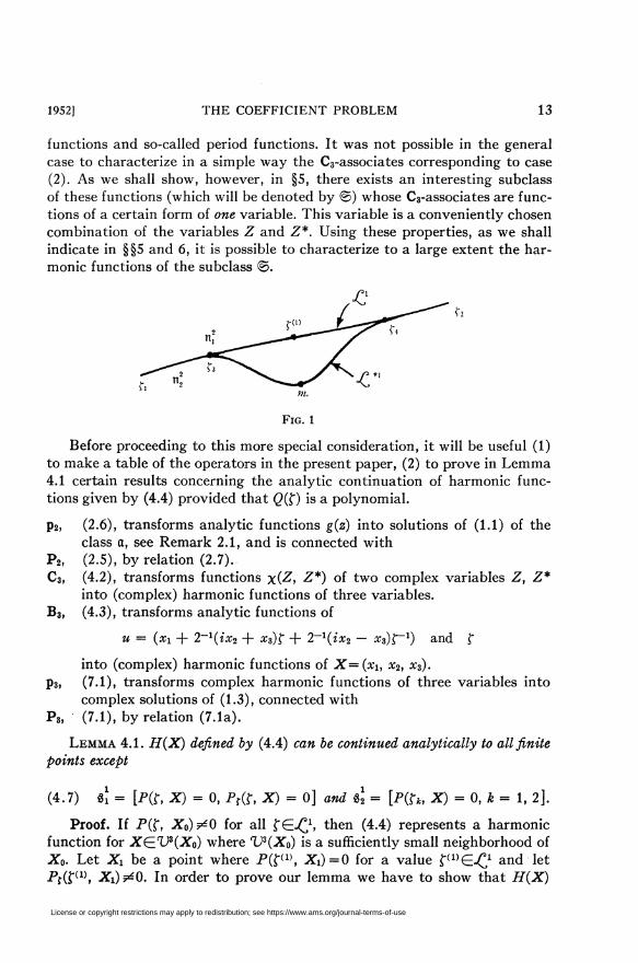
Before proceeding to this more special consideration, it will be useful (1)

to make a table of the operators in the present paper, (2) to prove in Lemma

4.1 certain results concerning the analytic continuation of harmonic func-

tions given by (4.4) provided that (2(f) is a polynomial.

p2, (2.6), transforms analytic functions g(z) into solutions of (1.1) of the

class a, see Remark 2.1, and is connected with

P2, (2.5), by relation (2.7).

C3, (4.2), transforms functions x(Z, Z*) of two complex variables Z, Z*

into (complex) harmonic functions of three variables.

B3, (4.3), transforms analytic functions of

u = (xi + 2~1(ix2 + x3)f + 2~1(ix2 — Xi)^~l) and £

into (complex) harmonic functions of X=(xu x2, x3).

p3, (7.1), transforms complex harmonic functions of three variables into

complex solutions of (1.3), connected with

P3, (7.1), by relation (7.1a).

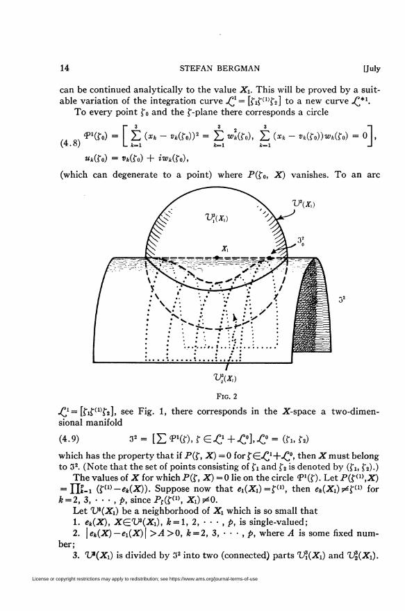
Lemma 4.1. H(X) defined by (4.4) can be continued analytically to all finite

points except

(4.7) «Î = [PÍJ-, X) = 0, Pf(f, X) = 0] and 82 = [P(T*, X) = 0, k = 1, 2].

Proof. If P(f, X0)t¿0 for all fG-C1, then (4.4) represents a harmonic

function for XÇzVz(Xo) where VZ(X0) is a sufficiently small neighborhood of

Xo. Let Xi be a point where P(f(1), Xi)=0 for a value f(1)G.C and let

Pf(f(1), X^Ô. In order to prove our lemma we have to show that H(X)



can be continued analytically to the value X\. This will be proved by a suit-

able variation of the integration curve -£1= [ftru,ft] to a new curve .P/1.

To every point fo and the ftplane there corresponds a circle

,„ « ipl(f») = F ¿ (*» - »*(?»))' = ¿ w*ttà> ¿ (** - »*(fo))wt(ro) - o],(4.8) Lfc-4 *_i fc-i J

«*(fo) = »Jfc(ft) + iwk(Ço),

(which can degenerate to a point) where P(ft, X) vanishes. To an arc

Fig. 2

-C1= [fif(1)fi]i see Fig. 1, there corresponds in the X-space a two-dimen-

sional manifold

(4.9) a2 = [XXrt, r £-0 +CIC = (fi. r»)

which has the property that if P(ft X) =0 for f E°0+-C°>tnen Xmust belong

to 32. (Note that the set of points consisting of ft and ft is denoted by (ft, ft).)

The values of X for which P(ft X) = 0 lie on the circle 'PKft. LetP^^X)

= 11?-! (f(1)-e*(X)). Suppose now that d{Xi) =ft», then ^(XO^ft» for¿fe = 2, 3, • • - , p, since Pf(ft», Xi)^0.

Let V3(Xi) be a neighborhood of X which is so small that

1. ek(X), XEV3(Xi), ¿ = 1, 2, • • • , p, is single-valued;

2. \ek(X) —ei(X)\ >^4>0, k = 2, 3, • • • , p, where A is some fixed num-

ber;

3. V*(Xi) is divided by 32 into two (connected) parts f?(Xi) and 1|(Xi).



Then we have:

v\xo = v\(Xi) + v\(Xx) + 3o, 3o = a2 C\ lf(Xi).

Since ei(X), for XGl^Xi), is single-valued, by the relation

(4.10) r = «i(x),

a one-to-one mapping of points f into segments of lines

ix(f) = ^(f) n tj3(xo

is defined. 32 divides Vz(Xi) into two parts. Since to the points f lying on .£l

correspond segments i'(f) lying on a2,, the values of Ç = ei(X), XEV\(Xi), lie

on one side, say n2; for XE^KXi) on the other side, n!, of the segment ^,

see Fig. 1.

Let ■Pj*1 be a curve which connects fi and f2, and is obtained by replacing

a sufficiently small arc [fsf (1>f4] of jÇ) by a circular arc, [fowîfé], which lies

(except the end points) in rt|.

Then for XCTJ^Xi) we obtain two representations

(4.11a) H(X) = f Q(t)[Ptt, X)]-^d-Ç

(4.11b) =j _«3(f)[P(f, X) ]-"*#.

To the curve .P^*1 there corresponds a segment of a new surface 3*2, which

lies in Vl(Xi)-\-Si but does not contain Xi. Hence there exists a sufficiently

small neighborhood, say V3(Xi), which does not intersect 3*2 and in which

consequently P(f, X), fG-C*1. does not vanish. Hence (4.11b) exists for

XEVs(Xi) and represents the analytic continuation of H(X) to Vz(Xx).

%\ and 82 are (one-dimensional) algebraic curves, and hence they cannot di-

vide the (three-dimensional) X-space into two parts.

This completes the proof of Lemma 4.1. There now arises the question of

how many independent harmonic functions HV(X) are represented by (4.4)

with fixed end points ft, f2.

For every X not belonging to è{, see (4.7), (P(f, X))112 is a function of f

which is determined on a two-sheeted Riemann surface whose branch points

f = ek(X) vary with X

Let jQ be a yôrea curve on the (two-sheeted) Riemann surface of

(P(f, X))1/2 with the end points fi and f2.

If now we vary the point Xi, the right-hand side of (4.4) will yield the

same harmonic function until one of the branch points ek(X\), k = i,2, ■ ■ ■ , p,

intersects „£x. As we indicated before, the relation

(4.12) e*CX>-r, k=l, 2, •••,/>,



for a fixed f defines the circle î>1(f) in the X-space. The surface 32, see (4.9),

will (in general) divide the three-dimensional space into a number of cells,

say ClK-C,1). ^ = 1, 2, - ■ • . The right-hand side of (4.4) will represent in each

of the cells (¡%(j(^) , v=\, 2, ■ ■ ■ , a harmonic function.

On the other hand, in different cells (^(P^), the right-hand side of (4.4)

will represent (in general) different harmonic functions, say Hi(X),

Hi{X), • • • . As indicated before, each function HV{X), v — \, 2, ■ ■ ■ , can be

analytically continued outside the cell (^(P^1), by conveniently varying the

curve(18) jÇf.

According to Lemma 4.1 each HV{X) is defined by analytic continuation

in

-3 1 111

(4.13) *A - g , g = êi + «2,

where zÄ3 = [xj+Xa + x2^ oo ], and g} and §1 were introduced in (4.7).

Let us consider the (three-dimensional) domain zA3 — g1. Its one-dimen-

sional Betti number will in general be different from zero. We now make the

assumption that by a finite number of cuts, ^m, m — i, 2, • • ■ , n, Td2

= 2Zm-i ^5m. we can make the space zA3 — g1 simply-connected. If we move

along a closed curve, D1, starting from the point X0, which curve D1 can be

reduced to a point in zA3 — g1, then obviously upon returning to the values

X0 we shall have the same integration curve ■£' from which we started, and

therefore we shall get for H(X) the initial value H(X<¡).

If, however, our curve cannot be reduced to a point in the space zA3 — g1

(in which case O1 cuts the surface T2), then, in general, upon returning to

the starting point X0, we shall obtain a new curve, say ¿Q, whose end points

are ft and ft, but which cannot be deformed continuously on the Riemann

surface R^Xo) to «Ç1, R(X) being the Riemann surfaces over the ftplane with

branch points e*(Xo), see (4.12). Therefore, the difference between the new

function, say H*(X<¡), and the function FI(X0) from which we started is

2p

(4.14) £ a,(X0)Q,(Xe)v=l

where fív(X0) are so-called period functions and a„(Xo) are integers. The

theory of period functions was developed in [l ] where it was shown that our

functions are defined on R-manifolds with infinitely many sheets and a

method has been discussed, by which, using the theory of hyperelliptic

integrals of one complex variable, we get some information about these func-

tions. In particular, it has been shown that if we introduce certain ^-functions

and their derivatives, the totality of the functions H(X) which one obtains

where Q ranges over the totality of polynomials has in a certain sense a finite

basis: using the above mentioned 0-functions, their derivatives, and finitely

(18) The end points fi and ft of jQ naturally have to be fixed.



many algebro-logarithmic expressions, the fi,(X) can be represented by

finitely many transcendental functions. The functions belonging to this basis

are certain period functions mentioned above.

Thus our method permits us to generate, by evaluating the right-hand

side of (4.4) and varying the neighborhood TJs(Xi), a number of multivalued

harmonic functions. They differ from each other by a combination (4.14) of

period functions.

As indicated before, the curves %\ and %\ are the only possible singularity

lines(19) of functions H,(X).

Lemma 4.2. %\= ][jt-i f(f*) consists of two circles, see (4.7), in the X-space.

Lemma 4.3. Let 2pi be the degree in f o/P(f, X). The curve gj ¿5 (in general)

an algebraic curve of the degree not higher than

(4.15) Spi-3.

Proof. In (4.5) we expressed P(f, X) in polar coordinates p, d, and </>.

In order to determine the discriminant of our equation P(f, X) =0, we write

down the coefficients of f", v = 0, 1, • • • , in

Pi, p, fpf, f p, • • •, f2"i-2Pr, f2"i-2P, r«vipfl(4.16)

P - P(f, X), P( = P^, X).

We obtain a determinant with Ap\ — 1 columns and rows. Every term which

lies in the 2wth row, and «th column, n, is of degree 2, for n = 1, 2, • ■ • , 2pi— 1.

Pj- does not contain p2. Hence the factor p2 does not appear on any other

place except in the above-mentioned terms, and in order to get the highest

degree in p we have to use the product of these terms. Furthermore, we must

take terms of degree one from the next pi columns. Let us now consider the

2¿>ith column. If we take a term of degree one from this column, then we have

taken nothing so far from the first row of the determinant and in all succeed-

ing columns the elements in the first row are 0. Hence, in order to get a non-

vanishing term, we must take in the 2£ith column the term in the first row

which is of degree 0. Hence, we lose 1 degree and the highest possible degree is

2-(2¿! - 1) + l-(pi - 1) + 0 = 5¿i - 3.

5. Harmonic functions of the class @.

Definition 5.1. The subclass of harmonic functions which can be repre-

sented in the form (4.4), (4.5), (4.5a) where 0i(D=0i and </>i(D =<f>i are

constants will be denoted by @.

The harmonic functions H(X)E'B, X=(xi, x2, x¡), are functions of two

variables p and T, see (4.5a).

If we substitute for x\, x2, x3 the values (4.1), the C3-associate of i?G©

(19) They may degenerate in the real X-space.



becomes

(5.1) C, (fl) = I-^^-r—Jri [JR(ft(-25+P(f))]i/2

where

(5.2) S - 2(ZZ*)1/2 cos 0i - i sin AiZe4* - * sin 01Z*e-i*i.

Here 0i and <£i are constants so that (5.2) becomes a function of one variable,

S. Since the C3-associate of every function is uniquely determined, the class

© can be characterized by the fact that C3_1(©) consists of functions (5.1)

of one variable, S, of the form (5.2).

The corresponding harmonic functions become functions of two variables

p and T, of the form (4.4), see also (4.5). (Since di and </>i are constants, T

can be considered as a new independent variable.)

In the following we shall: (I) describe the structure of the singularities of

the functions of the class ©, and (II) show that the coefficients of their series

developments at infinity and at the origin lie in certain subspaces of the

coefficient space.

Let us assume that the coefficient of the highest power of f in P(ft, see

(4.5), is 1. Then for iï£©, see definition 5.1, let

(5.3) ü(f) = Ú(f-4

and let

(5.4) e(r) = E«.r

be a polynomial in f of degree = N.

Definition 5.2. The subclass © of functions (4.4), determined by R and

Q of the above form, for which the degree of Q(ft is =7V will be denoted by

3l(ai, • • ■ ,ap; N).

Lemma 5.1. The only possible singularity curves of the functions H{X)

G3I(öi, • ■ • , flj>; N) are p-\-l circles (which may degenerate) each of which is

the intersection of the plane

(5.5a) xi cos 0i + x2 sin 0i cos <j>i + x3 sin 0i sin 4>i = Re (R(Ç<-k)))

with the sphere

(xi - Re (P(r(fc)) cos 0i)2 + (x2 - Re (Ä(f <*>)) sin 0X cos <¿>i)2 + (*«(5.5b)

- Re CR(f<») sin 0i sin <*>i)2 = (Im P(f<*>))2;

and the straight line consisting of the rays



(5.5c) <t> = 4>i, 0 = 0i and <f> = <pi + t, 0 = — 0i.

Here ftw, k = l, 2, • • • , p-l, are the (p-l) solutions of P'(ft=0 and

r(î,,=ri>f(p+l,=r2.

Proof. The equations P(ft X) =0, see (4.5), and Pr(ft X) =0 in this case

assume the form

(5.6) P2 + Rtt)[-2Tp+R(ï)] = 0,

7" = cos 6 cos öi + sin 6 sin 0i cos (<f> — <£i),

(5.7) P'(f)[-2rP+2P(f)] =0,

respectively. There are two possible types of solutions of (5.7):

(1) P'(ft=0: We obtain p — 1 (generally) distinct values for ft say

£" = ft"), k = 1, 2, • • • , p — 1. Substituting these values into (5.6) gives p — 1

circles. Adding two circles corresponding to tdie end points ft and ft, we ob-

tain p + 1 circles.

(2) R(Ç)=pT: substituting this into (5.6), we obtain p»(l-rs)=0. P2

is always less than or equal to one, and may equal one only if <¡>=<pi, 6—0i,

and <p=<pi-\-ir, d= — 0X. All other possibilities lead to a different representa-

tion of the same line. The origin lies also on this line so that the case p = 0 is

already included. This proves our lemma.

Before proceeding further, it will be of interest to discuss in detail the

simplest example, namely where P(ft =A-\-BÇ is of the first degree. In this

case, we can carry out the integration and we obtain

(5.8) H(X) = ^(-1)'FK,«=i

(5.8a) FK = log [C, + (CU + D)m], C. = BÇ. + A + pT, D = p\l - t\

We shall determine the singularities of FK in the real (finite) space,

x2+3'2+z2< oo. The only singular manifolds which can possibly occur cor-

respond to the following four possibilities:

(5.9.1) C, = 0, D^Q, (5.9.2) CK ̂ 0, D = 0,

(5.9.3) C, = 0, D = 0, (5.9.4) c] + D = 0, CK ¿¿ 0.

In the first case, the function is regular on the manifold (5.9.1), since the

function FK has the development 2_1 log P/ + C+ • • • . It can be singular

only for D = 0, i.e., in the case (5.9.3).

The expression in brackets on the right-hand side of (5.8a) is two-valued.

In the case (5.9.2), we obtain in the second sheet a logarithmic branch line for

Z> = 0, i.e., for [<p=<f>i, d=6i] and [<p=cpi+T,6= —0i], where we have a branch-

line of infinite order.



The third case, (5.9.3), can occur only if P(f«) is real, and we obtain an

isolated point 6 = &i, <p=(pi, p= — P(f«). (This point lies on the line D = 0.)

The case (5.9.4) leadg to the circle P(f«, X) =0 on which the function is con-

tinuous but on which the derivatives are infinite. We obtain, for instance,

dH TP(f.) + 2p - pT2-=-h reg. terms.dp CK(Cl + Z?)1'2

In the case where P(f) is of a higher degree, the functions can be represented

in closed form using hyperelliptic integrals, and a similar discussion can be

carried out.

Remark 5.1. If H(X)(E<S>, then the location of its singularities and the

value of P(0) determine the quantities ai, • ■ • , av in (5.3).

We proceed now to the problem II.

Outside of a sufficiently large sphere, we can develop a function (4.4) of

the class © in the form of an infinite series of spherical harmonics

Z ßnP~{n+l) |Pn(cOS 0)P„(COS «,)n-0 L

" (» — V) ! , „ "I+ 2 2Li -P„(cos 0)Pn(cos öi) (cos v<j> cos vcpi + sin v4> sin v<pi) .

„_i (n + v)\ J

(5.10)

Definition 5.3. An expression depending only on the aj,j = l, 2, ■ ■ ■ , p,

and N will be said, for the sake of brevity, to belong to a^.

Theorem 5.1. A necessary condition that the series (5.10), where 0i and fa

are arbitrary, real constants, represent a functions element (at infinity) of a

function of class 3I(öi, • • • , av; N), see Definition 5.2, is that for every integer

R^Rm(p, N)=6(N+l)(N+2)(N+3)p + 7, there exist a set of numbers

{A%*}, 5 = 1, 2, • • • , sB; R=RX, Rx+l, • • • ; A%>mA<**(ait N)eaN,

so that the relations

(5.11) X ¿,,,lT ft&0r = 0, s = 1,2, ■■■ ,sR,R = Rx, R„ + l,- ■ ■

hold(20). Here A%% s = l, 2, • • • , sR, for p+<r+r=R are not all zero(21).

Proof. Since (1 -2p-1TR(t)+p~2R2(^))-1'2, with P = cos a and RQ)-1,

is the generating function of the spherical harmonics, we obtain that ßn in

(5.10) are given by

(20) A'££T are independent of «x, X = l, 2, ■ • • , N, as well as of fi and f2- Explicit formulas

for Af^T, BpRftT (see Theorem 6.1), as well as for some other quantities considered in the fol-

lowing, can be obtained by straightforward computation. Since they are quite involved, they

have been omitted from the present publication. They can be found in the Technical Report

No. 32 of the series Studies in Partial Differential Equations, Cambridge, 1951.

(21) This implies that we have infinitely many distinct relations (5.11).



(5.12) ft,= f 'QÜ)[R(t)M,J fi

where Q and R are polynomials, see (5.3) and (5.4), so that

n(P-l)+N N

(5.13) ft = Z T,F(j, \ «H[(ft - «i)"+i+1 - (ft - ßi)"+i+1],)=o x=.o

where F(j, X, n) are certain functions of the a¡. (See footnote 20.) Our aim

is to obtain relations among the /3n's which depend only on a¡, but are inde-

pendent of ft, ft, as well as the coefficients e\ of Q. For this purpose, we multi-

ply three ß„'s by each other, and get relations of the form

N Xi X2 [(ÄH-3(iV+l))/2] a

ftftrft = XI X) X H 11 S(oí, ß; Xi, X2, X3; p, a, t),_ ... Xl=0 X2=0 X3=0 o-l 0=0

(5.14) . .X {(ft - <zi)*(ft - fli)" - (ft - ßi)"(ft - aO^íx^íXs,

where 5Gajy. In the following, we shall consider the expressions

(5.14a) {(ft - fli)«(ft - aiY - (ft - ai)«(ft - atf}exîx,

as variables which eventually have to be eliminated from the equations (5.14).

To prove Theorem 5.1, we need a number of lemmas which are for the most

part evident.

Lemma 5.2. The number of non-negative integers satisfying the inequalities

0 ^ Xi á X, | X, g JV

is(N+l)(N+2)(N+3)/6.

Lemma 5.3. The number of distinct ways of writing an integer R>2 as a

sum of three positive integers is larger than P2/6.

Lemma 5.4. // P>(A7'+l)(A7'-)-2)(iV+3)2Í>, then the number of variables

(5.14a) for which a-\-ß appearing as exponents in the right-hand side of (5.14)

assumes its maximum value Rp + 3(N-\-l) is less than the number of equations

(5.14) for which p + <t+t=R.

Proof. By Lemma 5.3, the number of equations is larger than P2/6. The

number of variables is

(N + 1)(N + 2)(N + 3) ^ | Rp + 3(N + 1)\(5.15) 6 Y+ 2 |.

If R satisfies the conditions of Lemma 5.4, it is obvious that P2/6 is larger

than (5.15).

We now estimate the number of triples (p, cr, r) such that p+ff+r^P



and O^p^ít^t.

The number of distinct ways of writing an integer M as the sum of two

positive integers is ^ [Af/2](22). Hence the number of distinct ways of writing

all positive integers i£ M as a sum of two positive integers is larger or equal to

FMI FM - 11 VM -21 V11 YM12(5.16) [_]+[_] + [_] + . ••+[T]i[T].

We now proceed to the determination of the number of distinct ways of

writing all integers ^ M as the sum of three positive integers. Suppose that

the smallest of these three integers is K. Then the number of triples whose

smallest member is K is the same as the number of distinct pairs adding up

to M—K where each member of these pairs must be larger or equal to K.

This number is by (5.16) larger than

(5.17) [(M - 3K)/2]2.

If K varies from 1 to [M/3] (since K is the smallest of the triple, K ^ [Af/3])

we obtain all possible triples. It remains to determine a lower bound for

(Ml*)

(5.18) £ [(M - 3K)/2]2.JC-0

We shall show that for M ^36

(5.19) (M - 7)3/36

is such a lower bound. If we write the sequence [(M — 3K)/2]2, K

= 0, 1, 2, • • • , then we obtain a consecutive series of squares decreasing

from [M/2]2 to l2, with every third term missing. The worst possibility is if

the numbers [(M-2-6k)/2]2, k = 0, 1, • • • , [(Af-9)/6]2, are missing. We

obtain therefore that (5.18) is greater than or equal to

[Ml 2] [(M-2)/6] 1

£rc2-9 £ n2 = — {[M/2]([M/2]+l)(2[M/2] + l)n=l n-1 6

(5.20) - 9[(M - 2)/6]([(M - 2)/6] + 1)(2[(M - 2)/6] + 1)}

1 11 1 ) 1è — \~ (M - 3)3-(M + 3)»> ^ — (if - 7)3, for M ^ 36.

6 14 12 j " 36

Thus, if p, cr, T covers all distinct possibilities so that p + ff+r = P, then the

number of equations is larger than (R — 7)3/36. On the other hand, adding

expressions (5.15) for R = l, • • • , R = R(23), we see that the number of dis-

(22) [5] denotes the largest integer which is smaller or equal to S.

(23) In order to avoid subscripts we use the same symbol R both as a summation index

and as the upper limit.



tinct variables (5.14a) in these equations is

(N+ 1)(N + 2)(N + 3)(5.21)--R(Rp+ 10 +6N + p).

24

A simple calculation shows that under the hypothesis of Theorem 5.1,

1 (N + l)(N + 2)(N + 3)(5.22) — (P-7)3>---R(Rp+ 10 +6N + p).

36 24

Indeed: R<2(R-7) if P>14, and Rp + 10+6N+p<2(Rp-7p) if P>25+ 6N. In addition to that, according to (5.20), P^36. It is now clear that

iî R>6(N+l)(N+2)(N+3)p + 7, then (5.22) is satisfied, and this condition

implies the three previous ones.

We wish to show that if we have m equations

n

(5.23) HA^X,, = Ly, v = 1, • • • , m,

in which n variables X„ occur, m>n, then, necessarily, we obtain at least

(rn — n) distinct relations among the AVß and Lv. They are linear in L, and

lead to (5.11). If we write Xn+i = l, the system (5.23) becomes

n

(5.24) £ AV,X, - LrXn+i = 0, v = 1, 2, • • • , m.

Since m^n + 1 and since we know that not all X„, ß = l, ■ ■ • , n + 1, are

identically equal to zero, the determinant of any system of (n + 1) equations

(5.24) equals zero. This yields at least one relation between the L, and the

A,ß. Thus, we get at least m — n independent relations.

The system of relations (5.14) is of the type (5.23). Here, L, are theftAft's,

(5.25) X, = [(ft - ajHft - aiY - (ft - ffl)"(ft - aiY}^^,,

and the Ay» are the coefficients S(a, ß; Xi, X2, X3; p, <r, r). The latter belong to

the class ajv, introduced on p. 20. If R is increased in the equations (5.14),

new AV)l and Lv appear. By Lemma 5.4, these new Avil's and L,'s will actually

occur in the determinant of (5.24) which we obtain for every new R. Thus at

each step we obtain a new relation involving some Ayf¡'s or Ly's, which did

not appear previously. This proves Theorem 5.1.

Remark 5.2. The ^4**' for a fixed R are, according to our proof, certain

subdeterminants of the matrix of coefficients

(5.26) [S(a, ß;\i, X«, X3;p, <r, r)], p + <r + r ^ R.

A detailed description of these expressions is given in the appendix.

Example, p = 1, N = 0, P(f ) = (f - a).



In this case, the harmonic function under consideration is

•r. #

(5.27) H(X)= fri [p2+(f-ö)2-2p(t-a)(cos9cos9i+sinösinö1cos(0i-</)))]1/2

Then the coefficients /3„ of the development (5.10) at infinity satisfy an

infinite number of relations (5.11), of which the first two are:

fofo - 3ß,ßxß2 + 2ß\ = 0,

Sß\ßi - 8/îofrft - 9ß0ß2 + 12/3& = 0.

6. The development of a function of the class © at the origin, and its

properties. In a sufficiently small neighborhood of the origin, we can develop

the function (4.4) in a series of spherical harmonics

mx> - ffs Q(m

h (P(r,-y))i/2

Q(t)d

u _«, (P(f))'

/■ {■> " 0(OdfS ,n/\V4.,Pn[P»(C0S 9)P«(C0S ̂

t, n=o (P(r))n+1

rf2 a e(f)¿f= y. -p"P„(cos 6 cos öi + sin 0 sin 9i cos (<£i — 4>))

Jr, „=o (P(r))n+1(6.1)

't. n=o (R(nr" (* - 1») I „

+ 2 2^ -Pn(cos 0)P„(cos ôi)(cos c0 cos f0i„=i (w + v)l

+ sin y<£ sin vfa) ].

(See [13, vol. 1, p. 400, (44)].)Thus the coefficient of the term p"P„ (cos 6) is

r12 Q(û<ttTÂÍcob*), . Y-+1 = Jn (i?(r))„+1'

while the coefficient of pnP"„ (cos 9) cos f<£ is

(» — !»)! „27n+i-P„(cos 0i) cos vcpi.

(» + v) !

Theorem 6.1. ^4 necessary condition that the series

(6.2) X) P" <TnP„(cos 0) + ¿ pI(cos 0) [t»Í cos v<p + r«; sin v<t>] >n=0 V v=l /

represent a series development at the origin of a function of the class

2I(öi, • • • , ap; N) is that there exist constants &i and fa, \di\ ^x/2, \fa\ ¡Sir,

and a series of numbers y „, »«1,2, • • -, such that



(6.3a) rn = 7„+iPn(cos 0i),(1) V

(6.3b) (n + v)Wnv = 2yn+l(n — v)\Pn(cos 0i) cos v<pi,(2) v

(6.3c) (n + v)\rnv = 2yn+i(n — v)lP„(cos 0i) sin v<pi,

and that for every integer R^R0(p, N)=3(N+l)p[2(N+2)(N+3)p2+l] + 7,

there exists a series of numbers P^£a¿v (see Definition 5.3 and footnote 20)

so that

(6.4) 2^ BP,',r yp-Yelr = 0, s = 1, 2, ■ ■ ■ , su; R = Ro, R0 + 1, ■ ■ ■ .p+n+räR

Here Bpf;% s = l, 2, ■ ■ ■ , sx, for p + cr+r =R are not all zero(2i).

Proof. The proof is in principle similar to that of Theorem 5.1, but some

modifications have to be discussed. In this case,

C" 0(0 „ C" 0(f)«

n (f - ««)n«=1

The variables Yn which we shall eliminate are in this case

,. « F" - foi - «¿)-"(ft - a,)H» - (ft - fli)—(ft - aj)-e]e^(h,(6.6)

a ^ ft 0 ^ Xi ^ X2 ̂ X3 ̂ iV.

The following three additional complications arise in this case.

(1) Since, say, (ft —fly)" now appear in the denominator we can not ex-

press it in finitely many terms (ft — ßi)-"' of the same form. Hence, a much

larger number of variables F„ have to be eliminated.

(2) In order to express the integrand of y„ in terms of the variables F„

we have to use partial fractions. Furthermore, after we multiply three y„

together, we again have used partial fractions to express 7P7<,7r in terms of

F„. This situation makes the coefficients of the Yn very much more compli-

cated.

(3) After we express the integrand of yn in partial fractions and integrate,

we obtain p(N+l) distinct logarithmic terms. Using the first p(N+l)

formulas for yn we can represent these logarithmic expressions in terms of

7„, w = l, 2, • • • , p(N+l). The logarithmic terms in the formulas for

yp, p>p(N+l), must be replaced by these terms, before we form the expres-

sions 7P7„7T.

As a consequence of these three complicating factors, the coefficients

B^l in the relations (6.4) will be much more involved and R<¡(N, p) will

be very much larger than RM(N, p).

In order to evaluate (6.5), we separate the integrand in partial fractions,

(24) This implies that we have infinitely many distinct relations (6.4).



and we obtain (26)

¿v p n /• ¡

F=0 IC=1 J—1 J f 1

. (n)

- »f(f - ««)'

JV p n ,4 "' c

(6.7) -EH ^^ [fo - a«)-'"« - (ft - «,)-^j

, ä a . <-) , a* - ««)+ 2^ Z, AK,!,rtr log- •

„=0 «=1 (fl — Ö«)

Herede«».The expressions yn all contain the same (N-\-l)p logarithmic terms.

Remark. Here we assume that the determinant

I -I*1' Am Am Am Am A(1) Am A{1)

Auo " • • Apio Am ■ • • Apu Am " • " Apti ■ • • Aim ' • ' Apin.(2) .(2) (2) .(2) (2) .(2) .(2) (2)

Ano " ' " Apia Am • • • Apa Am • • • Apu • ■ • Aim " " • ApiN

.(Np+p) .(Np+p) .(Np+p) .(Np+p) .(Np+p) .(Np+p) .(Np+p) .(Np+p)Ano ' ' ' Apio Am • • • Apii Am • • ' Api2 • • • Any • • • Apin

does not vanish. Should this not be the case, then we have to use more ex-

pressions(6.7).

If we use the (N+l)p first relations (6.7) the e„ log [(f2 —a«)/(fi-a«)]

can be expressed in terms of y„, n^(N-\-l)p, and rational terms, i.e., we

have

(f2 - aK) »r+i),

(6.8) (fl_<g m=1

(N+l)p N p n

n=2 r=0 «=1 ;'=2

where rro and B(")ir belong to a^. (See Definition 5.3.)

Replacing for every n>(N-\-l)p the logarithmic terms in (6.7) by (6.8),

we obtain that a certain linear combination

(tr+Dp (n)

(6.9) Bn = 7„ — Z Am ym; Am G aw,7»=1

is a rational expression,

p » if r¡, w~i

(6.10) «. = E Z E ' . [(fi - *)*-' - (fi - a.)1-'] *,1=1 j_2 i—O Lk, jj

» = (N + i)p + 1, (2V + 1)¿ + 2,. • • ;

(26) Explicit formulas for the A™¡lP as well as for all subsequent expressions may be found

in the article mentioned in footnote 20.



p, n\

J.

being some functions belonging to a#.

By multiplying two 5„ we obtain, as we shall prove,

JV ci r p p+o— 2

5p5«r = 12 12 efiti'i] 12 12 G(k, v, pi, p2; P, <rCI—0 es— 0 V «—1 r=l

X [(ft - aK)- + (ft - aK)~'}

(6.11) * * ' ' Tpi, pi |-P2, o-l- 12 12 12 12 \. .. . ((ft-«ii)-,i+1(ft-«i8)-,2+1

il—1 i2=l Jl-2 j2=2 LU, JlJ Ll2, JiJ

+ (ft - «i2)-/2+1(ft - aO-A+4

where G(k, v, pu p2; p, cr)£ajv.

Proof of (6.11). By multiplying two expressions of the form (6.10) for

n =p and n = <r, we obtain on the right-hand side sums of the following types

of expressions:

1. (ft — ai!)-il(ft — ai2)~'2, ii ^¡2, and analogous expressions in ft (in-

stead of ft). Applying the method of partial fractions to these terms, we ob-

tain expressions appearing in the first sum in the bracket in (6.11).

2. If ii = i2 the above expression becomes (ft —oí1)-('1+í,) from which we

obtain again expressions of the same form.

3. Mixed terms of the form (ft —a^îft —úh,)-'2 which cannot be sepa-

rated in any way are collected in the last sum of (6.11).

Multiplying three ô„ together, we obtain

JV m M2

(6.12) hfiehr = 2Z 12 12 «crWcaCSlC"!. M2, Pi) + S2(ßl, Pi, Pi))Cl—0 C2—0 C3—0

where

V p+ff+T— 3

Si(pi, Pi, Pi) = 12 12 H(s, X; pi, p2, p3; P, cr, r) [(ft - «.)"" - (ft - «»)"''],8=1 ,,= 1

p P ff+T—2 min(r—l,p+(7+T—3—c)

Si(pi, P2, Pi) = 12 12 12 12 T(¡i, s,\, t; pi, pi, p3; p, o-, t)8=1 Í-1 C-l X=l

X [(ft - o.)-"(ft - a,)-x - (ft - ff„)-"(ft - at)-*],

and the H's and the P'sGajy. (6.12) is obtained by repeating the previous

arguments.

The proof of the relations (6.4) now proceeds analogously to that of

(5.11).If we compare the variables X„ (introduced in (5.25)) with the F„ (intro-



duced in (6.6)) we see that they are exactly of the same form, with the only

difference that while in (6.6) expressions of the type

[(f2 - <n)-«(fi - Of)-" - (fi - ai)-«(f2 - ffi)-"]««««^,

i = 1, 2, • • ■ ,p;j = 1, 2, • • • , p,

appear, in (5.25) only expressions with i = l, _/=l do appear. Therefore, in

the case of the Yn we have p2 as many variables as in the case of the Xn.

Thus according to (5.21) the number of the variables is

(6.13) ((N+ 1)(N + 2)(N + 3)/24) R(Rp + 10 + 6N + p)p\

In order to determine the number of equations, we recall the considerations

on p. 23 of §5. We have, however, to take into account that p, a, t, in ad-

dition to the restriction p+cr+r^P, must each be larger than (N-\-l)p,

since the first (N-\-l)p relations are used to eliminate the logarithmic terms.

Hence, the number of equations will be larger than

(6.14) [R- 3(N+ l)p - 7]3/36.

In an analogy to the considerations on p. 23, we find that (6.14) is

larger than (6.13) if

(6.15) R ^ Ro(P,N) = 3(N+ l)p[2(N + 2)(N + 3)p2 + l] + 7.

Repeating analogous considerations as in §5, we obtain that the ôpô„ôT's

satisfy relations of the form (6.4). But since, according to (6.9), the 5n's

are linear combinations of the Y„'s, the relation (6.4) follows.

7. Solutions \¡i(X) of (1.3) of the class © and relations among their

coefficients. In (5.26) of [6] (see also (4.3) of [8]) we have introduced the

operators P3 and p3 transforming harmonic functions into solutions of (1.3) (26)

(7.1a) vKX) = P3(P) = J Ü(p, r)H(X(l - r2))dr

(7.1b) = p,(G) = G(X) + ¿£(»»M f (1 - <r2)"â2G(<r2X)da,71=1 J 0

where £2(p, t) and P(n)(p2) are entire functions of p2. See (4.3) and (4.4) of

[8]-Here G(X) and LI(X) are connected by the relations

(7.2a) G(X) = f P-^ííXXa - T))dT,J o

(26) In [ó] we used the letter H instead of Ü, employing Ü in the more general case of

equation T(^) =X>2t+A(pi) X V^ + C(p2)^ = 0. If ¿=0, C=F, see (2.2) of [6], we obtain

the case considered in the present paper. Our results can easily be extended to the case of an

equation T(\p) =0 where A and C are entire functions of p2= 2~Ll-i **■



see (4.8) of [8], and

H(X) m H(p,e,<p) = 2T-V'2d[pi>2 j G(pt2,6,<p)(l - t*)-ll*dt]/dp,

G(X) = G(p, 0, <¡>).

Proof of (7.2b). Let G and H be the p3-associate and the P3-associate, re-

spectively, of the same solution \j/. If we write

X

G(X) m G(p, 6,4>) = 12 PvQp(ß, <t>)p=0

and H(X) = H(p, B, <p) = 12P=0 Pp1p(^< 4>), where Qp(0, <p) and qp(9, <p) are func-

tions of 0 and <p, \d\ ís.ir/2, \<t>\ ̂tt, then according to (4.8) of [8]

= 7¿fí + 7)ppep(ö,*) f ¿mi-*2)-i/2^,2 p_o \ 2 / Jo

from which (7.2b) follows.

As we have shown in Lemma 4.2, p. 502, of [8]

... 2 2 1/2 2 2 1/2(7.3a) vv(x2 + x3) , x2, x3) = G(i(x2 + x3) , x2, x3),

i.e.,

(7.3b) cr'w = crWw),see (4.15(27) of [6].

It follows from (7.1) that ^(X) is regular at every point X where H is

regular.

Definition 7.1. Extending the definition 5.1 we shall say that solutions

of (1.3) whose C3-associates are of the form (5.1) belong to the class ©.

Definition 7.2. If G(X) =P0T-^H(X(l-T))dTGn(ai, ■ ■ ■ , ap; N),then (extending the definition 5.2) i// = P3(iP; =p3(G) will be said to belong to

the subclass §I(ai, ■ • • , ap; TV); ipE$.(ai, ■ ■ ■ , ap; N).

From our previous statements follows the

Lemma 7.1. The only (possible) singularities in the finite X-space of a

solution i/y(X)£2l(cii, • • • , ap; N) of (1.3) are the circles (5.5a), (5.5b), and

the straight line (5.5c).

Remark 7.1. Thus as in the two-dimensional case the location of the

(27) In (4.15) of [8] b3~' should be replaced by p»-1. It should be stressed that, on the left-

hand side of (7.2b), C3 refers to the operator transforming x{Z, Z*) into solutions of (1.3),

while on the right-hand side it refers to the operator transforming x{Z, Z*) into harmonic

functions.



singularities is completely independent of the coefficient F of (1.3).

Lemma 7.2. Every real solution of (1.3) which is regular at the origin 0

can be developed in a sufficiently small neighborhood of 0 in a series

(7.4) vHX) - fa 0,4>) = i i Pn+' ± BÍ-'p!:1 (cos 8)eim*,n=0 v=Q m=~n

<„,„) („,„)

J>« = -D-m •

PAe representation (7.4) ¿s unique(2i).

Proof. Let

(7.5)tf(X) - P(P, 0, 0) = ¿ p" [^"^„(cos 0) + ¿ P^'pL"" (cos 0)«'"*],

rt=0 I— m=—n J

R(n) - RM

Since according to (3.10), p. 425 of [6],

(7.6) o(Plr) = l + ¿r¥"(p!),>—i

it follows from (7.1) that

t(X) = ftp, 0, 0) = f |"l + P2Z r2^0(p2)p-2l

(7.7) m J-lL -1 n J

X r ¿ p»(l - r2)"(^„oP„(cos 0) + ¿ P^pIT' (cos 0)eim*)l ¿tL n=0 \ in=—n / J

where p~-b{n)(p2) are according to (3.9), p. 425, of [6] entire functions of p2.

Both series (7.5) and (7.6) converge uniformly and absolutely in every

sufficiently small sphere around the origin (see Lemma 3.2 of [6]); hence,

interchanging of the order of summation and integration is permissible. Thus

HX) = T,P"( f (1 - T2)Hr\An0Pn(cos6) + ¿P^pIT'(cos 0)eim*ln=0 \ J — 1 L 77>=—n J

+ P2¿P-2¿C"V) f (1 -T2)"T2'dT \An0Pn(cOSd)

m=—n «J/

(28) It should be stressed that in Theorem 4.1 of [ó] we proved a similar result. We con-

sidered there however a sphere of a given radius, while in the present paper we consider only a

sufficiently small neighborhood of the origin.



If we write

InoJ (1-2n (n,0)

t ) a-T = ß0 ,

bI' J (1 - t) dr = Bm ',

we obtain the formula (7.4) since p~2b<-") (p2) are entire functions of p2.

Theorem 7.1. The subsequence {B^0} of the coefficients of the series de-

velopment (7.4) at the origin of a function \p(X)^%(ai, • ■ ■ , ap; N) satisfies

the following conditions. There exist two real numbers <f>i and di, |<pi| ^-ir,

10i| Hkir/2, and an infinite sequence of numbers yn which for R^R0(p, N)

satisfy the relation (6.4) and such that

(7.8a) B*' = yn+iPn(cos6i),

(7.8b) (n + v)!(/jln'0) + /¿n;0)) = 47„+i(« - v)!Pl(cos 0x) cos vfa,

(7.8c) -i(n + v)l(Bn'0) - B^°) = 4yn+i(n - v)lP*n(cos 0i) sin v<Pi.

Remark 7.2. In analogy to the two-dimensional case the conditions formu-

lated in the Theorem 7.1 are independent of the coefficient F of the equation

(1.3).Proof. According to Lemma 7.2 and the representation (7.7), a solution

\p of the equation (1.3) is completely determined by the subsequence {P^'0'}.

By (7.3a), if ^G9I(ai, ■ ■ ■ , ap; N), p^1^) must satisfy the conditions (6.3a),

(6.3b), (6.3c). This yields our theorem.

In analogy to the second part of the Theorem 2.2 we obtain

Theorem 7.2. If ^G2i(ai, • • ■ , ap; N), it can be represented in the form

t(X) = !(7\ p)

(7.9) d[pV2f*mj(B'+^,gi,giy]= — 0(p, r) -Í!-dr

2ir J T=_i dp

where J(s, g2, gz) is the inverse of the Weierstrass ^-function and T is given by

(4.5a). Here

(7.10a) gi = - IBB' + 3C2, (7.10b) gs = 2BCB' -AB'2- C3

and

A = - p2(l - r2)2, B = [2P(ft(l - r2)pT + p2(l - r2)2]/4,

C = - [7?2(ft + 2P(ft(l - r2)Pr]/6, B' = P2(f)/4.

Proof. It follows from (7.1a) and (7.2b) that ^ can be represented in the



form

HX) - — f a(p, r)p^-

(7.12)-1/'<7T JT-1

X {¿Tp1/2 f G(p/2(1 - r2),0, 0)(1 - t2)-^2dt\ / dp\ dr.

Since ^G2l(ai, ■ ■ ■ , ap; N) and C-"3^) = C_3(G), according to the Definition

5.2, (4.4) and (4.5),

r> Q(m

dl

(7.13) G(p,e,<t>) = (Jh [p2 + P2(f) - 2P(f)PP]"2

Thus in this case

f [C7(p^(l -r2),0, 0)](1 -*2)-^J o

(7.14) = r1 r_^_•Wn Í [<V(1 - r2)2 - 2¿2P(f)P(l - t2)T + P2(f)](l - i2)}1'2

i rl2 r f1 ¿íc "i(7.14a) =— Q(f) -U-

2 Jfl L J.=o 04*4 + 4P«3 + 6CV + 4P'*)1'2J

where A, B, C, B' are functions of p, T, r, f introduced in (7.11).

By the transformation s(x) =B'x~1-\-C/2, see I, p. 13 and III, p. 14 of

[20], the interior integral in (7.14a) goes into

CB-+cn ds / C \(7-15) - 771-7i7¡ = / (B' + ^>S2<S* ).

J» (4s3 - g2s - gs)1'2 \ 2 /

see p. 229 of [20].

Substituting this expression for the interior integral in (7.14a) and re-

placing the interior integral in (7.12) by the new expression we obtain

(7.9).8. Concluding remarks. As we stressed in the introduction, the interest

of our considerations is not merely in the isolated results formulated in the

paper, but rather in establishing methods of exploiting the laws which con-

nect different classes of functions obtained with the help of mappings by

integral operators of the first kind. In this connection it is of interest to use

also other integral operators. In particular, as has been shown in [5], the

representation of harmonic functions with the help of the fundamental solu-

tion can be employed to define a mapping by an integral operator. Using the

fundamental solution of

(8.1) A^ + F(xu Xi, x3)$ = 0,



see [l4b], a mapping analogous to (4.4) of polynomials Q into solutions of

equation (8.1) can be introduced. This mapping permits us to extend a large

part of the results of [5] to the case of differential equations(29) (8.1).

A further type of integral operator which is valuable for the study of cer-

tain types of differential equations (8.1) is that for which the generating

function E can be represented in the form

(8.2) E = P(X, t) log Q(X, t), X = (xi, Xi, x3),

where P and Q are polynomials in t. (Procedures used in [2, §3] can be re-

peated in the three-dimensional case to a large extent.)

In some instances singularities of differential equations in three variables

can be obtained by reducing them by a convenient substitution to equations

in two variables, e.g., the substitution ^(x, y, z)=cos pz\p(x, y) reduces

***+*w+*„ = P(x, y)V totxx+4>yy=(v2+P(x, y)W.

The relations between the coefficients of the function element of \p and

the property of the solution \p obtained by the use of integral operators dif-

ferent from those of the first kind in most instances depend upon the coeffi-

cient F so that we are led by these operators to new types of theorems.

It should be mentioned also that similar to our results, relations between

the subsequence \amv}, m=0, 1, 2, • • • ; v>0, of the coefficients of the func-

tion element \p = 12amn zmz*n of the solution \f/ and its properties can be estab-

lished, see [15].

The functions considered in the present paper represent the simplest

class of solutions of (1.1) for which representations in terms of classical func-

tions can be obtained. (See Theorem 2.2.) It is known (see [14, §§14-16],

[14a, §§14, 16]) that if a function g is a solution of an ordinary linear dif-

ferential equation

(8.3) ¿ Pn-,(z)gw = 0, fw = d'g/dz',?=0

where Pf,(z) are algebraic functions of z satisfying certain conditions, the

integrals Jl(z — Dn_1g(D^r and P_ig(z(l—t2))dt/t2 can be represented by

automorphic 0-functions and related functions. Using these results, one ob-

tains representations analogous to those indicated in Theorem 2.2 for solu-

tions of (1.1) whose C-associates (see p. 2) satisfy equations of type (8.3).

Similar theorems can be obtained also in the three-dimensional case for

certain solutions of (1.3). See also [l, §5], in particular p. 551.

Thus one sees that the method of integral operators opens various and

fruitful possibilities in such a comparatively little explored field as the theory

of multivalued solutions of linear partial differential equations.

(29) It should be mentioned that the method of the integral operator of the first kind can

be extended to the general equation (8.1) as will be shown in another place. Since some addi-

tional complications arise in this connection we do not discuss this case in the present paper.


34 STEFAN BERGMAN

Bibliography

1. Stefan Bergman, Zur Theorie der algebraischen Potentialfunktionen des drei-dimensionalen

Raumes, Math. Ann. vol. 99 (1928) pp. 629-659, and vol. 101 (1929) pp. 534-558.2. -, Zur Theorie der Funktionen, die eine lineare partielle Differentialgleichung

befriedigen, Rec. Math. (Mat. Sbornik) N.S. vol. 2 (1937) pp. 1169-1198.3. -, Linear operators in the theory of partial differential equations, Trans. Amer. Math.

Soc. vol. 53 (1943) pp. 130-155.4. -, Certain classes of analytic functions of two real variables and their properties,

Trans. Amer. Math. Soc. vol. 57 (1945) pp. 299-331.5. -, A class of harmonic functions in three variables and their properties, Trans.

Amer. Math. Soc. vol. 59 (1946) pp. 216-247.6. -, Classes of solutions of linear partial differential equations in three variables, Duke

Math. J. vol. 13 (1946) pp. 419-458.7. -, Operator methods in the theory of compressible fluids, Proceedings of Symposia in

Applied Mathematics, American Mathematical Society, vol. 1, 1949, pp. 19-40.

8. -, On solutions with algebraic cltaracter of linear partial differential equations, Trans.

Amer. Math. Soc. vol. 68 (1950) pp. 461-507.9. -, On solutions of linear partial differential equations of mixed type, Amer. J. Math.

vol. 74 (1952) pp. 444-474.10. L. Bieberbach, Lehrbuch der Funktionentheorie, vol. 2, Leipzig, Berlin, 1931.

11. M. M. E. Eichler, On the differential equation uzz-\-uyy-{-N(x)u — 0, Trans. Amer.

Math. Soc. vol. 65 (1949) pp. 259-278.12. -, Analytic functions in three-dimensional Riemannian spaces, Duke Math. J. vol.

16 (1949) pp. 339-349.13. P. Frank and R. v. Mises, Die Differential- und Integralgleichungen, 2d ed., vol. 1, 1943.

14. R. Fricke, Automorphe Funktionen mit Einschluss der elliptischen Modulfunktionen,

Encyklopädie der Mathematischen Wissenschaften II B. 4, Leipzig, 1921.

14a. E. Hilb, Lineare Differentialgleichungen im komplexen Gebiet, Encyklopädie der

Mathematischen Wissenschaften II B. 5, Leipzig, 1921.

14b. E. Holmgren, Über die Existenz der Grundlösung bei einer linearen partiellen Dif-

ferentialgleichung der zweiten Ordnung vom elliptischen Typus, Arkiv för Mathematik, Astronomi

och Fysik vol. 1 (1903-1904) pp. 209-224.15. B. M. Ingersoll, The regularity domains of solutions of linear partial differential equa-

tions in terms of the series development of the solution, Duke Math. J. vol. 15 (1948) pp. 1045-

1056.16. M. Marden, A recurrence formula for the solutions of certain linear partial differential

equations, Bull. Amer. Math. Soc. vol. 50 (1944) pp. 208-217.

17. J. Mitchell, Some properties of solutions of partial differential equations given by their

series development, Duke Math. J. vol. 13 (1946) pp. 87-104.

18. K. L. Nielsen, Some properties of functions satisfying partial differential equations of

elliptic type, Duke Math. J. vol. 11 (1944) pp. 121-137.19. K. Weierstrass, Vorlesungen über die Theorie der Abelschen Transcendenten, Mathe-

matische Werke, vol. 4, Berlin, 1902.

20. -, Vorlesungen über die Theorie der Elliptischen Funktionen, Mathematische

Werke, vol. 5, Berlin, 1915.

21. A. Zygmund, Trigonometrical series, Warsaw, 1935.

Harvard University,

Cambridge, Mass.


Documents

THE COEFFICIENT PROBLEM IN THE THEORY OF LINEAR … · THE COEFFICIENT PROBLEM IN THE THEORY OF LINEAR PARTIAL DIFFERENTIAL EQUATIONS^) BY ... Z = Xi + iXi, 2* = Xi — tXi, ... onto