NASA Technical Memorandum 104643

)//__ /

The Cloud Absorption RadiometerHDF Data User's Guide

Jason Y. Li, Howard G. Meyer, G. Thomas Arnold, Si-Chee Tsay, and Michael

D. King

March 1997

https://ntrs.nasa.gov/search.jsp?R=19970014225 2019-04-28T07:18:08+00:00Z

NASA Technical Memorandum 104643

The Cloud Absorption Radiometer

HDF Data User's Guide

JasonY. Li

G. Thomas Arnold

Applied Research Corporation

Landover, Maryland

Howard G. Meyer

Science Systems and Applications, Inc.

Lanham, Maryland

Si-Chee Tsay

Michael D. King

Goddard Space Flight Center

Greenbelt, Maryland

National Aeronautics and

Space Administration

Goddard Space Flight CenterGreenbelt, Maryland1997

This publication is available from the NASA Center for AeroSpace Information,

800 Elkridge Landing Road, Linthicum Heights, MD 21090-2934, (301) 621-0390.

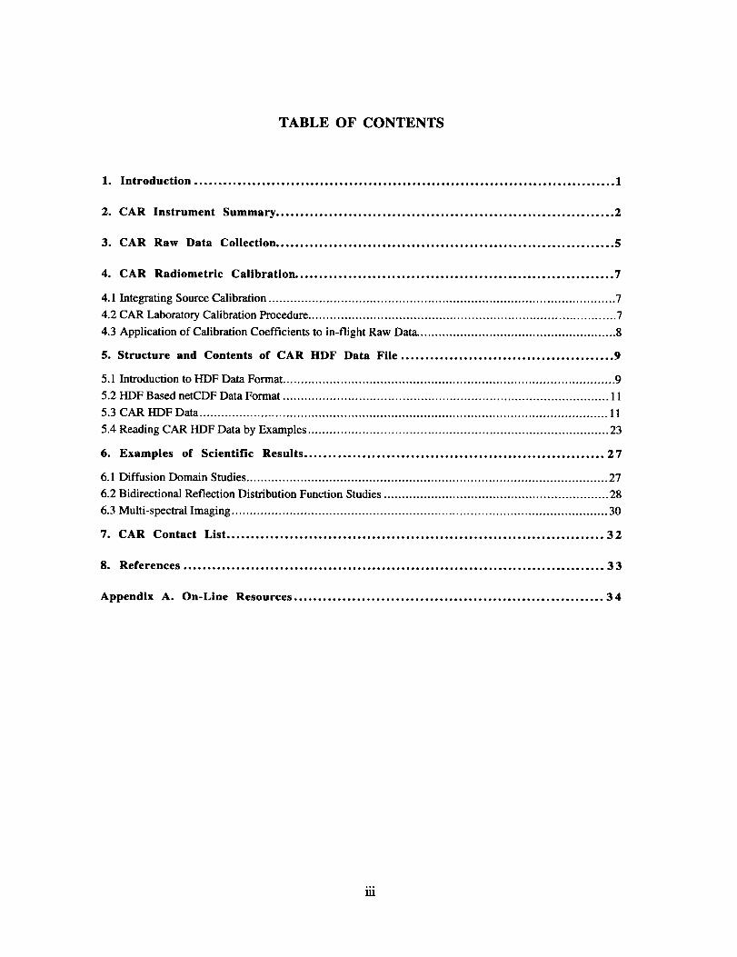
TABLE OF CONTENTS

1. Introduction ....................................................................................... 1

2. CAR Instrument Summary ...................................................................... 2

3. CAR Raw Data Collection ...................................................................... 5

4. CAR Radiometric Calibration .................................................................. 7

4.1 Integrating Source Calibration ................................................................................................ 7

4.2 CAR Laboratory Calibration Procedure ..................................................................................... 7

4.3 Application of Calibration Coefficients to in-flight Raw Data. ...................................................... 8

5. Structure and Contents of CAR HDF Data File ............................................ 9

5.1 Introduction to HDF Data Format ............................................................................................ 9

5.2 HDF Based netCDF Data Format .......................................................................................... 11

5.3 CAR HDF Data ................................................................................................................. 11

5.4 Reading CAR HDF Data by Examples ................................................................................... 23

6. Examples of Scientific Results .............................................................. 27

6.1 Diffusion Domain Studies .................................................................................................... 27

6.2 Bidirectional Reflection Distribution Function Studies .............................................................. 28

6.3 Multi-spectral Imaging ........................................................................................................ 30

7. CAR Contact List .............................................................................. 32

8. References ....................................................................................... 3 3

Appendix A. On-Line Resources ................................................................ 34

°°°

m

LIST OF FIGURES

Figure 1. Cutaway drawing of CAR ............................................................................................. 2

Figure 2. CAR instrument is housed in the nose cone of the C-131A aircraft ........................................ 4

Figure 3. An example of digital output of one CAR channel ............................................................. 5

Figure 4. CAR relative intensity as a function of scan angles in the diffusion domain (10 July 1987) ..... 27

Figure 5. To acquire BRDF data, the C-131A flies in a closed circular flight pattern ............................ 28

Figure 6. Measurements of the BRDF at 0.87 Ixm over cerrado surface (August 18, 1995) ..................... 29

Figure 7. Measurements of the BRDF at 0.87 ktm over a uniform smoke layer (September 6, 1995) ....... 29

Figure 8. Same as in Figure 7 except presented as a 3D surface plot .................................................. 30

Figure 9. CAR 0.86 _tm Eearth view image, flight 1698, September 4, 1995, SCAR-B experiment ...... 31

LIST OF TABLES

Table 1. Spectral Characteristics of CAR Channels .......................................................................... 3

Table 2. Instrumental Specifications of CAR .................................................................................. 4

Table 3. Matching CAR Data Channels With Spectral Channels ....................................................... 6

Table 4. Supported Platforms for HDF Version 4.0 ....................................................................... 10

Table 5. Cloud Absorption Radiometer Data (in alphabetical order) ................................................... 12

Table 6. Navigational and Cloud Microphysics Data (in alphabetical order) ......................................... 13

iv

1. Introduction

The Cloud Absorption Radiometer (CAR) is a multiwavelength scanning radiometer that

measures the angular distribution of scattered radiation. It was developed at NASA

Goddard Space Flight Center by Dr. Michael D. King. Originally designed to determine the

single scattering albedo of clouds at selected wavelengths in the visible and near-infrared,

the CAR has been applied to scientific problems that have evolved dramatically over the

years. Nowadays the CAR can also be used to measure bi-directional reflectance for

various surface types or simply as an imaging system. Since 1987, it has flown in the nose

cone of the Convair C-131A aircraft operated by the University of Washington, Department

of Atmospheric Sciences, in concert with an array of cloud microphysics, aerosol,

atmospheric chemistry and general meteorological instruments. CAR has been deployed on

a regular basis on experiment campaigns around the world. These have included deploy-ments to the Azores, Brazil, Kuwait, continental U.S. and Alaska.

In support of CAR related research, a CAR data processing system was designed and

implemented by the Cloud Retrieval Group at NASA Goddard Space Flight Center in early

1995. The purpose of the processing system is to ingest CAR raw data and engineering and

navigation data, and to produce calibrated radiances in a portable Hierarchical Data Format

(HDF). To complement CAR radiometric data, a set of carefully selected in situ cloud

microphysics measurements is included in the CAR HDF data set, the end product being aserf-contained and information-rich scientific data set.

The purpose of this document is to describe the CAR instrument, the methods used in the

CAR HDF data processing, the structure and format of the CAR HDF data files, and the

methods for accessing the data. Examples of CAR applications and their results are also

presented. Consult the CAR webp age at: http://climate.gsfc.nasa.gov/~jyli/CAR.html for the

most up-to-date information.

Questions about CAR HDF data should be directed to:

Jason Y. Li, CAR HDF Data ProcessingCode 913

NASA Goddard Space Flight Center

Greenbelt, MD 20771

Tel : (301) 286-1029

Fax: (301) 286-1759

Email: jyli@climate.gsfc.nasa.gov

Questions related to the Cloud Microphysics data should be addressed to:

Professor Peter V. Hobbs

Department of Atmospheric Sciences, Box 351640

University of Washington

Seattle, WA 98195-1640

Phone: (206) 543-6027; Email: phobbs@atmos.washington.edu

2. CAR Instrument Summary

The Cloud Absorption Radiometer is capable of measuring the angular distribution of

scattered radiation in thirteen spectral bands. Figure 1 shows the overall design of the

instrument with many of the mechanical, optical, and electronic components identified. The

scan minor, rotating at 100 rpm, directs the light into a Dall-Kirkham telescope, where the

beam is split into eight paths. Seven light beams pass through beam splitters, dichroics,

and lenses to individual detectors (0.30 _tm - 1.27 Ixm), and finally get registered by seven

data channels. They are sampled simultaneously and continuously. The eighth beam, on

the other hand, passes through a spinning falter wheel to a Stirling cycle cooler. Signals

registered by the eighth data channel are selected from among six spectral channels (1.55

laxn - 2.30 _rn) on the filter wheel. The filter wheel can either cycle through all six spectral

bands at a prescribed interval (usually changing filter every fourth scan line), or lock onto

any one of the six spectral bands and sample it continuously.

Electronics Cryostat

Compartment

Scan Mirrorup

Forward

//

Filter Wheel

Housing

Figure 1. Cutaway drawing of39 cm.

Telescope

SecondaryTelescope Mirror

Primary

Mirror

CAR. The dimension of the instrument housing is 72 cm x 41 cm x

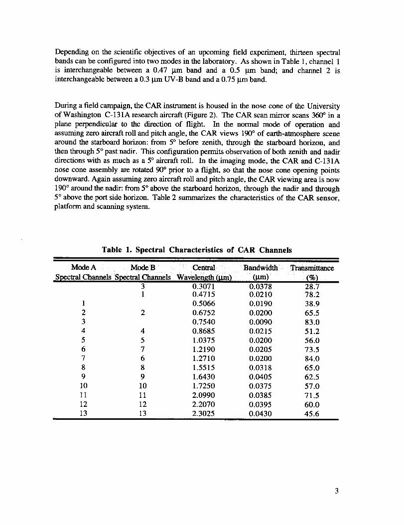
Dependingon thescientificobjectivesof an upcomingfield experiment,thirteenspectralbandscanbeconfiguredinto two modesin thelaboratory.As shownin Table1,channel1is interchangeablebetweena 0.47 Jam band and a 0.5 pan band; and channel 2 is

interchangeable between a 0.3 lxm UV-B band and a 0.75 I.tm band.

During a field campaign, the CAR instrument is housed in the nose cone of the University

of Washington C-131A research aircraft (Figure 2). The CAR scan mirror scans 360 ° in a

plane perpendicular to the direction of flight. In the normal mode of operation and

assuming zero aircraft roll and pitch angle, the CAR views 190 ° of earth-atmosphere scene

around the starboard horizon: from 5° before zenith, through the starboard horizon, and

then through 5 ° past nadir. This configuration permits observation of both zenith and nadir

directions with as much as a 5° aircraft roll. In the imaging mode, the CAR and C-131A

nose cone assembly are rotated 90 ° prior to a flight, so that the nose cone opening points

downward. Again assuming zero aircraft roll and pitch angle, the CAR viewing area is now

190 ° around the nadir: from 5 ° above the starboard horizon, through the nadir and through

5 ° above the port side horizon. Table 2 summarizes the characteristics of the CAR sensor,

platform and scanning system.

Table 1. Spectral Characteristics of CAR Channels

I I I I I

Mode A Mode B Central Bandwidth Transmittance

Spectral Channels Spectral Channels Wavelength (_) (I.tm) _%)3 0.3071 0.0378 28.71 0.4715 0.0210 78.2

1 0.5066 0.0190 38.9

2 2 0.6752 0.0200 65.5

3 0.7540 0.0090 83.0

4 4 0.8685 0.0215 51.2

5 5 1.0375 0.0200 56.0

6 7 1.2190 0.0205 73.5

7 6 1.2710 0.0200 84.0

8 8 1.5515 0.0318 65.0

9 9 1.6430 0.0405 62.5

10 10 1.7250 0.0375 57.0

11 11 2.0990 0.0385 71.5

12 12 2.2070 0.0395 60.0

13 13 2.3025 0.0430 45.6

3

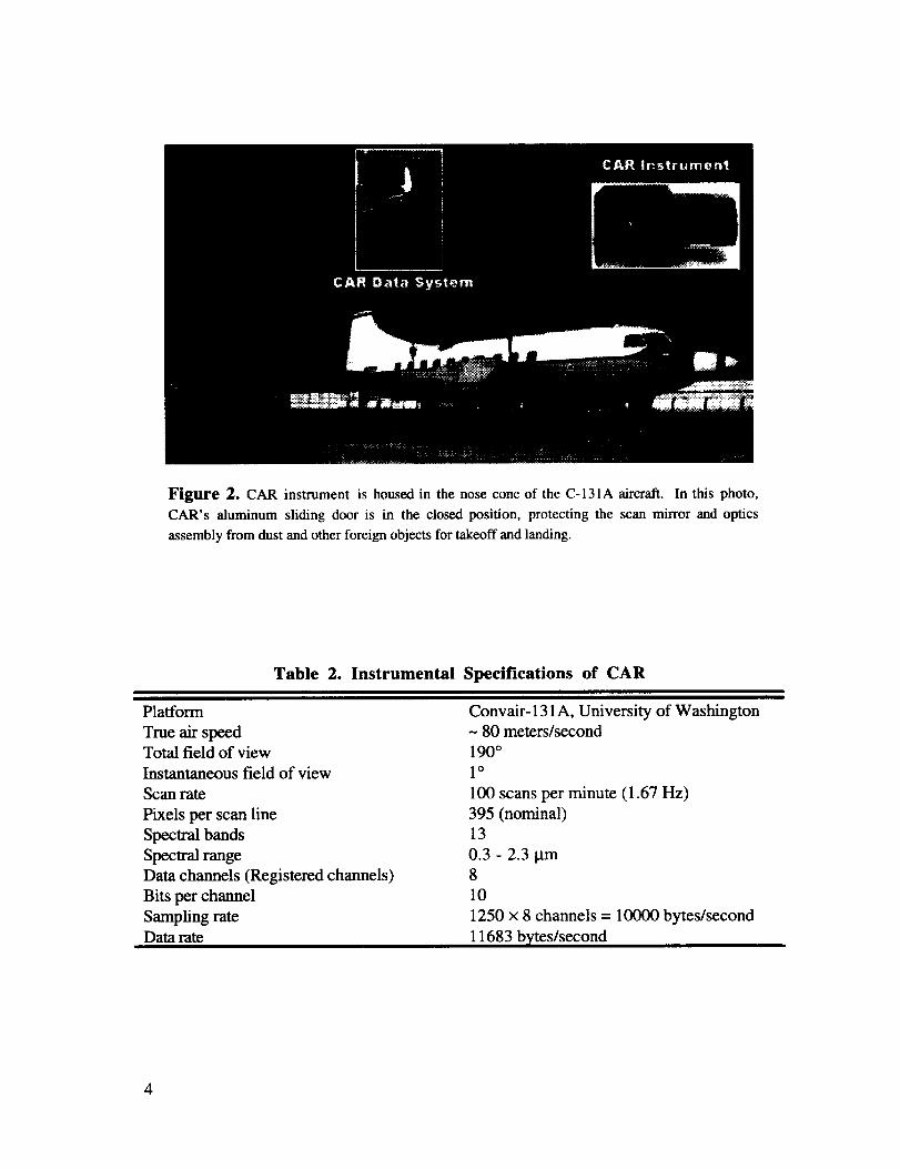
Figure 2. CAR instrument is housed in the nose cone of the C-131A aircraft. In this photo,

CAR's aluminum sliding door is in the closed position, protecting the scan mirror and optics

assembly from dust and other foreign objects for takeoff and landing.

Table 2. Instrumental Specifications of CAR

Platform

True air speedTotal field of view

Instantaneous field of view

Scan rate

Pixels per scan line

Spectral bands

Spectral range

Data channels (Registered channels)

Bits per channel

Sampling rateData rate

Convair- 131 A, University of Washington- 80 meters/second

190 °

1°

100 scans per minute (1.67 Hz)

395 (nominal)

13

0.3 - 2.3 ktm8

10

1250 x 8 channels = 10000 bytes/second

11683 bytes/second

4

3. CAR Raw Data Collection

At the beginning of each mirror scan cycle, the CAR data acquisition system first records a

ten-byte-long header. It contains information such as flight number, current time, roll

angle, scan line counter, etc. Following the header is the data stream from eight data

channels. Figure 3 shows a sample digital output of one complete scan cycle from one of

the CAR channels. Two sync pulses denote the start and end of an active scan segment.

These pulses are distinguished by their differing time durations. Assuming zero aircraft

roll and pitch angle, the CAR scan mirror should be looking at 5 ° before zenith direction at

the first pulse and 5 ° past nadir at the second pulse. Also multiplexed into each channel on

each scan cycle are the set of reference voltage, as well as the measurements from the four

thermistors. The reference voltages range from 0.00 to 8.00 V in steps of 1.00 V and give

the appearance of a staircase. This voltage staircase permits the conversion of digital

counts to voltage, while the conversion from voltage to radiances is accomplished through

the calibration procedure.

1O0

200

300

400

500

600

700

ky/Cloud

rth

5 ms active scan start

190 degree earth-atmosphere scene

10 ms active scan finish sync pulse

Eigl_t calibration stair steps"L__.

"IL_._1.-__.

¢.-.._"L-..--

'T_jIB

Four internal thermistor readings

Backside view

200 400 600 800 1000 1200

Raw Digital Counts

Figure 3. An example of digital output of one CAR channel. The limb

brightening phenomenon is a prominent feature in the CAR active scan data,

corresponding to the peak as you are seeing here.

Even though there are thirteen spectral channels available, the CAR instrument can only

output eight spectral channels of information at one time. The f'irst seven spectral channels

feed the data stream continuously. Data channel 8 collects data from one of the filter wheel

channels(spectralchannelnumber8 - 13) that is being locked on by the filter wheel at the

time. Table 3 explains how this works. Let's select arbitrarily eight consecutive scan lines

and rotate the f'flter wheel at every other scan line. The channel numbers shown in Table 3

are data channel numbers. The relationship between the first seven spectral channels and

the data channels is obvious. The matching of filter wheel and data channel 8 is entirely

dependent on the position of the filter wheel. The filter wheel can cycle through all six

spectral channels at a prescribed rate. In Table 3, only four complete cycles are shown.

When changing the filter wheel, there is no useful data to be collected by data channel 8,

which is filled with missing values. The filter wheel can be locked, that is the prescribed

filter wheel rotation rate is zero, then like the other seven data channels, the data channel 8

collects data continuously at a given near-infrared wavelength. The dwell time in the filter

wheel can be adjusted from 1 - 10 scans per filter wheel channel (automatic mode) or can

be locked into a fLxed channel position (manual mode).

Table 3. Matching CAR Data Channels With Spectral Channels

CAR

speeWalchannel

1

2

3

4

5

6

7

8

9

10

11

12

13

I

Scan Scan Scan Scan Scan Scan Scan Scan

Line Line Line Line Line Line Line Line

1 2 3 4 5 6 7 8

1 1 1 1 1 1 1 1

2 2 2 2 2 2 2 2

3 3 3 3 3 3 3 3

4 4 4 4 4 4 4 4

5 5 5 5 5 5 5 5

6 6 6 6 6 6 6 6

7 7 7 7 7 7 7 7

8 x ......

- - 8 x ....

.... 8 x - -

...... 8 x

• x changing filter* - no data

6

4. CAR Radiometric Calibration

Radiometric calibration of the CAR is conducted in the laboratory at Goddard Space Flight

Center (GSFC) both before and after use of the CAR in a field deployment. This chapter

describes how the calibration is determined and how it is applied to the raw data to convert

the raw data values to radiance. The chapter is divided into three sections. The first section

discusses the calibration of the standard integrating sources viewed by the CAR during

calibration, the second section describes the laboratory procedure used to view the

integrating sources and derive the cahbrafion coefficients to convert the CAR output signal

to radiance, and, the third section describes how to apply the calibration coefficients to in-

flight raw CAR data.

4.1 Integrating Source Calibration

Two integrating sources typically have been used for CAR calibrations: the GSFC six-foot

(183 cm) integrating sphere and the four-foot integrating hemisphere. Both sources are

internally coated with BaSO4 paint and internally illuminated by 12 quartz-halogen lamps.

Each source is calibrated by Goddard personnel, using a monochromator and reference

lamp. The monochromator consists of silicon, germanium, and lead sulfide detectors, each

of which detects narrow band radiation dispersed from their individual gratings. The

monochromator makes a relative measurement of input radiance (every 10 nm) with respect

to a reference lamp in the wavelength range from 0.4 to 2.5 btrn. The monochromator

reference lamp is traceable to a standard lamp approved by the National Institute of

Standards and Technology (NIST) and is periodically checked against other instruments

during round robin intercomparisons.

The integrating source calibration by the method just described is conducted with the

sources at maximum intensity (12 lamps on). Tests, however, also are conducted to

determine source radiance at fewer than 12 lamps. Lamps are turned off, one at a time, and

source radiance data in the wavelength range from 0.4 to 0.95 btrn is recorded. These

radiance values for each lamp level are then divided by the radiance at 12 lamps to give the

relative intensity for each lamp level. Since the relative intensity values vary less than one

percent over the wavelength range, relative intensity is considered independent of

wavelength. Thus, for each lamp level, the same relative radiance is applied regardless, of

wavelength.

4.2 CAR Laboratory Calibration Procedure

The CAR is calibrated in the laboratory at GSFC both before and after its participation in a

field experiment. The CAR is set up to view the radiometric source through an opening in

the side of the source (a 10-inch-diameter opening for the hemisphere and a 12-inch

opening for the sphere). Beginning with all 12 source lamps on, the output voltage level

7

for each of the seven gain settings for each of the 13 CAR channels is sampled in sequence

(controlled by a custom-designed "auto-calibrator" box). The sampling consists of

averaging a selected portion of the output voltage level of each scan (when viewing the

source) for about 30 scans. Each sample is digitized and written to a computer disk file.

This procedure is repeated for each lamp level. Thus, for each gain setting of each CAR

channel, calibration coefficients (slope and intercept) are computed from linear regression

of the CAR-measured voltage at each lamp level, and the corresponding radiance values

(source radiance at the central wavelength of each channel). Analysis of the calibration

coefficients shows that the slope values for each channel are independent of gain setting

(though the offset usually varies slightly with gain setting).

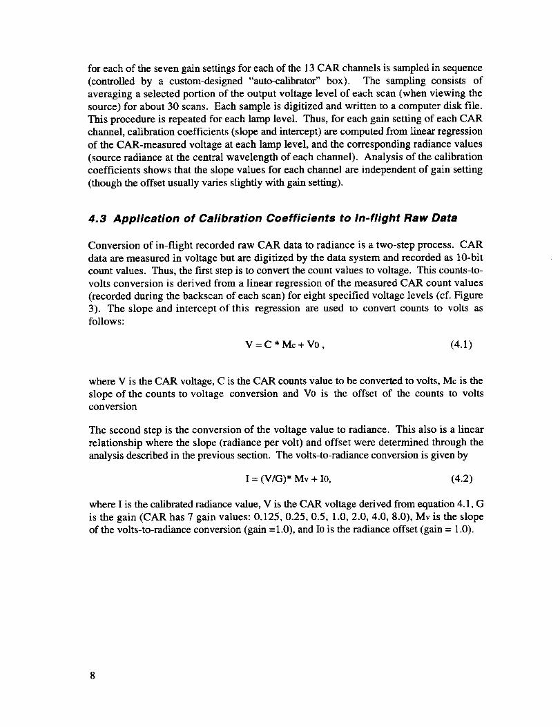
4.3 Application of Calibration Coefficients to In-flight Raw Data

Conversion of in-flight recorded raw CAR data to radiance is a two-step process. CAR

data are measured in voltage but are digitized by the data system and recorded as 10-bit

count values. Thus, the In'st step is to convert the count values to voltage. This counts-to-

volts conversion is derived from a linear regression of the measured CAR count values

(recorded during the backscan of each scan) for eight specified voltage levels (cf. Figure

3). The slope and intercept of this regression are used to convert counts to volts as

follows:

V = C * Mc + V0, (4.1)

where V is the CAR voltage, C is the CAR counts value to be converted to volts, Mc is the

slope of the counts to voltage conversion and V0 is the offset of the counts to voltsconversion

The second step is the conversion of the voltage value to radiance. This also is a linear

relationship where the slope (radiance per volt) and offset were determined through the

analysis described in the previous section. The volts-to-radiance conversion is given by

I = (V/G)* Mv + I0, (4.2)

where I is the calibrated radiance value, V is the CAR voltage derived from equation 4.1, G

is the gain (CAR has 7 gain values: 0.125, 0.25, 0.5, 1.0, 2.0, 4.0, 8.0), Mv is the slope

of the volts-to-radiance conversion (gain =1.0), and I0 is the radiance offset (gain = 1.0).

5. Structure and Contents of CAR HDF Data File

5.1 Introduction to HDF Data Format

HDF stands for Hierarchical Data Format and was created at the National Center for Super-

computing Applications (NCSA). HDF is a multiobject file format for the transfer of

graphical and numerical data between machines. It supports six different data models:

• 8-bit raster images

• 24-bit raster images

• color palettes• text annotation

• binary table (Vdata model)

• scientific data sets model (SDS model)

Each data model defines a specific type of data and provides a convenient interface for

reading, writing, and organizing a unique set of data elements. In a sense, the word HDF

carries dual meanings: it is an interface to a library of data access programs that store andretrieve HDF file format data.

I data sets are stored as HDF SDS-based _I InetCDF data ob'ectsIIIIIIII II III II II I IIIII I III II IIIII II I I I II IIIII II II I III I I III I I I

There are numerous advantages of storing data in general purpose HDF format over any

"purpose specific" format. Just name a few:

• HDF is a self-describing format, allowing an application to interpret the contents of a

file without any outside information. From a programmer's point of view, parameters

in an HDF file are retrieved by their names, not by their physical locations in the file.

Unlike working with purpose specific data formats, you do not need to know the

structural details of an HDF file. In addition to meaningful parameter names, the self-

describing capability is further enhanced by adding the parameter attributes or name

tags, such as parameter physical units, scale factors and missing values.

HDF is a portable file format, sometimes described as a network transparent file

format. Usually different computer architectures have different ways of representing

integers and floating-point numbers. In order to read a binary file on a different

computer platform, for example, you need to resolve issues like byte ordering and the

position of the most and least significant bytes. With HDF, these things are all taken

care of by the HDF library. HDF files can be shared across platforms. An HDF file

created on one computer, say a Cray supercomputer, can be read on another system,

say an IBM PC, without modification. HDF library does all the hard work for you

9

behindthe scene.A full list of HDF (version4.0 release2) supportedplatformsarepresentedin Table4.

HDF is available in thepublic domainandis fully supportedby NCSA. You canobtain anHDF softwarepackage,a usermanual,anda referencemanualby anony-mousftp on Internet at ftp.ncsa.uiuc.edu (141. 142.21.14) . There is also a

galaxy of information on the NCSA's HDF Information Server (world wide web site)

at http : //hdf. ncsa. uiuc. edu/. To join in the discussions of various common data

file formats, Usernet newsgroup sci. data. formats may be a good place to visit.

And of course you can send any comments or suggestions to HDF user support by E-

mailathdfhelp@ncsa, uiuc. edu.

Table 4. Supported Platforms for HDF Version 4.0

PlafforwJOperating System

II

Basic HDF Library HDFbaetCDF Library

libdf, a libmfhdf, a

Sun4/SunOS 4.1.3

Sun4/Solaris 2.4 - 2.5

SGI-Indy/IRIX5.3

SGI/IRIX6. l_n32bit

SGI/IRIX6. l_64bit

HP9000/HPUX9.03

Cray Y-MP/UNICOS 803.2

Cray C90/UNICOS 803.2

Thinking Machine CM5IBM RS6000/AIX v4.1

IBM SP2

DEC Alpha/Digital Unix v3.2

DEC Alpha/Open VMS AXP v6.2

Fjujitsu UXP/UXPMIBM PC/Solarisx86

IBM PC/Linux vl.2.4

IBM PC/Linux elf 1.2.13

IBM PC/FreeBSD 2.0

Windows NT/95

PowerPC/Mac OS 7.5

VAX/VMS

Yes Yes

Yes Yes

Yes Yes

Yes Yes

Yes Yes

Yes Yes

Yes Yes

Yes Yes

Yes Yes

Yes Yes

Yes Yes

Yes Yes

Yes Yes

Yes Yes

Yes Yes

Yes Yes

Yes Yes

Yes Yes

Yes Yes

Yes Yes

No No

10

5.2 HDF-Based netCDF Data Format

Like HDF, netCDF (network Common Data Form) is another very popular interface to a

library of data access programs that store and retrieve data. The netCDF file format is also

self-describing and network-transparent. It was developed by the Unidata Program Center,

University Corporation for Atmospheric Research (UCAR) in Boulder, Colorado. The

original intent was to provide U.S. universities a common data access method for the

various Unidata applications. While HDF has six sets of interfaces supporting six data

models, netCDF, on the other hand, has only one set of interface for supporting one data

model. The counterpart of netCDF in HDF is the multifile Scientific Data Sets (SDS).

Then what is the HDF-based netCDF data format? As alluded to in the preceding section,

CAR data are stored as HDF SDS-based or encoded netCDF objects. To understand the

connection between HDF SDS and netCDF objects, we have to look back to the history of

their developments. HDF and netCDF were created independently by two research

organizations. Despite their similarities, in the early days the HDF SDS interface could not

read a netCDF object or vice versa. However, this predicament has changed recently,

thanks to the cooperative spirit between the HDF development group at NCSA and the

netCDF group at UCAR. From HDF version 3.3, HDF SDS interface supports complete

netCDF interface as defined by Unidata netCDF Release 2.3.2, and the netCDF data format

is interchangeable with the HDF SDS data model in so far as it is possible to use the

netCDF calling interface to place an SDS into an HDF file. Nowadays, using either

interface (HDF SDS or netCDF), you are able to read HDF SDS based netCDF files (such

as our Cloud Absorption Radiometer HDF files), pre-HDF 3.3 HDF files and XDR °-

based netCDF files. The HDF/netCDF library provided by NCSA identifies what type of

file is being accessed and handles it appropriately. It is completely transparent to the

programmers. In section 5.4, we will show you how to retrieve HDF SDS-based netCDF

objects using either interfaces in FORTRAN, C, or IDL programming languages.

If you choose the netCDF interface to read HDF-based netCDF files, the netCDF User's

Guide is indispensable. A postscript version of the user's guide can be obtained by anony-

mous ftp at _:tp.unidata.ucar. edu. It is also available on the Internet as an HTML

document athttp ://unidata. ucar. edu/packages/netcdf /index. html.

5.3 CAR HDF Data

The contents of a CAR HDF data set are primarily made up of three components: calibrated

CAR radiance data, aircraft navigational data, and a suite of CAR research relevant to cloud

microphysics data. The latter two data sets are maintained and distributed by the Cloud and

"XDR stands for eXternal Data Representation. XDR, developed by Sun Microsystems Inc, is a non-

proprietary standard for describing and encoding data. It supports encoding arbitrary C data structures into

machine-independent sequences of bits. The encoding used for floating-pint numbers is the IEEE standard

for normalized floating-pint numbers.

11

Aerosol Research Group, University of Washington. Data dimensions, physical units, and

missing values of every variable in the CAR HDF data set are listed in Table 5 and 6.

Table 5. Cloud Absorption Radiometer Data (in alphabetical order)

.... ..................... .mrsCAR Parameters _on Value

AmplifierGain time

BasePlateTemperature time Celsius

BeforeNadirlndex time

CalibratedData (410, 8, time) watts/m2/steradiard_ma

Calibrafionlntercept 13 watts/m2/steradian/lan

CalibrationSlope 13 watts/m2/steradian/lam/volt

CarRoll time degree

CenteralWavelength 13 lam

Coordinated Universal Time time HHMMSS

CountsVoltagelntercept time volts

CountsVoltageSlope time Volts/count

DoorOpenStatus time

FilterWheelChannel time

FilterWheelPosition time

LongwaveDataGood time

ManualGainControl time

NumberOfScanPixels 410

Optics 1Temperature time Celsius

Optics2Temperature time Celsius

PastZenith/ndex time

PrirnaryMirrorTemperature time Celsius

ScanAnglel time degree

ScanLineCounter time

ScanMirrorCondensationFlag time

SolarAzimuthAngle time degree

SolarSpectrallrradiance 13 watts/meter2/micron

SolarZenithAn_le time de_;_ee

-32768

-32768

-32768

-99999.0

-99999.0

12

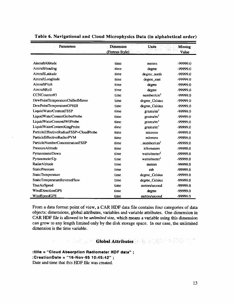
Table 6. Navigational and Cloud Microphysics Data (in alphabetical order)

Parameters Dimension

........ ........ Value

AircraflAltitude

AircraftHeading

AircraftLatitude

AircraRLongitude

AircraftPitch

AircraftRoll

CCNCounter#3

DewPointTemperatureChiUedMirror

DewPointTemperatureOPHIR

LiquidWaterContentFS SP

LiquidWaterContentGerberProbe

LiquidWaterC ontentlWOProbe

LiquidWaterContentKingProbe

PanicleEffectiveRadiusFSSP+CloudProbe

ParticleEffectiveRadiusPVM

ParticleNumberConcentrationFSSP

PressureAltitude

PyranometerDown

PyranometerUp

RadarAltitude

StaticPressure

StaticTemperature

StaticTemperatureReverseFlow

TmeAirSpeed

WindDirectionGPS

WindSpeedGPS

time meters -99999.0

time degree -99999.0

time degree_north -99999.0

time degree_east -99999.0

time degree -99999.0

time degree -99999.0

time number/cm 3 -99999.0

time degreeCelsius -99999.0

time degree_Celsius -99999.0

time grams/m 3 -99999.0

time grams/m 3 -99999.0

time grams/m 3 -99999.0

time grams/m 3 -99999.0

time microns -99999.0

time microns -99999.0

time . number/cm a -99999.0

time kilometers -99999.0

time watts/meter: -99999.0

time watts/meter _ -99999.0

time meters -99999.0

time mb -99999.0

time degree_Celsius -99999.0

time degree_Celsius -99999.0

time meters/second -99999.0

time degree -99999.0

time meters/second -99999.0

From a data format point of view, a CAR HDF data file contains four categories of data

objects: dimensions, global attributes, variables and variable attributes. One dimension in

CAR HDF file is allowed to be unlimited size, which means a variable using this dimension

can grow to any length limited only by the disk storage space. In our case, the unlimiteddimension is the time variable.

:title = "Cloud Absorption Radiometer HDF data" ;

:CreationOate = "16-Nov-95 10:45:42" ;

Date and time that this HDF f'de was created.

13

:CreatedBy = "Jason Li (jyli@climate.gsfc.nasa.gov)" ;Person who created this CAR HDF file.

:SoftwareVersion = "Version 3.2" ;

HDF data processing software version number.

:Credits = "J. Y. Li, H. G. Meyer, G. T. Arnold, S. C. Tsay and M. D. King";

:ExperimentName = "SCAR-B 1995" ;Name of CAR mission.

:FlightDate = " 4 Sep 1995";

Beginning date of CAR flight.

:CarViewingMode = "Downward" ;

Specify how the CAR is being mounted in the nose cone of the host aircraft. The normal

viewing mode is to scan around the starboard horizon.

:CarOperatorComment = "CAR used as an imager; On transit from Cuiaba to

Vilhena, coordinated flight with ER-2 NW of Cuiaba; Fairly uniform aerosol onclimbout; Clouds dissipated W/NW of Cuiaba. Also see SCAR-B CAR Flight

Log by Jason Li, NASA Goddard Space Flight Center." ;

Character string records CAR operator's flight summary.

:LocalTimeOffset = -4s ;

Difference between local time and UTC, expressed in hours. Postive is for the regions east

of Greenwich meridian and negative for the west. Add LocalTimeOffset to the UTC time,

you get the local time.

:JulianDay = 247s ;

Number of days since the first day of the year, not the Julian date concept defined by

Astronomical community.

:FlightNumber = 1698s ;

C 131A flight number assigned by University of Washington.

:data_set = "Cloud Absorption Radiometer HDF Data" ;

:data_product = "Flight Track" ;

:sensor = "Cloud Absorption Radiometer" ;

:platform = "Convair C-131A" ;Host aircraft name.

14

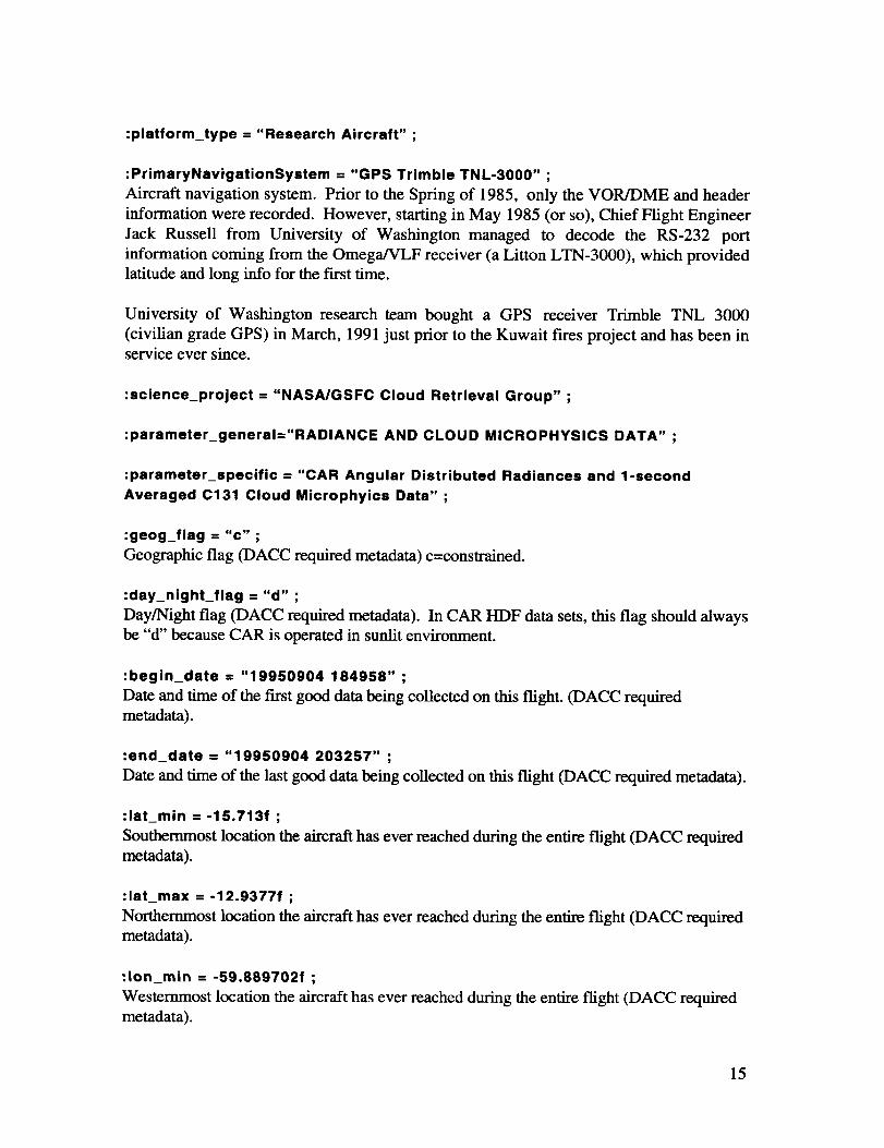
:platform_type = "Research Aircraft" ;

:PrimaryNavigationSystem = "GPS Trimble TNL-3000" ;

Aircraft navigation system. Prior to the Spring of 1985, only the VOR/DME and header

information were recorded. However, starting in May 1985 (or so), Chief Flight Engineer

Jack Russell from University of Washington managed to decode the RS-232 port

information coming from the Omega/VLF receiver (a Litton LTN-3000), which provided

latitude and long info for the first time.

University of Washington research team bought a GPS receiver Trimble TNL 3000

(civilian grade GPS) in March, 1991 just prior to the Kuwait fires project and has been inservice ever since.

:science_project = "NASA/GSFC Cloud Retrieval Group" ;

:parameter_general="RADIANCE AND CLOUD MICROPHYSICS DATA" ;

:parameter_specific = "CAR Angular Distributed Radiances and 1-second

Averaged C131 Cloud Microphyics Data" ;

:geog_flag = "c" ;

Geographic flag (DACC required metadata) c=constrained.

:day_night_flag = "d" ;

Day/Night flag (DACC required metadata). In CAR HDF data sets, this flag should always

be "d" because CAR is operated in sunlit environment.

:begin_date = "19950904 184958" ;

Date and time of the first good data being collected on this flight. (DACC required

metadata).

:end_date = "19950904 203257" ;

Date and time of the last good data being collected on this flight (DACC required metadata).

:lat_min = -15.713f ;

Southernmost location the aircraft has ever reached during the entire flight (DACC required

metadata).

:lat_max = -12.9377f ;

Northernmost location the aircraft has ever reached during the entire flight (DACC requiredmetadata).

:Ion_rain = -59.889702f ;

Westernmost location the aircraft has ever reached during the entire flight (DACC required

metadata).

15

:Ion_max = -56.1628f ;

Easternmost location the aircraft has ever reached during the entire flight (DACC required

metadata).

Dimensions

time = UNLIMITED ; H (10335 currently)The unlimited dimension in the CAR HDF data set is the time dimension. It can also be

understood as number of scan lines in the CAR HDF data file.

NumberOfPixels = 410 ;

Maximum number of scan pixels per scan line.

NumberOfChannels = 13 ;

Number of CAR spectral channels.

NumberOfDataChannels = 8 ;

Number of CAR data channels. Seven of them are sampled simultaneously and

continuously, and the remaining data channel is fed from one of the six spectral channels

on the CAR filter wheel channel.

Variables and Their Attributes

long CoordinatedUniversalTime(time) ;CAR time code in UTC (HHMMSS format). CAR instrument does not have its own time

code generator. The C 131 master clock feeds time information to CAR data stream on a 1-second carrier wave. Therefore the CAR time code resolution is truncated to a second.

Recall the CAR sampling rate is 1.67 Hz, the scan mirror may have completed two scans,

while the clock reading remains unchanged.

long ScanLineCounter(time) ;Number of scan mirror revolutions. The ScanLineCounter starts at 1 when the CAR

instrument is powered on. However, a CAR operator often does not activate the data

recording system until the CAR filterwheel channels are cooled sufficiently for better

signal-to-noise ratio. The initial value of ScanLineCounter in an HDF file is usually on theorder of hundreds.

float CentralWavelength(NumberOfChannels) ; CentralWavelength:units ="microns" ;

CAR channel central wavelength in microns.

16

float SolarSpectrallrradiance(NumberOfChannels) ;

SolarSpectrallrradiance:units = "watts/meter2/micron" ;

Solar spectral irradiance at top of the atmosphere for each CAR channel.

computed using LOWTRAN code.

They are

short FilterWheelPosition(time) ;

FilterWheelPosition:missing_value = -32768s ;

It can take an integer value between 1 and 6, corresponding to 6 filters on the fdterwheel.

A missing value of -32768 indicates the filterwheel is in the middle of changing filter.

short LongwaveDataGoodFlag(time) ;Engineering data; 0 for good, otherwise 1.

short ScanMirrorCondensationFlag(time) ;

Scan mirror condensation indicator; 0 for no condensation, otherwise 1.

short ManualGsinControl(time) ;

Manual gain control setting. Presently, there are 7 different gain settings (from 0 to 6)

available, corresponding to amplification gain range from one-eighth to eight times.

short DoorOpenStatus(time) ;

Engineering data; 0 for door close and 1 for door open status. In CAR HDF data sets,

CAR door should always be open.

short FilterWheelChannel(time) ;

FilterWheelChannel:missing_value = -32768s ;

It indicates which filterwheel channel is being used at the moment. Filterwheel channelnumber is between 8 and 13.

float AircraftLatitude(time) ;

AircraftLatitude:units = "degree_north" ;

AircraftLatitude:missing_value = -99999.f ;

Aircraft subpoint latitude. Positive values are for locations in the northern hemisphere;

negative values, for locations in the southern hemisphere. They are derived from whichever

primary navigational system is being used at the time of the flight, usually GPS system.

float AircraftLongitude(time) ;

AircraftLongitude:units = "degree_east" ;

AircraftLongitude:missing_value = -99999.f

Aircraft subpoint longitude. Positive values are for locations east of Greenwich meridian;

negative values for locations west of Greenwich meridian. They are derived from

whichever the primary navigational system is being used at the time of the flight, usually

GPS system.

float AircraftHeading(time) ;

AircraftHeading:units = "degree" ;

17

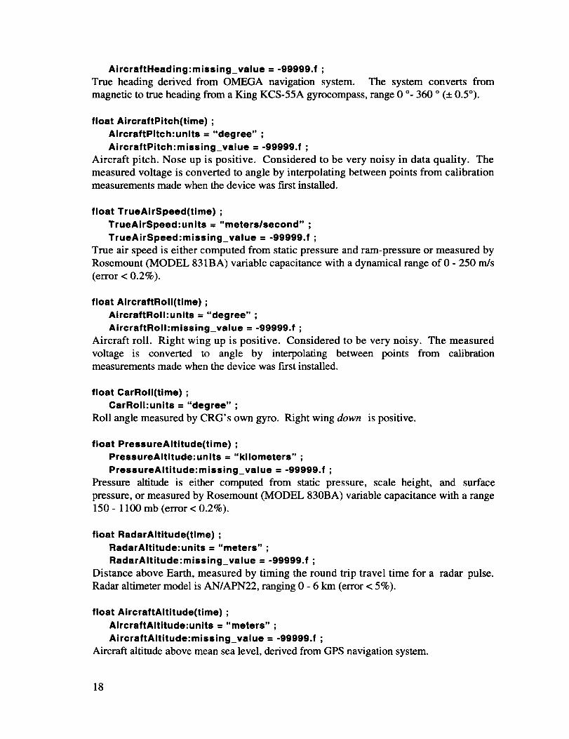
AircraftHeading:missing_value = -99999.f ;

True heading derived from OMEGA navigation system. The system converts from

magnetic to true heading from a King KCS-55A gyrocompass, range 0 °- 360 ° (± 0.5°).

float AircraftPitch(time) ;

AircrsftPitch:units = "degree" ;

AircraftPitch:missing_value = -99999.f ;

Aircraft pitch. Nose up is positive. Considered to be very noisy in data quality. The

measured voltage is converted to angle by interpolating between points from calibrationmeasurements made when the device was first installed.

float TrueAirSpeed(time) ;

TrueAirSpeed:units = "meters/second" ;

TrueAirSpeed:missing_value = -99999.f ;

True air speed is either computed from static pressure and ram-pressure or measured by

Rosemount (MODEL 831BA) variable capacitance with a dynamical range of 0 - 250 rrds

(error < 0.2%).

float AircraftRoll(time) ;

AircraftRoll:units = "degree" ;AircraftRoll:missing_value = -99999.f ;

Aircraft roll. Right wing up is positive. Considered to be very noisy. The measured

voltage is converted to angle by interpolating between points from calibrationmeasurements made when the device was first installed.

float CarRoll(time) ;

CarRoll:units = "degree" ;

Roll angle measured by CRG's own gyro. Right wing down is positive.

float PressureAItitude(time) ;PressureAItitude:units = "kilometers" ;

PreasureAItitude:missing_value = -99999.f ;

Pressure altitude is either computed from static pressure, scale height, and surface

pressure, or measured by Rosemount (MODEL 830BA) variable capacitance with a range

150 - 1100 mb (error < 0.2%).

float RadarAItitude(time) ;RadarAItitude:units = "meters" ;

RadarAItitude:missing value = -99999.f ;

Distance above Earth, measured by timing the round trip travel time for a radar pulse.

Radar altimeter model is AN/APN22, ranging 0 - 6 km (error < 5%).

float AircraftAItitude(time) ;

AircraftAItitude:units = "meters" ;

AircraftAItitude:missing_value = -99999.f ;

Aircraft altitude above mean sea level, derived from GPS navigation system.

18

float StaticPressure(time) ;

StaticPressure:units = "mb" ;

StaticPressure:missing_value = -99999.f ;

Static pressure in millibars measured by Rosemount model 830BA pressure transducer.

float StaticTemperature(time) ;

StaticTemperature:units = "degree_Celsius" ;StaticTemperature:missing_value = -99999.f ;

Static temperature is measured directly by the deiced Rosemount probe.

float StaticTemperatureReverseFIow(time) ;

StaticTemperatureReverseFIow:units = "degree_Celsius" ;

StaticTemperatureReverseFIow:missing_value = -99999.f ;

Static temperature measured by probe developed in house at University of Washington. It

uses special housing to reverse the air flow in order to reduce the dynamic heating and

evaporative cooling by cloud liquid water.

float WindSpeedGPS(time) ;

WindSpeedGPS:units = "meters/second" ;

WindSpeedGPS:missing_value = -99999,f ;

Wind speed computed from the GPS ground track, GPS ground speed, OMEGA heading,

and aircraft true air speed.

float WindDirectionGPS(time) ;

WindDirectionGPS:units = "degree" ;

WindDirectionGPS:missing_value = -99999.f ;

Wind speed computed from the GPS ground track, GPS ground speed, OMEGA heading

and aircraft true air speed. Direction is where the wind is coming from.

float CCNCounter#3(time) ;

CCNCounter#3:units = "number/cm3" ;

CCNCounter#3:missing_value = -99999.f ;Cloud condensation nuclei counter #3. General Electric TSI Model 3070, connected to TSI

Model 3040 diffusion battery. The computer counts the nuclei. Only the counts from the

zero port are returned. CNC #3 sometimes is removed for use by another instrument (the

DMPS).

float ParticleNumberConcentrationFSSP(time) ;ParticleNumberConcentrationFSSP:units = "number/cm3" ;

ParticleNumberConcentrationFSSP:missing_value = -99999.f ;

Particle number concentration based on Forward Scattering Spectrometer Probe.

float LiquidWaterContentJW0Probe(time) ;

LiquidWaterContentJW0Probe:units = "grams/meter3" ;

LiquidWaterContentJW0Probe:missing_value = -99999.f ;

Liquid water content--zero drift adjusted (Johnson-Williams).

19

float LiquidWaterContentGerberProbe(time) ;

LiquidWaterContentGerberProbe:unita = "grams/meter3" ;

LiquidWaterContentGerberProbe:missing_value = -99999.f ;

Liquid water content - measured by Gerber probe.

float LiquidWaterContentKingProbe(time) ;

LiquidWaterContentKingProbe:units = "grams/meter3" ;

LiquidWaterContentKingProbe:missing_value = -99999.f ;

Liquid water content - measured by King probe.

float LiquidWaterContentFSSP(time) ;

LiquidWaterContentFSSP:units = "grams/meter3" ;

LiquidWaterContentFSSP:missing_value = -99999.f ;

Liquid water content - measured by Forward Scatering Spectrometer Probe.

float ParticleEffectiveRadiusFSSP+CIoudProbe(time) ;

ParticleEffectiveRadlusFSSP+CIoudProbe:units = "microns" ;

ParticleEffectiveRadiusFSSP+CIoudProbe:missing_value = -99999.f ;

Particle effective radius computed from measured size spectra of FSSP and cloud probe.

float ParticleEffectiveRadiusPVM(time) ;

ParticleEffectiveRadiusPVM:units = "microns" ;

ParticleEffectiveRadiusPVM:missing_value = -99999.f ;

Particle effective radius measured by Gerber PVM probe.

float DewPointTemperatureOPHIR(time) ;

DewPointTemperatureOPHIR:units = "degree_Celsius" ;

DewPointTemperatureOPHIR:missing_value = -99999.f ;

Dew point temperature determined by Ophir Corp instrument.

float DewPointTemperatureChilledMirror(time) ;

DewPointTemperatureChilledMirror:units = "degree_Celsius" ;

DewPointTemperatureChilledMirror:missing_value = -99999.f ;

Cooled mirror dew point temperature measured by Cambridge TH73-244 instrument, with

a range of -40 ° - +40 ° (error < 1°).

float PyranometerUp(time) ;

PyranometerUp:units = "watts/meter2" ;

PyranometerUp:missing_value = -99999.f ;

Upward looking pyranometer; Epply thermopile Model PSP.

float PyranometerDown(time) ;

PyranometerDown: units = "watts/meter2" ;

PyranometerDown:missing_value = -99999.f ;

Downward looking pyranometer; Epply thermopile Model PSP.

20

float SolarZenithAngle(time) ;

SolarZenithAngle:units = "degree" ;

SolarZenithAngle:missing_value = -99999.f ;

Solar zenith angle computed based on Smithsonian Meteorological Tables.

float SolarAzimuthAngle(time) ;

SolarAzimuthAngle:units = "degree" ;

SolarAzimuthAngle:missing_value = -99999.f ;

Solar azimuth angle computed based on Smithsonian Meteorological Tables.

short Optics 1Temperatu re(time) ;OpticslTemperature:units = "degree_Celsius" ;

OpticslTemperature:scale_factor = 0.0099999998f ;

Instrument temperature of optics assembly B = Optics�Temperature * scale_factor.

short Optics2Temperature(time) ;

Optics2Temperature:units = "degree_Celsius" ;Optics2Temperature:scale_factor = 0.0099999998f ;

Instrument temperature of optics assembly C = Optics2Temperature * scale_factor.

short PrimaryMirrorTemperature(time) ;PrimaryMirrorTemperature:units = "degree_Celsius" ;

PrimaryMirrorTemperature:scale_factor = 0.0099999998f ;

Primary mirror temperature = PrimaryMirrorTemperature * scale_factor

short BasePlateTemperature(time) ;

BasePlateTemperature:units = "degree_Celsius" ;BasePlateTemperature:scale_factor = 0.0099999998f ;

Baseplate temperature = BasePlateTemperature * scale_factor

float CountsVoltageSIope(time) ;CountsVoltageSIope:units = "volts/count" ;

Raw counts-to-voltage conversion slope. It is determined for each scan line and is used in

the counts to radiance conversion process.

float CountsVoltagelntercept(time) ;CountsVoltagelntercept:units = "volts" ;

Raw counts-to-voltage conversion intercept. It is determined for each scan line and is used

in the counts to radiance conversion process.

float CalibrationSIope(NumberOfChannels) ;

CalibrationSIope:units = "watts/meter2/steradian/micron/volt" ;

Voltage-to-radiance conversion slope. It is obtained from laboratory radiometric calibration

procedure and is used in the counts-to-radiance conversion process.

21

float Calibretionlntercept(NumberOfChennels) ;

Calibrationlntercept:units = "wetts/meter2/steredian/micron" ;

Voltage to radiance conversion intercept. It is obtained from laboratory radiometric

calibration procedure and is used in the counts-to-radiance conversion process.

short AmplifierGain(time) ;

AmplifierGain:scale_factor = 0.001f ;

Amplification gain factor = AmplifierGain * Scale_factor. It is used in the counts to

radiance conversion process.

short NumberOfScanPixels(time) ;

Number of active scan pixels. It is used in determining the scan angle of each scan pixel.

short PastZenithlndex(time) ;

PaetZenithlndex:missing_vslue = -32768s ;

Pixel number for the first pixel past zenith. So the local zenith is somewhere between this

pixel and previous one.

short BeforeNadirlndex(time) ;

BeforeNadirlndex:missing_value = -32768s ;

Pixel number for the last pixel just before nadir. So the local nadir is somewhere between

this pixel and the next one.

float ScanAnglel(time) ;

ScsnAnglel :units = "degree" ;

Scan angle for the first active scan pixel. It is used in determining the scan angle for each

scan pixel. Thus the scan angle for i thpixel (0i) in an active scan can be determined by

0i = 00 + ( i - 1) * 190.0 / (N - 1), (5.1)

where:

i=1,2 ....... N

01 = ScanAnglelN = NumberOfScanPixels

short CelibratedData(time, NumberOfRegisteredChsnnels, NumberOfPixels)

CslibratedDsta:scale_factor = 0.19561617f, 0.28452677f, 0.41445029f,

0.090800203f, 0.13710038f, 0.049314979f, 0.034395352f, 0.049673285f ;CalibratedData:units = "watts/meter2/steradian/micron" ;

CalibratedData:missing_value = -32768s ;Calibrated radiance values = CalibratedData * scale_.factor

The calibrated radiance values are related to the raw digital counts by the following

relationship:

radiance = (1 / Gain) * [ Ivz_ + Svzr * (C - Ic2v) / Sczv], (5.2)

22

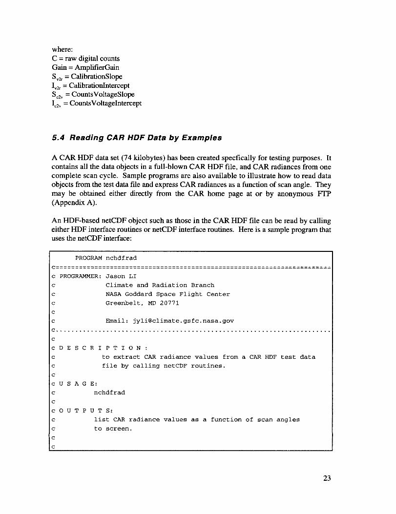
where:C = raw digital counts

Gain = AmplifierGain

Sv2_ = CalibrationSlope

Iv2_ = Calibrationlntercept

Sc2_ = CountsVoltageSlope

Ic2_ = CountsVoltagelntercept

5.4 Reading CAR HDF Data by Examples

A CAR HDF data set (74 kilobytes) has been created specfically for testing purposes. It

contains all the data objects in a full-blown CAR HDF file, and CAR radiances from one

complete scan cycle. Sample programs are also available to illustrate how to read data

objects from the test data file and express CAR radiances as a function of scan angle. They

may be obtained either directly from the CAR home page at or by anonymous PTP

(Appendix A).

An HDF-based netCDF object such as those in the CAR HDF file can be read by calling

either HDF interface routines or netCDF interface routines. Here is a sample program thatuses the netCDF interface:

PROGRAM nchdfrad

c

c

c

c

c

c

c

PROGRAMMER: Jason LI

Climate and Radiation Branch

NASA Goddard Space Flight Center

Greenbelt, MD 20771

Email: jyli@climate.gsfc.nasa.gov

C°°,.o,o..,,,,o.o,,,..oo,oo,°,o,,,o,o,,,o,oo,.ooooo°°.o°.o...o,,.,,,.,o°

C

c

c

c

c

:C

;C

D E S C R I P T I ON :

to extract CAR radiance values from a CAR HDF test data

file by calling netCDF routines.

USAGE:

nchdfrad

cOU

c

c

c

c

P U T S:

list CAR radiance values

to screen.

as a function of scan angles

23

C LANGUAGE :

c FORTRAN compiled on SGI Indigo running IRIX 6.2

c I used makefile "f77nchdfrad.mak" to compile the program.

c

cHISTORY:

c

c SLog: nchdfrad.f,v $

c Revision i.i 1997/02/07 02:39:56 jyli

c Initial revision

c

c

IMPLICIT NONE

INCLUDE '/usr/local/include/netcdf.inc'

integer

real

numberPixels, numberDataChannels

aperture

parameter (numberPixels = 410, numberDataChannels = 8)

parameter (aperture = 190.0)

character hdfFilename*12

integer recordNumber

integer

&

&

i, j, k, hdfid, varid, slcid, pixid, angid, iret

scanLineCounter

start(3), count(3)

integer*2 numberScanPixels, missing

& , calibratedData(numberPixels, numberDataChannels)

real

&

&

&

delta, scanAnglel, badData

• scanAngles(numberPixels)

, radiance(numberDataChannels)

, scalefac(numberDataChannels)

data hdfFilename /'test.hdf'/

data recordNumber/i/

data badData/-999.0/

! input HDF filename

! input record number

c set proper HDF error handling characteristics:

call ncpopt( NCVERBOS + NCFATAL )

c

c... open an existing HDF file with READONLY mode turned on:

24

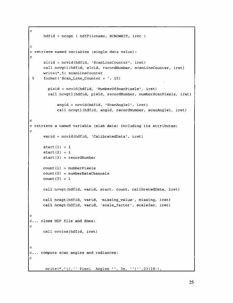
hdfid = ncopn ( hdfFilename, NCNOWRIT, iret )

c

c retrieve named variables (single data value):

c

slcid = ncvid(hdfid, 'ScanLineCounter', iret)

call ncvgtl(hdfid, slcid, recordNumber, scanLineCounter, iret)

write(*,5) scanLineCounter

5 format('Scan_Line_Counter = ', i5)

pixid = ncvid(hdfid, 'NumberOfScanPixels', iret)

call ncvgtl(hdfid, pixid, recordNumber, numberScanPixels, iret)

angid = ncvid(hdfid, 'ScanAnglel', iret)

call ncvgtl(hdfid, angid, recordNumber, scanAnglel, iret)

c

c retrieve a named variable (slab data) including its attributes:

c

varid = ncvid(hdfid, 'CalibratedData', iret)

start(l) = 1

start(2) = 1

start(3} = recordNumber

count(l) = numberPixels

count(2) = numberDataChannels

count(3) = 1

call ncvgt(hdfid, varid, start, count, calibratedData, iret)

call ncagt(hdfid, varid, 'missing_value', missing, iret)

call ncagt(hdfid, varid, 'scale_factor', scalefac, iret)

c

c... close HDF file and done:

c

call ncclos(hdfid, iret)

c

c... compute scan angles and radiances:

c

write(*,'(/,'' Pixel Angles '', 3x, ''I '',23(IH-),

25

& '' Radiances '',23(IH-),''J'')')

c

20

25

&

scan angle increment:

delta = aperture / float(numberScanPixels - i)

do i0 i = i, numberScanPixels

scanAngles(i) = scanAnglel + (i - i) * delta .' scan angles

do 20 j = i, numberDataChannels

if(calibratedData(i,j) .NE. missing) then

radiance(j) = calibratedData(i,j) * scalefac(j)

else

radiance(j) = badData

endif

continue

write(*, 25) i, scanAngles(i),

(radiance(k), k = i, numberDataChannels)

format(ix, i3,1x, fS.3,Sf8.2)

i0 continue

END

Applications that need netCDF or multifile SDS functionality should link with both libraries

• libmfhdf, a' and ' libdf, a' in this order, the order is critical. To compile the

sample pin,Tam nchdfrad, f, use:

f77 -o nchdfrad nchdfrad.f -L -lmfhdf -idf -lz

26

6. Examples of Scientific Results

6.1 Diffusion Domain Studies

One primary area of cloud research with the CAR instrument is the diffusion domain

studies of optically thick and horizontally extended (e.g., marine stratocumulus) cloud

decks. From a position deep within an optically thick and horizontally extensive cloud

layer, it is possible to derive quantitative information about cloud absorption properties

from angular distribution of scattered radiation (King 1981). Within this region, known as

the diffusion domain, the diffuse radiation field assumes an asymptotic form characterized

by rather simple properties.

Figure 4 represents how the expected signal should appear when in the diffusion domain.Two main freatures are:

• The angular intensity field at the shortest wavelength follows very nearly the cosine

function expected for conservative scattering in the diffusion domain.

• The angular intensity field becomes increasingly anistropic as absorption increases.

This is especially noticeable at 2.00 _m, where water has the greatest absorption.

1"oSuL¥ 1"9a_,

1.0

0.8

0.6

1.030.4

rt- 2"20

0.2f 2 00

0.0 , " ................0 30 60 90 120 150 180

ZENITH ANGLE (DEGREES)

Figure 4. CAR relative intensity as a function of scan angles in the diffusion

domain (10 July 1987).

27

6.2 Bidirectional Reflection Distribution Function Studies

Another application of the CAR is to measure bidirectional reflection distribution functions

(BRDFs). To accomplish this, the aircraft assumes a closed circular flight pattern, as

sketched in Figure 5, over a uniform surface of interest (e.g., ocean, snow, tundra, etc.).

The pilot attempts to maintain a constant altitude near 2000 feet, with a uniform aircraft

speed, and a roll angle of 20 °. Unlike any ground-based BRDF measuring instrument,

which characterizes BRDF over an area no larger than tens of meters in diameter, the CAR

can survey the BRDF characteristics of a region on the order of kilometers in diameter.

Figure 5. To acquire BRDF data, the C-131A flies in a closed circular flight pattern,

banking to the right.

Figure 6 shows the BRDF pattern of a cerrado surface that is highly symmetrical around

the principal plane and has a clear reflection in the antisolar direction. When these measure-

ments were made, the Sun was illluminating the scene at an average solar zenith of 59 °.

The observed strong backscattering peak around 60 ° viewing zenith angles in the principal

plane is known as the hot spot or opposition surge. In this case (0.87 pm), the BRDF has

a value as high as 56%. The surface anisotropy retains a similar pattern but becomes less

pronounced in the visible region because of chlorophyll absorption (Tsay 1996).

Figure 7 or 8 is a BRDF plot for a dense smoke layer. The plot was constructed using the

data set collected on September 6, 1995, near Porto Velho, Brazil. It reveals even better

symmetry around the principal plane. However, the bright spot diminished due to a weak

direct backscattering peak (glory) and an enhancement in multiple scattering.

28

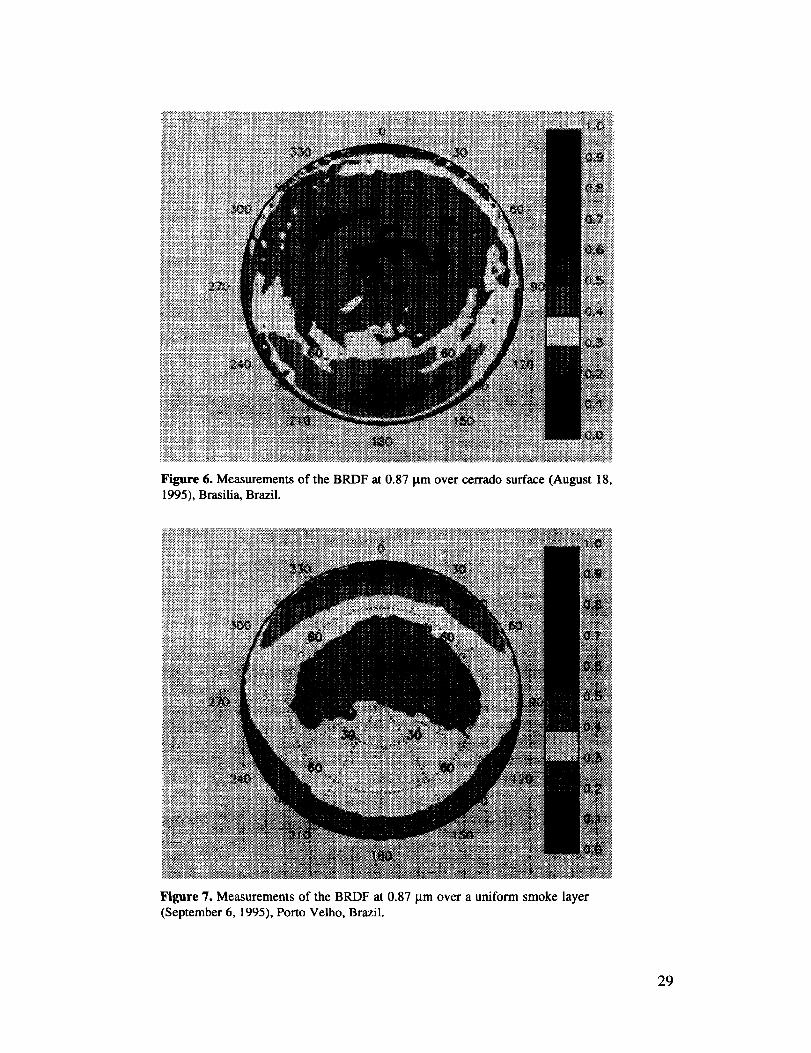
Figure 6. Measurements of the BRDF at 0.87 lxm over cerrado surface (August 18,

1995), Brasilia, Brazil.

Figure 7. Measurements of the BRDF at 0.87 _tm over a uniform smoke layer

(September 6, 1995), Porto Velho, Brazil.

29

Figure 8. Same as in Figure 7 except presented as a 3D surface plot.

6.3 Multi-spectral Imaging

A third use of the CAR inslrurnent is as a downward-looking imager. It supplements

another airborne imaging system, the MODIS Airborne Simulator (MAS). In a downward-

imaging configuration, the CAR is rotated 90 ° around the aircraft's principal axis from its

usual starboard viewing position. The scan mirror scans 190 ° from the starboard horizon,

past the nadir and then the port side horizon. To acquire good quality Earth-view images

and simplify geometric corrections for postflight image processing, the C-131A aircraft

should maintain straight flight track at constant aircraft speed, constant altitude, zero pitch

and roll angle whenever possible.

The CAR imaging capability was first demonstrated on September 4, 1995, during a transit

flight (Flight 1698) from Cuiab_t to Porto Velho, SCAR-Brazil. Figure 9 is a CAR quick-

look image (0.86 Brn) for that historical flight. The horizontal axis denotes the time code

HH:MM in UTC, and the vertical axis is the viewing angle, ranging from 90 ° (the

starboard horizon) to 270 ° (the port side horizon). The airplane travels, on average, 25

meters between the first and the last scan pixels within a CAR active scan, and 48 meters

between scans. To avoid oversampling at nadir, the aircraft's cruising altitude should be

30

below 2750 meters. In the case shown, the average altitude is 4500 meters, corresponding

to an 80-meter footprint at nadir.

270

Cloud Absorption Radiometer Flight 1698

U)

_)

0)t"

<t-

o

GO

225

180

135

90

14:50

270

14:55 14:59 15:03 15:07 15:12 15:16

UTC Time (HH:MM)

90

15:16 15:20 15:25 15:29 15:33 L5:37 15:42

UTC "13me(HH:MM)

Figure 9. CAR 0.86 gm Earth-view image, flight 1698, September 4, 1995, SCAR-B field experiment.

31

7. CAR Contact List

Below is a list of persons involved with the processing and analysis of CAR data.

Dr. Michael King (Principal Investigator)

Code 900, NASA Goddard Space Flight Center

Greenbelt, MD 20771

(301) 286-8228, king@climate.gsfc.nasa.gov

Dr. Si-chee Tsay (Research Scientist)

Code 913, NASA Goddard Space Flight Center

Greenbelt, MD 20771

(301 ) 286-9710, tsay @ climate.g sfc.nasa.gov

Mr. Tom Arnold (CAR Calibration)

Code 913, NASA Goddard Space Flight Center

Greenbelt, MD 20771

(301) 286-4805, arnold@climate.gsfc.nasa.gov

Mr. Jason Li (Data Processing and Analysis)

Code 913, NASA Goddard Space Flight Center

Greenbelt, MD 20771

(301) 286 1029, jyli@climate.gsfc.nasa.gov

Mr. Ward Meyer (Data Processing and Analysis)

Code 913, NASA Goddard Space Flight Center

Greenbelt, MD 20771

(301) 286-4591, meyer @ climate.gsfc.nasa.gov

Dr. Robert Pincus (Research Scientist)

Code 913, NASA Goddard Space Flight Center

Greenbelt, MD 20771

(301) 286-8272, pincus @ climate.gsfc.nasa.gov

Dr. Peter Soulen (Research Scientist)

Code 913, NASA Goddard Space Flight Center

Greenebelt, MD 20771

(301 ) 286-1008, soulen @ climate.gsfc.nasa.gov

32

8. References

King, M. D., 1981: A method for determining the single scattering albedo of clouds

through observation of the internal scattered radiation field. J. Atmos. Sci., 38,2031-2044.

King, M. D., M. G. Strange, P. Leone, and L. R. Blaine, 1986: Multiwavelength

scanning radiometer for airborne measurements of scattered radiation within clouds.

J. Atmos. Oceanic Technol., 3,513-522.King, M. D. (1981). J. Atmos. Sci. 38,2031-2044.

King, M. D., L. F. Radke and P. V. Hobbs, 1990: Determination of the spectral

absorption of solar radiation by marine stratocumulus clouds from airborne

measurements within clouds. J. Atmos. Sci., 47,894-907.

King, M. D., 1992: Directional and spectral reflectance of the Kuwait oil-fire smoke. J.

Geophys. Res., 97, 14545-14549.

King, M. D., L. F. Radke, and P. V. Hobbs, 1993: Optical properties of marine strato-

cumulus clouds modified by ships. J. Geophys. Res., 98, 2729-2739.

King, M. D., 1993: Radiative properties of clouds. Aerosol-Cloud-Climate Interactions,

P. V. Hobbs, Ed., Academic Press, 123-149.

Radke, L. F., J. A. Coakley, Jr., and M. D. King, 1989: Direct and remote sensing

observations of the effects of ships on clouds. Science, 246, 1146-1149.

Nakajima, T., and M. D. King, 1990: Determination of the optical thickness and effective

particle radius of clouds from reflected solar radiation measurements. Part I:

Theory. J. Atmos. Sci., 47, 1878-1893.

Nakajima, T., M. D. King, J. D. Spinhirne, and L. F. Radke, 1991: Determination of the

optical thickness and effective particle radius of clouds from reflected solar radiation

measurements. Part II: Marine stratocumulus observations. J. Atmos. Sci, 48,728-750

Tsay, S.C, M. D. King, and J. Y. Li, 1996: SCAR-B airborne spectral measurements of

surface anisotropy. SCAR-B Science Symposium 96, Fortaleza, Brazil.

33

Appendix A. On-Line Resources

1. CAR Information Server:

This WWW home page located at http : //climate. gs fc.nasa. gov/-jyli/CAR, html.

Click on the navigation bar at the bottom of the main web page, you can obtain:

• a description of the CAR instrument;

• information on field experiments, data distributions, and examples of scientific results;

• programs for reading and visualizing the CAR HDF data;

• a list of references;

• contact information.

Wherever appropriate, links to other relevant web sites are also provided by this primary

CAR information server.

2. Anonymous FTP site:

You may obtain a test CAR HDF data file and sample programs directly from the CAR web

site, or by anonymous FTP to climate, gsfc. nasa. gov, then

login: ftp

password: <your-email-address>

change directory to pub/jyli/CARdownload README file for more detailed information.

34

REPORT DOCUMENTATION PAGE FormApprovedOMB No. 0704-0188

Public reportingburdenfor this collectionof informationis estimated to average 1 hour per response, includingthe time for reviewing instructions,searchingexisting data sources,gathering and maintainingthe data needed, end completing and reviewingthe collection of information. Send comments regardingthis burden estimateor any other aspect of thiscollection of information,includingsuggestionsfor reducingthis burden,1o WashingtonHeadquarters Services, Direclorete for InformationOperations end Reports, 1215 JeffersonDavis Highway, Suite 1204, Arlington,VA 22202-4302, and to the Office of Management and Budget, Paperwork Reduction Project(0704-0188), Washington, DC 20503.

1. AGENCY USE ONLY (Leave blank) 2. REPORT DATE 3. REPORT TYPE AND DATES COVERED

March 1997 Technical Memorandum

4. TITLE AND SUBTITLE 5. FUNDING NUMBERS

The Cloud Absorption Radiometer HDF Data User's Guide

6. AUTHOR(S)

Jason Y. Li, Howard G. Meyer, G. Thomas Arnold, Si-Chee Tsay,

and Michael D. King

7. PERFORMING ORGANIZATION NAME(S) AND ADDRESS (ES)

Goddard Space Flight Center

Greenbelt, Maryland 20771

D. SPONSORING I MONITORING AGENCY NAME(S) AND ADDRESS (ES)

National Aeronautics and Space Administration

Washington, DC 20546-0001

C-1269-25

Code 913

8. PEFORMING ORGANIZATION

REPORT NUMBER

97B00041

10. SPONSORING I MONITORINGAGENCY REPORT NUMBER

NASA TM- 104643

11,. SUPP, I._MENT_RY = NOT]ES ,LIano i-u'noia: .-,pp,eo Research Corporation, Landover, Maryland

Meyer: Science Systems and Applications, Landover, Maryland

Tsa), and Kin_: Goddard Space Flight Center, Greenbelt, Mar),land12a. DISTRIBUTION I AVAILABILITY STATEMENT 12b. DISTRIBUTION CODE

Unclassified - Unlimited

Subject Category 31

Availability: NASA CASI (301) 621-0390.

13. ABSTRACT (Maximum 200 words)

The purpose of this document is to describe the Cloud Absorption Radiometer (CAR) Instrument,

methods used in the CAR Hierarchical Data Format (HDF) data processing, the structure and format of

the CAR HDF data files, and methods for accessing the data. Examples of CAR applications and their

results are also presented.

The CAR instrument is a multiwavelength scanning radiometer that measures the angular distributionsof scattered radiation.

14. SUBJECT TERMS

User's Guide, Cloud Absorption Radiometer, Remote Sensing, Airborne

17. SECURITY CLASSIFICATION

OF REPORT

Unclassified

NSN 7540-01-280-5500

18. SECURITY CLASSIFICATIONOF THIS PAGE

Unclassified

19. SECURITY CLASSIFICATION

OF ABSTRACT

Unclassified

15. NUMBER OF PAGES44

16. PRICE CODE

20. UMITATION OF ABSTRACT

UL

Standard Form 298 (Rev, 2-89)Prescribed by ANSI Std. Z39.18298-102