Embed Size (px)
Citation preview

MA
EGNS
IT A T
MOLEM
UN
IVERSITAS WARWICENSIS
The Classification of Three-dimensional
Lie Algebras
by
Allegra Fowler-Wright
Thesis
Submitted to The University of Warwick
Mathematics Institute
04/2014
CONTENTS
Contents
1 Foundations 1
1.1 Introduction . . . . . . . . . . . . . . . . . . . . . . . . . . . . . . . . . . . 1
1.2 Overview . . . . . . . . . . . . . . . . . . . . . . . . . . . . . . . . . . . . 2
1.3 Preliminaries . . . . . . . . . . . . . . . . . . . . . . . . . . . . . . . . . . 2
2 Lie Algebras of Dimension One and Two 3
3 The First Steps of Classification 4
3.1 Type 1 - The Trivial Lie Algebra . . . . . . . . . . . . . . . . . . . . . . . 5
3.2 Type 2 . . . . . . . . . . . . . . . . . . . . . . . . . . . . . . . . . . . . . . 5
3.3 Type 3 . . . . . . . . . . . . . . . . . . . . . . . . . . . . . . . . . . . . . . 7
3.4 Type 4 - Part I - The Simple Lie Algebras . . . . . . . . . . . . . . . . . . 13
4 Quaternion Algebras 16
4.1 Quaternion Algebras as Quadratic Spaces . . . . . . . . . . . . . . . . . . 18
4.2 Pure Quaternions . . . . . . . . . . . . . . . . . . . . . . . . . . . . . . . . 19
4.3 The Link Between Type 4 and Quaternion Algebras . . . . . . . . . . . . 20
4.4 Wedderburn’s Theorem . . . . . . . . . . . . . . . . . . . . . . . . . . . . 21
4.5 The Brauer Group . . . . . . . . . . . . . . . . . . . . . . . . . . . . . . . 22
5 Type 4 - Part II 27
5.1 Classification Over a Given Field . . . . . . . . . . . . . . . . . . . . . . . 27
5.2 Representations . . . . . . . . . . . . . . . . . . . . . . . . . . . . . . . . . 29
6 Constructing an Invariant Bilinear Form on Simple Three-dimensionalLie Algebras 31
6.1 Setting the Scene . . . . . . . . . . . . . . . . . . . . . . . . . . . . . . . . 31
6.2 Explicit Construction of a Bilinear Form . . . . . . . . . . . . . . . . . . . 33
7 Classification for Fields of Characteristic Two 36
7.1 Type 1 and 2 in Characteristic Two . . . . . . . . . . . . . . . . . . . . . 36
7.2 Type 3 in Characteristic Two . . . . . . . . . . . . . . . . . . . . . . . . . 36
7.3 Type 4 in Characteristic Two - Part I . . . . . . . . . . . . . . . . . . . . 38
7.4 Linear Algebra in Characteristic Two - Symmetric Bilinear Forms . . . . 39
Allegra Fowler-Wright i

CONTENTS
7.5 Examples over Specific Fields . . . . . . . . . . . . . . . . . . . . . . . . . 43
7.6 Type 4 in Characteristic Two - Part II . . . . . . . . . . . . . . . . . . . . 45
7.7 Quaternion Algebras in Characteristic Two . . . . . . . . . . . . . . . . . 47
7.8 Representations of Type 4 Lie algebras . . . . . . . . . . . . . . . . . . . . 48
8 Results 51
A Fields and their Multiplicative Groups 53
A.1 Algebraically Closed Fields . . . . . . . . . . . . . . . . . . . . . . . . . . 53
A.2 The Real Numbers . . . . . . . . . . . . . . . . . . . . . . . . . . . . . . . 53
A.3 Finite Fields . . . . . . . . . . . . . . . . . . . . . . . . . . . . . . . . . . 53
A.4 The Local Field Fq((t)) . . . . . . . . . . . . . . . . . . . . . . . . . . . . 53
A.5 The p-adic Number Fields . . . . . . . . . . . . . . . . . . . . . . . . . . . 54
B Restricted Lie Algebras 56
Allegra Fowler-Wright ii
1 FOUNDATIONS
1 Foundations
1.1 Introduction
Although the term Lie algebra has only been around since 1933 (found in the work of H.Weyl), its concept dates back to 1873 through the work of Sophus Lie. S. Lie wanted toinvestigate all possible local group actions on manifolds and relate it to its ‘infinitesimalgroup’ (its Lie algebra). The importance of Lie algebras then became apparent as ‘local’problems concerning continuous groups of transformations (today known as Lie groups)could be reduced to problems on Lie algebras, which, being linear objects, are moreaccessible to deal with, [1].
It was Wilhelm Killing whom initiated, as a preliminary requirement for the classificationof group actions, the need for classification of finite-dimensional Lie algebras. Between1888 and 1890 Killing produced a series of results concerning the classification of simplecomplex finite-dimensional Lie algebras. However, Killing’s proofs were often incompleteor incorrect and it was E. Cartan who rigourised the results and proofs in his p.H.D thesisin 1894, [2]. Four years later, L. Bianchi managed to classify all three-dimensional realalgebras into eleven classes [3], now famously known as Bianchi classification. His workbeing It should be remarked however, that due to new algorithms, which generalise tohigher dimensions and arbitrary fields, the Bianchi classification is rarely presented bythe original Bianchi method.
Classification theory of finite-dimensional Lie algebras over fields with positive character-istic, p, was initiated later on, in the 1930s by E. Witt, H. Zassenhaus and N. Jacobson,[4]. Since then other pioneers of research have been A. Kostrikin and I. Shafarevich, whoconjectured the isomorphism classes of restricted simple Lie algebras for p > 5, and R.Block and R.Wilson, who were first to prove Kostrikin and Shafarevich’s conjecture forp > 7 [5], [6].
Zassenhaus, together with J. Patera, also classified solvable Lie algebras up to dimensionfour over perfect fields of zero characteristic, [7], [8]. They created a new algorithm,deriving Lie algebras from a list of the isomorphism classes of nilpotent Lie algebras.In 2004 W. De Graaf completed the work done by Zassenhaus and Patera, classifyingthe three and four-dimensional Lie algebras over fields of any characteristic with preciseconditions for isomorphism, [9]. His method uses Grobner bases and a computer algebrasystem, Magma. Unfortunately the method is not known to be able to easily extend tohigher dimensions and thus is not favourable.
This paper will attempt the classification of three-dimensional Lie algebras over bothzero and non-zero characteristic, using a different method than that of De Graaf. Ofcourse by working over an arbitrary field, only being refined by its characteristic, causes arestriction to the detail in which classification can be done. For this reason classificationover certain fixed fields will also be studied. In particular, three-dimensional Lie algebrasshall be classified in detail over C,R,Fpn ,Fpn((t)) and Qp for all p prime and n ∈ N.Details of such fields can be found in Appendix A.
Allegra Fowler-Wright 1

1 FOUNDATIONS
1.2 Overview
This paper consists of three main parts; sections 2 to 5 covers the classification of three-dimensional Lie algebras over fields of zero and odd characteristic, section 6 providesdetails on constructing a special bilinear form on a simple Lie algebra (the importanceof which will become apparent), and section 7 completes the classification of three-dimensional Lie algebras by classifying them over fields of characteristic two. The finalsection, section 8, merely compiles the results found into a tabular overview.
1.3 Preliminaries
Throughout this paper L will denote a finite-dimensional Lie algebra over a field F . F ∗
will be used to denote the non-zero elements in F .
The reader is expected to have a basic background knowledge of the theory of Liealgebra’s as well as being at ease with advanced linear algebra. For the less experiencedreader Chapters 1 to 4 in K. Erdamann and M. Wildon’s book [10], provides a goodfoundation to the theory of Lie algebras whilst Howard Anton’s book [11], Chapters 1,2 and 7, provides a sufficient background in linear algebra.
In classification of three-dimensional Lie algebras, the following isomorphism invariantproperties shall be identified:
(1) The dimension and nature of the derived algebra L′, where L′ := [L,L].
(2) Solvability of L, where L(1) = L′ and ∀n ∈ N>1, L(n) := [L(n−1), L(n−1)].
(3) Nilpotency of L, where L0 = L and ∀n ∈ N, Ln := [Ln−1, L].
(3) The dimension and identification of the radical of L, that is the largest solvable idealof L, denoted by R(L).
(4) The dimension and identification of the centre of L, that is the set:
Z(L) := {x ∈ L : [x, y] = 0 ∀y ∈ L}
(5) The restrictability of L when the characteristic of F is non zero. Restrictability is aproperty of Lie algebras and a brief introduction to the subject is given in Appendix B.
Explicit examples of Lie algebras will often be given in order to substantiate the clas-sification theory as well as the correspondance to the Bianchi classification in the realcase.
Frequently a given associative algebra A, will be used to form a Lie algebra, denotedby A(−).This is an algebra with the same elements as A and addition as in A, but withthe Lie product: [x, y] := x · y − y · x for x, y ∈ A and where x · y is multiplication inA. Of particular interest will be the Lie algebra Mn(F )(−) where Mn(F ) denotes theF -algebra of n× n matrices, with its identity matrix denoted by In.
Allegra Fowler-Wright 2

2 LIE ALGEBRAS OF DIMENSION ONE AND TWO
The adjoint mapping will also continually play a part in classification and thus its defini-tion is important to clarify; In this paper the notation adx, for x ∈ L, will be given to themap L → L defined by adx(y) = [y, x], ∀y ∈ L. The Killing form on L is subsequentlydefined as the map:
< ·, · >: L× L→ F < x, y >:= Tr(adx · ady)
2 Lie Algebras of Dimension One and Two
For the purpose of later reference only, this section will classify Lie algebras of dimensionless than three.
Dimension One
Clearly one must have L = Fx for some x ∈ L where [x, x] = 0. It thus follows that∀y, z ∈ L, as y = αx and z = βx:
[y, z] = [αx, βx] = αβ[x, x] = 0
Thus L is an abelian and clearly unique up to isomorphism.
Example: L = F (−)
Dimension Two
Now L = Fx+ Fy for some linearly independent x, y ∈ L where [x, x] = [y, y] = 0. It isthus only the product [x, y] which needs to be considered:
(a) If [x, y] = 0 then L is abelian.
(b) If [x, y] 6= 0 then define z := [x, y] = αx + βy, where α, β ∈ F are not both zero.With out loss of generality it can be assumed that α 6= 0 and so it follows that [w, z] = zwhere w := α−1y and hence L = Fw + Fz is a Lie algebra such that L′ = Fz. Byconstruction it is clear that this is the only non-abelian two-dimensional Lie algebra upto isomorphism.
The two-dimensional Lie algebra of type (b) will be of particular interest later on and forthis reason shall be given the denotation L2 and shall be studied in a little more detailthrough the following two propositions which can be found, in a more general setting,in Jacobson’s Lie Algebras book, [12], pp10-11.
Definition 1 A derivation, D, is called inner if there exists an x ∈ L such that D = adx
Proposition 2.1 All derivations of L2 are inner.
Proof: Let x, y be a basis for L2 such that [x, y] = x. Since L′2 = Fx is an ideal of L2,for any derivation, D of L2, DL′2 ⊆ L′2. In particular there exists α ∈ F ∗ such thatD(x) = αx. Let E = adαy −D then, E is a derivation so:
[E(x), y] + [x,E(y)] = E([x, y]) = E(x)
Allegra Fowler-Wright 3

3 THE FIRST STEPS OF CLASSIFICATION
But, E(x) = adαy(x) − D(x) = 0, and so it follows that [x,E(y)] = 0 and henceE(y) = βx, for some β ∈ F . Observing that ad−βx is also such that ad−βx(x) = 0 andad−βx(y) = βx, one derives that E = ad−βx and so:
D = adαy − ad−βx = adαy−βx
i.e D is inner. �
Notation: The symbol E will be used to denote the ideal relation between two alegbras,whilst ⊕ will be used to symbolise the direct sum of algebras.
Proposition 2.2 If L is a Lie algebra such that L2 E L, then there exists M E L suchthat L = L2 ⊕M . Moreover, M = ZL(L2), where:
ZL(L2) := {x ∈ L : [x, y] = 0,∀y ∈ L2}
Proof: First it will be proved that ZL(L2) is an ideal in L.
If m ∈ ZL(L2) and l ∈ L then, [l,m] = 0 and by the Jacobi identity, ∀a ∈ L2:
[a[m, l]] = −[m[a, l]]− [a[l,m]]
= −[m[a, l]] (1)
But as L2 E L, one has [a, l] ∈ L2 and so [m, [a, l]] = 0 also. Thus from (1), [a[m, l]] = 0proving that [m, l] ∈ ZL(L2) and hence ZL(L2)E L.
Now it will be proved that L = L2 ⊕ ZL(L2).
If l ∈ L then as L2 is an ideal of L, adl maps L2 into itself, inducing a derivation of L2.By proposition 2.1 this derivation will be inner and so adl |L2= adk for some k ∈ L2.But then this implies [x, l] = [x, k] for every x ∈ L2 and so l − k ∈ ZL(L2). Hence,l = k +m where k ∈ L2 and m := l − k ∈ ZL(L2) which shows that L = L2 + ZL(L2).
Finally L2 ∩ ZL(L2) = ZL2(L2) and ZL2(L2) = 0 so L = L2 ⊕ ZL(L2) as required. �
3 The First Steps of Classification
For any finite-dimensional Lie algebra it’s multiplication, and hence structure, is uniquelydetermined by its structure constants. Explicitly if{e1, e2, ....en} is a basis for L then the structure constants of L are the scalars αkij ∈ Fwhere i, j, k = 1, ...n and [ei, ej ] =
∑nk=1 α
kijek. Thus in the three-dimensional case there
are twenty-seven structure constants to determine. Fortunately, anti-commutativitygives that, for i, j fixed and k = 1, 2, 3, αkii = 0 and that αkij = −αkji. Thus the entireidentification of L lies in just three Lie algebra products and nine possible constants:
[e1, e2] = α112e1 + α2
12e2 + α312e3
[e1, e3] = α113e1 + α2
13e2 + α313e3
[e2, e3] = α123e1 + α2
23e2 + α323e3
Allegra Fowler-Wright 4
3 THE FIRST STEPS OF CLASSIFICATION
In this paper x, y, z will be used to denote a basis, hence it is the products [x, y], [x, z] and[y, z] which will be of interest. Furthermore by bi-linearity of the Lie product, to checkthe Jacobi identity holds, one only needs to check it holds for x, y, z and by permutingthe three basis vectors, this reduces again to simply needing to check the equality:
[[x, y]z] + [[y, z]x] + [[z, x]y] = 0
Classification will begin by using L′ as a tool to derive information about the possibleexistence and uniqueness (up to isomorphism) of three-dimensional Lie algebras. Asystematic approach will be adopted starting with the case that the dimension of L′ iszero. However, it will become apparent that this method is limited and thus furthermethods shall be developed in subsequent sections to give a fuller classification.
3.1 Type 1 - The Trivial Lie Algebra
Type 1 is the trivial case, where the dimension of L′ is zero and hence, forL = Fx+ Fy + Fz, Lie multiplication must be defined by:
[x, y] = 0 [x, z] = 0 [y, z] = 0
This clearly gives rise to a well defined Lie algebra which is unique up to isomorphism.
Properties:
• Abelian.
• Solvable and nilpotent, R(L) = Z(L) = L.
• L is restrictable over a field of characteristic p > 2 since ∀u ∈ L, adu = 0 and so(adu)p = 0. It is not however uniquely restrictable as (adu)p = adv for any v ∈ L.
Bianchi Classification: In the Bianchi classification the Type 1 Lie algebra correspondsto the Bianchi type I.
Example: Any three-dimensional commutative and associative algebra, A over F is such
that A(−) is abelian. In fact any three-dimensional F -algebra can be made into a Liealgebra by defining the Lie product to be identically zero.
3.2 Type 2
Type 2 is defined to be the Lie algebra with dimL′ = 1. This is broken down into twocases, L′ ⊆ Z(L) and L′ * Z(L).
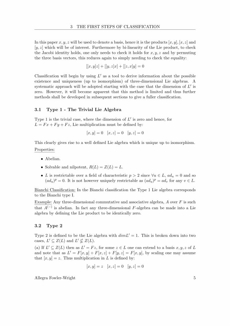
(a) If L′ ⊆ Z(L) then as L′ = Fz, for some z ∈ L one can extend to a basis x, y, z of Land note that as L′ = F [x, y] + F [x, z] + F [y, z] = F [x, y], by scaling one may assumethat [x, y] = z. Thus multiplication in L is defined by:
[x, y] = z [x, z] = 0 [y, z] = 0
Allegra Fowler-Wright 5

3 THE FIRST STEPS OF CLASSIFICATION
It is easily verified that the Jacobi identity holds and consequently L is a well definedLie algebra.
Properties:
• Non-abelian.
• Solvable as L(2) = [L(1), L(1)] = [Fz, Fz] = 0 and thus R(L) = L.
• Nilpotent since L3 = [L′, L] = [Z(L), L] = 0.
• Z(L) = L′.
• Over a field of characteristic p > 2, L is restrictable. This follows from the factLp = 0⇒ ∀u ∈ L, (adu)p = 0 = adz. It is not uniquely restrictable as Z(L) 6= 0.
Remark: This Lie algebra is known as the three-dimensional Heisenberg algebra, namedafter the theoretical physicist, W. Heisenberg. Indeed, it arrises naturally in Physics bythe consideration of the components of the position and momentum vectors of a particleat a given time, to be operators on a Hilbert space, satisfying a specific commutationrelation, see G. Folland, [13], for a more detailed discussion.
Bianchi Classification: In the Bianchi classification the Type 2a Lie algebra correspondsto the Bianchi type II.
Examples: Consider the differential operators, C∞(R3) → C∞(R3), defined by X =
∂x − 12y∂z, Y = ∂y − 1
2x∂z and Z = ∂z. Then X,Y, Z is a representation of theHeinsberg algebra with corresponding Lie algebra bracket,[f, g] = f ◦ g − g ◦ f, ∀f, g ∈ span{X,Y, Z}.Another representation of the Heinsberg Lie algebra is the sub-algebra of strictly upper-triangular matrices in M3(F ). A basis being:
x =
0 1 00 0 00 0 0
y =
0 0 00 0 10 0 0
z =
0 0 10 0 00 0 0
Where one can verify that the only non-zero product is [x, y] = z.
(b) If L′ * Z(L) then L′ = Fx and there exists a y ∈ L such that [x, y] 6= 0. Moreoveras [x, y] ⊆ L′ ⇒ [x, y] = αx for some α ∈ F ∗.Through considering the subalgebra Fx+ Fy in L, one recognises it as the two dimen-sional, non-abelian algebra, L2 and thus by proposition 2.2 L = L2 ⊕ZL(L2). Choosingany z ∈ ZL(L2), gives rise to a basis x, y, z of L such that:
[x, y] = x [x, z] = 0 [y, z] = 0
The Jacobi identity for such a basis is easily verifiable and since L is is completelydetermined by L2, uniqueness follows.
Properties:
Allegra Fowler-Wright 6

3 THE FIRST STEPS OF CLASSIFICATION
• Non-abelian.
• Solvable as L(2) = [L(1), L(1)] = [Fx, Fx] = 0 and so R(L) = L.
• Not nilpotent since by induction one can show Ln = Fx 6= 0, ∀n ∈ N.
• Z(L) = Fz is one-dimensional.
• L′ = Fx.
• L is restrictable if the characteristic of F is p > 2. Indeed,
adx =
0 0 01 0 00 0 0
ady =
1 0 00 0 00 0 0
adz = 0
And one can compute that (adx)p = 0, (ady)p = ady, (adz)
p = 0. Thus it followsthat L is restrictable but not uniquely since Z(L) 6= 0.
Bianchi Classification: In the Bianchi classification the Type 2b Lie algebra correspondsto the Bianchi type III.
Example: The subalgebra of upper-triangular matrices in M2(F )(−) with basis:
x =
(0 10 0
)y =
(−1 00 0
)z =
(1 00 1
)Forms a Lie algebra of Type 2b as the only non-zero product is [x, y] = x.
3.3 Type 3
Type 3 is defined to be the case when dimL′ = 2. Considering L′ as a Lie algebra inits own right, it follows from section 2 that it must be either abelian or L2. HoweverL′ 6= L2. To see this assume, for a contradiction, that L′ = L2 then by proposition2.2 L = L2 ⊕ ZL(L2) and it follows that L′ = L′2 ⊕ ZL(L2)′ ∼= L′2. But L′ = L2 andL′ ∼= L2 implies L2
∼= L′2, absurd since L′2 is one-dimensional. Therefore L′ is the abeliantwo-dimensional Lie algebra.
Choose a basis x, y of L′ and extend it to a basis x, y, z of L, then, there will exista, b, c, d ∈ F , such that:
[x, y] = 0 [x, z] = ax+ by [y, z] = cx+ dy
Where one of a, b and one of c, d can not equal zero. Now as:
[[x, y]z] + [[y, z]x] + [[z, x]y] = [0, z] + [cx+ dy, x] + [−ax− by, y] = 0
Allegra Fowler-Wright 7

3 THE FIRST STEPS OF CLASSIFICATION
the Jacobi identify holds and imposes no further conditions on a, b, c or d. It is thus notimmediately obvious how it can be determined when two Lie algebras of this type areisomorphic as a, b, c, d ∈ F have little restrictions on them.
Thus in order to examine isomorphism classes of this type, the problem is tackled directlyby trying to build an isomorphism and observing what happens. So assume that L andL are two Lie algebras of Type 3 that are isomorphic. Let x, y, z be a basis of L withstructure constants as above, and x, y, z be a basis of L such that L′ = Fx + F y. Letφ : L → L be an isomorphism between the two Lie algebras. Since φ will restrict to anisomorphism between L′ and L′, it follows that φ(z) = αz + w for some α ∈ F ∗ andw ∈ L. Thus for any v ∈ L′,
[φ(v), φ(z)] = φ([v, z]) = φ ◦ adz(v)
But also:[φ(v), φ(z)] = [φ(v), αz + w] = α(adz ◦ φ)(v)
Thus φ ◦ adz = α(adz ◦ φ) = adαz ◦ φ. This informs that if the two Lie algebras areisomorphic, then the linear maps adz and adαz are necessarily similar.
Remark: For L = Fx+ Fy+ Fz such that L′ = F [x, z] + F [y, z], the map adz : L′ → L′
is an isomorphism and so the matrix of adz will be non-singular.
Essentially the above results imply that classification of Type 3 Lie algebras boils downto the classification of multiplicatively similar, non-singular, 2× 2 matrices over F andit is this classification which shall now be attempted. As, over an arbitrary field, theexistence of the Jordan canonical form of a matrix is not guaranteed, one must look at adifferent, more general canonical form, the rational canonical form, in order to attemptsuch classification.
Definition 2 [14] For a monic polynomial f(x) = xn+an−1xn−1 + ...+a0 where ai ∈ F ,
the companion matrix of f , denoted C(f), is defined to be the n× n matrix:
C(f) :=
0 0 . . . 0 −a0
1 0 . . . 0 −a1
0 1 . . . 0 −a2...
.... . .
......
0 0 . . . 1 −an−1
Theorem 3.1 Let M ∈ Mn(F ). Then M is similar over F to a unique block-diagonalmatrix containing the blocks C(p1), ..., C(ps) where C(pk) is the companion matrix of anon-constant monic polynomial pk, and pk|pk+1 for 1 ≤ k ≤ s− 1.
The unique block-diagonal matrix is called the rational canonical form of M and thepolynomials pi are the invariant factors of M . For a proof and further discussion see C.MacDuffee, [14].
Allegra Fowler-Wright 8

3 THE FIRST STEPS OF CLASSIFICATION
It is thus clear that the possible rational canonical forms of M ∈M2(F ), M non-singular,are:
A1 :=
(a 00 a
)A2 :=
(0 a1 0
)A3 :=
(0 a1 b
)where a, b ∈ F ∗.Thus, returning to the lie algebra L, through scaling the basis elements y and z, it canbe assumed that the basis x, y, z of L is such that adz is described by one of the modifiedforms of A1, A2 and A3:
A1 :=
(1 00 1
)A2,c :=
(0 c1 0
)A3,d :=
(0 d1 1
)And so the possible characteristic polynomial, χ(X), of adz are:
A1 - χ(X) has two repeated roots in F , χ(X) = (X − 1)2
A2,c - χ(X) has two roots with zero sum, χ(X) = X2 − cA3,d - χ(X) has two roots with non-zero sum, χ(X) = X2 −X − dWhere c, d ∈ F ∗. These possible matrices of adz give rise to the possible Lie productsof a Type 3 Lie algebra:
Type A1
[x, y] = 0 [x, z] = x [y, z] = y
Type A2,c
[x, y] = 0 [x, z] = cy [y, z] = x
Type A3,d
[x, y] = 0 [x, z] = dy [y, z] = x+ y
The Lie algebras with multiplication defined as above will be denoted L1, L2,c and L3,d
respectively.
So the question arises as to whether L1, L2,c and L3,d are isomorphic for any c, d ∈ F ∗.Furthermore is it possible to have L2,c
∼= L2,e and L2,d∼= L2,f for c 6= e ∈ F ∗ and
d 6= f ∈ F ∗?To answer these questions, previous discussion is recalled, that an isomorphism existsbetween two Type 3 Lie algebras: L = Fz i L′ and L = F z i L′ if, and only if, thematrix A of adz |L′ is similar to the matrix αB of adαz |L′ where now the assumption thatboth A and B are in modified rational canonical form is made. i.e A ∈ {A1, A2,c, A3,d}and B ∈ {A1, A2,e, A3,f} where c, d, e, f ∈ F ∗. Clearly a necessary condition is that therespective possible characteristic polynomials of A:
(X − 1)2, X2 − c, X2 −X − d
Allegra Fowler-Wright 9

3 THE FIRST STEPS OF CLASSIFICATION
matches that of αB:
(X − α)2, X2 − α2e, X2 − αX − α2f
From observation it is clear that only characteristic polynomials from the same type ofrational canonical form can be equivalent, so L1, L2,· and L3,· form three non-isomorphicfamilies of Type 3 Lie algebras. In addition, by comparing coefficients of the character-istic polynomials, one sees that:
• If A = A1 and B = A1 then α = 1.
• If A = A2,c and B = A2,e ⇔ c = α2e or c = e, with the ‘only if’ derived by
calculating that PAP−1 = αB where P :=
(0 cα−1
1 0
).
• If A = A3,d and B = A3,f ⇔ α = 1 and d = f
Thus for every field F there are the following families of non-isomorphic Type 3 Liealgebras:
• L1
• L2,c for c ∈ F ∗. Individual members of this family isomorphism type depends onlyon the square class of c. Thus there are |F× : F×2| in the family.
• L3,d for d ∈ F ∗ and there are |F ∗| non-isomorphic members in this family.
Examples: The following examples make use of knowledge of the multiplicative groupsof the given fields. Appendix A provides the details of such groups.
1. Over any algebraically closed field, K, K∗ = (K∗)2 so ∀a, e ∈ K, ∃α =√
ce ∈ K
such that c = α2e. Thus the non-isomorphic Lie algebras of Type 3 are L1, L2,1
and the family L3,d for d ∈ K∗.
2. Over R one can correspond the Type 3 classification with the traditional Bianchiclassification. Indeed type L1 corresponds to type V in the Bianchi classification.Then, as there are only two square classes in R, there are only two membersin our second family, namely L2,1 which corresponds to type VI0 in the Bianchiclassification and L2,−1 which corresponds to type VII0. Finally the family L3,·corresponds to types IV, VI and VII. As is seen, the advantage of working overR is that further division of the family L3 can be done through considering thepossible eigenvalues of the adjoint matrices.
3. Over a finite field, Fq, where q = pn for some n ∈ N. As Fq has two square classes,with representations 1 and u for some u ∈ F∗q , one can explicitly count the numberof Type 3 Lie algebras, there are:
L1 L2,1 L2,u L3,d
Allegra Fowler-Wright 10

3 THE FIRST STEPS OF CLASSIFICATION
Where d ranges from 1 to q − 1. This gives a total of q + 2 non-isomorphic Liealgebras of Type 3.
4. Over Fq((t)) there are four square classes with representations 1, u, t, ut where 1and u represent the two square classes in Fq. Thus there are the five pairwisenon-isomorphic Lie algebras:
L1 L2,1 L2,u L2,t L2,ut
Together with the infinite family of Lie algebras L3,d, d ∈ Fq((t))∗.
5. Over Qp, p 6= 2, there are four square classes with representations 1, w, w,wpwhere w is a p − 1 root of unity. Thus there are the five distinct non-isomorphicLie algebras:
L1 L2,1 L2,w L2,p L2,wp
And the infinite family of Lie algebras L3,d, d ∈ Q∗p.
6. Over Q2, there are eight square classes with representations 1, 2, 3, 5, 6, 7, 10, 14,thus there are nine distinct distinct non-isomorphic Lie algebras:
L1 L2,1 L2,2 L2,3 L2,5 L2,6 L2,7 L2,10 L2,14
And the infinite family of Lie algebras L3,d, d ∈ Q∗2.
The above classification is verified by De Graaf’s ([9]) findings as well as that of Strade([15]) who tackles the classification of Type 3 Lie algebras directly for the finite case in
Proposition 3.1. Though one must note that Strade includes the matrix
(1 00 −1
)in
his classification, which is not in rational canonical form. However, through the change
of basis matrix on L′,
(1 −1
21 1
2
), the action of z in this new basis of L′ is in rational
canonical form, and one sees that it describes the Lie algebra L2,1.
General properties of a Type 3 Lie Algebra, L with basis x, y, z andL′ = Fx+ Fy:
• Non-abelian.
• Solvable since L(2) = [L′, L′] = 0 and thus R(L) = L.
• Not nilpotent as by induction one shows that Ln = L′ 6= 0, ∀n ∈ N.
• Z(L) = 0 since if v ∈ Z(L) then, in particular, adz(v) = [v, z] = 0 and as adz |L′is an isomorphism it follows that v = βz for some β ∈ F . But then βadz(x) =[x, v] = 0 which is only possible if β = 0 and hence v = 0. Thus Z(L) = 0.
• L′ = Fx+ Fy is abelian (as seen at the start).
Allegra Fowler-Wright 11

3 THE FIRST STEPS OF CLASSIFICATION
• If the characteristic of F is p > 2 then L is a restrictable Lie algebra if, and only if,it is of type L1. Indeed, for L1, (adx)p = 0, (ady)
p = 0 and (adz)p = adz. However,
L2,c is such that:
(adz)p =
cp−1 0 00 cp−1 00 0 0
And so if there was a u ∈ L such that adu = (adz)
p then x, y, z, where z := 1cp−1u,
are such that:[x, y] = 0 [x, z] = x [y, z] = y
Indicating that the change of basis z → z defines an isomorphism between L1 andL2,c, which is impossible. So no such u exists and L2,c is not restrictable.
Similarly, in L3,d, (adz)p gives rise to a matrix representation which cannot repre-
sent adu for any u ∈ L3,d and thus is not restrictable.
Bianchi Classification: In the Bianchi classification the Type 3 Lie algebras correspondto the Bianchi types IV, V, VI, VI0, VII and VII0, as already discussed.
Example:
Definition 3 The generalised orthogonal group O(n; k), is the subgroup of Gl(n+ k;R)which preserves the bilinear form on Rn+k:
[x, y]n,k := x1y1 + ...+ xnyn − xn+1yn+1 + ...+ xkyk
Definition 4 Let n ∈ N≥1. The Poincaire group P (n; 1), is defined as the group oftransformations on Rn of the form T = TxA, where A ∈ O(n − 1; 1) and Tx is thetranslation map on Rn sending y 7→ y + x.
The Poincaire group P (2; 1), is isomorphic to the group of 3× 3 matrices of the form:(A x0 1
)Where A ∈ O(1, 1) and x ∈ R2. As P (2; 1) is a matrix Lie group ([16], Chapter 1),one can associate to it a Lie algebra L with elements X ∈ M3(R) such that exp(tX) ∈P (2; 1),∀t ∈ R.
The resulting associated Lie algebra has basis:
x =
0 0 10 0 −10 0 0
y =
0 0 10 0 10 0 0
z =
0 1 01 0 00 0 0
Such calculations are stimulated through properties of the the matrix exponential map,namely X = d
dtetX |t=0 and det(etX) = eTrX . Such properties can be found in B. Hall,
Allegra Fowler-Wright 12

3 THE FIRST STEPS OF CLASSIFICATION
[16], Chapter 2. Hall also provides the computations needed for determining the Eu-clidean Lie algebra from its Lie group, which provides an analogue for the computationsneeded to calculate the above, (p42-43).
Remark: The resulting Lie algebra represented above has multiplication defined by:
[x, y] = 0 [x, z] = x [y, z] = −y
And this is not in canonical form. However, by noting that adz has characteristic poly-
nomial x2 − 1, one knows it should have rational canonical form:
(0 11 0
)and hence
it is the Lie algebra L2,1. Indeed, by changing the basis of L to x− y, x+ y, z, one findsthat:
[x− y, x+ y] = 0 [x− y, z] = x+ y [x+ y, z] = x− yOr more clearly written with x := x− y, y := x+ y, z := z:
[x, y] = 0 [x, z] = y [y, z] = x
3.4 Type 4 - Part I - The Simple Lie Algebras
The final type of three-dimensional Lie algebras to consider is whendimL′ = 3, such an algebra shall be referred to as a Lie algebra of Type 4.
The following is in line will the first few pages of P. Malcolmson’s paper: EnvelopingAlgebras of Simple Three-Dimensional Lie Algebras [17].
If dimL′ = 3 then clearly L = L′ and the usual trick of identifying L′ with an alreadyclassified Lie algebra does not work. However from the fact L = L′ one does gain theknowledge that if x, y, z forms a basis for L then [x, y], [x, z], [y, z] will form a basis also.In particular the change of basis matrix from [y, z], [z, x], [x, y] to x, y, z will be non-singular. Such a change of basis matrix shall be called a structure matrix and denotedby Mx,y,z. The hope is now to characterise L by studying how the structure of L changeswhen moving from a basis of L to that of L′.
So assume there is an isomorphism between two Lie algebras of Type 4, φ : L→ L, thegoal is to find a relation, if any, between L and L’s structure matrices. So let x, y, z bea basis of L and x, y, z be a basis of L. As φ(x), φ(y), φ(z) also forms a basis for L, onecan write: φ(x) = ax+ by+ cz, φ(y) = dx+ ey+ fz and φ(z) = gx+hy+ iz. This givesrise to the change of basis matrix:
A :=
a b cd e fg h i
Through direct calculation, one finds that the change of basis matrix, [φ(y), φ(z)],[φ(z), φ(x)], [φ(x), φ(y)] to [y, z], [z, x], [x, y] is:
P =
ei− fh hc− ib bf − cefg − di ia− gc cd− afdh− ge gb− ha ae− bd
Allegra Fowler-Wright 13
3 THE FIRST STEPS OF CLASSIFICATION
One can then calculate that:
ATP =
det(A) 0 00 det(A) 00 0 det(A)
Thus:
ATP = det(A)I
P = det(A)A−T I
PMx,y,z = det(A)A−TMx,y,z
PMx,y,zA−1 = det(A)A−TMx,y,zA
−1 (2)
Since PMx,y,zA−1 describes a change of basis from [φ(y), φ(z)], [φ(z), φ(x)], [φ(x), φ(y)]
to φ(x), φ(y), φ(z), it is the structure matrix of φ(x), φ(y), φ(z) and so is denoted byMφ(x),φ(y),φ(z). Thus (2) becomes:
Mφ(x),φ(y),φ(z) = det(A)A−TMx,y,zA−1 (3)
Where A describes the isomorphism φ : L → L. This shows that two Lie algebras, Land L, of Type 4 are isomorphic if, and only if, ∃A ∈M3(F ), A non-singular, such that(3) holds.
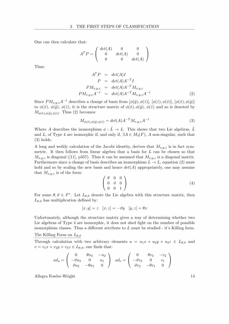
A long and weildy calculation of the Jacobi identity, derives that Mx,y,z is in fact sym-metric. It then follows from linear algebra that a basis for L can be chosen so thatMx,y,z is diagonal ([11], p357). Thus it can be assumed that Mx,y,z is a diagonal matrix.Furthermore since a change of basis describes an isomorphism L→ L, equation (2) musthold and so by scaling the new basis and hence det(A) appropriately, one may assumethat Mx,y,z is of the form: θ 0 0
0 ϑ 00 0 1
(4)
For some θ, ϑ ∈ F ∗. Let Lθ,ϑ denote the Lie algebra with this structure matrix, thenLθ,ϑ has multiplication defined by:
[x, y] = z [x, z] = −ϑy [y, z] = θx
Unfortunately, although the structure matrix gives a way of determining whether twoLie algebras of Type 4 are isomorphic, it does not shed light on the number of possibleisomorphism classes. Thus a different attribute to L must be studied - it’s Killing form.
The Killing Form on Lθ,ϑ
Through calculation with two arbitrary elements u = u1x + u2y + u3z ∈ Lθ,ϑ andv = v1x+ v2y + v3z ∈ Lθ,ϑ, one finds that:
adu =
0 θu3 −u2
−ϑu3 0 u1
ϑu2 −θu1 0
adv =
0 θv3 −v2
−ϑv3 0 v1
ϑv2 −θv1 0
Allegra Fowler-Wright 14

3 THE FIRST STEPS OF CLASSIFICATION
and so:
adu · adv =
−θϑu3v3 − ϑu2v2 θu2v1 θu3v1
ϑu1v2 −θϑu3v3 − θu1v1 ϑu3v2
ϑθu1v3 θϑu2v3 −ϑu2v2 − θu1v1
Thus:
< u, v > = Tr(adu · adv)= −θϑu3v3 − ϑu2v2u3v3 − θu1v1 − ϑu2v2 − θu1v1
= −2(θu1v1 + ϑu2v2 + θϑu3v3)
= uT
−2θ 0 00 −2ϑ 00 0 −2θϑ
v
Hence the Killing form for Lθ,ϑ has a diagonal matrix representation. Furthermore thismatrix representation can be scaled so that it has θ, ϑ and θϑ down the diagonal. Thisshall be called the modified Killing form of Lθ,ϑ and denoted by < θ, ϑ, θϑ >, which isin line with standard notation of quadratic theory, [18], p9.
This leads to the following theorem:
Theorem 3.2 [17] For scalars α, β, θ, ϑ,∈ F ∗, the following are equivalent:
(a) The forms < α, β, αβ > and < θ, ϑ, θϑ > are isometric.
(b) The Lie algebras Lα,β and Lθ,ϑ are isomorphic.
Remark: The notation D(a, b, c) for the diagonal matrix with a, b, c as its diagonal entriesshall be adopted.
Proof: (a) ⇒ (b) Assume that the two forms are isometric. An isometry betweenquadratic forms is equivalent to there being a congruence between their correspondingmatrices. Therefore there exists a non-singular matrix R such that:
D(α, β, αβ) = RD(θ, ϑ, θϑ)RT (5)
Inverting both sides:
D(1
α,
1
β,
1
αβ) = R−TD(
1
θ,
1
ϑ,
1
θϑ)R−1
and multiplying through by αβθϑ :
D(α, β, 1) =αβ
θϑR−TD(θ, ϑ, 1)R−1
Now D(α, β, 1) and D(θ, ϑ, 1) describe the structure matrices of Lα,β and Lθ,ϑ in unmod-
ified form, and so from (3) R describes an isomorphism iff det(R) = αβθϑ . From (5) it can
Allegra Fowler-Wright 15

4 QUATERNION ALGEBRAS
be deduced that (det(R))2(θϑ)2 = (αβ)2. Thus either det(R) = αβθϑ or det(R) = −αβ
θϑ .In the first case R describes the Lie algebra isomorphism required whilst in the secondcase −R does.
(b) ⇒ (a) If Lα,β and Lθ,ϑ are isomorphic then an isomorphism φ, preserves the Lieproducts i.e φ([x, y]) = [φ(x), φ(y)] ∀x, y ∈ Lα,β. It thus follows that Lα,β and Lθ,ϑ willhave the same adjoint matrices and hence the same Killing forms. �
This theorem is important as it means the classification of Type 4 Lie algebras maybe done through the classification of non-singular quadratic forms. Moreover, in thenext section it will be shown that quadratic forms, of this type, are integrally linkedto quaternion algebras. Thus the theory of quaternion algebras will be developed andlinked with that of quadratic forms, and hence Lie algebras. This link will be establishedin order to achieve the end goal of determining the number of non-isomorphic Type 4Lie algebras over a arbitrary field F , of characteristic not equal to 2. This section isconcluded with a few immediate properties of Type 4 Lie algebras.
Properties:
• Non-abelian.
• L is not solvable or nilpotent as by induction one can show thatL(n) = L and Ln = L for all n ∈ N.
• L is simple. For if ∃M E L such that M 6= 0 and M 6= L. Then either dimM = 1or dimM = 2. In either case M is solvable (deducible from section 2) and sincedim(L/M) = 2 or dim(L/M) = 1 it also follows that L/M is solvable. But then,by a well known lemma ([10], p29), M and L/M solvable implies that L is solvable,contradiction.
• Z(L) = 0 and R(L) = 0. This is because Z(L) E L and as L is not abelian,Z(L) 6= L. Similarly R(L)EL and R(L) 6= L as L is not solvable. So by simplicityof L the results follow.
• If the characteristic of F is p > 2, then L is restrictable since its Killing form isnon-degenerate (see Appendix B, theorem B.1).
Remark: As L is simple Ker(adx) = 0 for all x ∈ L, thus ad : L → Der(L) is amonomorphism. This means that every simple Lie algebra is isomorphic to a linear Liealgebra1
4 Quaternion Algebras
This section has been developed from Chapters 3 and 4 of T. Lam’s book on AlgebraicTheory of Quadratic Forms, [18]. However, Lam contains more depth and detail than is
1A linear Lie algebra is a Lie algebra which is a subalgebra of gl(V ), where V is a vector space.
Allegra Fowler-Wright 16
4 QUATERNION ALGEBRAS
necessary for the primary goal of the classification of three-dimensional Lie algebras andthus only the needed results and seemingly insightful proofs are included in this paper.
Definition 5 Let F be a field of characteristic not equal to two.For a, b ∈ F ∗, define the generalised quaternion algebra over F , denoted by (a, b)F , as thefour-dimensional algebra with basis {1, i, j, ij} and multiplication defined by i2 = a, j2 = band ij = −ji.
Since the classification of quaternion algebras will prove vital for the classification ofthree-dimensional Lie algebras, it will be shown that for each a, b ∈ F ∗, (a, b)F not onlyexists but that its isomorphism class, as an algebra over F , is dependent only on theclasses of a and b in F×/F×2.
Existence
Consider the algebraic closure, F , of F . Pick a, b ∈ F such that a2 = a and b2 = b.Define:
i :=
(−a 00 a
)j :=
(0 b
−b 0
)Then:
ij =
(0 ab
ab 0
)= −ji
It is clear that {I2, i, j, ij} forms a linearly independent set over F and hence over F .Thus the span {I2, i, j, ij} forms a four-dimensional algebra over F with multiplicationdefined by i2 = a, j2 = b and ij = −ji which by definition is the algebra (a, b)F .
Relation with F×/F×2
It is an easy exercise to verify that for x, y ∈ F ∗, φ : (a, b)F → (ax2, by2)F defined byφ(i) = xi, φ(j) = yj and φ(a) = a,∀a ∈ F , is an F -algebra isomorphism. Thus (a, b)Fis isomorphic to (c, d)F for all c, d such that c ∈ aF×2 and d ∈ bF×2. Consequently,defining Quat(F ) to be the set of isomorphism classes of quaternion algebras over F ,the map:
σ : F×/F×2 × F×/F×2 → Quat(F )
sending (a, b) to (a, b)F is well defined and surjective.
Remark: It is not yet clear whether σ is injective. In fact, σ rarely is. For example if 1and u are representations for the square classes in Fq, then (1, 1), (1, u) and (u, u) are alldistinct elements of F×q /F×2
q ×F×q /F×2q but they all map to the same element (−1, 1)F in
Quat(F ) (this will be proven later). So the map σ may give insight into how quaternionalgebras are generated, but does not usually give explicit information about the natureof it’s image.
Allegra Fowler-Wright 17

4 QUATERNION ALGEBRAS
4.1 Quaternion Algebras as Quadratic Spaces
Recalling that a quadratic space is a pair (V, P ) where V is an F -vector space and Pa quadratic map from V to F , it is often desirable to consider a quaternion algebra,(a, b)F , as a quadratic space by constructing a quadratic map on it.
Definition 6 The conjugate, q, of an element, q = α+βi+γj+δij ∈ (a, b)F is definedto be the element q := α− βi− γj − δij ∈ (a, b)F .
Properties of the conjugate include:
(1) ¯p+ q = p+ q
(2) pq = pq
(3) ¯p = p
(4) p = p iff p ∈ FThese are all easily verifiable and thus only the final property shall be proved:
If p = ϑ+ κi+ λj + µij ∈ Q then:
p = p⇔ κi+ λj + µij = −(κi+ λj + µij)⇔ κ = λ = µ = 0⇔ p ∈ F �
Essentially properties (1) and (4) reveal that the conjugate, as a map:(a, b)F → (a, b)F is F -linear whilst property (2) reveals that the map is an anti-automorphismand property (3) shows the map is of period 2. A map with such properties is called ainvolution on (a, b)F .
With the definition of a conjugate at hand the norm form on (a, b)F , can now be definedas the map N : (a, b)F → F , sending q ∈ (a, b)F to N(q) = qq.
The map is well defined onto it’s image since ¯N(q) = q ¯q = qq = N(q) which, by property(4) of the conjugate, implies N(q) ∈ F . Furthermore direct computation shows that ifq = α+ βi+ γj + δij then:
N(q) = α2 − aβ2 − bγ2 + abδ2
Hence N is a quadratic form in four variables, α, β, γ, δ and so the standard notation< 1,−a,−b, ab > for N is given.
The unique symmetric bilinear form associated to the norm form can now be defined bythe standard polarisation identity:
B(x, y) :=1
2(N(x+ y)−N(x)−N(y)) ∀x, y ∈ (a, b)F
One can also define the trace form on (a, b)F as the map Tr : (a, b)F → F , Tr(x) := x+x.And through calculation, one arrives at the relation:
B(x, y) =1
2(xy + yx) =
1
2Tr(xy)
Allegra Fowler-Wright 18

4 QUATERNION ALGEBRAS
Which explicitly shows the proportionality of the two forms.
Notation: Q will now often be used to denote an arbitrary quaternion algebra.
Proposition 4.1 An element q ∈ Q is invertible if and only if N(q) 6= 0.
Proof: (⇒) If q is invertible then ∃q−1 ∈ Q such that qq−1 = 1. Taking the norm ofboth sides of this identity gives: N(qq−1) = N(1) = 1. Since N(qq−1) = N(q)N(q−1),it follows that N(q) 6= 0.
(⇐) If N(q) 6= 0 define q−1 := qN(q) then q−1 ∈ Q and qq−1 = 1 and so q is invertible. �
Definition 7 N is anisotropic as a quadratic form if N(v) = 0 ⇒ v = 0. Conversely,if there exists v 6= 0 such that N(v) = 0 then N is called isotropic.
Theorem 4.2 Q is a division algebra if and only if N is anisotropic.
Proof: A consequence of the proposition 4.1 �
4.2 Pure Quaternions
A subspace of a quaternion algebra, called the space of the pure quaternions, shall nowbe studied. It’s significance will become apparent in the section 4.3.
Definition 8 A quaternion q = α+ βi+ γj + δij ∈ Q is called pure if α = 0.
Notation: The set of pure quaternions will be denoted by Q0.
Remark: Note that if q ∈ Q0 then q = −q.One observes that the subspaceQ0 equipped withB is a non-degenerate three-dimensionalquadratic space over F . It is non-degenerate because if q ∈ Q0 then q = βi+γj+δij andB(q, q) = N(q) = −q2 which equals zero iff q = 0. Moreover, as 2B(x, y) = xy + yx =−xy − yx, it follows that B(x, y) = 0 iff y and x anti-commute, thus {i, j, ij} forms anorthogonal basis in Q0 with respect to B. The fact that for every x ∈ Q0, B(x, 1) = 0shows also that the subspace Q0 is orthogonal to F in Q and hence Q = Q0⊥F .
Clearly Q0 may be characterised as follows:
Q0 = {x ∈ Q : Tr(x · 1) = 0}
Proposition 4.3 Let q ∈ Q be such that q 6= 0. Then q ∈ Q0 if, and only if, q2 ∈ F butq /∈ F . In particular, if φ : Q→ Q′ is an algebra isomorphism, then φ(Q0) = Q′0.
Proof: Done through direct calculation of q2 ([18], Proposition II.1.3) �
Allegra Fowler-Wright 19

4 QUATERNION ALGEBRAS
Proposition 4.4 Let Q = (a, b)F and Q′ = (a′, b′)F . Then Q and Q′ are isomorphic asF-algebras if, and only if, Q and Q′ are isometric as quadratic spaces.
Proof: (⇒) Suppose φ : Q → Q′ is an algebra isomorphism. By writing q ∈ Q in theform q = α+ q0, where α ∈ F and q0 ∈ Q0 it follows thatφ(q) = α+ φ(q0). Furthermore, φ(q0) ∈ Q′0 by proposition 4.3. In particular this meansthat ¯φ(q) = α − φ(q0) but then φ(q) = φ(α − q0) = α − φ(q0) also. Hence ¯φ(q) = φ(q).And so:
N(φ(q)) := φ(q) ¯φ(q) = φ(q)φ(q) = φ(qq) = φ(N(q)) = N(q)
Where the last equality follows from the fact that N(q) ∈ F . So indeed φ is an isometryfrom Q to Q′.
(⇐) By Witt’s cancellation theorem ([18], p15) the quadratic forms for Q and Q′ areisometric if, and only if, the quadratic forms for Q0 and Q′0 are isometric. Thus, if Qand Q′ are isometric, then there is an isometry φ : Q0 → Q′0. In particular, N(φ(i)) =N(i) = −a. But, by definition, N(φ(i)) := φ(i) ¯φ(i) = −φ(i)2 and so it follows thatφ(i)2 = a. Similarly φ(j)2 = b. Furthermore,
0 = B(i, j) = B(φ(i), φ(j)) = (−φ(i)φ(j)− φ(j)φ(i))
And so φ(i)φ(j) = −φ(j)φ(i). Finally, as i, j, ij are orthogonal in Q0, φ(i), φ(j) and φ(ij)are orthogonal in Q′0 and it thus follows that Q′ = Q′0⊥F is isomorphic to Q = Q0⊥F.�The proposition is of importance as it informs that in order to determine whether twoquaternion algebras are isomorphic, one can simply check to see if their norms are iso-metric. For example the quaternion algebras (a, b)F and (b, a)F have isometric quadraticforms, hence (a, b)F ∼= (b, a)F ∀a, b ∈ F ∗.
4.3 The Link Between Type 4 and Quaternion Algebras
With the theory of quaternion algebras sufficiently developed, their link with three-dimensional Lie algebras of Type 4 can now be properly established.
Recall from section 3.4 that, for a Lie algebra of Type 4, a basis could be chosen in sucha way that it’s modified Killing form had representation< θ, ϑ, θϑ >, for some θ, ϑ ∈ F ∗. Now, the pure quaternions, in the quaternion algebra(−θ,−ϑ)F , have been shown to form a three-dimensional quadratic space with non-degenerate norm < θ, ϑ, θϑ > i.e their quadratic form is equal to that of the modifiedKilling form on Lθ,ϑ. An extended version of theorem 3.2 can now be given:
Theorem 4.5 [17] For any α, β, θ, ϑ ∈ F ∗, the following are equivalent:
(a) The forms < α, β, αβ > and < θ, ϑ, θϑ > are isometric;
(b) The Lie algebras Lα,β and Lθ,ϑ are isomorphic;
(c) The quaternion algebras (−α,−β)F and (−θ,−ϑ)F are isomorphic.
Allegra Fowler-Wright 20

4 QUATERNION ALGEBRAS
Proof: (a) ⇔ (b) by theorem 3.2 and (a) ⇔ (c) by proposition 4.4. �
Remark: It does not follow that:
Lθϑ ∼= {x ∈ (−θ,−ϑ)F : Tr(x) = 0}(−)
This is because obtaining the modified Killing form does not always correspond to abasis change in L. However, the Lie algebra formed from the pure quaternion algebra:
Q0 = {q ∈ (−4θ,−4ϑ)F : Tr(q) = 0}(−)
Has multiplication defined by:
[y, z] = 4θx [z, x] = 4ϑy [x, y] = z
Where x := j, y := −i, z := ij. This is, by definition, the Lie algebra L4θ,4ϑ. So there isthe isomorphic relationship:
L4θ4ϑ∼= {q ∈ (−θ,−ϑ)F : Tr(x) = 0}(−)
However it is more instructive to think of the correspondence as in theorem 4.5.
4.4 Wedderburn’s Theorem
Since isomorphism classes of Type 4 Lie algebras are in 1-1 correspondence with quater-nion algebras over F , the aim is now to try and categorise the isomorphism classes ofquaternion algebras. This is done by looking at a bigger class of algebras to which theybelong - the class of central simple algebras over F .
Indeed, a quaternion algebra, Q, has center F . This is shown explicitly by picking anelement, q = α+ βi+ γj + δij, in its center, and considering the equations: 0 = qj − jqand 0 = qi− iq. These give that ij(β + δj) = 0 and (γ + δi)ji = 0 respectively. Thus asN(ij) = −N(ji) 6= 0 both ij and ji are invertible and so it follows that β = γ = δ = 0,as required.
A quaternion algebra is also simple as it has no trivial two-sided ideals ([18], p52). Thusa quaternion algebra is indeed a central simple algebra over F . This allows for the appealto a famous theorem from 1907 by Joseph Wedderburn:
Theorem 4.6 (Wedderburn’s Theorem) Any finite dimensional semi-simple algebra, A,is isomorphic to a direct product of r ∈ N simple algebras of the form Mnk(Dk), wherenk ∈ N and Dk are division algebras over F , k = 1, 2...r. Moreover the number r andthe pairs (nk, Dk) are uniquely determined by A.
An extension of this theorem to semi-simple rings was developed by E. Artin in 1927and this generalisation more frequently appears in the literature being referred to as the‘Wedderburn-Artin’ Theorem. A neat proof of such theorem can be found in T. Lam’sbook on Noncommutative Rings, [19], where Schur’s lemma is used along with basicresults from ring theory. Theorem 4.6 directly gives the corollary:
Allegra Fowler-Wright 21

4 QUATERNION ALGEBRAS
Corollary 4.7 A central simple algebra which is finite dimensional over its center, F ,is isomorphic to an algebra Mn(D), where n ∈ N and D is a division algebra over F .
In consequence, given a quaternion algebra Q, there is an n ∈ N and a division algebra Dsuch that Q is isomorphic to Mn(D). By equating possible dimensions over F : dim(Q) =4 and dim(Mn(D)) = n2dim(D), so there are only two possibilities; either n = 1 anddim(D) = 4 or n = 2 and dim(D) = 1. Thus, either Q ∼= M1(D) ∼= D or Q ∼= M2(F ).
Remark: The terminology that an F -algebra splits if it is isomorphic to a full matrixalgebra shall be adopted. Thus for a quaternion algebra Q, Q splits if Q ∼= M2(F ).
From theorem 4.2, Q is a division algebra if and only if its norm is anisotropic. Moreoversince M2(F ) is not a division algebra2 it follows that Q splits if, and only if, its norm isisotropic.
Proposition 4.8 (−1, 1)F wM2(F )
Proof: ([18], p52) Define the linear map φ : (−1, 1)F →M2(F ) by:
φ(i) :=
(0 1−1 0
), φ(j) :=
(0 11 0
), and ∀a ∈ F φ(a) = aI2
Then φ(i)2 = −I2, φ(j)2 = I2 and φ(ij) =
(1 00 −1
)= −φ(ji), so φ is an algebra
homomorphism and since φ(1), φ(i), φ(j) and φ(ij) are linearly independent and generateM2(F ) as a vector space over F , φ is an algebra isomorphism. �
Corollary 4.9 If F is algebraically closed then every quaternion algebra splits over F .
Proof: Let Q = (a, b)F for some a, b ∈ F ∗, then if F is algebraically closed, the polyno-mials p1(x) := ax2 + 1 and p2(x) := bx2 − 1 have roots in F . Let α ∈ F be a root of p1
and β ∈ F a root of p2, then aα2 ∈ −F×2 and bβ2 ∈ F×2, and so:
Q = (a, b)F w (aα2, bβ2)F = (−1, 1)F wM2(F ) �
4.5 The Brauer Group
So far it has been shown that the number of non-isomorphic Lie algebras over F isequal to the number of non-isomorphic quaternion algebras over F . Furthermore, thesequaternion algebras are isomorphic to either M2(F ) or a division algebra over F . Thisshall now be formalised further by the formation of the Brauer group.
2Indeed M2(F ) has zero divisors for example, if Eij denotes the matrix with 1 in position (i, j) thenE11 is a zero divisor: E11E22 = 0.
Allegra Fowler-Wright 22

4 QUATERNION ALGEBRAS
The Brauer group classifies all central simple algebras (CSAs) over F by a similarityrelation. A group structure on the similarity classes is imposed by the tensor product.This subsection will use basic results concerning tensor products of algebras, four inparticular are:
(1) If A is an F -algebra and m,n ∈ N then A⊗Mn(F ) = Mn(A)
(2) Mn(F )⊗Mm(F ) = Mnm(F )
(3) If A, B are CSAs then A⊗B is a CSA
(4) Mn(F ) is a CSA
All of the above results can be found with proofs in K. Szymiczek’s Bilinear Algebrabook, [20] pp329-332, 377-378.
The first step in creating the Brauer group is to define a similarity relation on CSAs, thisis done as follows: A v B if A⊗Mn(F ) is isomorphic as an F -algebra to B ⊗Mm(F ),for some n,m ∈ N.
This similarity relation is indeed well defined with only transitively not being immedi-ately obvious. Thus suppose A v B and B v C then ∃n,m, p ∈ N such that:
A⊗Mn(F ) ∼= B ⊗Mm(F ) and B ⊗Mp(F ) ∼= C ⊗Mq(F )
Thus, using commutivity and associativity of the tensor product:
A⊗Mnp(F ) ∼= (A⊗Mn(F ))⊗Mp(F )∼= (B ⊗Mm(F ))⊗Mp(F )∼= Mm(F )⊗ (B ⊗Mp(F ))∼= Mm(C)⊗ (C ⊗Mq(F ))∼= C ⊗Mmq(F )
So A v C proving that v is indeed transitive.
By denoting the similarity class of A by [A], a multiplicative operation between twoclasses can now be defined by [A][B] := [A ⊗ B] which is routinely checked to be welldefined, commutative and with the class [F ] = [Mn(F )] acting as an identity element.Moreover, through considering the opposite algebra3 of A; Aop, it can be proven thatA⊗Aop ∼= Mn(F ) for some n ∈ N and so [A][Aop] = [F ] ([18], p72). This motivates thefollowing definition:
Definition 9 The Brauer group of a field F , denoted Br(F ), is the set whose elementsare similarity classes of CSAs, where the similarity relation v is defined as above, andwhose group operation is defined by:
[A][B] := [A⊗B]
3Explicitly the opposite algebra is the algebra with the same elements, and addition operation, as Abut with multiplication, op, defined for all a, b ∈ A by (ab)op := b · a where · is multiplication in A.
Allegra Fowler-Wright 23

4 QUATERNION ALGEBRAS
Through commutativity of the tensor product of algebras, it follows that Br(F ) is infact an abelian group.
One must remark that the isomorphism relation of F -algebras is stronger than thesimilarity relation. Clearly A ∼= B ⇒ A v B but the converse can fail. An obviousexample of failure is when n 6= m then Mn(F ) v Mm(F ) but Mn(F ) is not isomorphicto Mm(F ). However, there is still an underlying importance of the Brauer group, and itssimilarity relation, for the study of central simple algebras. It’s importance is partiallyrevealed in the following proposition:
Proposition 4.10 The elements of Br(F ) are in 1-1 correspondence with the isomor-phism classes of F -central division algebras, D ↔ [D].In particular isomorphically distinct quaternion algebras will have different representa-tions in Br(F ).
Proof: Let D,E be central division algebras over F . Then:
[D] = [E] in Br(F )
⇔ ∃n,m ∈ N such that D ⊗Mn(F ) ∼= E ⊗Mm(F )
⇔ ∃n,m ∈ N such that Mn(D) ∼= Mm(E)
⇔ D ∼= E and n = m
Where the first equivalence is by definition, the second by the property of tensor algebrasand the final equivalence follows from the uniqueness part of Wedderburns Theorem.
Now if Q is a quaternion algebra then either Q ∼= D for some central division algebraD, in which case Q↔ [D], or, Q splits and so Q ∼= M2(F ) and thus Q↔ [F ]. �
It is interesting to note that the similarity classes of quaternion algebras in Br(F )have order either 1 or 2. This is seen by considering the opposite quaternion algebraof Q = (a, b)F . Qop has basis {1, i, j, ij} with multiplication defined by (i2)op = a,(j2)op = b and (ij)op = ji = −ij = −(ji)op. It is thus clear that Qop ∼= Q. Hence inBr(F ): [Q][Q] = [Q][Qop] = [F ] so when Q is not split, Q is an element of order twoin Br(F ). Furthermore, as Br(F ) is abelian the subset of elements of order 1 or 2 willform a subgroup, denote this subgroup by Br2(F ). Then if Q(F ) denotes the subgroupgenerated by the similarity classes of quaternion algebras over F , there is the inclusionrelation:
Q(F ) ⊆ Br2(F ) ⊆ Br(F )
Moreover, if Q(F ) is a finite group, it’s order will be an exponent of 2.
Deeper results do exist about the nature of Br(F ); In 1981 A. Merkurjev proved aconjecture, that every element of Br2(F ) is expressible as a tensor product of quaternionalgebras and thus Q(F ) = Br2(F ). So if A is a CSA of dimension four then it isnecessarily a quaternion algebra. The interested reader may refer to G.Philippe and T.Szamuely, [21], for a proof which is beyond the scope of this paper.
Examples of Br(F ) and Q(F ):
Allegra Fowler-Wright 24

4 QUATERNION ALGEBRAS
1. The field of real numbers - R
• Br(R) ∼= Z/2Z, this is Frobenius theorem from 1877 which classifiesfinite-dimensional, associative division algebras over R as isomorphic to oneof R,C or H := (−1,−1)R, [22] . The main ingredients to the proof are theCayley Hamilton Theorem and the Fundamental Theorem of Algebra.
• Q(R) ∼= Z/2Z. This is as R×/R×2 = {1,−1} and so the possible distinctquarternion algebras are (1, 1)R, (−1, 1)R ∼= M2(R) and (−1,−1)R ∼= H. Butthe quaternion algebra (1, 1)R has an isotropic norm, easily seen byconsidering the element 1 + i thus (1, 1)R ∼= M2(R), leaving only M2(R) andH as distinct quaternion algebras.
2. An algebraically closed field - K
• Br(K) = 0. This is as, if D is a finite-dimensional division algebra over K,then for x ∈ D, the minimal polynomial of x is linear since it is irreducibleand F is algebraically closed. Hence K[x] = K. Thus ∀x ∈ D,x ∈ K also⇒ D = K, and so by Wedderburn’s theorem, any finite-dimensional CSA isof the form Mn(K) and hence Br(K) is trivial.
• Clearly Q(K) = 0 and so the only quaternion algebra, up to isomorphismover K is (−1, 1)K . This could also be derived from the observation that,for any a, b ∈ K∗, the norm form of the quaternion (a, b)K , will always beisotropic: N(
√a+ i) = 0.
3. A function field of an algebraic curve over an algebraically closed field - K
• Br(K) = 0. This result is courtesy of Tsen’s theorem ([23], pp116-117)which states that a function field, K, of an algebraic curve over analgebraically closed field is such that every non-constant homogeneouspolynomial f of degree d with k > d variables, over F , has a non-trivialzero. In other words it is quasi-algebraically closed. Br(K) = 0 then followsbecause if there existed a non-trivial CSA of degree n over F , then onecould define a non-degenerate norm on it which is a polynomial of degree nin n2 variables, contradicting Tsen’s theorem.
• Q(K) = 0 so (a, b)K ∼= M2(K) ∀a, b ∈ K∗.• Remark: Algebraic closure of K is vital here. For example it can be shown
that there are uncountably many isomorphism classes of quaternion algebrasover the function field R(t) ([20], p362).
4. A finite field - Fq (q = pn, p > 2)
• Br(Fq) = 0. This is a consequence of Wedderburn’s Little Theroem from1905 ([23], p175) that states any division algebra, and hence domain, D,over Fq is a field. Thus D has center D, meaning that D is a CSA over Fq ifand only if D = Fq.
Allegra Fowler-Wright 25

4 QUATERNION ALGEBRAS
• Q(Fq) = 0 and so ∀a, b ∈ F∗q , (a, b)Fq∼= M2(Fq).
5. The local field Fq((t)), (q = pn, p > 2)
• Br(Fq((t))) ∼= Q/Z. This result is from class field theory, see Chapter 21 inLorenz, [23], for a discussion and a proof.
• Q(Fq((t))) ∼= Z/2Z. This can be seen by considering the elements of ordertwo in Q/Z. It also follows from the discovery that < 1,−u,−t, ut > is, upto isomorphism, a unique anisotropic four-variable quadratic form, overFq((t)), where 1, u, t, ut represent the four square classes of Fq((t)). Henceby theorem 4.5, (u, t)Fq((t)) represents the only isomorphism class ofnon-split quaternion algebras.
The proof of this, for q odd, can be constructed from the material inChapter VI of T. Lam, [18], using proposition 1.9 together with theorem 2.2.
6. The p-adic numbers - Qp
• Br(Qp) ∼= Q/Z. This has the same proof as that of Fq((t)), which, asmentioned, can be found in Lorenz, [23]. The canonical isomorphisminvp : Br(Qp)→ Q/Z is called the invariant at p.
• For p 6= 2, Q(Qp) ∼= Z/2Z. This is because there are four square classes ofQp, thus the possible distinct quaternion algebras are:
(1, w)Qp (1, p)Qp (1, wp)Qp (p, wp)Qp (w,wp)Qp (p, w)Qp
Where w is a (p− 1)th root of unity. The first three quaternion algebras inthe list clearly have isotropic, norms, as seen by considering the quaternion1 + i.
It can also be shown that the fourth and fifth also have isotropic norms.This is contained within the content of Chapter VI of Lam, [18], who provesthat < 1,−p,−w,wp > is a unique anisotropic quadratic form in fourvariables over Qp (theorem 2.2).
Hence by theorem 4.5 and proposition 4.10 [(p, w)Qp ] and [M2(Qp)] are theonly elements in Q(Qp).• For p = 2, Q(Qp) ∼= Z/2Z. This is since there are eight square classes of Q2
with representations 1, 2, 3, 5, 6, 7, 10, 14. However only the norm of(2, 5)Q2 = (−1,−1)Q2 is anisotropic, the proof of such is long andcomputational but can be found in Quadratic Forms, [24].
7. The rational numbers - Q
• Br(Q) ∼= Z/2Z× (Q/Z)∞. This follows from the exact sequence:
0→ Br(Q)→ Br(R)⊕⊕p
Br(Qp)→ Q/Z→ 0
Allegra Fowler-Wright 26

5 TYPE 4 - PART II
Where the morphism Br(Q)→ Br(R)⊕⊕
pBr(Qp) is the evaluation of allthe invariants and the morphism Br(R)⊕
⊕pBr(Qp)→ Q/Z is the sum of
the invariants4. Exactness of the sequences follows from a local-globalprinciple for the splitting of skew fields together with theAlbert−Brauer−Hasse−Noether theorem, see Theorem 9.22 in Jacobson,[25], for further details.
• There are infinitely many non-isomorphic quaternion algebras over Q. Thisis a consequence of the following proposition:
Proposition 4.11 For any prime p ≡ 3mod4, (−1,−p)Q and (−1, p)Q arenon-isomorphic division algebras. Furthermore if q is also a prime such thatq 6= p and q ≡ 3mod4 then:
(−1,−p)Q 6w (−1,−q)Q (−1, p)Q 6w (−1, q)Q
(−1, p)Q 6w (−1,−q)Q
The proposition can be found in K. Szymiczek book on Bilinear Algebra([20], p362). So for every prime p ≡ 3mod4, there are the non-isomorphicquaternion algebra’s: (−1,−p)Q and (−1, p)Q. From Dirchlet’s primenumber theorem, there are infinitely many primes 3mod4. Thus it followsthat there are infinitely many such non-isomorphic, non-split, quaternionalgebra’s over Q.
5 Type 4 - Part II
The theory of the Brauer group allows to construct a well defined map:
σ : F×/F×2 × F×/F×2 → Br(F )
σ(a, b) := [(a, b)F ]
Thus it can be concluded form theorem 4.5 and proposition 4.10 that the number ofLie algebras of Type 4 is completely determined by the image of σ in the Brauer groupof F and equal to |σ(F×/F×2 × F×/F×2)|. In some cases, the family of Type 4 Liealgebras will be infinite.
5.1 Classification Over a Given Field
Recall the notation Lα,β for the Lie algebra over F with structure matrix D(α, β, 1)and modified killing form < α, β, αβ > to which the quaternion algebra (−α,−β)F can
4For p =∞, invR : Br(R)→ Z/2Z
Allegra Fowler-Wright 27
5 TYPE 4 - PART II
be associated to. Multiplication of basis elements in Lα,β, as described by its structurematrix, is:
[y, z] = αx [z, x] = βy [x, y] = z
In theorem 4.5, the one to one correspondence between isomorphism classes of Liealgebras of Type 4 and isomorphism classes of quaternion algebras was established andin section 4.5 explicit examples of isomorphism classes of quaternion algebras wasgiven. Thus for the examples from section 4.5 one can easily list the isomorphismclasses of Lie algebras over the.
1. The field of real numbers - RAs seen there are two isomorphism classes of quaternion algebras over R:(1,−1)R ∼= M2(R) and (−1,−1)R ∼= H. So the isomorphism classes of Lie algebrasof Type 4 over R are L1,−1 and L1,1. For each of these Lie algebras a basis,x, y, z, can be chosen so that multiplication is defined by:
[y, z] = x [z, x] = −y [x, y] = z in L1,−1
[y, z] = x [z, x] = y [x, y] = z in L1,1
Bianchi Classification: L1,−1 corresponds to Bianchi type VIII and L1,1
corresponds to Bianchi type IX.
2. An algebraically closed field - K
Since there is only the isomorphism class M2(K) in Q(K), there is a unique Liealgebra of Type 4, up to isomorphism, over K, L1,−1.
3. A function field of an algebraic curve over an algebraically closed field - K
Up to isomorphism the only Lie algebra of Type 4 over K is L1,−1.
4. A finite field - FqAgain there is only the Type 4 Lie algebra L1,−1, up to isomorphism, over Fq.
5. The local field Fq((t))This time, as well as L1,−1, there is also the unique, non-split quaternion algebra(u, t)Fq((t)) which gives the isomorphism class L−u,−t which has multiplicationdefined by:
[y, z] = −ux [z, x] = −ty [x, y] = z
6. The p-adic numbers - Qp, where p > 2
Apart from L1,−1, there is the isomorphism class represented by L−p,−w whoseexistence arrises from the unique non-split quaternion algebra, (p, w)Qp . For analgebra of type L−p,−w, a basis, x, y, z, can be chosen so that multiplication isdefined by:
[y, z] = −px [z, x] = −wy [x, y] = z
Allegra Fowler-Wright 28

5 TYPE 4 - PART II
7. The 2-adic numbers - Q2
The unique non-split quaternion algebra over the 2-adics is (−1,−1)Q2 . Hencethe two isomorphism classes of Type 4 Lie algebras are represented by L1,−1 andL−1,−1. A basis can be picked for the latter so that multiplication is defined by:
[y, z] = −x [z, x] = −y [x, y] = z
8. The rational numbers - QThere is the the isomorphism class with representation L1,−1 and for every primep such that p ≡ 3mod4, two non-isomorphic classes, L1,p and L1,−p. In thesecases multiplication is defined by:
[y, z] = x [z, x] = py [x, y] = z in L1,p
[y, z] = x [z, x] = −py [x, y] = z in L1,−p
5.2 Representations
This subsection will reveal the power of what has been learnt so far. It will show how,without having to try and explicitly construct isomorphisms, one can read off theisomorphism class of a given simple Lie algebra with just a few small calculations.
Example 1
The classical Lie algebra sl(2, F ) of trace free endomorphisms of F , is simple andthree-dimensional. By considering it as a subalgebra of M2(F )(−) it is the Lie algebraof trace zero matrices. Taking the basis:
x =
(−1 00 1
)y =
(0 11 0
)z =
(0 −11 0
)Multiplication is defined by:
[y, z] = −2x [z, x] = −2y [x, y] = 2z
Replacing z by 2z yields:
[y, z] = −4x [z, x] = −4y [x, y] = z
and so it can be denoted as the Lie algebra L−4,−4.
If F = R, C or Qp for p > 2, then −4 ∈ (−1)F×2 and it immediately follows that theLie algebra will be isomorphic to L−1,−1. But more is known, since the Lie algebraclass arises from the quaternion algebra (1, 1)F which has an isotopic norm over thesethree fields meaning that the Lie algebra is isomorphic to L1,−1 and is split.
Now consider the Lie algebra over a finite field. For example take F = F3t wheret ∈ N0 then −4 ∈ 2F×2 and the above Lie algebra is isomorphic to L2,2. TakingF = F5t instead, then −4 ∈ F×2 thus the Lie algebra is isomorphic to L1,1. But section4.5 reveals that in both cases, the Lie algebras are actually split and isomorphic toL1,−1, something not otherwise obviously seen.
Allegra Fowler-Wright 29
5 TYPE 4 - PART II
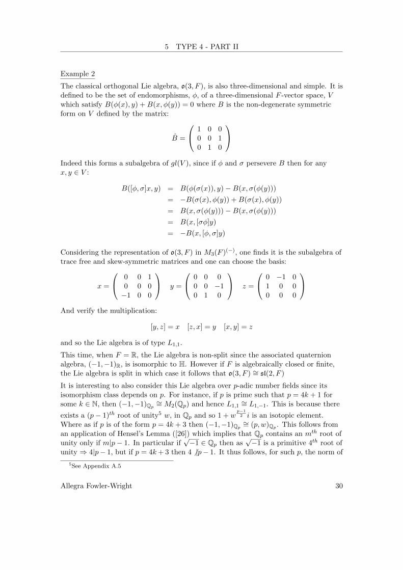
Example 2
The classical orthogonal Lie algebra, o(3, F ), is also three-dimensional and simple. It isdefined to be the set of endomorphisms, φ, of a three-dimensional F -vector space, Vwhich satisfy B(φ(x), y) +B(x, φ(y)) = 0 where B is the non-degenerate symmetricform on V defined by the matrix:
B =
1 0 00 0 10 1 0
Indeed this forms a subalgebra of gl(V ), since if φ and σ persevere B then for anyx, y ∈ V :
B([φ, σ]x, y) = B(φ(σ(x)), y)−B(x, σ(φ(y)))
= −B(σ(x), φ(y)) +B(σ(x), φ(y))
= B(x, σ(φ(y)))−B(x, σ(φ(y)))
= B(x, [σφ]y)
= −B(x, [φ, σ]y)
Considering the representation of o(3, F ) in M3(F )(−), one finds it is the subalgebra oftrace free and skew-symmetric matrices and one can choose the basis:
x =
0 0 10 0 0−1 0 0
y =
0 0 00 0 −10 1 0
z =
0 −1 01 0 00 0 0
And verify the multiplication:
[y, z] = x [z, x] = y [x, y] = z
and so the Lie algebra is of type L1,1.
This time, when F = R, the Lie algebra is non-split since the associated quaternionalgebra, (−1,−1)R, is isomorphic to H. However if F is algebraically closed or finite,the Lie algebra is split in which case it follows that o(3, F ) ∼= sl(2, F )
It is interesting to also consider this Lie algebra over p-adic number fields since itsisomorphism class depends on p. For instance, if p is prime such that p = 4k + 1 forsome k ∈ N, then (−1,−1)Qp
∼= M2(Qp) and hence L1,1∼= L1,−1. This is because there
exists a (p− 1)th root of unity5 w, in Qp and so 1 + wp−12 i is an isotopic element.
Where as if p is of the form p = 4k + 3 then (−1,−1)Qp∼= (p, w)Qp . This follows from
an application of Hensel’s Lemma ([26]) which implies that Qp contains an mth root ofunity only if m|p− 1. In particular if
√−1 ∈ Qp then as
√−1 is a primitive 4th root of
unity ⇒ 4|p− 1, but if p = 4k+ 3 then 4 6 |p− 1. It thus follows, for such p, the norm of
5See Appendix A.5
Allegra Fowler-Wright 30

6 CONSTRUCTING AN INVARIANT BILINEAR FORM ON SIMPLETHREE-DIMENSIONAL LIE ALGEBRAS
(−1,−1)Qp will be anisotropic. By uniqueness of the anisotropic norm, as mentioned insection 4.5, (−1,−1)Qp
∼= (p, w)Qp and hence L1,1∼= L−p,−w.
These examples conclude the investigation of Type 4 Lie algebras over fields ofcharacteristic not equal two. Hence classification of such is now complete. Beforelaunching into classification of three-dimensional Lie algebras over fields ofcharacteristic two, a preliminary section is included on how one may construct ainvariant bilinear form on a simple Lie algebra. It serves to extend ones insight into thestructure and characteristics of simple three-dimensional Lie algebras as well asproviding vital results for the research of simple Lie algebras over fields ofcharacteristic two.
6 Constructing an Invariant Bilinear Form on SimpleThree-dimensional Lie Algebras
The bilinear forms on L×L are in bijection with the linear maps on the tensor productL⊗L. It is helpful to use this analogue, with tensor algebras, to construct an invariantbilinear form on L. The results derived in this section are rather remarkable in thesense that they show over any field, irrespective of characteristic, there always exists asymmetric, non-degenerate, bilinear form on a simple three-dimensional Lie algebra, L.
Bilinear forms already encountered include the Killing form and the ‘structure matrix’form6. However neither are the sought after form. This is because the Killing form canbe shown to vanish in characteristic two and the ‘structure matrix’ form is constructedusing two different basis of L.
6.1 Setting the Scene
This subsection builds up the theory of exterior angles. Variations of the definitions,results and proofs of this section can be found in many algebra textbooks for exampleA. Knapp’s book, Basic Algebra, [27].
Let T (L) := ⊕∞k=0(⊗kL) be the tensor algebra of an F -algebra, L and let I(L) be theideal generated by elements of the form l ⊗ l, l ∈ L. The exterior angle is defined to bethe quotient:
∧∗ L := T (L)�I(L) with the natural projection map Π : T (L)→∧∗ L.
Definition 10 The p-fold exterior angle∧p L, is the projection:
p∧L := Π(⊗pL)
6The structure matrix is the matrix with respect to a basis e1, e2, e3 of L and the basis f1 =[e2, e3], f2 = [e3, e1], f3 = [e1, e2]. A bilinear form can then be defined by B(fi, ej) = αij wherefi =
∑3i=1 αijej .
Allegra Fowler-Wright 31

6 CONSTRUCTING AN INVARIANT BILINEAR FORM ON SIMPLETHREE-DIMENSIONAL LIE ALGEBRAS
Definition 11 For a ∈∧p L and b ∈
∧q L one defines the Grassmann product as themap ∧ :
∧∗ L×∧∗ L→ ∧∗ L, defined by:
a ∧ b := Π(a⊗ b)
Where a ∈ ⊗pL and b ∈ ⊗qL are such that Π(a) = a and Π(b) = b.
The product is well defined, for if c, d ∈ ⊗pL and e, f ∈ ⊗qL are such that Π(c) = Π(d)and Π(e) = Π(f), then c− d ∈ I(L) and e− f ∈ I(L). Thus applying Π to the identity:
c⊗ e = d⊗ f + (c− d)⊗ f + c⊗ (e− f)
Gives that Π(c⊗ e) = Π(d⊗ f), as desired. Bilinearity of the Grassmann product isequally as easy to show.
The p-fold exterior angle, together with the Grassmann product, forms an F -algebra.The following few propositions display some of the properties of the Grassmannproduct which will be of use later.
Proposition 6.1 For a ∈∧p L and b ∈
∧q L, a ∧ b = (−1)pqb ∧ a
Proof: Follows from considering the projection of (a+ b)⊕ (a+ b) �
Proposition 6.2 u1 ∧ ... ∧ up = 0 in∧p L if, and only if, u1, ..., up are linearly
dependent
Proof: See A. Knapp, [27] �
Proposition 6.3 Let L be a n dimensional F -algebra. If e1, ..., en is a basis of L, thenthe set:
{ei1 ∧ ... ∧ eip : i1 < i2 < ... < ip where ik ∈ {1, ..., n} for 1 ≤ k ≤ p}
Forms a basis of∧p L . In particular the dimension of
∧p L is(np
).
Proof: Let e1, ..., en be a basis of L. Define eI := ei1 ∧ ... ∧ eip where1 ≤ i1 < i2 < ... < ip ≤ n and I := {i1, ..., ip}. There are
(np
)distinct such elements eI .
By reordering and changing sign, any exterior product of p ei’s can be written as alinear combination of these
(np
)elements and so they span
∧p L.
Now to show linear independence; If there exists αI ∈ F such that∑αIeI = 0, where
the sum is taken over all index sets I = {i1, ..., ip} such that i1 < i2 < ... < ip. Then foreach I, define Ic := {1, 2, ..., n}\I. By proposition 6.2, eI ∧ eIc 6= 0 and ∀J 6= I, J willhave a index in common with Ic and so eJ ∧ eIc = 0. Thus by applying eIc to
Allegra Fowler-Wright 32

6 CONSTRUCTING AN INVARIANT BILINEAR FORM ON SIMPLETHREE-DIMENSIONAL LIE ALGEBRAS
∑αIeI = 0 one gets that aI = 0. It follows that aI = 0,∀I and thus the eI form a
linearly independent spanning set. �
Terminology: When a basis e1, ..., en of L is chosen, the basis ei1 ∧ ... ∧ eip wherei1 < i2 < ... < ip, shall be called the canonical basis of
∧p L.
The proposition allows one to think of∧p L as the dual space of p-multilinear,
alternating maps. To see this, consider a p-alternating multilinear map, P . One candefine the action of ei1 ∧ ... ∧ eip ∈
∧p L on P by (ei1 ∧ ... ∧ eip)(P ) := P (ei1 , ..., eip), soindeed
∧p L can be considered as a subspace of the dual space. Conversely if P is ap-alternating multi-linear map then it is uniquely determined by the values it takes onp-combinations of distinct basis elements, but as it is alternating, the order of theelements does not matter, so P is uniquely determined by the values P (ei1 , .., eip)where i1 < i2 < ... < ip. It thus follows that the dimension of the vector space ofp-multilinear alternating maps is
(np
)and as it’s dual space will has the same
dimension,∧p L must be all of it.
Another important property of the exterior angle, which will be of use later, is that alinear map between vector spaces induces a linear map between exterior angles:
Proposition 6.4 Let T : V →W be a linear map between F -vector spaces. Define∧pT on
∧p V by:∧pT (v1 ∧ ... ∧ vp) := Tv1 ∧ ... ∧ Tvp
Then ∧pT defines a linear map∧p V →
∧pW .
Proof: It needs to be shown that ∧pT is defined invariantly, i.e independent of choice ofbasis of V . But by the universal property of tensors, ⊗pT : ⊗pV → ⊗pW maps theideal I(V ) to I(W ) so ∧pT is indeed defined invariantly. Linearity is clear. �
6.2 Explicit Construction of a Bilinear Form
The 2-exterior angle allows for the extension of the study of bilinear forms on Liealgebras. In particular, since the Lie product on L, [·, ·], is an alternating bilinear mapon L, there exists a unique linear map m :
∧2 L→ L defined by:
m(a ∧ b) = [a, b]
i.e m describes the action of∧2 L on [·, ·], m(a ∧ b) = (a ∧ b)([·, ·]), as discussed in the
previous subsection.
Furthermore if L is simple, then L = [L,L] and so if [a, b] = 0 then a = γb for someγ ∈ F ∗ and thus: a ∧ b = a ∧ γa = γ(a ∧ a) = 0 also. In other words, if m(a ∧ b) = 0then a∧ b = 0 and hence m is injective. In the three-dimensional case, the dimension of∧2 L, by proposition 6.3, is
(32
)= 3 which is equal to the dimension L, so m must be
surjective and hence a bijection. In particular m−1 is well defined.
Allegra Fowler-Wright 33

6 CONSTRUCTING AN INVARIANT BILINEAR FORM ON SIMPLETHREE-DIMENSIONAL LIE ALGEBRAS
The fundamental definition of a symmetric, non-degenerate, bilinear form on a simplethree-dimensional Lie algebra can now be made:
β : L× L→3∧L
β(u, v) := m−1(u) ∧ Id(v)
Where Id : L→ L is the identity map on L and one notes that asdim(
∧3 L) =(
33
)= 1⇒
∧3 L ∼= F .
Bilinearity
Bilinearity follows from the distributivity of the Grassmann product and linearity ofm−1.
Non-degeneracy
Non-degeneracy of m is a consequence of uniqueness and the fact [·, ·] isnon-degenerate, however it can be proved directly as follows:
Proof: Assume that u ∈ L is such that β(u, v) = 0 for every v ∈ L. Since m is injective,∃!u1, u2 ∈ L such that u1 ∧ u2 = m−1(u) and so the assumption is equivalent tou1 ∧ u2 ∧ v = 0 for all v ∈ L. But this implies that u1 and u2 form a linearly dependentset with any v ∈ L by proposition 6.2, thus the dimension of L is less than or equal totwo, a contradiction. So no such u exists.
Now assume that v ∈ L is such that β(u, v) = 0 for every u ∈ L. Since m is surjective,∀u1, u2 ∈ L there exists a u ∈ L such that u1 ∧ u2 = m−1(u) and so the assumption isequivalent to u1 ∧ u2 ∧ v = 0, ∀u1, u2 ∈ L. Hence v forms a linearly dependent set withevery two elements of L, again a contradiction to dimL = 3. So no such v exists. �
Symmetry
In order to prove β is symmetric one looks at the matrix described by m. As m sendsa ∧ b to [a, b], if a basis x1, x2, x3 of L has been chosen, then the matrix representing mwith respect to the canonical basis x2 ∧ x3, x3 ∧ x1, x1 ∧ x2 of
∧2 L, is precisely thechange of basis matrix of L from [x2, x3], [x3, x1], [x1, x2] to x1, x2, x3. This matrix wasencountered in section 3.4 and is the inverse of the structure matrix. As it was shownthat the structure matrix was symmetric (without using any characteristic specificproperties), m is symmetric. Furthermore in characteristic not two, the matrix of mmay be taken to be diagonal. In characteristic equal to two one can also take thematrix of m to be diagonal, this will be proven later. The proof is omitted for now asit is not a trivial result that in a field of characteristic two, any 3× 3 symmetric matrixis diagonalisable. The proof will be the sole focus of section 7.4.
Thus, in a suitable basis, m has matrix representation of the form: a1 0 00 a2 00 0 a3
Allegra Fowler-Wright 34

6 CONSTRUCTING AN INVARIANT BILINEAR FORM ON SIMPLETHREE-DIMENSIONAL LIE ALGEBRAS
for some a1, a2, a3 ∈ F ∗.What else can be said about β? Observe that according to the matrix of m,m−1(xi) = a−1
i (xi+1 ∧ xi+2) where the indices are taken modulo 3. And so:
β : L× L m−1×Id−−−−−→ ∧2L× L ∧∗−→ ∧3L
Is such that, ∀i, j ∈ {1, 2, 3}:
β(xi, xj) = ∧∗(m−1(xi), xj)
= ∧∗(a−1i (xi+1 ∧ xi+2), xj)
= a−1i (xi+1 ∧ xi+2 ∧ xj)
Where again the indices i+ 1, i+ 2 are taken modulo 3. Hence the matrix of β has theform: a−1
1 0 0
0 a−12 0
0 0 a−13
Being able to represent β in this way is a remarkable result as it is true over any field.Following the case when the characteristic of F was not two, the Killing form is easilydetermined to have matrix representation: −2a2a3 0 0
0 −2a1a2 00 0 −2a1a2
And one sees that < u, v >= −2a1a2a3β(u, v) = −2
det(β)β(u, v),∀u, v ∈ L. In particularwhen F is characteristic two, it follows that the Killing form of L is identically zero.
The proportional relation between < ·, · > and β is as expected given the followingproposition:
Proposition 6.5 If (·, ·) : L× L→ F and (·, ·)∗ : L× L→ F are two invariant,symmetric, bilinear forms on a simple Lie algebra L, then there exists λ ∈ F ∗ such that(u, v) = λ(u, v)∗,∀u, v ∈ L
Proof: Define the operator T : L→ L by (T (u), v)∗ = (u, v), ∀u, v ∈ L. Then for α ∈ Fand u, v, w ∈ L:
(T (αu+ v), w)∗ = (αu+ v, w)
= α(u,w) + (v, w) by linearity of (·, ·)= α(T (u), w)∗ + (T (v), w)∗ by definition of T
= (αT (u) + T (v), w)∗ by linearity of (·, ·)∗
Allegra Fowler-Wright 35

7 CLASSIFICATION FOR FIELDS OF CHARACTERISTIC TWO
Thus it follows that ∀w ∈ L,
(T (αu+ v)− αT (u)− T (v), w)∗ = 0
But (·, ·)∗ is non-degenerate, hence ∀α ∈ F and ∀u, v ∈ L:
T (αu+ v)− αT (u)− T (v) = 0
i.e T is linear.
So let λ be an eigenvector of T and define Wλ = {w ∈ L : T (w) = λw}. Then Wλ is anideal of L for if u, v ∈ L and w ∈Wλ then:
(T ([w, u]), v)∗ = ([w, u], v) by definition of T
= (w, [u, v]) by invariance of (·, ·)= (T (w), [u, v])∗ by definition of T
= (λw, [u, v])∗ as w ∈Wλ
= (λ[w, u], v)∗ by invariance of (·, ·)∗
So [w, u] ∈Wλ and thus Wλ E L. As L is simple and Wλ 6= 0⇒ L = Wλ. Hence∀u, v ∈ L, (u, v) = (T (u), v)∗ = λ(u, v)∗ and as (·, ·) is non-degenerate ⇒ λ ∈ F ∗ asrequired. �
7 Classification for Fields of Characteristic Two
The classification of three-dimensional Lie algebras over a field F of characteristic twoshall now commence.
7.1 Type 1 and 2 in Characteristic Two
It is not hard to see that Type 1, Types 2(a) and Type 2(b) Lie algebras still exist andare non-isomorphic. Their properties remain valid, though one modifies the proof thatType 2(a) is restrictable by instead noting that (adx)2 = (ady)
2 = adz.
7.2 Type 3 in Characteristic Two
Since theorem 3.1 holds for fields of characteristic two, the theory of Type 3 developedin section 3.3 holds up to the identification of the three possible rational canonicalforms.
Recall that if L is a Type 3 Lie algebra then there is a basis x, y, z of L such that x, yis a basis for the abelian derived algebra, L′ and adz : L′ → L′ is an isomorphism.Furthermore if L is also of Type 3, with basis x, y, z and L′ has basis x, y then adz issimilar to adαz for some α ∈ F ∗.
Allegra Fowler-Wright 36

7 CLASSIFICATION FOR FIELDS OF CHARACTERISTIC TWO
By theorem 3.1 it can be assumed that adz has matrix A ∈ {A1, A2,c, A3,d} and adz hasmatrix B ∈ {A1, A2,e, A3,f} where c, d, e, f ∈ F ∗. Thus if adz is similar to adαz thentheir characteristic polynomials will co-incide. So the question is when does one of:
X2 − 1, X2 − c, X2 −X − d
match one of:X2 − α2, X2 − α2e, X2 − αX − α2f
Unlike the case when the characteristic is not two, the answer is not immediatelyobvious. Indeed it is still clear that as α 6= 0 it is not possible that αA3,f is similar toA1 or A2,c for any c, f ∈ F ∗, thus giving rise to one distinct family. However it is nowpossible that if α2 = e−1 that:
X2 − 1 = X2 − α2e
Though one observes that as A1 acts as the identity and αA2,e is clearly not a multipleof the identity, there can be no invertible matrix P such that P−1A1P = αA2,e, thusthe two families A1 and A2,· are still distinct.
If F is a perfect field then any member of A2,· is multiplicatively similar to A2,1.Indeed if e ∈ F ∗ then one can find α ∈ F ∗ such that e−1 = α2. Thus the invertible
matrix P =
(0 1α 0
)is such that PA2,1P
−1 = αA2,e
If F is not perfect, the family A2,· is determined by the quotient F×/F×2 as then, likein the non characteristic two case, A2,c is similar to αA2,e if, and only if, c ∈ eF×2.
It follows that for every field of characteristic two, the same classification holds as thatof the non characteristic two case and a Type 3 Lie algebra is still non-abelian,solvable, non-nilpotent, has trivial centre and is non-restrictable, as discussed before.
Examples: The following examples use knowledge of the multiplicative structure ofcertain fields, details can be found of such in Appendix A.
1. The finite field, F2n , n ∈ NAs F2n is perfect, it follows that there are the 2n + 1 non-isomorphic, Type 3, Liealgebras:
• L1
• L2,1
• L3,d for d ∈ F∗2n and there are 2n − 1 non-isomorphic members in this family.
2. The local field, F2n((t)), n ∈ NF2n((t)) is not a perfect field, moreover it actually has infinitely many squareclasses.
• L1
Allegra Fowler-Wright 37

7 CLASSIFICATION FOR FIELDS OF CHARACTERISTIC TWO
• Since there are infinitely many square classes in F2n((t)), there will beinfinitely many distinct members in the family L2,·
• L3,d for d ∈ F2n((t))∗ and as the field is infinite, the family is infinite.
7.3 Type 4 in Characteristic Two - Part I
The classification methods used previously for Lie algebras of Type 4 can not be usedsince the Killing form can be identically zero. To add to this there is also no one-to-onecorrespondence between symmetric bilinear forms and quadratic forms, and quadraticforms were the crux of the theory used previously in classification.
Observe that, using a modification of the polar form, it is possible to uniquelydetermine a symmetric bilinear form from a quadratic form:
B(x, y) = Q(x+ y)−Q(x)−Q(y)
However it is possible to have a degenerate bilinear form associated to a non-zeroquadratic forms, take Q(x) = x2 for example. Furthermore a bilinear form obtained inthis way will always be alternate since B(x, x) = Q(x)−Q(x) = 0, so not all bilinearforms can be manipulated from a polarisation of a quadratic form.
One can also obtain a quadratic form from a bilinear form via defining Q(x) = B(x, x),but Q is not uniquely determined. For instance the bilinear form B(x, y) = x+ y canhave any fully isotropic quadratic form associated to it. This clearly shows how thetheory of quadratic forms is of no real use for classification in characteristic two and iswhy the focus is now moved back onto the bilinear form.
Recall that for a Type 4 Lie algebra there is the invariant, non-degenerate, symmetricbilinear form:
β : L× L→3∧L β := m−1 ∧ Id
Where m :∧2 L→ L is the bijection sending x ∧ y 7→ [x, y] and id : L→ L is the
identity map on L. The aim is to classify this symmetric bilinear form.
Pioneers in the research of symmetric bilinear forms over fields of characteristic twoinclude A. Albert and C. Arf. Arf discovered the so called Arf invariant ofnon-degenerate quadratic forms, showing that two forms are equivalent if, and only if,their Arf invariants are equal. But, as seen, a bilinear form can serve as the polar formfor two non-equivalent (and hence different Arf invariants) quadratic forms, sounfortunately his results do not aid the study of symmetric bilinear forms. However,Albert proved a series of results ([28]) two of particular relevance being:
(1) Every non-alternating, symmetric form has a matrix equivalent to a diagonal.
(2) If F is perfect then every two non-alternate symmetric forms of equal ranks areequivalent.
Allegra Fowler-Wright 38
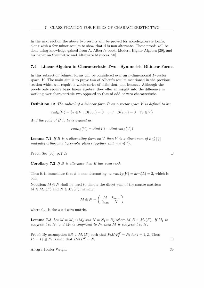
7 CLASSIFICATION FOR FIELDS OF CHARACTERISTIC TWO
In the next section the above two results will be proved for non-degenerate forms,along with a few minor results to show that β is non-alternate. These proofs will bedone using knowledge gained from A. Albert’s book, Modern Higher Algebra [29], andhis paper on Symmetric and Alternate Matrices [28].
7.4 Linear Algebra in Characteristic Two - Symmetric Bilinear Forms
In this subsection bilinear forms will be considered over an n-dimensional F -vectorspace, V . The main aim is to prove two of Albert’s results mentioned in the previoussection which will require a whole series of definitions and lemmas. Although theproofs only require basic linear algebra, they offer an insight into the difference inworking over characteristic two opposed to that of odd or zero characteristic.
Definition 12 The radical of a bilinear form B on a vector space V is defined to be:
radB(V ) = {u ∈ V : B(u, v) = 0 and B(v, u) = 0 ∀v ∈ V }
And the rank of B to be is defined as:
rankB(V ) = dim(V )− dim(radB(V ))
Lemma 7.1 If B is a alternating form on V then V is a direct sum of k ≤ [n2 ]mutually orthogonal hyperbolic planes together with radB(V ).
Proof: See [30], p27-28 �
Corollary 7.2 If B is alternate then B has even rank.
Thus it is immediate that β is non-alternating, as rankβ(V ) = dim(L) = 3, which isodd.
Notation: M ⊕N shall be used to denote the direct sum of the square matricesM ∈Mm(F ) and N ∈Mn(F ), namely:
M ⊕N =
(M 0m,n
0n,m N
)where 0s,t is the s× t zero matrix.
Lemma 7.3 Let M = M1 ⊕M2 and N = N1 ⊕N2 where M,N ∈Mn(F ). If M1 iscongruent to N1 and M2 is congruent to N2 then M is congruent to N .
Proof: By assumption ∃Pi ∈Mn(F ) such that PiMiPTi = Ni for i = 1, 2. Thus
P := P1 ⊕ P2 is such that PMP T = N. �
Allegra Fowler-Wright 39

7 CLASSIFICATION FOR FIELDS OF CHARACTERISTIC TWO
Lemma 7.4 Let M ∈Mn(F ) be symmetric. If there exists n′ ∈ N, with n′ < n, suchthat the n′ × n′ matrix, M ′ in the upper left corner of M , is invertible, then M iscongruent to a matrix of the form M ′ ⊕N .
Proof: Let M ∈Mn(F ) be symmetric. Write M =
(M ′ (M ′′)T
M ′′ M ′′′
), where M ′
∈Mn′(F ) is assumed to be invertible, M ′′′ ∈Mn−n′(F ) and M ′′ is an (n− n′)× n′matrix. Define:
P :=
(In′,n′ 0n′,n−n′
M ′′(M ′)−1 In−n′,n−n′
)Then P is invertible as det(P ) = 1.
Noting that M ′′ +M ′′ = 0, (M ′′)T + (M ′′)T = 0 and (M ′)−T = (M ′)−1 (since M ′ issymmetric), one calculates that:
PMP T =
(M ′ 00 N
)Where N := M ′′(M ′)−1(M ′′)T +M ′′′. �
Lemma 7.5 A bilinear form is non-alternating if, and only if, its matrix cannot berepresented by a zero diagonal matrix.
Proof: (⇒) The contrapositive shall be proved. Let B be a bilinear form such that, insome basis {e1, ..., en} of V , it has a zero-diagonal matrix M = (mij)i,j . Then for anyx ∈ V there exists ai ∈ F such that x =
∑i aiei, and so:
B(x, x) =∑i,j
aiajB(ei, ej) =∑i 6=j
aiajmij = 2∑i<j
aiajmij = 0
Hence B is alternate.
(⇐) The contrapositive again shall be proved. If B is an alternating bilinear formthen, in any basis {e1, ..., en}, its matrix M = (mij)i,j is such that mii = B(ei, ei) = 0for 1 ≤ i ≤ n. Thus M is zero diagonal. �
Notation: From now on, the matrix
(0 11 0
)will be denoted by J .
Lemma 7.6 For any a ∈ F ∗, the matrices A =
(0 aa 0
)and J are congruent.
Proof: Let P =
(1 00 a−1
), then P is invertible and PAP T = J. �
Notation: Let Enij denote the n× n identity matrix with its ith and jth rowinterchanged.
Allegra Fowler-Wright 40

7 CLASSIFICATION FOR FIELDS OF CHARACTERISTIC TWO
Observe that Enij is invertible with (Enij)−1 = (Enij)
−T = Enij . Furthermore multiplying
a matrix, M , on the right by Enij has the effect of interchanging M ’s ith and jth row,
whilst multiplying M on the left by Enij , interchanges M ’s ith and jth column.
Proposition 7.7 Let k ∈ N. If M ∈M2k(F ) is a zero diagonal, non-singular andsymmetric matrix, then M is congruent to ⊕k1J .
Proof: By induction. Let ∆(k) be the statement ‘for all n ∈ N such that n ≤ k, ifM ∈M2n(F ) is zero diagonal, non-singular and symmetric, then it is congruent to⊕n1J ’.
Clearly ∆(1) is true by lemma 7.6. Assume ∆(k − 1) is true and choose anyM = (mij)i,j ∈M2k(F ) which is zero diagonal, non-singular and symmetric. Let i, j besuch that mij 6= 0, then M ′ = E2k
2jE2k1iME2k
1i E2k2j is congruent to M and has mijJ in its
upper left hand corner. By lemma 7.4, M ′, and hence M , is congruent to a matrix ofthe form (mijJ)⊕ P for some P ∈M2k−2(F ) which will also be a zero diagonal,non-singular and symmetric matrix. By the inductive hypothesis P is congruent to adirect sum of k − 2 blocks J . Thus M is congruent to (mijJ)⊕ P which by lemma 7.3is congruent to (mijJ)⊕k−2
1 J and, by an application of lemma 7.3 again, this iscongruent to ⊕k1J . Therefore ∆(k) holds and the induction is complete. �
Proposition 7.8 Let a ∈ F ∗ and k ∈ N. Then the matrix (aI1)⊕k−11 J is congruent to
the diagonal matrix aI2k−1
Proof: By induction. Let ∆(k) be the statement ‘for all a ∈ F ∗ and for every n ∈ Nsuch that n ≤ k, (aI1)⊕n−1
1 J is congruent to the diagonal matrix aI2n−1’.
Trivially ∆(1) is true and ∆(2) is true since QAQT = aI3 where Q is the invertiblematrix: 1 1 0
1 0 a1 1 a
Assume ∆(k − 1) is true for k ≥ 3. Then for any a ∈ F ∗, A := (aI1)⊕k−1
1 J can bewritten in the form A = Ak−2 ⊕ J where Ak−2 := aI1 ⊕k−2
1 J . By the inductionhypothesis Ak−2 is congruent to the diagonal matrix aI2k−3 and by lemma 7.3 itfollows that A is congruent to aI2k−3 ⊕ J . Now, consider the bottom 3× 3 matrix ofaI2k−3 ⊕ J , which has the form:
aI1 ⊕ J =
a 0 00 0 10 1 0
By the k = 2 case, this 3× 3 matrix is congruent to aI3 and by lemma 7.3 it followsthat aI2k−4 ⊕ (aI1 ⊕ J) is congruent to aI2k−1. Hence, in turn, A is congruent toaI2k−1. Thus ∆(k) is true and the induction is complete. �
Enough theory has now been developed to prove one of Albert’s theorem:
Allegra Fowler-Wright 41

7 CLASSIFICATION FOR FIELDS OF CHARACTERISTIC TWO
Theorem 7.9 For any non-degenerate, non-alternate, symmetric bilinear form, thereis a basis such that it’s matrix representation is diagonal.
Proof: By induction, it shall be proved that any symmetric n× n non-singular matrix,M , with at least one non-zero diagonal entry is congruent to a diagonal matrix. Theinduction is done on n where M ∈Mn(F ).
If n = 1 then M = (m11) and trivially M is diagonal.
Assume it is true for all k < n, let M = (mij)i,j ∈Mn(F ) and let k be such thatmkk 6= 0. Then M ′ = En1kMEn1k is an n× n symmetric, non-degenerate matrix withmkk in the top left corner. By lemma 7.4, since (mkk) is invertible, M ′ is congruent toa matrix of the form (mkkI1)⊕N with N ∈Mn−1(F ). Clearly N will also besymmetric and non-singular. There are two cases to consider:
Case 1: If N has one non-zero diagonal entry, then, by the induction assumption N iscongruent to a diagonal matrix and hence so is M by lemma 7.3.
Case 2: If N is zero-diagonal, then by lemma 7.5, N represents an alternating bilinearform and so, by corrollary 7.2, rank(N) is even. Thus in this case we must have that nis odd else N would be non-singular which implies that M is too, contradiction. It
follows from proposition 7.7 that N ∈Mn−1(F ) is congruent to the direct sum ⊕n−12
1 Jand hence by proposition 7.3 M is congruent to the matrix:
(mkkI1)⊕n−12
1 J
But by proposition 7.8, this is congruent to mkkIn, a diagonal matrix, which concludescase 2.
So in both cases, M ∈Mn(F ) is congruent to a diagonal matrix and thus the inductionis complete.
The main result of the theorem now directly follows as any non-degenerate,non-alternate, symmetric bilinear form has a symmetric, non-singular matrix which, bylemma 7.5, has at least one non-zero diagonal entry. �
Remark: Referring back to section 6.2, it was assumed, without proof, that m could bediagonalised in characteristic two. The above theorem is a proof of this and thus thestructural properties of β that followed will always hold. In particular it means thatthe Killing form of a Type 4 Lie algebra in characteristic two will always be identicallyzero.
Using the previous theorem, part of Albert’s other result can be derived:
Corollary 7.10 If F is a perfect field then every non-degenerate, non-alternate,symmetric bilinear form has a basis such that it’s matrix is the identity.
Proof: First note that if F is perfect then a matrix M ∈Mn(F ), is equivalent to aMfor all a ∈ F ∗. Indeed, aM = (aIn)M(aIn), where a ∈ F ∗ is such that a2 = a.
Allegra Fowler-Wright 42

7 CLASSIFICATION FOR FIELDS OF CHARACTERISTIC TWO
From theorem 7.9, if γ is a non-degenerate, non-alternate, symmetric bilinear form,then a basis can be chosen so that its representing matrix is diagonal. So there existsai ∈ F ∗ such that γ’s matrix representation is D(a1, a2, ..., an).
For each i, pick bi ∈ F ∗ such that (bi)2 = ai. Then P = D(b−1
1 , b−12 , ...b−1
n ) is such thatPMP T = In. �
Remark: The above corollary can easily be adapted to show that the conjugacy class ofa diagonal matrix over a general field of characteristic two depends only on the classesof its diagonal entries in F×/F×2. Indeed if M = D(a1, a2, ..., an) then M is congruentto D(a′1, a
′2, ..., a
′n) whenever a′i ∈ aiF×2 for i = 1, .., n. By considering the change of
basis matrices Eij , one see’s further that D(a1, a2, ..., an) is also congruent toD(a′σ(1), a
′σ(2)..., a
′σ(n)) for any σ ∈ Sn.
Theorem 7.11 A matrix in Mn(F ) is congruent to the identity matrix only if it’sdiagonal entries are the squares of elements in F ∗.
Proof: If M ∈Mn(F ) is such that PInPT = M for some invertible
P = (pij)i,j ∈Mn(F ), then the kth diagonal entry of M , is∑n
i=1(pik)2 = (
∑ni=1 pik)
2.�
7.5 Examples over Specific Fields
Finding when two diagonal matrices are congruent is a problem which requires thestructural properties of a field, and so is not solvable over a general field. Thuscongruence classes over specific fields shall now be considered.
1. The finite field F2n , n ∈ NF2n is a perfect field and so by corollary 7.10, there is only one equivalence classof bilinear forms, those of whom whose matrix representation can be described bythe identity.
Allegra Fowler-Wright 43
7 CLASSIFICATION FOR FIELDS OF CHARACTERISTIC TWO
2. Simple transcendental extensions of F2n
Let F = F2n(t), where t is transcendental over F2n . In this case(F2n(t))×2 = F2n(t2)×. In order to see this, take any b ∈ F2n(t) then b is of theform b1 + b2t+ ....+ bnt
n for some bi ∈ F2n and n ∈ N and so:
b2 = (b1 + b2t+ ....+ bntn)2
= b21 + b22t2 + ...+ b2nt
2n ∈ F2n(t2)
Therefore it follows that:
If a ∈ (F2n(t))2 then ∃b ∈ F2n(t) such that b2 = a
⇔ a ∈ F2n(t2)
Since every element in the multiplicative quotient group F2n(t)×/F2n(t2)× can bewritten in the form (a+ bt)Fq(t2)× for some a, b ∈ F2n , it follows thatF2n(t)×/F2n(t2)× = {1, t} and thus |F2n(t)× : F2n(t2)×| = 2. Consequently thereare 4 conjugacy classes of diagonal matrices, namely: 1 0 0
0 1 00 0 1
t 0 00 1 00 0 1
t 0 00 t 00 0 1
t 0 00 t 00 0 t
3. The local field F2n((t))
From Appendix A.4, |F2n((t))× : F2n((t))×2| is infinite and so there are infinitelymany non-conjugate diagonal matrices.
Interestingly, one finds that square elements in F2n((t)) are precisely the elementsin F2n((t2)). This is shown by considering b ∈ F2n((t)). b has the form∑∞
i=−m biti for some bi ∈ F2n and m ∈ N0. Defining pn(b) :=
∑ni=−m bit
i, for eachn ∈ N, the sequence (pn(b))n is such that:
limn→∞
pn(b) = b
Convergence being with respect to the absolute value induced by the degreevaluation on F2n((t)). Also:
pn(b)2 = (
n∑i=−m
biti)2 =
n∑i=−m
bit2i ∈ F2n((t2))
Therefore it follows that:
If a ∈ (F2n((t)))2 then ∃b ∈ Fq((t)) such that b2 = a
⇔(
limn→∞
pn(b))2
= a
⇔ limn→∞
(pn(b))2 = a
⇔ a ∈ F2n((t2))
Allegra Fowler-Wright 44

7 CLASSIFICATION FOR FIELDS OF CHARACTERISTIC TWO
7.6 Type 4 in Characteristic Two - Part II
It has been proved that if L is a Type 4 Lie algebra then β(x, y) = m−1(x) ∧ y is abilinear form on L and a basis of L may be chosen such that β is represented by adiagonal matrix over M3(
∧3 L).
Notation: A diagonal matrix representing β shall be denoted by Mβ.
Theorem 7.12 Two three-dimensional, simple Lie algebras are isomorphic if, andonly if, there exists an invertible matrix A such that det(A)A−TMβA
−1 is congruent toMγ, where β and γ are the respective bilinear forms, as constructed in section 6.2, ofthe Lie algebras.
Remark: Recall the relation Mφ(x),φ(y),φ(z) = det(A)A−TMx,y,zA−1 was shown to hold
between the structure matrices of two isomorphic Lie algebras when the characteristicof F was not two. Hence, when one remembers that β’s matrix representation is theinverse to that of the structure matrix ,when in diagonal form, the above resultbecomes somewhat less surprising.
Proof: Let L and R be two isomorphic three-dimensional, simple Lie algebras withrespective bilinear forms β : L× L→ ∧3L and γ : R×R→ ∧3R. Fix a basis e1, e2, e3
of L such that Mβ is diagonal and choose a basis f1, f2, f3 of R such thate1 ∧ e2 ∧ e3 = f1 ∧ f2 ∧ f3.
Let φ : L→ R be an isomorphism between L and R and let A = (αij)i,j be its matrixrepresentation. From proposition 6.4 ,the induced map: ∧3φ : ∧3L→ ∧3R is linear,which gives the following commutative diagram:
L× L β−−−−→ ∧3Lyφ×φ y∧3φR×R γ−−−−→ ∧3R
Thus γ = ∧3φ ◦ β ◦ (φ−1 × φ−1).
From linear algebra, A−TMβA−1 describes the bilinear form7,
β ◦ (φ−1 × φ−1) : R×R→ ∧3L, in the basis φ(e1), φ(e2), φ(e3) of R.
As the dimension of ∧3L and ∧3R are both one, the induced linear map ∧3φ of φ mustact by multiplication in F ∗. So let λ ∈ F ∗ be such that ∧3φ = λ. Then, since
7Indeed, if v denotes a vector in F 3×1 representing an element v = v1e1 + v2e2 + v3e3 in L, thenAv = v′, where v′ is a column vector denoting the element φ(v) in the basis φ(e1), φ(e2), φ(e3) of R. Thus
vTMβv = v′TA−TMβA
−1v′. So A−TMβA−1 describe the bilinear form β in the basis φ(e1), φ(e2), φ(e3)
of R.
Allegra Fowler-Wright 45

7 CLASSIFICATION FOR FIELDS OF CHARACTERISTIC TWO
φ(ei) =∑3
j=1 αjifj it follows that:
∧3φ(e1 ∧ e2 ∧ e3) := φ(e1) ∧ φ(e2) ∧ φ(e3)
=∑
jk=1,2,3
αj1,1fj1 ∧ αj22fj2 ∧ αj33fj3
=∑σ∈S3
ασ(1)1fσ(1) ∧ ασ(2)2fσ(2) ∧ ασ(3)3fσ(3)
=∑σ∈S3
sgn(σ)ασ(1)1ασ(2)2ασ(3)3(f1 ∧ f2 ∧ f3)
=: det(A)(f1 ∧ f2 ∧ f3) = det(A)(e1 ∧ e2 ∧ e3)
Where the third equality follows from the fact that if ik = ij for some k 6= j thenfj1 ∧ fj2 ∧ fj3 = 0 (proposition 6.2) and so the sum can be taken over indices i1, i2, i3such that (i1, i2, i3) is a permutation of (1, 2, 3). The fourth equality then followsbecause any permutation is a product of transpositions and any transposition changesthe sign of the exterior product (proposition 6.1).
Thus λ = det(A) and det(A)A−TMβA−1 represents the bilinear form
γ = ∧3φ ◦ β ◦ (φ−1 × φ−1) with respects to the basis φ(e1), φ(e2), φ(e3) of R. But thisimplies that Mγ must be congruent to the matrix det(A)A−TMβA
−1. �
From the theorem it follows that the isomorphism classes of Type 4 Lie algebras aredetermined by the classes of multiplicatively congruent diagonal matrices over F . Asalready seen, these classes depend on the structural properties of the base field. So allthat can be said about a general field F , of characteristic two, is that there is at leastone simple three-dimensional Lie algebra, it’s bilinear form arising from the congruencyclass of the identity matrix. By considering such a Lie algebras structure matrix, onecan see it has a basis x, y, z such that multiplication is defined by:
[x, y] = z [x, z] = y [y, z] = x
Examples
1. The finite field F2n , n ∈ NThere is only one Type 4 Lie algebra, with multiplication as defined above.
2. Simple transcendental extensions of F2n
Let F = F2n(t) where t is transcendental over F2n
From section 7.5 there are four conjugacy classes of diagonal matrices thus atmost four distinct Type 4 Lie algebras. In order to determine whether two of theconjugacy classes can be multiplicatively congruent, one can look at the possibledeterminants a multiplicative congruence relation would give. It turns out that ineach case, a multiplicative congruence would lead to the contradiction that t
Allegra Fowler-Wright 46

7 CLASSIFICATION FOR FIELDS OF CHARACTERISTIC TWO
satisfies a polynomial equation over F2n of finite degree. Thus the four conjugacyclasses give rise to four non-isomorphic Lie algebras.
So, if L is a Type 4 Lie algebra then there exists a basis x, y, z of L, such that Lhas multiplication defined by one of:
[x, y] = z [z, x] = y [y, z] = x
[x, y] = z [z, x] = y [y, z] = t−1x
[x, y] = z [z, x] = t−1y [y, z] = t−1x
[x, y] = t−1z [z, x] = t−1y [y, z] = t−1x
3. The local field F2n((t))
There are infinitely many Type 4 Lie algebras since there are infinitely manycongruency classes of diagonal matrices.
7.7 Quaternion Algebras in Characteristic Two
Despite the fact that the correspondence between quadratic forms and symmetricbilinear forms breaks down in characteristic two, one may still question whether thereis a link between quaternion algebras and Type 4 Lie algebras. This subsection willaim to answer this question.
One should note that it is not natural to try and define a generalised quaternionalgebra over a field of characteristic two, as in section 4. This is because, by definition,any such algebra will be a commutative algebra since ij = −ji = ji, losing thequaternion algebra’s distinctive structure and properties. In particular the involutionof conjugation, q → q becomes the identity map. And so, a new definition is requiredto construct the analogue of a quaternion algebra in characteristic two, coupled with anew involution.
The following definition is for a field of any characteristic.
Definition 13 Given a, b ∈ F such that 1 + 4a 6= 0 and b 6= 0, define the Huppertalgebra, denoted H(a, b), over F to be the four-dimensional vector space with basis{1, i, j, ij} and multiplication defined by:
i2 = i+ a j2 = b ji = 1− ij
This definition is a variant of the definition in Classical Groups and GeometricAlgebra, [30]. It can easily be verified that H(a, b) is an associative algebra and thatthe definition coincides with that of a quaternion algebra over a field of characteristicnot two. To see the latter, set I := i− 1
2 and J := j. Then the algebra spanned by
{1, I, J, IJ} has defining multiplication: I2 = a+ 14 , J
2 = b and IJ = ij − j2 = −JI, in
other words the span of the linearly independent set {1, I, J, IJ} is Q(a+ 14 , b).
Allegra Fowler-Wright 47

7 CLASSIFICATION FOR FIELDS OF CHARACTERISTIC TWO
Definition 14 For x = α+ βi+ γj + δij ∈ H(a, b) define H-conjugation, x 7→ x by:
x = x+ β ∈ H(a, b)
It can be shown that H-conjugation is an involution and thus one can define trace andnorm forms on H(a, b) by:
N : H(a, b)→ F N(x) := xx
Tr : H(a, b)→ F Tr(x) := x+ x
Finally, the space of pure ‘Huppertions’ is defined as:
H0(a, b) := {x ∈ H(a, b) : Tr(x) = 0}
Clearly x = α+ βi+ γj + δij ∈ H0(a, b)⇔ β = 0, so H0(a, b) is three-dimensionalF -vector space with basis {1, j, ij}.As with the space of pure quaternions, one can define a three-dimensional Lie algebrafrom the space of pure Huppertions: H0(a, b)(−) = F.1 + Fj + Fij. However it is notsimple. Indeed the centre of H0(a, b) is non-trivial, precisely it is F . Also the derivedalgebra of H0(a, b)(−) is Fj since [j, ij] = j. Thus H0(a, b)(−) is a three-dimensional Liealgebra with a non-zero centre and one-dimensional derived algebra, of which is notcontained in it’s centre. This is precisely the definition of a Type 2(b) Lie algebra.Since there is only one Type 2(b) Lie algebra, up to isomorphism, it follows thatH0(a, b)(−) ∼= H0(c, d)(−) for every a, c, b, d ∈ F ∗.Another three-dimensional Lie algebra can also be constructed by considering thequotient: H(a, b)/F . This is an associative algebra with zero centre and the basisiF, jF, ijF has defining multiplication:
[iF, jF ] = 0 [iF, ijF ] = iF [jF, ijF ] = jF
From the multiplication identities, one can clearly see that the derived algebra of(H(a, b)/F )(−) is two-dimensional and its centre is zero. Thus, under this papersclassification, it is a Type 3 Lie algebra of isomorphismtype L1.
Although a Huppert algebra can be used to create a Type 2 and a Type 3 Lie algebra,it is not possible to manipulate a Type 4 Lie algebra out of it. The fact thatquaternion algebras can not be linked to Type 4 Lie algebras in any way over a field ofcharacteristic two, a surprising result considering that the isomorphism classes of Type4 Lie algebras over fields of odd or zero characteristic were completely determined bythem.
7.8 Representations of Type 4 Lie algebras
Recall that the Type 4 Lie algebras are the simple three-dimensional Lie algebras.Examples of Type 2 and Type 3 Lie algebras, over a field of characteristic two, have
Allegra Fowler-Wright 48

7 CLASSIFICATION FOR FIELDS OF CHARACTERISTIC TWO
already been given in section 7.7, therefore the objective is now to give arepresentation of a Type 4 Lie algebra.
Using Chevalley basis’s and reduction modulo p the well known classical andexceptional ([10], Chapter 13) simple Lie algebras over fields of characteristic zero canbe used to form Lie algebras over fields of characteristic p. However these are notalways simple. In fact, it can be shown that in characteristic two, A2
∼= sl(3, 2) is theonly classical Lie algebra of dimension less than, or equal to, nine that remains simple.
It was E. Witt, in the 1930s, who was the first to discover a finite-dimensional,non-classical, simple Lie algebra over a field of prime characteristic, today known asthe Witt Lie algebra, W (1; 1). At the time, Witt never published his example, orgeneralisations of it and it was H. Zassenhaus and Chang Ho Yu who were the first topublish information on Witt’s work, [32]. Today, Witt Lie algebras are referred to assimple Lie algebras of ‘Cartan type’. The construction of such a Lie algebra is givenbelow with Lie algebras of small dimension, [15], providing the foundationalknowledge. The only assumption imposed on F is that it has characteristic p > 0.
Let O(m) denote the commutative, associative algebra over F , generated by theelements xki , 1 ≤ i ≤ m, k ∈ N0 which satisfy the relations:
x0i = 1 and xki x
li =
(k + l
k
)xk+li for 1 ≤ i ≤ m and ∀k, l ∈ N0
The elements x(k) := xk11 ...xkmm where (k) denotes the multi-index (k1, .., km) ∈ Nm0 ,
form a basis for O(m).
For n = (n1, ..., nm) ∈ Nm0 , a finite-dimensional subalgebra of O(m) can be defined as:
O(m;n) := spanF {x(k) : 0 ≤ ai < pki}
One can also define derivations on O(m), denoted by Di, by: Dix(k) = x(k−εi) where εi
is the m-tuple with 1 in it’s ith position and 0 elsewhere. This leads to the penultimatedefinition of the infinite-dimensional Witt Lie algebra of Cartan type:
W (m) := spanF {x(k)Di : (k) ∈ Nm0 }
Together with the Lie product:
[x(k)Di, x(l)Dj ] = x(k)Dix
(l)Dj − x(l)Djx(l)Di
Definition 15 For m ∈ N and n ∈ Nm0 , n 6= 0, the finite-dimensional Witt Lie algebraof Cartan Type, W (m;n) is defined as:
W (m;n) := spanF {x(k)Di : 1 ≤ kj < pnj , 1 ≤ i ≤ m}
One sees that not only is O(m;n) a subalgebra of O(m) and W (m;n) a subalgebra ofW (m), but also that W (m;n) = W (m) ∩Der(O(m;n)).
Allegra Fowler-Wright 49

7 CLASSIFICATION FOR FIELDS OF CHARACTERISTIC TWO
Theorem 7.13 (1) W (m;n) is simple except when m = 1 and p = 2.
(2) The set of elements: {x(k)Di : 0 ≤ kj < pnj , 1 ≤ i, j ≤ m} determines a basis ofW (m;n) and hence dimFW (m;n) = mpn1+...+nm.
The proof of this theorem requires the notion of a graded Lie algebra. An introductionto this notion and a complete proof can be found in Chapter 4 of Strade andFarnsteiner, [31].
Remark: W (1; 1) is often referred to as the p-dimensional Witt algebra.
Observe that in characteristic p > 3, no Witt Lie algebra is three-dimensional. If p = 3the Witt algebra, W (1; 1), is three-dimensional and, by theorem 7.13, it is simple. Ifp = 2 the Witt algebra W (1; 2) is four-dimensional and not simple, however its derivedalgebra is three-dimensional and simple, as shall now be seen:
W (1; 2) over a field of characteristic two
W (1; 2) := spanF {xkD : 0 ≤ k < 22}= spanF {D,xD, x2D,x3D}
This has defining Lie products:
[D,xD] = D [D,x2D] = xD [xD, x2D] = x2D
[D,x3D] = 0 [xD, x3D] = 0 [x2D,x3D] = 0
This confirms theorem 7.13 for n = 2, since a non-zero, proper ideal can be generatedby x3D. However the derived algebra:(
W (1; 2))′
= spanF {D,xD, x2D}
Is a three-dimensional Lie algebra with defining multiplication:
[a, b] = a [a, c] = b [b, c] = c
Where a := D, b := xD, c := x2D. Because(W (1; 2)
)′is equal to it’s derived algebra, it
is not solvable and thus it is simple8. As expected, it is true that the bilinear form, β(as constructed in section 6.2), on
(W (1; 2)
)′can be taken to be the identity. To
explicitly see this, take the basis a+ b+ c, a+ b, b+ c of(W (1; 2)
)′. In this basis,
multiplication is defined by:
[a+ b+ c, a+ b] = b+ c [a+ b+ c, b+ c] = a+ b [a+ b, b+ c] = a+ b+ c
Using the relationship between a Lie algebras diagonal structure matrix and its bilinearform, it follows that, in this basis, β has identity representation.
8It has been shown that not solvable implies simple in the three-dimensional case.
Allegra Fowler-Wright 50

8 Results
51

The following table compares the classification in this paper to that of the Bianchi classification over R. The two infinitefamilies are in bold:
Bianchi Classification Type Sub-family
I 1
II 2 (a)
III 2 (b)
IV 3 L3,− 14
V 3 L1
V I 3 L3,d where d ∈ R is such that d > −14
VI0 3 L2,1
V II 3 L3,d where d ∈ R is such that d < −14
VII0 3 L2,−1
VIII 4 L1,−1
IX 4 L1,−1
Note how the sub-family L3,d is classified into three separate families in the Bianchi classification. This is done byconsidering the action of adz on L′3,d where z /∈ L′3,d. Assuming that z ∈ L3,d is chosen such that it’s matrix M , of adz, is in
canonical form, then if d = −14 , M has two equal, non-zero, eigenvalues. Whereas if d > −1
4 then M has two real, non-zeroeigenvalues which have non-zero sum. Finally if d < −1
4 , then M has two non-real and non-imaginary eigenvalues.
52

A FIELDS AND THEIR MULTIPLICATIVE GROUPS
A Fields and their Multiplicative Groups
A.1 Algebraically Closed Fields
The main thing to remark about an algebraically closed field, K, is that it is perfectand so K× = K×2 and |K× : K×2| = 1.
A.2 The Real Numbers
The real number field is an example of a field which has characteristic zero but is notalgebraically closed.
R has precisely two square classes with representations 1 and -1. Indeed, every elementin the multiplicative group R× can be written as a product sgn(r)|r| wheresgn(r) ∈ {−1, 1} and |r| ∈ R×>0 a. Furthermore the logarithmic function describes anisomorphism between R×>0 and the additive group, R+. Thus it follows that:
R× ∼= {±1} × R+
It is easy to verify that R×2 ∼= R+ R×2 = R+ and so R×/R×2 = {±1}.
A.3 Finite Fields
For any prime p and any n ∈ N, there exists a unique (up to isomorphism) field oforder pn. Let q := pn.
First consider the case when p > 2. The map x 7→ x2 is a homomorphism ofmultiplicative groups F×q → F×2
q with kernel {±1}. Hence it follows from the firstisomorphism theorem that |F×q | = 2|F×2
q | i.e |F×q : F×2q | = 2.
When p = 2, the Frobenius map is an isomorphism, hence F×q = F×2q and so
|F×q : F×2q | = 1.
A.4 The Local Field Fq((t))
Fq((t)) is the completion of the global field Fq(t), with respect to the degree valuation.In other words, the degree valuation defined by: w(f) := min{i : ai 6= 0} forf(t) =
∑ki=0 ait
i ∈ Fq[t] is extended, in the obvious way, to become a normalisedvaluation on Fq(t). Fq((t)) is then the w-completion of Fq(t) with respect to w, itconsists of elements of the form
∑∞i=−k ait
i where ai ∈ Fq and k ∈ N0.
Proposition A.1 Let q = pn where p > 2 is prime, then:
(i) Fq((t))× = F×q × < t > ×U where U := {a ∈ Fq((t))× : a = 1 + o(t)}(ii) U = U2
Allegra Fowler-Wright 53
A FIELDS AND THEIR MULTIPLICATIVE GROUPS
Proof (i) It is clear that for a ∈ Fq((t))×, a can be written in the form a = uvtw(a),where u ∈ Fq and v ∈ U , it thus ollows that Fq((t))× = Fq× < t > ×U .
(ii) Proof by induction, an easy exercise. �
Thus, since |F×q : F×2q | = 2, it follows that |Fq((t))× : Fq((t))×2| = 4. The four square
classes shall be given the canonical representations 1, u, t, ut where F×q /F×2q = {1, u}.
The case where q = pn and p = 2 is slightly more technical as part (ii) is not true andU2 is harder to compute. However in F. Lorenz book ([23], p85), a proof is given, bycontradiction that the index |Fq((t))× : Fq((t))×2| is in fact infinite.
A.5 The p-adic Number Fields
The p-adic number field, Qp, is the completion of the field Q with respect to theabsolute value, | · |p : Q→ pZ, |x|p := p−vp(x) where vp is the p-adic valuation on Qdefined by vp(x) := n for x = pn ab , a, b, p coprime. One can write:
Qp := {∞∑i=n
aipi : ai ∈ {0, 1, .., p− 1} n ∈ Z}
The ring of integers of Qp can similarly be defined as:
Zp := {∞∑i=0
aipi : ai ∈ {0, 1, .., p− 1}}
= {x ∈ Qp : |x|p ≤ 1}
It is worth remarking that Zp is a discrete valuation ring with maximal ideal pZp andresidue field Zp/pZp ∼= FpThe following results have been extracted from The Classical Fields, [33].
Proposition A.2 Let p > 2, be prime. Then:
(i) U = 1 + pZp is a multiplicative subgroup of Q×p(ii) Qp contains a (p− 1)th root of unity, w
(iii) Q×p =< p > × < w > ×U
Only (i) and (iii) shall be proved.
Proof: (i) The natural ring homomorphism Zp → Zp/pZp, restricted to Zp\pZp ismultiplicative with kernel U . Since Zp\pZp = Z×p it follows that U is also amultiplicative subgroup of Q×p(iii) The surjective group homomorphism | · |p : Q×p → pZ has kernal Z×p , henceQ×p =< p > ×Z×p . From (ii) it follows that Z×p can be written as a disjoint union ofcosets wi + pZp, i = 0, .., p− 2. Now, as:
wiU = wi + wipZp = wi + pZp ⇒ Z×p =< w > ×U
Allegra Fowler-Wright 54
A FIELDS AND THEIR MULTIPLICATIVE GROUPS
And so the result immediately follows. �
Theorem A.3 Let p > 2, prime. Then Q×2p =< p2 > × < w2 > ×U1 and Q×p /Q×2
p
consists of four square clssses with representations 1, w, p, wp.
Proof: From the proposition A.2 one has the product decomposition:
Q×2p =< p2 > × < w2 > ×U2
The result now follows from the observation that U2 = U since U = 1 + Zp ∼= Z+p and
2Z+p = Z+
p (2 is a unit in the ring Zp, |2|p = 1). Combining coset representatives offactors of Q×2
p in the corresponding factors of Q×p gives the system of representations.�
So for p 6= 2, the theorem shows that |Q×p : Q×2p | = 4. A similar, but more involved
method can be used for the case p = 2, however, for variation, a different approachedshall be used for when p = 2:
Lemma A.4 If x =∑∞
i=0 ai2i ∈ Z×2 , then a0 = 1
Proof: x ∈ Z×2 ⇔ x ∈(Z2/2Z2)× ∼= F×2 ⇔ a0 = 1
Theorem A.5 Z×2 /Z×22∼=(Z/8Z
)×Proof: ([24]) Consider the map φ : Z2 → Z/8Z defined byφ(∑∞
i=0 ai2i) := a0 + 2a1 + 4a2. Clearly φ is surjective and for x =
∑∞i=0 ai2
i andy =
∑∞i=0 bi2
i in Z2:
φ(xy) = φ(a0b0 + (a0b1 + b0a1)2 + (a0a2 + b0b2 + a1b1)4 + ...)
= a0b0 + (a0b1 + b0a1)2 + (a0a2 + b0b2 + a1b1)4
= (a0 + a12 + a24)(b0 + b12 + b24)
= φ(∞∑i=0
ai2i)φ(
∞∑i=0
bi2i) = φ(x)φ(y)
So φ is a ring epimorphism. In particular the restrictions of φ to Z×2 →(Z/8Z
)×and
Z×22 →
(Z/8Z
)×2are well defined epimorphisms. Since
(Z/8Z
)×2= {1}, it follows that
one can define a group epimomorphism ψ : Z×2 /Z×22 →
(Z/8Z
)×.
ψ is also injective. To see this, consider an element z ∈ Ker(ψ). Writing z =∑∞
i=0 zi2i,
then the condition z ∈ Ker(ψ) implies z0 = 1 and z1 = z2 = 0, thus
Allegra Fowler-Wright 55

B RESTRICTED LIE ALGEBRAS
z = 1 + 23∑∞
i=0 z3+i2i = 1 + 8y, where y ∈ Z2. The aim is to show that z, or
equivalently 1 + 8y, is a square in Z2. Thus consider:
(1 + 8y)12 =
∞∑i=0
(1/2
i
)(8y)i
=
∞∑i=0
ai(2y)i where ai :=
(1/2
i
)4i
It is left as an exercise to the reader to show that ∀i ∈ N0, v(ai)2 ≥ 0 and henceai ∈ Z2. Convergence of the sum then follows from considering the partial sumsSn :=
∑ni=0 ai(2y)i since, for n > m one has:
|Sn − Sm|2 = |n∑
i=m+1
aiyi2i−m|2|2m|2
≤ 1.2−m
So (Sn)n is a cauchy sequence with respect to the 2-adic norm and hence, as Z2 is
complete, ∃z12 ∈ Z2 such that z
12 = (1 + 8y)
12 ⇒ z ∈ Z×2
2 , thus proving thatKer(ψ) = Z×2
2 .
It has been shown that ψ is an injective epimorphism and hence an isomorphism andso Z×2 /Z
×22∼=(Z/8Z
)×, as required. �
Theorem A.6 Q×2 /Q×22∼= Z/2Z× Z×2 /Z
×22
Proof: Recall that Z2 is a discrete valuation ring and hence every element in the ringQ×2 can be written uniquely as a product of an element of Z2 and a power of 2. Hencethe map γ : Q×2 → Z+ ×Z×2 defined by γ(2ia) = (i, a), is well defined. Clearly γ is bothinjective and surjective. Thus there is the induced isomorphismQ×2 /Q
×22 → Z/2Z× Z×2 /Z
×22 �
By theorem A.5 and A.6, Q×2 /Q×22∼= Z/2Z× Z×2 /Z
×22∼= Z/2Z×
(Z/8Z
)×. As(
Z/8Z)×
= {1, 3, 5, 7}, it follows that |Q×p : Q×2p | = 8 and the representations of the
square classes in Q2 can be taken to be 1, 2, 3, 5, 6, 7, 10 and 14.
B Restricted Lie Algebras
The structural features of Lie algebras over fields with prime characteristic are differentto those of zero characteristic for instance Lie’s Theorem does not hold. For this reasonother methods are needed to characterise the behaviour of prime characteristic Liealgebras.
Allegra Fowler-Wright 56

B RESTRICTED LIE ALGEBRAS
One notable characteristic of working over a field of characteristic p, is that, by LeibnizFormula, any derivation D, of a Lie algebra L, is such that:
Dp(x, y) =
p∑k=0
(p
k
)Dk(x)Dp−k(y) = xDp(y) +Dp(x)y
And thus its pth power is again a derivation. This was one of the examples which led tothe concept of a restricted Lie algebra, a concept attributable to Jacobson.
Definition 16 ([12], p187) A restricted Lie algebra L is a Lie algebra over a field ofcharacteristic p > 0 for which there is a mapping x 7→ x[p] such that:
(αx)[p] = αpx[p]
[x, y[p]] = x(ady)p
(x+ y)[p] = x[p] + y[p] +
p−1∑i=1
si(x, y)
where isi(x, y) is the co-efficent of λi−1 in α(adλx+y)p−1
Example: Given an associative algebra A, A(−) together with the p-mapping a[p] = ap
makes A(−) into a restricted Lie algebra.
Remark: Starting with a Lie algebra L, one can show that it is restricted if, and only if,(adxi)
p is an inner derivation for a basis x1, ..., xn of L. This result is again thanks toJacobson and a proof can be found in his book on Lie algebras, [12] p190. In fact thissometimes serves as the definition of a restricted Lie algebra, as in Strade andFarnsteiner, [31], p72.
It is clear from the alternative definition that if x 7→ x[p] is a p-mapping on L then it isnot unique if Z(L) 6= 0. Indeed if z ∈ Z(L) and u, v ∈ L are such that (adu)p = advthen also (adu)p = adv+γz for all γ ∈ F .
An importance of restricted Lie algebras is that they are considered somewhat ‘nicer’to deal with. For instance the concept of a toral subalgebra9 is available, allowing forthe notion of a root space decomposition, another tool for classification and theunderstanding of a Lie algebra structure.
The following theorem is courtesy of Zassenhaus, [12] p74:
Theorem B.1 If L has non-degenerate Killing form, then all derivations of L areinner.
In order to prove Zassenhaus’s Theorem a small lemma is first needed:
9A Lie subalgebra of gl(V ) all of whose elements are semi-simple.
Allegra Fowler-Wright 57

B RESTRICTED LIE ALGEBRAS
Lemma B.2 ∀D ∈ Der(L) and ∀x ∈ L, adD(x) = [D, adx]
Proof: Take y ∈ L, then:
[D, adx](y) = Dadx(y)− adxD(y)
= D([y, x])− [D(y), x]
= [y,D(x)]
Where the last equality follows by definition of D being a derivation. Since this holdsfor every y ∈ L, it follows that [D, adx] = ad
D(x). �
Proof of Theorem B.1: As the Killing form on L is non-degenerate, for every linearform f on L, there exists v ∈ L such that f(u) =< v, u >, ∀u ∈ L. In particular, for aderivation D, of L, the map u 7→ Tr(D · adu) is linear so there exists a v ∈ L such thatTr(D · adu) =< v, u >, ∀u ∈ L.
Let E := D − adv, then for all u ∈ L:
Tr(E · adu) = Tr(D · adu)− Tr(adv · adu)
= Tr(D · adu)− < v, u >= 0 (6)
Thus, ∀u,w ∈ L:
< E(u), w > = Tr(adE(u) · adw)
= Tr([E, adu] · adw) by lemma B.2
= Tr(Eaduadw − aduEadw) by definition of the Lie product
= Tr(Eaduadw)− Tr(aduEadw) by linearity of the trace map
= Tr(Eaduadw)− Tr(Eadwadu) as Tr(AB)=Tr(BA)
= Tr(Eaduadw − Eadwadu) by linearity of the trace map
= Tr(E · [adu, adw]) by definition of the Lie product
= Tr(E · ad[u,w]) = 0 by lemma B.2 and (6)
By non-degeneracy of the Killing form this implies E = 0 and hence D = adv is inner.�
Allegra Fowler-Wright 58
REFERENCES
References
[1] K. Chandrasekharan: Hermann Weyl: 1885-1985: Centenary Lectures, SpringerVerlag, p71
[2] E. Cartan: Sur la structure des groupes de transformations finis et continus (Onthe structure of the finite continuous groups of transformations), Thesis, Facultdes sciences, Acadmie de Paris, Librairie Nony (1894)
[3] Luigi Bianchi: Memorie di Matematica e di Fisica della Societa Italiana delleScienze, serie III, Tomo XI
English translation: On three dimensional spaces which admit a group of motions,General Relativity and Gravitation, Volume 33, Issue 12, Springer pp2157−2170
[4] N. Jacobson:Abstract Derivation and Lie Algebras, Transactions of the AmericanMathematical Society, Volume 42 (1937), pp206-224
[5] R. Block, R. Wilson: Classification of restricted simple Lie algebras Journal ofAlgebra, Volume 114, Issue 1 (1988), Elsevier Science, pp115−259,
[6] R. Block, R. Wilson: The Restricted Simple Lie Algebras are of Classical orCartan Type, Proceedings of the National Academy of Sciences of the USA,Volume 81, 16 (1984), pp5271−5274
[7] J. Patera and H. Zassenhaus: The Construction of Solvable Lie Algebras fromEquidimensional Nilpotent Algebras, Linear Algebra and its Applications, Volume133 (1990), Elsevier Inc. pp89−120
[8] J. Patera and H. Zassenhaus: Solvable Lie algebras of dimension ≤ 4 over perfectfields, Linear Algebra and its Applications, Volume 142 (1990), Elsevier Inc.pp1−17
[9] W. De Graaf: Classification of Solvable Lie Algebras, Experimental MathematicsVolume 14, Issue 1 (2005), Taylor Francis, pp15−25
[10] K. Erdmann and M. J. Wildon: Introduction to Lie Algebras, (2007), Springer,Chapters 1-4
[11] H. Anton: Elementary Linear Algebra, Eighth Edition, John Wiley & Sons, Inc
[12] N. Jacobson: Lie Algebras, Dover Publications, 1979
[13] G. Folland: Harmonic Analysis in Phase Space, Princeton University Press, 1989,Chapter 1
[14] C. Mac Duffee: The Theory Of Matrices, corrected reprint of the first edition,Chelsea Publishing Company, New York, Chapter 6
Allegra Fowler-Wright 59

REFERENCES
[15] H. Strade: Lie Algebras of Small Dimension arXiv:math/0601413v1, (2006), pp1-3and pp9-10
[16] B. Hall: Lie Groups, Lie Algebras, and Representations: An Elementaryintroduction, Graduate Texts in Mathematics, Springer, Chapter 2
[17] P. Malcolmson: Enveloping Algebras of Simple Three-Dimensional Lie Algebras,Journal of Algebra, Volume 146, Issue 1 (1992), pp210−218
[18] T. Lam: Algebraic Theory of Quadratic Forms, 1973, W.A. Benjamin, Inc.
[19] T. Lam: A First Course in Noncommutative Rings, Second Edition, Springer,pp33−34
[20] K. Szymiczek: Bilinear Algebra: An Introduction to the Algebraic Theory ofQuadratic Forms, Gordon and Breach Science Publications, Algebra, Logic andApplication Series, Volume 7
[21] G. Philippe and T. Szamuely: Central Simple Algebras and Galois Cohomology,Cambridge University Press, 2006
[22] N. Jacobson: Basic Algebra I, Second Edition, W.H. Freeman and Company, NewYork, p452
[23] F. Lorenz: Algebra, Volume II: Fields with Structure, Algebras and AdvancedTopics, Springer Universitext
[24] M. Schlichting: Quadratic Forms, Notes by F. Bouyer, (2012), pp33-34
[25] N. Jacobson: Basic Algebra II Second Edition, W.H. Freeman and Company, NewYork, Chapter 9
[26] F. Gouvea: p-adic Numbers: An Introduction, Second Edition (1997), Springer,pp70-72
[27] A. Knapp: Basic Algebra, Birkhauser, Cornerstones, Chapter 9
[28] A. Albert: Symmetric and Alternate Matrices in an Arbitrary Field, I,Transactions of the American Mathematical Society, Volume 43, No. 3 (1937)
[29] A. Albert: Modern Higher Algebra, The University of Chicago Science Series,Chicago, The University of Chicago Press, Chapter 5
[30] L. Grove: Classical Groups and Geometric Algebra, Graduate Studies inMathematics, Volume 39 (2002), American Mathematical Society, pp27-28, p120
[31] H. Strade and R. Farnsteiner: Modular Lie Algebras and Their Representations,Marcel Dekker, Chapter 4
Allegra Fowler-Wright 60

REFERENCES
[32] H. Strade: Simple Lie Algebras over Fields of Positive Characteristic: I. StructureTheory, Walter de Gruyter, pp1-2
[33] H. Salzmann, T. Grundhofer, H. Hahl and R. Lowen: The Classical Fields:Structural Features of the Real and Rational Numbers, Encyclopaedia ofMathematics and it’s Applications, Volume 112, Cambridge University Press,Chapter 5: pp292-296.
Allegra Fowler-Wright 61


![[Kostrikin, Manin] Linear Algebra and Geometry](https://img.dokumen.tips/doc/110x75/55cf9479550346f57ba249ef/kostrikin-manin-linear-algebra-and-geometry.jpg)


