The Choice of Methodology for Computing Housing Price Indexes: Comparisons …urbanpolicy.berkeley.edu/pdf/EQR_JREFE99.pdf · · 2002-04-03The Choice of Methodology for Computing

Journal of Real Estate Finance and Economics, 19:2, 91±112 (1999)

# 1999 Kluwer Academic Publishers, Boston. Manufactured in The Netherlands.

The Choice of Methodology for Computing HousingPrice Indexes: Comparisons of Temporal Aggregationand Sample De®nition

PETER ENGLUND

Stockholm School of EconomicsSweden

JOHN M. QUIGLEY

University of CaliforniaBerkeley

CHRISTIAN L. REDFEARN

University of CaliforniaBerkeley

Abstract

Housing transactions are executed and recorded daily, but are routinely pooled into longer time periods for the

measurement and analysis of housing price trends. We utilize an unusually rich data set, covering essentially all

arm's length housing sales in Sweden for a dozen years, in an attempt to understand the effect of temporal

aggregation upon estimates of housing prices and their volatilities. This rich data set also provides a unique

opportunity to compare the results using the conventional weighted repeat sales model (WRS) to those based on a

research strategy which incorporates all available information on house sales. The results indicate the clear

importance of temporal disaggregation in the estimation of housing prices and volatilitiesÐregardless of the

model employed.

The appropriately disaggregated model is then used as a benchmark to compare estimates of the course of

housing prices produced by the two models during the twelve year period 1981±1993. These results indicate that

much of the difference between estimates of price movements can be attributed to the data limitations which are

inherent in the repeat sales approach. The results, thus, suggest caution in the interpretation of government-

produced price indices or those produced by private ®rms based on the repeated sales model.

Key Words: temporal aggregation, repeat sales, hybrid price model

1. Introduction

The single largest investment most households ever make is in owner-occupied housing.

Most home-owning households purchase insurance to protect this asset against unexpected

loss from natural disaster, but few households can shield their housing investments from

real estate cycles and price declines. Booms and busts in residential real estate markets are

well documented, but hedging mechanisms that would allow middle-income households

to diversify their real estate holdings or to insure the values of their homes have yet to be

established. There are many economic and legal issues in designing programs to diversify

housing price risk, but none is more basic than the accurate measurement of price levels

and volatilities.

A substantial literature exists on the measurement of prices for non-standard assets such

as housing. There are two major problems to be overcome in constructing a price index for

housing: the relative infrequency of dwelling unit sales; and the heterogeneity in

characteristics across housing units. Simple price indexes based on mean or median

housing prices (for example, the index produced by the National Association of Realtors)

do not consider the characteristics of houses sold. They are thus unable to distinguish

between movements in prices and changes in the composition of homes sold from one

period to the next. Crude regression models (e.g., the U.S. Bureau of the Census C-27

Index) are just that: crude. More sophisticated repeat sales models (for example, Bailey,

Muth, and Nourse, 1963 and Case and Shiller, 1987) are based on strong assumptions

about the constancy of the housing quality of any given dwelling.

Beyond the issue of model selection is the appropriate measurement of time itself in

analyzing trends and volatilities in prices. This paper addresses the implications of

aggregating observations on housing prices across time, that is combining housing sales

observed in continuous time into discrete time periods for statistical analysis.

The data we analyze cover essentially all arm's length (i.e., anonymous) housing sales

in Sweden from 1981 to 1993. The exceptional nature of these data supports a detailed

analysis of temporal aggregation and other properties of price indexes. All previous work

comparing volatility estimates has been based on the most parsimonious model

imaginable, a so-called weighted repeat sales model (WRS). In contrast, our analysis is

based upon a detailed model of housing price determination using information on a wide

variety of hedonic characteristics, as well as the WRS model.

The data also provide a unique opportunity to compare the properties of repeat sales

estimators with more sophisticated methods. Following the framework offered by

Calhoun, Chinloy, and Megbolugbe (CCM, 1995) for the analysis of U.S. data, a

comparable repeat sales price index is estimated for the three largest metropolitan regions

in Sweden. We also estimate a more elaborate hybrid price index using the same data.

Tests for temporal aggregation bias are performed using both indexes. For each index,

our results parallel those of CCM based on U.S. data on house sales in ®ve census regions.

Our results suggest strongly that housing price indexes should be estimated using the ®nest

disaggregation of time available.

The research design, based on two indexes estimated from the same underlying data,

also provides an opportunity to examine differences between the now-standard repeat

sales estimator and a more elaborate hybrid technique. Our comparison suggests that much

of the difference in estimates of price trends can be attributed to the maintained hypothesis

of constant house quality and the data limitations inherent in the repeat sales approach to

the measurement of housing prices.

Section 2 brie¯y reviews the methodology underlying the two indexes: the weighted

repeat sales index (Case and Shiller, 1987) and the ``hybrid'' index of Englund, Quigley,

and Redfearn (1998). Section 3 describes the data and discusses the different samples

utilized in constructing each index. Section 4 discusses the results of the tests for temporal

92 ENGLUND, QUIGLEY, AND REDFEARN

aggregation bias and provides further comparisons of the hybrid and repeat sales indexes.

Section 5 provides a brief conclusion.

2. Methodologies for Estimating Housing Price Trends

The most widely used technique for estimating housing price trends is the repeat sales

method introduced by Bailey, Muth, and Nourse (1963). As extended by Case and Shiller

(1987), the weighted repeat sales model (WRS) is widely used in academic research. It

also forms the basis for regional housing price trends published by the federal government

(OFHEO, 1997) and de®nes the methodology which underlies all proprietary indices used

commercially in the U.S.1 An alternative estimator, combining single sales and repeat

sales, is proposed by Englund, Quigley, and Redfearn (EQR, 1998). It is an extension of

work on hybrid indexes developed in Quigley (1995) and Hill, Knight, and Sirmans

(1997). This estimator utilizes information on all sales, as well as all available information

on housing attributes, to estimate trends in housing prices. The two models are described

in detail in the appendix; the relevant properties of both are summarized below.

The genius of the repeat sales method is that, under appropriate assumptions, it

completely controls for housing quality while requiring little data in comparison to

hedonic or hybrid methods. Under the maintained hypotheses of the model, differences in

observed selling prices of houses can be attributed solely to changes in aggregate housing

prices. In practice, few data sets allow veri®cation of these maintained hypotheses; for

example, that those units sold twice are unchanged between sales (and there is no previous

analysis of the topic). Typically, dwelling modi®cations involve improvements and

corresponding increases in value, increases that are improperly attributed to price changes

whenever units which have been modi®ed are included in the analysis.

Even if the characteristics of houses were carefully matched to insure that they were

unchanged between sales, two aspects of the weighted repeat sales method would remain

problematic. The ®rst is the inability of the WRS method to account for depreciation and

normal maintenance. In the presence of depreciation, the repeat sales index is necessarily

biased downward if the rate of depreciation exceeds normal maintenance. The second

problem concerns interpretation and sample selectivity. The WRS index is constructed

from a non-random sample of the stock of houses and the population of house sales,

namely those houses that have sold more frequently during a given interval. Thus, the

repeat sales index may be a poor measure of prices for the entire stock of housing and even

for those which have been sold during any time interval.

The hybrid method takes advantage of the information that is present in repeat sales, but

without ignoring information on single sales. The hybrid method is data intensive, but

where the data are available, it represents an obvious improvement over the repeat sales

method. Computed price indexes are based on far more information, and the information

used is more representative of the housing stock. Within the hybrid model, repeat sales of

houses permit the investigation of depreciation and vintage effects,2 as well as the

temporal course of house prices.

In the next section, we describe the data used in the analysis. In section 4, we compare

THE CHOICE OF METHODOLOGY FOR COMPUTING HOUSING PRICE INDEXES 93

the implications of these techniques for the representation of time in price indexes. We

consider the implications of the aggregation of sales reported daily into months, quarters,

half years, or years for the estimation of housing prices, the returns to housing investment,

and price volatilities.

3. Data on Swedish Housing Prices

The data used in this analysis consist of essentially every arm's length sale in the three

major metropolitan regions in Sweden (Stockholm, Gothenburg, and MalmoÈ) during the

period from January 1, 1981 through August 31, 1993. Contract data reporting the

transaction price for each sale have been merged with tax assessment records containing

detailed information about the characteristics of each house. Repeat sales are identi®ed, as

is the location of each unit down to the smallest geographical unit, the parish (something

akin to a census tract). The data set is exceptional in its detailed description of each

dwelling at the date of sale and its identi®cation of repeat sales. Together, these

characteristics of the data make possible the comparison between the hybrid and repeat

sales methods discussed above. Moreover, they permit a comparison of results using

different subsamples. In particular, we compare the results obtained by the WRS method

using all repeat sales models with those obtained using dwellings whose constant quality

over time can be veri®ed.

Both of the models employed in this paper rely on the use of information embodied in

repeat sales. However sales of units that sell more than once during the sample period are a

small fraction of all housing sales in any market run. Table 1 describes the distribution of

observations on sales and dwellings by number of sales.3 Almost three quarters of all units

sold during the sample period were sold only once. Table 2 provides a summary of the

variables used to control for quality and their average values for the dwellings located in

each of the three regions. The variables describe the size and quality of each dwelling, as

well as numerous amenities.

Table 1. Number of dwellings and sales, 1981:I±1993:III.

Number

Region Total

Number of

Total

Number of

of Sales Stockholm Gothenburg MalmoÈ Dwellings Sales

1 47,100 67,014 54,806 168,920 168,920

2 10,083 14,429 12,858 37,370 74,740

3 1,829 2,798 2,759 7,386 22,158

4 273 404 397 1,074 4,296

5 40 48 67 155 775

6 3 3 2 8 48

7 2 1 1 4 28

8 0 0 0 0 0

Total 59,330 84,697 70,890 214,917 270,965


Table 2. Average characteristics of house sales by region, 1981:I±1993:III (standard deviations in parentheses).

Region

Stockholm Gothenburg MalmoÈ

Number of transactions 74077 106147 90741

Number of dwellings 59330 84697 70890

Sale price 772.655 496.385 438.664

(Crowns, SEK) (462.05) (346.02) (283.62)

Size

Interior size 122.004 118.256 119.678

(square meters) (35.98) (37.78) (39.88)

Parcel size 827.392 1092.914 1084.492

(square meters) (814.00) (1109.95) (1080.94)

One car garage 0.705 0.621 0.581

(1� yes) (0.46) (0.49) (0.49)

Two car garage 0.047 0.059 0.044

(1� yes) (0.21) (0.24) (0.20)

Amenity

Tile bath 0.118 0.110 0.143

(1� yes) (0.32) (0.31) (0.35)

Sewer connection 0.988 0.977 0.974

(1� yes) (0.11) (0.15) (0.16)

Sauna 0.217 0.177 0.122

(1� yes) (0.41) (0.38) (0.33)

Stone/brick 0.234 0.288 0.548

(1� yes) (0.42) (0.45) (0.50)

Single detached 0.664 0.784 0.865

(1� yes) (0.47) (0.41) (0.34)

Finished basement 0.162 0.171 0.134

(1� yes) (0.37) (0.38) (0.34)

Fireplace 0.368 0.339 0.259

(1� yes) (0.48) (0.47) (0.44)

Laundry room 0.842 0.811 0.784

(1� yes) (0.36) (0.39) (0.41)

Waterfront location 0.007 0.004 0.004

(1� yes) (0.08) (0.06) (0.07)

Quality

Age at time of sale 26.572 30.578 39.674

(Years) (20.48) (23.46) (28.42)

Vintage 59.915 55.995 47.057

(19xx) (20.35) (23.33) (28.33)

Insulation

Walls only 0.832 0.791 0.802

(1� yes) (0.37) (0.41) (0.40)

Walls and windows 0.163 0.195 0.179

(1� yes) (0.37) (0.40) (0.38)


These variables describe the physical structure and amount of land on which the

dwelling sits, but there remain external in¯uences on housing prices. The importance of

location to housing prices is well established. While necessarily incomplete, we have

computed several variables to measure more desirable locations. These include dummy

variables for each of the 111 labor market areas de®ned by Sweden's Central Bureau of

Statistics, and the approximate distance of each dwelling to the center of the local labor

market in which it is located. This variable measures the linear distance from the center of

the parish in which a dwelling is located to the center of the nearest labor market area. Also

included is an estimate of the present value of capital subsidies on newer dwellings.4

These regions include the three largest cities in Sweden. The primacy of Stockholm is

Table 2. (continued)

Region


Kitchen

Good 0.198 0.247 0.279

(1� yes) (0.40) (0.43) (0.45)

Excellent 0.789 0.725 0.687

(1� yes) (0.41) (0.45) (0.46)

Heating system

Electric radiator 0.400 0.359 0.323

(1� yes) (0.49) (0.48) (0.47)

Electric furnace 0.111 0.106 0.090

(1� yes) (0.31) (0.31) (0.29)

Solar/other 0.344 0.424 0.478

(1� yes) (0.48) (0.49) (0.50)

Exterior steam 0.083 0.037 0.067

(1� yes) (0.28) (0.19) (0.25)

Other central heat 0.050 0.051 0.021

(1� yes) (0.22) (0.22) (0.14)

Wood burning stove 0.009 0.018 0.009

(1� yes) (0.09) (0.13) (0.09)

Roof

Cement/steel 0.663 0.766 0.657

(1� yes) (0.47) (0.42) (0.47)

Slate/copper 0.009 0.013 0.015

(1� yes) (0.10) (0.11) (0.12)

Other

Distance 4.744 5.863 5.318

(Kilometers) (6.09) (5.81) (5.30)

Urban area 0.903 0.745 0.757

(1� yes) (0.30) (0.44) (0.43)

Capital subsidy 2.979 2.845 2.361

(000s, SEK) (12.16) (11.64) (10.85)

Conditional subsidy 25.863 24.013 24.769

(000s, SEK) (26.30) (25.21) (26.08)


apparent in the prices of dwellings. The average price of about 770,000 SEK in Stockholm

is about sixty percent higher than the average prices in Gothenburg and MalmoÈ.

Differences in the representative units exist across the three regions, with Stockholm

having younger, and in general, higher quality dwellings. The younger housing stock in

Stockholm is also re¯ected in more dwellings with access to a garage, a sauna, a ®replace,

an excellent kitchen, and a laundry room. The parcel size, the dummy for single detached

home, and the urban/rural dummy, together indicate the greater urbanization of the

Stockholm region.

4. Time Aggregation

Table 3 summarizes the statistical comparison of price indexes computed at four levels of

aggregationÐmonthly, quarterly, semi-annually, and annually. The same comparison is

made for each model, the WRS and the EQR. The results are reported separately for each

of the three regions.

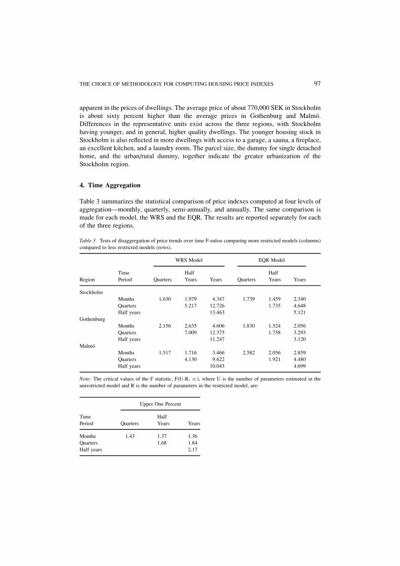
Table 3. Tests of disaggregation of price trends over time F-ratios comparing more restricted models (columns)

compared to less restricted models (rows).

WRS Model EQR Model

Time Half Half

Region Period Quarters Years Years Quarters Years Years

Stockholm

Months 1.630 1.979 4.347 1.739 1.459 2.340

Quarters 5.217 12.726 1.735 4.648

Half years 13.463 5.121

Gothenburg

Months 2.156 2.635 4.606 1.830 1.524 2.056

Quarters 7.009 12.375 1.758 3.293

Half years 11.247 3.120

MalmoÈ

Months 1.517 1.716 3.466 2.582 2.056 2.859

Quarters 4.130 9.622 1.921 4.480

Half years 10.043 4.699

Note: The critical values of the F statistic, F(U-R, ?), where U is the number of parameters estimated in the

unrestricted model and R is the number of parameters in the restricted model, are:

Upper One Percent

Time Half

Period Quarters Years Years

Months 1.43 1.37 1.36

Quarters 1.68 1.84

Half years 2.17


The table reports F-tests of the restrictions inherent in representing time in the

computation of price indexes by aggregate measures. For example, the entry in the ®rst

row and column provides a test of the hypothesis that, for the WRS model applied to data

from the Stockholm region, the coef®cients on monthly prices within quarters are

identical. According to the entry �F � 1:630�, the hypothesis can be rejected at the one

percent level of con®dence (where the critical value is 1.43).

The table presents a complete set of tests, comparing more restricted models (columns)

with less restricted models (rows) for all four aggregations of time initially measured in

days.5 The tests consistently allow rejection at the one percent level of the more

aggregated models against the less aggregated alternatives. These results hold across all

three regions both for a simple and parsimonious model, the WRS, and for a more

complete model, the EQR. The F-ratios are mostly larger for the WRS model than for the

EQR model, in particular when comparing the cruder levels of aggregation. The results for

the WRS model are quite consistent with those reported by CCM (1995, tables 1 through

5) for ®ve census regions in the U.S. The results reported in columns 4, 5, and 6 provide

further con®rmation, using a different model. The conclusion is clear: in the estimation of

housing price indexes, time should generally be represented using the lowest level of

aggregation possible. Arbitrary aggregations into broader representations of time are

generally unwarranted.

Table 4 indicates some of the implications of the aggregation of time in these three

bodies of data. Again we present estimates based on both the WRS and the EQR models

for different representations of time. The average values of the price indexes for the entire

period ( panel A) vary little with the representation of time, although there is a slight trend

upward as the level of aggregation increases. Furthermore, the estimated evolution of

nominal prices, including their acceleration beginning in 1986, their peak in 1991, and

their rapid decline thereafter, is consistent regardless of the degree of temporal

aggregation. This evolution is illustrated below. The mean values of the price indexes

for Stockholm and MalmoÈ are slightly higher for the WRS models than for the EQR

models, whereas the two models yield similar indexes for Gothenburg.

Panel B compares the estimated mean returns to investment in owner occupied housing,

for a one-year holding period. There is some tendency for returns estimates to be smaller

for larger aggregations of time. Further, the WRS models generally yield higher estimated

rates of return than the EQR models.

Panel C reports the estimated volatilities in annual returns implied by the various

models. The volatilities are computed from annual returns estimated using each model.

The estimated variance in annual returns is generally somewhat lower when estimated

from levels of time aggregation that are greater than monthly. The volatility is

substantially greater in Stockholm than in either Gothenburg or MalmoÈ.

5. Comparing Methodologies

Figures 1, 2, and 3 compare the estimates of the course of housing prices for the three

regions. The ®gures report the estimated price indexes as well as the 95% con®dence


intervals. All prices are estimated using the most appropriate representation of time, in

months. Results are presented for both methodologies, the WRS and the EQR methods.

Inspection of the ®gures reveals a striking regularity. While in each region the two

indexes track each other closely, the con®dence intervals are substantially narrower for the

Table 4. Estimates of house prices, returns, and volatilities.

WRS Models EQR Models

a. Mean Value of Price Index

(1981:Feb� 100)

Stockholm: Monthly 152.191 148.241

Quarterly 155.910 152.501

Semi-Annual 159.232 153.816

Annual 160.100 155.285

Gothenburg: Monthly 141.051 141.766

Quarterly 142.942 145.045

Semi-annual 146.256 145.284

Annual 147.703 145.731

MalmoÈ: Monthly 140.091 139.678

Quarterly 146.374 136.570

Semi-annual 146.749 138.990

Annual 149.508 140.837

b. Mean Return (times 100)

(Annualized percent change)


Quarterly 6.304 6.010

Semi-annual 6.081 5.806

Annual 5.973 5.759




Annual 5.641 5.429




Annual 6.420 5.453

c. Volatility (times 10000)

(Variance in annualized percent change)


Quarterly 138.084 147.200

Semi-annual 138.175 146.140

Annual 141.849 144.066


Quarterly 79.575 72.821


Annual 77.757 70.507


Quarterly 88.000 83.108


Annual 86.123 79.672


EQR models than for the WRS models. This is expected, as the EQR model incorporates

much more information in the estimation of the price index than does the WRS model. The

EQR model employs single sales as well as multiple sales, and it utilizes extensive

information about the qualitative and quantitative attributes of dwellings.

Figure 1.


The likelihood that an observed sale is a repeat sale increases with the length of the

sample periodÐthe samples used in the WRS and EQR methods should approach one

another as the time horizon is extended. During the thirteen year sample period, roughly

forty percent of observed sales are drawn from dwellings that sell at least two times.

Figure 2.


Table 5 shows how the repeat sales requirement greatly restricts the set of information on

which repeat sales indexes are based in short sample periods. The table also illustrates the

impact that this restriction has on the resulting con®dence intervals, as well as average

price levels and average percent returns.

Figure 3.


The table examines sample periods of various lengths for each of the three metropolitan

areas during segments of the price cycle that roughly correspond to stable, climbing, and

falling nominal house prices. Indexes are constructed using both the EQR and the WRS

methods for each of the sample periods. The relationship between length of sample period

Table 5. Differences between the EQR and WRS indexes as a function of sample period.

(Indexes are normalizedÐ1981: January� 100).

EQR Method WRS Method

Mean Mean

Percent Width of Mean Mean Width of Mean Mean

Repeat Con®dence Price Repeat Con®dence Price Percent

Sales Interval Level Return Interval Level Return

Stockholm:

1981±1982 4.6 7.441 96.328 ÿ 0.377 25.452 100.616 0.050

1983 8.0 6.927 96.770 ÿ 0.044 14.202 101.900 0.218

1984 11.9 7.236 97.478 0.077 12.777 100.911 0.213

1985 16.0 7.229 98.760 0.063 12.768 101.751 0.205

1986 19.6 6.808 100.803 0.283 11.236 103.511 0.313

1987±1988 3.4 10.732 118.123 1.296 28.921 118.464 1.434

1989 5.7 13.237 141.822 0.976 22.983 142.681 1.362

1991±1992 3.0 7.666 88.861 ÿ 1.690 35.844 91.999 ÿ 0.976

1993:Aug 4.5 7.901 84.550 ÿ 1.104 26.642 86.428 ÿ 0.616

Gothenburg:

1981±1982 7.4 7.384 98.704 ÿ 0.073 20.307 92.723 ÿ 0.129

1983 13.2 7.130 99.022 ÿ 0.011 15.388 96.769 0.160

1984 18.5 7.288 100.227 0.167 13.040 100.650 0.343

1985 21.6 7.329 101.965 0.178 12.346 101.594 0.253

1986 25.0 7.171 103.874 0.175 11.193 102.268 0.274

1987±1988 4.6 8.489 112.590 1.042 18.971 118.324 1.445

1989 7.5 9.672 122.825 0.845 17.390 124.269 1.365

1990 12.4 10.554 132.420 0.949 18.135 135.583 1.299

1991±1992 2.9 7.931 88.640 ÿ 1.083 22.239 93.651 ÿ 0.534

1993:Aug 4.4 8.561 86.061 ÿ 0.463 21.612 92.316 ÿ 0.029

MalmoÈ:

1981±1982 6.6 8.759 99.370 ÿ 0.098 24.925 92.471 0.219

1983 10.3 8.499 99.779 0.027 19.731 93.984 0.050

1984 13.7 8.124 100.629 0.126 16.585 98.502 0.269

1985 17.5 8.076 101.756 0.161 13.452 98.538 0.170

1986 21.6 8.488 102.965 0.168 12.239 99.861 0.212

1987±1988 5.6 8.827 106.987 0.912 20.509 108.231 0.862

1989 9.0 10.059 117.441 0.929 23.587 123.074 1.526

1990 14.6 11.079 127.704 0.993 18.502 135.710 1.288

1991±1992 4.3 9.767 93.275 ÿ 1.135 32.615 111.254 0.383

1993:Aug 6.1 10.711 90.445 ÿ 0.664 27.895 104.376 0.076


and percentage of observed sales which are repeat sales is as expected. It is clear that in

short sample periods indexes based on repeat sales utilize a very small fraction of the

available market information on housing sales. In Stockholm, the percentage of observed

sales that are drawn from dwellings that sell more than once rises from 4.6% to 19.6% as

the sample period increases from 24 to 72 months. The impact on the 95% con®dence

interval for the WRS index is striking, as the average width narrows from 25 to 11 units.

This noise in the price series has substantial impact on estimated average price levels

and estimated average returns. Both can vary widely between the two methods in short

intervals. However, there is a slight tendency for the differences to diminish as the sample

period is lengthened, and, as shown in table 4, the differences are small over the full

sample period. In Stockholm the difference between estimates of the average monthly

return during the initial 24-month period is close to half a percentage point. At the end of

the period of stable prices this difference is only 0.03 percentage points.

The advantage of the EQR method over the WRS method is obvious in these short

sample periods. In each case the con®dence interval for the indexes based on the EQR

method is substantially narrower. In the shortest intervals the intervals differ by a factor of

three. As expected, the difference declines as the sample period is lengthened and as the

percentage of sales which are repeat sales increases.

The small sample sizes that are used in a repeat sales index point to another potential

problem with their use. The repeat sales may not be a random sample of the housing stock.

(This, in turn, may bias estimates of price indices. See Englund, Quigley, and Redfearn,

1999). For example, ``starter'' homes are commonly thought to sell more frequently than

more expensive homes. As discussed above, over the course of the full sample period

approximately 40% of observed sales are drawn from units that sell more than once. This

percentage drops to under ten percent in shorter intervals. The data allow a comparison of

the populations used in the estimation of each index.

In general, the Swedish data support the notion that smaller, more modest homes sell

more frequently. However, as with the percentage of all sales that are second sales, the

average characteristics of dwellings must grow more similar as the sample period is

extended.6 In all three metropolitan areas, the average multiple sale unit in the short

sample periods is smaller, both in terms of interior and exterior size; it is less likely to be

detached, have a ®replace, or be on the waterfront. To the extent that price movements are

not identical across different populations of dwellings, a price index based on repeat sales

may be biased, in our case, tracking prices for smaller, more modest homes rather than the

price level for the entire housing stock.

That the percentage of observations drawn from dwellings which sell at least twice is so

small is particularly troubling in light of the implicit assumption about constant quality

between paired sales. As noted in the appendix, by basing the index upon the time interval

between sales of the ``same'' house (and only the time interval between sales), the

computation of the WRS index assumes that each house is really identical at each sale. The

WRS indexes constructed above are based on pairs of sales from the same dwelling

without regard to its underlying attributes. In order to employ the WRS method correctly,

those units that are altered between sales should be identi®ed and removed prior to

estimation of a WRS index, further reducing already small sample sizes. However, the


WRS method is often employed precisely because data on attributes are not available, thus

rendering veri®cation of the constant quality assumption impossible. The rich sample of

Swedish housing data permits this implicit assumption to be tested.

Table 6 identi®es the number and distribution of second sales over the course of the full

sample period. It also distinguishes between the total number of second sales and those

second sales that have remained unaltered across 26 measured characteristics. Panel B

reports that approximately forty percent of the second sales in the observed pairs have

been altered between sales.7 Of course, even if the measured characteristics of houses sold

at two points in time are the same, the dwellings are still not identical. The mere passage of

time means that the house may have depreciated.

As demonstrated in table 7, the changes in recorded housing quality between the ®rst

and second sale of each pair are generally consistent with improvements in housing quality

Table 6. Number and distribution of second sales.


A. Sales

Total number of sales 74077 106147 90741

Number of dwellings sold 12230 17683 16084

more than one time

Number of paired sales 14747 21450 19842

B. Paired Sales*

Identical Identical Identical

Years Paired Second Paired Second Paired Second

Between Sales Sales Sales Percent Sales Sales Percent Sales Sales Percent

0 928 779 83.9 2024 1479 73.1 1646 1293 78.6

1 2679 2177 81.3 4999 3777 75.6 4306 3288 76.4

2 2540 1900 74.8 4151 2881 69.4 3872 2790 72.1

3 2439 1547 63.4 3592 2173 60.5 3383 2009 59.4

4 1885 1027 54.5 2410 1281 53.2 2330 1311 56.3

5 1409 617 43.8 1647 782 47.5 1680 832 49.5

6 1070 381 35.6 1094 466 42.6 1135 474 41.8

7 833 231 27.7 707 251 35.5 692 232 33.5

8 478 85 17.8 408 100 24.5 429 82 19.1

9 274 27 9.9 259 46 17.8 220 29 13.2

10 146 19 13.0 113 14 12.4 116 15 12.9

11 55 5 9.1 39 7 18.0 33 5 15.2

12 11 1 9.1 7 4 57.1 0 0 0.0

Total 14747 8796 59.6 21450 13261 61.8 19842 12360 62.3

Note: *Number of paired sales, and the number of identical paired sales by interval between sales (using only

those observations for which no measured attributes have missing values)


over time. The availability of a garage, the quality of bathrooms and materials, and the

likelihood of a sauna and ®replace all increase. Several measures are not easily interpreted

as they have been affected by a rising standard (see note 8), but even for some of these

variables the average quality has improved between sales of dwellings. If these

improvements are ignored in the computation of the price index, the WRS will

overestimate housing price appreciation.

In addition, however, during the interval between sales, dwellings depreciate. Some or

all of this may be offset by expenditures on maintenance, but empirical evidence suggests

that the offset is incomplete (see Kain and Quigley, 1970, Palmquist, 1980, and Hill et al.,

1997, for examples using data obtained during three decades).

If unmeasured quality improvements of x percent are undertaken with probability peach year, while unmeasured depreciation net of normal maintenance is d percent, it is

easy to show that the price index ft computed from the WRS model will be a biased

estimate of the true price level, It.

E�ft� � It�1� pxÿ d�t: �1�

Figure 4 illustrates the dramatic difference between WRS indexes when the maintained

hypothesis of constant quality is enforced in one sample and explicitly violated in another.

Table 7. Changes in the attributes of the second sale of paired sales.

Percentage of units exhibiting changes in the level of an attribute.


Attribute Decrease Same Increase Decrease Same Increase Decrease Same Increase

Plot size 4.8 90.3 4.9 5.9 87.6 6.5 3.5 91.1 5.4

Living space 1.2 97.9 0.9 3.7 92.6 3.6 1.8 96.5 1.8

One-car garage 2.6 94.0 3.4 2.8 93.0 4.2 2.9 93.6 3.5

Two-car garage 1.0 98.6 0.4 0.9 98.0 1.1 0.7 98.4 0.9

Tiled bath 1.5 92.1 6.4 2.3 93.4 4.3 3.0 92.0 4.9

Sewer connection 0.1 99.6 0.3 0.2 98.9 0.9 0.1 99.1 0.8

Sauna 1.8 94.4 3.8 1.7 95.4 2.9 1.0 97.1 1.9

Wall construction 1.9 96.5 1.6 2.2 95.8 2.1 2.9 94.7 2.4

Furnished basement 2.6 95.3 2.2 2.1 95.4 2.5 1.1 97.2 1.7

Fireplace 0.9 96.4 2.7 2.0 94.1 4.0 1.0 95.0 4.0

Laundry room 4.7 92.0 3.3 4.8 91.4 3.8 4.7 91.1 4.1

Waterfront property 0.1 99.9 0.0 0.1 99.9 0.1 0.1 99.9 0.0

Quality 1a 3.8 94.3 1.8 4.2 93.1 2.7 3.5 94.1 2.4

Quality 2b 2.0 94.1 3.9 3.1 92.4 4.5 2.7 93.2 4.1

Good kitchen 5.7 89.7 4.6 5.8 88.8 5.4 6.4 87.7 5.9

Excellent kitchen 5.3 89.7 5.0 6.2 88.6 5.1 7.3 87.2 5.5

Heat 0.0 99.9 0.0 0.1 99.8 0.1 0.0 99.8 0.2

Good roof 0.2 99.3 0.5 0.2 99.1 0.7 0.2 98.9 0.9

Excellent Roof 0.9 96.2 2.9 1.6 95.7 2.7 2.2 94.3 3.5

Notes: Quality 1 is de®ned as ``winter quality''. Quality 2 is `ìsolation quality''.


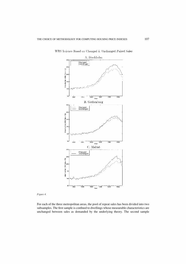
For each of the three metropolitan areas, the pool of repeat sales has been divided into two

subsamples. The ®rst sample is con®ned to dwellings whose measurable characteristics are

unchanged between sales as demanded by the underlying theory. The second sample

Figure 4.


consists of those pairs in which a change in attributes has been measured between sales.

The differences between the two indexes are clearly visible. Note that, despite the clear

difference in the evolution of prices, it is the union of these two data sets that serves as the

basis for repeat sales indexes that cannot differentiate between altered and unaltered

properties. In each of the three metropolitan areas the index that is based on altered

properties is substantially higher than the correctly estimated repeat sales index. This

difference is consistent with improvements in quality over time. Without measuring and

controlling for housing quality directly, the WRS methodology leads to much higher

estimates of housing prices during the second half of the sample period.

The indexes reported in ®gure 4 are based upon a sample which has ``®ltered out''

dwellings changed by explicit renovation decisions during the interval between sales. Of

necessity, however, the sample includes dwellings that have depreciated during the

interval. Thus, from equation (1), an index computed from this sample is lower than the

true price index.

The dilemma in computing the WRS index is clear: either ``®lter'' the data (to insure

that px � 0 for the houses used to compute the index) and thereby underestimate the price

index; or do not ``®lter'' the data and have no evidence at all about whether too much or

too little maintenance and improvement �px0d� has been performed.

Thus, a major advantage of the EQR methodology is the explicit measurement of

quality variation and differences in dwelling age over time.

6. Conclusion

In this paper, we have considered the aggregation of housing sales reported in continuous

time to discrete periods for the computation of indexes of house prices, investment returns,

and the volatility of returns. We have also considered the properties of repeat sales

estimators and hybrid estimators of the price indexes.

The analysis indicates quite clearly that house price estimates ought to be undertaken

using the ®nest disaggregation of time available. On statistical grounds, price indices

based on monthly aggregations dominate those based on quarterly data. Quarterly data, in

turn, dominates semi-annual data for the computation of price indices.8 In this conclusion,

we reinforce that made by Calhoun, Chinloy, and Megbolugbe using U.S. data. Volatilities

in returns are substantially higher when estimated using monthly time intervals. However,

our results also suggest that for a consistently de®ned holding period, returns and

volatilities do not differ very much, at least for this data set.

This analysis also suggests, however, that extreme caution should be exercised in

interpreting the WRS indices of housing prices as they are typically computed for

academic and business applications. The implicit assumption of constant quality is

dif®cult to verify, but is essential to the method. In the housing markets analyzed here,

dwelling improvements are undertaken frequently and are widespread. These changes in

physical structure violate the maintained hypothesis of the WRS method. Furthermore, the

results indicate that correctly implementing the WRS method greatly restricts the set of

observations that are utilized, perhaps narrowing the sample to observations drawn from


non-representative dwellings. In these conclusions, we reinforce those made by Meese and

Wallace (1997), using U.S. data which was more limited in geographical scope, sample

size, and in the measurement of housing prices. While further research is needed to clarify

the relationship between repeat sales indexes and price movements in the remainder of the

housing stock, it appears that the widespread use of the WRS indexes in the U.S. provides

an inadequate picture of housing price movements.

Appendix: Models of Housing Price Trends

1. The Weighted Repeat Sales Method

Assume, following Case and Shiller (1989), that the log price of the ith house at time t, Pit,

is given by

Pit � It � Hit � Nit (A1)

where It is the logarithm of the price level at t, Hit is a Gaussian random walk, such that

E�Hit ÿ Hit� � 0 (A2)

E�Hit ÿ Hit�2 � �tÿ t�sH2

and Nit is white noise, such that

E�Nit� � 0 (A3)

E�Nit�2 � sN2

Let Vit � Pit � Qit be the log sale price of house i at time t, where Qit is a quality indicator.

For houses sold at time t and time t (i.e., repeat sales) during the interval (1,S), the index is

computed in three steps. In the ®rst step, equation (A4) is estimated and the residuals, mit,

saved for use in the second step.

Vit ÿ Vit �X

s

fsDis � mit; s � �1; 2; . . . ; S�; (A4)

where Dis � 1 if s � t, Dis � ÿ1 if s � t, and Dis � 0 otherwise. fs is the estimate of Is,

the log of the price level at time s.

In the second stage, the squared residuals from (A4), �mit ÿ mit�2, are regressed upon a

constant and the elapsed time between sales, �tÿ t�, yielding estimates of the variances

sH2 and sN

2. In the third stage, equation (A4) is re-estimated by generalized least squares

with diagonal elements��s2

N � �tÿ t�s2H

p.


Note the assumption about dwelling quality implicit in this formulation. The left hand

side of (A4) can be interpreted unambiguously as a log price change if Qit � Qit. The

estimates of the price index are therefore functions of dwelling quality unless quality

remains constant across time. Clearly Qit � Qit is a maintained hypothesis in adopting this

procedure.

2. The Hybrid Method

Following Englund, Quigley, and Redfearn (1998), assume

Vit � bXit � Pit � xi � eit � bXit � Pit � git (A5)

where Xit represents the logarithm of observable characteristics of dwelling i, and Pit and

Vit are de®ned above. xi represents an error due to the unmeasured, individual-speci®c

characteristics of dwelling i and is distributed with zero mean and variance sx2. eit is an

error term. Components of Xit include the vintage �yi, year built� and the accumulated

depreciation �tÿ yi, age� of the dwelling. In a cross section, yi, �tÿ yi�, and Pt cannot be

separately identi®ed, but from a subsample of repeat sales at various ages and years, the

parameters can be recovered.

To implement the model, estimate (A5) using the subsample of paired repeat sales at

time t and time t. Then use the residuals from the regression to estimate jointly

git ÿ git � bd�tÿ t� � eit ÿ eit (A6)

and

eit � r�tÿt�ei;tÿt � Vit; (A7)

where ejt and ejt are de®ned as above, and r is the serial correlation coef®cient. Vit is the

residual, and is distributed with zero mean and variance sv2. Equation (A6) provides an

estimate of depreciation, bd.9

Together, these parameters yield an estimate of the variance-covariance matrix of the

errors in equation (A5). From equation (A7) we obtain an estimate of sv2. An estimate of

sx2 is constructed from the residuals in the ®rst-step estimation of (A5), knowing r and

sv2. Together these parameters describe completely the variance-covariance matrix of the

errors for equation (A7).

E�git; gjt� �0 for i 6� jsx

2 � sv2fr�tÿt�=�1ÿ r2�g � bd

2AtAt for i � j;

�(A8)

where Aj is the age of the house in year j.


The ®nal step is the re-estimation of (A5) by generalized least squares including all

observations in the sample, not merely repeat sales, and relying on equation (A8).

This hybrid method is more data intensive than the repeat sales method. It relies upon

qualitative and quantitative information about each housing unit at the time of sale to

control for housing quality in an explicit manner. The method also capitalizes on the

unique information provided by repeat sales of individual units. This permits us to separate

the effects of time on housing prices from depreciation and vintage effects and to improve

the ef®ciency of parameter estimates by explicit attention to the components of the error

structure.

Acknowledgments

Support for this research has been provided by the Fisher Center for Real Estate and Urban

Economics, University of California, Berkeley and by the Swedish Council for Building

Research. The paper has bene®ted from unusually constructive, detailed comments from

two anonymous reviewers.

Notes

1. This includes, for example, the price series marketed by Case-Shiller-Weiss, Inc., MRAC, and TRW, Inc.

2. ``Depreciation'' is the decline in quality over some time interval after accounting for normal maintenance,

while ``vintage'' refers to the elements of quality and style embedded in the dwelling at the time of

construction.

3. To insure that the observations included in the data were indeed arm's length market transactions, only the

®rst sale of paired sales that occurred within a six-month period were retained. This ®lter was imposed to

remove ``distressed sales'' and non-market transactions from the data set. Sales within the six-month period

were observed to have a large negative serial correlation. This is consistent with a distressed sale shortly after

an initial purchase or a pair of sales in which one serves as a familial transfer either preceded or followed by

an arm's length sale.

4. Beginning in 1975 the government provided interest-subsidized loans to owners of newly constructed

housing. The value of the subsidy depended on the construction costs and the vintage of the unit, and decayed

with time. While the average estimated present value of the subsidy (``capital subsidy'' in Table 2) is small,

less than 3000 SEK or $400 US, the average for transactions involving subsidized dwellings (``conditional

subsidy'' in Table 2) is an order of magnitude larger. During the 1980s the average subsidy on newly

constructed homes was as high as twenty percent of the initial price of the dwelling.

5. For each metropolitan region and for each model, the table presents tests of six joint null hypotheses, Hr;c0

where r is the row and c is the column. Without loss of generality, re-index the set of coef®cients f described

in Appendix A as fy:m where y is the year (1981 through 1993) and m is the month (1 through 12). For

convenience, we suppress the ®rst subscript. The six joint null hypotheses tested in the table are of the form:

H1;10 : f1 � f2 � f3 � fq1;f4 � f5 � f6 � fq2;f7 � f8 � f9 � fq3;f10 � f11 � f12 � fq4:

H1;20 : f1 � f2 � f3 � f4 � f5 � f6 � fh1;f7 � f8 � f9 � f10 � f11 � f12 � fh2:

H1;30 : f1 � f2 � f3 � f4 � f5 � f6 � f7 � f8 � f9 � f10 � f11 � f12 � fa1:

H2;20 : fq1 � fq2 � fh1;fq3 � fq4 � fh2:

H2;30 : fq1 � fq2 � fq3 � fq4 � fa1:

H3;30 : fh1 � fh2 � fa1:


6. Despite a time series of more than a dozen years, however, this convergence is slow in these data.

7. The only other study which compares paired sales with changes in attributes with paired sales of dwellings

with unchanged attributes, by Meese and Wallace (1997), uses data from Oakland and Fremont, California

over an 18 year period. For Oakland, Meese and Wallace found that 59% of paired sales had changes in the

measured attributes, while for Fremont, they reported that 47% of the dwellings had changed attributes.

8. As pointed out by a careful reviewer of this paper, these statements require some quali®cations. Our results

clearly reject the aggregation of temporal data from months to quarters to half-years to years in the

computation of housing price indexes. They do not provide evidence on the implications of aggregation for

the mean squared errors associated with the estimates. In both these respects, our results follow Calhoun, et

al. (1995). The more- and less-restrictive sets of estimates could be combined ef®ciently using a Bayes

estimator, but this is beyond the scope of the present paper. See Knight et al., (1992) for a description and a

relevant example.

9. Data on repeat sales allows the identi®cation of vintage, age, and depreciation effects. Subtracting the

estimate of the effect of depreciation obtained in equation (A8) from the coef®cient on the age estimated in

(A7) yields an estimate of the vintage effect. That is, bv � by ÿ bd .

References

Bailey, Marin J., Richard Muth, and Hugh O. Nourse. (1963). `À Regression Method for Real Estate Price Index

Construction,'' Journal of the American Statistical Association 4, 933±942.

Case, Karl E., and Robert J. Shiller. (1987). ``Prices of Single-Family Homes Since 1970: New Indexes from Four

Cities,'' New England Economic Review, 45±56.

Case, Karl E., and Robert J. Shiller. (1989). ``The Ef®ciency of the Market for Single Family Houses,'' AmericanEconomic Review 79, 125±137.

Calhoun, Charles A., Peter Chinloy, and Isaac Megbolugbe. (1995). ``Temporal Aggregation and House Price

Index Construction,'' Journal of Housing Research 6(3), 419±438.

Englund, Peter, John M. Quigley, and Christian L. Redfearn. (1998). `Ìmproved Price Indexes for Real Estate:

Measuring the Course of Swedish Housing Prices,'' Journal of Urban Economics, 44, 171±196.

Englund, Peter, John M. Quigley, and Christian L. Redfearn. (1999). Do Housing Transactions ProvideMisleading Evidence about the Course of House Values. Unpublished manuscript, University of California,

Berkeley, February.

Hill, R. Carter, John R. Knight, and C. F. Sirmans. (1997). `Èstimating Capital Asset Prices,'' Review ofEconomics and Statistics 79, 226±233.

Kain, John F., and John M. Quigley. (1970). ``Measuring the Value of Housing Quality,'' Journal of the AmericanStatistical Association, 532±548.

Knight, John R., R. Carter Hill, and C. F. Sirmans. (1992). ``Biased Prediction of House Values,'' The AREUEAJournal 20(3), 427±456.

Meese, Richard A., and Nancy F. Wallace. (1997). ``The Construction of Residential Housing Price Indices: A

Comparison of Repeat-Sales, Hedonic-Regression, and Hybrid Approaches,'' Journal of Real Estate Financeand Economics 14(1 & 2), 51±74.

Of®ce of Federal Housing Enterprise Oversight (OFHEO). (1997). 1997 Report to Congress. Washington, DC,

OFHEO.

Quigley, John M. (1995). `À Simple Hybrid Model for Estimating Real Estate Price Indices,'' Journal of HousingEconomics 4(1), 1±12.


Documents

The Choice of Methodology for Computing Housing Price Indexes: Comparisons …urbanpolicy.berkeley.edu/pdf/EQR_JREFE99.pdf · · 2002-04-03The Choice of Methodology for Computing