Embed Size (px)
Citation preview

DI
SC
US
SI
ON
P
AP
ER
S
ER
IE
S
Forschungsinstitut zur Zukunft der ArbeitInstitute for the Study of Labor
The Causal Effect of Retirement on Mortality:Evidence from Targeted Incentives to Retire Early
IZA DP No. 7570
August 2013
Hans BloemenStefan HochguertelJochem Zweerink

The Causal Effect of Retirement on Mortality:
Evidence from Targeted Incentives to Retire Early
Hans Bloemen VU University Amsterdam, Tinbergen Institute, Netspar and IZA
Stefan Hochguertel
VU University Amsterdam, Tinbergen Institute and Netspar
Jochem Zweerink VU University Amsterdam, Tinbergen Institute and Netspar
Discussion Paper No. 7570 August 2013
IZA
P.O. Box 7240 53072 Bonn
Germany
Phone: +49-228-3894-0 Fax: +49-228-3894-180
E-mail: [email protected]
Any opinions expressed here are those of the author(s) and not those of IZA. Research published in this series may include views on policy, but the institute itself takes no institutional policy positions. The IZA research network is committed to the IZA Guiding Principles of Research Integrity. The Institute for the Study of Labor (IZA) in Bonn is a local and virtual international research center and a place of communication between science, politics and business. IZA is an independent nonprofit organization supported by Deutsche Post Foundation. The center is associated with the University of Bonn and offers a stimulating research environment through its international network, workshops and conferences, data service, project support, research visits and doctoral program. IZA engages in (i) original and internationally competitive research in all fields of labor economics, (ii) development of policy concepts, and (iii) dissemination of research results and concepts to the interested public. IZA Discussion Papers often represent preliminary work and are circulated to encourage discussion. Citation of such a paper should account for its provisional character. A revised version may be available directly from the author.

IZA Discussion Paper No. 7570 August 2013
ABSTRACT
The Causal Effect of Retirement on Mortality: Evidence from Targeted Incentives to Retire Early*
This paper identifies and estimates the impact of early retirement on the probability to die within five years, using administrative micro panel data covering the entire population of the Netherlands. Among the older workers we focus on, a group of civil servants became eligible for retirement earlier than expected during a short time window. This exogenous policy change is used to instrument the retirement choice in a model that explains the probability to die within five years. Exploiting the panel structure of our data, we allow for unobserved heterogeneity by way of individual fixed effects in modeling the retirement choice and the probability to die. We find for men that early retirement, induced by the temporary decrease in the age of eligibility for retirement benefits, decreased the probability to die within five years by 2.5 percentage points. This is a strong effect. We find that our results are robust to several specification changes. JEL Classification: C26, I1, J26 Keywords: instruments, retirement, mortality Corresponding author: Jochem Zweerink, Department of Economics VU University Amsterdam Faculty of Economics and Business Administration De Boelelaan 1105 1081 HV Amsterdam The Netherlands E‐mail: [email protected]
* This paper is part of the Netspar research theme “Pensions, savings and retirement decisions (II),” subproject “Retirement decisions: financial incentives, wealth and flexibility”. We thank Maarten Lindeboom, David Neumark, Ola Vestad and seminar audiences at VU University Amsterdam, the IZA Workshop on Labor Markets and Labor Market Policies for Older Workers and the International Pension Workshop of Netspar for helpful and constructive comments.

1
1. Introduction
Understanding the nexus between life cycle labor supply, retirement, and morbidity and mortality is
of core interest to policy makers, given observed imbalances in current pension systems in the aging
societies of OECD countries. In pension systems that are of the defined benefit type, or that rely on
pay‐as‐you‐go social security, ceteris paribus, an increase (decrease) in effective retirement age
triggers either higher (lower) aggregate pension contributions or lower (higher) aggregate payouts, if
the system is to be held sustainable. The ceteris paribus clause in this statement is important,
however, as the discussion held in the academic literature on morbidity and mortality effects of the
retirement decision forcefully demonstrates. If longer working lives or later retirement lead to
adverse effects on health and even increase the likelihood of dying within a certain horizon, the
positive effect of increasing the normal retirement age on the sustainability of pensions is amplified.
We find evidence from the Netherlands that is consistent with such an adverse health or mortality
effect, albeit from a policy measure that reduced effective retirement age.
The policy change that we rely on became effective in 2005 for certain birth cohorts of civil servants
employed by the central government for more than ten years. These individuals were offered the
opportunity to retire during the year 2005, by a temporary reduction of the early retirement (ER)
eligibility age. According to our estimates, retirement led to a drop in the probability of men dying
within five years after retirement by 42.3 percent, or by 2.5 percentage points. This is a large and
significant effect. When we shift the horizon, we find the largest impact of retirement on survival
within the first year. Further analysis by primary cause of death suggests that one plausible
mechanism may work through the removal of stress‐related factors associated with demanding work
as we find significant effects on dying from a stroke.
Identifying the causal impact of retirement on morbidity or mortality is challenging, in particular as
the only research design that allows doing so has to rely on observational data on health and life
outcomes. The latter, in turn, calls for an approach that helps controlling the selection into
retirement since bad health typically triggers retirement and subsequently mortality. Our approach
uses the described policy variation as an instrument for retirement status in explaining the
probability of dying from both observable characteristics and unobservables. Importantly, we rely on
an individual fixed effects specification for the latter. We employ a difference‐in‐difference
specification on data for civil servants, controlling for year fixed effects and nonlinear age effects.
We use a difference‐in‐difference‐in‐difference specification for data on civil servants and workers
employed in other sectors. Our difference‐in‐difference‐in‐difference specification controls for year
2
fixed effects, nonlinear age effects and differences in year effects and nonlinear age effects between
civil servants and other workers. The probability to die within five years is the dependent variable in
our models. We choose the time horizon of five years since we are interested in the effect of early
retirement on mortality in the relatively short run. We do not want to estimate the effect of early
retirement on mortality in too short a run, because retirement may affect the probability to have
diseases that may lead to death within several years. The choice of evaluation horizon several years
ahead for the probability to die is limited by the time length of our panel data.
There is a range of related papers that investigate the effect of retirement on morbidity or health.
Papers that use age‐specific retirement rules provide very inconclusive findings, however. Charles
(2004), Hemingway et al. (2003), Coe and Lindeboom (2008), Neuman (2008), Coe and Zamarro
(2011), Blake and Garrouste (2012a, b) find that retirement has a positive impact on health.1 Kuhn et
al. (2010), Behncke (2012) and Dave et al. (2008) find a negative impact of retirement on health.2
What is not entirely understood in this literature is the way in which retirement changes morbidity
and mortality outcomes. In particular, direct evidence is scarce.
Our contribution to this literature is fourfold. First, our policy variation delivers a natural experiment
that we exploit to construct a strong and exogenous instrument. Becoming eligible for retirement
benefits due to the ER eligibility age for civil servants being reduced substantially increased the
probability to retire. Eligible civil servants only got to know about the decrease in the ER eligibility
age one year before they became eligible, so anticipation of early retirement can arguably be ruled
out. Second, we focus on mortality instead of health outcomes, an event which is distinctly and
objectively observed and does not raise issues of interpretation or subjectivity. Third, we use
administrative data covering the entire population, and thus follow a large number of individuals
over a number of years. As the mortality register essentially provides complete and measurement
error‐free information, we do not need to worry about selective attrition as an alternative reason for
not being recorded in the data anymore. Fourth, the unrivalled comprehensive database puts us in a
position to split the analysis by cause of death at a very detailed level and we can thus obtain
additional insights into the channels through which the positive effect of retirement on survival
(health) comes about.
1 Blake and Garrouste (2012b) use mortality as the outcome variable. They find a negative effect of later retirement on the probability to die within four years. 2 Kuhn et al. (2010) use mortality as the outcome variable. They find a positive effect of early retirement on the probability to die till age 67.
3
The rest of the paper is organized as follows. Section 2 reviews related literature. Section 3 describes
the institutional setting, including the policy shift decreasing the ER eligibility age. Section 4
discusses the data and provides insightful descriptives. Section 5 delineates the research design we
use to identify the causal effect of retirement on mortality outcomes, and Section 6 presents the
empirical results. Section 7 concludes.
2. Literature review
The theoretical impact of retirement on mortality is not clear‐cut. There are scores of papers in the
medical, gerontological and related disciplines that document heterogeneous patterns and
multifaceted potential pathways between retirement and health. Apart from physiological and
psychological processes that govern health, life style aspects are often discussed. Since individual
choices for both retirement and health behaviors reflect important trade‐offs that people face, we
think it is useful to start with briefly reviewing the main implications of the standard economic
approach.
Any discussion in the economic literature sees retirement as a one‐off, irreversible event. As
individuals with a poorer health are more likely to die than individuals with a better health, it seems
reasonable to assume that the impact of retirement on mortality runs through health. Early
retirement can have an impact on health through several mechanisms. Grossman (1972) provides a
framework for analyzing the causal relation between retirement and health. He models health as a
dual investment and consumption good. A healthy individual with fewer sick days is more productive
and more able to work than a less healthy individual. As health raises an individual’s productivity and
ability to work, the agent has an incentive to invest in his or her health. Health is also a consumption
good and directly features as an argument in the utility function. When the individual retires, costs
and benefits from health change. On the benefits side, the incentive to invest in health to raise
productivity and ability to work disappears after retirement.3 The utility that is derived from health
in a direct way may change after retirement. On the costs side, incentives to invest in health may be
different after retirement than before retirement. As an individual has more leisure time after
retirement, the time cost of investing in health is lower. As a result, an individual may, for instance,
physically exercise more frequently or go to the doctor sooner and be diagnosed and receive
3 Grossman does not consider productivity in household production. Individuals may value being productive in household production before and after retirement, giving an incentive to invest in health before and after retirement.

4
medical treatment when he or she has some physical or mental complaints.4 The sign of the net
effect of retirement on health in the Grossman model is unclear and depends on how retirement
changes the personal valuation of the costs of investment in health and the benefits from health
(Dave et al., 2008).
In empirical research, of course, health may act as a confounding variable. For instance, early studies
by Bazolli (1985) and Dwyer and Mitchell (1999) have found that health has a negative impact on the
probability to retire early. The literature on the impact of retirement on health addresses the
endogeneity of retirement status to health and mortality outcomes using a large range of different
identification strategies.5 Table 1 summarizes the literature. The focus in the literature has shifted in
recent years to studies that employ policy variation in order to measure the effect of interest in a
natural experiment setting. The definition of treatment and control groups remain context specific,
however. Charles (2004), Neuman (2008), Coe and Lindeboom (2008), Kuhn et al. (2010) and Blake
and Garrouste (2012a,b) instrument retirement status by retirement incentives that were age
and/or year specific. Coe and Zamarro (2011) and Behncke (2012) address the endogeneity of
retirement status by using institutions as an exogenous shifter of the probability to retire. Many of
these studies rely on subjective survey information from the U.S. Health and Retirement Study
(HRS).
Charles (2004) uses three sources of variation in the probability to retire to instrument retirement
status: age specific retirement incentives, a labor force participation enhancing change in the US
Social Security system and the elimination of mandatory retirement rules. Using HRS, Survey of Asset
and Health Dynamics among the Oldest Old (AHEAD) and National Longitudinal Survey of Mature
Men (NLS‐MM) data for men, the author finds that retirement has a positive impact on psychological
well‐being. Neuman (2008) uses age specific retirement incentives as an instrument for retirement
status. The author uses data from the HRS for men and women and finds that retirement improves
subjective health, although retirement does not affect physical functioning in daily activities, mental
health or the probability to have a chronic disease. The age specific retirement incentives used as an
4 Midanik et al. (1995) find that workers physically practice more once they retire. Boaz and Muller (1989) and Roos and Shapiro (1982) do not find evidence for workers receiving more ambulatory services from physicians once they retire. 5 The literature on the effect of retirement on health is closely related to the literature on the effect of job displacement on health. In that literature, job displacement is considered to be a stressful event, and the effect of job displacement on health or mortality is considered to run through stress. Sullivan and von Wachter (2009) find for data on older workers that job displacement has a strong and negative effect on mortality in the first year after job displacement. Browning et al. (2006) and Salm (2009) do not find an effect of job displacement on health.

5
instrument by Charles (2004) and Neuman (2008) concerned expected decreases in generosity of
retirement benefits for different age categories across time. The decreases in generosity of
retirement benefits have induced workers to postpone retirement. As the decreases in generosity of
retirement benefits were announced years ahead, workers may have anticipated them. Workers
who decided to postpone retirement because of the decreased generosity of retirement benefits
may have reduced the number of hours worked or may have started to live healthier, so that they
would have been better able to continue working. Anticipation may have biased the treatment
effect towards zero.
Coe and Lindeboom (2008) is an interesting paper since it addresses the endogeneity of retirement
status by using retirement windows as an instrument for retirement status. Early retirement
windows are incentives that promote retirement at a specific time. Employers determine to whom
these incentives are offered. We shall exploit a similar set‐up. With HRS data for men, Coe and
Lindeboom find that retirement increases self‐reported physical and mental health temporarily. The
authors also find that retirement improves health of highly educated workers. The authors find no
effect of retirement on mortality. As early retirement windows may be offered to workers with
certain health characteristics, the results may be biased.
Blake and Garrouste (2012a, b) use a policy change in France that provides incentives to retire and
affects specific birth cohorts of private sector workers as a source of exogenous variation in
retirement age. The authors use data on older workers from the 1999 and 2005 wave of the French
Baromètre Santé survey. Blake and Garrouste (2012a) estimate the treatment effect using two
methods. First, they use the reform as an instrument for retirement age. In their second approach,
the authors perform a before‐after difference‐in‐difference estimation. The control group consists of
public sector workers who are unaffected by the reform. The treatment group consists of private
sector workers who are affected by the reform. The instrumental variable and difference‐in‐
difference estimates indicate a positive impact of retirement age on physical and social health for
men and women. Blake and Garrouste (2012b) estimate the treatment effect employing an
instrumental variable approach and use data for men only. The authors use mortality within four
years as the outcome variable. They find that retiring one year later increases the probability to die
with 1.5 percentage points. This is equivalent to a decrease in life expectancy at age 64 by 1.68
months.
Kuhn et al. (2010) use a regional change in unemployment insurance (UI) rules in Austria as an
instrument for the difference between the statutory retirement age and the actual retirement age.
UI can be used in Austria as a pathway to (early) retirement. The change in UI rules allowed workers
6
in eligible regions to withdraw from the workforce up to 3.5 years earlier than those in non‐eligible
regions. Using administrative data for male and female blue‐collar workers, the authors find that for
every year a male worker retires earlier, the probability to die before age 67 increases by 2.4
percentages points or 13 percent. Hence, if a male worker retires 3.5 years earlier, the probability to
die before age 67 is increased by 8.4 percentage points or 46.9 percent. Especially cardiovascular
diseases are found to be responsible for the increase in the probability to die. One of the plausible
channels that emerges from the analysis is that alcohol use and also smoking change upon
retirement and eventually cause ill health. The authors do not find an effect of early retirement on
mortality for female workers.
Coe and Zamarro (2011) employ a fuzzy regression discontinuity design, using the eligibility age for
public old‐age benefits as the point of discontinuity in the probability to retire. The authors use
single cross‐section data from eleven European countries for men only. The data are collected in the
Survey of Health, Aging and Retirement in Europe (SHARE). The authors find a positive impact of
retirement on general health for workers aged 65. The authors do not find an effect for workers
younger than age 65. Behncke (2012) exploits the eligibility age for public old‐age pension benefits
as a source of exogenous variation in retirement status. The author employs propensity score
matching as well as an instrumental variable approach. For propensity score matching, workers who
reached the eligibility age for public old‐age pension benefits are matched to similar workers who
did not reach the eligibility age for public old‐age pension benefits yet. For the instrumental variable
approach, the author uses the eligibility age for public old‐age pension benefits as an instrument for
retirement status. Behncke controls for anticipation of retirement by adding expectations about
future work and health as control variables in her analyses. Using data from the English Longitudinal
Study of Ageing (ELSA), the author finds that retirement increases the probability of being diagnosed
with a chronic condition such as a heart disease or cancer for men and women.
Hemingway et al. (2003) and Dave et al. (2008) use alternative approaches to address the
endogeneity of retirement status. Dave et al. (2008) try to limit the endogeneity bias by only
considering workers who were healthy before retirement. They estimate models in which retirement
status and health status are mutually dependent. The authors use data from the HRS and AHEAD.
They find that retirement induces a six percent increase in illnesses and a six to nine percent
increase in depressions for men and women. Hemingway et al. (2003) estimate the impact of
retirement on health, using data for male and female civil servants from the Whitehall II study. Some
particular groups of civil servants were allowed to retire later than the regular mandatory retirement
age. The authors compare changes in health of unaffected civil servants retiring at the mandatory

7
retirement age with those of affected civil servants retiring later. Important here is that cases of ill‐
health retirement are excluded from the sample. The authors find no effect of retirement on
physical health for men and women and a positive effect of retirement on mental health for men
and women in higher socioeconomic status groups.
3. Institutional background and policy change
We follow the recent literature that exploits quasi‐experimental variation afforded by changes in
retirement rules. In particular, we shall focus on targeted incentives to retire early that became
available to a group of civil servants in the Netherlands. The Dutch retirement system foresees in
retirement at the standard age (for both men and women) of 65. Actual average ages of entering
retirement have been considerably lower, however, due to the widespread use of early retirement
arrangements in virtually all sectors of the economy. 6
The Dutch pension system rests on three pillars (Bovenberg and Meijdam, 2001). The first pillar is
the public old‐age pension, which is financed on a pay‐as‐you‐go basis. The second pillar consists of
occupational pensions, which are funded. The third pillar consists of private provisions. We study the
period around 2005. At that time most occupational pension funds offered early retirement
arrangements. The public sector pension fund offered arrangements for early retirement as of the
ages 61 or 62 onwards. We use a temporary decrease in the ER eligibility age for civil servants as a
source of exogenous variation to estimate the impact of early retirement on the probability to die
within five years.
In April 2004, a temporary decrease in ER eligibility age for civil servants was announced. We refer to
the temporary decrease in the ER eligibility age for civil servants as `the early retirement
arrangement’ in the sequel. Due to a reorganization of the central government, employers being
part of the central government were allowed to offer certain civil servants additional possibilities for
early retirement in the year 2005. Employers were only allowed to offer early retirement if this
would prevent the forced layoff of another civil servant.7 The early retirement arrangement offered
gross retirement benefits that could be up to 70 percent of workers’ final wage, which corresponds
to the benefit level in other ER programs.8
6 A description of the Dutch pension system and existing early retirement arrangements for civil servants can be found in the appendix of this paper. 7 Forced layoff refers to forced layoff due to reorganization. 8 The replacement rate depended among others on the birth date of an individual.

8
Civil servants faced several eligibility criteria for participation in the early retirement arrangement.
First, they had to be at least 55 at the moment of early retirement. Second, they needed to have
been employed as a civil servants continuously during the ten years prior to early retirement. This
requirement is of importance for our study, as it prevents self‐selection of workers who would like to
retire early into the public sector. Civil servants were required to have contributed to the public
sector pension fund continuously during the ten years prior to early retirement.9 Employers were
allowed to offer participation in the early retirement arrangement until 1 January 2005 and
participating civil servants were not allowed to retire later than 1 December 2005. Participating civil
servants were entitled to early retirement benefits until age 65 with a maximum duration of eight
years. Civil servants aged 57 or older at the moment of early retirement were thus entitled to
retirement benefits for the whole period until normal retirement at age 65. Civil servants born
before 1 January 1948 could continue accruing pension claims at a rate of 50 percent at the expense
of the employer for a maximum of four years. Civil servants born on or later than 1 January 1948, i.e.
civil servants who were aged 55‐57 in 2005, did not have this opportunity. The early retirement
arrangement was thus very attractive for civil servants aged 58 and older,10 less attractive for civil
servants aged 57 and even less attractive for civil servants aged 55 or 56.
4. Data
We use Dutch administrative data for the period 1999‐2010. The data are administered by Statistics
Netherlands. We have access to data on mortality, hospital stays, and job and personal
characteristics originating from various administrative sources that can be linked with a personal
identifier.11 12 The mortality file provides information such as year and primary (and secondary)
cause(s) of death. The hospital stay file provides for every hospital stay information such as the start
and end date of the stay, the reason for the stay and where the patient went after being released
from the hospital. The job characteristics file provides information on all jobs any individual has been
9 Interruption of employment and pension contribution of at most two months was allowed, although interruption of employment and pension contribution in the half year prior to early retirement would have led to loss of eligibility. 10 The offer of early retirement through the particular ER window was “an offer they could not refuse” for this group of individuals. 11 The original file names are Doodsoorzaken (1999‐2010), Landelijke Medische Registratie (LMR, 1998‐2004), SSB Banen (1999‐2008), SSB Personen (1999‐2005) and PARTNERBUS (2010). 12 Statistics Netherlands only provides data that are administered by governmental institutions. These data provide only limited information. Moreover, the data that are administered are not always administered for the years we are interested in. Data on financial wealth, for instance, are not available for the years of study. Hospital stays data are incomplete after 2005, so that it is not possible to estimate the effect of early retirement on alternative health measures created from hospital data.

9
employed in during 1999‐2005. For every job, both start and end date, the industry code and the
annual wage are available.13 The personal characteristics file contains information on demographic
characteristics such as nationality, marital status, birth year and birth month. The personal
characteristics file also includes a partner identifier that allows us to link partners to each other. The
files we use cover all residents registered with Dutch municipalities.
For our analysis we select observations on individuals aged 53‐60 during 1999‐2005. We exclude
observations on individuals without a Dutch citizenship during 1999‐2005. We also exclude
observations for which the relevant individual has not been continuously employed for the ten years
prior to January 1st of the year of observation. We make this selection, as one of the eligibility
criteria for participation in the early retirement arrangement for civil servants is that civil servants
have been continuously employed as a civil servant for the ten years prior to early retirement. For
the same reasons, observations on workers who switched between the public sector and any other
sector are excluded from the analysis as well. Observations on workers who stayed in the hospital
somewhere between 1998 and retirement are also excluded from our analysis.14 By dropping the
observations on workers who stayed in the hospital before retirement, we aim to limit the
endogeneity of retirement status to health. We also drop observations for the years after the year
in which a worker has retired.15 We use about 155,000 observations on male civil servants and about
34,000 observations on female civil servants.
Table 2 shows descriptive statistics for civil servants and workers employed outside the public
sector. Age is measured on December 31st of the respective year. The variable married takes value 1
if a worker had a partner in the year of observation, 0 otherwise.16 Lagged wage income indicates
the total wage income a worker earned in the year prior to the year of observation. Lagged wage
income is measured in thousands of deflated Euros. We only have a limited number of variables at
our disposal that we can use as controls. Because of this, the individual fixed effects that we control
for in our instrumental variable model are expected to be important in explaining retirement status
and the probability to die within five years. One might think in the first place of effects due to year of
birth, education, or chronic health conditions. In addition, the fixed effects also correct for time‐
13 The industry code for the central government is 7511 according to the Standaard Bedrijfsindeling 1993 (SBI ‘93) classification. 14 If a worker was hospitalized but did not retire in 1999‐2005, all observations on this worker are dropped. 15 We assume that individuals do not work after retirement, though we can only observe employment state until January 1st, 2009. This is discussed in more detail later in this section. 16 Having a partner includes being married and having a registered partnership, but excludes cohabitation without being married or without having a registered partnership. Registered partnership refers to partnerships enjoying legal status similar to marriage.

10
constant heterogeneity that remains unobserved in administrative data, such as preference
parameters determining choices.
The average age of individuals in our dataset is 56, which indicates that relatively young individuals
are relatively overrepresented in our dataset.17 Male civil servants are in general comparable to male
workers employed in other sectors. Female civil servants clearly differ from female workers
employed outside the public sector. Wage income in the year prior to the year of observation was
higher for female civil servants than for female workers employed outside the public sector.
Moreover, female civil servants had a lower probability to have a partner than women employed
outside the public sector. Table 2 also shows that the control group is similar in marital status and
lagged wage income to the treatment group. The control group includes civil servants aged 53‐54 in
2005, i.e. those civil servants who could not be offered early retirement. The treatment group
includes civil servants aged 55‐60 in 2005, i.e. those civil servants who could be offered early
retirement. Differences in marital status and lagged wage income between workers in the control
group and those of the same age employed in other sectors are similar to those between workers in
the treatment group and those of the same age employed in other sectors.
The group of civil servants that could be offered early retirement due to the temporary decrease in
the ER eligibility age consisted of civil servants working for the central government. The sector in
which individuals work is identified by an industry code. Most civil servants working for the central
government were assigned the same industry code as some groups of civil servants who were not
working for the central government. Hence, we cannot precisely identify the group of civil servants
working for the central government. When we refer to civil servants later on in this paper, it should
be kept in mind that we mean central government civil servants including a group of other civil
servants who were ineligible for the early retirement arrangement of interest.18 Another data issue
is that we do not observe to which civil servants early retirement was offered. We can thus not
observe whether an eligible civil servant rejected the early retirement offer or whether a civil
servant with characteristics of an eligible civil servant did not retire early because he or she was not
offered the early retirement arrangement. Thus, the “treatment” group we define in our data is
somewhat wider than the “true” treatment group.19 We also do not know whether there was
selection in offering the early retirement arrangement to some specific groups only, e.g. to workers
17 This is partly the result of dropping observations after having transitioned into retirement. 18 This issue may lead to our estimates of the impact of the early retirement arrangement on retirement constituting lower bounds of the real impact, and likewise to possible bias of the estimates of the impact of early retirement on the probability to die within five years towards zero. 19 We do not know how much larger the treatment group is than the “true” treatment group.

11
who were relatively less productive or were relatively often ill. If there would have been selection,
this could bias our results or could at least force us to reinterpret our results. The final data issue
concerns the absence of information on whether individuals receive retirement benefits. We define
retirement as having exited a job and not having started working again before January 1st, 2009.
Figures 1a and 1b show that the probability that male and female civil servants die within five years
increases across age for several birth cohorts. There are birth cohorts that follow different patterns
as well. Civil servants who were born relatively long ago have in general a higher probability to die
within five years than civil servants with the same age who were born relatively recently. The
observed patterns are not smooth and do not show consistent patterns for all birth cohorts.20 We
consult mortality data on the whole population from Statistics Netherlands to get a better view on
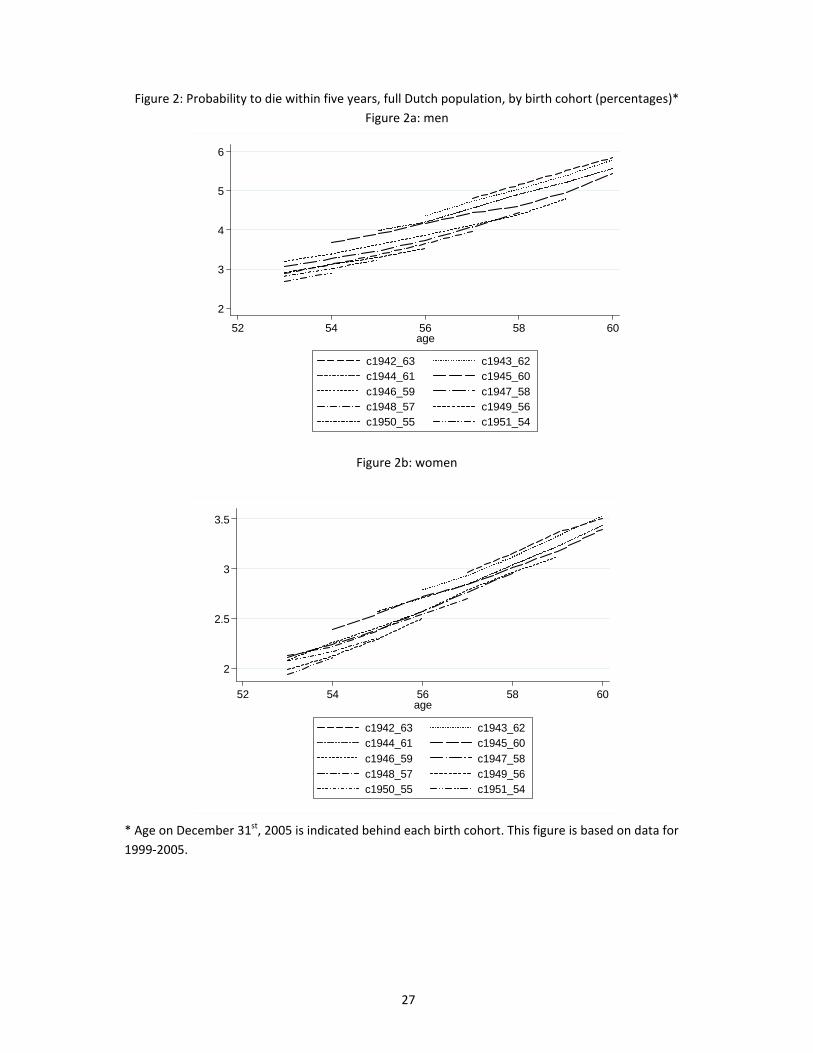
mortality patterns across age and birth cohorts. Figures 2a and 2b show that the probability to die
within five years for the whole Dutch population increases smoothly across age and decreases
smoothly across birth cohorts.21 Observed probabilities are higher than those observed for civil
servants. This is intuitive, as individuals employed as a civil servant may have a relatively modest
probability to die within five years compared to, for instance, individuals who do not work. The
probabilities to die within five years are higher for men than for women. The age gradient in the
probability to die within five years is higher for men than for women as well.
5. Methodology
We employ an instrumental variable approach to estimate the impact of early retirement on the
probability to die within five years. We instrument the retirement choice by dummies for the ages
for which civil servants are eligible for the early retirement arrangement interacted with a dummy
for the year of the policy change and a dummy for being a civil servant. We estimate a model using a
difference‐in‐difference specification for civil servants and a model using a difference‐in‐difference‐
in‐difference specification for civil servants and workers employed outside the public sector. In the
model using the difference‐in‐difference specification, the source of exogenous variation in
retirement status is the age in 2005.22 In the model using the difference‐in‐difference‐in‐difference
specification, being or not being a civil servant in 2005 is the additional source of exogenous
variation. Being or not being a civil servant is exogenous here, because we only include observations
where the relevant individual has been either continuously employed as a civil servant for the ten
20 This is in combination with the probabilities to die within five years being low. 21 The cohort of individuals born in 1945 shows a slightly deviating pattern for the ages 53‐57. 22 Age in 2005 determines eligibility for the ER arrangement, see Section 3.

12
years prior to the year of observation or continuously employed outside the public sector for the ten
years prior to the year of observation.
We use civil servants aged 53 or 54 in 2005 as the control group and civil servants aged 55‐60 in
2005 as the treatment group. 23 Our models control for individual fixed effects. As men and women
have different retirement patterns and remaining life expectancies, we estimate our model for men
and women separately. The treatment effect we estimate is the Local Average Treatment Effect
(LATE), i.e. the effect of early retirement on the probability to die within five years for those who are
induced to retire early by variation in the instruments.
5.1 Instrument validity
The instrument we use is valid if two conditions are satisfied. First, the instrument has an impact on
the probability that individuals receive the treatment. Second, the instrument does not correlate
with unobserved factors having an impact on the outcome. The instruments we use are dummies for
eligibility for retirement benefits due to the temporary decrease in the ER eligibility age for civil
servants in 2005.
Figures 3a and 3b show retirement rates for male and female civil servants. Retirement rates for civil
servants aged 58‐60 were substantially higher in 2005 than in other years. Retirement rates for civil
servants aged 56‐57 and female civil servants aged 55 were higher in 2005 than in other years as
well. Retirement rates for civil servants aged 53 and 54 were similar in 2005 as in other years. This is
in line with the incentives provided by the introduction of the early retirement arrangement and
suggests that the early retirement arrangement for civil servants induced civil servants to retire
early.24
We do not have reasons to expect that the introduction of the early retirement arrangement had a
direct impact on the probability to die within five years. To our knowledge, there were no events in
2005 or in the five years after that shocked the probability to die within five years for civil servants
aged 55‐60 in 2005 particularly, other than the reform we study. We also do not have reasons to
expect that our instruments are correlated with unobserved factors that influenced the probability
23 As we estimate a fixed effects model, observations on individuals that we observe for only one year are not used. As civil servants aged 53 in 2005 are observed for only one year, observations on these civil servants are not used. This implies that our control group consists only of civil servants aged 54 in 2005. 24 There were several other pension related policy changes around the period under review. These policy changes and their possible effects on retirement rates are discussed in the Appendix.

13
to die within five years. Unobserved factors that are expected to have influenced the probability to
die within five years may include the unobserved level of health, health‐related behavior,25 the
number of hours worked and associated stress levels. If retirement induced by the early retirement
arrangement was anticipated, the number of hours worked and health‐related behavior may have
been correlated with the introduction of the early retirement arrangement. However, the
introduction of the early retirement was only announced in April 2004 and employers decided only
later in 2004 whether they would offer a civil servant the early retirement arrangement. As civil
servants were only informed late during 2004 whether they were offered the early retirement
arrangement, we do not expect anticipation of early retirement to be an issue. Another possible
concern is that the jump in retirement rates for civil servants in 2005 is driven by factors other than
the introduction of the early retirement arrangement for civil servants in 2005. Figures 4a and 4b
show that retirement rates for workers aged 55‐60 employed outside the public sector were not
higher in 2005 than in other years. This indicates that the difference in retirement rates for civil
servants aged 55‐60 between 2005 and other years is not caused by factors that shifted retirement
rates of the entire workforce in 2005.
The validity of the difference‐in‐difference‐in‐difference approach depends on the justification of the
common trend assumption. The common trend assumption implies that the probability to die within
five years and the probability to retire for civil servants follow trends similar to those of workers
employed outside the public sector. Figures 5a and 5b show that the probabilities to die within five
years for workers employed outside the public sector follow similar patterns as those for civil
servants for only several birth cohorts. We have discussed above that retirement rates of civil
servants aged 59 or younger follow similar patterns as those of workers employed outside the public
sector. As the patterns for the probability to die within five years across age for civil servants differ
from those for workers employed in other sectors, the common trend assumption is possibly
violated. Nevertheless, the approach is valuable, as it provides estimates based on imposing a rather
smooth probability to die within five years across age patterns on civil servants.
5.2 Model specification
We estimate the LATE using a two‐stage‐least‐squares fixed effects instrumental variable model. In
the first stage, retirement status is estimated and in the second stage, the impact of predicted
retirement on the probability to die within five years is estimated. Our instrumental variable model
has as advantage that it controls for time‐invariant unobserved heterogeneity and allows the
25 Including getting diagnosed and treated.

14
individual fixed effects to be correlated with observed characteristics. We use a difference‐in‐
difference specification for our model and estimate it for civil servants only. We control for year
effects and for differences in the probability to die within five years and the probability to retire
across age. The first stage of the difference‐in‐difference variant of our model is specified as follows:
(1) ∑ ∑ ∑ , ,
where is a dummy that is 1 if individual i is aged 55 or older in year t and individual i retired in
year t. is 0 otherwise. is a year dummy that is 1 in year j and 0 otherwise. denotes the
difference between the age of individual i in year t and 53, taken to the kth power.26 is an age
dummy that is 1 if individual i reaches age l in year t and 0 otherwise. is a dummy that is 1 if
individual i has a partner in year t and 0 otherwise. includes lagged wage income. is an
individual fixed effect. is an error term. is allowed to be correlated with all covariates.
The second stage is specified as follows:
(2) ∑ ∑
where is a dummy that is 1 if individual i dies within five years after year t and 0 otherwise.
indicates the LATE. is allowed to be correlated with all covariates. and are also allowed to be
correlated. and are allowed to be correlated as well.
We also estimate the LATE using a difference‐in‐difference‐in‐difference specification for data on
civil servants and workers employed outside the public sector. We do so, because the retirement
and mortality patterns of workers employed outside the public sector, shown in Figures 4 and 5, are
smoother than those for civil servants shown in Figures 1 and 3. This is due to the relatively modest
number of observations for civil servants. The first stage of the instrumental variable model for the
entire workforce is specified as follows:
(3) ∑ ∑ ∑ , , ∑
, ∑ ∑ , ,
where is a dummy that is 1 if individual i is a civil servant in year t and 0 otherwise. is a
dummy that is 1 if individual i works outside the public sector in year t and 0 otherwise. The
difference between (3) and (1) is the inclusion of the interactions between the age variables and the
dummy for being a civil servant, the interactions between year dummies and the dummy for being a
26 We do not include in our models. Including is not possible due to multicollinearity caused by the presence of the year dummies.

15
civil servant, and the interaction between the dummy for 2005 and the dummy for not being a civil
servant. Moreover, the instruments in (1), i.e. the interactions between the dummy for 2005 and the
age dummies, are interacted with the dummy for being a civil servant in (3). As the difference‐in‐
difference specification does, the difference‐in‐difference‐in‐difference specification controls for
nonlinear age effects and year fixed effects. In addition, the difference‐in‐difference‐in‐difference
specification controls for differences in nonlinear age effects and year fixed effects between civil
servants and workers employed outside the public sector.
The second stage of the instrumental variable model for the entire workforce is specified as follows:
(4) ∑ ∑ ∑ ∑
,
The differences between (4) and (2) are essentially the same as those between (3) and (1).
6. Results
6.1 The uninstrumented case
We instrument retirement status because of the potential endogeneity of retirement status to
health. Table 3 shows the difference‐in‐difference and difference‐in‐difference‐in‐difference
estimates with individual fixed effects for when retirement is not instrumented, i.e. the estimates of
in (2) and (4) with retirement status instead of predicted retirement status . The coefficient
estimates on retirement are positive and significant at the five percent level for men. The difference‐
in‐difference‐in‐difference coefficient estimate for women is positive and significant as well. The
difference‐in‐difference coefficient estimate for women is not significant. For men, the difference‐in‐
difference coefficient estimate indicates that retirement is associated with a 0.6 percentage point, or
16.7 percent, higher probability to die within five years. The difference‐in‐difference‐in‐difference
estimate for men is 0.4 percentage point, or 9 percent, and for women 0.1 percentage point, or 6.1
percent respectively. If retirement status would not be endogenous to health, we would expect the
coefficient estimate on retirement status in these uninstrumented fixed effects models to be similar
to those of the instrumental variable models with fixed effects.

16
6.2 Instrumental variable estimates
Table 4 shows the instrumental variable fixed effects estimates using the difference‐in‐difference
and difference‐in‐difference‐in‐difference specifications.27 The estimates using the difference‐in‐
difference specification show that retirement induced by the early retirement arrangement
decreased the probability to die within five years by 2.5 percentage points, or 42.3 percent, for men.
Blake and Garrouste (2012b) find effects of a similar order of magnitude. Kuhn et al. (2010) also find
large effects for blue‐collar workers, however of the opposite sign. This suggests that the absolute
magnitude of the effect we find is not particularly striking. The LATE for women is not significant at
the ten percent level. The difference‐in‐difference‐in‐difference instrumental variable estimates are
very similar to the difference‐in‐difference instrumental variables estimates.
The F statistics for the relevance of the instruments in the first stage show that our instruments are
relevant at the one percent significance level. The coefficients on the instruments in the first stage
are positive, indicating that the introduction of the early retirement arrangement did induce eligible
civil servants to retire. The J statistics for exogeneity of our instruments show that the null
hypothesis that our instruments are exogenous cannot be rejected at the ten percent significance
level for men. However, the J statistics show that instruments suffer from endogeneity for women.28
We can thus not interpret the LATE estimate for women as a causal effect.
6.3 Causes of death
Specific causes of death may be related to working or being retired. For instance, if working would
impose a high risk on accidents, the effect of retirement on mortality may run through accidents.
This mechanism would then be revealed by considering mortality due to accidents. To get more
insight into the mechanism through which early retirement affects mortality, we estimate the
instrumental variable models in (1)‐(2) and (3)‐(4) using a dummy for dying within five years due to a
specific cause as a dependent variable. The causes of death for which we estimate our models are
grouped according to the 10th Revision of the International Statistical Classification of Diseases and
Related Health Problems (ICD). The ICD is a health care classification system by the World Health
Organization (WHO, 2010). The ICD provides diagnostic codes for classifying diseases. The diseases
27 The probability to die within five years is negative in lagged wage income, positive in lagged health and positive in age. 28 The rejection of the null hypothesis that the instruments are exogenous is probably the result of the small number of observations for female civil servants. As the number of civil servants retiring in 2005 and die within five years after 2005 is small, fatalities unrelated to retirement can easily threaten the exogeneity of the instruments.

17
are grouped into 22 categories, so called chapters. We estimate the causes of death for the
chapters, or, in case of the frequent causes of death cancer and diseases of the circulatory system,
subchapters, so called blocks. Chapters counting less than ten observations on fatalities are merged
in the category “Other diseases”.
Tables 5 and 6 show that the LATEs of early retirement on mortality due to almost all causes of
death are negative. This indicates that the effect of early retirement on mortality does not run
mainly through a particular cause of death, but rather through many causes of death. Most LATEs
are not significant. This is due to the small number of fatalities due to specific causes of death. The
LATEs of early retirement on mortality due to stroke (cerebrovascular diseases), liver diseases
(diseases of the digestive system) and accidents (external causes of morbidity and mortality) are
exceptions. They are negative and significant at successively the one, one and ten percent level.
Early retirement has a negative LATE of 0.5 percentage point or 12.7 percent on the probability to
die within five years due to stroke. This implies that there are 11 fatalities due to stroke less within
five years because workers were induced to retire by the early retirement arrangement. This is a
large number as there were only 2,348 workers induced to retire early. Stroke as a cause of death is
interesting in the context of this paper, since life style can have a significant impact on the
probability of dying from stroke. Hypertension, diabetes, obesity, alcohol use, smoking and lack of
physical exercise are among the modifiable risk factors for stroke.29 Hypertension is the most
important modifiable risk factor for stroke. Risk factors for hypertension include obesity, smoking,
alcohol consumption and lack of physical exercise (Appel et al., 2006, Begg et al., 2006), so obesity
and smoking pose a direct and indirect threat for contracting stroke. Stress may result in
hypertension as well (Kaplan and Nunes, 2003).
6.4 Distribution of treatment effects across time horizons
We have estimated the effect of early retirement induced by the introduction of an early retirement
arrangement on the probability to die within five years. Table 7 shows the estimates for the effect of
early retirement on the probability to die within fewer years. Though insignificant at the five percent
level, the coefficient on the effect of early retirement on the probability to die within one year is
large and negative in size. Differences between the effect of early retirement on the probability to
die within one and two, two and three, and three and four years are positive and relatively modest
in size. This indicates that the effect of early retirement on dying during each of the second to fourth
29 Risk factor indicates a factor that is correlated with the prevalence of a disease. There is not necessarily a causal relation between a risk factor and the prevalence of a disease.
18
year are negative and relatively modest in size compared to the effect of early retirement on dying
during the first year after retirement. Hemmingway et al. (2003) provide a possible explanation of
the relatively large effect of early retirement on the probability to die during the first year after
retirement. They suggest that retirement may improve health as it takes away the demand from
work and stress of work. In our case, the disappearance of demand from work and stress of work
may have had a positive effect on health instantly. The immediate positive effect on health may have
translated into a negative effect on the probability to die within one year. The difference between
the effect of early retirement on dying within four years and the effect of early retirement on dying
within five years is even negative, indicating that early retirement has a positive impact on the
probability to die during the fifth year. We may expect the probability to die during the years
following the fifth year to be positive as well. The reason for this is that since all considered workers
will die eventually, irrespective of whether they retire or not, the effect of early retirement on the
probability to die in, say, a hundred years, is zero. Because of workers’ mortality, we expect the
impact of early retirement on mortality to die out when the time horizon for the probability to die is
lengthened. This may explain why the effect of early retirement on the probability to die during the
fifth year is positive, though the effect of early retirement on the probability to die during the
previous years is negative.
6.5 Robustness checks
Our statements concerning the probability to die within five years are to be understood conditional
on age. Age is an important determinant of both retirement status and the probability to die within
five years. This may make our results sensitive to the way age enters our models. We control for
second and third order age effects in our instrumental variable model. This baseline estimate is
redisplayed as variation a in Table 8. As a robustness check, we estimate the difference‐in‐difference
instrumental variable model once controlling for second order age effects only and once controlling
for second, third and fourth order age effects. We perform a similar robustness check for the
difference‐in‐difference‐in‐difference instrumental variable model. Table 8 shows that the LATE
estimates for the alternative models are similar to the LATE estimates for the models we use. This
indicates that our instrumental variable results are robust to controlling for age effects of one order
lower or one order higher (variations b and c).
Married men may make retirement decisions in a different way than single men. Married men may,
for instance, take into account whether their spouse is retired or whether there are grandchildren
present that need attention. As marital status may affect lifestyle, the probability to die within five

19
years may also be affected. This may induce the coefficients on, for instance age, in the first and
second stage of the instrumental variable models to be different for married men than for single
men. We verify whether differences in coefficients between married men and unmarried men affect
our LATE estimates. Table 8, variation d, shows that our results do not change much if we only
consider workers who are married. Our results do not change much either if we consider married
workers only and control for the lagged retirement status and lagged wage income of partners
(variation e).
The control group we use consists of civil servants who are either 53 or 54 in 2005. Because we use
fixed effects models, the control group effectively consists of civil servants aged 54 only.30 We
include observations on workers aged 52 to verify whether our results are not driven by particular
characteristics of civil servants aged 54 in 2005. Table 8, variation f, shows that our results are robust
to including workers aged 52 in our dataset.
Ill‐health workers may have a higher probability to retire early than healthy workers. Since ill‐health
workers are expected to die sooner than healthy workers, early retirement may have a different
effect on mortality for healthy workers than for ill‐health workers. We have tried to limit bias due to
the potential endogeneity of retirement status to health by dropping observations on workers who
have not been hospitalized between 1998 and retirement. We can verify how sensitive our results
are to initial health status by estimating the instrumental variable models using observations on
workers who have been hospitalized between 1998 and retirement and those who have not been
hospitalized between 1998 and retirement. Table 8, variations g and h, shows that the LATEs
estimated using observations on hospitalized workers only are much larger in magnitude than the
LATEs estimated using observations on nonhospitalized workers only. The intuition for this finding is
that hospitalized workers have a higher probability to die within five years than nonhospitalized
workers, so in terms of health they have more to gain from retirement than nonhospitalized
workers. As the number of nonhospitalized civil servant is relatively small, the LATEs for
nonhospitalized workers are not significant at the five percent level. The small number of
observations on nonhospitalized civil servants also causes the LATEs based on observations of
hospitalized and nonhospitalized workers to differ only slightly from the LATEs base on observations
of nonhospitalized workers only.
30 Fixed effects models are estimated on observations of individuals who are observed during at least two time units only. Individuals aged 53 in 2005 are observed during only one time unit and are thus not used in the fixed effects analysis.
20
We estimated the LATEs using instrumental variable models with individual fixed effects. We
estimate the instrumental variable models with random effects to verify whether our individual fixed
effects LATE estimates are sensitive to imposing the assumption that individual effects are
uncorrelated with all covariates. We estimate the random effects instrumental variable models using
the difference‐in‐difference specification as in (1) and (2), and the difference‐in‐difference‐in‐
difference specification in (3) and (4). Table 9 shows that the LATEs for men estimated by the
random effects models are significant at the five percent level. The Hausman test results indicate
that the random effect coefficient estimates are significantly different from the fixed effects
coefficient estimates at the one percent level. The differences between the coefficient estimates
estimated by the instrumental variable model with fixed effects and those estimated using the
instrumental variable model with random effects indicate that individual effects are correlated with
at least some covariates. Individual effects may, for instance, be correlated with lagged wage
income. Workers with a higher wage income in the previous period may have time‐invariant
characteristics that make them more or less likely to retire or more or less likely to die within five
years. As individual effects and at least some covariates are correlated, the instrumental variable
model with individual fixed effects is preferred over the instrumental variable model with random
effects.
7. Conclusion
We have studied the impact of early retirement on mortality. We have found that retirement
induced by a temporary decrease in the ER eligibility age for civil servants in the Netherlands
significantly decreased the probability to die within five years for men by 42.3 percent.
The impact of early retirement on mortality is sizable, indicating that civil servants’ probability to
survive is sensitive to early retirement. In terms of the Grossman model, the negative impact of early
retirement through health on mortality could be explained by a decrease in the opportunity costs to
invest in health after retirement. Such a price effect may induce retirees to invest more in health,
reducing their probability to die within five years. An alternative explanation would be that working
brings about stress. After retirement, workers’ body and mind are possibly discharged, reducing the
probability to die within five years. As men were working more hours than women, work may have
been more stressful and demanding for men than for women, discharging men from a heavier
weight at retirement than women. In turn, retirement may have had a negative and significant
impact on the probability to die within five years for men. Results using primary causes of death at

21
least point to the possibility that stress‐related conditions are important in explaining the number of
lives lost due to work.
Our main results are that early retirement induced by the decrease in the ER eligibility age had a
negative impact on mortality. This result has at least two policy implications. First, in times of crisis,
companies may consider reducing their workforce by offering early retirement to workers. If
employers will let their older workers retire early, this may impose longevity risk to pension funds.
Pension funds would need to anticipate on this to prevent sustainability problems. Second, the ER
eligibility age is increasing in many countries. If an increase in the ER eligibility age were to have the
opposite effect on mortality as a decrease in ER eligibility age, an increase in the ER eligibility age
would have a positive impact on mortality. Increased mortality would have a negative impact on the
longevity risk borne by pension funds. This may allow pension funds to make their pension
arrangements more generous.
Using our findings, we make a back‐of‐the‐envelope calculation on the amount of pension benefits
that are paid extra due to retired civil servants living longer than civil servants who are not induced
to retire by the introduction of the early retirement arrangement.31 We assume that the effect of
early retirement on the probability to die within one to five years is given by the LATE estimates.
Because we have data on mortality up to five years ahead only, we impute the effect of early
retirement on the probability to die within six years or more.32 Table 10 shows the hypothesized
LATEs. From these hypothesized LATES we can calculate that the introduction of the early retirement
arrangement induced early retirees to live 56 days, or almost two months, longer than their
equivalents who did not retire. During these 56 days, the early retirees receive pension benefits.
When retirement benefits minus pension accrual costs equal 20,000 Euros per year, the cost of the
retirement benefits paid to the 2,348 workers who were induced to retire during the 56 days with
which their life was extended by early retirement amounts about 7,000,000 Euros.33 This is a
substantial amount, especially given the small number of workers affected by the introduction of the
early retirement arrangement.
31 We do thus not take into account the effect of early retirement on e.g. health costs. We do also not consider the possibly positive effect of early retirement on employment opportunities of young civil servants. 32 The effect of retirement on mortality within five years is weaker than the effect of retirement on mortality within four years. We assume that the LATE weakens further for mortality more than five years ahead and that there is ultimately no effect of retirement on mortality eight years ahead. 33 When workers live two months longer, they receive next to their pension benefits also two months of old‐age pension benefits.
22
References
Appel, L.J., M.W. Brands, S.R. Daniels, P.J. Elmer, N. Karanja and F.M. Sacks (2006), “Dietary
approaches to prevent and treat hypertension: a scientific statement from the American Heart
Association”, Hypertension 47: 296‐308
Bazolli, G.J. (1985), “The early retirement decision: new empirical evidence on the influence of
health”, Journal of Human Resources 20: 214‐234
Begg, S., C. Mathers and T. Truelsen (2006), “The global burden of cerebrovascular disease”, World
Health Organization (WHO) report
Behncke, S. (2012), “Does retirement trigger ill health?”, Health Economics 21: 282‐300
Blake, H. and C. Garrouste (2012a), “Collateral effects of a pension reform in France”, Paris School of
Economics Working Paper No. 2012‐25
Blake, H. and C. Garrouste (2012b), “Killing me softly: work and mortality among French seniors”,
Manuscript
Boaz, R.F. and C.F. Muller (1989), “Does having more time after retirement change the demand for
physician services?”, Medical Care 27: 1‐15
Bovenberg, A.L. and L. Meijdam (2001), “The Dutch pension system”, in: A.H. Börsch‐Supan and M.
Miegel (eds.), ”Pension reform in six countries. What can we learn from each other?”, Berlin:
Springer
Brown, R.L. and J. McDaid (2003), “Factors affecting retirement mortality”, North American Actuarial
Journal 7: 24‐43
Browning, M., A.M. Danø and E. Heinesen (2006), “Job displacement and health outcomes: a
representative panel study”, Health Economics 15: 1061‐1075
Charles, K.K. (2004), “Is retirement depressing? Labor force inactivity and psychological well‐being in
later life”, Research in Labor Economics 23: 269‐299
Coe, N.B. and M. Lindeboom (2008), “Does retirement kill you? Evidence from early retirement
windows”, Institute for the Study of Labor (IZA) Discussion Paper 3817
Coe, N.B. and G. Zamaro (2011), “Retirement effects on health in Europe”, Journal of Health
Economics 30: 77‐86
Dave, D., I. Rashad, and J. Spasojevic (2008), “The effects of retirement on physical and mental
health outcomes”, Southern Economic Journal 75: 497‐523

23
Dwyer, D.S. and O.S. Mitchell (1999), “Health problems as determinants of retirement: are self‐rated
measures endogenous?”, Journal of Health Economics 18: 173‐193
Grossman, M. (1972), “On the concept of health capital and the demand for health”, Journal of
Political Economy 80: 223‐255
Hemingway, H., M. Marmot, P. Martikainen, G. Mein and S. Stansfeld (2003), “Is retirement good or
bad for mental and physical health functioning? Whitehall II longitudinal study of civil servants”,
Journal of Epidemiology and Community Health 57: 46‐49
Kaplan, M.S. and A. Nunes (2003), “The psychosocial determinants of hypertension”, Nutrition
Metabolism and Cardiovascular diseases 13: 52‐59
Kerkhofs, M. and M. Lindeboom (2009), “Health and work of the elderly: subjective health measures,
reporting errors and endogeneity in the relationship between health and work”, Journal of Applied
Econometrics 24: 1024‐1046
Kuhn, A., J.P. Wuellrich and J. Zweimueller (2010), “Fatal attraction? Access to early retirement and
mortality”, Institute for the Study of Labor (IZA) Discussion Paper 5160
Midanik L.T., L.J. Ransom, K. Soghikian and I.S. Tekawa (1995), “The effect of retirement on mental
health and health behaviors: the Kaiser Permanente Retirement Study”, Journals of Gerontology
Series B Psychological Sciences and Social Sciences 50: S59‐S61
Neuman, K. (2008), “Quit your job and get healthier? The effect of retirement on health”, Journal of
Labor Research 29: 177‐201
Roos, N.P. and E. Shapiro (1982), “Retired and employed elderly persons: their utilization of health
care services”, The Gerontologist 22: 187‐193
Salm, M. (2009), “Does job loss cause ill health?”, Health Economics 18: 1075‐1089 Sullivan, D. and T. von Wachter (2009), “Job displacement and mortality: an analysis using administrative data”, The Quarterly Journal of Economics 124: 1265‐1306 World Health Organization (2010), International Statistical Classification of Diseases and Related Health Problems 10th Revision
24
Appendix
The Dutch pension system
The Dutch pension system rests on three pillars (Bovenberg and Meijdam, 2001). The first pillar is
the public old‐age pension. The public old‐age pension is financed on a pay‐as‐you‐go basis.
Contributions stem from workers and employers. All residents registered in the Netherland accrue
public old‐age pension rights. Public old‐age pension benefits are flat. For couples they equal the
minimum wage. Singles receive 70 percent of the minimum wage. For every year between the ages
15 and 65 that an individual did not reside in the Netherlands, public old‐age benefits are cut by two
percentage points. The second pillar consists of occupational pensions. Occupational pensions are
funded pensions and are generally managed on the sector level.34 About 90 percent of the workers
participate in an occupational pension plan. Occupational pension schemes receive contributions
from workers and employers. Workers who participate in a pension plan pay contributions over the
difference between their wage and a nominal threshold called the “franchise”. As every firm or
sector has its own pension plan and pension conditions, there is a large heterogeneity among
occupational pensions. At the time at which the early retirement arrangement under review was
introduced, there was also a large heterogeneity in early retirement arrangements. The third pillar
consists of private provisions. Private provisions include amongst others annuity insurance.
Regular early retirement arrangements for civil servants
As of April 1st, 1997, early retirement benefits for civil servants consisted of two parts. The first part
was in general 70 percent of the “franchise” for civil servants who had worked full‐time during their
working life.35 The first part intended to compensate early retirees for the lack of old‐age pension
benefits for the period between early retirement and normal retirement. Civil servants were eligible
for the first part if they satisfied two conditions. First, they had to have been employed as a civil
servant continuously during the ten years prior to early retirement. Second, they had to have
contributed continuously to the public pension fund during the ten years preceding early retirement.
The first part of early retirement benefits was in general higher when a civil servant retired at a later
age. The first part was financed on a pay‐as‐you‐go‐basis. Workers and employers contributed to the
early retirement benefit scheme. Part two of early retirement benefits was funded. Workers and
employers contributed to the accrual of benefits in the second part. When a civil servant would have
accrued benefits for 40 years, the sum of the first and second part would have been 70 percent of
34 Various large employers have their own pension fund. 35 This replacement rate is based on retirement at the ER eligibility age. The ER eligibility age depends on the birth date of an individual.

25
the final wage.36 37 The replacement rate was reduced by 1.75 percentage points for every year a
civil servant would have accrued benefits less than 40 years. Civil servants were allowed to do paid
work after early retirement. However, total income of a retired civil servant was not allowed to
exceed 100 percent of the final gross wage.38 If the total income of a retired civil servant exceeded
100 percent of the final gross wage, early retirement benefits were cut as much as needed to bring
the total income earned on 100 percent of the final gross wage.
Other policy changes
On January 1st, 2004, the public sector pension fund switched from a final wage pension system to a
average wage pension system.39 However, due to a transition arrangement, civil servants born
before January 1st, 1954 were hardly affected by the switch.
On January 1st, 2006, the so‐called fiscal facilitation of early retirement benefits for individuals born
January 1st, 1950 or later was terminated.40 This implied that most early retirement arrangements
for the affected individuals disappeared. Early retirement among civil servants usually occurred at
age 61 or 62. The termination of the fiscal facilitation of early retirement benefits could have been
anticipated as of 2003 and may have induced anticipation effects of civil servants aged 53‐55 in
2005.
36 This replacement rate is based on retirement at the ER eligibility age. The ER eligibility age depends on the birth date of an individual. 37 On January 1st, 2004, the public sector pension fund switched from a final wage pension system to an average wage pension system. 38 Income does not only include wage income here, but also some other specified sources of income. 39 The pension fund for the health care sector also switched from a final wage system to a mean wage system on January 1st, 2004. Many other pension funds also switched in the years before or after January 1st, 2004. 40 The fiscal facilitation of the early retirement contributions implied that the early retirement benefits were taxed, and that the early retirement contributions paid by workers and employers were exempted from taxation. As effectively less tax was paid, the fiscal facilitation made early retirement very attractive for eligible workers and employers.

26
Figures and Tables
Figure 1: Probability to die within five years, civil servants, by birth cohort (percentages)*
Figure 1a: men
Figure 1b: women
* Age on December 31st, 2005 is indicated behind each birth cohort. This figure is based on data for
1999‐2005.
1
2
3
4
5
52 54 56 58 60age
c1942_63 c1943_62c1944_61 c1945_60
c1946_59 c1947_58c1948_57 c1949_56c1950_55 c1951_54
1
2
3
4
0
52 54 56 58 60age
c1942_63 c1943_62c1944_61 c1945_60
c1946_59 c1947_58c1948_57 c1949_56c1950_55 c1951_54
27
Figure 2: Probability to die within five years, full Dutch population, by birth cohort (percentages)*
Figure 2a: men
Figure 2b: women
* Age on December 31st, 2005 is indicated behind each birth cohort. This figure is based on data for
1999‐2005.
2
3
4
5
6
52 54 56 58 60age
c1942_63 c1943_62c1944_61 c1945_60
c1946_59 c1947_58c1948_57 c1949_56c1950_55 c1951_54
2
2.5
3
3.5
52 54 56 58 60age
c1942_63 c1943_62c1944_61 c1945_60
c1946_59 c1947_58c1948_57 c1949_56c1950_55 c1951_54

28
Figure 3: Retirement rates for civil servants, by birth cohort (percentages)*
Figure 3a: men
Figure 3b: women
*Age on December 31st, 2005 is indicated behind each birth cohort. This figure is based on data for
1999‐2005.
0
10
20
30
52 54 56 58 60age
c1942_63 c1943_62c1944_61 c1945_60
c1946_59 c1947_58c1948_57 c1949_56c1950_55 c1951_54
0
10
20
30
52 54 56 58 60age
c1942_63 c1943_62c1944_61 c1945_60
c1946_59 c1947_58c1948_57 c1949_56c1950_55 c1951_54

29
Figure 4: Retirement rates for employees outside the public sector, by birth cohort (percentages)*
Figure 4a: men
Figure 4b: women
* Age on December 31st, 2005 is indicated behind each birth cohort. This figure is based on data for
1999‐2005.
0
5
10
15
20
25
52 54 56 58 60age
c1942_63 c1943_62c1944_61 c1945_60
c1946_59 c1947_58c1948_57 c1949_56c1950_55 c1951_54
0
10
20
30
40
52 54 56 58 60age
c1942_63 c1943_62c1944_61 c1945_60
c1946_59 c1947_58c1948_57 c1949_56c1950_55 c1951_54

30
Figure 5: Probability to die within five years for employees outside the public sector, by birth cohort
(percentages)*
Figure 5a: men
Figure 5b: women
* Age on December 31st, 2005 is indicated behind each birth cohort. This figure is based on data for
1999‐2005.
2
2.5
3
3.5
4
52 54 56 58 60age
c1942_63 c1943_62c1944_61 c1945_60
c1946_59 c1947_58c1948_57 c1949_56c1950_55 c1951_54
1.2
1.4
1.6
1.8
2
2.2
52 54 56 58 60age
c1942_63 c1943_62c1944_61 c1945_60
c1946_59 c1947_58c1948_57 c1949_56c1950_55 c1951_54

31
Table 1: Literature overview
Paper Data Population Source of exogenous variation in retirement status
Country of study
Methodology Outcome variable
Main results
Charles (2004)
HRS, AHEAD, NLS‐MM
Men Institutional change US IV Health Positive effect on well‐being
Neuman (2008)
HRS Men and women
Institutional change US IV Health Positive effect on subjective health for men and women
Coe and Lindeboom (2008)
HRS Men Retirement window US IV Mortality and health
Positive effect on health for highly educated workers
Blake and Garrouste (2012a)
Baromètre Santé
Male and female private sector workers
Institutional change France IV and before‐after dif‐in‐dif
Health Positive effect on physical and social health for men and women
Blake and Garrouste (2012b)
Baromètre Santé
Male private sector workers
Institutional change France IV Mortality Negative effect on mortality within four years
Kuhn et al. (2010)
Administra‐tive data
Male and female blue‐ collar workers
Regional change in UI Austria IV Mortality Positive effect for men, no effect for women
Coe and Zamarro (2011)
SHARE Men Eligibility age for public old‐age benefits
11 European countries
Fuzzy RD design Health Positive effect on general health
Behncke (2012)
ELSA Men and women
Eligibility age for public old‐age benefits
UK IV, propensity score matching
Health Negative effect on physical health for men and women
Hemingway et al. (2003)
Whitehall II study
Male and female civil servants
Institutional change UK Before‐after dif‐in‐dif
Health Positive effect on mental health for male and female high wage workers
Dave et al. (2008)
HRS, AHEAD Men and women
None – consider only workers who were healthy before retirement
US Linear FE Health Negative effect on general health for men and women
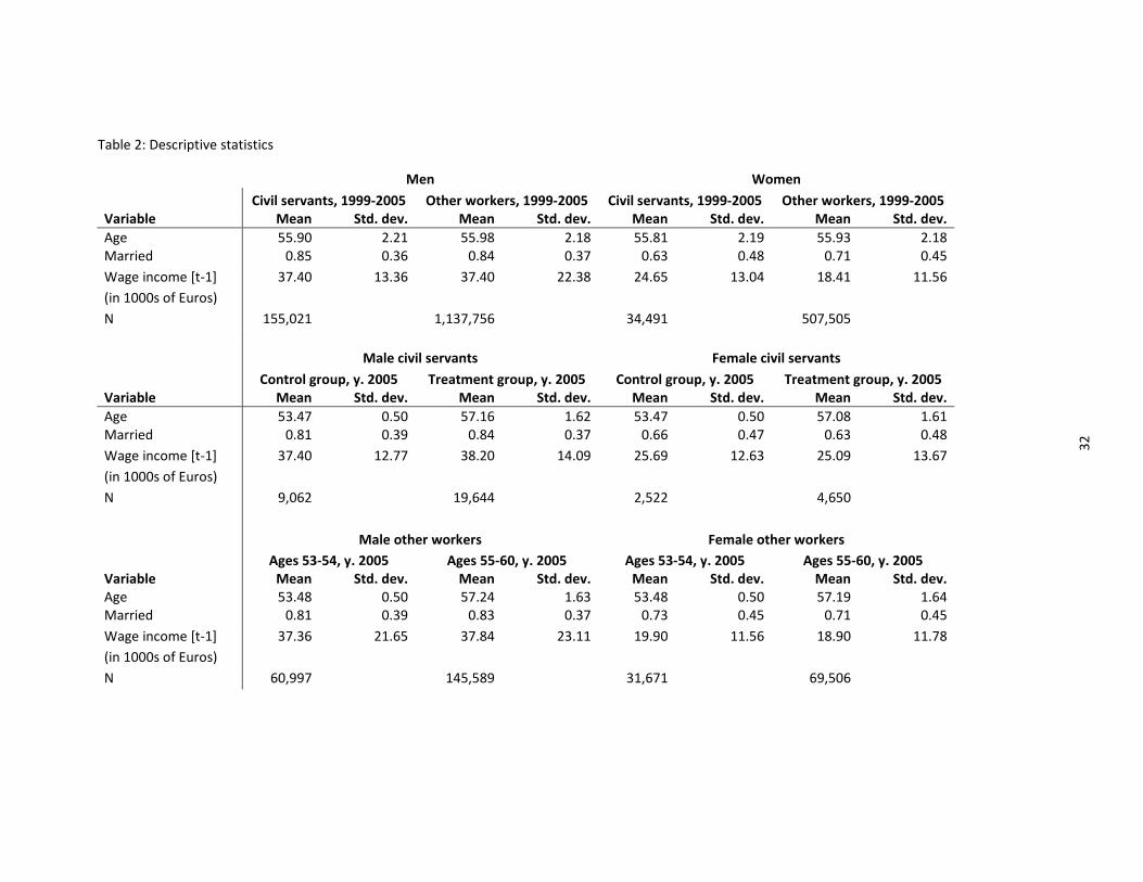
32
Table 2: Descriptive statistics
Men Women
Civil servants, 1999‐2005 Other workers, 1999‐2005 Civil servants, 1999‐2005 Other workers, 1999‐2005 Variable Mean Std. dev. Mean Std. dev. Mean Std. dev. Mean Std. dev.
Age 55.90 2.21 55.98 2.18 55.81 2.19 55.93 2.18Married 0.85 0.36 0.84 0.37 0.63 0.48 0.71 0.45
Wage income [t‐1]
(in 1000s of Euros)
37.40
13.36 37.40 22.38 24.65
13.04 18.41 11.56
N 155,021 1,137,756 34,491 507,505
Male civil servants Female civil servants
Control group, y. 2005 Treatment group, y. 2005 Control group, y. 2005 Treatment group, y. 2005 Variable Mean Std. dev. Mean Std. dev. Mean Std. dev. Mean Std. dev.
Age 53.47 0.50 57.16 1.62 53.47 0.50 57.08 1.61Married 0.81 0.39 0.84 0.37 0.66 0.47 0.63 0.48
Wage income [t‐1]
(in 1000s of Euros)
37.40
12.77 38.20 14.09 25.69
12.63 25.09 13.67
N 9,062 19,644 2,522 4,650
Male other workers Female other workers
Ages 53‐54, y. 2005 Ages 55‐60, y. 2005 Ages 53‐54, y. 2005 Ages 55‐60, y. 2005 Variable Mean Std. dev. Mean Std. dev. Mean Std. dev. Mean Std. dev.Age 53.48 0.50 57.24 1.63 53.48 0.50 57.19 1.64Married 0.81 0.39 0.83 0.37 0.73 0.45 0.71 0.45
Wage income [t‐1]
(in 1000s of Euros)
37.36
21.65 37.84 23.11 19.90
11.56 18.90 11.78
N 60,997 145,589 31,671 69,506

33
Table 3: Uninstrumented fixed effects estimates for the probability to die within five years for civil
servants*
Dif‐in‐dif Dif‐in‐dif‐in‐dif
Men Women Men Women
N 147,283 32,495 1,233,529 514,117
Coefficient estimate
retirement
P‐value
0.006
0.000
‐0.001
0.465
0.004
0.000
0.001
0.005
Fraction of total variation
explained by individual fixed
effects
0.802
0.796
0.802
0.803
Table 4: Fixed effects instrumental variable estimates for the probability to die within five years*
Dif‐in‐dif Dif‐in‐dif‐in‐dif
Men Women Men Women
N 147,283 32,495 1,233,529 514,117
Coefficient estimate retirement ‐0.025 ‐0.003 ‐0.025 ‐0.002
P‐value 0.058 0.889 0.057 0.889
F statistic on instruments in first stage 196.77 32.83 173.98 34.94
P‐value 0.000 0.000 0.000 0.000
P‐value J statistic 0.231 0.043 0.231 0.045
Fraction of total variation explained by individual fixed effects in first stage 0.301 0.349 0.470 0.662 Fraction of total variation explained by individual fixed effects in second stage 0.803 0.796 0.803 0.804
* The model estimated here controls for lagged wage income, marital status, year fixed effects,
nonlinear age effects and individual fixed effects. The p‐values on the coefficient are based on
heteroskedasticity robust standard errors.

34
Table 5: Fixed effects instrumental variable estimates for the probability to die within five years for male civil servants
(difference‐in‐difference)*
Cause of death LATE P‐value P‐value J statistic
LATE (in # of deaths)
# of deathsciv. serv., 1999‐2010
Neoplasms ‐0.003 0.761 0.002 ‐7.2 838 Malignant neoplasms of lip, oral cavity and pharynx ‐0.001 0.352 0.188 ‐2.6 20 Malignant neoplasms of digestive organs 0.002 0.709 0.095 5.4 266 Malignant neoplasms of respiratory and intrathoracic organs ‐0.002 0.654 0.379 ‐5.8 228 Melanoma and other malignant neoplasms of skin 0.001 0.609 0.231 2.0 34 Malignant neoplasms of mesothelial and soft tissue ‐0.000 0.780 0.367 ‐1.0 18 Malignant neoplasms of male genital organs ‐0.001 0.492 0.666 ‐3.3 49 Malignant neoplasms of urinary tract ‐0.002 0.550 0.079 ‐3.7 70 Malignant neoplasms of eye, brain and other parts of central nervous system ‐0.003 0.191 0.164 ‐6.1 43 Malignant neoplasms of ill‐defined, secondary and unspecified sites 0.001 0.600 0.082 2.7 34
Malignant neoplasms, stated or presumed to be primary, of lymphoid, haematopoietic and related tissue 0.002 0.527 0.290 4.4 61
Neoplasms of uncertain or unknown behavior 0.000 0.385 0.708 0.7 15Endocrine, nutritional and metabolic diseases ‐0.001 0.614 0.479 ‐1.5 22Mental and behavioural disorders ‐0.001 0.189 0.249 ‐1.9 15Diseases of the nervous system ‐0.001 0.580 0.830 ‐1.5 26Diseases of the circulatory system ‐0.007 0.311 0.996 ‐15.7 452 Hypertensive diseases ‐0.002 0.257 0.083 ‐3.6 22 Ischaemic heart diseases ‐0.006 0.170 0.888 ‐14.1 215 Other forms of heart disease 0.007 0.085 0.025 17.1 138 Cerebrovascular diseases ‐0.005 0.004 0.555 ‐11.9 51 Diseases of arteries, arterioles and capillaries ‐0.001 0.288 0.623 ‐3.2 28Diseases of the respiratory system 0.002 0.474 0.150 3.5 33Diseases of the digestive system ‐0.007 0.004 0.097 ‐17.0 49Symptoms, signs and abnormal clinical and laboratory findings, not elsewhere classified ‐0.004 0.220 0.982 ‐8.9 88External causes of morbidity and mortality ‐0.004 0.089 0.849 ‐9.1 69Other diseases ‐0.000 0.970 0.452 ‐0.2 28
Total ‐0.025 ‐59.4 1,621
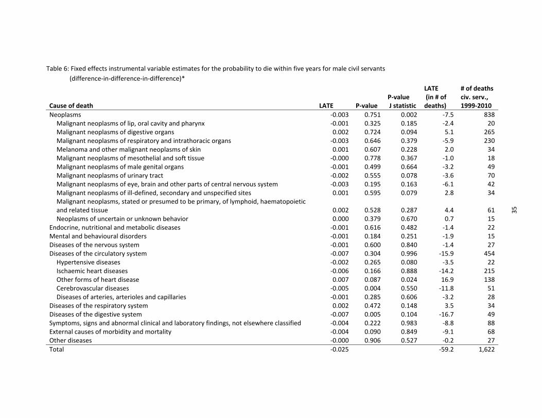
35
Table 6: Fixed effects instrumental variable estimates for the probability to die within five years for male civil servants
(difference‐in‐difference‐in‐difference)*
Cause of death LATE P‐value P‐value J statistic
LATE (in # of deaths)
# of deathsciv. serv., 1999‐2010
Neoplasms ‐0.003 0.751 0.002 ‐7.5 838 Malignant neoplasms of lip, oral cavity and pharynx ‐0.001 0.325 0.185 ‐2.4 20 Malignant neoplasms of digestive organs 0.002 0.724 0.094 5.1 265 Malignant neoplasms of respiratory and intrathoracic organs ‐0.003 0.646 0.379 ‐5.9 230 Melanoma and other malignant neoplasms of skin 0.001 0.607 0.228 2.0 34 Malignant neoplasms of mesothelial and soft tissue ‐0.000 0.778 0.367 ‐1.0 18 Malignant neoplasms of male genital organs ‐0.001 0.499 0.664 ‐3.2 49 Malignant neoplasms of urinary tract ‐0.002 0.555 0.078 ‐3.6 70 Malignant neoplasms of eye, brain and other parts of central nervous system ‐0.003 0.195 0.163 ‐6.1 42 Malignant neoplasms of ill‐defined, secondary and unspecified sites 0.001 0.595 0.079 2.8 34
Malignant neoplasms, stated or presumed to be primary, of lymphoid, haematopoietic and related tissue 0.002 0.528 0.287 4.4 61
Neoplasms of uncertain or unknown behavior 0.000 0.379 0.670 0.7 15Endocrine, nutritional and metabolic diseases ‐0.001 0.616 0.482 ‐1.4 22Mental and behavioural disorders ‐0.001 0.184 0.251 ‐1.9 15Diseases of the nervous system ‐0.001 0.600 0.840 ‐1.4 27Diseases of the circulatory system ‐0.007 0.304 0.996 ‐15.9 454 Hypertensive diseases ‐0.002 0.265 0.080 ‐3.5 22 Ischaemic heart diseases ‐0.006 0.166 0.888 ‐14.2 215 Other forms of heart disease 0.007 0.087 0.024 16.9 138 Cerebrovascular diseases ‐0.005 0.004 0.550 ‐11.8 51 Diseases of arteries, arterioles and capillaries ‐0.001 0.285 0.606 ‐3.2 28Diseases of the respiratory system 0.002 0.472 0.148 3.5 34Diseases of the digestive system ‐0.007 0.005 0.104 ‐16.7 49Symptoms, signs and abnormal clinical and laboratory findings, not elsewhere classified ‐0.004 0.222 0.983 ‐8.8 88External causes of morbidity and mortality ‐0.004 0.090 0.849 ‐9.1 68Other diseases ‐0.000 0.906 0.527 ‐0.2 27
Total ‐0.025 ‐59.2 1,622

36
Table 7: Fixed effects instrumental variable estimates for the probability to die within one to four years for male civil servants (difference‐in‐difference)*
Difference‐in‐difference Difference‐in‐difference‐in‐difference
The probability to die within 1 year 2 years 3 years 4 years 1 year 2 years 3 years 4 years
N 147,283 147,283 147,283 147,283 1,233,529 1,233,529 1,233,529 1,233,529 Coefficient estimate retirement
‐0.017 ‐0.022 ‐0.023 ‐0.028 ‐0.017 ‐0.022 ‐0.023 ‐0.029
P‐value 0.052 0.038 0.050 0.020 0.054 0.039 0.048 0.019 P‐value J statistic 0.553 0.182 0.702 0.388 0.545 0.179 0.702 0.386 Fraction of total variation explained by individual fixed effects in second stage
0.387 0.656 0.730 0.777 0.388 0.650 0.729 0.774
* The models estimated here controls for lagged wage income, marital status, year fixed effects, nonlinear age effects and individual fixed effects. The
p‐values on the coefficient are based on heteroskedasticity robust standard errors.

37
Table 8: Robustness checks on functional form*
LATE estimates for Dif‐in‐dif Dif‐in‐Dif‐in‐Dif
Variation LATE P‐value LATE P‐value
a. FE IV 2nd, 3rd order age effects ‐0.025 0.058 ‐0.025 0.057
b. FE IV 2nd order age effects ‐0.029 0.059 ‐0.029 0.059
c. FE IV 2nd, 3rd, 4th order age effects ‐0.025 0.067 ‐0.025 0.067
d. FE IV for married workers only ‐0.023 0.101 ‐0.023 0.100
e. FE IV incl. lagged wage income partner
and lagged retirement status partner
‐0.023 0.101 ‐0.019 0.110
f. FE IV for dataset incl. workers aged 52 ‐0.025 0.043 ‐0.026 0.042
g. FE IV for workers hospitalized before
retirement only
‐0.064 0.063 ‐0.064 0.064
h. FE IV for dataset incl. workers
hospitalized before retirement
‐0.029 0.024 ‐0.028 0.024
Table 9: Random effects instrumental variable estimates for the probability to die within five years*
LATE estimates for Dif‐in‐dif Dif‐in‐Dif‐in‐Dif
LATE P‐value LATE P‐value
RE IV ‐0.031 0.010 ‐0.031 0.013
Statistic P‐value Statistic P‐value
Hausman test 44.56 0.000 269.02 0.000
* The model estimated here controls for lagged wage income, marital status, year fixed effects,
nonlinear age effects and individual fixed effects. The p‐values are based on heteroskedasticity
robust standard errors.

38
Table 10: Hypothesized LATEs**
Probability to die within 1 year 2 years 3 years 4 years 5 years 6 years 7 years 8 years
(Hypothesized) coefficient retirement ‐0.017 ‐0.022 ‐0.023 ‐0.028 ‐0.025 ‐0.024 ‐0.019 0.000
** These hypothesized LATES are used to make a back‐of‐the‐envelope calculation on the amount of
pension benefits that are paid extra due to retired civil servants living longer than civil servants who
are not induced to retire by the introduction of the early retirement arrangement.