Embed Size (px)
Citation preview

THE CAPSTONE PROJECT OF ROALD E. PETERSON, JR. IS APPROVED.
DR. MARK M. BURROUGHS
DR. BRADLEY G. MAUGER
DR. TOM L. RIGGSCOMMITTEE CHAIRMAN
COLORADO TECH1992
COLORADO TECH
DESIGN OF A 408 MHz
HELICAL RADIO TELESCOPE
A CAPSTONE PROJECT SUBMITTED TO
DR. TOM L. RIGGS, JR.
IN CANDIDACY FOR THE DEGREE OF
MASTER OF SCIENCE
DEPARTMENT OF MATH, SCIENCE AND ENGINEERING
BY
ROALD E. PETERSON, JR.
COLORADO SPRINGS, COLORADO
SEPTEMBER 1992

HYPOTHESIS STATEMENT
A radio telescope capable of detecting useful thermal and non-thermal radiation from extraterrestrial
sources in the 408 MHz frequency range can be designed with an array of four helical beam antennas.

ABSTRACT
An intermediate amateur class radio telescope is designed, one subsystem at a time. The majority of
the design work centers on an array of four helical beam antennas which serve as the antenna subsystem. The
telescope's operating frequency is 408 Megahertz and it is able to detect extraterrestrial radio sources at or
below the level of 10 Janskys (1x1025 Watts/mVHz.) The design or selection of the other subsystems is also
covered. They include the transmission line, the receiver, the signal integrator, and the analog-to-digital
converter. The telescope is designed for a generic interface with any computer through the RS-232 serial port
for data recording and processing.
in
TABLE OF CONTENTS
THESIS STATEMENT ii
ABSTRACT iii
LIST OF ILLUSTRATIONS v
LIST OF TABLES vi
LIST OF APPENDICES vii
1. INTRODUCTION 1
2. SELECTION OF FREQUENCY RANGE 4
3. ANTENNA ARRAY DESIGN 6
4. TRANSMISSION LINE DESIGN 16
5. RECEIVER SELECTION 20
6. INTEGRATOR DESIGN 23
7. RECORDING SYSTEM SELECTION 26
8. CONCLUSION 28
APPENDICES 32
SELECTED BIBLIOGRAPHY 44
^
I V
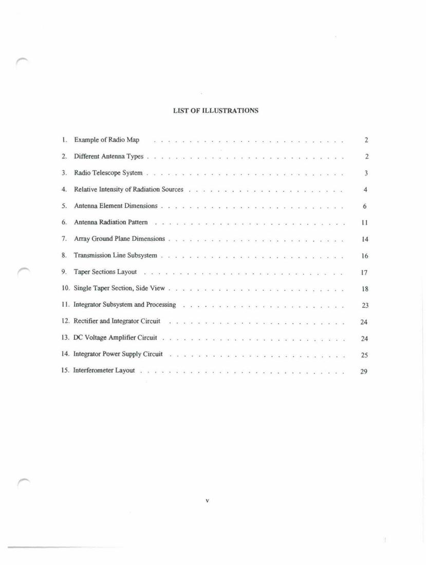
LIST OF ILLUSTRATIONS
1. Example of Radio Map 2
2. Different Antenna Types 2
3. Radio Telescope System 3
4. Relative Intensity of Radiation Sources 4
5. Antenna Element Dimensions 6
6. Antenna Radiation Pattern 11
7. Array Ground Plane Dimensions 14
8. Transmission Line Subsystem 16
9. Taper Sections Layout 17
10. Single Taper Section, Side View 18
11. Integrator Subsystem and Processing 23
12. Rectifier and Integrator Circuit 24
13. DC Voltage Amplifier Circuit 24
14. Integrator Power Supply Circuit . . . . 25
15. Interferometer Layout 29
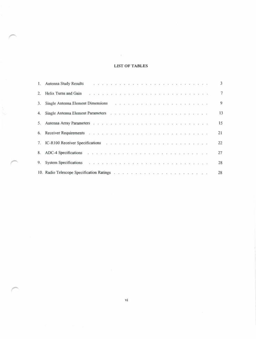
LIST OF TABLES
1. Antenna Study Results 3
2. Helix Turns and Gain 7
3. Single Antenna Element Dimensions 9
4. Single Antenna Element Parameters 13
5. Antenna Array Parameters 15
6. Receiver Requirements 21
7. IC-R100 Receiver Specifications 22
8. ADC-4 Specifications 27
9. System Specifications 28
10. Radio Telescope Specification Ratings 28
rvi

LIST OF APPENDICES
A. RADIO FREQUENCY BANDS 32
B. FREQUENCIES ALLOCATED TO RADIO ASTRONOMY 33
C. EXTRATERRESTRIAL RADIO SOURCES 34
D. HELICAL BEAM ANTENNA WORKSHEET 35
E. TAPER WIRE MATCHING SECTION WORKSHEET 38
F. RECEIVER SENSITIVITY WORKSHEET 39
G. RECEIVER DESCRIPTION 40
H. A/D CONVERTER DESCRIPTION 42
rvii
1. INTRODUCTION
This project presents the design of a radio telescope. Such a telescope consists • t a number of com-
ponents, each of which must be designed separately but with the other components in mind, to produce a
working system useful to the radio astronomer. This system is similar to larger research radio telescopes,
differing only in the antenna array size, component sophistication, and cost. In other words, the value of the
work which can be done with this telescope could be improved by increasing the size of the antenna array, or
purchasing more sensitive receiving equipment. This project is an outgrowth of my previous experience in
astronomy and a new interest in the radio portion of the electromagnetic spectrum. My intent was to gain a
much deeper understanding of both subjects by applying one to the other.
r^RADIO TELESCOPE SYSTEM DESCRIPTION
A radio telescope differs greatly from an optical telescope. An optical telescope may be small
enough to carry in one hand and provide the user with a magnified view of distant objects. In contrast, a ra-
dio telescope does not present the user with a ready made picture of the particular area of the universe he is
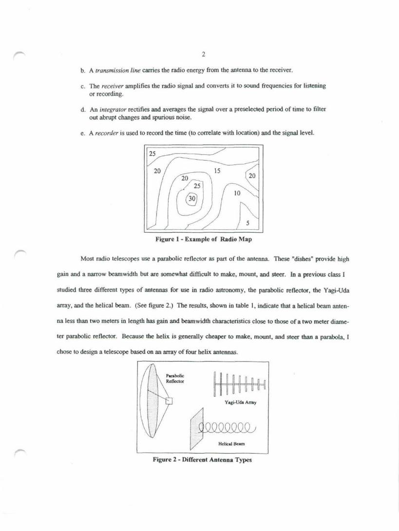
trying to observe. A radio telescope simply measures the intensity of noise in a particular area of sky and
records it. When intensities are recorded for several adjacent areas of the sky, they can be used to create
radio map of noise contours of the sky at a particular frequency. This concept is illustrated in figure 1.
The radio telescope consists of several subsystems which must work together to gather the data nec-
essary to produce a radio picture. While other components may be added to enhance the system, the follow-
ing list describes the minimum system required for a radio telescope. These components will be found in all
systems:
a. The antenna is used to capture and concentrate radio energy from a chosen portion of thesky.
a
1
b. A transmission line carries the radio energy from the antenna to the receiver.
c. The receiver amplifies the radio signal and converts it to sound frequencies for listeningor recording.
d. An integrator rectifies and averages the signal over a preselected period of time to filterout abrupt changes and spurious noise.
e. A recorder is used to record the time (to correlate with location) and the signal level.
Figure 1 - Example of Radio Map
Most radio telescopes use a parabolic reflector as part of the antenna. These "dishes" provide high
gain and a narrow beamwidth but are somewhat difficult to make, mount, and steer. In a previous class I
studied three different types of antennas for use in radio astronomy, the parabolic reflector, the Yagi-Uda
array, and the helical beam. (See figure 2.) The results, shown in table 1, indicate that a helical beam anten-
na less than two meters in length has gain and beamwidth characteristics close to those of a two meter diame-
ter parabolic reflector. Because the helix is generally cheaper to make, mount, and steer than a parabola, I
chose to design a telescope based on an array of four helix antennas.
Yagi-Uda Amy
Helical Beam
Figure 2 - Different Antenna Types

Antenna
Parabolic Reflector
Yagi-Uda Array (16 element)
Helical Beam (12 turn)
Gain
16.7dB
13.1 dB
15.3dB
Beam width
26.5 deg
26.0 deg
32.9 deg
Dimension
2.00m
1.62m
1.84m
Table 1 - Antenna Study Results
PROJECT OVERVIEW
This project includes the design or selection of all the components shown in figure 3. While the out-
line of a computer is shown, I have only presented the serial interface and not the computer itself, nor have
I designed storage or processing software. These elements are beyond the scope of this project.
Helical Radio Telescope System
Antenna Array TransmissionLine
Receiver Integrator A/DConverter
.'.'.'.'.'.>/.'.-:'.'.'.•'.ill!!
Computer
Figure 3 - Radio Telescope System
The next section will discuss the selection of a frequency range used in the design of the subsystems.
Following that, each subsystem design or selection will be discussed in detail, and in conclusion, the project
results will be summarized.

2. SELECTION OF FREQUENCY RANGE
There are numerous sources of radio energy in the universe. (See appendix C.) Some sources are
from nearby planets and Earth's sun. Others, such as quasars, are at the very edge of the visible universe,
about 15 billion light-years away. Radiation sources may be classified in two groups, thermal and nonther-
mal. These two groups are primarily active in different portions of the electromagnetic spectrum (see figure
4) but overlap in the UHF region. (Appendix A lists the radio frequency bands.) Nonthermal radiation results
primarily from plasma oscillation and synchrotron radiation and is most intense in the lower VHP region.
Thermal radiation is produced by any body above absolute zero and is roughly proportional to the tempera-
ture of the radiating body. Thermal radiation becomes noticeable in the VHP region and grows in intensity
through the X-ray region, where it then falls off rapidly (Heiserman 1977.)
r
VHP UHF n wave Visible X-rayFrequency
Figure 4 - Relative Intensity of Radiation Sources (Heiserman 1977)
I selected a telescope operating frequency in the UHF region for two reasons. First, I wanted to be
able to detect both thermal and nonthermal radio sources, and second, lower frequencies require larger anten-
nas because of the longer wavelength. Specific frequencies have been set aside by the various regulatory
4

5
agencies for use in different activities, including radio astronomy. After reviewing the frequencies allo-
cated to radio astronomy (see appendix B), I selected 406.1 MHz to 410.0 MHz as the target band for radio
observation. Having selected the target radio band, a frequency in the center of that region was chosen to be
the target frequency. To find the center frequency I used
fcenter =flaw + ̂ ^ = 408.05A///2
where flow is 406.1 MHz and f,,, is 410 MHz. Rounding off to 408 MHz is sufficient for this project. Next, the
wavelength was determined by dividing the speed of light by the frequency.
•s 3xl010cm/sec n-
With the target frequency and wavelength selected, the actual design process can begin.
r
3. ANTENNA ARRAY DESIGN
The antenna is an array of four helical beam antenna elements. The helical beam antenna was in-
vented by John Kraus in 1947 and is usually made from a single conductor wound in a spiral or helix (King &
Wong 1984.) In this application the helix functions in the axial mode as an end-fire array of circular anten-
nas with circular polarization. This gives the helix an advantage over some other types of antennas used for
radio astronomy because radiation coming from space is randomly polarized. Helical antennas respond to all
linearly polarized radiation equally. The design process consists of two parts, the design of a single antenna
element and the design of an array of four elements. Since the design is complex, with many design vari-
ables, I used Mathcad, a mathematical analysis tool, to help in the design. Mathcad allowed me to consider
several parametric inputs while eliminating the need to recalculate the equations by hand. I used the methods
found in the ARRL Antenna Book (1991) for all antenna design, except where noted.
SINGLE ELEMENT DESIGN
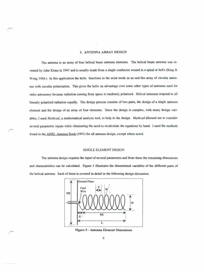
The antenna design requires the input of several parameters and from these the remaining dimensions
and characteristics can be calculated. Figure 5 illustrates the dimensional variables of the different parts of
the helical antenna. Each of these is covered in detail in the following design discussion.
Figure 5 - Antenna Element Dimensions
6

I selected several other input parameters as well as the frequency as a starting point for the antenna
design. 1 selected the number of turns, N, to be 12. This provides adequate gain and keeps the length of the
antenna below 2 meters. An appreciable increase in gain over that achieved with 12 turns would require sub-
stantially more turns. (See table 2. The calculation method is shown on page 10.) A total of 24 turns would
only result in a 3 dB improvement over a selection of 12 turns.
Turns
2.0
4.0
6.0
8.0
10.0
12.0
14.0
16.0
18.0
20.0
22.0
24.0
Gain (dB)
7.3
10.3
12.1
13.3
14.3
15.1
15.8
16.4
16.9
17.3
17.7
18.1
Table 2 - Helix Turns and Gain
Pitch is the angle, a, at which the helix wire winds forward along the antenna axis. The ARRL An-
tenna Book (1991) recommends a value for this from 12 to 16 degrees to provide maximum gain. I chose 12
degrees to keep the antenna as short as possible and stay within the recommended limits
The recommended helix circumference, C, is equal to the wavelength:
Also important in the design is the circumference given in wavelengths, Cx. This is found by dividing the cir-
cumference by the wavelength.
= f =1.0

8
The helix diameter, D, can be calculated from the circumference.
D = £ = .234 m
The space between loops, S, can be calculated from the wavelength and the pitch.
5=Xsina = .153 m
It is also useful to know this in terms of wavelength.
Sx = f = .208
The ARRL Antenna Book (1991) recommends the space between the back plane and the first turn,
G, be between . 12A. and . 13X. Again, I chose the smallest recommended value to minimize the antenna
length.
The antenna length, L, is calculated from the number of turns, the space between them, and the space
between the first rum and the back plane.
L = NS + G= 1.923 m
The ground plane diameter for a single helix, PD, should be between .8X and 1. IK {ARRL Antenna,
1991). Increasing the diameter increases the side lobes of the radiation pattern. Smaller diameters decrease
the gain. I chose the lowest recommended value to keep the antenna more manageable.
PD = .8 X = .588 m
This plane can be solid metal or, to keep it lighter and easier to work with, it can also be a steel mesh screen
with a maximum mesh spacing, MS, given by (Hyde 1963)
MS < . 125 X = . 092m
Metal window screen or chicken wire meets this requirement very nicely. However, a frame will have to be
built to support the screen. This can be 3/4" electrical conduit, cut and brazed to form a square.

The diameter of the helix conductor, HD, isn't a precise requirement but should be
.006 X < HD > .05 X
or between .44 and 3.68 cm. The upper limit is unreasonable. It's too hard to bend pipe into a spiral. The
lower limit requires a wire gauge of 5 or larger. This is too heavy when using solid copper or steel but alumi-
num or copper tubing can be used. However, I elected to use coaxial cable. It is light weight, bends extreme-
ly easily, and is low cost. Almost any coax will do. I only found one (RG-174) that was too small in
diameter for the .44 cm minimum requirement. The outer and inner conductors should be soldered together at
both ends to produce a "single" conductor. A wooden skeleton or cardboard tube is used as a permanent form
on which to wind the coaxial cable.
The final dimension of a single element is the linear length, LL, of cable required to produce the he-
lix. This can be found by
LL = ̂ - = 8.84 m
A summary of the single element antenna dimensions are given below in table 3.
Dimension
Number of turns
Pitch angle
Circumference
Diameter
Circumference in X
Space between turns
Turn space in A.
Distance to ground plane
Length of antenna
Ground plane diameter
Max. plane mesh size
Min. helix conductor diam.
Linear length of conductor
Symbol
N
u
C
D
cxsSx
G
L
PD
MS
HD
LL
Value
12
12
0.735
0.234
1
0.153
0.208
0.088
1.924
0.588
7.4
0.44
8.83
Units
turns
deg
m
m
X
m
X
m
m
m
cm
cm
m
Table 3 - Single Antenna Element Dimensions
10
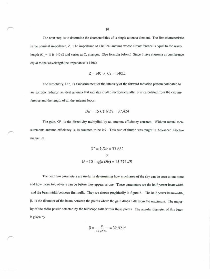
The next step is to determine the characteristics of a single antenna element. The first characteristic
is the nominal impedance, Z. The impedance of a helical antenna whose circumference is equal to the wave-
length (Cx = 1) is 140 Q and varies as Cx changes. (See formula below.) Since I have chosen a circumference
equal to the wavelength the impedance is 140Q.
Z=140 x Cx
magnetics.
The directivity, Dir, is a measurement of the intensity of the forward radiation pattern compared to
an isotropic radiator, an ideal antenna that radiates in all directions equally. It is calculated from the circum-
ference and the length of all the antenna loops.
Dir = 15 ClN ̂ = 37.424
The gain, G*, is the directivity multiplied by an antenna efficiency constant. Without actual mea-
surements antenna efficiency, k, is assumed to be 0.9. This rule of thumb was taught in Advanced Electro-
G* = k Dir = 33.682
or
G= 10 \Qg(kDir)= \5.274dB
The next two parameters are useful in determining how much area of the sky can be seen at one time
and how close two objects can be before they appear as one. These parameters are the half power beamwidth
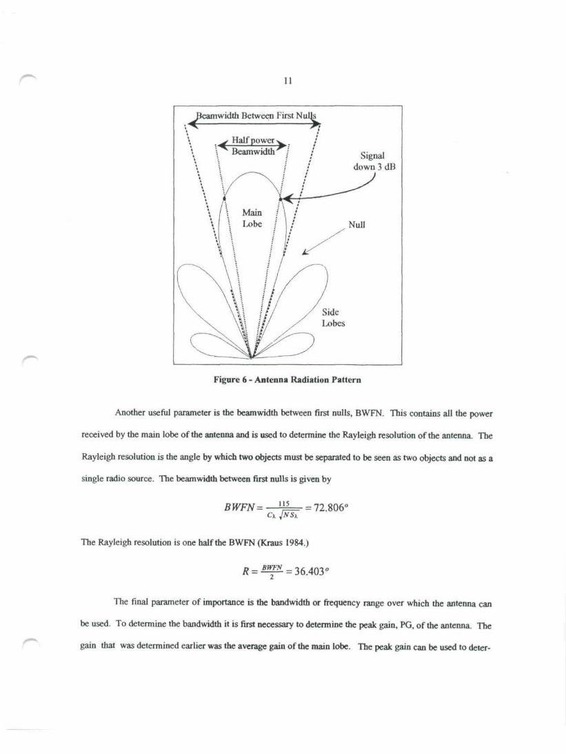
and the beamwidth between first nulls. They are shown graphically in figure 6. The half power beamwidth,
|3, is the diameter of the beam between the points where the gain drops 3 dB from the maximum. The major-
ity of the radio power detected by the telescope falls within these points. The angular diameter of this beam
is given by
= 32.921°
^
Beamwidth Between First Nulls
Half power <Beamwidth Signal
down 3 dB
SideLobes
Figure 6 - Antenna Radiation Pattern
Another useful parameter is the beamwidth between first nulls, BWFN. This contains all the power
received by the main lobe of the antenna and is used to determine the Rayleigh resolution of the antenna. The
Rayleigh resolution is the angle by which two objects must be separated to be seen as two objects and not as a
single radio source. The beamwidth between first nulls is given by
BWFN= — T==^ = 72.806°
The Rayleigh resolution is one half the BWFN (Kraus 1984.)
= 36.403"
The final parameter of importance is the bandwidth or frequency range over which the antenna can
be used. To determine the bandwidth it is first necessary to determine the peak gain, PG, of the antenna. The
gain that was determined earlier was the average gain of the main lobe. The peak gain can be used to deter-

12
mine the bandwidth frequency ratio, BFR, which is the ratio of the nigh frequency limit to the low frequency
limit. This method for determining bandwidth was presented by King and Wong (1984) and provides the an-
tenna bandwidth at which the antenna gain is 2 dB down.
I"PG = 8.3 (^£.)7»*a-« (Msx).8 (iHLi^l)— = 18 552 dB
The bandwidth frequency ratio is determined by
lw =1.112
This ratio can be used to determine the half bandwidth, Af, above and below the nominal frequency.
The total bandwidth (2 dB down) of the antenna then is twice the frequency computed above.
This provides several times the bandwidth needed to cover the 406 - 410 MHz frequency allotted to radio as-
tronomy in this region of the spectrum. The actual high and low frequency limits are
Fw=/+4f= 429.6 Mfe
Fh=f-Af= 386.4 MHz
This completes the calculation of the necessary parameters. They are summarized in table 4.

13
Parameter
Impedance
Directivity
Gain (algebraic)
Gain
Half Power Beamwidth
Beamwidth - first nulls
Resolution
Bandwidth (2 dB down)
High frequency limit
Low frequency limit
Symbol
Z
Dir
G*
G
PBWFN
R
BW
f*
f,o
Value
140
37.42
33.68
15.27
32.92
72.81
36.4
43.29
429.6
386.4
Units
Q
dB
deg
deg
degMHz
MHz
MHz
Table 4 - Single Antenna Element Parameters
ARRAY DESIGN
The design of the individual antenna element and determining its parameters are the most time con-
suming and involved parts of the entire project. While a single helix would suffice for good quality entry lev-
el radio astronomy explorations, an array of four antennas greatly increases the gain and resolution. Fainter
radio sources can be detected and smaller objects or portions of the sky can be discerned. More precise work
could be done with a larger array to increase sensitivity or an interferometer of several arrays, spaced
several wavelengths apart to improve resolution. This array is built with four of the helical elements designed
previously. The methods used in the array design process are also taken from the ARRL Antenna Rppk
(1991) unless otherwise noted.
The four helices are attached to a ground plane made of conduit and screen as mentioned earlier.
This ground plane will in turn be attached to an altazimuth mount to allow the telescope antenna to be di-
rected toward any desirable spot in the sky. The dimensions for placement of the helices on the ground plane
will be calculated next. Placement is simple and determined solely from the wavelength of the operating fre-
quency (see figure 7.) Again, increasing the size of the reflector will increase the size of the side lobes and
decreasing the reflector size will decrease the forward gain.
"~

14
.5 A.
Figure 7 - Array Ground Plane Dimensions
The length of the sides, LS, of the ground plane is
£5 = 2.5 X= 1.838ro
The distance, DE, from each antenna element to the edge of the ground plane is
The distance, DH, between helices along the edge of the ground plane, not diagonally, is
DH= 1.5 \= 1.103m
Next, the parameters of the array are determined. The simplest is the gain, GA*, which is found by
multiplying the gain of an individual element by the number of elements.
G'A=NExG* = 134.727
or
The array half power beamwidth, p A, is found to be
Px= /^p =17.498'A
The helix antenna acts like a radio lens, focusing energy onto itself from a greater area than its actual

15
physical cross section. In other words, the effective aperture is greater than the physical aperture. To deter-
mine the resolution I calculated the effective area of the array, EA, and from that the effective diameter of the
array, ED, and from that the resolution, RA. The effective area is
EA = = 5.797m2
This area has an effective diameter of
= 2 = 2.7llm
The resolution is then determined for an antenna with the effective diameter.
The array parameters are summarized in table 6. The antenna has substantially improved gain and
resolution over a single element. Additionally, the antenna is less than two meters long on any primary axis.
This will allow the telescope to be easily steered and will greatly reduce its sensitivity to wind. The next
step in the design process is to connect the antenna to the receiver. This is done via a transmission line.
Parameter Symbol
Array gain GA
Half power beamwidth (3A
Effective area EA
Effective diameter ED
Array resolution RA
Value
21.295
17.498
5.797
2.717
15.428
Units
dB
deg
m2
m
deg
Table 5 - Antenna Array Parameters

4. TRANSMISSION LINE DESIGN
! he transmission line is the subsystem of the radio telescope which carries the radio energy captured
by the antenna to the receiver. It is also a system of several components as shown in figure 8 below. The de-
sign methods for this portion of the telescope were taken from the ARRL Antenna Handbook (1991.)
AntennaElements Matching
Tapertions
50Coaxial
* Feed Line „50 n
200ft
Receiver50 Q
Figure 8 - Transmission Line Subsystem
The primary feed line leading to the radio receiver should be of the same impedance as the nominal
impedance of the receiver, 50 Q. According to the ARRL Electronics Data Book (DeMaw 1988) there are
several types of coaxial cable that can be used for this; RG-9B, RG-55A, RG-141, RG-142, RG-174, etc. I
chose RG-141 because of its smaller diameter, 0.190 in. This will make it easier to handle. The capacitance
per foot, 29.4 pF, is about the same as the others and its velocity factor, VF, is 70% with PTFE dielectric. Its
nominal impedance is 50 Q.
On the other end of the transmission line are four helical antennas, each with a characteristic im-
pedance of 140 Q. Since there are four antennas feeding into one line the antennas act as four resistors in
16

17
parallel feeding one point. At this point they must match the impedance of the feed line, 50 Q. If the anten-
nas are connected directly to the feed line they would have a combined impedance of
y _ 2ml _ _ I40_ _ TC r\Z"otal - Ant - -•>->"
Accordingly, there must be a matching section between the antennas and the feed line as shown in figure 7.
The impedance at the antenna of these matching sections should be the same as the impedance of the anten-
nas, 140 Q. The impedance at the other end can be found by multiplying the impedance of the line by the
number of antenna feeds.
Z,ine xAnt = 50x4 = 200 Q
Four of these sections in parallel will combine to produce 50 Q, matching the impedance of the feed line.
The simplest matching transformer I could find for this application is a taper section. These sections
connect the antennas to the center of the ground plane (see figure 9) where they are soldered to an appropriate
coax connector and the feed line can be connected to this junction point.
Ground Plane
Junction
Taper Section
Figure 9 - Taper Sections Layout
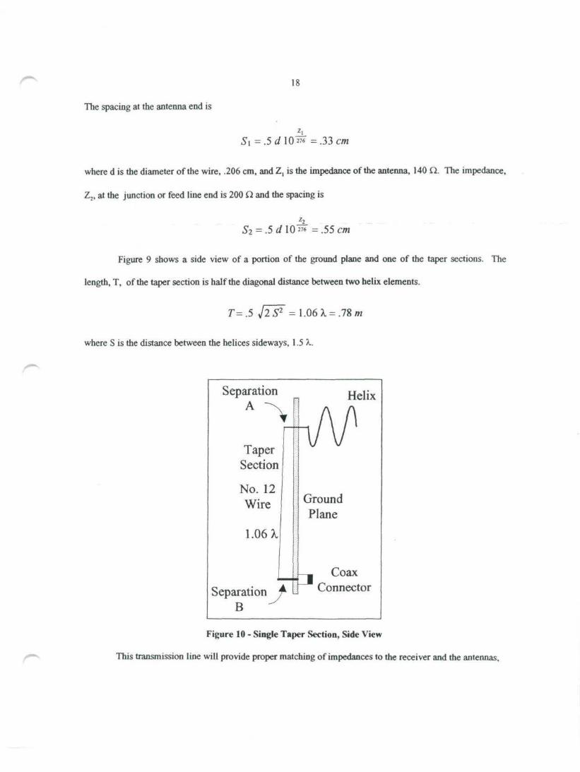
The taper sections are on the underside of the ground plane as shown in figure 10. They are con-
structed of 12 gauge copper wire and are separated from the ground plane by different distances at each end.
18
The spacing at the antenna end is
Si = . 5 < / 1 0 » « =.33 cm
where d is the diameter of the wire, .206 cm, and Z, is the impedance of the antenna, 140 Q. The impedance,
Z2, at the junction or feed line end is 200 Q and the spacing is
z2
S2 = .5d\Q™ =.55 cm
Figure 9 shows a side view of a portion of the ground plane and one of the taper sections. The
length, T, of the taper section is half the diagonal distance between two helix elements.
r=.5 v/25"2 = 1.06 X = .78m
where S is the distance between the helices sideways, 1.5 >..
Separation
TaperSection
No. 12Wire
1.06 A.
Separation 4B
Helix
CoaxConnector
Figure 10 - Single Taper Section, Side View
This transmission line will provide proper matching of impedances to the receiver and the antennas.

19
eliminating most standing wave ratio (SWR) losses in this portion of the system.
Instead of leading to the receiver, the transmission line could be connected to a low noise preamplifi-
er. However, as will be shown in the next section, this is not necessary for the telescope to function properly.
A preamplifier would increase the sensitivity of the instrument but is not critical to beginning and intermedi-
ate level observations.

5. RECEIVER SELECTION
A simple radio receiver could be built without an undue amount of trouble. The signal being de-
tected is noise and there is not much signal processing involved. One could build a wide band receiver for
very little cost, especially with the semiconductors available on today's market (Sickels, The Radio Astrono-
my Circuit Cookbook 1992.) However, there are receivers already designed in Sickels' books and, even bet-
ter, there are numerous receivers which can be purchased off the shelf which will satisfy radio astronomy
requirements and serve as general purpose receivers for other uses also. The primary purpose of this section
is to determine which receiver will function adequately for the telescope. Unless specified otherwise the
methods used in this selection process were presented by Heiserman (1977.)
The most important parameter to determine at this time is the receiver sensitivity required to detect
useful signals. To do this the lower limit for signal strength must be known. Robert Sickels has compiled a
list of 400 celestial radio sources with flux above 10 janskys (The Radio Astronomy Handbook. 1992.) A
jansky is a unit of radio power falling upon a square meter of the Earth's surface, per hertz and is named after
Karl Jansky who discovered radio emissions from the center of the Milky Way (Shields 1986)
I selected 10 janskys as the limit of minimum observable power flux. The next step is to find how
much power is available at the antenna. To do this the effective aperture of the antenna in square meters must
be known. This was previously determined to be 5.797 m2. (See table 5.) The other parameter needed is the
bandwidth of the receiver. Since a receiver hasnt yet been selected a parameter which is common to several
off the shelf receivers should be used. Most receivers have a wide FM bandwidth of 150 - 180 kHz. I chose
the lower end (150 kHz) simply because it is the most common wide band FM bandwidth. The power avail-
able at the antenna terminals, PA, is
20

21
PA=SAeB = 8.696 x JO'20 watts
S is the flux in watts/mVHz (10 janskys = 1x10 25 watts/mVHz), Ac is the effective area, and B is the band-
width in hertz. An alternate method to determine antenna power uses the antenna gain instead of the effective
area and comes extremely close, validating the first method.
G4
PA =7.17 x 10~^~ xBxS* 1(T23 x -jj- = 8.705 x 10"20 watts
The variable f is the operating frequency of the antenna in MHz, 408.
Receiver sensitivity is usually given as the number of microvolts at the input which produces an out-
put 10 dB above the internally generated noise. Radio astronomy has much less stringent receiver noise re-
quirements than music or voice radio. In fact, a recording system based on analog-to-digital conversion and
computer storage can easily discern signal levels 1% above the receiver noise floor or a signal-to-noise ratio
of .01. The power received by the antenna, 8.696 x 10²⁰ watts, the antenna impedance, 140 £1, and the
signal-to-noise ratio of .01 can be used to determine the required receiver sensitivity, SR.
9.091x!06 JP<ZA
This value doesn't take into account any losses. If we assume insertion and attenuation losses in the
transmission line of 3 dB, probably a worst case, we will come up with a more realistic sensitivity require-
ment. This cuts the power from the antenna in half, making the sensitivity requirement one half of that calcu-
lated above, or 1.586 nV.
The final step of receiver selection is finding a receiver which meets or exceeds the specifications
determined above. These specifications are summarized in table 6.
Specification
Bandwidth
Receiver sensitivity
Frequency range
Symbol
B
skF
Value
150
1.59
406-410
Units
kHz
nvMHz
Table 6 - Receiver Requirements

22
I sent for literature on several multiband and UHF receivers. After looking through the specifica-
tions, I found several which met the requirements but I chose the Icom IC-R100 multiband receiver over the
others for the following reasons:
1. It has very good sensitivity.
2. It has an extremely wide frequency range
3. It's capable of running on battery power.
4. Its very portable, weighing only 3 Ibs..
5. It's a relatively inexpensive multiband receiver (about S600.)
It can also be used as a receiver for radio telescopes in other frequency bands as well as general purpose radio
scanning and receiving. Selected specifications for the R100 are shown below. The complete specifications
are shown in Appendix G.
Specification
Bandwidth
Receiver sensitivity
Frequency range
Symbol
B
SR
F
Value
180kHz
0.63 nV
.5 -1800 MHz
Table 7 - IC-R100 Receiver Specifications
6. INTEGRATOR DESIGN
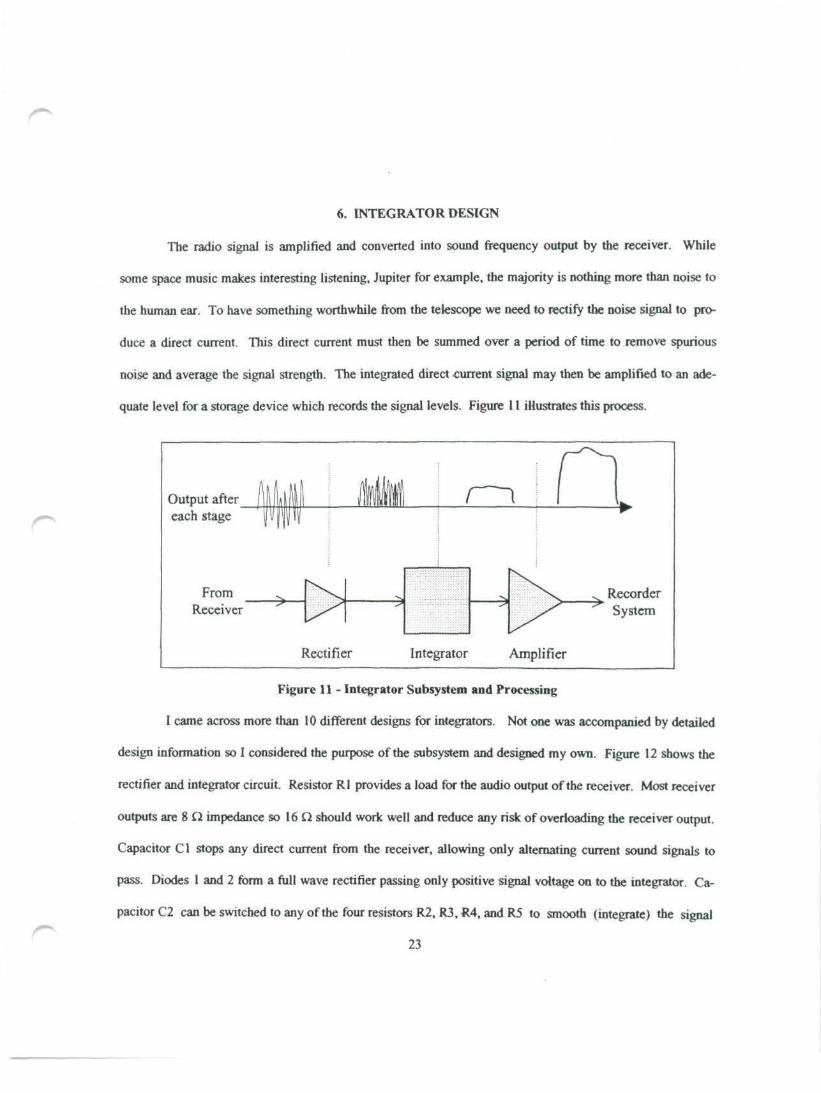
The radio signal is amplified and converted into sound frequency output by the receiver. While
some space music makes interesting listening, Jupiter for example, the majority is nothing more than noise to
the human ear. To have something worthwhile from the telescope we need to rectify the noise signal to pro-
duce a direct current. This direct current must then be summed over a period of time to remove spurious
noise and average the signal strength. The integrated direct current signal may then be amplified to an ade-
quate level for a storage device which records the signal levels. Figure 11 illustrates this process.
Output aftereach stage
FromReceiver
RecorderSystem
Rectifier Integrator Amplifier
Figure 11 - Integrator Subsystem and Processing
I came across more than 10 different designs for integrators. Not one was accompanied by detailed
design information so I considered the purpose of the subsystem and designed my own. Figure 12 shows the
rectifier and integrator circuit. Resistor Rl provides a load for the audio output of the receiver. Most receiver
outputs are 8 Q impedance so 16 Q should work well and reduce any risk of overloading the receiver output.
Capacitor Cl stops any direct current from the receiver, allowing only alternating current sound signals to
pass. Diodes 1 and 2 form a full wave rectifier passing only positive signal voltage on to the integrator. Ca-
pacitor C2 can be switched to any of the four resistors R2, R3, R4, and R5 to smooth (integrate) the signal
23

24
from the rectifier portion of the circuit. They have time constants of C2 x R, or about .5 second, 1 second, 5
seconds, and 10 seconds. This is variable to enable the telescope to detect different types of objects. Re-
sistor R6 discharges C2 when the signal drops.
Dl1N34
+ i i r^v.^ 1 1 1 - >J ^x
iRl <16 <
cni>
D2 71N34 "
±L aTio^r
? '
^
>R6> I Meg
/SSi
R2 R3 R4 R550K 100K 500K 1 Meg
Figure 12 - The Rectifier and Integrator Circuit
The direct current amplifier circuit is shown in figure 13. It is a simple non-inverting amplifier
based on an LM 741 or equivalent operational amplifier. Gain is controlled by potentiometer R3 and varies
from 1 to 101. This is used to keep the amplifier from being driven to saturation. Another potentiometer, R4,
allows the output voltage to be attenuated to avoid saturating the recording subsystem.
+12V
FromIntegrator
-9
Figure 13 - DC Voltage Amplifier Circuit
25
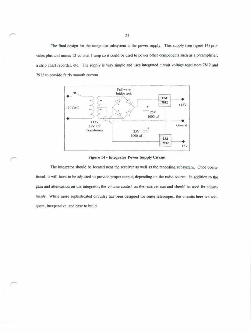
The final design for the integrator subsystem is the power supply. This supply (see figure 14) pro-
vides plus and minus 12 volts at 1 amp so it could be used to power other components such as a preamplifier,
a strip chart recorder, etc. The supply is very simple and uses integrated circuit voltage regulators 7812 and
7912 to provide fairly smooth current
Full wavebridge rect.
110VAC+ 12V
117V25V CT
Transformer
Ground
12V
Figure 14 - Integrator Power Supply Circuit
The integrator should be located near the receiver as well as the recording subsystem. Once opera-
tional, it will have to be adjusted to provide proper output, depending on the radio source. In addition to the
gain and attenuation on the integrator, the volume control on the receiver can and should be used for adjust-
ments. While more sophisticated circuitry has been designed for some telescopes, the circuits here are ade-
quate, inexpensive, and easy to build.

7. RECORDING SYSTEM SELECTION
The final subsystem records the output of the radio telescope. We can't see a nice picture of the uni-
verse directly so the data will have to be processed. The easiest way to record and process large amounts of
signal intensity data is with a computer. The processing methods are beyond the scope of this project. Nei-
ther will I specify particular computer hardware other than a computer with a serial port.
The only thing left to select is an analog-to-digital converter (ADC) to change the analog voltage
levels coming from the integrator to digital data and send it to a computer. I examined data acquisition litera-
ture from several vendors looking for the best system to meet my needs. My requirements were:
1. The system must have an RS-232 serial port to interface with an appropriate computer.
2. The ADC should be as low cost as possible.f^
3. The ADC must have a resolution of at least 1024 (10 bits) or .005 volts.
4. The ADC must cover a range of 0 to 5 volts and not more than 15 volts.
5. The ADC should have its own power supply or be capable of using the integrator supply.
6. The software to access the data must be simple and modifiable.
There were many ADC systems but most of them cost over $500 and used special cards to plug into
an IBM compatible (ISA) bus. The secret, it seems, is to stay away from the glossy catalogs and look in
small column advertisements. The ADC-4 from Electronic Energy Control, Inc. met or exceeded the above
requirements. Its specifications of interest are summarized in table 8 and the specification sheets are shown
in appendix H. The resolution is substantially better than the requirement and the voltage range is the same
as the requirement. Higher or lower voltage levels can be attenuated or amplified by the amplifier section of
the integrator. The ADC-4 has 4 channels which will allow for future expansion to a 4 antenna interferometer
telescope. The unit can also be powered from the integrator supply. An example of the software required to
access the data is shown in appendix H. It is simple and completely modifiable. The ADC-4 will also connect
26

27
to any computer with a serial port, and even allows the use of a modem for unattended observation. One
could leave the telescope in receive mode during vacation time and access the data with a computer over long
distance phone lines.
Specification
Resolution (increments)
Input range
Channels
RS-232 Baud rate
Power supply
Cost
Value
4096 (12 bit), <.002 V
0-5 V
4
50 - 19,200 baud
9- 14V, 300mA
$170
Table 8 - ADC-4 Specifications

8. CONCLUSION
This capstone project demonstrates that a radio telescope capable of detecting useful thermal and
non-thermal radiation from extraterrestrial sources in the 408 MHz frequency range can be designed around
an array of four helical beam antennas. The specifications of the instrument are summarized below in table 9.
Specification Value
Operating Frequency
Detection
Receiver Bandwidth
Antenna Bandwidth
Antenna Dimensions
Antenna Gain
Effective Diameter
Resolution
Sensitivity
Minimum Detectable Signal
A/D Convenor Resolution
Cost (excluding computer)
408MHz
Wideband FM
180kHz
43.3MHz
1.9 x 1.8x 1.8m
21.3 dB
2.7m
15.43 deg
.63 uV
< 10 Janskys
12 bits (.002V)
<S1000
Table 9 - System Specifications
If these specifications are compared to Heiserman's (1975) radio telescope parameter classifications (see Ta-
ble 10) their suitability to serious amateur work becomes apparent.
Parameter
Antenna Gain
Receiver Sensitivity
Receiver Bandwidth
Minimum
10 dB
5uV
100 kHz
Normal
15 dB
1 nV
2MHz
Excellent
20 dB
.5nV
6MHz
Table 10 - Radio Telescope Specification Ratings
The antenna gain is excellent while the receiver sensitivity is close to the excellent category. Gener-
ally, more sensitivity is required to detect usable radio noise. However, this system comes out extremely well
28
because it can detect signals below 10 janskys. Amateur instruments are usually capable of detecting no less
than 25 to 50 janskys (Sickels, Radio Astronomy Handbook. 1992.) Because the antenna gain is so high the
receiver sensitivity can be lower and still yield excellent detection ability. Originally, 1 expected a preampli-
fier would be needed to detect anything in the 10 jansky rant This project has shown it isn't necessary. The
use of a low noise preamplifier could easily lower the detection threshold below 1 jansky.
The receiver bandwidth is within the minimum range but well below the "normal." Wide bandwidth
is generally required to gather enough radio flux to be detected by the system. Since the telescope's detection
capabilities have been shown to be excellent, greater bandwidth is unnecessary. In fact, the system provides
greater frequency resolution than most amateur instruments and because the antenna bandwidth is extremely
wide the telescope can be used to observe the sky at several different frequencies.
The telescope operating frequency falls hi that area of the spectrum where thermal and non-thermal
radio noise levels are approximately equal (see figure 4.) This allows the different sources of these two types
of radiation to be observed with a single instrument. Further observations could be made at higher or lower
frequencies by using the antenna arrays wide bandwidth and changing the receiver operating frequency. The
antenna's operating frequency could even be changed by placing the antenna end of the taper sections on ny-
lon screws and adjusting the distance and impedance of the sections.
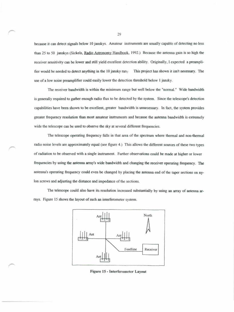
The telescope could also have its resolution increased substantially by using an array of antenna ar-
rays. Figure 15 shows the layout of such an interferometer system.
Ant North
Ant
Ant
Ant
Feedlinc
Figure 15 - Interferometer Layout

+1f.1'¥.
30
The antennas in such a system would be separated by several wavelengths of distance and would be
lined up on a north-south-east-west grid to provide increased resolution in both dimensions. The resolution of
such a system is given by
n _ 57 XK D
where R is the resolution in degrees, A, is the operating wavelength, and D is the distance between antennas in
wavelengths.
The receiver and ADC in the recording subsystem were off-the-shelf items but could be home built if
time were available. Several designs can be found in the books referenced in the bibliography, especially
Sickels'.
This design shows that a very usable radio telescope can be built with helical beam antennas. When
the gain, ease of construction, size, and mounting of such an instrument are compared to a parabolic dish an-
tenna it shows that the helix is an effective, if not better, alternative antenna design.
Robert Sickels is sort of a world wide coordinator of amateur radio astronomy. I found his phone
number in an astronomy magazine and talked with him about this project. It seems that there are very few
how-to books on the subject and almost none in print. The reason for this is that there are only about 700
amateur radio astronomers in the world. Sickels has several books available, numerous electronic supplies,
and publishes a monthly amateur astronomer's magazine called The Radio Observer. I have included his
company name and address for those readers who might wish to become more involved with this subject.
Bob's Electronic Service7605 Deland Ave.
Fort Pierce, Florida 34951Telephone: (407)464-2118
This project provided an excellent opportunity to learn about designing antenna systems and trans-
mission lines. It also provided a deeper look at radio astronomy, amateur radio, and the electromagnetic
spectrum. The systems design process was similar to the communications and computer systems designs I

31
have been involved with at work. I plan to build a radio telescope and also become more involved in ama-
teur radio. Overall, I enjoyed the project and feel it taught me a great deal.
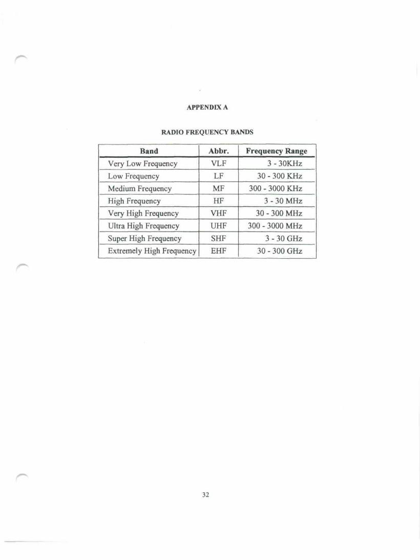
APPENDIX A
RADIO FREQUENCY BANDS
Band
Very Low Frequency
Low Frequency
Medium Frequency
High Frequency
Very High Frequency
Ultra High Frequency
Super High Frequency
Extremely High Frequency
Abbr.
VLF
LF
MF
HF
VHP
UHF
SHF
EHF
Frequency Range
3 - 30KHz
30 - 300 KHz
300 - 3000 KHz
3 - 30 MHz
30 - 300 MHz
300 - 3000 MHz
3 - 30 GHz
30 - 300 GHz
32

APPENDIX B
FREQUENCIES ALLOCATED 10 RADIO ASTRONOMY
Authority
FCC
FCC
World
FCC
FCC
FCC
FCC
FCC
FCC
FCC
World, FCC
FCC
FCC
FCC
FCC
FCC
FCC
FCC
FCC
FCC
FCC
FCC
FCC
FCC
Frequency
13.36- 13.41 MHz
25.55 - 25.67 MHz
37.50 - 38.25 MHz
73.0 - 74.6 MHz
406. 1-410.0 MHz
608 - 614 MHz
1400 - 1427 MHz
1660- 1670MHz
2665 - 2700 MHz
4990 - 5000 MHz
10.60 - 10.70 GHz
15.35- 15.40 GHz
22.21 -22.50 GHz
23.6 - 24.0 GHz
31.3-31. 8 GHz
42.5 - 43.5 GHz
58.2 - 59.0 GHz
72.72 - 72.91 GHz
86 - 92 GHz
105- 116 GHz
164- 168 GHz
182- 185 GHz
217 -231 GHz
265 - 275 GHz
Bandwidth
50 KHz
120 KHz
750 KHz
1.6MHz
3.9 MHz
6 MHz
27 MHz
10 MHz
35 MHz
10 MHz
100 MHz
50 MHz
290 MHz
400 MHz
500 MHz
1 GHz
800 MHz
190MHz
6 GHz
11 GHz
4 GHz
3 GHz
14 GHz
10 GHz
Comments
Shared
Shared
Shared
Center X
22.04 m
11.71 m
7.92m
4.07m
73.5 cm
49.1 cm
21.2cm
18.0cm
11.2cm
6.0 cm
2.82 cm
1.95cm
1.34 cm
1.26cm
9.51 mm
6.98 mm
5.12 mm
4.12mm
3.37 mm
2.71 mm
1.81 mm
1.63 mm
1.34 mm
1.11 mmTaken from the Federal Communications Commission's Table of Frequency Allocations (1991)

APPENDIX C
EXTRA-TERRESTRIAL RADIO SOURCES
Source Type Frequency Description
Jupiter-Io
Solar Flares
Sun
Meteors
Meteors
Quasars & RadioGalaxies
Milky Way
"Hot" Objects(Stars, Galaxies)
Planets
Hydrogen Line
Discrete
Discrete
Extended
Indirect
Indirect
Discrete
Discrete
Extended
Discrete
Extended
20 - 24 MHz
80 - 500 MHz
50 MHz - 3 GHz
80- 150 MHz
VHP
VHP - UHF
VHF-UHF
SHF +
EHF
1.428 GHz
Surf-like sound
Short bursts
Temperature radiation coming fromdifferent layers
Bounce signals off trails like radar
Listen to bounced VHP from overthe horizon transmitters
Very powerful, non-thermal signals
Synchrotron radiation
Thermal signals, with frequencydepending on temperature
Extremely low power thermalsignals
Neutral hydrogen spectral line
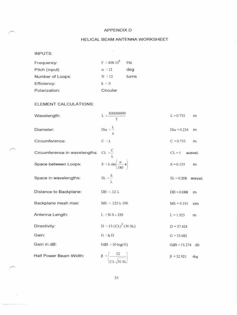
APPENDIX D
HELICAL BEAM ANTENNA WORKSHEET
INPUTS:
Frequency:
Pitch (input)
Number of Loops:
Efficiency:
Polarization:
ELEMENT CALCULATIONS:
Wavelength:
Diameter:
Circumference:
F. = 408-10° Hz
a =12 deg
N =12 turns
k . = .9
Circular
X:=300000000
Dia:=-JC
C -X
Circumference in wavelengths: CX = —X
Space between Loops:
Space in wavelengths:
Distance to Backplane:
Backplane mesh max:
Antenna Length:
Directivity:
Gain:
Gain in dB:
Half Power Beam Width:
S :-X-sin
s x = s
a180
DB =.12-X
MS = .125-X-100
L =N-S+DB
D = 1 5 - ( C X ) 2 ( N - S X )
G = k D
= 10-log(G)
52P
CXWN-SX
X = 0.735 m
Dia =0.234 m
C =0.735 m
CX = 1 wavel.
8=0.153 m
SX= 0.208 wavel.
DB= 0.088 m
MS =9.191 cm
L = 1.923 m
D = 37.424
G= 33.682
GdB = 15274 dB
P = 32.921 deg

115
CWN-SX
BWFN
Beamwidth to First Nulls: BWFN .=
Rayleigh Resolution: RR =2
Ground plane diameter: PD = . 8 X
Conductor Diameter minimum: Cdm = .006-X 100
maximum: Cdx =.05^100
Linear length of conductor: LL :=•L-DB
sin a- *--ISO/
BWFN = 72.806 deg
RR = 36.403 deg
PD= 0.588
LL= 8.824
m
Cdm =0.441 cm
Cdx = 3.676 cm
m
Peak Gain:/ r>- \VN-HZ- i
PO:S«J.f»52l .(N-SX)'8tan[!2.5-
180
tanlcc • —\ 180
PG = 18.552 dB
/91-PG\3 '^N
Bandwidth Frequency Ratio: BFR = 1.07-1-(Hi freq / Lo freq) \ GdB
Hertz above & below center:
Bandwidth (2 dB down)
High Frequency:
Low Frequency:
Impedance:
^ _F-(BFR- 1)BFR+ 1
B W : = 2 - A f
Fhi = F t Af
Flo : = F- Af
Z =140-C^
BFR = 1.112
Af = 2.164-107 Hertz
BW= 4.329-107 Hertz
Fhi=4.2%-108 Hertz
Flo = 3.864-108 Hertz
Z = 140 ohms

ARRAY INPUTS:
Number of Elements:
ARRAY CALCULATIONS:
Space Between Elements:
Gain of Array:
Gain of Array in dB:
Half Power Beam Width:
Effective Area of Array:
ARRAY DESIGN
NE --4
SA = 1 .5-X
GA =NE-G
GAdB := 10 log(GA)
HPBW =
EAA = GA-X
jc-4
Effective Diameter of Array: EDA = 2
Resolution of Array: RA = 57-XEDA
SA = 1.103 meters
GA = 134.727
GAdB =21.295 dB
HPBW = 17.498 degrees
EAA = 5.797 square m
EDA =2 717 meters
RA = 15.428 degrees
37
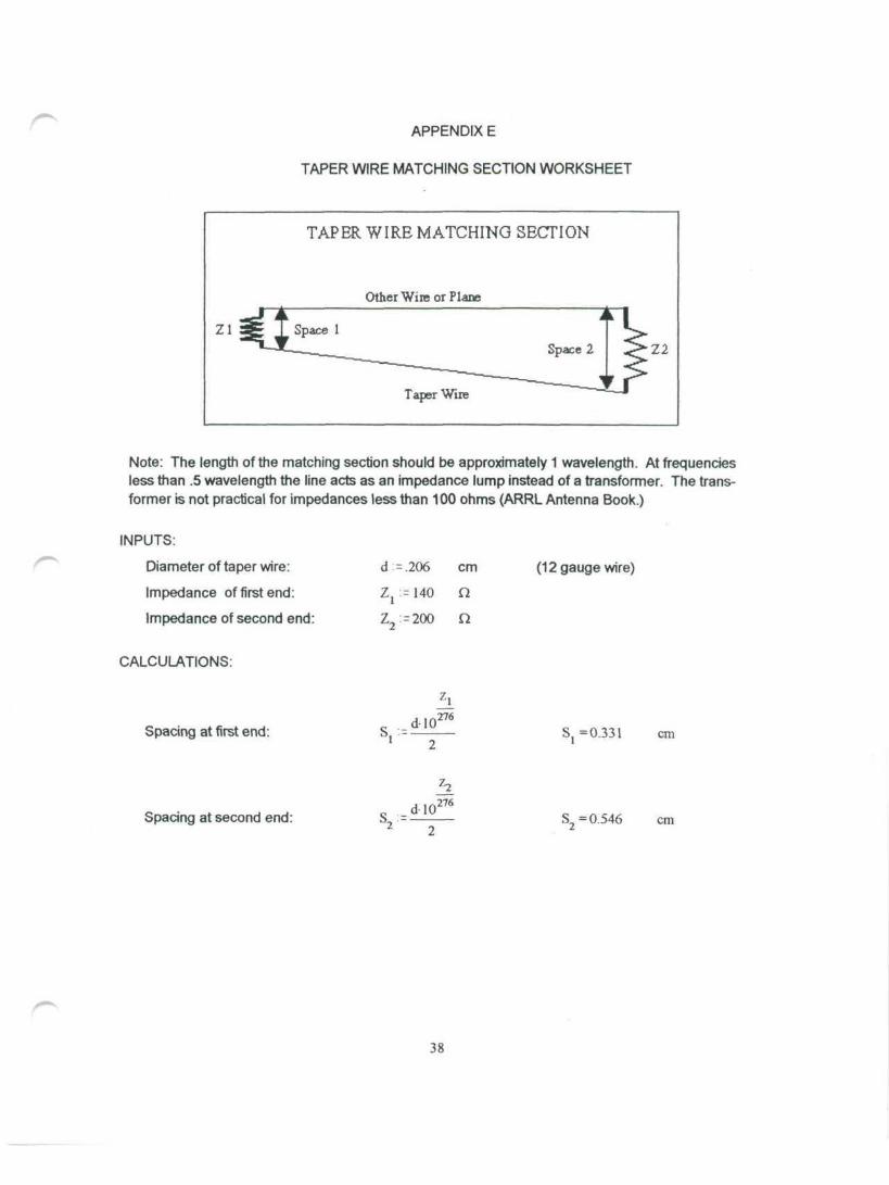
APPENDIX E
TAPER WIRE MATCHING SECTION WORKSHEET
TAPER WIRE MATCHING SECTION
Other Wire or Plane
Taper Wire
Note: The length of the matching section should be approximately 1 wavelength. At frequenciesless than .5 wavelength the line acts as an impedance lump instead of a transformer. The trans-former is not practical for impedances less than 100 ohms (ARRL Antenna Book.)
INPUTS:
Diameter of taper wire:
Impedance of first end:
Impedance of second end:
CALCULATIONS:
d =.206
Z, :=140
cm
Q
n
(12 gauge wire)
Spacing at first end:d l O276
S, =0.331 cm
Spacing at second end: d l O276
S2= 0.546 cm
38

^ APPENDIX F
RECEIVER SENSITIVITY WORKSHEET
INPUTS:
Frequency:
Effective Area of Antenna:
Minimum Signal Intensity:
Predetection Bandwidth:
Detected Signal to Noise Ratio:
Antenna Impedance:
F:=408-1(T Hz
AE =5.797 square m
S =10 Janskys
B := 150000 Hertz
SNR:=.01
Z := 140 Ohms
^
CALCULATIONS:
Antenna Power:
Required Receiver Sensitivity:
PA:=SAE-B 10"
RS: =9.091-
SNR
PA=8.6%'10
RS =3.172
2° Watts
APPENDIX G
RECEIVER DESCRIPTION
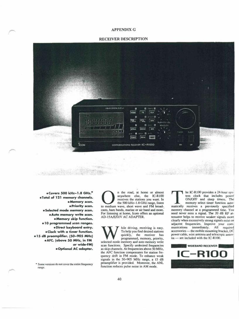
• Covers 500 kHz-1.8 GHz.*•Total of 121 memory channels.
• Memory scan.• Priority scan.
• Selected mode memory scan.•Auto memory write scan.
• Memory skip function.• 10 programmed scan ranges.
• Direct keyboard entry.• Clock with a timer function.
• 15 dB preamplifier. (50-905 MHz)• AFC. (above 50 MHz, in FM
or wide-FM)• Optional AC adapter.
* Some versions do not cover the entire frequencyrange.
O n the road, at home or almostanywhere else, the IC-R100receives the stations you want. Inthe 500 kHz-1.8 GHz range, listen
to medium wave, short wave and FM broad-casts, ham bands, marine or air band and more.For listening at home, Icom offers an optionalAD-15A/E/D/V AC ADAPTER.
w hile driving, receiving is easy.To help you find desired stationsquickly, the receiver hasprogrammed, memory, priority,
selected mode memory and auto memory writescan functions. Specify undesired frequenciesas skip channels. At frequencies above 50 MHz,the AFC function compensates for station fre-quency drift in FM mode. To enhance weaksignals in the 50-905 MHz range, a 15 dBpreamplifier is provided. Moreover, the ANLfunction reduces pulse noise in AM mode.
T he IC-R100 provides a 24-hour sys-tem clock that includes powerON/OFF and sleep timers. Thememory select timer function auto-
matically receives a previously specifiedmemory channel at a programmed time. Youneed never miss a signal. The 20 dB RF at-tenuator helps to receive weaker signals moreclearly when excessively strong signals exist onadjacent frequencies. Improve your com-munications immediately. All requiredaccessories — the mobile mounting bracket, DCpower cable, wire antenna and telescopic anten-na — are included with the IC-R100.
WIDEBAND RECEIVER
IC-R1OO
40

Frequency scoverage*•Varies acconSng to version.
Guaranteed
Operation
Modes-
Sensitivity*-•Each receiver's sensitivity is toes than;, described value. 10 dB S/N.for SS8,sCW.'FSK <RTTY) and AM ..modes. ''.*£-' ,12 dB SINAD for FM and Wido-FM :
i .modes.;-~:
slectivity
Frequency stability
Tuning steps,
Usable antenna connectors.
Dimensions*•Projections riot Included.
Weigh
IC-R100500 kHz-1800 MHz
100 kHz-1856 MHz
AM. FM, Wide-FM
0.5-1.6295 MHzAM 3.2 uV
1 63-49.9995 MHzAM 1.6nVFM 0.56 (iV
50-904.9995 MHzAM 0.56 (iVFM 0.2 (iVWide FM 0.63 (iV
905-1380.4875 MHzFM 0.32 uV
1380.5-1800 MHzFM 0.45 |iV
AMMora than 6.0 kHz/-6 dB
FMMore than 15 kHz/-6 dB
WkJeFMMore than 180 kHz/-3 dB
1, 5. 8, 9, 10, 12.5. 20 or 25 kHz(Varies according to frequency range.)
Below 50 MHz; PL-259Above 50 MHz: Type N
150(W)xSO(H)x181(D)r5.9(W)x2.0(H)x7.1(D)ir
1.4 kg; 3.1 Ib
41
APPENDIX H
A/D CONVERTER DESCRIPTION
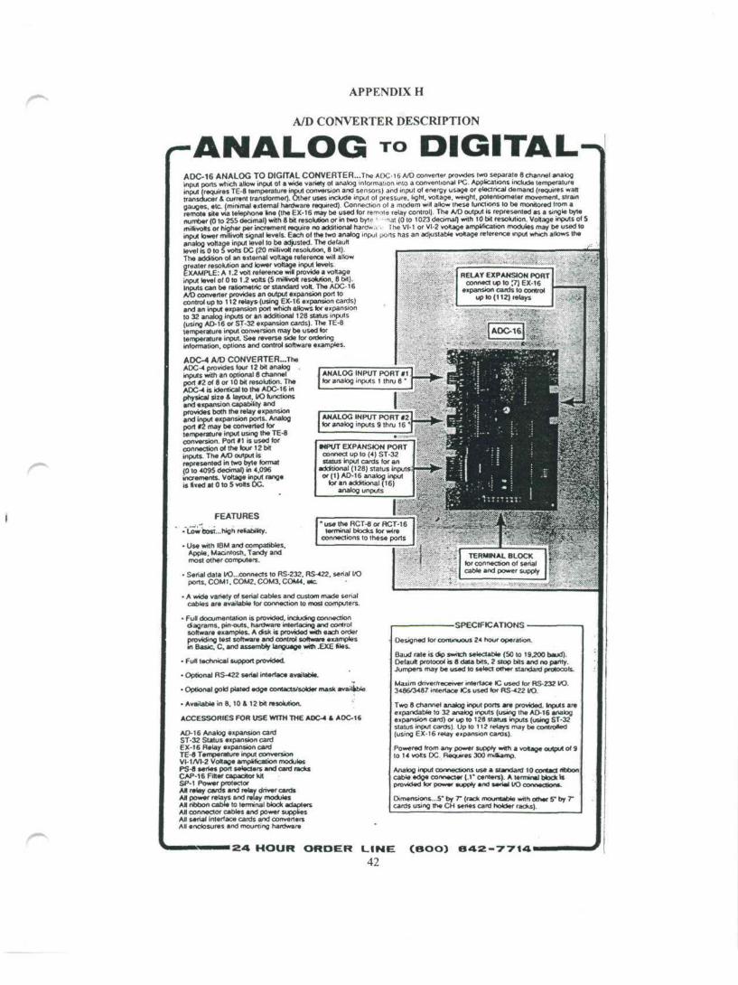
r-ANALOG TO DIGITALADC-16 ANALOG TO DIGfTAL CONVERTER...The ADC-16 A/O converter rxovxles two separate 8 channel analoginput ports which allow input ot a wide variety ol analog information mlo a conventional PC. Applications include temperatureinput (requires TE-8 temperature input conversion and sensors) and inpul of energy usage of electrical demand (requires walltransducer & current transformer). Other uses include inpul ol pressure, light, voltage, weight, potentiometer movement, straingauges etc (minimal external hardware required). Connection ol a modem win allow these (unctions lo be monitored Irom aremote cite via telephone line (the EX-16 may be used lor remote relay control) The A/D output it represented as a single bylenumber (0 to 255 decimal) with 8 bit resolution or in two byle -ial (0 lo 1023 decimal) with 10 bit resolution. Voltage inputs ol Smillivolts or higher per increment require no additional harOw., . rhe VI-1 or VI-2 voltage ampkficalion modules may be used loinput tower millivolt signal levels. Each ol the two analog input ports has an adjustable voltage relerence input which allows theanalog voltage input level lo be adjusted. The defaultlevel is 0 to 5 volts DC (20 millivolt resolution, 8 oil).The addition ol an external voltage reference will allowgreater resolution and tower voltage input levels.EXAMPLE: A 1.2 volt relerence win provide a voltageinput level ol 0 to 1.2 volts (5 miHrvoH resolution. 8 bit).Inputs can be ratkxnetric or standard volt The ADC -16A/O converter provides an output expansion port tocontrol up to 112 relay*(using 6X-16 expansion cards)and an input expansion port which allows lor expansionto 32 analog inputs or an additional 128 status inputs(using AO-16 or ST-32 expansion cards). The TE-8temperature input conversion may be used fortemperature input. See reverse side for orderinginformation, options and control software examples.
ADC-4 A7D CONVERTER...TheADC-4 provides lour 12 bit analoginputs with an optional 8 channelport 92 ol 8 or 10 bit resolution. TheAOC-4 is identical to the ADC-16 inphysical size * layout. I/O functionsand expansion capability andprovides both the relay expansionand input expansion ports. Analogport 12 may be converted lortemperature input using the TE-8conversion. Port 41 is used forconnection ot the (our 12 bitinputs. The A/D output isrepresented in two byte format(0 to 4095 decimal) in 4.096increments. Voltage inpul rangeis fixed at 0 to 5 volts DC.
RELAY EXPANSION PORTconnect up to 7) EX-16
expansion cards lo controlup to (112) relays
ANALOG INPUT PORT *1lor analog inputs 1 thru 8 *
ANALOG INPUT PORT Klor analog inputs 9 thru 16 '•
«PUT EXPANSION PORTconnect up to (4) ST-32status input cards lor an
additional (128) status inputsor (1) AD-16 analog input
tor «n additional (16)analog unputs
• use the RCT-8 or RCT-16terminal blocks lor wire
connections to these ports
FEATURES
•"Low Bo«...high reliability.
• Use with IBM and compatibles.Apple. Madniosh. Tandy andmost other computers.
• Sehal data lO...connects lo RS-232. RS-422. serial I/Oports. COM!. COM2. COM3. COM4. etc.
• A wide variety of serial cables and custom made serialcables are available for connection to most computers.
• Full documentation is provided, including connectiondiagrams, pin-outs, hardware interlacing and controlsoftware examples. A disk is provided with each orderproviding lest software and control software examplesm Basic. C. and assembly language with .EXE ties.
• Fun technical support provided
• Optional RS-422 serial interface available.
• Optional gold plated edge contacts/solder mask available
• Available in 8.10 i 12 bit resolution.
ACCESSORIES FOR USE WITH THE AOC-« t AOC-1S
AD-16 Analog expansion cardST-32 Status expansion cardEX-16 Relay expansion cardTE-6 Temperature input conversionVI-1/VI-2 Voltage amplification modulesPS -8 series port »<eclers and card racksCAP-16 Filter capacitor kitSP-1 Power protectorAM relay cards and relay driver cardsAll power relays and relay modulesAll ribbon cable to terminal block adaptersAll connector cables and power suppliesAll serial interface cards and convertersAll enclosures and mounting hardware
TERMINAL BLOCKtor connection ol serialcable and power supply
-SPECIFICATIONS •
Designed for continuous 24 hour operation.
Baud rale is dip switch selectable (50 to 19.200 baud).Default protocol is 8 data bits. 2 stop bits and no parity.Jumpers may be used to select other standard protocols.
Maxim driver/receiver interface 1C used lor RS-232 LO3486/3487 interface Cs used lor RS-422 IAD.
Two 8 channel analog input ports are provided. Inputs areexpandable lo 32 analog inputs (using the AD-16 analogexpansion card) or up to 128 status inputs (using ST-32status input caros). Up to 112 relays may be controlled(using EX-16 relay expansion cairls).
Powered from any power supply wirh a voltage output ol 9to 14 vofls DC. Requires 300 rmKamp.
Analog input comecuxis use a standard 10 contact ribboncable edge connecter (.1* centers). A terminal block Isprovided lor power supply and serial I/O connection*.
Dimensions...5" by 7~ (rack mountabte with other 5" by 7~cards using the CH series card holder racks).
>24 HOUR ORDER LINE
42(BOO) 842-77141

VOLTAGE AMPLIFICATION MODULES
VI-1 VOLTAGE AMPLIFICATION MODULE...The VM voltage ampirficalton module will amplify tower signal levels (orinput miolhe ADC-16 ANALOG TO OK31TAL CONVERTER The VI-1 module converts a rrwHivort input (0 to 100 miWivo't typtcal)to a 0 to 5 volt DC output (or direct input into one ot the 16 analog inputs on Ihe AOC-16 analog lo digital converter or AD-16expansion card A calibration adjustment is provided to set input scale (down to the 0 10 5 millivolt range). A terminal block isprovtded on the Vl-l (or connections to the power supply ar>d signal I/O. Typical use may include the input ot erwyy usage Iroma watt transducer, the input of weight from a strain cell or the input of pressure trom a pressure transducer Requires 12 voUpower supply. lOOrmlliamp Conned lo the ADC 16 with the RCT-8 terminal block.VI-2 VOLTAGE AMPLIFICATION MODULE...The VI-2 is a iwo channel version ot me VI-1 described above. (2) inputchannels are provided tor ouipui to any (2) AOC-16 analog inputs.
————•ADC-IS ANALOG; TO DIGITAL PACKAGE a—.aa.—
PAC-B ANALOG TO DIGITAL PACKAGE... The AOC-16 analog lo digital package is an assembled package whichincludes a 10" by 7 1/2" plastic enclosure, the ADC-16 analog lo digital converter, the RTC-16 terminal block, power supply andconnecter cable. The serial cable supplied will be the CC-OB25S unless specified otherwise.
(CONTROL SOFTWARE'
CONTROL SOFTWARE FOR THE AOC-16 ANALOG TO DIGITAL CONVERTER
The analog information is transmitted trom the ADC-16 upon request Irom the computer. To initiate the sequence, the A/O chan-nel code must be transmted by the computer. This is accomplished by using the command: PRINT f 1. CHR$(X): (X » I -channel t. channel 1 » 0. channel 2.1. etc.). This command is then repealed (eicept when sequencing) lo initiate transmissionfrom the ADC-16. The ADC-16 will then transmit a number from 0 to 255 to represent the analog information (0-0 voltage, 255« lull scale voltage. 128 - hall scale voltage, etc.). The AOC-16 recognizes only the control codes 0 to 15 (or 0 lo 31 with the AO-16 or ST-32 connected). The ADC-16 passes all higher control codes to the EX-16 (if attached) for relay (unctions.
SAMPLE PROGRAM
The lollowing program w* continuously display Ihe analog information from each of In* 16 analog channels. Tne acraen is up-dated continuously so that new analog information is displayed at intervals onr̂ a lew rnKseconds apart. (GW Basic. IBM tcompatibles)
10CLS20 DIM AJ(20) ...specify array30 OPEN -COM1:96OO.N.8.2.DS.CO.CS- AS »1 ...configure serial port40 FOR X-0 TO 1650 IF X-8 THEN Z-OX3OTO 80 ...synchronize60 IF X-16 THEN Z.15GOTO 8070Z-.X80 PRINT *1 ,CHR$(Z); ...transmit90A$(X).INPuT$(l.l) ..receive NEED HELP WITH SOFTWARE? .100NEXTX / contact us tor technical support110 LOCATE,1.1 or us* our custom aoftwar*120FORX-1 TO 16 '7-\130 PRINT ASC(A$(X));' • ...print on screen140 NEXT XISO GOTO 40
More detailed information is provided with the documentation supplied with the AOC-16.
——«—.———ORDERING INFORMATION.———-.-————
Options lor the ADC-4. ADC-8 I ADC-16 may be ordered by adding the proper sufli« The following options may be entered lorthe Analog to Digital Conveners:
/A Option: Serial I/O is configured lor the RS-422 interface (distances to 4.OOO (Ml. tor us* with the AOC-4. AOC-4 * AOC-16).
IB Option: Alt ribbon cable edge connecter contacts are gold plated ana a solder mask is applied lo tne circuit board surface toinsulate the conductive circuit runs. Gold plated edge contacts may be desired if the nbbon cables are connected and removedfrequently or rt extenled life of the contacts is desired. The solder mask *J reduce the poss»t»tty ol m circuit malfunction causedby foreign metal particles and short circuits.
If. Option: Port* I on the AOC-16 is configured for temperature input (-78* to t 46* F) using the TE-« temperature inputconversion (for use with the AOC-8. AOC-16 » AD-16). Includes e temperature sensors, e trimmers and terminal block.
If Option: Port «2 is configured tor temperature input (same as above, tor use with the AOC 4/1. AOC-16 ft AD-16)
/G Option: Port ft is configured lor 10 bit resolution (for use with the ADC-8. AOC-16 1 AO-16).
/M Option: Port »2 is configured for 10 bit resolution (for use with the AOC-4/1. AOC-16t AO-16).
/I Option: Optional eight channel analog input port *2 added (lor use with the AOC-4)
fZ Option: This option is for use with customized hardware. A 6 digit code will loNow the Z suffix to identify the customer andtype ol modification.
PLEASE NOTE: The AOC-4. AOC-8 t AOC-16 require a power supply, connecter cable and terminal Mock to fcnckon. Selectthe proper cable, power supply and terminal block lor your application and computer from the enclosed data thaetx. The EX-16.AD-16 and ST-32 e«pansion cards require the RC-20 nbbon connecter (sold separate )̂ tor connection 10 the A/O convolat. •
To order Ihe standard AOC-16 analog to digital convener, specify part number AOC-16. The standard ADC-16 w* be cupptedwith an RS-232 serial interface and tin plated edge contacts
To order an-/ of the above options, add me proper surfrv lo the part number. Any number of options may be included by •ddKYgthe proper suffix to the pan number
use AOC-8/E ... toorder the ADC-6 witn pon f t configured kx lemperaturvinput.use ADC 4/A/l to order the ADC-4 wuh HS-422 and Ihe optional 8 bit port t2.use AOC-16/A/EyF to order the ADC-16 with RS-422 and ports tl & K configured tor temperature »iout
i 24 HOUR ORDER LINE (BOO) 842.7714
43

SELECTED BIBLIOGRAPHY
ARRL. 1991. The ARRL Antennfl Book. 16th ed. Newington, CT: i iie American Radio Relay League.
DeMaw, Doug. 1988. The ARRL Electronics Data Book. Newington, CT: The American Radio RelayLeague.
Heiserman, Dave. 1975. Radio Astronomy. Blue Ridge Summit, Pa: Tab Books, Inc.
Hyde, Frank W. 1963. Radio Astronomy for Amateurs. New York: Norton & Company.
King, Howard E. and Jimmy L. Wong. 1984. Helical Antennas. In Antenna Engineering Handbook, ed.Richard C. Johnson and Henry Jasik, Chap. 13. New York: McGraw-Hill Publishing Company.
Kraus, John D. 1984. Electromagnetics. 3ded. New York: McGraw-Hill Publishing Company.
. 1984. Radio-Telescope Antennas. In Antenna Engineering Handbook, ed. Richard C. Johnsonand Henry Jasik, Chap. 41. New York: McGraw-Hill Publishing Company.
Shields, John Potter. 1986. The Amateur Radio Astronomer's Handbook. New York: Crown Publishers, Inc.
Sickels, Robert M. 1992. Radio Astronomy Handbook. 4th ed. Fort Pierce, Florida: Bob's Electronic Service.
. 1992. The Radio Astronomy Circuit Cookbook. Fort Pierce, Florida: Bob's Electronic Service.
44