Embed Size (px)
Citation preview
The Capital Asset Pricing Model (CAPM)
Tee KilenthongUTCC
c⃝Kilenthong 2017
Tee Kilenthong UTCC The Capital Asset Pricing Model (CAPM) 1 / 38
Main Issues
What is an equilibrium implication if all investors construct portfoliosas we studied?
How should we measure risk of any asset?
Tee Kilenthong UTCC The Capital Asset Pricing Model (CAPM) 2 / 38

CAPM: Simple Derivation
The efficient frontier without riskless asset.
Tee Kilenthong UTCC The Capital Asset Pricing Model (CAPM) 3 / 38

CAPM: Simple Derivation
The efficient frontier with riskless asset. The straight line is called thecapital market line.
Tee Kilenthong UTCC The Capital Asset Pricing Model (CAPM) 4 / 38

CAPM: Simple Derivation
The equation of the capital market line is
Re = RF +Rm − RF
σmσe (1)
where σe is an efficient portfolio on the capital market line.Rm−RF
σmrepresents the market price of risk.
σe represents the amount of risk.
That is,
Expected return = (Market price of risk)× (Amount of risk) (2)
Problem: This equation does not describe equilibrium return onnonefficient portfolios or individual securities.
Tee Kilenthong UTCC The Capital Asset Pricing Model (CAPM) 5 / 38

Only Ri and βi Matter
From Single-Index Model, the investor should hold a verywell-diversified portfolio. Therefore, only relevant risk is systematicrisk measured by β.
The only dimensions of a security that need be of concern areexpected return Ri and βi .
Tee Kilenthong UTCC The Capital Asset Pricing Model (CAPM) 6 / 38

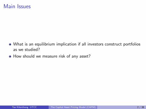
Nonefficient Portfolios and Arbitrage Opportunity
From the above figure, one can imagine that they can make moneyfrom the following arbitrage strategy:
Cash Invested Expected Return β
Portfolio C -100 -11 -1.2Portfolio D +100 +13 +1.2Arbitrage Portfolio 0 2 0
Note: we use βP =∑
i Xiβi .
Main point: there is a portfolio involving zero risk and zero netinvestment that has a positive expected return. There is an arbitrageopportunity. This should not be the case in an equilibrium.
Tee Kilenthong UTCC The Capital Asset Pricing Model (CAPM) 7 / 38
Nonefficient Portfolios and Arbitrage Opportunity
Therefore, all investors must hold efficient portfolios.
Tee Kilenthong UTCC The Capital Asset Pricing Model (CAPM) 8 / 38
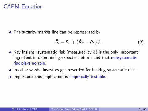
CAPM Equation
The security market line can be represented by
Ri = RF +(Rm − RF
)βi (3)
Key Insight: systematic risk (measured by β) is the only importantingredient in determining expected returns and that nonsystematicrisk plays no role.
In other words, investors get rewarded for bearing systematic risk.
Important: this implication is empirically testable.
Tee Kilenthong UTCC The Capital Asset Pricing Model (CAPM) 9 / 38

CAPM Equation: Alternative
We can represent risk by covariance of asset return and market return:
Ri = RF +
(Rm − RF
σm
)σimσm
(4)
where we use βi =σimσ2m.
Tee Kilenthong UTCC The Capital Asset Pricing Model (CAPM) 10 / 38

CAPM: A More Rigorous Derivation
Recall: an optimal condition for an efficient portfolio is
Rk − RF = λ (X1σ1k + . . .+ XNσNk) (5)
where σki = Cov (Rk ,Ri ).
Homogeneous expectation implies that the solution to this problem orthe optimal portfolio here must be the market portfolio. As a result,
Rm =N∑i=1
RiXi (6)
Then, we can show that
X1σ1k + . . .+ XNσNk = Cov (Rk ,Rm) . (7)
Tee Kilenthong UTCC The Capital Asset Pricing Model (CAPM) 11 / 38

CAPM: A More Rigorous Derivation
So, we can write
Rk − RF = λCov (Rk ,Rm) (8)
Since the market portfolio is one of an efficient portfolio, we can write
Rm − RF = λCov (Rm,Rm) = λσ2m =⇒ λ =
Rm − RF
σ2m
(9)
Finally we can get the CAPM:
Rk − RF =Rm − RF
σ2m
σkm =(Rm − RF
) σkmσ2m
Ri − RF =(Rm − RF
)βi (10)
Tee Kilenthong UTCC The Capital Asset Pricing Model (CAPM) 12 / 38

Keys Assumptions for the Derivation of CAPM
1 No transaction costs, no personal income taxes.
2 Perfect competition.
3 Assets are infinitely divisible.
4 Investors have mean-variance preferences.
5 There exist a riskless asset.
6 Homogeneous expectation.
Tee Kilenthong UTCC The Capital Asset Pricing Model (CAPM) 13 / 38
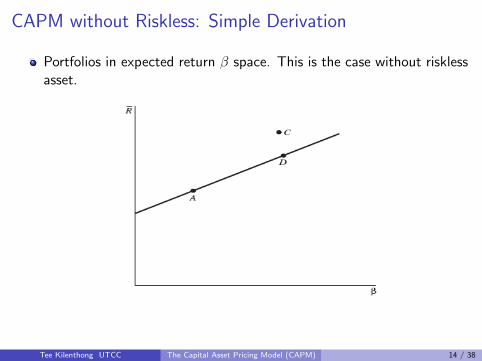
CAPM without Riskless: Simple Derivation
Portfolios in expected return β space. This is the case without risklessasset.
Tee Kilenthong UTCC The Capital Asset Pricing Model (CAPM) 14 / 38
CAPM without Riskless: Simple Derivation
First, combinations of two risky portfolios lie on a straight lineconnecting them in expected return β space.
Second, consider C and D. Using an arbitrage argument as before, wecan show that all portfolios and securities must plot along the straightline, as in the figure.
This line can be represented by
Ri = a+ bβi (11)
Our job is to find what are a and b?
Tee Kilenthong UTCC The Capital Asset Pricing Model (CAPM) 15 / 38
CAPM without Riskless: Simple Derivation
Let RZ be the expected return on a zero beta portfolio. This portfoliomust also be on the straight line:
RZ = a+ b × 0 =⇒ a = RZ (12)
Again, the market portfolio must be on the line as well:
Rm = RZ + b =⇒ b = Rm − RZ (13)
Hence, we have an alternative CAPM (without riskless asset):
Ri = RZ +(Rm − RZ
)βi (14)
Tee Kilenthong UTCC The Capital Asset Pricing Model (CAPM) 16 / 38

CAPM without Riskless: A Rigorous Derivation
Recall: an optimal condition for an efficient portfolio is
Rk − R ′F = λ (X1σ1k + . . .+ XNσNk) (15)
Tee Kilenthong UTCC The Capital Asset Pricing Model (CAPM) 17 / 38
CAPM without Riskless: A Rigorous Derivation
Using the result we derived earlier,
X1σ1k + . . .+ XNσNk = Cov (Rk ,Rm) , (16)
we can write
Rk − R ′F = λCov (Rk ,Rm) (17)
We then can show that
Ri = R ′F +
(Rm − R ′
F
)βi (18)
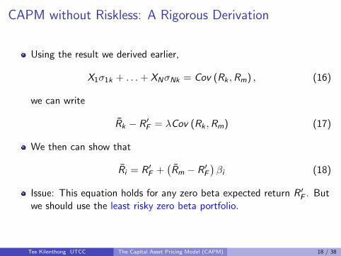
Issue: This equation holds for any zero beta expected return R ′F . But
we should use the least risky zero beta portfolio.
Tee Kilenthong UTCC The Capital Asset Pricing Model (CAPM) 18 / 38
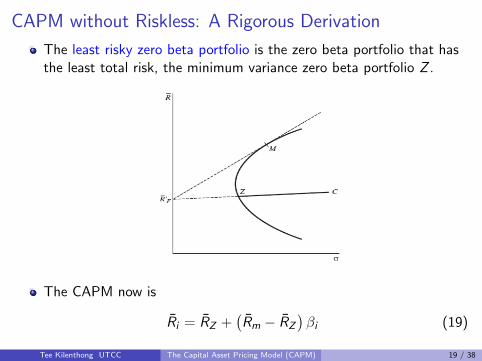
CAPM without Riskless: A Rigorous Derivation
The least risky zero beta portfolio is the zero beta portfolio that hasthe least total risk, the minimum variance zero beta portfolio Z .
The CAPM now is
Ri = RZ +(Rm − RZ
)βi (19)
Tee Kilenthong UTCC The Capital Asset Pricing Model (CAPM) 19 / 38
Overvalued and undervalued
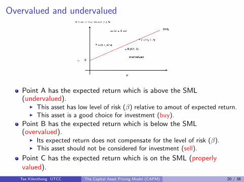
Point A has the expected return which is above the SML(undervalued).
I This asset has low level of risk (β) relative to amout of expected return.I This asset is a good choice for investment (buy).
Point B has the expected return which is below the SML(overvalued).
I Its expected return does not compensate for the level of risk (β).I This asset should not be considered for investment (sell).
Point C has the expected return which is on the SML (properlyvalued).
Tee Kilenthong UTCC The Capital Asset Pricing Model (CAPM) 20 / 38
Testing CAPM
Tee Kilenthong UTCC The Capital Asset Pricing Model (CAPM) 21 / 38

Main Issues
How can we test CAPM model?
Are those tests reliable?
Tee Kilenthong UTCC The Capital Asset Pricing Model (CAPM) 22 / 38
CAPM is in an Ex-ante Form
The basic CAPM model can be written as
E (Ri ) = RF + βi [E (Rm)− RF ] (20)
If lending and borrowing at the risk free rate is not possible or there isno risk free rate, then the CAPM becomes
E (Ri ) = E (RZ ) + βi [E (Rm)− E (RZ )] (21)
Notice: these models are in an expectation form. This is suppose tobe about future values.
An expectation means that we are thinking about the situation beforethe uncertainty is realized. We call this ex-ante.
Tee Kilenthong UTCC The Capital Asset Pricing Model (CAPM) 23 / 38

CAPM is tested using Ex-post Data
On the other hand, we usually perform tests of CAPM models usingrealized (historical) data. These values are said to be ex-post values.How can we justify using ex-post data to test ex-ante model?
Defense: using the law of large number, we should be able toestimate consistently (unbiased) the ex-ante expectation using samplemean of ex-post data.
Tee Kilenthong UTCC The Capital Asset Pricing Model (CAPM) 24 / 38
Ex-post test of Ex-ante CAPM model
That is, testing a CAPM model is a simultaneous test of all threefollowing hypothesises:
1 The market model holds2 The CAPM model holds3 βi is stable over time
NOTE: if there is no risk free rate, we will test the following model
Rit = RZt + βi
[Rmt − RZt
]+ eit (22)
Tee Kilenthong UTCC The Capital Asset Pricing Model (CAPM) 25 / 38

Simple Test of CAPM
Sharpe and Cooper (1972) divide stocks into ten portfolios using betaas a criterion. β at each point in time uses past 60 months of data.They also calculate average returns of each portfolio.
They then estimate a linear equation
Ri = 5.54 + 12.75βi (23)
with R2 > 0.95.
Key Points: the relationship between return and β is linear. Thoughthe intercept (supposed to represent the risk free rate) is too high.
Tee Kilenthong UTCC The Capital Asset Pricing Model (CAPM) 26 / 38
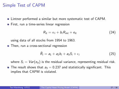
Simple Test of CAPM
Lintner performed a similar but more systematic test of CAPM.
First, run a time-series linear regression
Rit = αi + biRmt + eit (24)
using data of all stocks from 1954 to 1963.
Then, run a cross-sectional regression
Ri = a1 + a2bi + a3Si + ϵi (25)
where Si = Var(eit) is the residual variance, representing residual risk.
The result shows that a3 = 0.237 and statistically significant. Thisimplies that CAPM is violated.
Tee Kilenthong UTCC The Capital Asset Pricing Model (CAPM) 27 / 38

More Advanced Test of CAPM
Miller and Scholes TestI If the CAPM is the right model, then βi from the following equation
should be consistent
Rit = (1− βi )RFt + βi Rmt (26)
I If RFt is constant over time, there will no problem. But it is not thecase in general. Hence, there should be an estimation biased.
I Perhaps the relationship is nonlinear. But they found that it is not thatimportant.
I Heteroscedasticity. Again they found that it is not that important.I Measurement error in βi . They found that this is significant.
Tee Kilenthong UTCC The Capital Asset Pricing Model (CAPM) 28 / 38

More Advanced Test of CAPM
Black, Jensen, and Scholes TestI They first run the following time-series regression
Rit − RFt = αi + βi (Rmt − RFt) + eit (27)
I If CAPM generates the return data, then α = 0.I They second run a cross-sectional regression of CAPM and found that
Ri − RF = 0.00359 + 0.01080βi (28)
I This result supports the CAPM.
Tee Kilenthong UTCC The Capital Asset Pricing Model (CAPM) 29 / 38

Fama and MacBeth Test
They use the same procedure as Black et al. to form 20 portfolios.
The difference is in the cross-sectional regression:1 They run
Rit = γ0t + γ1tβi − γ2tβ2i + γ3tSet + ηit (29)
2 This regression is run each month, month by month. Therefore, theycan study how the parameters change over time.
Tee Kilenthong UTCC The Capital Asset Pricing Model (CAPM) 30 / 38
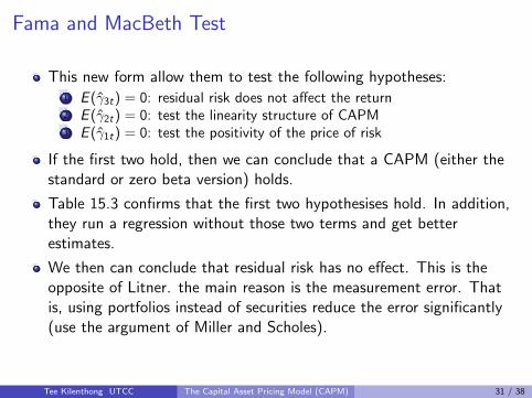
Fama and MacBeth Test
This new form allow them to test the following hypotheses:1 E (γ3t) = 0: residual risk does not affect the return2 E (γ2t) = 0: test the linearity structure of CAPM3 E (γ1t) = 0: test the positivity of the price of risk
If the first two hold, then we can conclude that a CAPM (either thestandard or zero beta version) holds.
Table 15.3 confirms that the first two hypothesises hold. In addition,they run a regression without those two terms and get betterestimates.
We then can conclude that residual risk has no effect. This is theopposite of Litner. the main reason is the measurement error. Thatis, using portfolios instead of securities reduce the error significantly(use the argument of Miller and Scholes).
Tee Kilenthong UTCC The Capital Asset Pricing Model (CAPM) 31 / 38
Fama and MacBeth Test
Given that a CAPM holds, then we can further distinguish betweenthe standard and zero-beta CAPM using E (γ0t) and E (γ1t).
If the zero beta model is the true model, the deviation of γ0t from itsmean E (RZ ) and the deviation of γ1t from its mean E (Rm)− E (RZ )must be random.
Since we know that E (RZ ) > RF , if E (γ0t − RF ) > 0 andE (γ1t − E (Rm) + RF ) < 0, we will then conclude that the zero betamodel is the true model.
They find that1 price of risk is positive,2 ¯γ0 is greater than RF and ¯γ1 is less than Rm − RF
These results support the zero beta CAPM.
Tee Kilenthong UTCC The Capital Asset Pricing Model (CAPM) 32 / 38
Fama and MacBeth Test
We can also test if the market operates as a fair game (efficientmarket). If CAPM is a true model, the expected value of γ2t and γ3tat time t + 1 should be zero, regardless of past values.
Fama and MacBeth test this implication by looking at the correlationof γ3t with its lags values. They found that the correlation is notstatistically different from zero. They also found a similar result forγ2t .
They then conclude that the market operates as a fair game.
Tee Kilenthong UTCC The Capital Asset Pricing Model (CAPM) 33 / 38
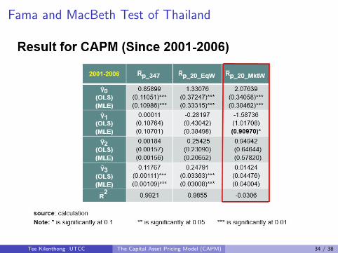
Fama and MacBeth Test of Thailand
Tee Kilenthong UTCC The Capital Asset Pricing Model (CAPM) 34 / 38

Fama and MacBeth Test of Thailand
Tee Kilenthong UTCC The Capital Asset Pricing Model (CAPM) 35 / 38
CAPM is Not Testable?
If any ex-post mean variance efficient portfolio p selected as themarket portfolio, and β are computed using this portfolio as themarket proxy, then
Ri = RZP + βip(Rp − RZP
)(30)
must hold.
That is, testing CAPM is not meaningful.
Tee Kilenthong UTCC The Capital Asset Pricing Model (CAPM) 36 / 38

Roll’s Proof
Consider again the first order condition of an optimal portfolioproblem:
λ (X1σ1k + . . .+ XNσkN) = Rk − RF (31)
Let p be the optimal portfolio, hence we can write
λσkp = Rk − RF (32)
which must be true for any asset or portfolio.
That is, it must be true for the optimal portfolio p as well:
λσ2p = Rp − RF ⇒ λ =
Rp − RF
σ2p
(33)
Hence, we have
Ri = RF +σkp
σ2p
(Rp − RF
)= RF + βkp
(Rp − RF
)(34)
Tee Kilenthong UTCC The Capital Asset Pricing Model (CAPM) 37 / 38
Roll’s Proof
Using a similar argument as before, we can have a model withoutriskless:
Ri = RZp + βkp(Rp − RZp
)(35)
where RZp is the mean return of the minimum varaince zero betaportfolio.
This proves that we can write a zero beta CAPM model with anyefficient portfolio as a market proxy. But the true CAPM is the onewith the true market portfolio.
If we cannot observed the true market portfolio, then we cannot testthe CAPM!
Tee Kilenthong UTCC The Capital Asset Pricing Model (CAPM) 38 / 38