The Canadian Gravimetric Geoid Model 2005 … Canadian Gravimetric Geoid Model 2005 (CGG2005) Marc Véronneau and Jianliang Huang Geodetic Survey Division, Natural Resources Canada,

The Canadian Gravimetric Geoid Model 2005 (CGG2005) Marc Véronneau and Jianliang Huang Geodetic Survey Division, Natural Resources Canada, Ottawa, Ontario, Canada

Abstract: Natural Resources Canada developed a new and enhanced gravimetric geoid model for Canada (CGG2005). As for CGG2000 (previous model), CGG2005 follows the Helmert-Stokes scheme, i.e., the gravity measurements are reduced in terms of Helmert’s second condensation method and the geoid heights are determined using Stokes’s integral. All related reductions to the gravity measurements are determined using the spherical approximation. The main enhancement is the inclusion of satellite gravity data from the GRACE mission. This gravimetric information, obtained from GGM02C (degree and order 200), defines accurately the long wavelength components of the geoid up to degree and order 90 (> ~450 km) by using the degree-banded Stokes kernel. CGG2005 is compared to CGG2000 and the latest US geoid model (USGG2003), and is validated against GPS/Levelling data across Canada and USA. For 2269 benchmarks distributed across Canada’s main land, the mean and standard deviation is -43.4 cm and 13.0 cm, respectively. Part of the misfit can probably be associated with systematic errors in the Canadian primary levelling network. The standard deviation improves to 7.2 cm after removing a systematic trend in the levelling network by using a planar transformation.

Key words: Geoid, Helmert, Stokes, GRACE

1 Introduction The ever-increasing capability to achieve accurate positioning with ease using the Global Positioning System (GPS) increases the demand for a highly accurate geoid model. This demand will continue to increase substantially over the years with the improvement to GLONASS and with the up-coming launch of the GALILEO satellites. These three satellite constellations (GPS, GLONASS and GALILEO) are fundamental components of a Global Navigation Satellite System (GNSS) for accurate horizontal (latitude and longitude) and vertical (height) positioning. Several applications requiring a geometric surface for reference make direct use of the ellipsoid heights derived from GNSS. However, they must be corrected by geoid heights in order to coincide with the elevations on topographical maps, be compatible with benchmarks and be useful to manage water resources properly. Furthermore, the geoid model is becoming an essential component for the realization of a new vertical datum for Canada [Véronneau 2006]. It defines a common and homogeneous reference surface for heights all across the Canadian land mass and surrounding oceans. The current vertical datum, the Canadian Geodetic Vertical Datum of 1928 (CGVD28) [Cannon 1929], is only accessible at a limited number of benchmarks (~80 000), which are mostly located in southern Canada. This limited coverage creates a number of loosely connected local networks in remote regions making data sharing more complex. Furthermore, CGVD28 contains known systematic errors at the regional and national scale that become apparent to users of modern space-based positioning techniques [Véronneau et al. 2001; Véronneau 2006]. The development of an accurate geoid model for a country as vast as Canada is a challenge. The rough relief of the Western Cordillera, the large water basins like Hudson Bay, the Great Lakes and surrounding oceans, the harsh Arctic conditions and the natural motion of the topography due to episodic and secular geodynamics, like earthquakes and postglacial rebound (PGR), make the

The Canadian Gravimetric Geoid Model 2005 (CGG2005)

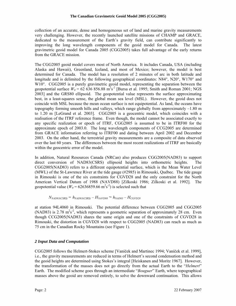
collection of an accurate, dense and homogeneous set of land and marine gravity measurements very challenging. However, the recently launched satellite missions of CHAMP and GRACE, dedicated to the measurement of the Earth’s gravity field, can contribute significantly to improving the long wavelength components of the geoid model for Canada. The latest gravimetric geoid model for Canada 2005 (CGG2005) takes full advantage of the early returns from the GRACE mission. The CGG2005 geoid model covers most of North America. It includes Canada, USA (including Alaska and Hawaii), Greenland, Iceland, and most of Mexico; however, the model is best determined for Canada. The model has a resolution of 2 minutes of arc in both latitude and longitude and is delimited by the following geographical coordinates: N84°, N20°, W170° and W10°. CGG2005 is a purely gravimetric geoid model, representing the separation between the geopotential surface W0 = 62 636 856.88 m2s-2 [Bursa et al. 1995; Smith and Roman 2001; NGS 2003] and the GRS80 ellipsoid. The geopotential value represents the surface approximating best, in a least-squares sense, the global mean sea level (MSL). However, the geoid does not coincide with MSL because the mean ocean surface is not equipotential. As land, the oceans have topography forming smooth hills and valleys, which range globally from approximately –1.80 m to 1.20 m [LeGrand et al. 2003]. CGG2005 is a geocentric model, which coincides with a realisation of the ITRF reference frame. Even though, the model cannot be associated exactly to any specific realization or epoch of ITRF, CGG2005 is assumed to be in ITRF00 for the approximate epoch of 2003.0. The long wavelength components of CCG2005 are determined from GRACE information referring to ITRF00 and dating between April 2002 and December 2003. On the other hand, the terrestrial gravity measurements are a composite of data observed over the last 60 years. The differences between the most recent realizations of ITRF are basically within the geocentric error of the model. In addition, Natural Resources Canada (NRCan) also produces CGG2005(NAD83) to support direct conversion of NAD83(CSRS) ellipsoid heights into orthometric heights. The CGG2005(NAD83) refers to a different equipotential surface, which is the Mean Water Level (MWL) of the St-Lawrence River at the tide gauge (#2985) in Rimouski, Québec. The tide gauge in Rimouski is one of the six constraints for CGVD28 and the only constraint for the North American Vertical Datum of 1988 (NAVD88) [Zilkoski 1986; Zilkoski et al. 1992]. The geopotential value (W0 = 62636859.66 m2s-2) is selected such that NNAD83(CSRS) = hNAD83(CSRS) – HNAVD88 ~ hNAD83 – HCGVD28 at station 94L4060 in Rimouski. The potential difference between CGG2005 and CGG2005 (NAD83) is 2.78 m2s-2, which represents a geometric separation of approximately 28 cm. Even though CCG2005(NAD83) shares the same origin and one of the constraints of CGVD28 in Rimouski, the distortion in CGVD28 with respect to CGG2005 (NAD83) can reach as much as 75 cm in the Canadian Rocky Mountains (see Figure 1). 2 Input Data and Computation CGG2005 follows the Helmert-Stokes scheme [Vaníček and Martinec 1994; Vaníček et al. 1999], i.e., the gravity measurements are reduced in terms of Helmert’s second condensation method and the geoid heights are determined using Stokes’s integral [Heiskanen and Moritz 1967]. However, the transformation of the masses does not go directly from the actual Earth to the “Helmert” Earth. The modified scheme goes through an intermediate “Bouguer” Earth, where topographical masses above the geoid are removed entirely, to solve the downward continuation. This allows

Page: 2 22 February 2007


Figure 1: Distortion in CGVD28 with respect to CGG2005 (hSN3.3d – HCGVD28 – NCGG2005)

the creation of a relatively smooth gravity field easing the instability problem of the downward continuation. Furthermore, the contribution of the downward continuation to the geoid model becomes less than 15 cm in the Western Cordillera and negligible for the rest of the country [Huang and Véronneau 2005]. All terrain-related reductions to the gravity measurements are determined using the spherical approximation [Martinec 1993]. The gravity data for the realization of CGG2005 are basically the same as CGG2000 [Véronneau 2001] with the exception of the global gravity model. CGG2005 makes use of the early results from the GRACE mission. The satellite and surface gravity data are combined by applying the remove-restore technique through Stokes’s integral. The 1D-Fast Fourier Transform [Haagmans et al. 1993] solves the integral. Finally, the geoid model is transformed back to the actual Earth from the “Helmert” Earth by adding the primary indirect effect to the co-geoid. Appendix A describes in details the theory and assumptions for the realization of CGG2005. The recent global gravity model GGM02C [Tapley et al. 2005], degree and order 200, is a spherical harmonic model describing the Earth’s gravity field. It is a combined model made of GGM02S and a global set of surface gravity data. GGM02S is a GRACE-only solution and extends to degree and order 120; thus, it contains gravity information for wavelengths longer than ~300 km. The spherical harmonic coefficients of EGM96 from 201 to 360 are appended to GGM02C to increase the resolution of the global gravity field. The GGM02C/EGM96 model plays two roles. It defines the long wavelength components of the geoid model for North America and complements the terrestrial gravity data outside North America. In addition, the combined model is modified to represent the “Helmert” Earth to further minimize the error coming from outside the integration radius [Vaníček et al. 1995]. On the other hand, the continental surface gravity measurements (land and marine) determine the short wavelength components of the geoid model. CGG2005 contains some 2.2 million gravity



measurements obtained from NRCan, NOAA’s U.S. National Geodetic Survey (NGS), U.S. National Geospatial-Intelligence Agency (NGA) and Denmark’s Kort Matryxkelrysen (KMS). Approximately 65% of these data are over the U.S. territory. The gravity dataset also includes the airborne gravity measurements for Greenland that NRCan received from NGA and KMS. In addition, the shipborne measurements are augmented by a combination of satellite altimetry-derived gravity data determined by Sandwell and Smith [v9.2, 1997], KMS v99 [Andersen and Knudsen 1998], CLS/SHOM v98 and GSFC v2000. All gravity measurements are (or assumed to be) tied to the IGNS71 in a tide-free system. The Digital Elevation Model (DEM) for Canada is from provincial and federal sources. The DEM for the provinces of British Columbia and Alberta is derived from maps at a scale of 1:20k while the DEM for the province of New Brunswick is obtained from maps at a scale of 1:10k. These data are made available to NRCan by the respective provincial agencies. The elevations have a vertical accuracy better than 10 metres and a horizontal resolution of 25 to 100 metres depending on the roughness of the topography. The heights for the rest of Canada are obtained from the Canadian Digital Elevation Data (CDED), which are elevations scanned from maps 1:250k with a horizontal resolution of 3 seconds of arc (~90 m) and a vertical accuracy ranging from 30 metres to 150 metres. For the USA (including Alaska), the original version of the Digital Terrain Elevation Data (DTED) is still used for the realization of the model. This DTED version is of lesser quality than the DEM currently used in the American geoid model USGG2003 [NGS 2003]. The DEM and ice thickness model for Greenland was made available to NRCan by KMS. The elevations for the rest of the world are obtained from GTOPO30. These DEM allowed the determination of terrain corrections at gravity measurement points in Canada. Furthermore, they contribute to the computation of the Mean Helmert anomalies (see appendix A.5) and primary indirect topographical effect (see appendix A.6). Even though the effect of topographical density variation on the geoid model may contribute close to 10 cm [Pagiatakis et al. 2000; Huang et al. 2001] in a few regions of the Western Cordillera, it is not taken into consideration for the realization of CGG2005. CGG2005 uses a constant topographical density of 2.67 g cm-3. The combination of the GGM02C global gravity model and the North American Helmert gravity anomalies is made possible through the Stokes kernel, which is basically a weight function. The original Stokes kernel is modified to filter out the long wavelength components from the surface gravity measurements. It is also truncated to coincide to the resolution of the mean surface gravity data to minimize the aliasing error. These modifications describe the degree-banded Stokes kernel [Huang and Véronneau 2005]. For CGG2005, the degree-banded Stokes kernel is modified to degree 90, i.e., the first 90 degrees (> 450 km) of GGM02C define the long wavelength components. The kernel is also truncated at degree 5400, which represents the resolution of the Helmert gravity anomalies (2’ x 2’). The surface gravity anomalies are integrated for a 6-degree cap radius. The selection of these parameters are based on the analysis of a series of geoid models determined from different degrees of modification (10 to 360), different integration cap-sizes (0.5 to 18 degrees of arc) and different global geopotential models (EGM96 [Lemoine et al. 1998], GFZ97 [Gruber et al. 1997], GRIM5-S1 [Lemoine et al. 1999] and PGM2000A [Pavlis et al. 2000]). For the GRIM5-S1 model, which is a satellite only solution to degree 99 and order 95, the far zone contribution of the geoid model was determined from the EGM96 models. Each solution was compared to geoid heights (N) determined from GPS ellipsoidal heights (h) and geodetic-levelled orthometric heights (H) across Canada: NModel = hGPS – HLev. This independent data set is described in the next section.



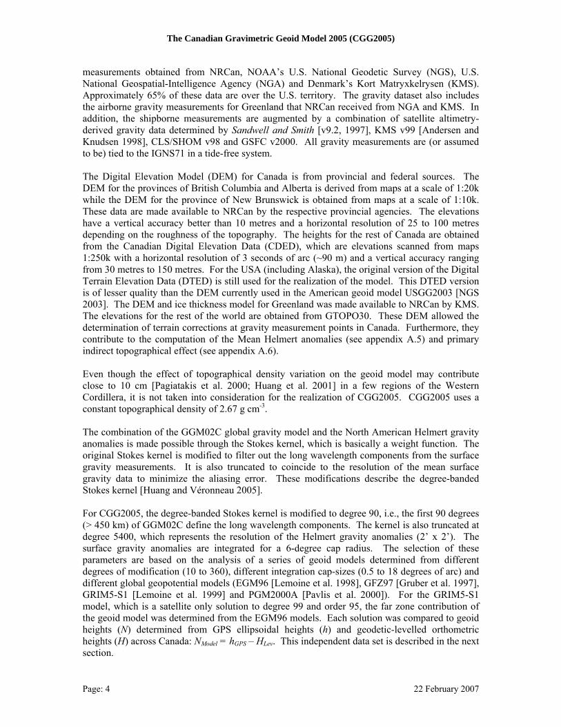
3 Accuracy and independent validation of CGG2005 An estimated accuracy model (66% confidence level) of the CGG2005 geoid model is determined using the Almost Unbias Estimator (AUE) technique [see e.g. Huang et al. 2006]. Its absolute accuracy is depicted in Figure 2. The accuracy ranges from 1 cm to 30 cm. The average error is 3.6 cm with a standard deviation of 2.2 cm. Overall, the estimate of the accuracy is too optimistic because it does not take into consideration the systematic errors above degree 90 in the mean Helmert gravity anomalies derived from the surface gravity measurements, omission errors (e.g., topographical density variation) and theoretical approximation. Even though CGG2005 estimated accuracy may be too optimistic for some regions of Canada, it can still be used as a good indicator of the quality of the geoid model. Naturally, the relative precision of the geoid heights is not represented by the absolute accuracy. For example, the relative precision of the geoid heights in the Western Cordillera could be as good as a few cm for baselines as long as 100 km even though the absolute accuracy of the geoid model reaches the decimetre level. Overall, the long wavelength components (>450 km) of CGG2005, which are determined from GRACE data, have a relative precision of a few centimetres. Similarly, the short wavelength components (<100 km), which are determined from terrestrial gravity data and DEM, have also a precision of a few centimetres. The main weakness in the model most likely lay with wavelength components between 100 km and 450 km where systematic errors may accumulate to reach the decimetre level. The GOCE satellite mission, to be launched in the fall of 2007, may contribute to improving this frequency band.

Figure 2: Absolute accuracy of CGG2005



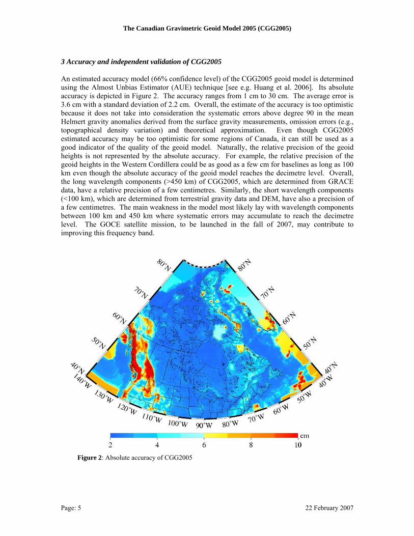
3.1 Validation to GPS/Levelling data Currently, the best independent technique for validating geoid models is to compare their geoid heights (N) to those obtained by differencing GPS ellipsoidal heights (h) and geodetic-levelled orthometric heights (H). The validation can be absolute (h–H–N) or relative (∆h–∆H–∆N). However, the limitation of these two approaches is the difficulty to dissociate the errors coming from the geoid model, GPS observations, levelling measurements, and the stability of benchmarks. The collection of GPS surveys conducted by NRCan across Canada between 1986 and 2003 was assembled and integrated into ITRF97 (epoch 97.0) using the Canadian Base Network (CBN) as the framework [Craymer and Lapelle 1997]. This national network is referred to as GPS Supernet v3.3. Whereas the more recent GPS surveys conducted in 2004, 2005 and 2006 were added to Supernet v3.3 by local adjustments. This updated version is tagged as Supernet v3.3e. Over the years, the GPS surveys used a wide variety of equipment, observing procedures and session lengths (from less than an hour to a few days). Consequently, the adjusted coordinates are of varying precision. The precision of the ellipsoidal heights ranges mostly from a few mm to 10 cm, 95% confidence level. However, there are some older surveys for which the accuracy is a few decimetres; mainly due to the use of single frequency receivers and the mixing of different antennae types (no estimates of the relative phase centre offsets were available). Parts of the 1989 “GPS on BM” project in British Columbia suffered from this problem. In general, the 95% confidence level is a good indicator of the precision of the ellipsoidal heights while the average observation length of each project is a useful indicator of their reliability. The GPS observations are not corrected for systematic errors related to post-glacial rebound. The orthometric heights are determined from a minimum constraint adjustment of geopotential number differences observed by geodetic levelling after 1981. This date marks the beginning of a period when observations we made with our most reliable levelling instruments. The minimum constraint adjustment also includes extra observations from the 1970’s to tie the levelling network between the Atlantic Ocean (Halifax) and Pacific Ocean (Vancouver) and to close a few large levelling loops. Benchmark “7629325” in Rimouski, Québec is held fix at a geopotential number of 4.5933 m2s-2. This represents the potential difference with the mean water level of the St-Lawrence River at the tide gauge #2985 in Rimouski. The remaining levelling observations, which are grouped into three epochs starting from 1971, 1940 and 1904, are added subsequently to the initial adjustment. Each epoch is constrained to the adjusted geopotential numbers of the previous adjustment. This approach is chosen in order to minimize systematic errors coming from post-glacial rebound and older levelling data. Thus, the final adjustment includes four epochs of data starting from 1982, 1971, 1940 and 1904. The adjusted geopotential numbers are divided by mean gravity, which also includes a correction for the topography roughness [Heiskanen and Moritz 1967]. These adjusted orthometric heights are referred to as Jan06. The adjustment indicates that the mean sea level of the Pacific Ocean in the vicinity of Vancouver is higher than the mean sea level of the Atlantic Ocean next to Halifax by 89 cm, whereas the CGG2005 geoid model indicates a difference of 67 cm between the two coasts. Table 1 gives the water level difference between Vancouver and Halifax for different levelling adjustments and geoid models. It shows well the accumulation of systematic errors in the levelling data for different epochs. The adjustment of the geodetic levelling networks for Newfoundland, Prince Edward Island (PEI) and Vancouver Island are conducted in a similar fashion as for the main land. Each network is a minimum constraint to which older observations are added by epoch and constrained to the previously adjusted parameters (geopotential numbers). The stations held fix are 76F703



(84.3050 m2s-2), PE05803 (38.0480 m2s-2) and 87C9766 (5.1608 m2s-2) for Newfoundland, PEI and Vancouver Island, respectively. Table 1. Sea surface topography (SST) and water level difference at tide gauges in Vancouver (V),

Rimouski (R) and Halifax (H) for different adjustments of the primary levelling network and geoid models. The SST is set at 0 cm in Rimouski for all vertical datums.

Sea Surface Topography (cm) ∆SST (cm) Datum

V H R V - H Comments

Adj. 07-28 +35 +12 0 +23 Levelling from 1907 to 1928 Adj. 66-71 +200 -5 0 +205 Levelling from 1966 to 1971 NAVD88 +141 -10 0 +151 North American Adjustment Jan06 +81 -8 0 +89 Levelling from1981 to 2005 CGG2000 +40 +0 0 +40 Geoid Model (Canada) CGG2005 +59 -8 0 +67 Geoid Model (Canada) USGG2003 +64 -4 0 +68 Geoid Model (USA)

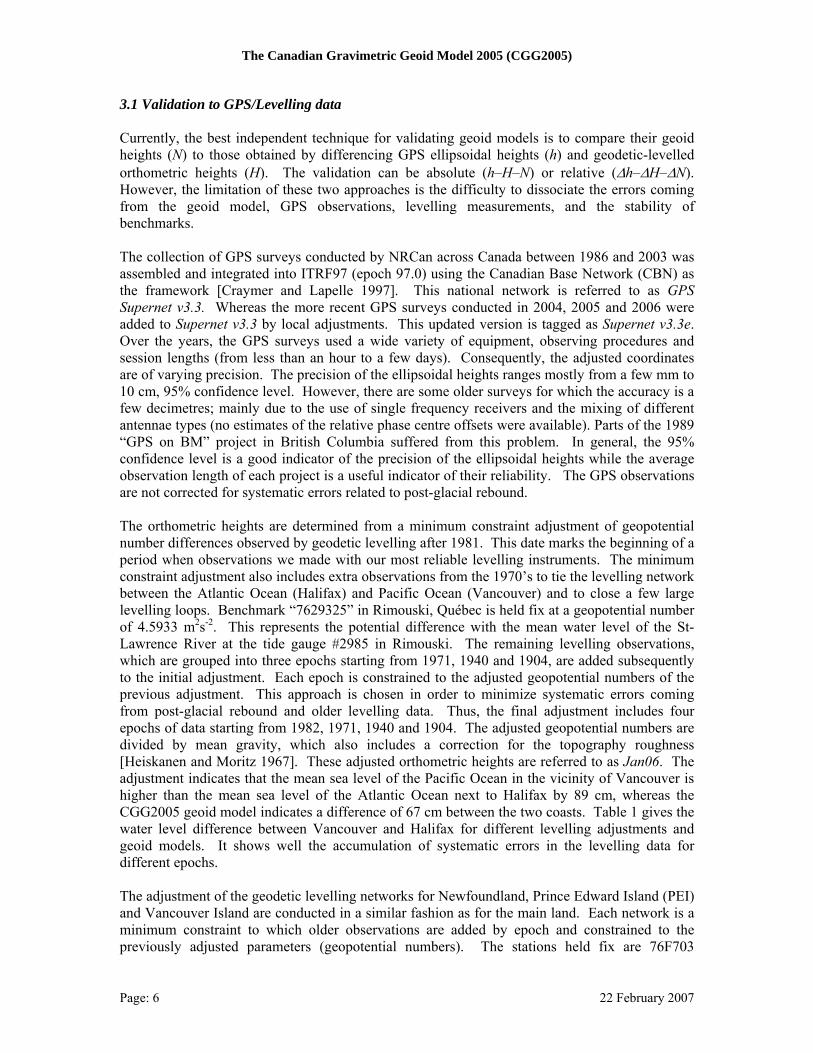
Supernet v3.3e has a total of 3602 stations (Figure 3). Of those, there are 2476 stations with known orthometric heights in the Jan06 adjustment. Thirty-seven (37) of these stations are rejected because their discre-pancies (h-H-N) are significantly larger (e.g., >20 cm) than other discrepancies in the immediate vicinity. Several rejected stations are associated with the 1986 and 1989 GPS surveys around Great Slave Lake in the Northwest Territories and across British Columbia, respectively. The rejected stations also include benchmarks on the levelling lines between Haines Junction, Yukon Territory and Haines, Alaska where the discrepancies (h-H-N) range from -30 cm to +54 cm (see Figure 4). This 220-km segment will be more closely analyzed after collecting new GPS, levelling and gravity data in the summer of 2007. These new data will also allow a better investigation of geoid modeling in areas where gravity measurements are sparse and the topography is rough. Finally, the remaining stations are rejected because they are suspected of being unstable. In some cases, the levelling and GPS surveys were carried out more than 40 years apart. Thus, there are 2439 stations where the ellipsoidal heights and orthometric heights have an acceptable accuracy to validate geoid models across Canada.

Figure 3: Distribution of the GPS stations (red) on benchmarks across Canada

Figure 4: Discrepancies h-H-N in the area of Whitehorse, Yukon



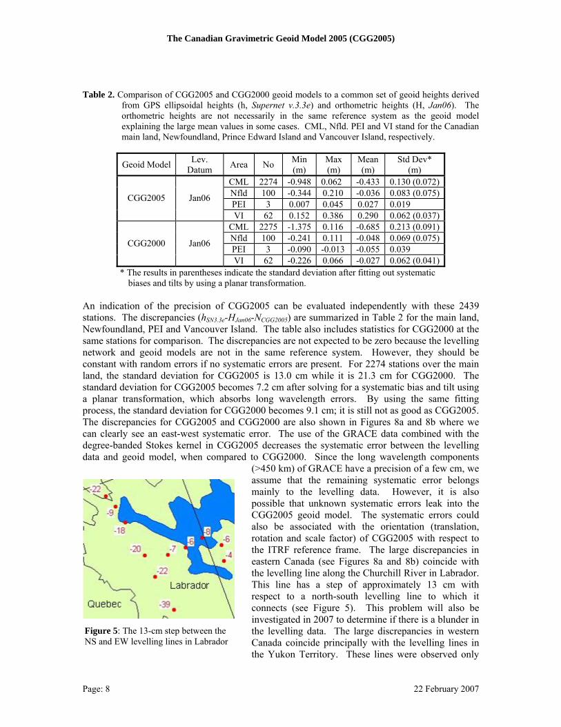
Table 2. Comparison of CGG2005 and CGG2000 geoid models to a common set of geoid heights derived

from GPS ellipsoidal heights (h, Supernet v.3.3e) and orthometric heights (H, Jan06). The orthometric heights are not necessarily in the same reference system as the geoid model explaining the large mean values in some cases. CML, Nfld. PEI and VI stand for the Canadian main land, Newfoundland, Prince Edward Island and Vancouver Island, respectively.

Geoid Model Lev. Datum Area No Min

(m) Max (m)

Mean (m)

Std Dev* (m)

CML 2274 -0.948 0.062 -0.433 0.130 (0.072) Nfld 100 -0.344 0.210 -0.036 0.083 (0.075) PEI 3 0.007 0.045 0.027 0.019

CGG2005 Jan06

VI 62 0.152 0.386 0.290 0.062 (0.037) CML 2275 -1.375 0.116 -0.685 0.213 (0.091) Nfld 100 -0.241 0.111 -0.048 0.069 (0.075) PEI 3 -0.090 -0.013 -0.055 0.039 CGG2000 Jan06

VI 62 -0.226 0.066 -0.027 0.062 (0.041) * The results in parentheses indicate the standard deviation after fitting out systematic

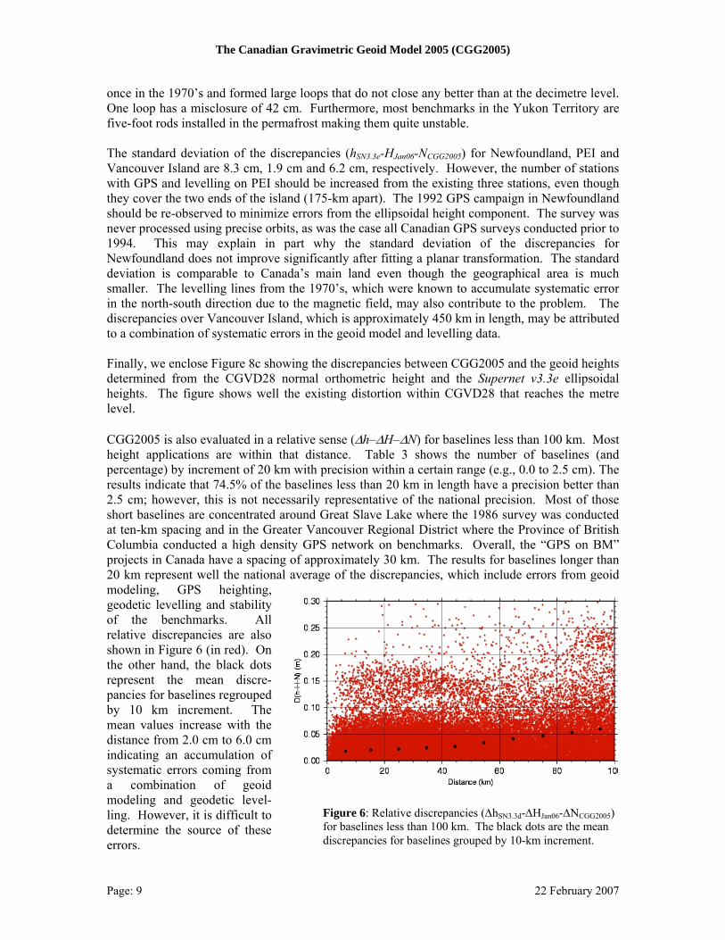
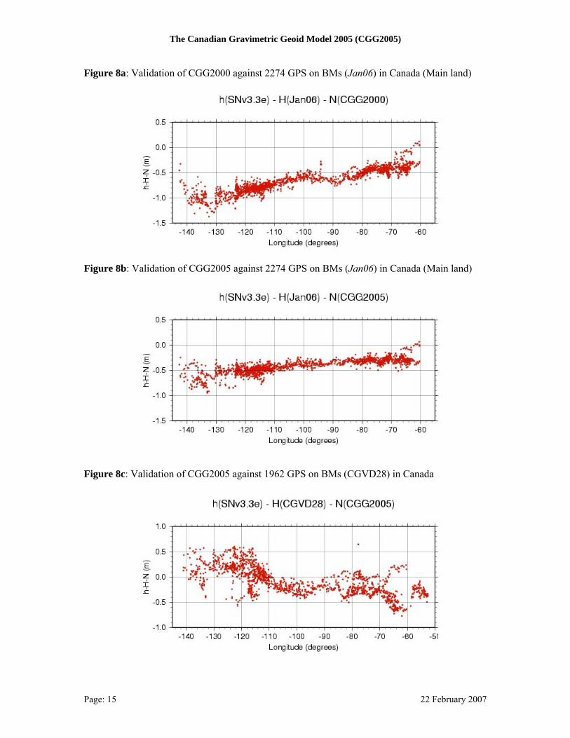
biases and tilts by using a planar transformation. An indication of the precision of CGG2005 can be evaluated independently with these 2439 stations. The discrepancies (hSN3.3e-HJan06-NCGG2005) are summarized in Table 2 for the main land, Newfoundland, PEI and Vancouver Island. The table also includes statistics for CGG2000 at the same stations for comparison. The discrepancies are not expected to be zero because the levelling network and geoid models are not in the same reference system. However, they should be constant with random errors if no systematic errors are present. For 2274 stations over the main land, the standard deviation for CGG2005 is 13.0 cm while it is 21.3 cm for CGG2000. The standard deviation for CGG2005 becomes 7.2 cm after solving for a systematic bias and tilt using a planar transformation, which absorbs long wavelength errors. By using the same fitting process, the standard deviation for CGG2000 becomes 9.1 cm; it is still not as good as CGG2005. The discrepancies for CGG2005 and CGG2000 are also shown in Figures 8a and 8b where we can clearly see an east-west systematic error. The use of the GRACE data combined with the degree-banded Stokes kernel in CGG2005 decreases the systematic error between the levelling data and geoid model, when compared to CGG2000. Since the long wavelength components

(>450 km) of GRACE have a precision of a few cm, we assume that the remaining systematic error belongs mainly to the levelling data. However, it is also possible that unknown systematic errors leak into the CGG2005 geoid model. The systematic errors could also be associated with the orientation (translation, rotation and scale factor) of CGG2005 with respect to the ITRF reference frame. The large discrepancies in eastern Canada (see Figures 8a and 8b) coincide with the levelling line along the Churchill River in Labrador. This line has a step of approximately 13 cm with respect to a north-south levelling line to which it connects (see Figure 5). This problem will also be investigated in 2007 to determine if there is a blunder in the levelling data. The large discrepancies in western Canada coincide principally with the levelling lines in the Yukon Territory. These lines were observed only

Figure 5: The 13-cm step between the NS and EW levelling lines in Labrador



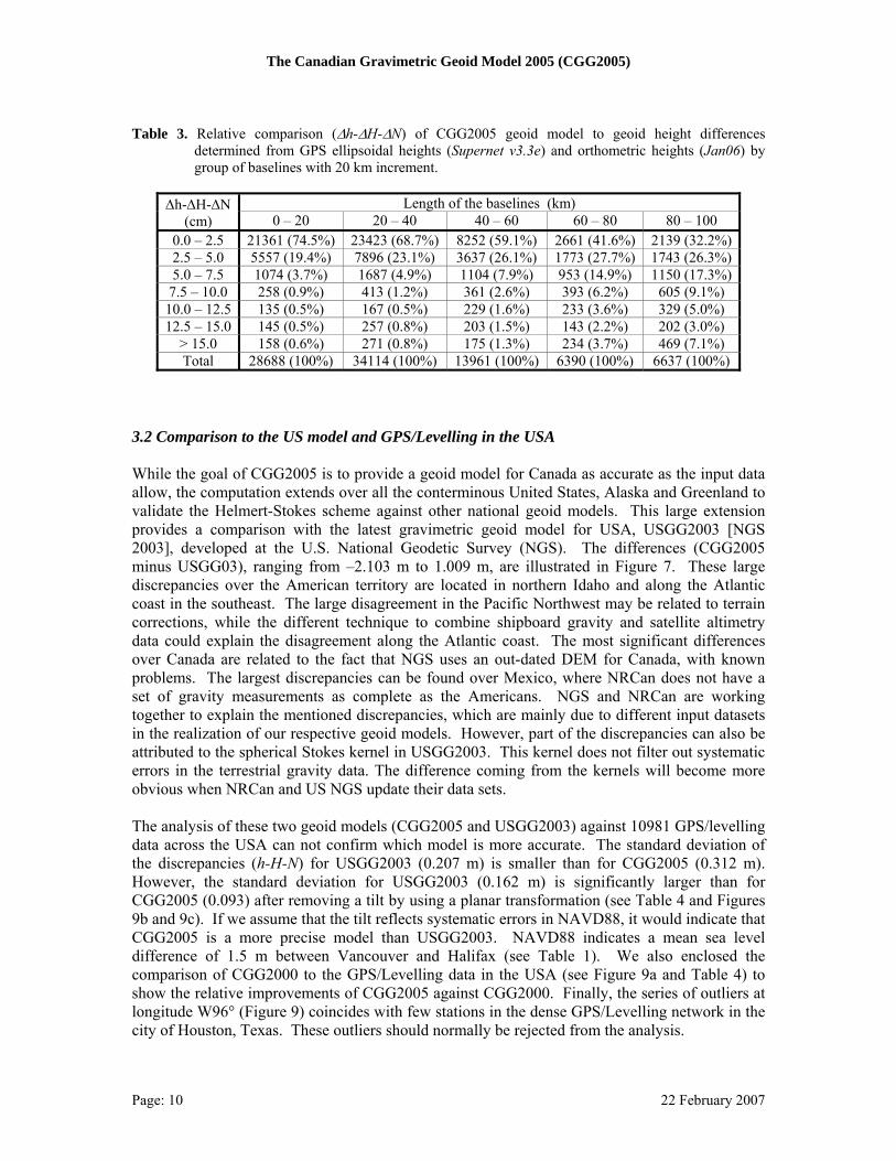
once in the 1970’s and formed large loops that do not close any better than at the decimetre level. One loop has a misclosure of 42 cm. Furthermore, most benchmarks in the Yukon Territory are five-foot rods installed in the permafrost making them quite unstable. The standard deviation of the discrepancies (hSN3.3e-HJan06-NCGG2005) for Newfoundland, PEI and Vancouver Island are 8.3 cm, 1.9 cm and 6.2 cm, respectively. However, the number of stations with GPS and levelling on PEI should be increased from the existing three stations, even though they cover the two ends of the island (175-km apart). The 1992 GPS campaign in Newfoundland should be re-observed to minimize errors from the ellipsoidal height component. The survey was never processed using precise orbits, as was the case all Canadian GPS surveys conducted prior to 1994. This may explain in part why the standard deviation of the discrepancies for Newfoundland does not improve significantly after fitting a planar transformation. The standard deviation is comparable to Canada’s main land even though the geographical area is much smaller. The levelling lines from the 1970’s, which were known to accumulate systematic error in the north-south direction due to the magnetic field, may also contribute to the problem. The discrepancies over Vancouver Island, which is approximately 450 km in length, may be attributed to a combination of systematic errors in the geoid model and levelling data. Finally, we enclose Figure 8c showing the discrepancies between CGG2005 and the geoid heights determined from the CGVD28 normal orthometric height and the Supernet v3.3e ellipsoidal heights. The figure shows well the existing distortion within CGVD28 that reaches the metre level. CGG2005 is also evaluated in a relative sense (∆h–∆H–∆N) for baselines less than 100 km. Most height applications are within that distance. Table 3 shows the number of baselines (and percentage) by increment of 20 km with precision within a certain range (e.g., 0.0 to 2.5 cm). The results indicate that 74.5% of the baselines less than 20 km in length have a precision better than 2.5 cm; however, this is not necessarily representative of the national precision. Most of those short baselines are concentrated around Great Slave Lake where the 1986 survey was conducted at ten-km spacing and in the Greater Vancouver Regional District where the Province of British Columbia conducted a high density GPS network on benchmarks. Overall, the “GPS on BM” projects in Canada have a spacing of approximately 30 km. The results for baselines longer than 20 km represent well the national average of the discrepancies, which include errors from geoid modeling, GPS heighting, geodetic levelling and stability of the benchmarks. All relative discrepancies are also shown in Figure 6 (in red). On the other hand, the black dots represent the mean discre-pancies for baselines regrouped by 10 km increment. The mean values increase with the distance from 2.0 cm to 6.0 cm indicating an accumulation of systematic errors coming from a combination of geoid modeling and geodetic level-ling. However, it is difficult to determine the source of these errors.

Figure 6: Relative discrepancies (∆hSN3.3d-∆HJan06-∆for baselines less than 100 km. The black dots are the meandiscrepancies for baselines grouped by 10-km increment.

NCGG2005)



Table 3. Relative comparison (∆h-∆H-∆N) of CGG2005 geoid model to geoid height differences

determined from GPS ellipsoidal heights (Supernet v3.3e) and orthometric heights (Jan06) by group of baselines with 20 km increment.

Length of the baselines (km) ∆h-∆H-∆N

(cm) 0 – 20 20 – 40 40 – 60 60 – 80 80 – 100 0.0 – 2.5 21361 (74.5%) 23423 (68.7%) 8252 (59.1%) 2661 (41.6%) 2139 (32.2%)2.5 – 5.0 5557 (19.4%) 7896 (23.1%) 3637 (26.1%) 1773 (27.7%) 1743 (26.3%)5.0 – 7.5 1074 (3.7%) 1687 (4.9%) 1104 (7.9%) 953 (14.9%) 1150 (17.3%)

7.5 – 10.0 258 (0.9%) 413 (1.2%) 361 (2.6%) 393 (6.2%) 605 (9.1%) 10.0 – 12.5 135 (0.5%) 167 (0.5%) 229 (1.6%) 233 (3.6%) 329 (5.0%) 12.5 – 15.0 145 (0.5%) 257 (0.8%) 203 (1.5%) 143 (2.2%) 202 (3.0%)

> 15.0 158 (0.6%) 271 (0.8%) 175 (1.3%) 234 (3.7%) 469 (7.1%) Total 28688 (100%) 34114 (100%) 13961 (100%) 6390 (100%) 6637 (100%)

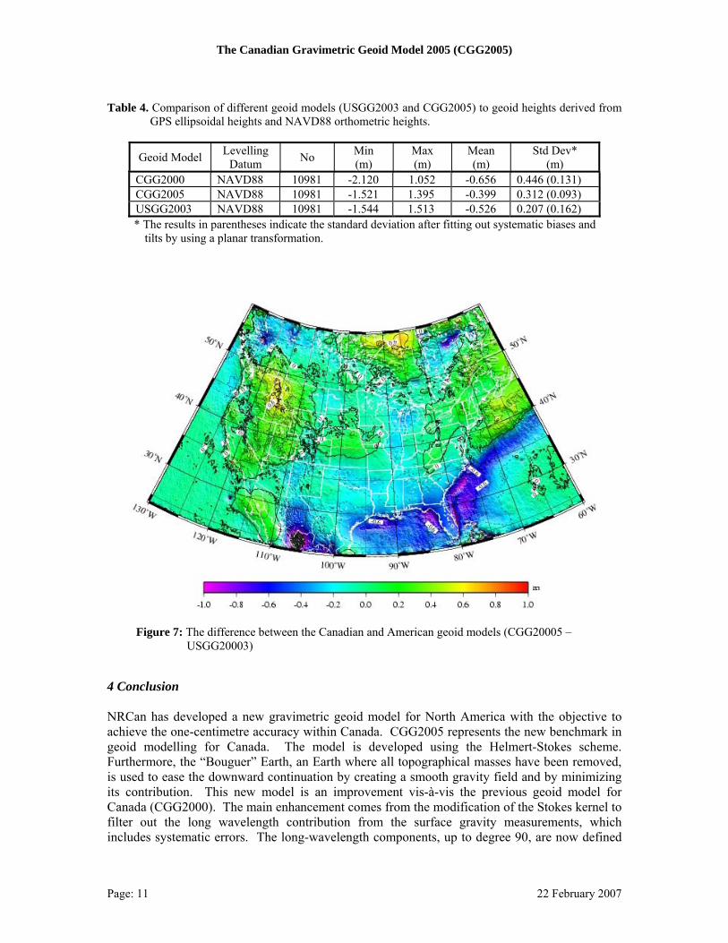
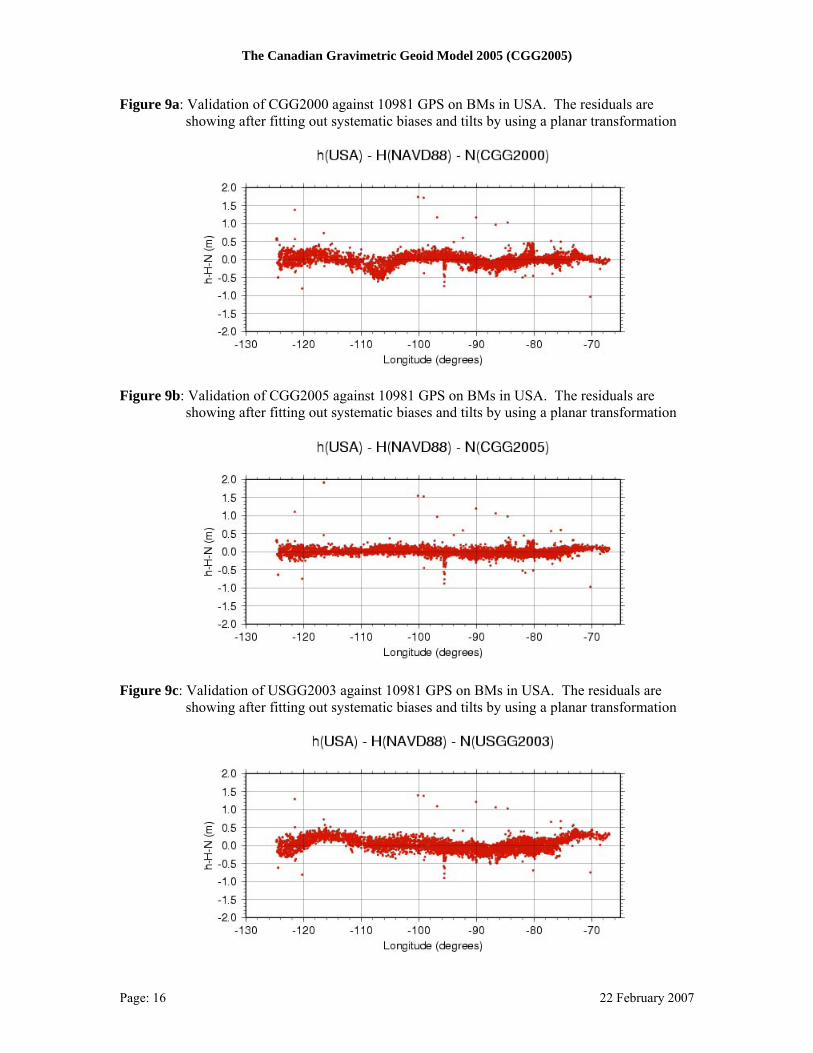
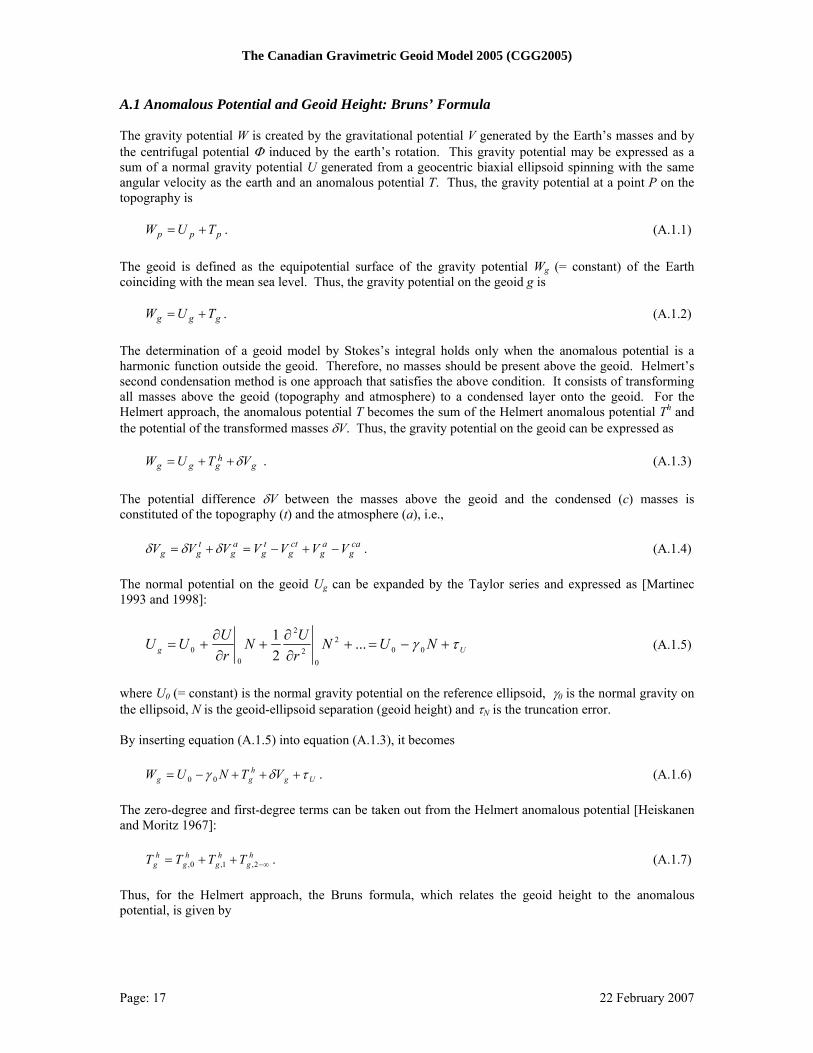
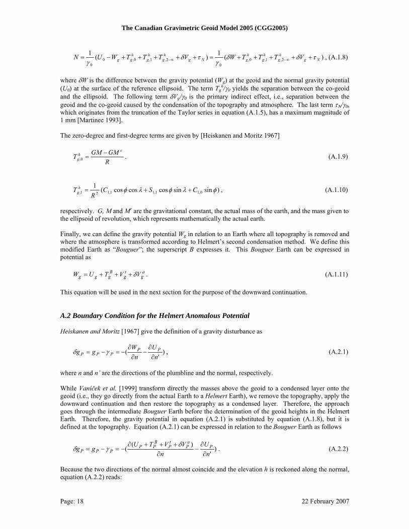
3.2 Comparison to the US model and GPS/Levelling in the USA While the goal of CGG2005 is to provide a geoid model for Canada as accurate as the input data allow, the computation extends over all the conterminous United States, Alaska and Greenland to validate the Helmert-Stokes scheme against other national geoid models. This large extension provides a comparison with the latest gravimetric geoid model for USA, USGG2003 [NGS 2003], developed at the U.S. National Geodetic Survey (NGS). The differences (CGG2005 minus USGG03), ranging from –2.103 m to 1.009 m, are illustrated in Figure 7. These large discrepancies over the American territory are located in northern Idaho and along the Atlantic coast in the southeast. The large disagreement in the Pacific Northwest may be related to terrain corrections, while the different technique to combine shipboard gravity and satellite altimetry data could explain the disagreement along the Atlantic coast. The most significant differences over Canada are related to the fact that NGS uses an out-dated DEM for Canada, with known problems. The largest discrepancies can be found over Mexico, where NRCan does not have a set of gravity measurements as complete as the Americans. NGS and NRCan are working together to explain the mentioned discrepancies, which are mainly due to different input datasets in the realization of our respective geoid models. However, part of the discrepancies can also be attributed to the spherical Stokes kernel in USGG2003. This kernel does not filter out systematic errors in the terrestrial gravity data. The difference coming from the kernels will become more obvious when NRCan and US NGS update their data sets. The analysis of these two geoid models (CGG2005 and USGG2003) against 10981 GPS/levelling data across the USA can not confirm which model is more accurate. The standard deviation of the discrepancies (h-H-N) for USGG2003 (0.207 m) is smaller than for CGG2005 (0.312 m). However, the standard deviation for USGG2003 (0.162 m) is significantly larger than for CGG2005 (0.093) after removing a tilt by using a planar transformation (see Table 4 and Figures 9b and 9c). If we assume that the tilt reflects systematic errors in NAVD88, it would indicate that CGG2005 is a more precise model than USGG2003. NAVD88 indicates a mean sea level difference of 1.5 m between Vancouver and Halifax (see Table 1). We also enclosed the comparison of CGG2000 to the GPS/Levelling data in the USA (see Figure 9a and Table 4) to show the relative improvements of CGG2005 against CGG2000. Finally, the series of outliers at longitude W96° (Figure 9) coincides with few stations in the dense GPS/Levelling network in the city of Houston, Texas. These outliers should normally be rejected from the analysis.



Table 4. Comparison of different geoid models (USGG2003 and CGG2005) to geoid heights derived from

GPS ellipsoidal heights and NAVD88 orthometric heights.

Geoid Model Levelling Datum No Min

(m) Max (m)

Mean (m)

Std Dev* (m)

CGG2000 NAVD88 10981 -2.120 1.052 -0.656 0.446 (0.131) CGG2005 NAVD88 10981 -1.521 1.395 -0.399 0.312 (0.093) USGG2003 NAVD88 10981 -1.544 1.513 -0.526 0.207 (0.162) * The results in parentheses indicate the standard deviation after fitting out systematic biases and

tilts by using a planar transformation.

Figure 7: The difference between the Canadian and American geoid models (CGG20005 – USGG20003)

4 Conclusion NRCan has developed a new gravimetric geoid model for North America with the objective to achieve the one-centimetre accuracy within Canada. CGG2005 represents the new benchmark in geoid modelling for Canada. The model is developed using the Helmert-Stokes scheme. Furthermore, the “Bouguer” Earth, an Earth where all topographical masses have been removed, is used to ease the downward continuation by creating a smooth gravity field and by minimizing its contribution. This new model is an improvement vis-à-vis the previous geoid model for Canada (CGG2000). The main enhancement comes from the modification of the Stokes kernel to filter out the long wavelength contribution from the surface gravity measurements, which includes systematic errors. The long-wavelength components, up to degree 90, are now defined



by GGM02C. This global gravity model includes early returns from the GRACE mission. CGG2005 has an estimated average internal accuracy of 2.6 cm, which is somewhat too optimistic since it does not consider systematic errors, omission errors and approximation. Comparison at 2269 GPS/levelling points distributed across Canada’s main land indicates a standard deviation of 13.0 cm, including errors from the GPS ellipsoidal heights, orthometric heights and stability of the benchmarks. The standard deviation becomes 7.2 cm after fitting a plane to the discrepancies to account for a possible 30-cm east-west systematic error in the levelling network. NRCan is already working on the next geoid model for Canada. This new model will again be based on the Helmert-Stokes scheme, but it will include more complete data sets. The Canadian gravity dataset will include the 2002 and 2003 airborne gravity surveys over Foxe Basin and Ungava Bay and a series of small gravity projects across the country. It will also include a more complete set of gravity measurements over the USA. The CDED 1:50k with a 0.75” horizontal resolution (~25 m), currently under production, will replace CDED1:250k across Canada. This will allow the computation of more accurate and homogeneous terrain corrections and mean Helmert gravity anomalies, which will be corrected for topographical density variation. The model also intends to make use of the GOCE data, which could deliver the geoid with accuracy at the centimetre level for wavelength components as short as 100 km. Finally, increased cooperation between NRCan, US NGS, INEGI (Mexico) and KMS (Denmark) could lead to the creation of a unified and accurate geoid model for North America. References Andersen, O.B. and P. Knudsen. 1998 Global marine gravity field from the ERS-1 and Geosat Geodetic

Mission Altimetry. J. Geophys. Res., Vol. 103, No. C4, p. 8129. Burša, M. 1995. Report of special commission SC3, Fundamental Constants. Presented at the 21st General

Assembly of the International Association of Geodesy, Boulder, CO, 2-14 July. Canon, J.B. 1929. Adjustment of the precise level net of Canada 1928. Publication No. 28, Geodetic Survey

Division, Natural Resources Canada, Ottawa, Canada. Craymer, M.R. and E. Lapelle. 1997. The GPS Supernet: An integration of GPS projects across Canada.

Report, Geodetic Survey Division, Natural Resources Canada, Ottawa. Cruz, J.Y. 1986. Ellipsoidal corrections to potential coefficients obtained from gravity anomaly data on the

ellipsoid. Report No. 371, Dept. of Geodetic Science and Surveying, The Ohio Sate University, Columbus, Ohio, USA.

Gruber, T., A. Bode, C. Reigber and P. Schwintzer. 1997. DPAF global Earth models based on ERS. Proceedings of 3. ERS Symposium, Florenz.

Haagmans, R., E. de Min and M. von Gelderen. 1993. Fast evaluation of convolution integrals on the sphere using 1D FFT, and a comparison with existing methods for Stokes’ integral. Manuscr geod 18:227-241.

Heiskanen, W.A. and H. Moritz. 1967 Physical Geodesy, Freeman. Huang, J., P. Vaníček, S.D. Pagiatakis and W. Brink. 2001. Effect of topographical density on the geoid in

the Canadian Rocky Mountains. Journal of Geodesy, 74: 805-815. Huang, J., G. Fotopoulous, M.K. Cheng, M. Véronneau and M.G. Sideris. 2006. On the estimation of the

regional geoid error in Canada. Proceedings of the International Association of Geodesy 2005. Huang, J. and M. Véronneau. 2005. Applications of downward-continuation in gravimetric geoid

modeling : case studies in Western Canada. J. Geod. 79: 135-145. Jekeli, C. 1981. The downward continuation to the Earth’s surface of truncated spherical and ellipsoidal

harmonic series of the gravity and height anomalies. Report No. 323, Dept. of Geodetic Science and Surveying, The Ohio Sate University, Columbus, Ohio, USA.



LeGrand, P., E.J.O. Schrama and J. Tournadre. 2003. An inverse estimate of the dynamic topography of the ocean. Geophys. Res. Lett., 30(2), 1062, doi:10.1029/2002GL014917.

Lemoine, F.G., S.C. Kenyon, J.K. Factor, R.G. Trimmer, N.K. Pavlis, D.S. Chinn, C.M. Cox, S.M. Klosko, S.B. Luthcke, M.H. Torrence, Y.M. Wang, R.G. Williamson, E.C. Pavlis, R.H. Rapp and T.R. Olson. 1998. The development of the joint NASA GSFC and the National Imagery and Mapping Agency (NIMA) Geopotential Model EGM96. National Aeronautics and Space Administration, Goddard Space Flight Center, Greenbelt, MD, USA.

Lemoine, J.M., R. Biancale, G. Balmino, J.C. Marty, B. Moynot, F. Barlier, Y. Boudon, P. Exertier, O. Laurain, P. Schwintzer, C. Reigber, A. Bode, K. Kang, F.H. Massman, H. Meixner, J.C. Raimondo and S. Zhu. 1999. The GRIM5 global geopotential model. Abstracts, International Union of Geodesy and Geophysics (IUGG) meeting, Birmingham, England.

Martinec, Z. 1993. Effect of lateral density variations of topographical masses in view of improving geoid model accuracy over Canada. Natural Resources Canada, Geodetic Survey Division, Ottawa. Report #93-002, 111 p.

Martinec, Z. 1998. Boundary-Value Problems for Gravimetric Determination of a Precise Geoid. Lecture Notes in Earth Sciences, 73, Springer.

National Geodetic Survey (NGS). 2003. Technical Information Page for USGG2003 and GEOID03. US NGS, NOAA, USA (http://www.ngs.noaa.gov/GEOID/GEOID03/tech.html).

Novák, P., P. Vaníček, Z. Martinec and M. Véronneau. 2001. Effects of the spherical terrain on gravity and the geoid. J Geod 75: 491-504.

Pagiatakis, S.D., D. Fraser, K. McEwen, A.K. Goodacre, and M. Véronneau. 2000. Topographic mass density and gravimetric geoid modelling. Boll Geof Teor Appl, V. 40, N. 3-4, pp. 189-194.

Pavlis, N.K., D.S. Chinn, C.M. Cox and F.G. Lemoine. 2000 Geopotential model improvement using POCM_4B dynamic ocean topography information: PGM2000A. Paper presented at the Joint TOPEX/Poseidon and Jason-1 Science Working Team Meeting, Miami, Florida, USA, 15-17 November.

Sandwell, D.T. and W.H.F. Smith. 1997. Marine gravity anomaly from Geosat and ERS 1 satellite altimetry. J. Geophys. Res., v. 102, No. B5, pp. 10039-10054.

Smith, D.A. and D. Roman. 2001. GEOID99 and G99SSS: 1-arc-minute geoid models for the United States. J Geod 75: 469-490.

Tapley, B., J. Ries, S. Bettadpur, D. Chambers, M. Cheng, F. Condi, B. Gunter, Z. Kang, P. Nagel, R. Pastor, T. Pekker, S. Poole and F. Wang. 2005. GGM02 – An improved Earth gravity field model from GRACE, J Geod, 79, 467-478.

Vaníček, P. and Z. Martinec. 1994. The Stokes-Helmert scheme for the evaluation of a precise geoid. Manusc Geod, 19, 119-128.

Vaníček, P., M. Najafi, Z. Martinec, L. harrie and L.E. Sjöberg. 1995. Hiher-degree reference field in the generalized Stokes-Helmert scheme for geoid computation. J. Geod., 70 176-182.

Vaníček, P., J. Huang and P. Novák. 1998. Atmosphere in the Stokes-Helmert solution of the geodetic boundary-value problem. Report, Geodetic Survey Division, Natural Resources Canada, Ottawa

Vaníček, P., J. Huang, P. Novák, S.D. Pagiatakis, M. Véronneau, Z. Martinec and W.E. Featherstone. 1999. Determination of the boundary values for the Stokes-Helmert problem. Journal of Geodesy, 73:180-192.

Véronneau, M. 1997. The GSD95 geoid model for Canada. Gravity, Geoid and Marine Geodesy, Proceedings of international symposium, Tokyo, Japan, 1996. Springer Vol. 117, pp. 573-580.

Véronneau, M., R. Duval and J. Huang. 2006. A vertical geoid model as a vertical datum for Canada. GEOMATICA, Vol. 60, No. 2, pp. 165-172.

Véronneau, M. 2001. The Canadian gravimetric geoid model of 2000 (CGG2000). Geodetic Survey Division, Natural Resources Canada, Ottawa, Canada.

Véronneau, M., A. Mainville and M.R. Craymer. 2001. The GPS Height Transformation (v2.0): An ellipsoidal-CGVD28 Height Transformation for use with GPS in Canada. Geodetic Survey Division, Natural Resources Canada, Ottawa, Canada.

Wieser, M. 1987. The global digital terrain model TUG’87. Internal report on set-up, origin, and characteristics. Institute of Mathematical Geodesy, Technical University, Graz.

Zilkoski, D.B. 1986. The new adjustment of the North American datum. ACSM Bulletin, April, pp. 35-36.



Zilkoski, D.B., J.H. Richards and G.M. Young. 1992. Results of the general adjustment of the North American vertical datum of 1988. American Congress on Surveying and Mapping, Surveying and Land Information Systems, 52(3), pp. 133-149.



Figure 8a: Validation of CGG2000 against 2274 GPS on BMs (Jan06) in Canada (Main land)

Figure 8b: Validation of CGG2005 against 2274 GPS on BMs (Jan06) in Canada (Main land)

Figure 8c: Validation of CGG2005 against 1962 GPS on BMs (CGVD28) in Canada



Figure 9a: Validation of CGG2000 against 10981 GPS on BMs in USA. The residuals are showing after fitting out systematic biases and tilts by using a planar transformation

Figure 9b: Validation of CGG2005 against 10981 GPS on BMs in USA. The residuals are

showing after fitting out systematic biases and tilts by using a planar transformation

Figure 9c: Validation of USGG2003 against 10981 GPS on BMs in USA. The residuals are

showing after fitting out systematic biases and tilts by using a planar transformation



A.1 Anomalous Potential and Geoid Height: Bruns’ Formula The gravity potential W is created by the gravitational potential V generated by the Earth’s masses and by the centrifugal potential Φ induced by the earth’s rotation. This gravity potential may be expressed as a sum of a normal gravity potential U generated from a geocentric biaxial ellipsoid spinning with the same angular velocity as the earth and an anomalous potential T. Thus, the gravity potential at a point P on the topography is

ppp TUW += . (A.1.1) The geoid is defined as the equipotential surface of the gravity potential Wg (= constant) of the Earth coinciding with the mean sea level. Thus, the gravity potential on the geoid g is

ggg TUW += . (A.1.2) The determination of a geoid model by Stokes’s integral holds only when the anomalous potential is a harmonic function outside the geoid. Therefore, no masses should be present above the geoid. Helmert’s second condensation method is one approach that satisfies the above condition. It consists of transforming all masses above the geoid (topography and atmosphere) to a condensed layer onto the geoid. For the Helmert approach, the anomalous potential T becomes the sum of the Helmert anomalous potential Th and the potential of the transformed masses δV. Thus, the gravity potential on the geoid can be expressed as

ghggg VTUW δ++= . (A.1.3)

The potential difference δV between the masses above the geoid and the condensed (c) masses is constituted of the topography (t) and the atmosphere (a), i.e.,

cag

ag

ctg

tg

ag

tgg VVVVVVV −+−=+= δδδ . (A.1.4)

The normal potential on the geoid Ug can be expanded by the Taylor series and expressed as [Martinec 1993 and 1998]:

Ug NUNrUN

rUUU τγ +−=+

∂∂

+∂∂

+= 002

02

2

00 ...

21

(A.1.5)

where U0 (= constant) is the normal gravity potential on the reference ellipsoid, γ0 is the normal gravity on the ellipsoid, N is the geoid-ellipsoid separation (geoid height) and τN is the truncation error. By inserting equation (A.1.5) into equation (A.1.3), it becomes

Ugh

gg VTNUW τδγ +++−= 00 . (A.1.6) The zero-degree and first-degree terms can be taken out from the Helmert anomalous potential [Heiskanen and Moritz 1967]:

hg

hg

hg

hg TTTT ∞−++= 2,1,0, . (A.1.7)

Thus, for the Helmert approach, the Bruns formula, which relates the geoid height to the anomalous potential, is given by



)(1)(12,1,0,

02,1,0,0

0Ng

hg

hg

hgNg

hg

hg

hgg VTTTWVTTTWUN τδδ

γτδ

γ+++++=+++++−= ∞−∞− , (A.1.8)

where δW is the difference between the gravity potential (Wg) at the geoid and the normal gravity potential (U0) at the surface of the reference ellipsoid. The term Tg

h/γ0 yields the separation between the co-geoid and the ellipsoid. The following term δVg/γ0 is the primary indirect effect, i.e., separation between the geoid and the co-geoid caused by the condensation of the topography and atmosphere. The last term τΝ/γ0, which originates from the truncation of the Taylor series in equation (A.1.5), has a maximum magnitude of 1 mm [Martinec 1993]. The zero-degree and first-degree terms are given by [Heiskanen and Moritz 1967]

RGMGMT

eh

g−

=0, . (A.1.9)

)sinsincoscoscos(10,11,11,121, φλφλφ CSC

RT h

g ++= , (A.1.10)

respectively. G, M and Me are the gravitational constant, the actual mass of the earth, and the mass given to the ellipsoid of revolution, which represents mathematically the actual earth. Finally, we can define the gravity potential Wg in relation to an Earth where all topography is removed and where the atmosphere is transformed according to Helmert’s second condensation method. We define this modified Earth as “Bouguer”; the superscript B expresses it. This Bouguer Earth can be expressed in potential as

ag

tg

Bggg VVTUW δ+++= . (A.1.11)

This equation will be used in the next section for the purpose of the downward continuation. A.2 Boundary Condition for the Helmert Anomalous Potential Heiskanen and Moritz [1967] give the definition of a gravity disturbance as

)'

(n

Un

Wgg PP

PPP ∂∂

−∂∂

−=−= γδ , (A.2.1)

where n and n’ are the directions of the plumbline and the normal, respectively. While Vaníček et al. [1999] transform directly the masses above the geoid to a condensed layer onto the geoid (i.e., they go directly from the actual Earth to a Helmert Earth), we remove the topography, apply the downward continuation and then restore the topography as a condensed layer. Therefore, the approach goes through the intermediate Bouguer Earth before the determination of the geoid heights in the Helmert Earth. Therefore, the gravity potential in equation (A.2.1) is substituted by equation (A.1.8), but it is defined at the topography. Equation (A.2.1) can be expressed in relation to the Bouguer Earth as follows

)'

)((

nU

nVVTU

gg Pa

PtP

BPP

PPP ∂∂

−∂

+++∂−=−=

δγδ . (A.2.2)

Because the two directions of the normal almost coincide and the elevation h is reckoned along the normal, equation (A.2.2) reads:



n

aP

tP

BP

PPP hVVT

gg εδ

γδ −∂

++∂−=−= )

)(( , (A.2.3)

where εn is the correction for the substitution of the direction of the normal. This correction can be neglected because it reaches only a few µGal [Cruz 1986]. Normal gravity γP can be expanded by means of γ and its derivatives in a Taylor series at point 0 on the ellipsoid, i.e.,

γγ τγγγγγγ +∂∂

+−=−+∂∂

++∂∂

+= Nh

DNHh

NHhP

00

2

02

2

00 ...)(

21)( , (A.2.4)

where Dγ is the normal free-air reduction (normal gradient of gravity time height) to the second order term between the topography surface and geoid. It is defined as follows [Heiskanen and Moritz 1967]

22020 3

)sin21(2

Ha

Hfmfa

Dγ

φγ

γ −−++= . (A.2.5)

Inserting equation (A.2.4) into equation (A.2.3), it becomes

n

P

a

P

t

P

B

PP hV

hV

hTN

hDgg εδτγγδ γγ −

∂∂

−∂∂

−∂∂

−=+∂∂

−+−=0

0 , (A.2.6)

and it can also be expressed as:

nP

a

P

t

FAP

B

hV

hVN

hg

hT ετδγ

γ ++∂

∂+

∂∂

+∂∂

−∆=∂∂

−0

. (A.2.7)

Equation (A.2.7) corresponds to a gravity disturbance for the Bouguer Earth. The free-air anomaly is expressed by ∆gFA. Because the disturbance is defined at the topography, it must be downward continued to the geoid. Taking spherical approximation of the second term, eq. (A.2.7) can be expressed on the geoid as

γδ τεδεεεδγ++++++

∂∂

+∂∂

+∂∂

−∆=∂∂

− na

ht

hB

hgP

a

P

t

FAg

BVVTD

rV

rVN

hg

rT

B )()()(0

,

(A.2.8)

where the ellipsoidal correction term εh(TB) is given by [Jekeli 1981; Cruz 1986]

)(cossin1cossin 22 Bh

BB

BBBBT

rTe

rTT

re

rT

hT εγξφφ

φφφ −

∂∂

−=+∂∂

−=∂∂

−∂∂

−≅∂∂

− , (A.2.9)

and Dδg

B is the downward continuation of gravity disturbances for the Bouguer Earth. It is given by [Huang and al. 2005]



P

B

g

B

g rT

rTD B

∂∂

+∂∂

−=δ . (A.2.10)

Substituting N by equation (A.1.7) and adding the condensed topographical effect on each side of equation (A.2.8), it now reads

γδ τεεδτδδγ

γ++++

∂∂

+∂∂

−∂∂

+∆=+++∂∂

+∂∂

− )()(1

00

TDrV

rV

rVgVTW

hrT

hngP

a

g

ct

P

t

FAUgh

gg

h

B .

(A.2.11) The derivative of the normal gravity along the normal can be expressed as (Jekeli, 1981 and Cruz, 1986)

)(2)2sin3(21 22

00χεχχφχχγ

γ γ−−=−+−≅∂∂

rre

rh, (A.2.12)

where χ can be substituted by δW, Tg

h, δVg and τn. Substituting the above equation in equation (A.2.11), it becomes

Ε+++++∂

∂+

∂∂

−∂∂

+∆≅−∂∂

− )(22Ngg

P

a

g

ct

P

t

FAh

gg

hVW

rD

rV

rV

rVgT

rrT

B τδδδδ (A.2.13)

or

Ε+++++∂

∂+

∂∂

−∂∂

+∆≅∆ )(2Ngg

P

a

g

ct

P

t

FAhg VW

rD

rV

rV

rVgg B τδδδ

δ , (A.2.14)

where

γγγγ τετεδεεε +++++=Ε nNgPh WTT )()()()( . (A.2.15) Equation (A.2.13) defines a Helmert gravity anomaly on the geoid. A.3 Stokes’s Integral In appendix A.1, we demonstrated that geoid heights could be determined from the Bruns formula. Thus, Equation (A.1.8) can also be expressed as [Heiskanen and Moritz 1967]

N

NNdSgRTR

MGWN PIEhg

hg

τεψπγγγ

δγδ

+++Ω∆+++= ∫Ω

100

1,

00

)(4

, (A.3.1)

where the fourth term on the right hand side is the Stokes integral, NPIE is the primary indirect effect, ε1 is the ellipsoid correction for the spherical Stokes kernel S(ψ) and Nτ is the truncation error. The primary indirect effect contains the contribution from the topography and atmosphere. Because Helmert gravity anomalies determined from observed gravity and heights contain biases, we remove the long wavelength components of the gravity measurements by subtracting the first l degrees from the Stokes kernel. The long wavelengths up to degree l are added back from a global geopotential model Nl

h in a Helmert Earth. Equation (A.3.1) becomes



NNNdSgRN

TR

MGWN lPIE

lhg

hTl

hg

τεψπγγγ

δγδ

+++Ω∆++++= ∫Ω

− 10

,2

0

1,

00

)(4

, (A.3.2)

where ε1

l is the ellipsoidal correction above degree l. The superscript T represents the true long wavelength components of the geoid model. The modified Stokes kernel Sl(ψ) can be expressed as [Huang and Véronneau 2005]

∑= −

+=

m

nn

l PnnS

2

)(cos112)( ψψ . (A.3.3)

where m coincides with the sampling interval of the terrestrial gravity data. Because we do not have gravity measurements available over the whole world, we split the Stokes integral into two areas: 1) an area σ where we have surface gravity measurements and 2) an area Ω−σ where we might not have any observed gravity. Ω corresponds to the integration over the whole Earth. Equation (A.3.2) now reads

NNNdSgRdSgRN

TR

MGWN lPIE

lhg

lhg

hTl

hg

τ

σσ

εψπγ

ψπγγγ

δγδ

+++Ω∆+Ω∆++++= ∫∫−Ω

− 100

,2

0

1,

00

)(4

)(4

(A.3.4)

Naturally, for evaluating a geoid height, one requires gravity measurements globally. Thus, a global geopotential model can approximate the actual gravity measurements outside area σ. A.4 Spherical Harmonic Gravity Model The gravitational potential is given by

( ) )(sinsincos102∑∑==

+⎟⎠⎞

⎜⎝⎛−=

n

mnmnmnm

N

n

n

PmSmCra

rGMV φλλ . (A.4.1)

Spherical harmonic expansion of the normal gravitational potential is

( ) )(sin1 002

* φnn

N

n

neePJ

ra

rGMU ∑

=⎟⎟⎠

⎞⎜⎜⎝

⎛−= . (A.4.2)

Therefore, using the disturbing potential and Bruns’ formula, one derives

∑∑== ⎟⎟

⎟

⎠

⎞

⎜⎜⎜

⎝

⎛+⎟

⎟⎠

⎞⎜⎜⎝

⎛−⎟⎟

⎠

⎞⎜⎜⎝

⎛+=

n

mnmnmn

nee

nm

L

n

n

eeeL PmSmJ

aa

GMGMC

ra

rGM

rMGN

0200)(sinsincos)( φλλ

γγδ (A.4.3)

and

∑∑== ⎟⎟

⎟

⎠

⎞

⎜⎜⎜

⎝

⎛+⎟

⎟⎠

⎞⎜⎜⎝

⎛−−⎟⎟

⎠

⎞⎜⎜⎝

⎛+=∆

n

mnmnmn

nee

nm

L

n

n

eeeL PmSmJ

aa

GMGMCn

ra

rGM

rMGg

0222 )(sinsincos)()1( φλλδ

(A.4.4)



where ΝL and ∆gL are the geoid height and free-air anomaly up to degree and order L, respectively. The difference between the mass of the equipotential ellipsoid of revolution (Me) and the mass of and the actual earth (M) is taken into consideration by the first term. Because the boundary-value problem is solved using Helmert second condensation method, the spherical harmonic expansion must also be transformed to the Helmert Earth [Vaníček et al., 1995]. Tihs transformation can be expressed as Nh

L = T(NL) and ∆ghL = T(∆gL).

The geoid height Nh

L, which is determined from the spherical harmonic expansion, can also be evaluated from the Stokes integral:

200

0 )()(42

εψφπγγ

δ+Ω∆+=+= ∫

Ω−

dSgRr

MGNNN hL

e

hhhLL

. (A.4.5)

The ellipsoidal correction ε2 is a correction for the spherical Stokes kernel. As previously, the geoid height Nh

L can be determined from the degree-banded Stokes kernel Sl(ψ) of degree l and the integral split into the same two regions

llhL

lhL

hhh dSgRdSgRNNNlL 2

00)(

)(4)(

)(420εψ

φπγψ

φπγσσ

+Ω∆+Ω∆++= ∫∫−Ω

−. (A.4.6)

The degree L (>= 360) is significantly higher than the degree l (<= 90). We replace in equation (A.3.4) the actual long wavelength components of the geoid heights (Nh

2-l) and the unknown gravity anomalies (∆ghg)

by their spherical harmonic values as an approximation. Equation (A.3.4) reads

++++≅ −h

l

hg N

TR

MGWN 20

1,

00 γγδ

γδ

NLNNdSgRdSgR l

PIElhlh

g τσσ

εψπγ

ψπγ

+++Ω∆+Ω∆ ∫∫−Ω

100

)(4

)(4

(A.4.7)

The NlPIE term is the primary indirect effects on the first l degrees. It allows the transformation of the long

wavelengths from the actual Earth to the Helmert Earth. Finally, by subtracting equation (A.4.6) from equation (A.4.7), it becomes

ULLNNdSggRN

TR

MGWN llPIE

lhhg

hh

gτ

σ

εεψπγγγ

δγδ

+−++Ω∆−∆++++≅ ∫ 2100

1,

00)()(

4. (A.4.8)

ε1

l-ε2l represents the ellipsoidal correction due to the residual gravity anomalies above degree and order l.

A.5 Mean Helmert anomalies For the determination of the geoid model for Canada, the Helmert gravity anomalies used into the Stokes integral are actually a mean over a geographical cell. Therefore, the mean Helmert anomaly is defined as

∫Ω

ΩΩ∆=∆ dgA

g hg

hg )(1 , (A.5.1)

where A is the area of the cell.



Because of the limited number of gravity measurements, the mean gravity anomalies are estimated from surrounding observations, which may not lie necessarily within the cell. The proposed approach is based on two concepts: 1) the refined Bouguer anomalies offer a relatively smooth gravity field for interpolation and averaging; and 2) least-squares collocation is an efficient method for gravity prediction. This is the same approach as for GSD95 [Véronneau 1997] and CGG2000 [Véronneau 2001]. The refined Bouguer anomaly is defined as [Heiskanen and Moritz 1967]

tFA

rB AHGgg0

2 ψρπ +−∆=∆ , (A.5.2) where 2πGρH is the Bouguer plate and At is the terrain correction within a radius ψ0 = 50 km. The mean refined Bouguer anomaly can be determined as

)(1,1

1

rBmj

n

ii

rBgC

ng =

=

∆=∆ ∑ , (A.5.3)

where C is the least-squares collocation operator, n (= 9) is the number of sub-areas within area A and m (=20) is the number of observations (5 nearest observations from each quadrant). From equation (A.2.14), we can write the removal of the topography, the restoration of condensed topography and the atmospheric correction as

STCBAAABr

V tp

ttttp

P

t+=+++=

∂∂

210 ψψψ , (A.5.4)

CTEBAABAAABr

V ctg

ctctctg

ctctctctg

g

ct+≅++≅+++=

∂∂

21210 ψψψψψ , (A.5.5)

and

a

P

aA

rV δδ

=∂

∂ , (A.5.6)

respectively. Bp

t and Bgct are the attraction of the Bouguer shell and condensed Bouguer shell, respectively.

They are given by [Martinec 1998]

)3

1()(

42

2

2

2

RH

RH

HRRHGBt

p +++

−= ρπ (A.5.7)

2

2

)(4

HRRGB ct

g+

−= σπ , (A.5.8)

where σ is the condensed topographical density

)3

1( 2

2

RH

RHH ++= ρσ . (A.5.9)

The subscripts ψ0, ψ1 and ψ2 to the spherical terrain correction (STC) and condensed terrain effect (CTE) represent integration areas ranging from 0 to 50 km, 50 km to 3.0 degrees and outside the three-degree cap, respectively. The three zones are evaluated by numerical integration. However, the contribution of the



condensed topography on the geoid in the innermost zone Aψ0ct is small. Its contribution to the geoid model

reaches 4 mm. Whereas the difference between the attractions of the Bouguer shell at the topography and the condensed shell at the geoid can contribute up to 5 cm in the Canadian Rocky Mountains. Therefore, by inserting equations (A.5.3), (A.5.4), (A.5.5) and (A.5.6) into equation (A.2.14), it yields

Ε++++++−−++−++∆≅∆ )(222121 Ngg

actctttctg

tpDEMrB

hg VW

rDAAAAABBHGgg rB τδδδρπ δψψψψ .

(A.5.10) Equation (A.5.10) describes a mean Helmert anomaly on the geoid. A.6 Primary and secondary Indirect Effect In CGG2000, the formulation for the primary indirect terrain effect (PITE) was given by Martinec [1993; 1998]. However, in CGG2005, PITE is determined following a different formulation, which includes a near zone (δNI,NZ) and a far zone (δNI,FZ). The near zone contribution corresponds to the total topographical mass within a spherical radius ψ0 from the computational point. The near-zone contribution is computed by the following formula:

[ ] ΩΩ−Ω+Ω

−Ω

= ∫Ω

+=

+= drRKrRKGVV

N HRRr

HRRr

ccapcapNZI

'0

''

', |)',,(~)(|)',,(~)'()()(

ψρψργγγ

δ

[ ] '),,()()()'()'( 21

'0

ΩΩ−Ω− −

Ω∫ dRRRLHHG ψτρτρ

γ (A.6.1)

where

HR

Rr

cap rRLR

rrRGV

+

==⎥⎥⎦

⎤

⎢⎢⎣

⎡⎟⎟⎠

⎞⎜⎜⎝

⎛+−

−−Ω=Ω

'0

22 0

)',,(3'

6cos'

6)2cos3(

)(2)(

ψ

ψ

ψψψρπ

( ) ([ ]) HR

RrrRLrRRG

+

==+−−Ω−

'032 0)',,('_coslncos(cos)(

ψ

ψψψψψρπ (A.6.2)

2sin)()(4)( 0ψ

τρπ HGRVccap Ω=Ω (A.6.3)

CrrLrrrrrLrrrrK ++−−++= )',,(cos'ln)1cos3(2

)',,()cos3'(21)',,(~ 2

2ψψψψψψ (A.6.4)

21

22 )'cos'2()',,( rrrrrrL +−= ψψ (A.6.5)

⎟⎟⎠

⎞⎜⎜⎝

⎛++= 2

2

31)(

RH

RHHHτ (A.6.6)



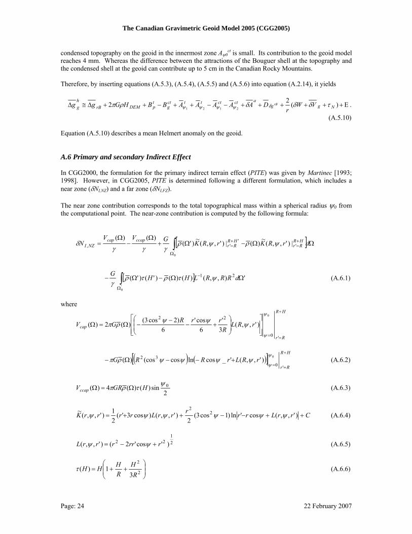
The magnitude of the near zone contribution is shown in Table A.6.1 for a test region in the Canadian Rockies where DEMs with different horizontal resolution (2’, 1’ and 30”) are analyzed using a 1 arc-degree integration cap size. The resolution of the DEM between 30” and 2’ does not play a major role in PITE where the RMS difference is only 2 mm for the test region. Table A.6.1. Contribution of the primary indirect terrain effect in the near-zone (ψ0 = 1°) for DEMs with

different horizontal resolutions within the Canadian Rocky Mountains (W119°-W120°; N51°-N52°).

DEM

Resolution Min. (m)

Max. (m)

Mean (m)

Std.Dev. (m)

RMS (m)

2’by2’ -0.251 -0.017 -0.103 0.046 0.113 1’by1’ -0.275 -0.014 -0.104 0.047 0.114 0.5’by0.5’ -0.279 -0.014 -0.105 0.047 0.115

While the formulation for the far-zone contribution can be expressed as:

[ ] '),,()'()'('|)',,(~)'( 21

''

'',

'0

'0

ΩΩ−ΩΩ= −

Ω−ΩΩ−Ω

+= ∫∫ dRRRLHGdrRKGN HR

RrFZI ψτργ

ψργ

δ (A.6.7)

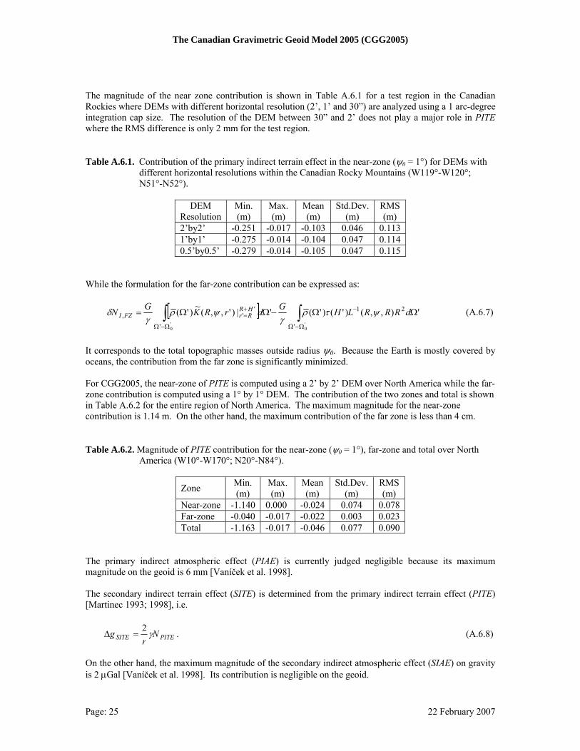
It corresponds to the total topographic masses outside radius ψ0. Because the Earth is mostly covered by oceans, the contribution from the far zone is significantly minimized. For CGG2005, the near-zone of PITE is computed using a 2’ by 2’ DEM over North America while the far-zone contribution is computed using a 1° by 1° DEM. The contribution of the two zones and total is shown in Table A.6.2 for the entire region of North America. The maximum magnitude for the near-zone contribution is 1.14 m. On the other hand, the maximum contribution of the far zone is less than 4 cm. Table A.6.2. Magnitude of PITE contribution for the near-zone (ψ0 = 1°), far-zone and total over North

America (W10°-W170°; N20°-N84°).

Zone Min. (m)

Max. (m)

Mean (m)

Std.Dev. (m)

RMS (m)

Near-zone -1.140 0.000 -0.024 0.074 0.078 Far-zone -0.040 -0.017 -0.022 0.003 0.023 Total -1.163 -0.017 -0.046 0.077 0.090

The primary indirect atmospheric effect (PIAE) is currently judged negligible because its maximum magnitude on the geoid is 6 mm [Vaníček et al. 1998]. The secondary indirect terrain effect (SITE) is determined from the primary indirect terrain effect (PITE) [Martinec 1993; 1998], i.e.

PITESITE Nr

g γ2=∆ . (A.6.8)

On the other hand, the maximum magnitude of the secondary indirect atmospheric effect (SIAE) on gravity is 2 µGal [Vaníček et al. 1998]. Its contribution is negligible on the geoid.


Documents

The Canadian Gravimetric Geoid Model 2005 … Canadian Gravimetric Geoid Model 2005 (CGG2005) Marc Véronneau and Jianliang Huang Geodetic Survey Division, Natural Resources Canada,