The Blowup Formula for Higher Rank Donaldson

Invariants

by

Lucas Howard Culler

Submitted to the Department of Mathematicsin partial fulfillment of the requirements for the degree of

Doctor of Philosophy

at the

MASSACHUSETTS INSTITUTE OF TECHNOLOGY

June 2014

@Lucas Culler 2014. All rights reserved.

Signature redacted

NAASSAr'HUSETTS INSiiESTECHNOLOGY

JUN 1 201

LBRARIES

Author.......Department of Mathematics

May 1, 2014

<Signature redactedCertified by.

Tomasz MrowkaSinger Professor of Mathematics

Thesis Supervisor

Signature redactedAccepted by... .......................

Alexei BorodinChairman, Department Committee on Graduate Theses

2

The Blowup Formula for Higher Rank Donaldson Invariantsby

Lucas Howard Culler

Submitted to the Department of Mathematicson May 1, 2014, in partial fulfillment of the

requirements for the degree ofDoctor of Philosophy

Abstract

In this thesis, I study the relationship between the higher rank Donaldson invariants

of a smooth 4-manifold X and the invariants of its blowup X#CP2 . This relationship

can be expressed in terms of a formal power series in several variables, called the blowup

function. I compute the restriction of the blowup function to one of its variables, by solving a

special system of ordinary differential equations. I also compute the SU(3) blowup function

completely, and show that it is a theta function on a family of genus 2 hyperelliptic Jacobians.

Finally, I give a formal argument to explain the appearance of Abelian varieties and theta

functions in four dimensional topological field theories.

Thesis Supervisor: Tomasz Mrowka

Title: Singer Professor of Mathematics

The author was partially supported by NSF grant DMS-0943787.

3

4

Acknowledgments

First and foremost I would like to thank my advisor Tom Mrowka, for introducing meto gauge theory, providing me with an excellent thesis problem, and patiently listening to

me as I blundered my way through it. I would also like to thank the other two members

of my thesis committee, Peter Kronheimer and Paul Seidel, for their useful input and fororganizing stimulating courses and seminars.

I have had an uncountable number of interesting and stimulating mathematical conver-sations with my peers during the last few years. My discussions on gauge theory and Floerhomology with Josh Batson, Aliakbar Daemi, and Jon Bloom were particularly useful and

relevant to my thesis, as were dicussions with Sam Raskin and Matt Wolfe on algebraic

geometry. Many other friends have influenced my view of mathematics over the years, es-

pecially Raju Krishnamoorthy, Philip Engel, Ailsa Keating, Tiankai Liu, Aaron Silberstein,Dustin Clausen, and Peter Smillie. I should also point out that this thesis would have been

impossible without Dan Gardner, who initiated me in the mysteries of theta functions as anundergraduate.

I owe special gratitude to Glenn Stevens and the PROMYS program, which introduced

me to mathematics as a high school student. This wonderful program taught me that therewas truth in the world, and that I could find it myself if I only knew how to look.

Finally, I would like to thank my parents, who have always supported me in every way,and without whom I would be nothing at all.

5

6

Contents

1 Introduction 9

2 Higher Rank Invariants 13

2.1 ASD Connections ................................ . 13

2.1.1 The Configuration Space ......................... 13

2.1.2 The Moduli Space . . . . . . . . . . . . . . . . . . . . . . . . . . . . 15

2.1.3 Index Theory . . . . . . . . . . . . . . . . . . . . . . . . . . . . . . . 172.1.4 Reducibles . . . . . . . . . . . . . . . . . . . . . . . . . . . . . . . . . 192.1.5 Perturbations . . . . . . . . . . . . . . . . . . . . . . . . . . . . . . . 20

2.1.6 Orientations . . . . . . . . . . . . . . . . . . . . . . . . . . . . . . . . 22

2.2 Donaldson Invariants . . . . . . . . . . . . . . . . . . . . . . . . . . . . . . . 22

2.2.1 Cohomology Classes . . . . . . . . . . . . . . . . . . . . . . . . . . . 23

2.2.2 Invariants . . . . . . . . . . . . . . . . . . . . . . . . . . . . . . . . . 25

2.3 Cylindrical Ends and Gluing . . . . . . . . . . . . . . . . . . . . . . . . . . . 292.3.1 Cylindrical Ends . . . . . . . . . . . . . . . . . . . . . . . . . . . . . 292.3.2 The Equivariant Universal Bundle . . . . . . . . . . . . . . . . . . . . 31

2.3.3 Index Theory . . . . . . . . . . . . . . . . . . . . . . . . . . . . . . . 322.3.4 The Gluing Theorem . . . . . . . . . . . . . . . . . . . . . . . . . . . 34

3 Higher Rank Blowup Formulas 37

3.1 Solutions Near a Negative Sphere . . . . . . . . . . . . . . . . . . . . . . . . 37

3.1.1 Regularity . . . . . . . . . . . . . . . . . . . . . . . . . . . . . . . . . 373.1.2 Completely Reducible Connections . . . . . . . . . . . . . . . . . . . 40

3.2 The Blowup Formula . . . . . . . . . . . . . . . . . . . . . . . . . . . . . . . 44

3.2.1 Initial Conditions . . . . . . . . . . . . . . . . . . . . . . . . . . . . . 443.2.2 A Simple Relation . . . . . . . . . . . . . . . . . . . . . . . . . . . . 463.2.3 Partial Blowup Functions . . . . . . . . . . . . . . . . . . . . . . . . 49

3.2.4 Full Blowup Functions . . . . . . . . . . . . . . . . . . . . . . . . . . 51

3.3 The Case N=3 . . . . . . . . . . . . . . . . . . . . . . . . . . . . . . . . . . 543.3.1 Theta Functions on a Genus 2 Jacobian . . . . . . . . . . . . . . . . 54

3.3.2 The Blowup Function . . . . . . . . . . . . . . . . . . . . . . . . . . . 57

4 The Formal Picture 59

4.1 A xiom s . . . . . . . . . . . . . . . . . . . . . . . . . . . . . . . . . . . . . . . 594.2 The Formal Blowup Formula . . . . . . . . . . . . . . . . . . . . . . . . . . . 60

7

4.3 The Blowup Algebra . . . . . . . . . . . . . . . . . . . . . . . . . . . . . . . 634.4 Geometry of the Blowup Algebra . . . . . . . . . . . . . . . . . . . . . . . . 654.5 Analytic Continuation . . . . . . . . . . . . . . . . . . . . . . . . . . . . . . 674.6 Periods and Theta Functions . . . . . . . . . . . . . . . . . . . . . . . . . . . 70

8

Chapter 1

Introduction

Donaldson's invariants of smooth 4-manifolds were originally defined using moduli spaces

of anti-self dual connections on principal bundles with structure group SU(2) or SO(3) =

PU(2). These invariants and their corresponding generating functions have many interesting

structural features which have been described in a mathematically rigorous way. For instance,

a paper of Fintushel and Stern [7] shows that the invariants of a 4-manifold X and its blowup

X = X#Cp2 are related in a predictable way, and that the relationship can be expressed in

terms of a theta function on the elliptic curve

y2 = 3 +a2+Xy2 =x+ax2+x

over the ring Q[a]. More generally, the structure theorem of Kronheimer-Mrowka expresses

the Donaldson invariants of a 4-manifold of simple type in terms of exponential functions

(theta functions on a degenerate genus 1 curve), and there is a conjectural structure theorem

for 4-manifolds not of simple type, which expresses the invariants of such a manifold in terms

of Jacobi elliptic functions.

It is natural to ask if Donaldson invariants can be defined for higher rank bundles, and if so,

whether or not these structural features have some natural generalization. Indeed, physicists

have achieved results in this direction (see for example [3] and [12]), which indicate that the

blow-up formula and structure theorem for SU(N) invariants can be expressed in terms of

function theory on the hyperelliptic curve

EN: y= (N + a2N-2 + + aN-1X + aN)2 (.)

over the ringA = H*(BPU(N); Q) = Q[a2 , . . , aN].

In particular it is shown in [3] that the blow-up function is a theta function on the Ja-

cobian of this curve, generalizing the result of Fintushel and Stern. Unfortunately, their

derivation relies on the use of quantum field theory techniques, which do not appear to be

mathematically rigorous.

One route to overcoming these difficulties, pursued by Nakajima and Yoshioka in [14],

is through Nekrasov's partition function. Using the localization formula in equivariant co-

homology, they rigorously define certain integrals which are analogous to the Donaldson

9

invariants of the plane blown up at a single point. They compute these integrals using tech-niques of algebraic geometry, and thereby arrive at a blow-up formula which agrees with theone from the physics literature.

It is not clear, however, what either of the methods above has to do with moduli spacesof instantons on general 4-manifolds. In this paper we take a more direct route. In [8],Peter Kronheimer has given a rigorous definition of PU(N) invariants for general N. Usinghis definition we directly attempt to compute the blowup function, using the method ofFintushel and Stern. For small values of N we compute the blowup function recursively, andfor N = 3 we explicitly identify it with a theta function on the Jacobian of the curve E3-For general N we can partially compute the blowup function. More precisely, we restrict theblowup function to one of its variables and characterize the resulting single variable functionby a system of ordinary differential equations. After a change of variables, this system ofequations reduces to the Toda chain, an integrable system well-known to physicists, whoserelation with the blowup formula was predicted in [12].

Theta functions also arise in Seiberg-Witten theory, where the analogous blowup formula[9] is encoded by an infinite Laurent series over the formal power series ring Z[[U]]:

O(T) = (-1)"Un TnEZ

This formal sum can be viewed as a theta function on the Tate curve, a special family ofelliptic curves defined over a formal disk. Going further in this direction, a paper of Lekiliand Perutz [10] uses mirror symmetry to relate Heegaard Floer theory to the derived categoryof the Tate curve. Their paper can be viewed either as an explanation or generalization ofthe blowup formula, depending on one's point of view.

One might hope for a conceptual explanation of the appearance of theta functions intopological field theory. We have taken some partial steps in this direction. Given a Floerhomology theory satisfying certain formal properties, we construct a graded ring A, whichin the case of Seiberg-Witten theory is the homogeneous coordinate ring of the Tate curve.From A we build a projective variety A, and explain how to interpret the blowup functionas a section of a line bundle on A. In favorable circumstances, we can use the geometry ofA to give a formal proof that the blowup function is necessarily a theta function.

This thesis is divided into three chapters. The first chapter deals with general backgroundon Donaldson invariants, and the definition of higher rank invariants due to Kronheimer. Itmostly follows standard references on Donaldson invariants, specifically [4], [5], and [13], aswell as Kronheimer's paper [8] on higher rank invariants. The only original material in thischapter is the definition of extra cohomology classes not considered by Kronheimer, whichwere implicit in the physics literature on the blowup formula, but had not been definedexplicitly in the mathematical literature.

The second chapter contains a proof of the partial blowup formula for SU(N) invariantsand the complete blowup formula for SU(3) invariants. It begins with a general discussionof instantons on a tubular neighborhood of an embedded sphere of negative self-intersection.To verify transversality of the higher rank instanton moduli spaces on these manifolds weproduce special metrics with anti-self-dual Weyl curvature and positive scalar curvature. Wegive a detailed analysis of reducible connections in these moduli spaces, and use some special

10

cases to derive certain relations that imply the existence of a blowup formula. In the case

N = 3 we use classical results from the function theory of genus two Jacobians to verify that

the blowup function is a theta function on the curve 1.1.Finally, in the third chapter we axiomatically define a notion of formal Floer theory,

which assigns vector spaces to 3-manifolds and maps to suitably decorated cobordisms.

Such a theory has a tautologically defined blowup function, which spans the first graded

piece of the ring referred to above. Given some nondegeneracy conditions on the theory, we

show that the blowup function is entire and has a natural set of quasiperiods, such that the

automorphy factor corresponding to any nontrivial quasiperiod is the exponential of a linear

function. If the quasiperiods span a full lattice, we conclude that the formal blowup function

is a theta function on a complex torus.

11

12

Chapter 2

Higher Rank Invariants

2.1 ASD Connections

In this section we set up the basic analytic framework needed to study the moduli space

of anti-self-dual connections on a 4-manifold.

2.1.1 The Configuration Space

Let X be a compact, connected, Riemannian 4-manifold, let E be a rank N vector bundle

on X, and let P = P(E) be the associated principal PU(N) bundle. Fix a smooth connection

AO on P and an integer 1 > 2.

Definition 1. We define the configuration space of connections on P to be

A(P) = {Ao+ a I a E L2(X, A' 0 adP)}

Since the difference of any two smooth connections is a smooth section of A1 (X) 9 adP,the definition does not depend on the choice of A 0 . To explain the condition 1 > 2, recall

that in dimension 4 there is a Sobolev embedding L+ -+ C0, for 0 < e < 1. Thus our

definition gaurantees that every element of A(P) is continuous.

Definition 2. We define the determinant one gauge group of P to be

9(P) = { 2 E L+1(X, G(P))}

where G(P) = P x PU(N) SU(N) is the bundle of groups associated to the conjugation action

of PU(N) on SU(N).

To explain the use of the index 1 + 1 rather than 1, consider the explicit formula for the

action of 9(P) on A(P),

y - (Ao + a) = Ao + yd 0 ~1 + ya--i. (2.1)

From this formula it is clear that elements of 9(P) must have at least one more derivative

than do elements of A(P), in order for the action to extend over both completions.

13

Definition 3. We define the quotient configuration space to be B(P) = A(P)/g(P), withthe natural quotient topology.

We would like to say that B(P) is a smooth Banach manifold. However, this is not thecase, due to the existence of connections with nontrivial stabilizers.

Proposition 4. For any connection A E A(P), its stabilizer IPA is a finite dimensionalLie group. In fact, evaluation at any point x E X defines an isomorphism from FA to thecentralizer of the holonomy group

HA = Holx(A) C G(P)x

consisting of holonomies around all piecewise smooth curves based at x.

Proof. Suppose that A is stabilized by 7 E g(P). Then we have:

A = 7 - A = A +7dAY (2.2)

Hence '-ydA-y = 0, so y is parallel when considered as a section of G(P). Since Z isdiscrete, this implies that -y is a parallel section of G(P). Conversely, any parallel section ofG(P) defines a gauge transformation that stabilizes A.

Now, for connected X a parallel section -y is determined by its value at any point x E X,so PA injects into G(P)x = PU(N). Moreover, a given -yo E G(P)x will extend to a parallelsection if and only if it returns to itself under parallel transport around any closed loop basedat x, which is equivalent to saying that it centralizes HA.

Definition 5. We say that a connection A E A(P) is reducible if its stabilizer rA is strictlylarger than Z. Otherwise we say that A is irreducible. We write A*(P) for the set ofirreducible connections, and we write B*(P) for the quotient A*(P)/9(P).

To determine the local structure of B(P) we need to construct equivariant tubular neigh-borhoods for every gauge orbit in A(P). The key input for this construction is the followingproposition:

Proposition 6. Let A E A(P), let dA : L1+1(X, ad(P)) -+ LI(X, A' 0 ad(P)) be the as-sociated covariant derivative, and let d* be its formal adjoint. Then there is a direct sumdecomposition into L 2 -orthogonal subspaces:

L/(X, A' 0 ad(P)) = ker d* E im dA

Proof. By definition im dA and ker d* are L 2-orthogonal. To show that they span, we mustsolve the elliptic equation

d* dA = d* a

for any given a E L,(X, A' 0 ad(P)). To produce a solution, consider the inner product

QA(, V) = (dA4, dAV).

14

on L,(X, ad(P)). Modulo the finite dimensional kernel of dA the corresponding quadraticform is nondegenerate and equivalent to the Li norm. Hence we can find E E Li(X, ad(P))such that

(a, dAp) = QA(, 4) = (dAd, dAO)

for all c G Li. In other words, is a weak solution to (2.1.1). By elliptic regularity we knowthat E L as desired.

We therefore defineTA,E = { A+a d* a=O,aL <E} .

The stabilizer FA acts on TA,,, so we can form a g(P)-equivariant vector bundle over theorbit !(P) - A = g(P)/FA:

NA,r = 9(P) XFA TAE

NA,, provides a local model for A(P) in a neighborhood of 9(P) - A, and allows us todetermine the local structure of B(P).

Proposition 7. Let A be an arbitrary connection in A(P). Then for some e > 0 there is aneighborhood of [A] in B(P) homeomorphic to TA,,/J'A.

Proof. There is an evident map a : NA,, -+ A(P), whose differential is invertible along thezero section by virtue of Proposition 6. In fact, a is a diffeomorphism onto its image for Esufficiently small, and its image is an open neighborhood of the orbit of A. The quotientNA,,/9(P) is homeomorphic to TA,,/JFA, which proves the claim. 0

Corollary 8. B*(P) is a smooth Banach manifold.

Proof. If PA = Z then it acts trivially on TA,,, hence Corollary 7 produces topologicalcharts on B*(P). The fact that these charts overlap smoothly follows from the fact thata: NA,E -+ A(P) is smooth for any A and E. E

Note that most of the above discussion goes unchanged when X is a manifold with bound-ary. However, we must modify our construction of slices by adding suitable boundary con-ditions. A natural choice is:

TA = {A + aldga = 0, *alax = 0}.

To check that this is a slice we must solve

d* (a - dA() =0

subject to the boundary condition *dA Iox = 0. We can do this by simply reiteratingthe argument of Proposition 6, and being careful about boundary conditions whenever weintegrate by parts.

2.1.2 The Moduli Space

Let X be a smooth oriented 4-manifold with a Riemannian metric. The hodge star * actson the bundle A2(X), and satsifies *2 = 1. Therefore we can write A 2(X) = A+(X)E A-(X)

15

where * acts on the bundles A±(X) by ±1. In particular, any 2-form W on X can be expresseduniquely as w+ + w-, where w± is a section of A'(X).

Definition 9. We say that w is anti-self-dual if *w = -w, or equivalently, if w+ = 0.

Now let P -+ X be a principal G-bundle, and let A be a connection on P. The curvatureof A is a section of A2(X) 0 adP, hence it can be written uniquely as

FA = FZ + F-

where F+ is a section of A'(X) 0 adP.

Definition 10. We say that A is anti-self-dual if *FA = -FA, or equivalently if it satisfiesthe anti-self-duality (ASD) equations:

F+ = 0

Note that the ASD equations are invariant under gauge transformations, so each solutiongives rise to an infinite dimensional space of gauge equivalent solutions. In particular, anti-self-duality can be viewed as a property of the gauge equivalence class [A] E 3(P).

Definition 11. We define the moduli space M(P) to be the set of all equivalence classes ofASD connections [A] E B(P).

To find the dimension of M (P) we need to compute the linearization of the ASD equations.Let A be an ASD connection, and let A + a be a nearby connection. Then we have

F +A=FZ +dAa+(a A a)+=0,

where dia is the self-dual part of dA. Dropping quadratic terms and setting FZ = 0, we seethat the linearization is

d+a = 0.

Solutions of this equation are tangent vectors to the space of all ASD connections, whichsits inside in the configuration space A(P). By definition, the moduli space M(P) is theimage of this infinite dimensional space in B(P). To compute the tangent space to M(P)we restrict our attention to the slice

daa = 0,

so as to select a single ASD connection from each gauge equivalence class. Combining thetwo conditions, we can identify the tangent space of M(P) with the kernel of the Diracoperator,

DA = d* + d+ : A1(X, ad(P)) - A0(X, ad(P)) D A2 (X, ad(P)).

We will show in the next section that DA is an elliptic operator, and therefore has a finiteindex. Modifying A amounts to a compact perturbation, and does not change the index.

Definition 12. We define the virtual dimension of M(P) to be the index of the Diracoperator DA, for any A E M(P).

16

If DA is surjective, then the moduli space will be cut out transversely, and will therefore

be a smooth manifold of dimension equal to the index of DA, in which case the notions of

dimension and virtual dimension coincide. On the other hand, if DA has nontrivial cokernel,then M (P) may fail to be a smooth manifold near [A]. The cokernel can be understood

precisely in terms of the "deformation complex",

0 > AO(X, ad(P)) ^> A'(X, ad(P)) ^ > A+(X, ad(P)) > 0, (2.3)

which is genuinely a complex if A is anti-self-dual, due to the identity

d+ o dA = F+ = 0.

General theory of elliptic complexes shows that the cokernel of DA is the direct sum of the

two even dimensional cohomology groups Ho and HA. Thus there are two separate ways

that M(P) can fail to be regular, and we will eventually need to explain how to avoid or

deal with both kinds of failure.

2.1.3 Index Theory

We now compute the virtual dimension of ASD moduli spaces on compact manifolds,using the Atiyah-Singer index theorem for Dirac operators.

Proposition 13. Let X be a compact Riemannian 4-manifold and let V -+ X be a unitary

complex vector bundle of rank r. If A is any unitary connection on V, then

DA = d* +d+ : Q(XV) -+C (XV) D Q+(XV)

is an elliptic operator, whose index (as a complex linear operator) is given by

ind(DA) = cI(V) 2 - 2c2 (V) - r (X + 0-).2

Here d* denotes the adjoint of the operator dA, and x, o are the Euler characteristic and

signature of X.

Proof. Ellipticity is a local condition, and only depends on the highest order part of the

operator, hence it suffices to show that the operator D = d* + d+ is elliptic, for V a trivial

bundle with the trivial connection. To see this consider the operator D* = d E 2d* : ®' DQ+(X) -+ Q1 (X). Composing the two operators,

D*D = dd*+2d* ( ) d2

= d*d*+*d*(l+*)d

= d*d*+*d*d

we get the Laplace operator, which has an invertible symbol. We conclude that D has an

invertible symbol as well, hence it is elliptic.

17

To calculate the index, we first treat the case where V is the trivial complex line bundle.Modifying A does not change the index, so in this case ker D can be identified with theharmonic 1-forms on X, and cokerD can be identified with the sum of the harmonic 0 formsand the self-dual harmonic 2-forms. Hence

ind(D) = -1+ bi - b+- X (2.4)2

In general, the Atiyah-Singer index theorem for Dirac operators allows us to express theindex of DA as

ind(DA) = - (2 + a)Ch(V) (2.5)

where a is a degree 4 cohomology class that is independent of V, and

1Ch(V) = r + c1(V) + 1c,(V) 2 - c2 (V) + -

2

is the Chern character of V. Some explanation of the factor 2 + a is required. The reasonfor the 2 is that D is a Dirac operator on a rank 2 Clifford module. The absence of a degree2 cohomology class is due to the fact that this Clifford module is real. The exact nature ofa is not important to us, because we only need to compute its integral over X, which canbe done by comparing equations (2.4) and (2.5). Hence

ind(DA) = - (2 + a)(r + cc(V) + 1(V) 2 + c2 (V))

=- fjc(V)2 -2c 2 (V) + ra

- (2c 2 (V) - c1(V) 2 ) [X] - r(X + -)

as desired.

Corollary 14. Let E be a U(N) bundle on a compact 4-manifold X and let P be theassociated PU(N) bundle. Then the moduli space M (P) has virtual dimension

dim M(P) = 4Nc2(E) + (2 - 2N)c1(E)2 + (1 - N2)X + a

2

Proof. We apply Proposition 13 to the complexified adjoint bundle

zf(E) = C 0 ad(P).

Note that zl(E) G C = E 0 E*. Therefore,

2c2(s[(E)) - ci(s[(E))2 = -2Ch 2 (E 0 E*)= -2NCh 2(E) - 2Chi(E)Chi(E*) - 2NCh2 (E*)

= 4Nc2 (E) + (2 - 2N)c1(E) 2 ,

which completes the proof. El

18

2.1.4 Reducibles

Let E be a rank N vector bundle on a connected, oriented 4-manifold X. Let P = P(E)be the corresponding PU(N) bundle. Observe that if A is any connection on E, we canuniquely write it as

-1

A=A+ -N

where A E A(P) is a PU(N) connection and 6 = tr(A) is the connection induced by A ondet(E). Keeping this in mind, we can fix a connection 6, and view elements of A(P) asconnections on E rather than on P.

The moduli space M(P) can fail to be smooth at a connection A if the stabilizer FA isnontrivial. In particular, HO = ker dA is the Lie algebra of the stabilizer FA, so DA fails tobe surjective if FA has positive dimension. It is therefore worth understanding the stabilizersin more detail.

Proposition 15. Let H C U(N) be any subgroup and let F C U(N) be its centralizer. ThenF is isomorphic to a group of the form _j71 U(ni), and it acts on CN through a decomposition

CN n10

i=1

Proof. By basic representation theory, the action of H on CN decomposes as a sum ofirreducible representations

r r.

CN n = ni(g V

i=1 i=1

By Schur's lemma any y E End(CN) that commutes with H lies in the subspace

g End(C"n) & jwi C End(CN).

Intersecting this with U(N) gives the desired decomposition F = j 1 U(ni). E

Corollary 16. If A E A(P) is reducible, then FA has positive dimension.

Proof. Let H be the holonomy group of A and let F be its centralizer. Then FA = FnSU(N).If there are two nontrivial factors U(ni) x U(n 2) c F, then F has dimension at least two. SinceSU(N) has codimension one, the intersection F n SU(N) has positive dimension. The onlyother possibility is that F = U(N), but then FA = SU(N) still has positive dimension. E

In many cases it is not possible to rule out reducible connections. In particular, if E isthe trivial bundle then it always admits the product connection. However, there is a simple

condition we can impose on E to avoid reducibles.

Definition 17. We say that a class c E H 2 (X; Z) is coprime to N if there is a homologyclass a E H2(X; Z) such that c(-) = 1 mod N.

19

Proposition 18. If E is a rank N bundle admitting a reducible ASD connection, then thereis an integral class c such that Nc - nci(E) is represented by an anti-self-dual 2-form.

Proof. Suppose A is a reducible connection on P(E) and let A be a lift to E with trace6. Then there is a splitting E = El D E 2 compatible with A. Write A = A 1 E A 2 and lettrAj = 6J. Then we have

1 1 1-j = -51 =J-2.

N ni n2

Since the curvature of A - - is anti-self-dual, we have

NN1F+ = -F+ = -Fj+Al ni J, N

In particular the class Nc1(E 1 ) - nici(E) is represented by an anti-self-dual 2-form. L

Corollary 19. If c1 (E) is coprime to N then the set of metrics for which there exists areducible ASD connection on E is a countable union of submanifolds of codimension bf (X).

Proof. If c1 (E) is coprime to N then evaluating on a shows that Nc - nc1 (E) is nonzerofor any integral class c. The corollary then follows from the fact that the space of metricsfor which a given nonzero cohomology class is anti-self-dual is a submanifold of codimension

b(X) in the space of metrics. L

In particular, if b(X) > 1 then we do not find reducible connections in generic 1-parameter families of metrics.

2.1.5 Perturbations

The second way that M (P) can fail to be smooth is if HA = cokerd is nonzero. Torule out this possibility, we need to artificially perturb the ASD equations. Acceptableperturbations take the form

FZ =V(A)

where V(A) is a section of the bundle A+ 0 ad(P), depending on the connection A. To begauge invariant, the perturbated equations must transform like the curvature under gaugetransformations:

V(-y - A) = -yV(A)-1.

Note that if q : S' -+ X is a loop based at a point xO, then the holonomy Holq(A) transformsin this way:

Holq(y - A) = -yHol(A),y 1 .

However, Holq(A) lies in G(P)., rather than ad(P)x.. To remedy this, we choose a G-equivariant map q : G -+ g with the property that # inverts the exponential map in aneighborhood of the identity. Then O(Holq(A)) is an element of ad(P)x, that transformsappropriately under gauge transformations.

To produce a section V(A), we choose a map q : S' x B 4 -+ X, with the property thateach map q(t, -) is a diffeomorphism onto its image, and a section w of A+ whose support

20

is contained in the open set U = q(O, B 4 ). We then define

V,w(A) = w 0 #(Holq(A))

where Holq(A) is regarded as a section of ad(P) on U. Given a countable collection 7r =

{(qi, wi)}ic of loops and anti-self-dual 2-forms, we can define a perturbation

V(A) = E Vq,,w,(A).iEI

Definition 20. Let X be a compact 4-manifold, let E be a rank N bundle, and let V, be a

perturbation of the ASD equations on P = P(E). We define the perturbed moduli space to

beMr(P)={ [A] B(P) I F++Vr(A) = 0}

Because we have chosen V,(A) to be gauge invariant, its derivative DV, vanishes on the

tangent space to any gauge orbit. Hence we obtain a deformation complex

0 - Ll+1 (X, ad(P)) ^> L (X A' 0 ad(P)) ^'i> L j 1 (X, A+ 0 ad(P)) - 0-(2.6)

whose cohomology groups we denote by H. . The operator d, is defined to be

d7 = d+ + DVr(A),

the linearization of the perturbed ASD equations.

Definition 21. We say that A is a regular solution of the perturbed equations if H2, = 0

Proposition 22. Suppose that A is regular and irreducible. Then in a neighborhood of A,

the moduli space M(P) is a smooth manifold whose tangent space is isomorphic to HA,.

Proof. In a neighborhood of A, every connection in the moduli space is equivalent to one in

the slice

TA,f = A + kerd*,

which is a chart for B(P). Thus it suffices to show that the set of ASD connections in this

slice is a smooth manifold. If A is regular then the map

d' : ker d* --+ L1+1(X, A+ 0 ad(P))

is surjective, hence by the implicit function theorem M(P) is a smooth manifold near A and

its tangent space is ker d,, n ker d* = HA,7.

The use of holonomy perturbations is justified by the fact that generic perturbations yield

regular moduli spaces.

Proposition 23. Let E be a rank N bundle over a compact Riemannian 4-manjifold X.

Then there exists a residual set of small perturbations ,r, such that every A e M,(P) is

regular.

21

The ASD moduli spaces M (P) are not compact in general, due to bubbling. However,we do have the following compactness theorem for the perturbed equations

Proposition 24. Let P = P(E) and let [A,] be a sequence in M(P(E)). Then there arepoints X1,...,Xk X, a bundle F with c2(F) = c2 (E) - k, a point [A,] E M(P(F)), asubsequence of the A., and gauge transformations yn : P(E) -+ P(F) such that yn- A, -+ A,on every compact K C X \ {x 1 ,... , X,} in the LP topology.

For the proofs of Propositions 23 and 24, we refer to Kronheimer's paper [8].

2.1.6 Orientations

It is important for the definition of Donaldson invariants that we give the moduli spaceof ASD connections an orientation.

Proposition 25. Let E be a rank N bundle and let P = P(E). Then the moduli spaceM(P) is orientable.

Proof. We refer to Donaldson [6], but we outline his proof. Orientations are induced bysections of the determinant line bundle of the family of Dirac operators DA over M(P).This is the restriction of a universal determinant line bundle A over B(P). Therefore itsuffices to show that A is trivial, or equivalently that wi(A) pairs trivially with any loop inB(E). Given a class [-y] E H1 (B(E)), Donaldson writes down an explicit loop of connectionsrepresenting [7] and checks that its determinant line is trivial. E

To define invariants in Z rather than Z/{t1}, one must single out a preferred trivializationof A. To do this it suffices to trivialize the determinant line of any particular connectionA E A(E), and we briefly describe how to do this.

For a bundle with c2(E) = 0 one has E = L e CN-1 for a unique complex line bundle L.Choosing a connection A on L and taking A = A D 1 ... E 1, one sees that the adjoint bundlead(P) splits as a sum of N 2 -N complex line bundles and N - 1 trivial real line bundles.Using the complex orientation of the complex line bundles, ordering the real line bundles,and trivializing the determinant line of the operator d* +d+, one obtains a trivialization of thedeterminant of DA. The result is clearly independent of the choice of A, hence only dependson a homology orientation of X (which is equivalent to a trivialization of the determinant ofd* + d+). Reversing the homology orientation of X changes the orientation when N is evenbut preserves it when N is odd.

For a bundle with c2 (E) = k, one chooses k points x 1, ... , Xk E X. Starting with aconnection of the form A D CN one can glue in a pointlike instanton at each xi, obtaininga connection A. Trivializing the determinant of DA is equivalent (by excision, see [6]) toorienting the moduli space of ASD SU(2) connections on S4 with c2(E) = 1. This reducesus to an arbitrary choice, which we make according to the conventions in [8].

2.2 Donaldson Invariants

In this section we define various cohomology classes on the quotient configuration spaceB(X), and study when these classes can be localized on compact subsets of the moduli

22

space of ASD connections. In this section X will always be a compact, connected, oriented

4-manifold.

2.2.1 Cohomology Classes

We now begin to study the topology of the quotient configuration space B(P). Because

the concepts in this section are fairly general, we write G for SU(N) and Gad for PU(N).

We begin by constructing a principal G' bundle over X x B(P).

Definition 26. We define the universal bundle to be

P = P xg(P) A*(P)

where 9(P) acts from the left on A(P) by pullback and from the right on P by automor-

phisms.

Note that there is a natural quotient map P -+ X x B(P), whose fibers admit an action

of Gad.

Proposition 27. P = P xg(p) A*(P) is a prinicipal G' bundle over B*(P) x X.

Proof. We only need to produce local trivializations of P. If A is a connection with slice TA,,

and q$: U x G' -+ PI is a local trivialization on X, then the map

# x id: (U x Gad) x TA,, -* P

defines a trivialization near ([A], x). 0

The universal bundle allows us to construct an abundance of rational cohomology classes

on B*(P). In particular, its classifying map 3*(P) x X -+ BG induces a map on rational

cohomologyp* : H*(BG; Q) > H*(B*(P); Q) 0 H*(X; Q)

and hence by duality a map on rational (co)homology

p : H* (BGd; Q) 0 H, (X; Q) > H* (13(P); )

In place of p(a 0 o-) we will usually write pa(o-). For the special case where o- is a point we

will write pa(pt) = a. This notation is unambiguous when X is connected.

Note that the classes pa(-) necessarily satisfy some relations, due to the fact that /,* is an

algebra homomorphism. In general, given a graded-commutative algebra A and a topological

space X there is an algebra A(X; A) that is universal among all pairs (A, P), where A is a

graded-commutative algebra and

p : A -+ H*(X; Q) ® A

is a grading-preserving homomorphism. We can construct A(X; A) explicitly, given genera-

tors and relations for the algebras A and H*(X; Q).

23

Proposition 28. If A is a polynomial algebra on generators a1, ... ,an of even degree, andH,(X) has basis -1,... ,-n, then A(X; A) is a free graded-commutative algebra on the ele-ments Mai(c-j)-

Proof. Let m* : H,(X) -+ H,,(X) 0 H.(X) be the comultiplication induced by the cupproduct on H*(X). Then the relations that must be satisfied by the classes pa(o-) take theform

p'aUb(U) = Pa 0 Ib(mn(c)) = ( mijPa(oi),b(cj) (2.7)iji

for constants mij. These relations merely say that any Pa(-) can be expressed as a polynomialin the Pa(-).

Definition 29. We write A(X; G) = A(X; H*(BGI;Q)). When context is clear we omitG.

In general A(X; G) can be described quite concretely, due to the following description ofH*(BGad; Q).

Proposition 30. Let G be a semisimple compact Lie group. Then H*(BG; Q) is a poly-nomial algebra on finitely many even generators, and the map BG -+ BGad induces anisomorphism on rational cohomology.

Proof. It is well known that the map BG -+ BT induces an isomorphism H*(BG; Q) +H*(BT; Q)W, for any compact Lie group G, and the latter is a polynomial algebra on finitelymany generators. To prove the second part, note that the map BG -+ BG' has homotopyfiber BZ, where Z is the center of G. Since G is semisimple, Z is finite, so BZ has therational cohomology of a point. Hence the Serre spectral sequence

H*(BGa; H*(BZ; Q)) ==> H*(BG; Q)

collapses on the E 2 page, which means that H*(BGad; Q) -+ H*(BG; Q) is an isomorphism.

For example, if G = U(N) we might take as generators the Chern classes c2 , ... , cN- Onthe other hand, Newton's theorem on symmetric polynomials implies that we could equallywell use the first N components of the Chern character, Chi,... , ChN- In the context ofhigher rank invariants we need a set of generators for the group PU(N).

Definition 31. We denote by a2 ,..., aN the rational cohomology classes corresponding to

c2 ,... , cN under the isomorphism H*(BPU(N), Q) -+ H*(BSU(N); Q). Given a homologyclass o E H,(X) we write pi(o-) for the element Pai (-) E A(X; PU(N)). We also make theabuse of notation pj(pt) = aj.

Note that classes ai are not the Chern classes of any bundle over BPU(N), and in factthey are not integral classes in general. However, we can construct them as rational linearcombinations of Chern classes, using the following general principle.

24

Proposition 32. Let G be a compact Lie group, and let P -+ BG be the universal G-

bundle. Then H*(BG; Q) is generated by classes of the form ci(V(P)), where V is a finite

dimensional representation of G.

Proof. It is useful to think in terms of the Chern character Ch(V(P)). This gives us a ring

homomorphism

ChG : R(G) -+ flHn(BG; Q),n

where R(G) is the virtual representation ring with rational coefficients, and fJn Hn(BG; Q)

is the completion of the usual cohomology ring, with the product topology. When G = T

is a torus, the map ChG is injective and has dense image (in the product of the discrete

topologies). In general, restricting to a maximal torus T C G gives us a commutative

diagram:

R(G; Q) ChG HH"(BG; Q)

resit IR(T; Q)w 1ilT Hn H(BT; Q)W

Both the left and right arrows are isomorphisms, and since ChT is W-equivariant, the bottom

arrow is an injection with dense image. Hence so is the top arrow. Since the Chern character

can be explicitly written as a formal power series in the Chern classes, this shows that Chern

classes of associated bundles generate H*(BG; Q). l

In the case G = SU(N) we can be even more explicit. Let V = CN be the defining

representation of SU(N), and let W = VON. The center of SU(N) acts trivially on W, hence

it descends to a representation of PU(N). Viewing V and W as bundles over BSU(N),we have Ch(W) = Ch(V)N, hence taking an appropriate branch of the N-th root power

series we can write Ch(V) = N/Ch(W). Since the Chern classes ck(V) can be expressed

as rational polynomials in the components of Ch(V) and vice versa, we see that the classes

ak E H*(BPU(N); Q) can be expressed as rational polynomials in the Chern classes ck(W),

with 2 < k < N. Likewise, the classes pi(o-) can be represented as rational polynomials in

the classes ,ck(W)(rj), where T1, ... , r, form a basis for H*(X).

2.2.2 Invariants

In the previous section, we defined a map p : A(X; G) -+ H*(B(X); Q). To produce

this map, however, we needed to use the existence of a classifying map for the universal

bundle. Strictly speaking, we only know that such a map exists because B(P) is a separable

Banach manifold and therefore has the homotopy type of a CW complex. If we only wish

to evaluate cohomology classes unambiguously on compact submanifolds M c B(P), such a

construction is valid but quite inexplicit.

On the other hand, the ASD moduli space M(P) is noncompact in general. It does have

a fundamental class in compactly supported cohomology, but in order to make use of this

we must have some notion of support for classes in A(X; G). Therefore, we now give a more

explicit recipe for computing these classes. Our starting point is an explicit description of

the Chern classes of a complex vector bundle.

25

Proposition 33. Let X be a finite dimensional compact manifold, let E -+ X be a vectorbundle of rank N, and let s X -+ Hom(Cn-k+l, E) be a section that is transverse to thestratification of Hom(Cn~k+1, E) by rank. Define

V(s){x E X1rk s(x) < N - k}

Then V is a stratified subspace of X, with strata of even codimension. It therefore has afundamental class [V], which is Poincari dual to ck(E).

Proof. The rank stratification of Hom(CN-k+, CN) is a stratification by complex algebraicvarieties. In particular, each stratum has even codimension. Since V is (locally) the pullbackof the rank stratification under a transverse map, it also has strata of even codimension.

To show that [V] represents ck(E) it suffices to check the case where E = L1 E ... G L®is a sum of line bundles. In this case let o- be transverse sections of Li, whose zero lociintersect transversely. Now define n - k + 1 sections by

si= Zcio-j,

where C = (cij) is a constant matrix of size (N - k +1) x n, whose (N - k +1) x (N - k +1)minors all have full rank. The locus of points x E X where the vectors si(x) become lineardependent is then the same as the locus where k of the o- (x) vanish simultaneously. In otherwords, the class represented by V(si, ... , sN-k+1) is

PD[V] = 3 c1 (Li1 ) U ... U cl(Lik) = ck(E)

21.1

Now consider the universal bundle P -+ B*(P) x X. It is a principal PU(N) bundle,hence we can take the faithful representation W = (CN)®N and form its associated bundleW -+ B*(P) x X.

Proposition 34. Let M be a finite dimensional manifold and let f : M -+ B*(P) x X bea smooth map. Then for each integer k and every even integer p > 2 there exists a sections : B*(P) x X -+ Hom(C,-k+l, W), continuous in the L, topology on B*(P), such that thepullback s o f is smooth and transverse to the stratification of Hom(Cn-k+1, f*W) by rank.

Proof. We refer to Kronheimer [8]. l

Let o E H 2 (X) be an integral homology class of dimension at most 2. It is alwayspossible to represent o by an immersed submanifold E C X. Let v(E) C X be a connected 4-dimensional submanifold with boundary whose interior contains E. Let Pr be the restrictionof P to v(E). Then there is a partially defined restriction map r : B*(P) -+ B*(P,) whosedomain of definition consists of those connections which remain irreducible when restrictedto v(E). Denote this domain of definition by B*(P, E).

Now let M C B*(P, E) be a finite dimensional submanifold. Let a1 , ... , a-, be homologyclasses on X and let ai = ck(W) E H*(BPU(N)). Suppose that there is a well-defined

26

restriction map

r = jri: M -* llB*(PE1),i i

or in other words that every connection in M remains irreducible when restricted to each

v(E). Consider the associated bundles Wr, over B*(P,) x v(Ei). Each of these pulls back

to a bundle Wi on the product

B= fJB*(P) x Ej.i

As above we can choose sections si : B -+ Hom(Cnki+l, W,) such that the restriction

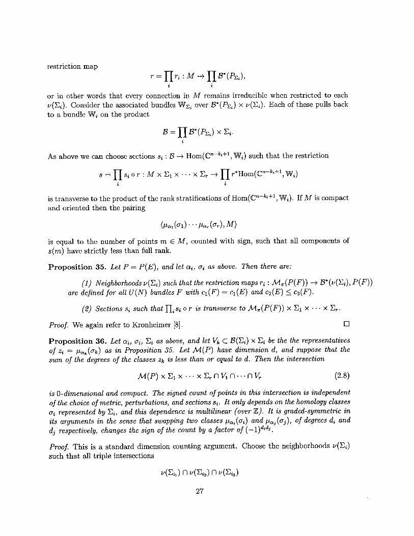
s = f si o r : M x El x --. x E, - r*Hom(Cn-k±,+W)

is transverse to the product of the rank stratifications of Hom(Cn-ki+l, Wi). If M is compact

and oriented then the pairing

(P-1 (o-1) .. -- Pa,(o-r), M)

is equal to the number of points m E M, counted with sign, such that all components of

s(m) have strictly less than full rank.

Proposition 35. Let P = P(E), and let aj, o- as above. Then there are:

(1) Neighborhoods v(i) such that the restriction maps ri : M,(P(F)) -4 B*(v(Ei), P(F))

are defined for all U(N) bundles F with c1 (F) = c1 (E) and c2 (E) < c2 ( F).

(2) Sections si such that 1 si o r is transverse to M,(P(F)) x E1 x - x E,.

Proof. We again refer to Kronheimer [8]. l

Proposition 36. Let aj, a-, EY as above, and let Vk C B(EA) x Ei be the the representatives

of zi = pa,t, ) as in Proposition 35. Let M (P) have dimension d, and suppose that the

sum of the degrees of the classes zk is less than or equal to d. Then the intersection

M(P) x Ei x ... x E, n Vi n -.. n Vr (2.8)

is 0-dimensional and compact. The signed count of points in this intersection is independent

of the choice of metric, perturbations, and sections si. It only depends on the homology classes

o-1 represented by E1, and this dependence is multilinear (over Z). It is graded-symmetric in

its arguments in the sense that swapping two classes pa, (o-) and Pa, (oj), of degrees di and

dj respectively, changes the sign of the count by a factor of (-l)didj.

Proof. This is a standard dimension counting argument. Choose the neighborhoods v(E.)

such that all triple intersections

v(Eri) n V(Ei2) nv(-i3)

27

are empty, and every double intersection involving a point class is empty as well. Any pointx E X is contained in at most two neighborhoods v(E), and at most one neighborhood suchthat E is a point. Thus for any finite set of points {X1, ... , Xk} C X, the intersection of allVi such that {y} n v(Ei) = 0 has codimension strictly larger than d - 4Nk. By Proposition35, such an intersection is disjoint from M(P(F)), where F is the bundle with c1(F) = ci(E)and c2(F) = c2 (E) - k.

Now let (An, yi,..., y,) be a sequence of points in the intersection (2.8). The connectionsAn must limit, after passing to a subsequence and bubbling at a finite set of points x,, ... Xk,to a connection Ao on P(F). But the moduli space M(P(F)) is transverse to the intersectionof all Vi such that {x} n v(Ei) = 0. In particular the set of possible limiting connections A,is empty, unless k = 0, in which case the limit lies in (2.8). This shows that the intersectionis compact.

To show graded symmetry, just observe that the only effect of swapping two factors isto change the orientation on El x ... x Er, and the effect of this change is to modify theorientation by a factor of (-1)didi.

To show independence of metric and perturbation, sections, and representatives of theEi, we apply the same argument to a 1-parameter family of moduli spaces obtained byvarying the metric and perturbation, restricting the family to neighborhoods of variouscobordisms Ei ==> E', and taking transverse sections on the configuration spaces of theseneighborhoods. We thereby obtain a compact, oriented cobordism between two sets of signedpoints, which verifies that the signed counts are equal.

The same argument also shows that the invariant is linear, because whenever we can write- = 0-'+ a" there is a homology (more precisely, a stratified cobordism) from E to the union

of E' and E".

Definition 37. Given ac and c-i as above, and a class c E H 2 (X), we define the SU(N)Donaldson invariant

Dx,c(pi0 1 (- 1 ) ... (-,))

to be the signed count of points defined in Proposition 36, viewed as a linear map

Dx,c : A(X; SU(N)) -+ Q

defined on the image of p: H*(PU(N)) 0 H<2 (X) -+ A(X; SU(N)).

There is something a bit arbitrary about our definition of Dx,c, in that we chose a par-ticular associated bundle W in the construction. We could have made the same definitionas above, replacing p, (o-x) with a combination of classes 1p133 (-rj), where the 6j are Chernclasses of a different associated bundle and the Tj are different homology classes on X (seeequation 2.7). We would like to know that such a modification results in the same mapDx,c : A(X; SU(N)) -+ Q. We can use the following refinement of our dimension countingargument to handle some cases:

Proposition 38. Let ak and U-k as above. Suppose further that all geometric representativesE,... , E,_1 are mutually disjoint (but not necessarily disjoint from E,). Then the signedcount of points in the intersection (2.8) depends only on pa,(Er) as an abstract cohomologyclass on B(P).

28

Proof. For a fixed metric and perturbation, it suffices to show that the intersection

K = M(P) x Ei X .. X Ern Vi n ---n v_

is compact, because then the signed count of points in Vr n K is just given by the cohomolog-

ical pairing (Par-(ar), [K]), which does not depend on the choice of geometric representative

for pa,(Ur).As in Proposition 36, consider a finite set of points X1 , ... , Xk E X. Because E1,... Er1

are mutually disjoint, each point xj can be contained in at most one neighborhood v(E).

Hence the intersection of all V such that {x} n v (Ei) = 0 has codimension at least d - 2Nk.

In particular, it is disjoint from the moduli space M(P(F)) with c2(F) = c2 (E) - k. To see

that K is compact, we now proceed exactly as in Proposition 36.

Clearly we can do better in cases where there are not "too many" intersections between

the Ei. However, in the simplest cases it is impossible to do better using the methods above.

For example, we might try to evaluate classes pa, (O-), [a, (0-2 ), and Pa, (0 3 ) on a 12-dimension

moduli space of SU(3) connections. If the representatives Ei each have nontrivial pairwise

intersections, then we cannot show that V2 n V3 is compact, because there might be bubbling

on E2fn 3.One way to resolve the issue is to use the blowup formula. In the next chapter we will prove

a vanishing result (Proposition 65) which implies that if E, is a sphere of self-intersection

-1, then the signed count of Proposition 38 automatically vanishes. As a consequence, we

can blow up X at all points where the Ei intersect, then replace each E with its proper

transform Ei = Ei + Ej +eij, without changing the signed count of points. We can then

replace each pa,(di) with a combination of pg (ii) in the blowup. Applying Proposition 65

again, we can eliminate all ri which intersect the exceptional curves. Blowing back down,we find that the corresponding replacement is valid on X as well.

2.3 Cylindrical Ends and Gluing

2.3.1 Cylindrical Ends

Much of our discussion of ASD moduli spaces on compact manifolds carries over to more

general noncompact manifolds.

Definition 39. We say that an oriented Riemannian 4-manifold X has asymptotically cylin-

drical ends if there is a compact subset K c X whose complement X \ K is diffeomorphic

to a product (0, oo) x Y for some 3-manifold Y, such that the metric on X \ K is given by

gx = dt 2 + gy + e-Ath(t),

where gy is a fixed metric on Y, A is a positive constant, and h(t) is a smooth bounded,t-dependent section of Sym 2 (T*Y). If h(t) is identically zero we say that W has cylindrical

ends.

To set up configuration spaces on manifolds with asymptotically cylindrical ends we need

to choose appropriate boundary conditions at infinity.

29

Definition 40. An adapted bundle (P, 77) on a 4-manifold X with asymptotically cylindricalends is a principal bundle P -+ X, together with a choice of a flat connection 77 on Ply.

Given an adapted bundle, we choose connection Ao that restricts to 21 on the cylinderY x [0, oo). We would like to define the configuration space to be the space of all connectionson X that approach q asymptotically at infinity. If q is irreducible we can imitate the compactcase exactly and define

A(P; r) = {Ao + ala E L2(X, A' 0 adP)} ,

However, when 77 is reducible this definition is inadequate. The issue is that the operatorsd*dA are not Fredholm, hence our construction of slices is invalid.

To remedy the difficulty, we need to introduce weighted norms on the space of sections ofA' 0 adP. Fix a small positive real number a, and a smooth nonvanishing function W onX such that

W(y, t) = e"t

on the cylindrical end Y x (0, oo). Define a weighted norm

a2,- = |Wa IL

and define L ',(X, A' 0 ad(P)) to be the completion of the space of smooth sections withrespect to this norm.

Definition 41. Let (P, 2) be an adapted bundle on a 4-manifold X with cylindrical ends.We define

Aa(P,7 ) = {Ao + a a E L2',(X, Al 0 adP)}.

ga(P,27 ) = {'y: X -+ G(P)17-'dAO7 E L2'a(X, A' 0 ad(P))}

B'(P,) = (Pq1G(M

When the context is clear, we will drop a and 7 from the notation.

There is a homomorphism evc : G'(P) -+ r. given by "evaluation at infinity". It isnatural to consider the kernel of this homomorphism.

Definition 42. We define the framed gauge group to be

GO"(P) = {y E Ga(P)|7. = 1}

and we define the framed configuration space to be

B"(P) = A"(P)lGo(P)

The framed gauge group is in some ways a more natural group to consider. For example, itstangent space is L 2,(X, ad(P)), which fits naturally into the framework of weighted spaces.It also acts freely on Ac(P), because a nontrivial stabilizer would evaluate nontrivially atinfinity. Thus B(P, 2) has no quotient singularities, unlike the configuration space on acompact manifold.

30

Proposition 43. 3(P, 77) is a Banach manifold with a smooth action of ]FJ7.

Proof. Let d*" denote the formal adjoint of dA with respect to the weighted norm. To

construct a slice for the action of g(P), we consider its kernel:

TA,E = {A + ald*aa = 0,|a2,. < }.

To check that this is a slice we can imitate the compact case. The key point is that d*'adAis now a Fredholm operator, provided that a is nonzero and smaller than any eigenvalue of

the operator d,*d,7 . Since 90(P) acts freely we see that B(P) is a Banach manifold with a

smooth action of ga(P)/g (P).

It remains to be shown that the homomorphism ev.. : !;(P) -+ F,, is surjective, so that

all of F, acts on g(P). The proof of Proposition 15 shows that F, is connected mod Z.

Since elements of Z extend over X, it suffices to show any y in the identity component of

F extends as well. But such an extension can be given explicitly, by homotoping Y to the

identity along the neck, then extending by the identity over the rest of X. E

Our discussion of moduli spaces and perturbations in the compact case carries over to

manifolds with asymptotically cylindrical ends.

Definition 44. Let 7r be a perturbation of the ASD equations on an adapted bundle (P, n).

We define the framed moduli space of solutions to the perturbed equations to be

M7(P) = [A] E f(P) I FA=V(A)

Proposition 45. Let P be an adapted bundle over a Riemannian 4-manifold X with asymp-

totically cylindrical ends. Then there exists a residual set of small perturbations ir, supported

in a compact subset of X, such that every A G M,(P) is regular.

Proof. The connection A is regular if and only if the cokernel of di is trivial. The proof of

Proposition 23 shows that we can choose compactly supported perturbations such that any

element of the cokernel vanishes outside of the cylindrical end. But elements of the cokernel

satisfy a unique continuation property on the cylindrical end (because they are solutions of

an ODE), and hence must vanish there as well. 0

2.3.2 The Equivariant Universal Bundle

Because connections in B(P, q) all have trivial stabilizers, there is a universal PU(N)

bundle P defined over all of ff(P, 7) x X, not just over the space of irreducible connections.

This bundle is equivariant with respect to the action of F,, so it has equivariant character-

istic classes ak(P) E Hr (B(P, i)). To compute these characteristic classes we will need a

description of the restriction of P to the orbit of a reducible connection A E 1(P, M ).

Proposition 46. Suppose that A admits a reduction of structure to a subgroup H C PU(N),

so that P = Q XH PU(N) for some H-bundle Q and A is induced by a connection on Q.

31

Then the restriction of P to the orbit 9 A = r./FA in (P) x X is isomorphic to

(X X Q) XrAxHPU(N)

as a r 7-equivariant bundle over 9 A.

Proof. By definition, the universal bundle is

P = g 0 (P)\B(P) x P = x g(p) (A(P) X P)

Restricting to the orbit of A, we have an isomorphism

, x rA P -+ P

given by sending (z, p) to (z, A, p) for any z E r,, and any p E P. Applying P = Q x H PU(N)gives

Ji, XrA P = (F77 X Q) XrAXGPU(N)

as desired.

Corollary 47. If o- C X is a cycle of positive dimension then for any a E H*(BPU(N))the equivariant classes fA&(o-) are trivial in a neighborhood of the trivial connection E.Proof. There is a neighborhood U of the orbit Oe that retracts equivariantly onto Oe, soit suffices to show that A,,(o-) is trivial on Oe. Because re = PU(N) we have H = {id},hence Proposition 46 shows that P is pulled back from an equivariant bundle on a point.Therefore,

f.(u-) = a(P)/o- = 0

as desired.

2.3.3 Index Theory

We can compute the virtual dimensions of cylindrical end moduli spaces using the excisionprinciple for indices.

Proposition 48. Let X 12 = X1 UX 2 and X 34 = X 3 UX 4 be 4-manifolds such that X 1 n X 2 =X3 n X4 = Y x (0,1) for some 3-manifold Y. Write X 14 = X 1 U X4 and X 32 = X 3 U X 2.If Di are elliptic operators on Xi that agree on Y x (0, 1), and Dij are the elliptic operatorsobtained by identifying Di and Dj over Y x (0,1), then we have

ind(D1 2) + ind(D3 4) = ind(D14) + ind(D3 2)

Proposition 49. Let V± be adapted U(N) bundles over 4-manifolds X±, with limiting flatconnections 77. Suppose that X+ has a cylindrical end Y x (0, oo), that X- has a cylindricalend Y x (-oo, 0) and that there is an isomorphism y : q+ -+ i. Let X be the closed 4-manifolds obtained by gluing together X+ and X- and let V be the bundle obtained by gluingV+ and V. Let A± be connections on X±, and let DA± be the corresponded Dirac operator,

dA: L 'a(V 0 A1) -+ L '"(V e V o A2 ).

32

viewed as an operator on weighted spaces. Then for all sufficiently small a > 0 and any

connection A on V we have

ind(DA,) + ind(DA ) = ind(DA) + ho(r) - hl(?)

where h'(71) are the ranks of the cohomology groups of Y with coefficients twisted by r.

Proof. By the excision principle, we can reduce to computing the index of the operator

(9 W'(t)Da" = a+ H77 + WtD77~ Hat W(t)

on the cylinder Y x R, where H. is the self-adjoint operator

=(0 d* \

-dn *dq '

E is the operator which acts as +1 on A' and as -1 on A', and the weight function W is

equal to e-at for negative t and eat for positive t. But the index of D' is the spectral flow

of H,7 + 4dlW e, which is equal to ho(rq) - h'(7).dt

Proposition 50. Let X be a 4-manifold with cylindrical ends, and let V be an adapted U(N)

bundle over X, with limiting flat connection i. Then there is a constant p(rq), depending only

on q, such that

ind(DA) = c(V) 2 - 2c 2 (V) + N 2 + h2() - h(i 7) + p(q)2 2

where A is any connection that restricts to r on the ends of X and c2 (V) and c1(V) 2 are

defined by Chern-Weil integrals of the curvature of A.

Proof. Given an adapted bundle V define a quantity p(V) by

p(V) = 2indDAo + cI(V) 2 - 2c 2 (V) + N(x + a) + ho(rq) - hl(,q)

Note that this formula is additive under gluing adapted bundles, by virtue of Proposition

??. It is zero for a bundle over a closed 4-manifold, by Proposition ??. Thus if W is an

adapted bundle that can be glued to V, we have

p(V) + p(W) = 0

But then if V' is another adapted bundle with limiting connection r, we have

p(V) = -p(W) = p(V'),

so p(V) only really depends on the limiting connection 77.

Note that p(7) changes sign if we reverse the orientation on the underlying 3-manifold Y.

In particular, p(rq) vanishes if r is invariant under an orientation reversing diffeomorphism.

33

Corollary 51. Let X be a 4-manifold with cylindrical ends, let P = P(V) be an adaptedPU(N) bundle over X, with limiting flat connection q. Then the formal dimension of theASD moduli space on P is

dim M(P) = 4Nc2 (V)+ (2 - 2N)c (V) 2 + (1 - N 2 ) x+ + h'(7) + h() + p(ad(T)) (2.9)2 2

and the formal dimension of the framed moduli space is

dim -(P) = 4Nc2 (V) + (2 - 2N)c1(V) 2 + (1 - N2) X + a + h() - h'(71) + p(ad(77))2 2

Proof. Simply apply Proposition 2.9 to the complexification of ad(P).

Finally, we observe that the results above remain valid for manifolds with asymptoticallycylindrical ends, because the operators in that context are homotopic to the ones used above.

2.3.4 The Gluing Theorem

To prove the blowup formula we need to have a general understanding of ASD modulispaces on a 4-manifold that is decomposed along separating 3-manifold Y. In general supposethat we can write X = X+ Uy X-, where X+ and X- are joined along their orientedboundaries OX* = tY. Let X be the 4-manifolds obtained by attaching infinite cylinders(0, oo) x Y and (-oo, 0) x Y to X+ and X-, and let XT be obtained by similarly attachingcylinders of length 2T. Given asymptotically cylindrical metrics on X (with the samelimiting metric gy) and a partition of unity /1 + #2 = 1 on the cylinder ZT = [-T, T] x Ywe can form a Riemannian 4-manifold XT = XT+ UzT XI, by joining X along ZT andsuperimposing their metrics using #. The rough idea of gluing is that as T tends to infinity,most ASD connections on XT can be described as a pair of ASD connections on the manifoldsX , plus an isomorphism of their limiting flat connections. The connections which cannotbe described in this way admit an analogous decomposition into a series of ASD connectionson infinite cylinders Zo (with the product metric dt2 + gy), plus a series of identificationsof their limiting flat connections.

Proposition 52. Let XT = X+ Uy ZT Uy X- as above, with b+(XT) > 2, and let P = P(E)be a principal bundle over XT, such that M (XT; P) has dimension less than 4N (so that it iscompact). Suppose that the 3-manifold Y carries only finitely many flat PU(N) connectionsup to gauge equivalence, each of which is regular (but possibly reducible), and that the (possiblyperturbed) cylindrical end moduli spaces M (X+; a) are regular. Then for T sufficiently large,the moduli space M (XT; P) can be covered by finitely many open sets, each of which isdiffeomorphic to an equivariant product of the form

M(XI, a,) xr, M(Zo, ai, a 2 ) Xr 2 - Xrk_1 M(Zo, ak_1, ak) X r, M(Xe, ak),

where the ac are flat connections on Y, and have stabilizers J'. Moreover, if 0- is a subspaceof X±, then the restriction of the universal bundle over M(XT) x a to such an open set is

obtained by pulling back the equivariant universal bundle over M(Xc,, ak).

34

We will not try to give a full exposition of this theorem here. References include [16], [9],[13].

35

36

Chapter 3

Higher Rank Blowup Formulas

3.1 Solutions Near a Negative Sphere

To understand the blowup formula it is useful to have a more general understanding of

how the SU(N) invariants of a 4-manifold X behave in the presence of an embedded sphere

o-, C X of negative self intersection -p. Following general principals of gluing, we consider

an open tubular neighborhood Np of such a sphere. This noncompact manifold has a single

end diffeomorphic to LP x (0, oo), where Lp = L(p, 1) is the quotient of S3 c C2 by the group

of p-th roots of unity. In this section, we will study moduli spaces of ASD connections on

the manifolds Np.

3.1.1 Regularity

In general one needs perturbations to achieve regularity of the ASD equations. However,in the case of the manifold Np, for sufficiently small p we can find a metric for which

transversality is gauranteed automatically.

Proposition 53. Let p be a sufficiently small integer (for our purposes, p K; 2). Then the

manifold Np admits a metric gp with the following properties:

(1) gp has positive scalar curvature and anti-self-dual Weyl curvature.

(2) gp decays exponentially to a product metric on (0, oo) x Lp.

Proof. Let O-1 ,o-2 , and O-3 be an orthonormal coframe field on S3, invariant under the left

action of SU(2), such that -3 is invariant under U(2). Define a metric on (0, 00) x S3 by

g = dr 2 + l +U 2

Because both o-3 and of + o2 are invariant under U(2), and L, is the quotient of S3 by a

cyclic subgroup of U(2), g descends to a metric on (0, oo) x Lp. If we furthermore demand

that A extend to a smooth odd function on all of R, satisfying A(0) = 0 and A'(0) = p, then

g will extend to a smooth metric gp on Np.

37

We now compute the Weyl curvature of the metric g, using the method of Cartan. Wechoose as an orthonormal coframe

6 = (60, 61, 62, 6 3 )T = (dr, Oc-, -2 , A-3 )T,

and compute its differential using the identities

da, = 20-2 A a 3

dO-2 = 20- A -1dO-3 = 2o A c- 2.

We find the matrix w of the Levi-Civita connection from dO by imposing the conditiond6 + w A 0 = 0. The result is:

0_0

0A'9-3

00

(A2 - 2)o-3Ac- 2

0(2 - A2 ).3

0-Ao-

-Ac- 3-AO- 2

Ac-0

The curvature matrix Q = dw + w A w is given by

)0

A-23-A/031

0603 - 2A'012

A/023

02A'6 03 + (3A 2 - 4)012

A'6 02 + A2

A1031-2A6 03 + (4 - 3A 2 )0 12

0-A'og - A2623

-- (003 - 2A'612-A/002 - A2 031

A'901 + A26230

where to save space we have used the shorthand 6ij = 9, A O. We then compute the self-dualpart of the 2-forms Q01 + Q23 , Q02 + Q31, and Q03 + Q12. The result can be written as asquare matrix,

A'+ }A2

W++ = 012 0

0A'+ 'A2

0

00

-A- 2A'+2-!A 2 ) /whose traceless part is the self-dual Weyl curvature W+. Demanding that it vanish leads usto the ordinary differential equation

A" + 6AA' + 4A3 - 4A = 0, (3.1)

and the positive scalar curvature condition leads us to the inequality

A2

A' + - > 0.2

(3.2)

The equation (3.1) has two special solutions. Namely, if A satisfies one of the ordinary

38

)

differential equations

A' = 1-A 2 (3.3)

A' = 2 - 2A 2, (3.4)

then it automatically satisfies (3.1). We can use these special solutions to find A(r) in thecases p = 1 and p = 2, respectively. When p = 1 integrating (3.3) gives

A(r) = tanh(r)

and in the case p = 2, integrating (3.4) gives

A(r) = tanh(2r).

Both of these solutions are increasing, so the corresponding metrics have positive scalarcurvature by (3.2). They rise exponentially to the limiting value A = 1, so the correspondingmetrics are asymptotically cylindrical and limit on the round metric on Lp.

I have not tried to solve the equation (3.1) explicitly for larger values of p, but numericalsolutions indicate that A is increasing if and only if p K 2, and satisfies the positive scalarcurvature inequality (3.2) if and only if p 13. 0

In fact, the computation above can be modified to show that there is a unique U(2)-invariant metric on N, with vanishing anti-self-dual Weyl curvature, up to conformal rescal-ing and reparameterization of the radial coordinate. In particular, the metrics gp are confor-mally equivalent to those described by LeBrun in [11]. It is conceivable that g, is conformallyequivalent to an asymptotically cylindrical metric with positive scalar curvature, but I havenot investigated this possibility.

Proposition 54. Every finite energy ASD connection on (Np, gp) is regular.

Proof. Consider the Dirac operator

DA = d' + d* : Q1(X, ad(P)) -> f0 (X, ad(P)) D Q+(X, ad(P)).

Given any w E Q2 (X, ad(P)), the Weitzenbock formula for DA gives us:

dA(d+)*w - VAV* W + (S, W) + (W-, w) + (FA, w)

where VA is the connection on A+(X)®ad(P) obtained by combining the Levi-Civita connec-tion on A+ with the connection A on ad(P). Since FjA = W- = 0 and S > 0, we concludethat any w in the cokernel of d+ must vanish identically. Thus for any such connectionHA = 0, as desired.

In the future we will implicitly use the metric gp when referring to ASD moduli spaces onNp. Therefore, any time we use regularity of the moduli space we will be assuming implicitlythat p is small enough so that gp has positive scalar curvature, or that there is a conformallyequivalent metric with positive scalar curvature.

39

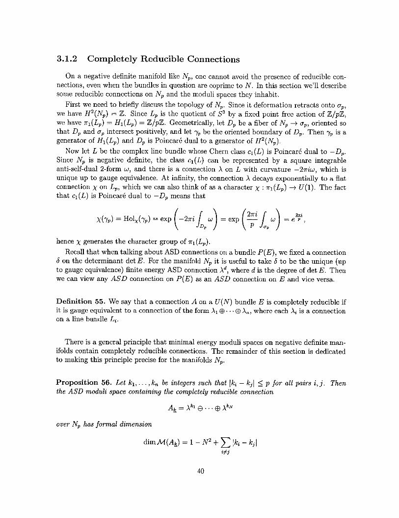
3.1.2 Completely Reducible Connections

On a negative definite manifold like Np, one cannot avoid the presence of reducible con-nections, even when the bundles in question are coprime to N. In this section we'll describesome reducible connections on Np and the moduli spaces they inhabit.

First we need to briefly discuss the topology of Np. Since it deformation retracts onto o-,we have H 2 (Np) = Z. Since Lp is the quotient of S 3 by a fixed point free action of Z/pZ,we have ir1(L,) = H1 (Lp) = Z/pZ. Geometrically, let Dp be a fiber of N - o-p, oriented sothat Dp and u, intersect positively, and let -, be the oriented boundary of Dp. Then -Y is agenerator of H 1 (Lp) and Dp is Poincare dual to a generator of H 2 (Np).

Now let L be the complex line bundle whose Chern class ci(L) is Poincar6 dual to -Dp.Since Np is negative definite, the class c1 (L) can be represented by a square integrableanti-self-dual 2-form w, and there is a connection A on L with curvature -27riw, which isunique up to gauge equivalence. At infinity, the connection A decays exponentially to a flatconnection X on LP, which we can also think of as a character X : 7ri(Lp) -+ U(1). The factthat c1 (L) is Poincar6 dual to -Dp means that

X(7y) = Hol(y (-) = exp 27ri D = exp e ,

hence X generates the character group of 7ri(Lp).

Recall that when talking about ASD connections on a bundle P(E), we fixed a connection6 on the determinant det E. For the manifold Np it is useful to take 6 to be the unique (upto gauge equivalence) finite energy ASD connection Ad, where d is the degree of det E. Thenwe can view any ASD connection on P(E) as an ASD connection on E and vice versa.

Definition 55. We say that a connection A on a U(N) bundle E is completely reducible ifit is gauge equivalent to a connection of the form A, ... @ A,,, where each Ai is a connectionon a line bundle Li.

There is a general principle that minimal energy moduli spaces on negative definite man-ifolds contain completely reducible connections. The remainder of this section is dedicatedto making this principle precise for the manifolds Np.

Proposition 56. Let k1,.... k,, be integers such that Iki - k1 5 p for all pairs i, j. Thenthe ASD moduli space containing the completely reducible connection

Ak = Aki ... e AkN

over Np has formal dimension

dimM(Ak) = 1 - N2 + Iki - kj|

40

Proof. By the index formula (2.9), we have

dim (Ak- 1:(ki - kj )2 +1 - N2 + ho(l) + p(l) + E, -ho0(xki-kj) - p(xki-kjdimM(Ag) = ____ + 2N +91 2..h~ki (

It therefore suffices to show that for any integer k with Iki p we have

ho (xk) + pxk) = 1 - 21k 2k 2p

This fact was proved by Atiyah, Patodi, and Singer in [1].

Corollary 57. Let k1 ,. . ., k,, as above, and suppose that 2p < N +1. Then the moduli space

M(Ak) has negative virtual dimension, and therefore contains no irreducible connections.

In particular, every irreducible ASD connection on Ek - Lk, E ... E LkN has energy strictly

greater than that of Ak. If 2p < N +1 + 4 then we can replace "strictly greater than" with

"greater than or equal to".

Proof. Without loss of generality, we have k1 k 2 .- - kn. Then for any fixed i, we have

Z |kj - ki| = |kn - kil pj>i

Therefore,

dim M(Ak) = 1 -N 2 +Z 2|k - kili j>i

< 1 -N 2 + 2p(N - 1)

= (2p - N - 1)(N - 1)

The right hand side of this equation is negative if 2p < N + 1, hence M (Ak) has negative

virtual dimension. If 2p < N + 1 + N, then the right hand side is less than 4N, so any

moduli space of strictly smaller energy has negative virtual dimension, hence contains no

irreducible connections.

As an application, we can compute all the minimal energy moduli spaces on CP2.

Proposition 58. Let 0 < k < N and let Ek be the U(N) bundle over N 1 with (cl(Ek) =

kc1 (L). Then the completely reducible connection

Ak = kA e (N - k)1

has energy strictly less than any other finite energy ASD connection on Ek. As a conse-

quence, the framed moduli space M(Ak) is diffeomorphic to the Grassmannian Grk(CN).

Proof. Let B be an ASD connection on Ek, and suppose that B has minimal energy among

all ASD connections. Write B = Di Bi as a sum of irreducible ASD connections on bundles

41

FR. Write c1(F) = (ki+Ndc)c1(L) with 0 < ki < N. Then by Proposition 57, the completelyreducible connection

Ai = k Adi+1 e (N - ki)Adi

has strictly less energy than Bi. Substituting Ai for Bi, we obtain a completely reducibleconnection A on Ek with strictly less energy than B. We conclude that if A has minimalenergy then it is completely reducible, so

A = Ak, e Ak2 E ...E AkN

for some integers ki. If ki - kj > 1 for any i and j, then the connection A, E A has strictlygreater energy than Aki+1 E Aki-1. Since A has minimal energy, this implies that Iki - kyj 1for all i and j, hence A = Ak.

The description of the framed moduli space then follows from the fact the stabilizer ofAk is rk = S(U(k) x U(n - k)), hence its orbit in M(Ak) is Grk(CN) = SU(N)/S(U(k) xU(N - k)). l

Note that the argument above fails if p > 1, because the inequality 2p < N + 1 does nothold for all N. However, the weaker inequality 2p < N + 1 + 4N is valid for all N as longas p < 4. In this regime we can therefore hope to partially salvage Proposition 58.

Before proceeding, we need to establish some notation. Let 0 < r1 < ... rN < p beintegers, and consider-the flat connection

7 r = X e Xr2 D ... D XrN

on LP. Let r = r1 + - + rN, so that c1(2jr) = rc1 (L). If E is an adapted bundle on Np withlimiting flat connection ?7r, then we necessarily have

(c,(E), o-,) =- r mod p.

If E satisfies this constraint, we say that it is admissible for 7r.

Proposition 59. Let E be a vector bundle over Np. Then E admits a completely reducibleASD connection, satisfying the hypotheses of Proposition 57.

Proof. Define a connection

Ar's = Ara ®D ... (1 ArN eD A l+p.. eD A r.-i+p

and call the underlying bundle of this connectionruns from 1 to N we obtain all admissible valuess and some integer d we have E = Ld 0 E,, soconnection Ad 0 Ar,s.

E,. Then c1(E,) = (r +ps)c1(L), so as sof ci(E) mod N. In particular, for someE admits the completely reducible ASD

El

Proposition 60. Suppose that p 4. Let E be a U(N) bundle on N,finite energy ASD connection on E, which limits on a flat connection Lyr.completely reducible ASD connection A on E, also with limiting value 7,less than or equal to that of B.

and let B be aThen there is awhose energy is

42

Proof. Write B = Ei Bi, where each Bi is an irreducible ASD connection on a bundle F ofdimension ni. Each F admits a completely reducible connection Ai = Ar. ,,,, which satisfies

the hypotheses of Proposition 57. Because p < 4, the inequality

4ii2p < n + 1 + 4n

n -1

holds for all n > 2. Since Bi is irreducible, we conclude that it has energy greater than orequal to that of Ai. Therefore the completely reducible connection A = Ei Ai has energyless than or equal to that of B, as desired.

It is unknown to the author whether Proposition 60 holds for all p. As an example of thedifficulties involved, let E be the trivial SU(2) bundle over N13, and let A be the connectionA-3 @A 3, which has limiting flat connection q = x3 ( X"i. Then A has minimal energy amongall reducibles limiting on i, but the moduli space containing A has virtual dimension 9. Itis conceivable that the moduli space of virtual dimension 1 is always empty in this case, butproving it would require more subtle methods and might depend on the choice of metric on

N 13 -In the case p = 2 we can explicitly write down the completely reducible connections of

minimal energy.

Proposition 61. Let Ek be the U(N) bundle over N 2 with cl(Ek) = kc1(L). Then

A= A ((N - r) E r-kA-1 r >kk- 2 E rA E (N -k r)1 k > r

has minimal energy among all ASD connections on Ek with limiting flat connection r, =

rX E (N - r)1, and it is the unique completely reducible connection with this property.

Proof. By Proposition 60 we only need to show that this connection has less energy thanany other completely reducible connection on Ek limiting on 7,.. So, let

A = A kiD.A kn

be completely reducible. Write ri = 1 for i < r and ri = 0 for i > r, and without loss ofgenerality write ki = ri + 2di. With k = E ki fixed, the energy of A is proportional to

c2 (A) - 2c 1 (A) 2 = Eki. (3.5)

In the case k > r, we rewrite (3.5) using the identity r2 = ri:

c2(A) - 2c(A)2 = r + Zk2 + (ri - 1)2 - 1 (3.6)

Because k2 and ri are congruent mod 2, each term on the right hand side of (3.6) is positive,hence

c2(A) - 2c 1 (A) 2 > r.

43

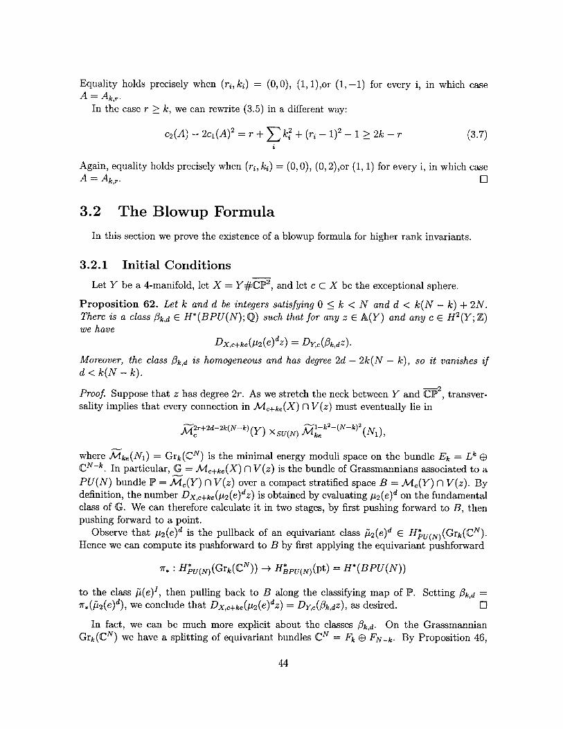
Equality holds precisely when (ri, ki) = (0, 0), (1, 1),or (1, -1) for every i, in which caseA = Ak,r.

In the case r > k, we can rewrite (3.5) in a different way:

c2(A) - 2c 1 (A) 2 = r + E k2 + (ri - 1)2 - 1 > 2k - r (3.7)

Again, equality holds precisely when (ri, ki) = (0, 0), (0, 2),or (1, 1) for every i, in which caseA = Ak,r.

3.2 The Blowup Formula

In this section we prove the existence of a blowup formula for higher rank invariants.

3.2.1 Initial Conditions

Let Y be a 4-manifold, let X = Y#Cp 2 , and let e C X be the exceptional sphere.

Proposition 62. Let k and d be integers satisfying 0 ; k < N and d < k(N - k) + 2N.There is a class 8 k,dE H*(BPU(N); Q) such that for any z E A(Y) and any c E H 2(y; Z)we have

Dx,c+ke(A 2 (e)dz) = Dyc(/k,dz).

Moreover, the class Ok,d is homogeneous and has degree 2d - 2k(N - k), so it vanishes ifd < k(N - k).

Proof. Suppose that z has degree 2r. As we stretch the neck between Y and CAP , transver-sality implies that every connection in Mc+ke(X) n V(z) must eventually lie in

fM~2r+2d-2k(N-k)(y) X SU(N) k2 -(N-k) 2 (Ni)

where Mke(Ni) = Grk(CN) is the minimal energy moduli space on the bundle Ek - Lk kCN-k. In particular, G = Mc+ke(X) n V(z) is the bundle of Grassmannians associated to a

PU(N) bundle P = Mc(Y) n V(z) over a compact stratified space B = Mc(Y) n V(z). Bydefinition, the number Dx,c+ke(p 2 (e)dz) is obtained by evaluating P 2 (e)d on the fundamentalclass of G. We can therefore calculate it in two stages, by first pushing forward to B, thenpushing forward to a point.

Observe that p2 (e)d is the pullback of an equivariant class A 2 (e)d E H U(N)(Grk(CN).Hence we can compute its pushforward to B by first applying the equivariant pushforward

7r* : H U(N)(Grk(CN)) - PU(N)(pt) = H*(BPU(N))

to the class ft(e)', then pulling back to B along the classifying map of P. Setting fk,d =7r*(A2(e)d), we conclude that Dx,c+ke(p 2 (e)dz) = Dyc(k,dz), as desired.

In fact, we can be much more explicit about the classes 6k,d. On the GrassmannianGrk(CN) we have a splitting of equivariant bundles CN = Fk E FN-k. By Proposition 46,

44

the universal bundle over Mc+ke(X) x e is the projectivization of the vector bundle

V = (L 0 Fk) ( FN-k-

We can easily compute the Chern character of this bundle,

Ch(V) = exp(L)Ch(F) + Ch(F_-k)

and from this we can obtain the classes a 2 (P), from the formula

a2 (P) = -[exp (kL) Ch(V)] 2-

Slanting with e, we get

N -k k=2(e) = N cl(Fk) - c1 (Fnk) = c1(Fk).

N N

We are therefore reduced to computing the equivariant pushforward

#6k,d = c1(FedIGrk(CN)

which is straightforward for any particular values of k and d. For example, Kronheimer

proved that 31,N-1 = 1 and used this to define higher rank invariants in the case where c is

not coprime to N. In more generality, we have:

Proposition 63. The class /k,d is a nonzero integer when d = k(N - k). In particular we

have OO = 81,N-1 = 1.

Proof. The class cl(F) is represented by a section of an ample line bundle on the complex

projective variety Grk(CN), hence the integral of cl(Fk)k(N-k) is nonzero. In the case k = 0

we have #o,0 = +1 trivially. In the case k - 1 we are evaluating the top power of the

hyperplane class on CpN-1, hence we get 01,N-1 = ±1. For evaluation of the sign we refer

Kronheimer [8]. E

The vanishing criterion in Proposition 62 generalizes as follows, with the same proof:

Proposition 64. Let 0 < k < N and let I = (i2 , - - -, iN) be a multi-index satisfying

0 < dim(I) = 2i 2 + 4i 3 + -.. + (2N - 2)iN < 2k(N - k) + 4N.

Then there is a class fk,I E H*(BPU(N); Q) such that for any z E A(Y), and any c E

H 2(Y; Z) we have

Dx,c+ke(p(e)'z) = Dx,c+ke (/2(e)i2 ... [N(e)iNz) = Dyc(#k,Jz)

If dim(I) < 2k(N - k) then fA,I = 0.

There is another vanishing condition in the case k = 0.

45

Proposition 65. Let I = (i 2 , - - -, iN) be a multi-index satisfying

0 < dim(I) = 2i 2 +4i 3 + +(2N - 2)iN< 4N.

Then /k,I = 0.

Proof. The classes pi(e) vanish in a neighborhood of the trivial connection by Proposition46 , hence do not intersect the moduli space Ii-N 2 (N1 ). Thus for a sufficiently long neckthey do not intersect the moduli space Mdim(I) (X). El

3.2.2 A Simple Relation

In this section, we consider a 4-manifold X that contains a sphere a of self-intersection-2. Such a 4-manifold can be written as X = Y UL2 N2 for some Y with DY = L2 . In thissection we will use our understanding of the minimal energy moduli spaces on N2 derive asimple relationship between the invariants Dx,,+, and Dx,c.

Proposition 66. Let MO,2 be the moduli space containing the connection AO, 2 = A e A~ 1 e(N - 2)1 of Proposition 61. Then every connection A E MO,2 takes the form

A = B E (N - 2)1

for some rank 2 connection B.

Proof. Write A = Ei miAi as a sum of irreducible connections of dimension ni, each havingmultiplicity mi. Then the orbit of A in M 0 ,2 has dimension

d = 22 + (N - 2)2 - m2

On the other hand, by Proposition 56, the moduli space M0O,2 has dimension 4. Therefore,

mi > (N - 2)2

If one of the Ai has dimension at least 3, or if two of the Ai have dimension at least 2, thenEZ mi N - 2, hence

Zmi (Zmi) 2 < (N-2)2

The first inequality is strict unless there is a single term in the sum, in which case the secondinequality is strict. We conclude that A = BD C, where C is completely reducible. We knowthat there is a reducible Bo = Ar E A' with the same energy as B. By Proposition 61, theconnection A' D A' D C has to be AO, 2, so either B 0 = A E A- or B 0 = A'' ( 1. In the lattercase, B cannot be irreducible, because it lives in a moduli space of negative dimension. Weconclude that either A = A2 ,0 or C is trivial, which completes the proof. l

Proposition 67. The SU(2) moduli space MO,2 consists of a half-infinite segment [0, oo),plus a union of finitely many circles and infinite segments (-cc, oo). The corresponding

46

components of the framed moduli space MO,2 are equivariantly diffeomorphic to T*(S 2),SO(3) x S', and SO(3) x R, respectively.

Proof. The space of irreducible connections M0,2 is a smooth 1-manifold with two kinds of

ends. First, there is the reducible connection A E A- 1. Second, there are limits where energy

slides off the end of N 2 . The latter take the form F#6, where E is the trivial connection

and F is one of finitely many connections F 1 , .. . , F,, on L 2 x R. Exactly one component of

MO,2 joins A E A- 1 to one of the Fi#O. The other components are either compact (circles)

or they join two of the Fi#E).To show that the component of the framed moduli space lying over [0, oo) is diffeomorphic

to T*(S 2 ), it suffices to show that the normal bundle to the orbit of A e A 1 has degree ±2.

But this is clear, because the link of the orbit is SO(3) = L 2 .

We now prove the simple relation promised above. In the case N = 2 this result is due

to Ruberman [15].

Proposition 68. For any c E H 2 (Y) and any z E A(Y) we have

Dx,c(p2 (a)2Z) = ENDx,c,+(2z),

where EN is a universal sign given by

f+1 N = 2 mod 4EN - 1 N odd

Proof. First we describe how to compute the left hand side of the equation. From Proposi-

tions 61 and 56, we see that the framed moduli space MO,2,. has dimension 4r 2 . Since A 2 (U-) 2

has degree 4, the only moduli spaces we encounter as we stretch the neck are Mo,o and M 0 ,2 .

Since M 0 ,0 only contains the trivial connection, it does not intersect any V(pi(o)). Hence

all intersections take place on an open subset of M2d+4 (X) diffeomorphic to

U = MC[r 2] Xr MO, 2 ,

where IF = S(U(2) x U(N - 2)) is the stabilizer of rqO, 2 -

We can compute the universal bundle over MO,2 x -, using Proposition 46. Note that the

stabilizer of any connection in MO,2 is a subgroup of S(U(1) x U(1) x U(N - 2)). Hence

there are line bundles P and Q, and a rank N - 2 vector bundle F over Mo,2 , such that the

universal bundle is the projectivization of

V = (L ® P) ( (L-1 0 Q) e F.

Away from AO, 2 the stabilizers reduce to S(U(1) 2 x U(N)), hence the line bundles P and

Q become isomorphic. Writing p = c1 (P) and q = c1 (Q), we conclude that p - q is supported

in a neighborhood of the orbit of AO, 2 . On the orbit of AO, 2 , which is a 2-sphere, P is a degree

one line bundle and Q is its inverse. Therefore,

((p - q) 2,7M o, 2 ) = +2

47

with the sign depending on how we orient MO,2.

Now, the Chern character of V is given by

Ch(V) = exp(l) exp(p) + exp(-l) exp(q) + Ch(F).

From this formula we can compute a 2 (P) and pi2 (0). Slanting both sides by a, we obtain

12(a)=p - q

from which it follows that Dx,,(pi2 (a)2z) = ±2n, where c is a universal sign and n is thesigned count of points in M2dc[q 2] n V(z).

The left hand side is easier to compute. Indeed, the moduli spaces M2,2r all have positive

dimension, except for M 2 ,2 , which has dimension 0 and consists of a single connection A 2,2 .Stretching the neck, we conclude that the moduli space Mid(X) n V(z) consists of a singleconnection for each point in M2dc[772] f V(z). Therefore,

2Dc+,(z) = t2n = EDX,c(p2(U)2Z)

for some choice of sign e.

To compute E, let Y be a 4-manifold with Dyc(z) = 1 for some c and z. Let X be themanifold obtained by blowing up Y twice. Then we have

Dx,c+ke1+le2 ( 2 (eA k(N-k) 2 (e)l(N-lz) = k1

for some nonzero integers #k and #1. The result we have proved so far shows that

Dc+kel+ke2 (/L2(el - e2 )2pA2 (el + e 2 ) 2k(N-k)-2) = 2EDc+(k+)el+(k-1)e 2 (/p2(el + e 2 )k(N-k)-2)

= 2 EDc+(k+)e+(k-1)e 2 (/.12(el + e 2 )(k+1)(N-k-1)+(k-1)(N-k+1))_ (3.8)

Assume that k is strictly between 0 and N, and expand out both sides. For dimensionreasons there is only one nonzero term on either side. Examining this term shows that

-sign('32) = E -sign( 3 k+1k-1)

Since #% and 31 are both positive we conclude that

sign(#k) =

On the other hand, we also have

3k = Dc+ke(P 2 ( )k(N-k)Z)

= Dc-ke( 1 2 (e)k(N-k)Z)

= -ENDc+(N-k)e(P2 ek(N-k)Z)

= (-1)(k(N-k)+l) ENN-k-

48

Combining these two pieces of information we see that

(-e)J+[Y&J = (_l)(k(N-k)+l)EN-

If N is odd then the right hand side is +1 for all k, hence E = 1. If N is congruent to 2 mod

4 then setting k = 1 gives e = EN = -1.

3.2.3 Partial Blowup Functions

Using the simple relation of Proposition 68, we can extend Proposition 62 to arbitrary

values of d.

Proposition 69. Let Y be a 4-manifold with bj > 1 and let X be its blowup. Then for

every integer k there exists a formal power series Bk(t) = Ed bk,dL E H*(BPU(N); Q[[til)

such that for any c E H 2(Y) and any z E A(Y) we have

Dx,c+ke(exp(P2(e)t)z) = Dx,c(Bk(t)z)

Proof. Let X be the manifold obtained by blowing up Y twice, and let el, e2 be the excep-

tional spheres. Then the simple relation tells us

Dx,c+kei+ke2 (I2(ei--e2 )2 exp(tP2 (e1)+tA2 (e2))) = 2 ENDx,c+(k+1)e+(k-1)e 2 (exp(ty 2(ei)+tp2 (e2 )))(3.9)

Expanding in powers of t gives us an infinite series of relations between the invariants

Dx,c+ke(2(e)d). We want to see that these relations can be solved recursively, by induction

on d.

To see why a solution exists, it is convenient to think of the relations as a system of dif-

ferential equations to be satisfied by the functions Bk(t). Solving these differential equations

order by order in t, given suitable initial conditions, is equivalent to using (3.9) to inductively

find acceptable values for bk,d. Explicitly, the differential equations we must solve read as

follows:B'Bk - B B1 = ENBk+1Bkl.

When k is a multiple of N we have Bk(O) = +1, so examining the coefficient of td always

allows us to solve for bo,d and bN,d in terms of coefficients bk,e with e < d. It therefore remains

to solve for the rest of the bk,d in terms of bo,d, bN,d, and lower order terms.

Unfortunately, for 0 < k < N the equations are degenerate, because Bk(O) = 0. To

remove the degeneracy, we can write

Bk(t) = bktk(N-k)fk(t)

for some power series fk satisfying fk(0) = 1. By Proposition 63, we can take the coefficients

bk to be nonzero integers. Rewriting our differential equations in terms of the fk we see that

b2t 2 (fk'fk - fklfkl) = k(N - k)b2 f2 - ENbk+lbk-lfk+lfk-l-

49

Setting t = 0 in this equation gives the identity

k(N - k)b2 = ENbk+1bk-1

so we can eliminate b2 and EN from the equations, obtaining

t2(fl'fk - fklfi) = k(N - k)(fk - fk+lfk-1).

This equation is still degenerate, but we can understand the degeneracy in a precise way.Collecting terms of order td, we get a system of equations

fkd = k(N - k) 2 fkd - fk+,d - 1k-1,d + lower order terms(d -2)! d

which can be rewritten as follows:

2 fk,d - fk+1,d - fk-1,d d(d - 1)2 2k(N - k) k'd =k.

The left hand side can be viewed as a linear operator L : RN+1 _+ RN-1, and we must showthat this operator is surjective for fixed values of fo and fN. To do so it is sufficient torestrict to fo = fN = 0, in which case L becomes a symmetric operator with correspondingquadratic form

N-1 N-1

QM= N(fk+ - fk)2 kk

k=O k=1

It therefore suffices to show that Q is negative definite for sufficiently large d. But

n-1 N-1 dd-1Q(f) E 2(f+1 + f ) k(N - k) k

- ( 4 d(d - 1) 2I: 2k(N - k)J k

k=1

so Q will be negative definite provided

d(d -1)> 4

2k(N-k)

for all k between 0 and N. This inequality is automatically satisfied if d > N. In the ranged < N, Proposition 62 already provides us with values for fk,d = bk,k(N-k)+d- Using thesevalues as initial conditions, we can solve for a blowup function Bk(t) to all orders in t. 0

Definition 70. Any function Bk(t) which correctly computes the invariants Dx,c(p 2 (e)dz)as in Proposition 69 is called a partial blowup function.

Note that we make no claims about the uniqueness of the functions Bk(t). However, thedifference of two partial blowup functions vanishes inside the Donaldson invariant of any 4-manifold, so one could in principle prove uniqueness by finding 4-manifolds that distinguish

50

all classes in H*(BPU(N)), or by viewing the blowup function as taking values in a suitableFloer homology theory.

Finally, it is worth remarking on the differential equations satisfied by the partial blowupfunctions,

BI'Bk - BIBL = ENBk+1Bk.

If we make the substitution

Uk = log( fEN Bk

then this system of equations becomes

d2

dt2 - ek1k-ekk

which is known in mathematical physics as the Toda lattice. It describes a periodic chain

of particles, each of which interacts with its neighbors via an exponential potential function.

A relationship between the Toda lattice and the SU(N) blowup function was predicted byMarifio and Moore in [12], so Proposition 69 can be seen as a confirmation of physicists'

expectations about the behavior of higher rank invariants.

3.2.4 Full Blowup Functions

We call the Bk(t) partial blowup functions because they only allow us to calculate invari-

ants of the form Dx,c(p 2 (e)dz). The full SU(N) blowup function would be a power series in

N - 1 variables t2 ,..., tN such that

Dx,c(exp(t2 P2 (e) + --- + tnin(e)) = Dx,c(B(t 2, ... , tN))

In this section we will prove that a full blowup function exists for N < 4, and study the full

blowup function in detail when N = 3 and k = 0.

To extend the recursion of Proposition 68 to arbitrary classes pi(o), we again consider a

4-manifold X containing a sphere o- of self-intersection -2, and we write X as Y UL2 N 2.

Proposition 71. Let I = (i2 , - - -, iN) be a multi-index with dim(I) = 2p < min(16, 4N).Then there exist universal aij E H*(BPU(N); Q) such that for any c E H 2 (Y, Y) and any

z E A(Y) we have

Dx,c(p(o)'z) = [ Dx,c(ai,jpi (o-)p (o-)z)).i+jip

Proof. We proceed as in 68. In the moduli space M 2d+ 2P(X) all intersections with V(z) take

place iniU = M2d+2p(y) [, 2 ] Xr MO, 2 ,

where IF = S(U(2) x U(N - 2)) is the stabilizer of NO,2. As before, the universal bundle is

the projectivization of the vector bundle

V = LP D L-1 Q D F,

51

where P and Q are line bundles that are isomorphic away from AO, 2 .The Chern character of V is given by

Ch(LP D L~ 1Q E F) = exp(l) exp(p) + exp(-l) exp(q) + Ch(F).

From this formula we can extract concrete expressions for ak(P) and pk(u), by writing theclasses ak(P) in terms of Ch(V). A nice way to organize the computation is to introduceclasses

Vk = p(k-1)!Chk(-) = (k - 1)!Ch (V)/-.

Because the classes Chk generate HsU(N) we know that each vk is a linear combination of theclasses pi(o), with coefficients in HSU(N). Hence we can replace pi(a) by vi in the statementof the theorem.

Explicitly, Vk is given by

(k - 1)!Chk(V)/- = Pk-1 - qk-1 = (p - q)sk-2,

where Sk-2 is the sum of all monomials of degree k - 2. In particular, each product vk v isdivisible by (p - q) 2 , hence is a multiple (over Hf) of the equivariant fundamental class ofT*(S 2 )_

We must therefore show that the classes sisj form a basis for H* over HsU(N). To provethis, observe that BF fibers over BSU(N), with fiber Gr 2(CN). It therefore suffices to showthat the sisj restrict to a basis for the cohomology of Gr 2(CN). But it is well known thatthe Schur polynomials

, p -p qform a basis, and these can be expressed in terms of the sisj by the identity

sk,1 = skS+1 - Sk+1Sl

Because of the restriction on dim(I), Proposition 71 only produces 9 identities, which canbe derived from the following relations between the vk:

Degree 8 v2 = 4v 2v4 - 3v3

Degree 10 -v7- = 3v 2v5 - 2v3v4

Degree 12 vTv4 = U2v6- 3v v5 + v42

vl2 2 = 2v 2v 6 + v3 v 5 +2z2

v2= 6v2v6 - 15v3 v5 - 2v4

Degree 14 v5 = v7- 3v3 v 6 + v4v5

v2v3v4 = 2v2v7 - v 4 v5

32v1 = -3v2v 7 - 9vv 6 + 9v 4v5

v2v3 = 5v2v7-9v3v6+55v4v5

52

We can replace each vi above with a combination of pi(o-) using the following table:

k (k - 1)!Chk Vk = /L(k-1)!Chk (a)

2 -a 2 -L 2 (0-)

3 a3 A3(0r)

4 a - a4 a2 P2 (0) - 4(-)

5 -a 2a 3 + a5 a3P2(0-) - a2P3(0-) + s(0-)

6 -- !a3 + 1a2 + a2a4 - a6 (a4 - a2)[ 2 (0) + a3P3 (0-) + a2 4 (U) - /1 '

In the case N = 3 there only 2 identities, which we write out for convenience.

Corollary 72. Let N = 3. Then for all c E H 2(Y) and all z E A(Y) we have

Dx,c(a 2 (o-)4z) = -4Dx,c(a 2i2 (0-)2z) - 3Dx,c(P3 (0-)2z) (3.10)

Dx,c(P2 (0) 3i' 3 ( u-)z) = -3Dx,c(a112 (o) 2z) - Dx,c(a2A2(0-)P3(U-)z) (3.11)

We can now prove the existence of a full blowup function when N < 4.

Proposition 73. Let N be 3 or 4. Then there is a formal power series B = B(t 2 , ... ,tN) E

H*(BPU(N);Q[[t 2 , . . . ,tN1]) such that for all c E H 2 (Y) and z G A(Y) we have

Dx,c(exp(t2 [t2 (e) + - -- + tNIpN(e))z) = Dx,c(B(t 2 ,. . . , tN)z)

Proof. We proceed as in Proposition 69, by blowing up twice and using the identities pro-

duced in Proposition 71. The strategy of the induction is to eliminate all powers of p3(e) and

N4(e), thereby expressing the full blowup function in terms of the partial blowup functions.

For example, suppose N = 3. Then B(0) = 1, and B must satisfy two differential

equations:

3(BB33 - B 3B 3) = -B 22 22 B + 4B 222 B 2 - 3B 22 B 22 - 4a2(B 22B - B 2 B 2 )

B2223B - 2B 2 2 3 B 2 - 2B 2 2 2 B 3 + 3B 2 2 B 2 3 = -3a 3(B 22B - B 2B 2) - a2(B 23B - B 2 B 3 )

Expanding these equations to all orders in t, it becomes clear that we can solve for all

partial derivatives of B in terms of B 223 ,B 2 3 ,B 3 , and the coefficients of the partial blowup

function that are already known. In fact, the vanishing theorem of Proposition 65 shows

that B 2 2 3 = B 2 3 = B 3 = 0, so knowledge of the partial blowup function is sufficient.

The case N = 4 is similar, but involves using 8 of the 9 equations from Section 3.2.4. E

We have not attempted to prove the existence of a full blowup function Bk(t2, ... , tN) here

because the vanishing of Bk(0) means the equations are degenerate, and a precise analysis

of the degeneracy is quite complicated.

53

3.3 The Case N=3

3.3.1 Theta Functions on a Genus 2 Jacobian

Definition 74. Let A c C9 be a full lattice. We say that an entire function 0 : C9 -+ Cis quasiperiodic with respect to A if for every A E A there exist constants aA E Hom(C9, C)and bA E C such that

O(x + A) = eax+b\O(x)

for all x E C9.

For example, any Gaussian f(x) = exTAx+bTx+c is periodic. So is the Riemann thetafunction

6(z) = E e"inTn e27inTz

nEZ9

if the lattice takes the form A = Z9 D 7Z9 for Q a symmetric matrix with positive definiteimaginary part. If two quasiperiodic functions have the same automorphy factors aA,bA,then any linear combination of them is quasiperiodic, with the same automorphy factors.The product of any two quasiperiodic functions is quasiperiodic, with the product of thetwo automorphy factors. A linear map followed by a quasiperiodic function is quasiperiodic,with respect to a different lattice.

Note that we can regard any quasiperiodic function as a section of a certain line bundleover C/A, whose transition maps can be derived from the automorphy factors. We will usecapital letters to denote the line bundle corresponding to a set of automorphy factors, so if6 is quasiperiodic, we will say that it is a section of the line bundle E.

Definition 75. Let 9(x) be an analytic function on C9. We define the Hirota differentials0[I](x) to be the unique functions such that

(x +t)(x -t) t0[I](x)

where the sum ranges over all multi-indices I= (ii, ... , ig). In other words,

0[I](x) = 0(x +t)(x -t)t=0

Proposition 76. The Hirota differentials of an arbitrary analytic (or Co) function 6 satisfythe following properties:

1. 0[I] = 0 if I has odd degree.

2. 0 [ij] =2ai log 0

3. 0[ijkl] = 2aijkI log 0+ 4 (O4j log 0 - Oki logO + 0 log -O10 log 0+ log 0 k log 0)

Proof. Straightforward computation.

54

Proposition 77. Let 9 be a quasiperiodic function with respect to a full lattice A C C9, so

that it defines a section of a line bundle E. Then for any fixed t E C9 the function

#t(x)= (x +t)(x -t)

is a section of 2E.

Proof. By definition, sections of E correspond to quasiperiodic functions 0 satisfying iden-

tities4(x + A) = ea\x+b\b(x)

for every A E A. Thus sections of 2E correspond to those satisfying

O4x + A) = e 2a,\x 2 b(OW

It is then straightforward to check that this identity is satisfied by #t.

Corollary 78. If 9 is a quasiperiodic function, then its Hirota differentials 0[I] are all

sections of 2E.

Proof. Since 9(x + t)9(x - t) is quasiperiodic in x, so are all its derivatives with respect to

t. 0

Proposition 79. Let E be a curve of genus 2, and let 9 be the Riemann theta function on its

Jacobian JE. Then the Hirota differentials 0[I] with deg I = 0,2 form a basis of H 0 (JE, 2E).

Proof. Translating and multiplying by a Gaussian, we can assume 9 is an even function

whose Hessian vanishes at the origin. In this case it suffices to prove that the 3 components

of the logarithmic Hessian of 9 are linearly independent. If there were a linear relation, then

we would have oo9, log 9 = 0 for some vectors v and w. But this implies that an irreducible

component of the zero locus of 9 is invariant under a 1-parameter group of translations,which is absurd since the zero locus is a genus 2 curve. U

Corollary 80. The Riemann theta function on JE satisfies a system of differential equations

of the form:9[ijkl] = 2Aijkli 2 + C i [pq]

pq

or equivalently,

Pijk + 2 (PijPki + PikPjil + PiPik) = Aijkl + ij Pqpq

where P, = a1 log 9.

Proof. By Proposition 76, we know that the left hand side is a ratio where # is a

section of 2E. By Proposition 79, # is a linear combination of Hirota difkerentials of order

< 2. Dividing by 92 and applying Proposition 76 again, the system of equations follows. U

55

Observe that if 6(x) satisfies a system of the above form, then so does

eXTAx+bx+c (Mx + t)

for any matrices A, C, covector b and constants c, t. In other words, multiplying by aGaussian and precomposing with an affine transformation preserves the form of the equa-tions. Ignoring this ambiguity, we can show that the Riemann theta function is characterizedby the above system of equations. More precisely:

Proposition 81. Suppose that 0 is a function whose logarithmic derivatives satisfy a systemof equations of the form:

Pill, + 6P 1 = All,, + G2 P - 2G 1 P 12 + GoP22

P 11 12 + 6P1 1 P12 = A1112 + G3 P1 - 2G 2P 12 + G1 P22

P1 122 + 2P1 1 P22 + 4P 2 = A112 2 + G4 P1n - 2G 3 P 12 + G 2P22

P1222 + 6P 12 P22 = A 1 22 2 + G5 P1 - 2G 4 P12 + G3 P22

P2222 + 6P22 = A 2 22 2 + G6Pnl - 2G 5 P12 + G4 P22

that the coefficients AijkI are given by:

All,, = 1 (GoG4 - 4G1G + 3G 2

1A 1112 = - (GoG5 - 3G1 G4 + 2G 2 G3 )6

1A11 2 2 = 1 (GoG 6 - 9G 2G4 + 8G 2

1A1 2 2 2 = - (G1G6 - 3G 2G5 + 2G 3 G4 )6

12A2 2 2 2 = 3 (G2G6- 2GG5+ 3G4)

and that 0 is not itself a Gaussian. Suppose, moreover, that the homogeneous polynomial

G(x,y)= 2 G ij

i+j=6

has exactly 6 nondegenerate zeroes in Pl. Then, up to a multiplying by a Gaussian andprecomposing with an affine transformation, 6 is the Riemann theta function on the Jacobianof the hyperelliptic curve

y2 = g(x) = G(x, 1)

Proof. This is proved in Baker [2]. To give some sense of what is involved in the argument, wewill explain how to recover the hyperelliptic curve. The idea is as follows. First differentiateeach of the 5 equations above with respect to each of the two variables. This yields a set ofequations like:

P11112 + 12P11P11 2 = G2Pn2 - 2G 1 P122 + G0 P222

56

If we eliminate all 5th derivatives, we are left with system of 4 equations of the form:

MilP111 + Mi2P112 + Mi3P122 + Mi4P222 = 0

where the coefficients Mij lie in H0 (JE, 26). Since 0 is not a Gaussian, at least one ofthe Pik is nonzero. Hence the 4 sections of H0(JE, 26) satisfy a nondegenerate degree 4equation,

det M = 0

This is the equation of the Kummer surface in P3. When we intersect it with the plane atinfinity (i.e. the image of the theta divisor) we get a doubled conic. The Kummer surfacehas six singular points along this conic, which an explicit computation shows are preciselythe roots of G(x, y). El

We also need to make a remark about initial conditions. Clearly the function P is deter-mined by P1 (0) for Il < 3. But as a consequence of Proposition 81, these initial conditionsare subject to the constraint that the second derivatives must lie on the Kummer surface.There is, of course, no constraint on the zeroth or first derivatives, since they can be mod-ified by multiplying by an exponential, which does not change the equations. Finally, it isproved in Baker that the third derivatives can be expressed in terms of the lower derivatives,which gives some actual constraints on the set of valid initial conditions. In the case wherethe initial conditions are finite and specify a singular point of the Kummer surface, theseconstraints simply say that the function 9 is (up to third order) an even function times anexponential.

3.3.2 The Blowup Function

Theorem 82. The SU(3) blowup function is a quasiperiodic function on the Jacobian of thehyperelliptic curve

y2 = (X3 + a2x + a3 )2 - 4.

Proof. By Corollary 72

B2222B - 4B 2 2 2B 2 + 3B22B22 = -4a 2 (B22B - B 2B 2) - 3(B 33B - B3B3)

B2223B - 3B223B2 - B222B 3 + 3B 22 B 23 = -3a 3(B 22 - B 2B 2) - a2 (B23B - B2B3)

and setting Q = log B we get

Q2222 + 6Q22 = - 4a 2Q 2 2 - 3Q33

Q2223 + 6Q22Q23 = - 3a 3Q2 2 - a2Q23

which look similar to the first 2 of the 5 equations satisfied by the Riemann theta function.

In fact, if we suppose that Q satisfies such a system of 5 equations, there is a unique choice

of coefficients for the remaining three equations that is consistent with the initial conditionsderived in Section 4. In total the five equations read:

Q2 + 6Q$2 = - 4a 2Q 2 2 - 3Q33

57

Q2223 + 6Q22Q23 = - 3a3Q 22 - a2Q23Q2233 + 2Q22Q33 + 4Q23Q23 = 2 - 3a3Q 23 - a2Q 33

Q2333 + 6Q23Q33 = - a 2a 3Q 22 + a Q 23 - 3a3Q 33

Q3333 + 6Q 3 = - 2a 2 - (12 + 3a)Q 22 + 2a 2a 3Q 23 + a2Q 33

These equations are not quite in the form required by Proposition 81. However, we canbring them into that form if we multiply B(t2 , t3 ) by a suitable Gaussian. Specifically, wedefine

3 2 9 1- tO(ti, t 2) = exp( a 2t2 + -a 3t2 t 3 - a2t )B(t2 , t 3 ).10 20 10

Writing P = log 0 and applying we get the system of equations

9 25 2- 22 3P33P2222 + 6P222 = 25a2 - a225- 33

27 3 4P2223 + 6P 22P23 = -a 2 a3 - -a 3 P2 2 + 4a 2P 2350 10 5

P2233 + 2P 22 P33 + 4P223 =2 + -a - -a3 - a 2 P22 + 3 a3 P 23 - 2 a2P3350 25 2 5 5

P2333 + 6P 23P33 = - a 2a3 - a2 a3P22 + 2a2P23 - 0aP33

P = 8 1 a_( 21aP3333 + 6P33 = a 2 5 a 2 + 3 )P22 + 2a 2 a3P23 - 5 2P33

The coefficients Gi now clearly take the form of Theorem 81, and a straightforward buttedious computation shows that the coefficients Aijkl satisfy the necessary conditions as well.

It is also straightforward to check that the initial conditions for 9 correspond to a sin-gular point of the Kummer surface, and since the first derivatives vanish the integrabilityconstraints simply say that the third derivatives vanish as well (which they do). Thus theSU(3) blowup function can be equivalently defined as the unique solution of the completeset of 5 equations above, with the initial conditions derived in Section 4.

From Proposition 81 we now conclude that the SU(3) blowup function is (the Taylorexpansion of) a quasiperiodic function on the Jacobian of a certain hyperelliptic curve E.We can compute E explicitly using Theorem 81. It is given in hyperelliptic form by theequation:

2 - 6 4 X4 3 x3 2 X2 x 3a2+12y = g(x) = - 6 a 2 4 !2 ! 10O 3 3!3 ! 10 a2 2 !4 ! - 2 a31!5! 6!

-16= (x6 + 2a 2x4 + 2a3X3 + a2X2 + 2a 2a3X + a2 + 4)

= 240 sult p to ,

which is the desired result up to isomorphism.

58

Chapter 4

The Formal Picture

4.1 Axioms

A formal Floer theory HF over the complex numbers consists of the following data:

D1 A graded-commutative, finitely generated, regular C-algebra A, supported in even

degrees.

D2 For each connected, oriented 3-manifold Y, a relatively Z-graded, absolutely Z/2Z-

graded A-module HF(Y), on which A acts by even endomorphisms.

D3 For each connected, oriented, homology oriented 4-manifold W with oriented boundary

OW = Y - Y- - - - Y, and a graded, A-multilinear map

HFw : 0HF(Y ) 9 A(W; A) - HF(Y).j=1

If n = 0 we interprete the empty tensor product as the 1-dimensional vector space k.

D4 For each connected, oriented, homology oriented 4-manifold X with oriented boundary

aX = -Y - Y2- - Y, satisfying b'(X) ;> 2, a graded k-multilinear map

n

Dx: 0HF(Y) 9 A(X; A) - kj=1

These data should satisfy the following axioms:

Al If # : HF(Y) -+ HF(Y2) is a diffeomorphism, then the trivial cobordism from Yto Y2 induces an isomorphism HF4 : HF(Y) -+ HF(Y2 ). If # : W1 -+ W 2 is a

diffeomorphism of cobordisms, then HFw, and HFw2 are intertwined by the action of

# on HF(Wi) and A(Wi, A).

A2 Reversing the homology orientation on W multiplies HFw by a factor of (-1)', where

E is the Z/2Z grading on Hom(O"_HF(Y), HF(Y)).

59

A3 Let OX = -Y-Y1-----Yn, OW =Y-Yni- -- Ym, let[p E A(X;A), andv E A(W; A). Let X be the 4-manifold obtained by gluing X and W along Y. Thenwe have

HFy(pv) = HFx(p) o HFw(v)

and likewise

Dy(pv) = Dx(p) o HFw(v)

provided that X and W satisfy the conditions necessary to define both sides of theseequations.

A4 For every Y, HF(Y) is a finitely generated A-module.

A5 The map HF4 : A -+ HF(S3) is an isomorphism of Z/2Z-graded A-modules.

It is worth clarifying some consequences of A5. There is an evident cobordism ZS3+S 3 _ S3 given by removing two 4-balls from B 4 . This cobordism induces an associativemultiplication HF(S3 ) 0 HF(S3) - HF(S3 ), giving HF(S3 ) the structure of an algebraover the ring A. From A3 we conclude that the map HF4 is not just an isomorphism ofA-modules, it is also an algebra isomorphism. The fact that HFB4 respects the Z/2Z gradingshows that HF(S3 ) is supported in even degrees.

4.2 The Formal Blowup Formula

The axioms of a formal Floer theory imply the existence of a blow-up formula for therelative invariants Dx. To see how this comes about, we need to recall some general factsfrom linear algebra.

Definition 83. Let V be a finite dimensional vector space over a field k. We define the ringof regular functions on V to be the k-algebra

00

k[V] = Sym*(V*) = Sym"(V*)n=O

and we define the ring of formal power series on V to be

00

k[[V]] = Symn(V*).n=O

Equivalently, we could define k[[V]] to be the completion of k[V] at the ideal J generatedby V* = Syml(V*). Note that if t 1, ... , t9 are a basis for V* then the evident map

k[t 1 ,... ,t] -+ k[V]

is an isomorphism of k-algebras, and likewise for k[[t 1,..., tg]]. This justifies viewing k[V]as a ring of functions on V.

60

Proposition 84. If k has characteristic 0, then the formal power series ring k[[V]] is nat-

urally isomorphic to the dual of the vector space Sym*(V).

Proof. It suffices to give a duality between Symn(V*) and Symn(V)*. Define e : Symn(V*) -Symn(V)* by

(e(fi ... fn), v1 - V2 -V) fi(vo(i)) ... fn(Va(n))

To show that e is bijective, let vi,..., v be a basis for V and let v*, ... , v* be the dual basis.

Then for any pair of multi-indices I = (ii,... , in) and J= (ji, ... ,jn) we have

(6 (VAv*) = |I1 FI J

where IF, C S, is the stabilizer of I. Since E can be represented by a diagonal matrix with

nonzero entries, hence is invertible. 0

To understand the meaning of the map e, observe that

f(v) = (f), v& 0Vn!

for any f E Sym"(V*) and any v E V, where the left hand side is defined by viewing f as a

homogeneous polynomial on V. More generally, for f E k[[V]] we have

f(v) = (e(f), exp(v)) , (4.1)

provided we interpret both sides as formally converging infinite sums.

We now generalize the above discussion slightly. Let A be a commutative Noetherian

k-algebra, and write B for the corresponding scheme Spec A. Let V be a finitely generated

projective module over A. Viewed as a sheaf of modules over B = Spec A, V is locally free,

hence elements of V can be viewed as global sections of a vector bundle V over B. Explicitly,this vector bundle can be described as the spectrum of the k-algebra

A[VI = Sym'(HomA(V, A)),n=o

and the ideal J generated by terms of positive degree cuts out the zero section B - V.

Completing at J yields the formal power series ring

00

A[[V]] = Symn (HomA(V, A)),n=O

which we can view as the ring of functions defined on a formal neighborhood of the zero

section.

Proposition 85. If k has characteristic zero, then the map c : A[[V]] -+ HomA(Sym*(V), A)

is an isomorphism.

61

Proof. Locally on Spec A, V is free and the map e is an isomorphism by the proof givenabove. Since e is a local isomorphism, it is an isomorphism of sheaves, so it induces anisomorphism on global sections as well.

For example, let Qi(A) denote the module of differentials over A. By definition, QG(A) isthe target of a universal derivation

d: A -+ Q(A).

If A is regular then Q (A) is a finitely generated projective module, and the spectrum ofthe ring A[QV(A)] is the cotangent bundle T*B. The spectrum of the formal power seriesringA[[Q1 (A)]] is a formal neighborhood of the zero section in T*B, which we will denoteby T*B.

We will now show that any formal Floer theory admits a blowup function, which can benaturally viewed as a function on T*B. Consider the 4-manifold B 4 obtained by blowing upthe origin, and let e denote a generator for H 2 (B 4 ). Because H1 (B 4 ) = 0, we have a Liebnizidentity in A(B 4 ; A):

Pab(e) = ia(e)b + apb(e),

which induces a map Q1 (A) -+ A(B4; A). We can therefore interpret HFg as a map

HFg : Sym* ( 1 (A)) -+ HF(S3 ).

By assumption D1, A is regular, hence Q1 (A) is a locally free A-module. By A5 thenatural map A -4 HF(S3 ) is an isomorphism, so we can view HFj as an element ofHomA(Sym* (Q1 (A), A). We can then use Proposition 85 to identify it with a formal powerseries # E A[[Q'(A)]].

Definition 86. The blowup function of a formal floer theory HF is the formal power series# obtained from HFi by the above identifications.

Proposition 87. Let X = X#p 2 be the 4-manifold obtained by blowing up a 4-manifoldX, let w E '7I (A), and let z E A(X; A). Then we have a formal blowup formula:

D2 (exp(we)z) = Dx(#(w)z)

Proof. View w as a section of the cotangent bundle T*B, where B = Spec A. Evaluating #on w yields an element of A, or more precisely a formal sum with coefficients in A. Using(4.1), we can characterize this formal sum by the property:

HFB4(83(w)) = HFi (exp(w)).

Now write X = Xo o B4 , where Xo is obtained by removing a 4-ball from X. Thus

Dg (exp(we)z) = Dx0 (z) o HFij(exp(we)))

= Dx0 (z) o HFB4( (w))

= Dx(0#(w)z)

62

4.3 The Blowup Algebra

Let Np be the disk bundle associated to a complex line bundle of degree -p over the

2-sphere S 2 . There is a unique orientation on Np that is compatible with the outward

orientation of S2 c R 3 and the orientation of the fibers induced by their complex structures.

Let Lp denote the inwardly oriented boundary of Np, so that Lp is diffeomorphic to the lens

space L(p, 1).

We can construct a cobordism Wp,q : Lp + Lq -+ Lp+q as follows. Let V denote the

3-manifold obtained by removing two small 3-balls from the unit 3-ball B 3 . Orient the

boundary of V so as to make it a cobordism from S2 + S2 to S2. Then there is a unique

disk bundle Np,q over V that restricts to Np and Nq on the two incoming spheres. Note that

Np,q necessarily restricts to the disk bundle Np+q on the outgoing sphere. Let Wp,q denote

the inwardly oriented boundary of Np,q.

To be more precise in identifying Wp,q as a cobordism between Lp, Lq, and L,+q we

actually need to specify a diffeomorphism from each boundary component of Wp,q to the

corresponding lens space. However, the space of line bundle isomorphisms from Lk to itself

is just Maps(S 2 , Si), which is connected, so there is no ambiguity as long as we choose

diffeomorphisms which cover the identity map on S2 and act complex linearly on the fibers.

We also need a homology orientation on Wp,q. This is equivalent to picking an ordering

of the incoming 2-spheres in M, which we can do arbitrarily.

Proposition 88. The maps HFwpq : H F(Lp) 0 HF(Lq) -4 HF(L+q) induce the structure

of a nonunital graded-commutative A-algebra on

cc

A+ = ( HF(Lp).p=i

Proof. By D3, HFwpq is A-multilinear, so we only need to check associativity and commu-

tativity of multiplication. To verify associativity, observe that we can construct a cobordism

W,q,r : Lp + Lq + L, -+ Lp+q+r in perfect analogy with Wp,q. Associativity then follows by

applying Al to the evident diffeomorphisms

Wp+q,r 0 Wp,q > Wp,q,r Wpq+r Wq,r.

To verify commutativity, observe that there is a diffeomorphism from V to itself which swaps

the two incoming spheres and restricts to an orientation preserving isometry on either one.

This diffeomorphism lifts to a diffeomorphism

Wp,q > Wq,p.

Because it swaps the role of the incoming spheres, this diffeomorphism reverses the homology

orientation on Wp,q. By A2 this implies that the multiplication is graded commutative. LI

63

Note that we can turn the nonunital algebra A+ into an algebra by formally adjoining aunit in degree 0. Let A denote the graded-commutative A-algebra obtained in this way.

Now let N* : Lp -+ S 3 be the cobordism obtained by removing a 4-ball from Np. Thedirect sum of the maps HFN; induces a A-linear map i* : A+ -+ A.

Proposition 89. The map i* is an algebra homomorphism.

Proof. Consider the composition N*+q o Wp,q, which corresponds to first multiplying twoelements of A and then applying the map 0. We must show that this is diffeomorphic toZ o (N* Li N*), where as above Z : S3 + S 3 -+ S3 is the cobordism obtained by removingtwo 3-balls from B 4 . Equivalently, we must show that N+q 0 Wp,q is diffeomorphic to theconnect sum of Np and N.

To construct the diffeomorphism, let D 2 C V be a disk whose boundary is an equator ofthe outgoing sphere, and which separates the two incoming spheres from each other. Thepreimage of D2 in the circle bundle W,q -+ V is the handlebody D2 x S1. On the other hand,the preimage of &D2 = S' in the disk bundle Np+q M S2 is the complementary handlebodyS' x D2 . These two handlebodies glue together to form a 3-sphere, which separates NpqoWp,qinto two disjoint components. It is clear upon a bit of reflection that these components arediffeomorphic to N* and N*. We conclude that Np+q 0 Wp,q is diffeomorphic to N#N, asdesired.

Next we will explain a fundamental relationship between the algebra A and the formalblowup formula. Before doing this, we need to make some remarks on the topology of thecobordisms we have been using. Let o-, E H 2 (Np) be the homology class represented by thezero section of the disk bundle Np -+ S 2 , and let 5, E H 2 (N, Np) be the relative homologyclass represented by one of its fibers. By virtue of the decomposition Np#N = Np+q O Wp,q,we can view Up+q as a homology class in H 2 (Np#N) = H 2 (Np) D H 2 (Nq). It is geometricallyevident that 3, - Op+q = q - U-, = 1, from which we conclude that U-+q = Up + Uq.

Imitating the construction of the blowup function, we can use op to map Q'(A) toA(Np; A). Hence we can interpret HFN, as a map

HFN, : HF(Lp) > Hom(Sym*(Ql(A)), A)= A[['(A)]]

Let exp* : A+ -+ A[[Q'(A)]] be the direct sum of these maps.

Proposition 90. exp* is an algebra homomorphism.

Proof. Let f, = exp*(ap) and fq = exp*(aq) where ap E HF(Lp) and aq E HF(Lq). Thenfor any w E Q1(A) we have

fp(w) = HFN (exp(wo-p) 0 a,)

By virtue of the identities N,q 0 Wp,q = Z o (N* u N*) and Jp+q = Up + Uq we have:

exp*(ap)exp*(aq) = fp(w)fq(W)

= HFz(fp(w) 0 fq(w))

= HFz (HFN; (exp(wop) 0 a,) 0 HFN; (exp(wrq) 0 aq))

64

= HFzo(N;UN*)(exp(wop) exp(wOuq)) 0 ap 0 aq

= HFN*q oWP,q(exp(wOap + Wcrq) 0 ap 0 aq)

= HFN-q (exp(wap+q) 0 apaq)

= exp* (apaq)

We can now explain the connection to the blowup formula. Note that N1 is diffeomorphic

to the blowup B 4 , and N* is a twice punctured CP 2 . Let E = HFB4(1) generate HF(S3 )HF(L1 ). Then we have

exp* E(w) = HFNi*(exp(wal) 0 HFB4(1)) = HFN1 (exp(wu1)) = /(w),

so the blowup function is the image of E under exp*.

4.4 Geometry of the Blowup Algebra

In order to proceed any further we will need to make some sort of assumption about the

ring A.Assumption 1. The map exp* : A -+ A[[Q1(A)]] is injective and has dense image.

Assumption 2. The ring A is finitely generated.

One consequence of the first assumption is that each HF(Lp) is supported in a single

mod 2 grading. Thus A is a commutative algebra (rather than just graded-commutative).

We can therefore give it a geometric interpretation, by viewing Ap = HF(Lp) as the space

of global sections of a line bundle LOP on a variety S. More precisely,

Definition 91. We define S = ProjA(A) to be the scheme obtained by applying the relative

Proj construction to the graded A-algebra A.

Note that injectivity of exp* implies that A is an integral domain, hence S is irreducible.

By definition F comes with a map 7r : E -+ B = Spec A. The assumption that A is finitely

generated tells us that each fiber Eb = 7r-'(B) is actually a projective variety. In fact a basis

of HF(Lp) defines a projective embedding, for sufficiently large p.

Proposition 92. The homomorphism exp* induces a map exp : T*B -+ 9 of schemes over

B, and the map i* induces a section i: B -+ S

Proof. Since exp* has dense image there is an element f E A+ such that exp* f is a unit.

Let Af be the localization of A at any such f. Then S has a distinguished open subset Uf

isomorphic to Spec A 1 . The fact that i*f is a unit implies that exp* f is a unit, hence we

obtain a map exp* : Af -+ A[[Q1 A]]. This induces a map of schemes expf : T*B -+ Uf. If

i*g is also a unit, then expf and expg both factor through expfg, hence we get a well-defined

map exp : T*B -+ C, independent of the choice of f.Because i* is just exp* followed by evaluation on the zero section, we see that it similarly

induces a map B -+ S, which is a section because i* is a map of A-algebras. E

65

Proposition 93. E is regular on a Zariski open set containing i(B).

Proof. Let P denote the kernel of i*, let Ap be the localization at P, and let Ap be itscompletion with respect to P. Because exp* has a dense image, it induces an isomorphismAp -+ A[[Q 1 A]]. In particular, Ap is regular, hence E is regular in a Zariski neighborhood ofV(P) = i(B) as desired. 0

We will now justify our notation by showing that exp is obtained by formally integratingcertain commuting vector fields on S.

Proposition 94. Let FC : Ap 0 Ap -+ A 2p be a family of A-multilinear maps satisfying

(1) (Antisymmetry) F , 4) = -FC(4', #)

(2) (Liebniz) FC(# 1q2 , 0 1 0 2 ) = FC(0 1,7 1 )0 2 0 2 + 0 10 1F&(42, 02)

Then there is a unique vertical vector field , defined on the smooth locus of S, such that

0( = 0- 2Fe(#,9)

Proof. The fact that is a derivation follows from the Liebniz property of FC. However, wemust show that is well-defined, or equivalently that ((g) = (() for any homogeneouss E A. But this follows from the identity

FC(sO, so) = Fe(, 4)s2 + #OFC(s, s)

= Fg(#,4')s 2.

Proposition 95. Let a E A and let Va be the vertical vector field on T*B whose valueat (b, w) is da(b). Then there is a globally defined vertical vector field a on C such thatexp* (V) = G .

Proof. To construct a we only need to produce F 0 : Ap0 Ap -+ A 2p satisfying the conditionsof Proposition 94. We define it by the formula:

F&a(0, 4) = H Fwp,p(A a(Op - Tr)q00)

where o-, and T, are a basis for the homology of N2p o W,, = Np#NP, so that , - r, is anintegral generator of H 2 (W,,,).

Antisymmetry is clear from the definition, so we only need to prove the Liebniz property.The proof is cumbersome to write down, but only involves applying the identity of cobordisms

Wp+q,p+q o (Wp,q U Wpq) = Wp,q,q = W2p,2q 0 (Wp, U W,q)

and the identity of homology classes

Pa(cTp+q) = Pa(cTp) + Pa(Orq).

66

Lastly, we check that 'Za is compatibile with Va. To begin, let 0 E HF(Lp) and let

f = exp* #. Then

Va(f)(W) f(w + tda)t=o

d

dt HFN (exp((w + tda)up)

= HFN; (da ueXp(wa,)b)

= H FN- (P a(up) ex p(wao)

Writing f = exp* q and g = exp* 4, and applying the identity of cobordisms

N2p 0 WA, = Z o (N* L N*)

we therefore haveexp* F .(0, 0) = Va(f)g - f Va(g) = FVa(f, 9)

from which we conclude that exp,(Va) = 'a.

Proposition 96. The vector fields 'a are mutually commuting.

Proof. Let a, b E A. In terms of F a and F b we must show that

F a(Fib(0, 4'), 4'2) = F6 (F&a(0, 4'), 42)

But the left hand side of this equation is equal to

HFw,,, (Aa (( - U2) )Pb(( 1 ) - (4) )OOV)'4

which is evidently symmetric in a and b.

4.5 Analytic Continuation

In this section we study the convergence properties of formal power series in the image

of exp*. More precisely, for a fixed point b E B and any f E HF(Lp) we consider the

function F = exp* f as formal power series on T*B, and show that it has an infinite radius

of convergence.

Since we will be working locally on B, we choose a set of functions a,, ... a,, E A such

that dai(b), ... , da,(b) form a basis for T*(B). We can then view each F as a formal power

series in n formal variables,

tIF(t 1da +- -+ tdan)= F1(O),

where for each multi-index I = (ii,, ik) we have written the I-th partial derivative of F

67

as

Ok F&il ... tik

Note that not all partial derivatives F, lie in the image of exp*, because f is not a functionon E. However,

Proposition 97. Let f E HF(Lp) such that F = exp* f is a unit. Then for any i and j,the power series

G = FjF - FF

is equal to exp*g for some g - HF(L2p).

Proof. Simply take 2g = HFw,,,(1it(op - T p)pj(op - Tp). Then

exp*(2g) = HFN2, o HFw,,,(pi(up - Tp)Ij(0p - Tp) exp(- 2pw))

= 2HFN, (pi(up) j (o) exp (up))HFN, (exp(wTp))

-2HFN,(pi(up) exp(wo-p))HFN(tj (p) exp (wTp))

= 2FF - 2FFj = 2G

as desired.

Proposition 98. Let f E HF(Lp) and let F = exp* f. Then F has a positive radius ofconvergence.

Proof. For fixed b E B the formal map exp has a positive radius of convergence, because itis given by integrating some holomorphic vector fields. In particular, if g, h E Lq and exp* his a unit then the G/H = exp*(g/h) has a positive radius of convergence.

Assume F is a unit. In this case, for any i and j we have

F-13F - FF- Gj~j log(F) = F 2 2 = exp*(g/f 2 ),

for some g E HF(L2p). Therefore log(F) has a positive radius of convergence, hence so doesF.

Now drop the assumption that F is a unit. We know that for some n > 0 there is anh E Lnp such that H = exp*(h) is a unit. But then F" - H = exp*(fn - h) has a positiveradius of convergence, and H has a positive radius of convergence, hence so does F", henceso does F. 0

To show that each F has an infinite radius of convergence, we use a doubling formula,which takes a form familiar from the theory of theta functions.

Proposition 99. Let fl, f2 E HF(Lp) and let F = exp* f2 . Let G 1 ,... , Gn be a basis for theimage of HF(L2p) in C[[T*(B)]]. Then there are constants ci3 such that for all t, s E T*Bwe have

F1 (t + s)F 2 (t - s) = EcGi(t)Gj(s),

68

Proof. First let 91,... , gm be a generating set for HF(L2p) as a A-module. We can assume

without loss of generality that exp* gi = Gi for i < n, and exp* gi = 0 for i > n. Then

F(t + s)F(t - s) = HFN,#N,(exp(t(op+ irp)) exp(s(op - rp))fif 2 )

= HFN2,(exp(t(op + Tp)))HFwP,,(exp(s(-p - -r))fif2 )

= Hi(s)Gi(t),

where the formal power series H(s) are defined by the identity

HFw,,(exp(s op - Tr)fif 2 ) = ( H3 (s)gj.

Switching the role of s and t, we also see that

F1 (t + s)F 2(t - s) = Gi(s)Ki(t)

for some formal power series K(t).

Now, because the functions Gi are linearly independent, we can find multi-indices Ij such

that the matrix

= 0 ~i

is invertible. Therefore, the identity

0I'I F(t + s)F(t - s)= H (s)Mij = Gi(s) atj7 Ki

shows that each Hi(s) is a linear combination of the power series Gi(s). Therefore,

F(t + s)F(t - s) = Gi(t)Hi(s) = 3 ciGit)Gj(s)i ij

as claimed.

Proposition 100. For any f E HF(Lp), and any b E B, the power series F = exp*(f) has

an infinite radius of convergence.

Proof. Let h, ... , hn be a generating set for the algebra A, and suppose that not all of the

power series H 1 , ... , Hn E C[[Tb*(B)]] have an infinite radius of convergence. Let r be the

minimal radius of convergence over all the Hi. Then every function in the image of exp* has

radius of convergence at least r. But for any F in the image of exp*, the doubling formula

showsF(2t)F(0) = cGi (t)Gj (0),

iji

from which we conclude that F has radius of convergence at least 2r, provided F(0) 5 0.

Using the trick from Proposition 98, we conclude that the same is true even if F(0) = 0. In

69

particular, each of the generators Hi has radius of convergence at least 2r. This contradictsthe definition of r, and shows that in fact each Hi has an infinite radius of convergence. El

Proposition 101. exp* induces an entire analytic map exp: TbB -+ Sb

Proof. The fact that every function F = exp* f is entire shows that we have an entireanalytic map from TbB to the affine cone Spec A. The only issue is that there might be apoint to E TbB where all the functions F E A+ vanish simultaneously. But then the doublingformula tells us

F(to + s)F(to - s) = 0

for all s, so one of F(to ± s) vanishes identically on T*B, so F vanishes identically on TbB.But this contradicts the fact that some F is a unit in A[[Q 1 (A)]].

4.6 Periods and Theta Functions

We would like to say that every function in the image of exp* is a theta function. However,this will not generally be the case because some fibers of 7r : S - B might be toric varieties,or even compactifications of an affine space. However, when exp : T*B -+ S does have somenontrivial periods, we can determine the automorphy factors of the functions exp* f withrespect to the periods.

Definition 102. For any b E B, we define Ab to be the set of all A E Tb*B such thatexp(A) = exp(0).

Proposition 103. Ab is a discrete subgroup of T*B. Moreover, the fiber exp-1 (x) over anyx E Eb is a coset of Ab.

Proof. Suppose that exp(A) = exp(p) for some A, p E T*B. Then for all sufficiently large pthere is a nonzero constant mp such that G(A) = mpG(p) for any G = exp* g, g E HF(L2 p).

By the doubling formula we have

F1 (t + A)F 2(t - A) = G c 3Gi(t )Gj (A) = mpF 1 (t + p)F2 (t -

i~j

for any fl, f2 E HF(Lp). Therefore,

F1(t + A) _ F2(t - p)F1 (t + y) F2(t - A)

where up(t) is a meromorphic function that is independent of F. For any to there is somechoice of F such that F (to) 4 0, so u(t) is actually holomorphic, and there is also achoice of F such that F(to + A) # 0, so up(t) is nonvanishing. We can therefore writeup(t) = exp(hp(t)) for some entire function hp(t).

Now drop the assumption that p is large. Then for any f E HF(Lp) we can still find aninteger N and an entire function h such that

F(t + A)N = exp(Nhp(t))F(t + p)N

70

and taking N-th roots of both sides we get

F(t + A) = exp(hp(t))F(t + p)

It is easy to see that the function hp(t) depends only on p and not on F, and that hp(t) = ph(t)

for some h(t).To show that Ab is a subgroup, suppose that exp(A) = exp(pt) = exp(O). Then there is a

nonzero constants mA,p and m,,, such that for F = exp*(f), f E HF(Lp), we have

F(p + A) = mA,pF(p) = MApMppF(0),

hence exp(A + M) = exp(O).To show that any fiber of exp is a coset, observe that

F(- p + A) = exp(hp(- p))F(0)

for any F, so A - p E Ab-The fact that Ab is discrete is just a consequence of the fact that some F(t) is nonconstant.

In the course of proving the previous proposition we have also shown that for any A E Abthere is an entire function hA (t) such that

F(t + A) = exp(hA(t))F(t)

for all F E exp(HF(Lp)).

Proposition 104. For every A E Ab the function hA(t) is linear.

Proof. For any F, G E exp(HF(Lp)), the ratio F(t)/G(t) is periodic, because the numerator

and denominator transform in the same way when we translate by a period A. In particular

the second logarithmic derivative of any F(t) is periodic.

Now, taking second logarithmic derivatives of both sides of the equation

F(t + A) = exp(phA(t))F(t)

we see thatF3 F - FF a2h + FjF - FF

F 2 +ti &j F 2

Because the second logarithmic derivative of F is periodic, we see that the Hessian of hA(t)vanishes identically. We conclude that hA(t) is linear, as claimed. 0

Corollary 105. If Ab is a lattice of full rank, then the blowup function is a theta function

on the complex torus T*B/Ab.

Proof. By definition, a theta function is a quasiperiodic function whose automorphy factors

are exponentials of linear functions. Since the blowup function is in the image of exp*, its

automorphy factors are of the form exp(hA(t)) for some linear functions hA(t). L

71

72

Bibliography

[1] M.F. Atiyah, V.K. Patodi, and I.M. Singer. Spectral Asymmetry and Riemannian Ge-

ometry, II. Mathematical Proceedings of the Cambridge Philosophical Society, 78(3):

405-432, 1975.

[2] H.F. Baker. Introduction to the Theory of Multiply Periodic Functions. Cambridge

University Press, Cambridge, 1907.

[3] J.D. Edelstein, M. Gomez-Reino and M. Marino. Blowup Formulae in Donaldson-Wittentheory and Integrable Hierarchies. Advances in Theoretical and Mathematical Physics,4: 503-543, 2000.

[4] S.K. Donaldson and P.B. Kronheimer. The Geometry of 4-manifolds. Oxford UniversityPress, New York, 1990.

[5] Donaldson. Floer Homology Groups in Yang-Mills theory. Cambridge University Press,Cambridge, 2002.

[6] Donaldson, The orientation of Yang-mills moduli spaces and 4-manifold topology. Jour-

nal of Differential Geometry, 26(3): 397-428, 1987.

[7] R. Fintushel and R. Stern. The Blowup Formula for Donaldson Invariants. Annals of

Mathematics, 143(3): 529-546, 1993.

[8] P.B. Kronheimer. Four Manifold Invariants from Higher Rank Bundles. Journal of Dif-

ferential Geometry, No. 70 (2005), 59-112.

[9] P.B. Kronheimer and T. Mrowka. Monopoles and Three-manifolds. Cambridge Univer-

sity Press, New York, 2007.

[10] Y. Lekili and T. Perutz. Arithmetic mirror symmetry for the 2-torus. Preprint:

arxiv.org/abs/1211.4632.

[11] C. LeBrun. Counter-Examples to the Generalized Positive Action Conjecture. Commu-

nications in Mathematical Physics 118(4): 591-596, 1988.

[12] M. Marinio and G. Moore. The Donaldson-Witten function for gauge groups of rank

larger than one. Communications in Mathematical Physics 199(1): 25-69, 1998.

[13] Morgan, Mrowka, and Ruberman. The L 2 Moduli Space and a Vanishing Theorem for

Donaldson Polynomial Invariants. International Press, Cambridge MA, 1994.

73

[14] H. Nakajima and K. Yoshioka. Instanton Counting on Blowup. I. 4-Dimensional PureGauge Theory. Inventiones Mathematicae, 162(2):313-355, 2005.

[15] D. Ruberman. Relations among Donaldson invariants arising from negative 2-spheresand tori. Duke Math Journal 83(3): 645-660, 1996.

[16] C. Taubes. L 2 Moduli Spaces on 4-Manifolds with Cylindrical Ends. International Press,Somerville, 1993.

74