The Behaviour of Solutions & Activity (Chap. 5.6, 5.7, 8.7 and 9.2 - 9.6)

First let’s examine what solutions are:– Mixture (multi-component, multi-phase, just mechanical)– Solution (multi-component, single phase)– Alloy (multi-component, multi-phases possible, commercial)– Compound (multi-component, single phase)

In this course we will consider that gases behave ideally and that mixtures of gases also behave ideally

If we consider a non-reactive gas mixture such as 79% N2and 21% O2 (air) at room temperature – the molecules move around and interact with each other– No particular interactions between N2 - O2, same as O2 – O2 and

N2 – N2 (except for size differences)– This is an ideal solution as we will see more formally later– We will look at reactive gases later too 1

Solid & Liquid Solutions

The situation is seldom so simple for solid and liquid solutions

In most cases the atoms are either attracted or repelled by each other (various types of non-ideal solutions)– This gives rise to different behaviours as we see in the various

phase diagrams that even binary combinations can have– As we will see later phase diagrams can be calculated from

thermodynamic data on how solutions behave– You would not expect that pure Fe would react with Si in the

same way as Fe in an Fe – C solution– We will examine how to treat the reactivity of Fe (concept of

activity) in these solutions

2

Example of Solid & Liquid solutions

Mg-Si phase diagram Fairly strong attraction

between Mg and Si

3

SiMgSiMg 22 =+

Chemical Potential (Chap. 5.6 – 5.7)

We will now consider that we can change the number of moles in the solution, so it will change the free energy of the solution, so now we write extra terms for the dependency (unknown at this stage)

Taking partial derivatives

4

Chemical Potential (Chap. 5.6 – 5.7)

We know from previous derivations that

Substituting into the previous equation yields

5

Chemical Potential (Chap. 5.6 – 5.7)

The chemical potential is this partial derivative (important):

Rate of increase of G with n For an infinitely large system, the addition of 1 mole of ni

will not change the composition, but G will change by μi

The free energy change due changes in temperature, pressure or composition is:

Now need to find out how the chemical potential works6

Raoult’s & Henry’s Law (Chap. 9.2)

Consider a pure liquid A is placed in a closed container (initially evacuated)

Will reach the saturated vapour pressure of liquid, poA

– A measured quantity, e.g. 1 atm for water at 100˚C The vapour pressure is a measure of how tightly bonded A

is to other A atoms in the liquid At equilibrium the condensation rate = the evaporation rate The condensation rate is proportional to the vapour

pressure

Repeat argument for pure B

7

Raoult’s & Henry’s Law (Chap. 9.2)

Now let’s put A and B into the same container Assume they are almost the same chemically

– This means the bond energies between A – A, B – B & A – B are almost the same

– Each atom does not have a favoured association The surface site proportion for A is the same as the bulk

liquid mole fraction, XA

Rate of evaporation proportional to XA

Rate of condensation is proportional to vapour pressure, pA

8

Raoult’s & Henry’s Law (Chap. 9.2)

The vapour pressure is an indicator of how “active” the component is

Raoult’s Law is often called ideal behaviour

Gas is ideal for practical purposes and in this course

9

Raoult’s & Henry’s Law (Chap. 9.2)

Consider a case in which the A – B bond is very strong (more negative bond energy)

Now A likes to stay in solution more Start with a dilute solution of A in B; A will be mainly

surrounded by B Rate of evaporation decreased , but still proportional to XA

This is Henry’s Law (important)

10

Raoult’s & Henry’s Law (Chap. 9.2)

Henry’s Law applies in “dilute” solutions At some point there will be deviations from the linearity as A

becomes more concentrated, so there will be fewer A – B bonds, and the behaviour will converge to Raoultian behaviour

The convention for Henry’s Law:– Negative deviations from Raoult’s Law, just described, A – B

bonds very strong (right diagram on next slide)– Positive deviations from Raoult’s Law, A – A and B – B bonds

stronger than A – B bonds, (left diagram on next slide) This is not a rigorous analysis of bond strengths, just an

explanation for observed patterns of vapour pressure data

11

Raoult’s & Henry’s Law (Chap. 9.2)

Schematic representations of – Positive deviations, A – B bond weak, left– Negative deviations, A – B bond strong, right

Note Raoult’s Law always applies at high concentration

12

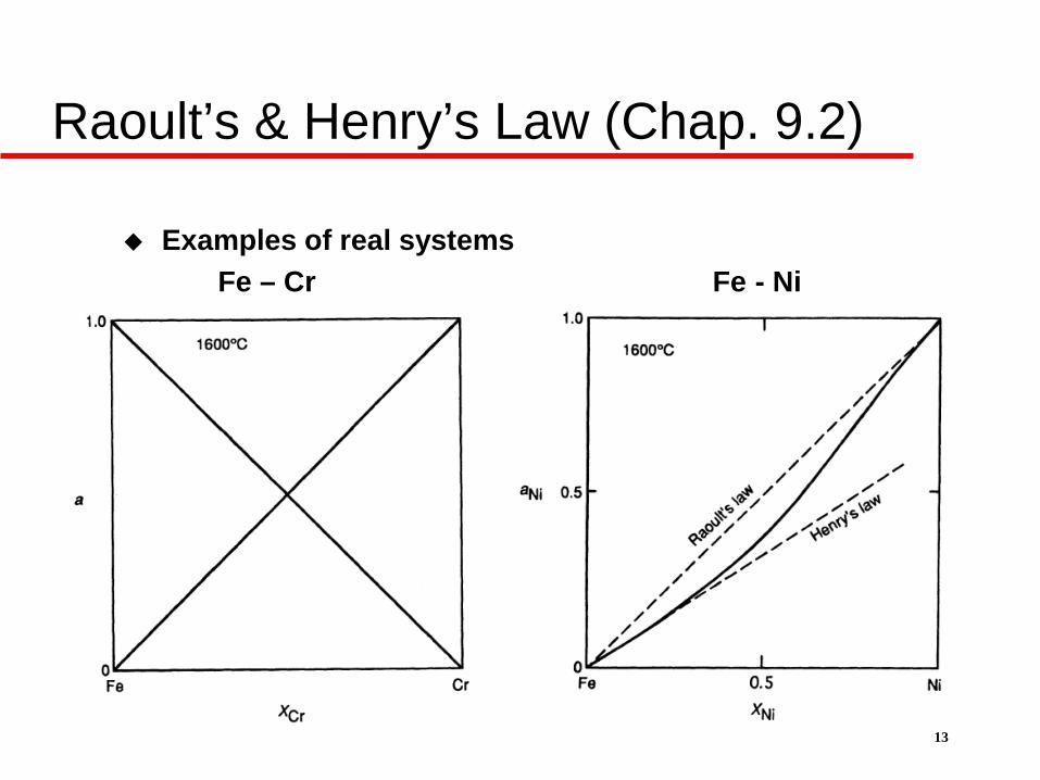
Raoult’s & Henry’s Law (Chap. 9.2)

Examples of real systemsFe – Cr Fe - Ni

13

Raoult’s & Henry’s Law (Chap. 9.2)

Fe - Si

14

Activity of a Component in Solution (Chap. 9.3)

Thermodynamic activity of a component in any state at the temperature is defined as the ratio of fugacity of the component to the fugacity in the standard state:

In this course, we will assume gases are ideal (fi = pi)

This is the definition of activity (important)– Activity is a ratio (dimensionless)– Standard state is a matter of choice, but you must be

consistent if you are using data– Here the pure liquid is the obvious choice for standard state

15

Activity of a Component in Solution (Chap. 9.3)

If the solution follows Raoult’s Law, then

This is also Raoult’s Law, But remember Raoult’s

Law is based on vapour pressures

16

Activity of a Component in Solution (Chap. 9.3)

In the range that Henry’s Law applies there is also a linear behaviour:

Again, this is a simple way to state Henry’s Law, but is related to vapour pressures

17

Activity of a Component in Solution (Chap. 9.3)

By the definition of activity, the activity of the component is 1 when it is in its standard state

For Raoult’s Law this is straightforward because – ai = 1 when Xi = 1

For Henry’s Law

– ai = 1 when Xi = 1/ki, so this is a different standard state– For Ni k is approximately 0.6, so the standard state of Ni is a

mole fraction of 1.67 which cannot exist in nature– Clearly, we are extrapolating Henry’s Law beyond its

applicability in this case This shows we pick our standard states for convenience, so

be careful18

The Gibbs-Duhem Equation (Chap. 9.4)

We must rely on some thermodynamic measurement of activity– Direct measurement of vapour pressure of a component– Electro-chemical measurements (Chap. 15, Mtls 3C03)

Often in these measurements only 1 component can be measured

We obtain the other one with the Gibbs-Duhem Equation The derivation is for a general extensive thermodynamic

property, Q, but when people speak of the Gibbs-Duhem Equation, it refers to the case of G as Q

The (eventual) aim of this derivation is to relate the change of the activity of component 1 to the activity of component 2

19

The Gibbs-Duhem Equation (Chap. 9.4)

Any extensive property is a function of T, P and the number of moles of the solution

At constant T and P, changes in Q are:

The partial molar value of the extensive property is:

More compactly the second last equation is:

20

The Gibbs-Duhem Equation (Chap. 9.4)

Q’ is made up of the partial values times the number of moles of each component

Differentiating with respect to all terms gives:

Noting on the last page

Subtracting the 2 equations gives:

Or generally:

Dividing by the total number of moles21

The Gibbs Free Energy of Formation of a Solution (Chap. 9.5)

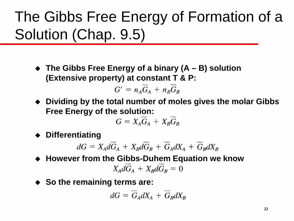
The Gibbs Free Energy of a binary (A – B) solution (Extensive property) at constant T & P:

Dividing by the total number of moles gives the molar Gibbs Free Energy of the solution:

Differentiating

However from the Gibbs-Duhem Equation we know

So the remaining terms are:

22

The Gibbs Free Energy of Formation of a Solution (Chap. 9.5)

From the previous page:

For the binary solution

This conveniently gives:

Multiplying by XB gives:

Adding

Gives:23

The Gibbs Free Energy of Formation of a Solution (Chap. 9.5)

Relationship between the partial molar Gibbs Free Energies and the Molar Gibbs Free Energy of the Solution

These relationships will be used in the Tangential Intercept Method later

24

The Gibbs Free Energy of Formation of a Solution (Chap. 9.5)

Pure component i has a vapour pressure of poi

Component i in solution has a vapour pressure of pi

Recall that the Gibbs free energy change at constant temperature in a closed system is:

We are trying to find what is the difference in Gibbs Free Energy in the solution compared to the pure state

The difference in the state is the difference in pressure in the vapour because the solution and vapour are in equilibrium (ignore the (b) subscript)

25

The Gibbs Free Energy of Formation of a Solution (Chap. 9.5)

The pressure ratio is defined as the activity, so the Gibbs free energy change in going from the pure i to i in solution is:

This change is called the partial molar Gibbs free energy of the solution of i (important)

Also called the partial molar Gibbs free energy of mixing Note that this is not an absolute quantity; it is defined in

terms of a difference between the solution and the standard state (taken to the pure i)

This is the same way we defined activity The superscript o means standard state

26

The Gibbs Free Energy of Formation of a Solution (Chap. 9.5)

So far we have the partial molar Gibbs Free Energy for i Let’s look at the free energy change for the whole solution,

taking a binary A – B solution (constant T & P)

The change is:

Using the definition of the partial Free Energy of Mixing:

27

The Gibbs Free Energy of Formation of a Solution (Chap. 9.5)

Simple expression for the molar Gibbs Free Energy change for the making the mixture or solution (important):

This quantity is plotted here

Note that it depends on measured activities which come from solution vapour pressure

28

Chap. 9.5

Method of Tangential Intercepts (important)

From the Gibbs-Duhem Equation:

29

Partial molar values are obtainedby the tangential intercepts

at XA = 1 and XB = 1

Properties of Raoultian Ideal Solutions (Chap. 9.6)

Recall that the Raoultian solution is one in which A and B have no preference for A or B, almost identical

From Chapter 8, the general state properties are applicable:– For the solution

– For the pure component i

30

Properties of Raoultian Ideal Solutions (Chap. 9.6)

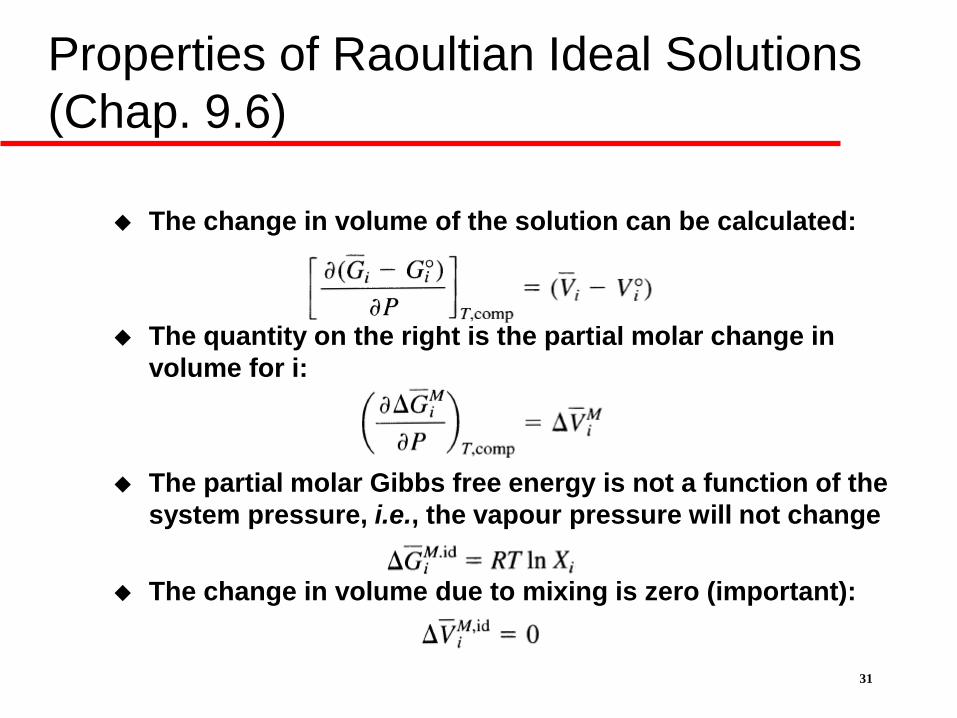
The change in volume of the solution can be calculated:

The quantity on the right is the partial molar change in volume for i:

The partial molar Gibbs free energy is not a function of the system pressure, i.e., the vapour pressure will not change

The change in volume due to mixing is zero (important):

31

Properties of Raoultian Ideal Solutions (Chap. 9.6)

Change in volume due to mixing

Linear change Tangents trivial Makes sense because A

and B do not have any interaction, but they do have different molar volumes

32

Properties of Raoultian Ideal Solutions (Chap. 9.6)

The heat of formation can be derived in a similar way, starting with the Gibbs-Helmholtz equation:– For the solution

– For the pure component

The different due to the mixing process is:

33

Properties of Raoultian Ideal Solutions (Chap. 9.6)

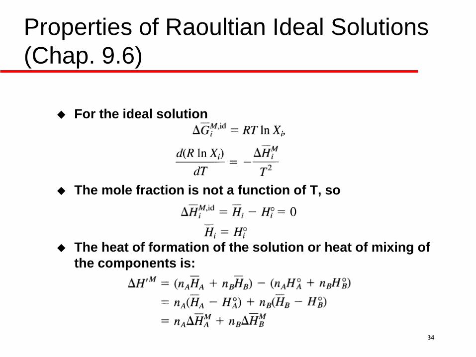
For the ideal solution

The mole fraction is not a function of T, so

The heat of formation of the solution or heat of mixing of the components is:

34

Properties of Raoultian Ideal Solutions (Chap. 9.6)

The heat of mixing of an ideal solution is zero Again this makes sense because there are no particular

interactions between A and B that are different from between A and A and B and B

The volume change of an ideal solution is zero Now we will look at the entropy of mixing of an ideal

solution; it is NOT zero– In the mixing process we are increasing the randomness of the

components– Mixing is a spontaneous process because we are increasing

the entropy (even with no heat or volume changes)– “Unmixing”, the reverse process is impossible, without a

process or device to do something like distillation, refining or other chemical process

35

Properties of Raoultian Ideal Solutions (Chap. 9.6)

Previous relationship (Eq. 5.25)

This also applies for the formation of a solution:

We previously derived for an ideal solution:

So the entropy change for forming an ideal solution is:

36

Properties of Raoultian Ideal Solutions (Chap. 9.6)

Entropy of formation of an ideal solution is independent of temperature

Entropy of formation is always positive (spontaneous) Heat of formation is zero, so the only contribution to the

Gibbs free energy of formation is due to entropy Statistical thermodynamic derivation to show that the

entropy of mixing is the configurational entropy (entropy which arises from the number of ways in which the energy of the system can be shared by the atoms)

37