The Beginning of a Beautiful Friendship:

The Impact of Hiring-Cohort Connections on Job Referral∗ †

Ayal Chen-Zion¶

UC San Diego

April 15, 2016

Abstract

Connections with former co-workers are important for labor mobility. Co-workers that werehired at the same time, the hiring-cohort, enter an existing work landscape together. I find thatthey serve as unique sources of job referral later in life. A simple model of relationship for-mation from Chen-Zion and Rauch (2016) predicts a tendency for connections to persist overtime. This theory implies that a worker’s hiring-cohort co-workers are an important source ofemployment opportunities because they are more likely to have a pre-existing working rela-tionship. I am able to study how hiring-cohort co-workers influence where a displaced workeris hired by using a Brazilian employee-employer dataset. The existence of hiring-cohort co-workers and the quantity of former co-workers at a plant have a significant positive effect onthe probability of acquiring a job at that plant, following unemployment. The existence ofone hiring-cohort co-worker increases the chance of going to a plant by 3.7-fold which is 2.75times more than one non-hiring-cohort co-worker. I also address several biases associatedwith inferred job referral in the existing literature and show that results are robust to placebotests and controlling for selection on unobservable characteristics (with a peers-of-peers in-strument).Keywords: labor; employment; job referral; hiring-cohorts; social networks; firm closureJEL Classification: J63,J64,J65

∗Thanks to James Rauch for the advice and guidance throughout the entire process of writing this paper and toMarc Muendler for meaningful comments and for granting access to the RAIS data. Additional thanks to NageebAli, Gordon Dahl, Kevin Lewis, Mark Jacobson, Laura Gee, Joey Engelberg, Mitch Downey, Jeffrey Shrader, LelandFarmer and Michael Levere for many helpful comments. I would also like to thank the attendants of the UCSDApplied Lunch and Seminar for their insights. The author is responsible for any errors.†The latest version can be found on my website.¶achenzio@ucsd.edu (achenzion.github.io).

1

Contents1 Introduction 3

2 Literature 5

3 Data: Brazilian Work Histories 63.1 Displaced Workers . . . . . . . . . . . . . . . . . . . . . . . . . . . . . . . . . . 83.2 Historic co-workers . . . . . . . . . . . . . . . . . . . . . . . . . . . . . . . . . . 93.3 Summary Statistics . . . . . . . . . . . . . . . . . . . . . . . . . . . . . . . . . . 11

4 Results: Impact of a Historic Co-worker on Job Referral 15

5 Hiring-Cohort: Relationships with some co-workers are more likely than others 215.1 Theory of Hiring-Cohort Attachment . . . . . . . . . . . . . . . . . . . . . . . . . 215.2 Results . . . . . . . . . . . . . . . . . . . . . . . . . . . . . . . . . . . . . . . . . 22

6 Robustness to Alternative Explanations 246.1 Placebo Histories . . . . . . . . . . . . . . . . . . . . . . . . . . . . . . . . . . . 246.2 Placebo Potential Plants . . . . . . . . . . . . . . . . . . . . . . . . . . . . . . . . 266.3 Alter Characteristics . . . . . . . . . . . . . . . . . . . . . . . . . . . . . . . . . 276.4 Instrument for Alters’ Location . . . . . . . . . . . . . . . . . . . . . . . . . . . . 29

7 Conclusion 35

Appendices 40

A Sample Selection 40

B Alter Characteristics 41

C Summary Statistics for Robustness Checks 42

D IV Related Results 47

E Maps 48

2

1 Introduction

A burgeoning industry of firms seek to help job seekers leverage their contacts into a new job. For

example, LinkedIn is improving its Recruiter and Referral products to streamline this process (Lun-

den 2015). Additionally, firms and policy makers must understand which connections provide the

greatest returns to best help their customers and constituents obtain a job at a specific employer. To

this end, this paper focuses on job referral among co-workers, because of their established working

relationship, and determines how they influence referral destination. The co-workers of particular

interest are those who started at the same time at previous jobs - hiring-cohort co-workers. The

hiring-cohort is comprised of co-workers from a range of ages, industries and occupations, but the

common bond that leads to a connection comes from having to navigate a new environment at the

same time. By “going through the fire” together, the hiring-cohort co-workers are shown to be

more likely to develop an initial relationship and with persistence in interaction this relationship

leads to a more useful referral source for a specific employer in the future. This prediction is vali-

dated in the data and suggests that not all co-workers are equally likely to serve as referral sources,

even conditional on characteristics. The focus on the hiring-cohort is the main contribution of

this paper and has been missing from the previous research discussion of job referral. An addi-

tional contribution of this paper is a careful treatment of inferring job referral from job histories

and start/end dates. The literature has overstated the connection effect by not accounting for the

compatibility of the worker and firm.

Previous research has studied the impact of neighbors, friends and family on employment

(Bayer, Ross, and Topa 2008, Kramarz and Skans 2014, Schmutte 2015, Nordman and Pasquier-

Doumer 2015, Gee, Jones, and Burke forthcoming). Co-workers are of particular interest in labor

mobility because their shared experience provides highly relevant information on a job seeker’s

productivity (Granovetter 1995, Cingano and Rosolia 2012, Muendler and Rauch 2015, Chen-

Zion and Rauch 2016). Recent papers, discussed in Section 2, focus on former co-workers as

connections for a job referral and study the impact on employment destination and post-referral

outcomes (Saygin, Weber, and Weynandt 2014, Hensvik and Skans forthcoming, Brown, Setren,

and Topa 2016). In the literature, job referral refers to (a) a worker obtaining any job because of

information obtained through connections or (b) a worker obtaining a job at a firm where a referrer

is employed. This paper focuses on the latter.

I study how the probability that a displaced worker obtains a job at a particular employer is

3

influenced by a former co-worker being employed there - a connection. Consider two workers

who just entered the job market following the same firm closure. They can both potentially go to

work at an employer, the first worker used to work with an employee of the potential employer,

while the second worker does not know anyone at the potential employer. Assuming that they are

identical apart from their connection, the impact of a connection is the increase in likelihood that

the connected worker goes to the potential employer relative to the worker with no connection.

Multiple job seekers displaced from the same firm closure have differences in connection to a

potential employer and thus provide identifying variation for estimation of a connection effect at a

worker-potential employer level. Previous work overstates the importance of connections because

it does not accurately account for alternative reasons the worker would start at a potential employer.

A methodological contribution of this paper is to more rigorously account for these alternatives.

Beyond a more careful treatment of referral, I find that those potential employers with a hiring-

cohort co-worker are more likely to be destinations of a job seeker. Theory predicts that the differ-

ence in effect is due to hiring-cohort co-workers being more likely than others to have developed

a relationship which then persists until the worker needs to look for a job (Chen-Zion and Rauch

2016). Additionally, the hiring-cohort connections may form a special type of relationship. It is

important to note that the literature has studied differences in referral by type of relationship, but

tends to focus on characteristics of the agents on either side, like age, or very different types of

relationships, like familial versus former co-workers. This is one of the first papers to focus on

the characteristics and likelihood of the relationship within a type (former co-workers), namely the

difference between co-workers in the hiring-cohort versus those that entered at other times.

Section 3 discusses the Brazilian employee-employer dataset, Relacao Anual de Informacoes

Sociais (RAIS), that is used to define co-workers and trace labor mobility. Section 4 uses a regres-

sion framework at a worker-potential employer level to benchmark the results in Brazil against the

literature. It improves on previous specifications by restricting the set of co-workers and control-

ling for compatibility between the worker and potential hiring employer. This paper then diverges

from the previous literature to explore the impact of the number of co-workers at the potential

hiring employer.

Next, Section 5.1 reviews the results of Chen-Zion and Rauch (2016) regarding the importance

of hiring-cohort co-workers in network formation. Section 5.2 returns to a regression framework

and establishes the existence of a significant hiring-cohort co-worker effect. The existence of one

4

hiring-cohort co-worker increases the chance of being hired at a specific plant by 3.7-fold which is

2.75 times more than one non-hiring-cohort co-worker.

The results are extended in Section 6 to show that they are robust to multiple identification

threats by using placebo sets of former co-workers and potential employers, controlling for alter

characteristics and constructing a peers-of-peers instrument.

2 Literature

As highlighted in a review article by Ioannides and Loury (2004), the academic study of job referral

dates back to Granovetter (1973, 1983, 1995, 2005) and Rees (1966). In his book, “Getting a Job:

A Study of Contacts and Careers”, Granovetter interviews 282 professional, technical and man-

agerial working men from Newton, Massachusetts with employer changes. 55.7% of his sample

use personal connections to find a job, 68.7% of which used a person known from a work environ-

ment. These results have been found to be stable and have given rise to an expansive literature on

the role of social connections in the labor market. The introduction of large employee-employer

datasets and advanced computational techniques have allowed researchers to move beyond small

case studies to create a more detailed picture of the relationship between labor mobility and job

referral.

One strand of this literature studies the employment outcomes, like wage and tenure, by looking

at outcomes for referred, non-referred and referring employees (Hensvik and Skans forthcoming,

Pallais and Sands forthcoming). Pallais and Sands (forthcoming) find gains in candidate quality

from referral, importantly they find referrer-referee teams perform better than other pairings. This

is consistent with the theory developed in Chen-Zion and Rauch (2016) where worker specific

match quality are a major driver of referrals. To test this model further, in this paper I contribute

to a complimentary literature on the inputs into a job referral and how connections influence the

acquisition of a referral at a specific employer. For example, Saygin, Weber, and Weynandt (2014)

use Austrian employee-employer data to study how an individual’s network changes his/her re-

employment probability and how having a former co-worker at a specific firm impacts the prob-

ability of obtaining a job. They find that being connected to a firm by a historic co-worker more

than doubles the chances that the worker is hired. This finding provides a benchmark for this study

of the impact of a connection on referral to a specific employer.

5

The theoretical literature behind job referral has focused on post-referral outcomes, but of equal

importance is the process by which a job seeker receives a referral. Recent evidence supports an

important role of learning and a desire to work together as post-referral motivators for referral

(Pallais and Sands forthcoming, Brown, Setren, and Topa 2016). Chen-Zion and Rauch (2016)

develop a model of pre-referral relationship formation to help understand which co-workers an

employee would like to work with, it is with this in mind that I turn to the hiring-cohort. The hiring-

cohort has been missing from the job referral literature, but the importance of the hiring-cohort in

co-worker interaction has been recognized in the sociology literature; hiring-cohort connections

naturally occur because of the difficulty of “penetrating established communication networks”

(Zenger and Lawrence 1989). Zenger and Lawrence (1989) find high rates of communication

between cohort members across teams. This highlights the fact that the hiring-cohort serves as an

observable proxy for a higher likelihood of a relationship in a dataset where individual interaction

cannot be observed. The initial connection between cohort members couples with persistence in

interaction to yield greater interaction at a later date, or cohort attachment. Chen-Zion and Rauch

(2016) formalizes this mechanism and show that it is evident in the major decision of who an

entrepreneur brings with him to a spinoff firm. This tendency for a cohort connection to influence

the employment path is not inherently unique to entrepreneurship. Section 5.1 goes over the main

components and extensions necessary to study cohort attachment in the job referral context.

3 Data: Brazilian Work Histories

This paper’s empirical analysis of job referral uses the Relacao Anual de

Informacoes Sociais (RAIS), an annual administrative census of the Brazilian formal sector labor

force conducted by the Ministry of Labor (Ministerio de Trabalho, MTE).1 This paper uses the data

from 1994 to 2001. The dataset extends back to 1986, but important variables are missing prior

to 1994 so those years are not used in the analysis.2 Submission of this information is enforced

by Brazilian law, under threat of fines. Allocation of workers’ government benefits is based upon

these records and so there is incentive for workers and firms to report.

1This dataset is used under an agreement organized by Marc Muendler, mmuendler@ucsd.edu. Other papers thathave used these data include Menezes-Filho, Muendler, and Ramey (2008), Muendler, Rauch, and Tocoian (2012),Muendler and Rauch (2015) and Chen-Zion and Rauch (2016).

2Additionally, access to data from 2002-2009 has recently been obtained and will be added in future work. Varia-tion in job referral over time is beyond the scope of this paper, but is studied in-depth by Galenianos (2014).

6

The use of an employee-employer dataset provides the distinct advantage of being able to track

workers through their job histories and not rely of survey data to construct the set of connections.

This can be done because the dataset includes unique identifiers for workers and plants within

a firm3 that can be tracked across time, as well as information on the workers’ demographics,

occupation4 , industry, location and month of hiring/leaving.

MTE estimates that roughly 90% of Brazilian employees in the formal sector are covered in

RAIS (Muendler, Rauch, and Tocoian 2012). RAIS does not include the large Brazilian informal

sector which constitutes approximately 50% of the population (Henley, Arabsheibani, and Carneiro

2009). Unemployment in this dataset is unemployment+informal employment. Formal sector em-

ployment is considered preferable to informal employment because of the large benefits that are

awarded based on RAIS reporting. For a more extensive discussion of the choice between the

formal and informal sector in Brazil see Menezes-Filho, Muendler, and Ramey (2008), Bosch and

Maloney (2010), Bosch and Esteban-Pretel (2012).

I take a number of steps to arrive at a dataset for which the results are meaningful and com-

parable to other studies of former co-workers and job referral. The universe of employment is

restricted to males,5 working more than 20 hours per week, in job spells lasting more than three

months. This rules out transitory employment where workers work at the same plant with a low

probability of actually communicating, such as part-time or short-term labor.

The data only includes five of Brazil’s 26 states,6 Ceara, Acre, Santa Catarina, Mato Grosso do

Sul, and Espirito Santo. These five states were chosen because they represent different geographic

(see Figure E.1) and demographic circumstances in Brazil. Estimates are pooled across states

with each state considered in isolation, so obtaining a job outside of the state is not considered.

This is justified primarily by computational concerns regarding the time and resources necessary

3The plant is the establishment of interest for relationships because that is the level at which relationships are mostlikely to be formed. The only exception in this paper is that closure is considered at the firm level (see Section 3.1 for amore detailed discussion). Most results generalize to using the firm, but some robustness checks cannot be conductedat that level and so those results are not currently reported in the paper. Firm-level results are available upon requestfrom the author.

4RAIS has job titles that are matched to three digit group identifier in Brazil’s standard occupation classificationsystem Classificacao Brasileira de Ocupacoes (CBO). This paper uses the 1994 CBO system. For more informationon the CBO and its relation to international classification systems see Muendler, Poole, Ramey, and Wajnberg (2004).

5Bosch and Maloney (2010) use another Brazilian dataset that measures informal employment, Pesquisa Mensualdo Emprego (PME), and suggest that transition probabilities between the formal sector, informal sector and unem-ployment are considerably different between men and women.

6For maps on geographic location, population distribution and migration see Appendix E.

7

to track and compare job histories among workers.7 Figure E.3 shows that there is substantial

migration in Brazil in 2000, but at relatively low levels in the chosen states. Additionally, the issue

of migration is also present in previous results from other countries and so does not take away

from the comparison. The states used had total populations of 8.4, 0.7, 6.2, 2.4, and 3.5 million,

respectively, in 2010, with corresponding densities of 56.76 , 4.47, 65.27, 6.86, and 76.25 per km2

(IBGE 2010)8. Similar projects have used employee-employer datasets from European countries

like Sweden and Austria (Hensvik and Skans forthcoming, Saygin, Weber, and Weynandt 2014),

which have comparable populations (densities) of 9.4 (23) and 8.4 (102) million (per km2) in 2010,

respectively (World Bank WDI 2014). This is the first paper to conduct this type of analysis outside

of Europe. Given the differences, the consistency of the results with previous studies emphasizes

their robustness. Future work may extend this analysis to the entirety of Brazil.

3.1 Displaced Workers

Within the universe of workers, the workers of interest are individuals who enter a new job fol-

lowing unemployment from firm closure. Firm closure occurs in year t if the firm last appears in

the data in year t. I do not include individual plant closures because they can represent consolida-

tion by the employer and that would overstate the result. Closures represent plausibly exogenous

unemployment and prevent issues of selection into job transition with the added benefit of provid-

ing a natural set of comparison workers. There is concern that the closure is not exogenous. The

solution is to include all workers who were at the closure firm in the last year it appeared in the

data, as suggested by Schwerdt (2011). To avoid including small firms that are slowly failing I

also require that at least five employees work at the closure in its last year. To address concerns

that co-workers from the closure firm select into leaving prior to closure, I restrict connections to

co-workers from employment prior to working at the closing firm. This is the first main departure

from the previous literature which also includes co-workers from the closure job spell (see Section

4 for more information). The sample includes closures from 1998-1999 to allow for a minimum

of four years (1994-1998) of work history and two years (2001-1999) to obtain another job. For

consistency across workers, I only consider four years of work history prior to the month they left

7In terms of complexity, matching workers to co-workers is an O(n2) task. This reason is particularly exacerbatedwhen tracking workers for the peers-of-peers instrument that requires tracking the co-workers of former co-workers,an O(n3) task.

8The Brazilian statistical bureau, Instituto Brasilero de Geografia e Estatıstica. http://www.ibge.gov.br

8

the closure and the first job acquired within two years of leaving the closure. This is similar to the

selection procedure in Saygin, Weber, and Weynandt (2014), but they use five years prior and one

year after because of a larger panel and greater re-employment rate (possibly because of the lack

of a large Austrian informal sector). Each worker leaving a closure is referred to as an ego. This

terminology is from the sociology literature on networks with a specific individual of interest for

the purpose of outcomes and other individuals for the purpose of covariates. These are often called

egocentric networks (Marsden 1990). If an ego is at multiple closures then I only use his observa-

tion at the last closure observed in the data. Additionally, if the ego leaves the closure because of

death or retirement they are excluded from the sample.

3.2 Historic co-workers

The next important component is the set of co-workers. The first step is to trace the ego back to

all plants in his employment history, prior to his employment at the closure firm9. Co-workers are

those who were at the same plant at the same time and are referred to as alters. I restrict connections

to those where the ego and alter overlap for more than three months to minimize measurement error

of the underlying relationship. The set of alters for a given ego are the ego’s connections. Those

alters at a specific plant when the ego becomes unemployed are the ego’s connection to the plant.

I require that the alter is at the plant at least three months before the closure in order to assure

that contemporaneous movement effects do not exist. For the purposes of this paper, those plants

where an alter is employed at the time of closure are termed the alter-plants of a specific ego. As

noted before, plants are considered for relationship formation and referral, while firms (possibly

with multiple plants) are considered for closure. Less than 6% of firms have more than two plants

in any given year. Within the set of alters, the subset that are hiring-cohort co-workers, or cohort-

alters, started +/− 2 months from the ego at the historic plant at which they first worked together.

This is done because our universe of employment spells is restricted to those lasting more than

three months and so it implies that there is a minimum of one month overlap between the ego and

alter.

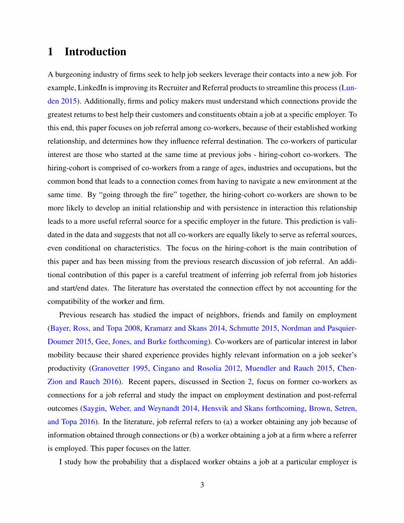
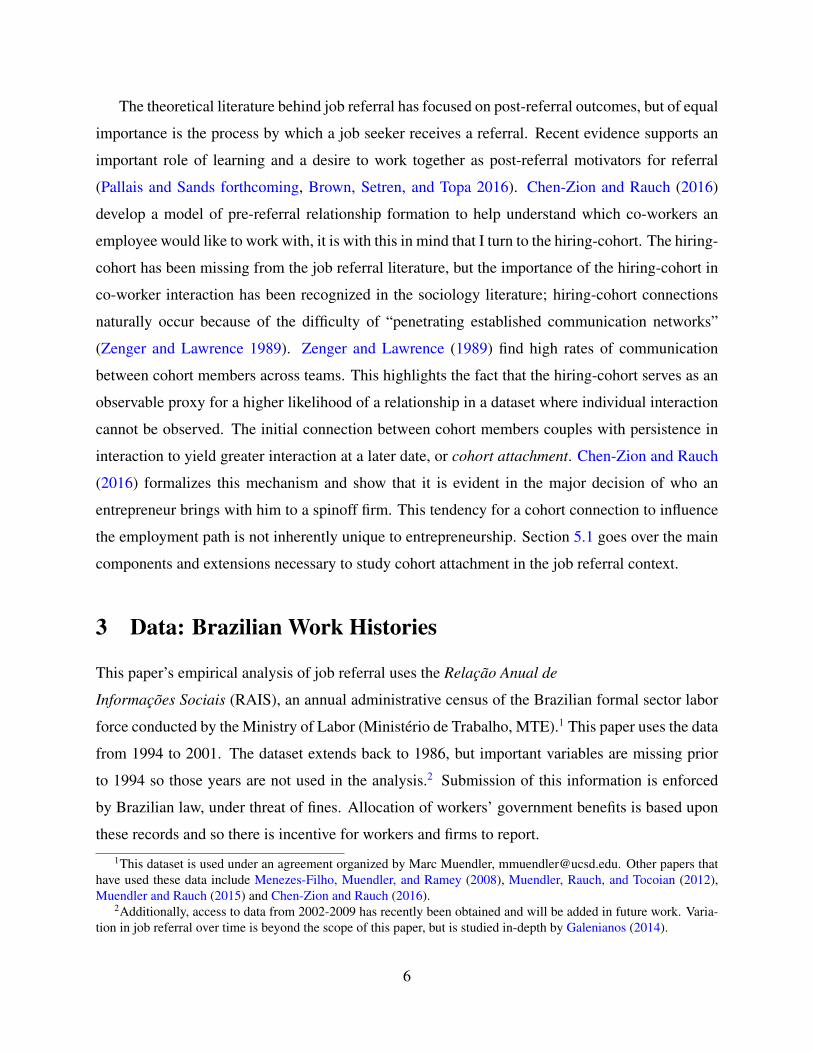
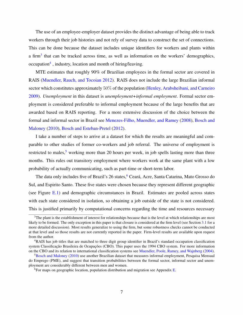
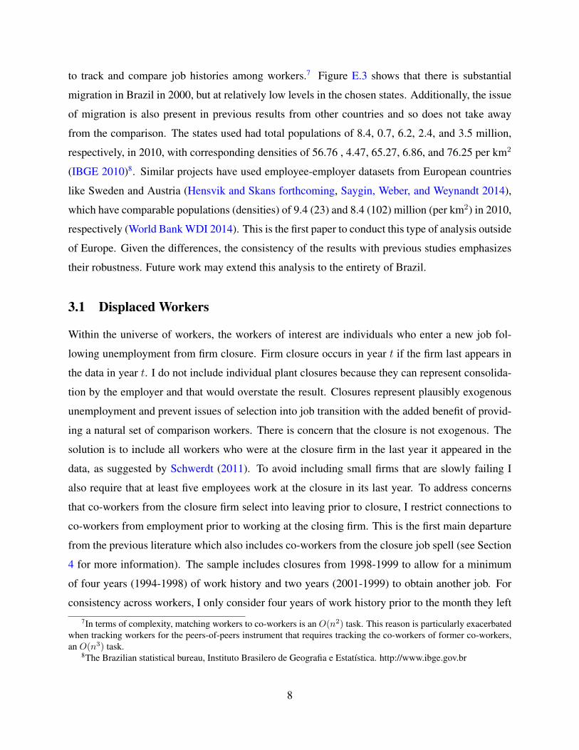
Figure 1 depicts the simple case of one closure with two egos. The “treatment” ego has one

historic plant and met one alter. At the time of the closure the alter is at a potential hiring plant.

9This is true for all but the first column in Table 4 where closure co-workers are included if they are not also egos.See Section 4 for a discussion of how this differs from the previous literature.

9

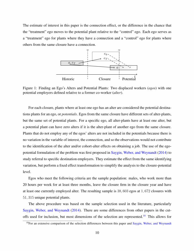
The estimate of interest in this paper is the connection effect, or the difference in the chance that

the “treatment” ego moves to the potential plant relative to the “control” ego. Each ego serves as

a “treatment” ego for plants where they have a connection and a “control” ego for plants where

others from the same closure have a connection.

Historic Closure Potentialt

a, eT

e0eT

a

Figure 1: Finding an Ego’s Alters and Potential Plants: Two displaced workers (egos) with onepotential employers defined relative to a former co-worker (alter).

For each closure, plants where at least one ego has an alter are considered the potential destina-

tions plants for an ego, or potentials. Egos from the same closure have different sets of alter-plants,

but the same set of potential plants. For a specific ego, all alter-plants have at least one alter, but

a potential plant can have zero alters if it is the alter-plant of another ego from the same closure.

Plants that do not employ any of the egos’ alters are not included in the potentials because there is

no variation in the variable of interest, the connection, and so the observations would not contribute

to the identification of the alter and/or cohort-alter effects on obtaining a job. The use of the ego-

potential formulation of the problem was first proposed in Saygin, Weber, and Weynandt (2014) to

study referral to specific destination employers. They estimate the effect from the same identifying

variation, but perform a fixed effect transformation to simplify the analysis to the closure-potential

level.

Egos who meet the following criteria are the sample population: males, who work more than

20 hours per week for at least three months, leave the closure firm in the closure year and have

at least one currently employed alter. The resulting sample is 38, 603 egos at 1, 672 closures with

51, 315 unique potential plants.

The above procedure was based on the sample selection used in the literature, particularly

Saygin, Weber, and Weynandt (2014). There are some differences from other papers in the cut-

offs used for inclusion, but most dimensions of the selection are represented.10 This allows for10For an extensive comparison of the selection differences between this paper and Saygin, Weber, and Weynandt

10

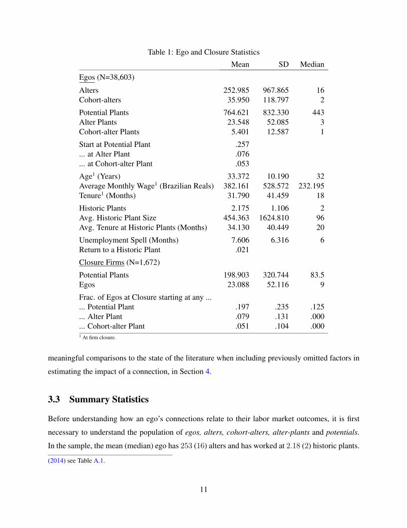
Table 1: Ego and Closure Statistics

Mean SD Median

Egos (N=38,603)

Alters 252.985 967.865 16Cohort-alters 35.950 118.797 2

Potential Plants 764.621 832.330 443Alter Plants 23.548 52.085 3Cohort-alter Plants 5.401 12.587 1

Start at Potential Plant .257... at Alter Plant .076... at Cohort-alter Plant .053

Age1 (Years) 33.372 10.190 32Average Monthly Wage1 (Brazilian Reals) 382.161 528.572 232.195Tenure1 (Months) 31.790 41.459 18

Historic Plants 2.175 1.106 2Avg. Historic Plant Size 454.363 1624.810 96Avg. Tenure at Historic Plants (Months) 34.130 40.449 20

Unemployment Spell (Months) 7.606 6.316 6Return to a Historic Plant .021

Closure Firms (N=1,672)

Potential Plants 198.903 320.744 83.5Egos 23.088 52.116 9

Frac. of Egos at Closure starting at any ...... Potential Plant .197 .235 .125... Alter Plant .079 .131 .000... Cohort-alter Plant .051 .104 .0001 At firm closure.

meaningful comparisons to the state of the literature when including previously omitted factors in

estimating the impact of a connection, in Section 4.

3.3 Summary Statistics

Before understanding how an ego’s connections relate to their labor market outcomes, it is first

necessary to understand the population of egos, alters, cohort-alters, alter-plants and potentials.

In the sample, the mean (median) ego has 253 (16) alters and has worked at 2.18 (2) historic plants.

(2014) see Table A.1.

11

These egos are located at 1, 672 closure firms with each closure having a mean (median) of 23.1

(9) egos and 198.9 (83.5) potential plants (see Table 1).

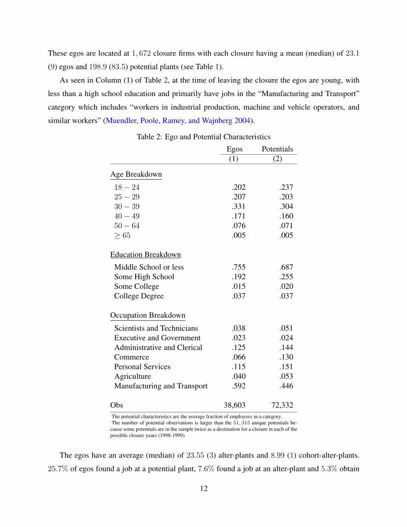
As seen in Column (1) of Table 2, at the time of leaving the closure the egos are young, with

less than a high school education and primarily have jobs in the “Manufacturing and Transport”

category which includes “workers in industrial production, machine and vehicle operators, and

similar workers” (Muendler, Poole, Ramey, and Wajnberg 2004).

Table 2: Ego and Potential Characteristics

Egos Potentials(1) (2)

Age Breakdown

18− 24 .202 .23725− 29 .207 .20330− 39 .331 .30440− 49 .171 .16050− 64 .076 .071≥ 65 .005 .005

Education Breakdown

Middle School or less .755 .687Some High School .192 .255Some College .015 .020College Degree .037 .037

Occupation Breakdown

Scientists and Technicians .038 .051Executive and Government .023 .024Administrative and Clerical .125 .144Commerce .066 .130Personal Services .115 .151Agriculture .040 .053Manufacturing and Transport .592 .446

Obs 38,603 72,332The potential characteristics are the average fraction of employees in a category.The number of potential observations is larger than the 51, 315 unique potentials be-

cause some potentials are in the sample twice as a destination for a closure in each of thepossible closure years (1998-1999)

The egos have an average (median) of 23.55 (3) alter-plants and 8.99 (1) cohort-alter-plants.

25.7% of egos found a job at a potential plant, 7.6% found a job at an alter-plant and 5.3% obtain

12

a job at a cohort-alter-plant. Within the closures the average (median) fraction of egos obtaining a

job at a potential plant is 19.7% (12.5%) with 7.9% (0%) obtaining a job at an alter-plant and 5.1%

(0%) at a cohort-alter-plant

Of the 51, 315 unique potentials there are 72, 332 potential × year observations because some

are potentials for closures in multiple years (1998-99). Column (2) of Table 2 presents the mean

fraction of employees at the potential in the closure year with a given characteristic. For example,

on average 23.7% of each potential is between 18 and 24 years old. The distribution of ages,

education and occupation within a potential is similar to that in the ego population. Understanding

how the ego compares to the potential plant is important because any similarity can confound the

ego’s tendency to go to the plant, beyond the referral mechanism. This feature has been largely

overlooked and as shown in Section 4, it is crucial to an unbiased estimate of the connection effect.

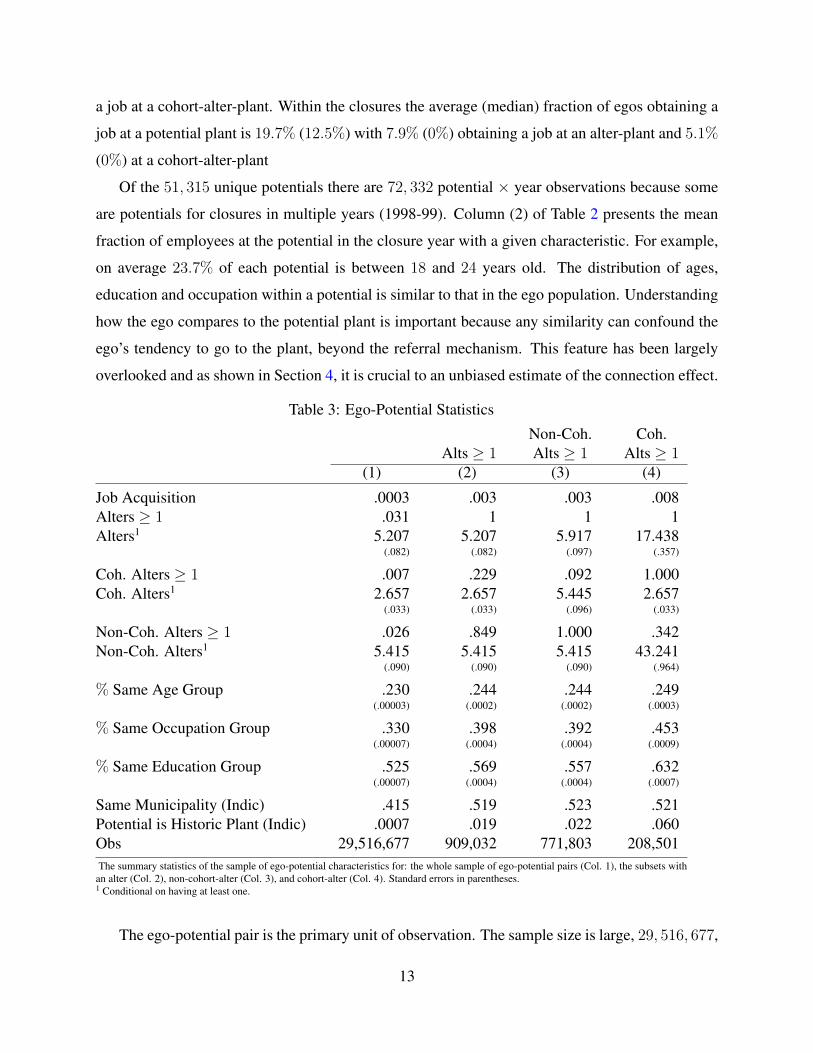
Table 3: Ego-Potential Statistics

Non-Coh. Coh.Alts ≥ 1 Alts ≥ 1 Alts ≥ 1

(1) (2) (3) (4)

Job Acquisition .0003 .003 .003 .008Alters ≥ 1 .031 1 1 1Alters1 5.207 5.207 5.917 17.438

(.082) (.082) (.097) (.357)

Coh. Alters ≥ 1 .007 .229 .092 1.000Coh. Alters1 2.657 2.657 5.445 2.657

(.033) (.033) (.096) (.033)

Non-Coh. Alters ≥ 1 .026 .849 1.000 .342Non-Coh. Alters1 5.415 5.415 5.415 43.241

(.090) (.090) (.090) (.964)

% Same Age Group .230 .244 .244 .249(.00003) (.0002) (.0002) (.0003)

% Same Occupation Group .330 .398 .392 .453(.00007) (.0004) (.0004) (.0009)

% Same Education Group .525 .569 .557 .632(.00007) (.0004) (.0004) (.0007)

Same Municipality (Indic) .415 .519 .523 .521Potential is Historic Plant (Indic) .0007 .019 .022 .060Obs 29,516,677 909,032 771,803 208,501The summary statistics of the sample of ego-potential characteristics for: the whole sample of ego-potential pairs (Col. 1), the subsets with

an alter (Col. 2), non-cohort-alter (Col. 3), and cohort-alter (Col. 4). Standard errors in parentheses.1 Conditional on having at least one.

The ego-potential pair is the primary unit of observation. The sample size is large, 29, 516, 677,

13

because each of the 38, 603 egos is paired with all potential plants from their closure, on average

199, with positive correlation at a closure between the number of egos and potentials. The sample

size for a given closure scales quickly in the number of egos because one additional ego adds

an observation for the new ego with that ego’s alter-plants, all other egos’ alter-plants, and for

other egos with the new ego’s alter-plants. Table 3 summarizes the main variables of interest in

the regression for: the whole sample of ego-potential pairs (Col. 1), subsets with an alter (Col.

2), non-cohort-alter (Col. 3), and cohort-alter (Col. 4). The dependent variable of interest is an

indicator for if an ego obtains a job at the specific potential plant. The mean of this variable, .0003,

can be interpreted as the chance an ego goes to a specific potential plant. 3.1% of ego-potential

pairs have an alter with an average 5.2 alters each, conditional on having at least one. Notice that

the set of potential plants is constructed to contain all plants to which egos are connected, but few

connections exist. The low rate of alter connections is due to different egos from a closure having

divergent job histories and thus different sets of co-workers. Potentials are the union of alter-plants

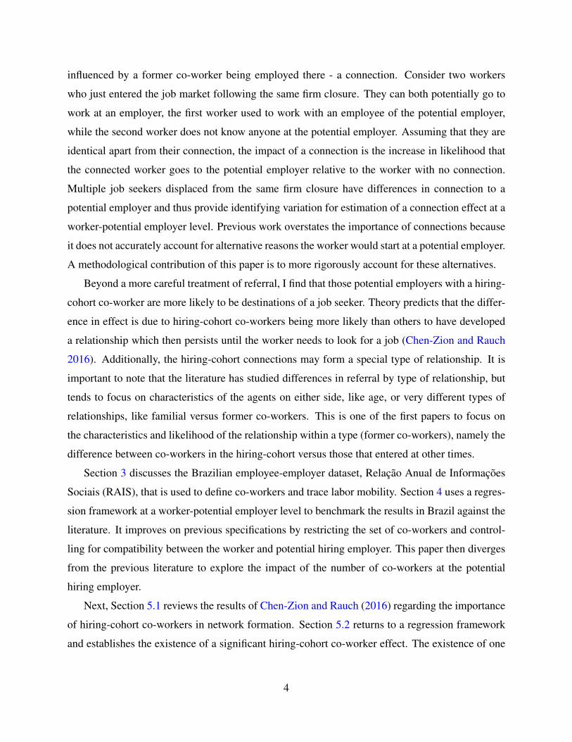
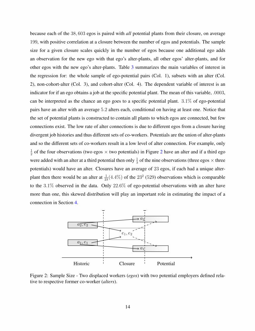
and so the different sets of co-workers result in a low level of alter connection. For example, only12

of the four observations (two egos × two potentials) in Figure 2 have an alter and if a third ego

were added with an alter at a third potential then only 13

of the nine observations (three egos× three

potentials) would have an alter. Closures have an average of 23 egos, if each had a unique alter-

plant then there would be an alter at 123(4.4%) of the 232 (529) observations which is comparable

to the 3.1% observed in the data. Only 22.6% of ego-potential observations with an alter have

more than one, this skewed distribution will play an important role in estimating the impact of a

connection in Section 4.

PotentialClosureHistoric

a1, e1

a2, e2

e1, e2

a1

a2

Figure 2: Sample Size - Two displaced workers (egos) with two potential employers defined rela-tive to respective former co-worker (alters).

14

The compatibility between the ego and potential is a major factor in labor mobility and largely

missed in the previous literature. This bias comes from job referral in large datasets needing to be

inferred from labor mobility. The act of moving to a firm where a connection is employed has stood

as suggestive evidence for referral because the researcher is unable to observe a job referral. I find

this treatment of job referral suspect as there are alternative explanations for mobility that do not

center on referral, such as potential plant demand for a specific set of skills or ego comfort with the

company culture. This is addressed further in Section 4, but for now note that on average 23.0% of a

potential plant’s employees are in the same age group as the ego, 33.0% are in the same occupation

group and 52.5% are in the same education group as the ego.11 Additionally, 41.5% of potentials

are in the same municipality12 as the ego’s location at the closure and 0.07% are also historic

plants of the ego. This last form of ego-potential compatibility is important because returning to a

historic plant is highly correlated with connection to a plant, yet a job acquisition may be unrelated

to referral and actually due to information the ego accessed independently through employment.

Column 2 of Table 3 shows that when conditioning on the existence of an alter connection these

compatibility measures increase. For example, for potentials with an alter 56.9% of the plant’s

employees are in the same education group as the ego. The chance of an ego obtaining a job at

a specific potential also increases to .003 for potentials with an alter. This shows that connection,

compatibility and job acquisition are positively correlated and it is unclear if the increase in the

chance of getting a job at a plant can be attributed to more connection or more compatibility. To

isolate the differential impact of a connection on job referral I move to a regression framework

with the ego-potential pair as the unit of observation so that alternate factors, like compatibility,

can also be addressed.

4 Results: Impact of a Historic Co-worker on Job Referral

The first task is to benchmark results from this setting against the previous literature and address the

omitted variables that have been missed in previous analysis. The central result, the importance of

hiring-cohort co-workers in job referral, does not depend crucially on these factors, but this section

establishes that the effect would be overestimated if not accounting for other factors.11The groups are defined in Table 2.12The municipality is the smallest administrative unit in Brazil. In 2000, Brazil had 5,507 and the five states used

in this analysis had 184 (Ceara), 22 (Acre), 293 (Santa Catarina), 77 (Mato Grosso do Sul), and 77 (Espirito Santo)(IBGE 2000).

15

In the following regression framework, the identification of the impact of a connection is com-

ing from multiple egos, i, from the same closure, c = c(i), who can go to the same potential plant

f . The variation of interest occurs in the existence and type of connection to the potential plant, f .

Recall that i’s alter-plants are a subset of the potentials because i is an ego in c.

The regressions are run with ego-potential plant (if ) observations, but the ego’s connections

are defined on the ego-alter level at a fixed time (when i leaves c(i)). The time dimension is

suppressed because each ego has a unique time that he leaves the closure.

The dependent variable of interest is an indicator for if an ego acquires a job at a potential.

This is a binary outcome, but a linear probability model is used for ease of interpretation.13 This

procedure is similar to that of Saygin, Weber, and Weynandt (2014) and so I first conduct a similar

baseline regression. Saygin, Weber, and Weynandt (2014) use a fixed effect transformation from

Kramarz and Skans (2014) for estimation which reduces the data to closure firm-potential firm

observations. This comes at the cost of being able to address some threats to identification that are

discussed later in this section.

Benchmark

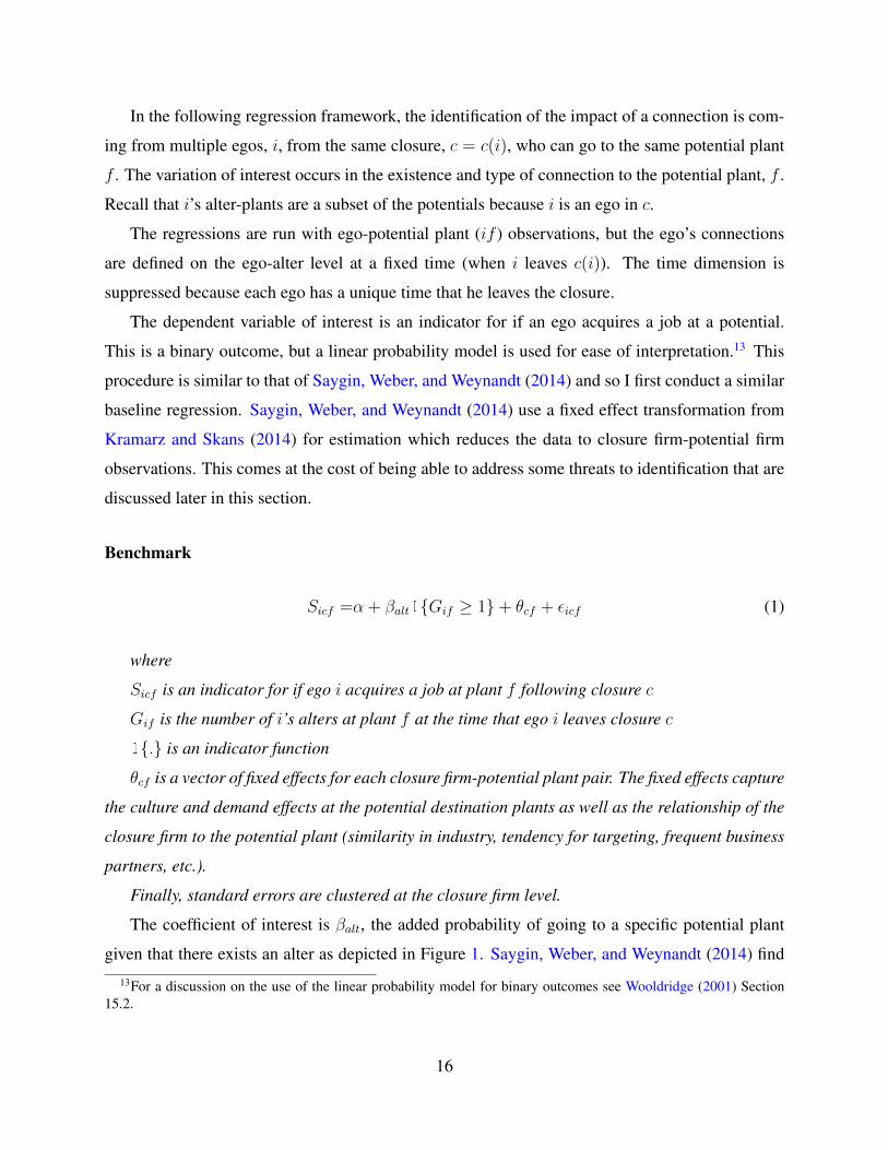
Sicf =α + βalt1{Gif ≥ 1}+ θcf + εicf (1)

where

Sicf is an indicator for if ego i acquires a job at plant f following closure c

Gif is the number of i’s alters at plant f at the time that ego i leaves closure c

1{.} is an indicator function

θcf is a vector of fixed effects for each closure firm-potential plant pair. The fixed effects capture

the culture and demand effects at the potential destination plants as well as the relationship of the

closure firm to the potential plant (similarity in industry, tendency for targeting, frequent business

partners, etc.).

Finally, standard errors are clustered at the closure firm level.

The coefficient of interest is βalt, the added probability of going to a specific potential plant

given that there exists an alter as depicted in Figure 1. Saygin, Weber, and Weynandt (2014) find

13For a discussion on the use of the linear probability model for binary outcomes see Wooldridge (2001) Section15.2.

16

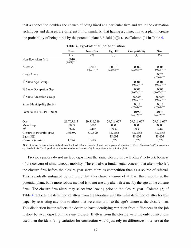
that a connection doubles the chance of being hired at a particular firm and while the estimation

techniques and datasets are different I find, similarly, that having a connection to a plant increase

the probability of being hired by the potential plant 3.3-fold ( .0010.0003

), see Column (1) in Table 4.

Table 4: Ego-Potential Job AcquisitionBase Non-Clos. Ego FE Compatibility Size(1) (2) (3) (4) (5)

Non-Ego Alters ≥ 1 .0010(.0001)∗∗∗

Alters ≥ 1 .0012 .0013 .0009 .0004(.0001)∗∗∗ (.0001)∗∗∗ (.0001)∗∗∗ (.00009)∗∗∗

(Log) Alters .0022(.0003)∗∗∗

% Same Age Group .0001 .0001(.00002)∗∗∗ (.00002)∗∗∗

% Same Occupation Grp. .0003 .0003(.00004)∗∗∗ (.00004)∗∗∗

% Same Education Group .00008 .00008(.00002)∗∗∗ (.00002)∗∗∗

Same Municipality (Indic) .0012 .0012(.0005)∗∗∗ (.0005)∗∗∗

Potential is Hist. Pl. (Indic) .0192 .0143(.0019)∗∗∗ (.0019)∗∗∗

Obs. 29,705,613 29,516,789 29,516,677 29,516,677 29,516,677Mean Dep. .0003 .0003 .0003 .0003 .0003R2 .2696 .2403 .2432 .2438 .244Closure × Potential (FE) 336,597 332,590 332,565 332,565 332,565Egos (FE) - - 38,603 38,603 38,603Closures (cluster) 1,724 1,697 1,672 1,672 1,672

Note: Standard errors clustered at the closure level. All columns contain closure firm × potential plant fixed effects. Columns (3)-(5) also containego fixed effects. The dependent variable is an indicator for an ego’s job acquisition at the potential plant.

Previous papers do not include egos from the same closure in each others’ network because

of the concern of simultaneous mobility. There is also a fundamental concern that alters who left

the closure firm before the closure year serve more as competition than as a source of referral.

This is partially mitigated by requiring that alters have a tenure of at least three months at the

potential plant, but a more robust method is to not use any alters first met by the ego at the closure

firm. The closure firm alters may select into leaving prior to the closure year. Column (2) of

Table 4 replaces the definition of alters from the literature with the main definition of alter for this

paper by restricting attention to alters that were met prior to the ego’s tenure at the closure firm.

This distinction better reflects the desire to have identifying variation from differences in the job

history between egos from the same closure. If alters from the closure were the only connections

used then the identifying variation for connection would just rely on differences in tenure at the

17

closure which is more susceptible to critiques surrounding endogenous mobility.14 Restricting to

this subset of alters results in a smaller sample because we lose some potential plants that only

employ closure alters and so no longer have identifying variation in the connection. Additionally,

the estimated coefficient is slightly larger, implying a 4-fold increase from a connection. The next

departure from the previous literature is to introduce ego fixed effects.

Ego Fixed Effects

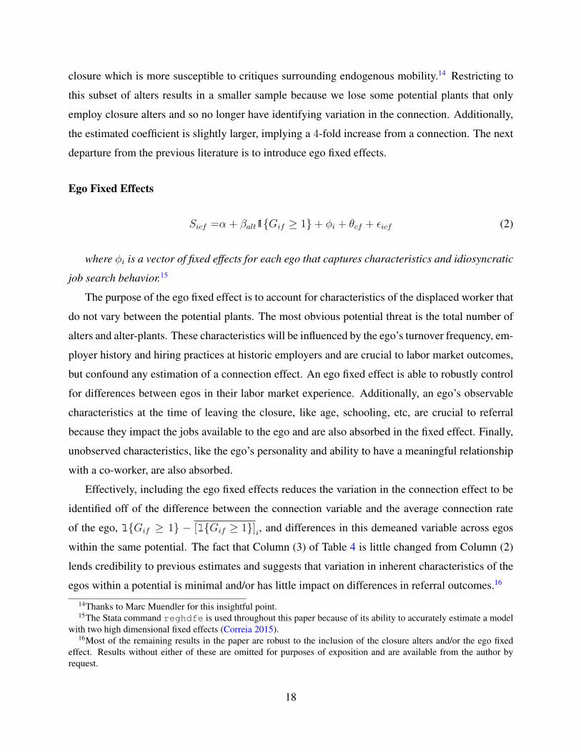
Sicf =α + βalt1{Gif ≥ 1}+ φi + θcf + εicf (2)

where φi is a vector of fixed effects for each ego that captures characteristics and idiosyncratic

job search behavior.15

The purpose of the ego fixed effect is to account for characteristics of the displaced worker that

do not vary between the potential plants. The most obvious potential threat is the total number of

alters and alter-plants. These characteristics will be influenced by the ego’s turnover frequency, em-

ployer history and hiring practices at historic employers and are crucial to labor market outcomes,

but confound any estimation of a connection effect. An ego fixed effect is able to robustly control

for differences between egos in their labor market experience. Additionally, an ego’s observable

characteristics at the time of leaving the closure, like age, schooling, etc, are crucial to referral

because they impact the jobs available to the ego and are also absorbed in the fixed effect. Finally,

unobserved characteristics, like the ego’s personality and ability to have a meaningful relationship

with a co-worker, are also absorbed.

Effectively, including the ego fixed effects reduces the variation in the connection effect to be

identified off of the difference between the connection variable and the average connection rate

of the ego, 1{Gif ≥ 1} − [1{Gif ≥ 1}]i, and differences in this demeaned variable across egos

within the same potential. The fact that Column (3) of Table 4 is little changed from Column (2)

lends credibility to previous estimates and suggests that variation in inherent characteristics of the

egos within a potential is minimal and/or has little impact on differences in referral outcomes.16

14Thanks to Marc Muendler for this insightful point.15The Stata command reghdfe is used throughout this paper because of its ability to accurately estimate a model

with two high dimensional fixed effects (Correia 2015).16Most of the remaining results in the paper are robust to the inclusion of the closure alters and/or the ego fixed

effect. Results without either of these are omitted for purposes of exposition and are available from the author byrequest.

18

The two sets of fixed effects account for similarities between the closure and destination plant

and the ego’s idiosyncratic characteristics, but not the similarity between ego i and the potential

hiring plant f . Without relying on a connection, it is plausible that f targets individuals like i,

or i is more likely to look to plant f , if f has more employees like i. Additionally, aspects of f

such as how it relates to i’s labor market experience are important. It is necessary to control for

observable compatibility between the ego and potential. Targeting on unobservable characteristics

is addressed in Section 6.

Compatibility

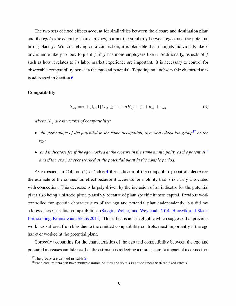
Sicf =α + βalt1{Gif ≥ 1}+ δHif + φi + θcf + εicf (3)

where Hif are measures of compatibility:

• the percentage of the potential in the same occupation, age, and education group17 as the

ego

• and indicators for if the ego worked at the closure in the same municipality as the potential18

and if the ego has ever worked at the potential plant in the sample period.

As expected, in Column (4) of Table 4 the inclusion of the compatibility controls decreases

the estimate of the connection effect because it accounts for mobility that is not truly associated

with connection. This decrease is largely driven by the inclusion of an indicator for the potential

plant also being a historic plant, plausibly because of plant specific human capital. Previous work

controlled for specific characteristics of the ego and potential plant independently, but did not

address these baseline compatibilities (Saygin, Weber, and Weynandt 2014, Hensvik and Skans

forthcoming, Kramarz and Skans 2014). This effect is non-negligible which suggests that previous

work has suffered from bias due to the omitted compatibility controls, most importantly if the ego

has ever worked at the potential plant.

Correctly accounting for the characteristics of the ego and compatibility between the ego and

potential increases confidence that the estimate is reflecting a more accurate impact of a connection

17The groups are defined in Table 2.18Each closure firm can have multiple municipalities and so this is not collinear with the fixed effects.

19

on the probability of being hired. To understand the referral mechanism it is important to explore

variation between connections.

One source of variation in connection that is often overlooked is the number of connections to

a potential plant. This is important because multiple alters at a plant could have complementary

effects on referral and/or the number of alters at a firm is correlated with the number of those alters

that the ego has a strong working relationship with. The latter point is especially important because

when referral is inferred from mobility there is no assurance of a “true” relationship between the

ego and alter. The chance of a relationship given one alter is substantially different from the chance

of a relationship given five. To understand this variability I now introduce a control for the (log)

number of alters that an ego has at a specific potential. Given that log(0) is undefined I set the log

number of alters to 0 if there are no alters. This can be interpreted as an interaction between the

indicator and the log term. The addition of the log term changes the interpretation of βalt from the

impact of going from no alters to any alters to now represent the impact of going from no alters to

one alter, while the log term captures the impact of increases in the number of alters.

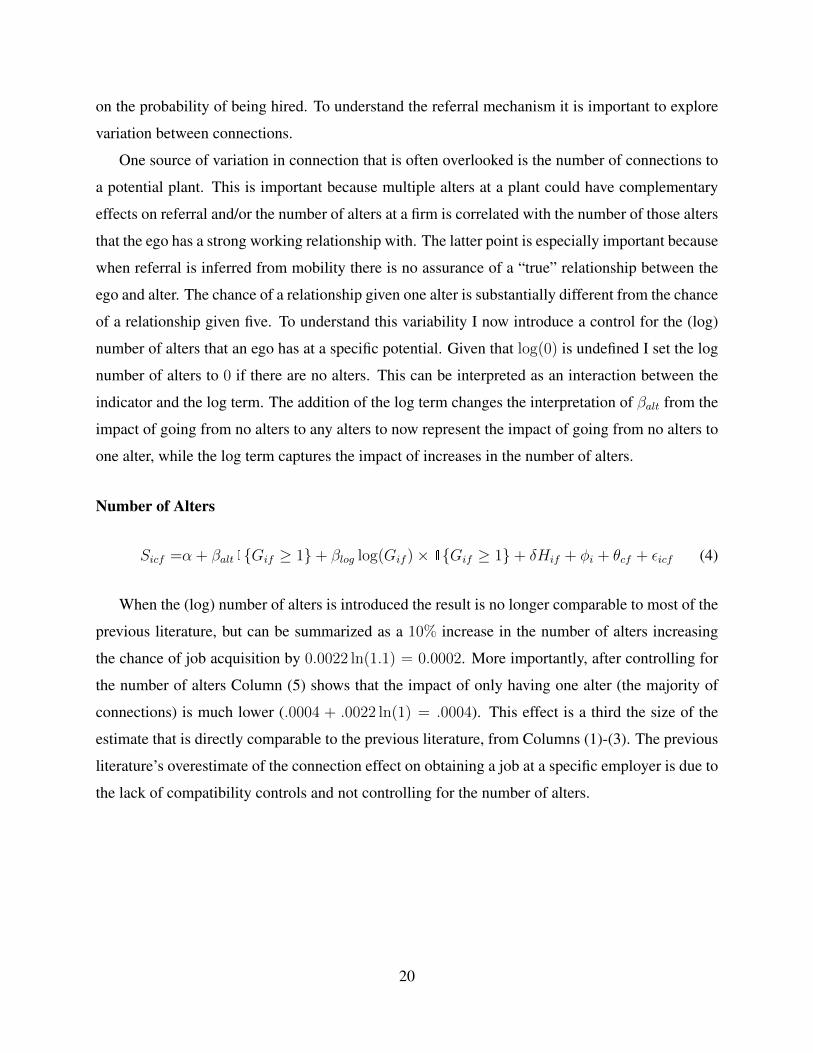
Number of Alters

Sicf =α + βalt1{Gif ≥ 1}+ βlog log(Gif )× 1{Gif ≥ 1}+ δHif + φi + θcf + εicf (4)

When the (log) number of alters is introduced the result is no longer comparable to most of the

previous literature, but can be summarized as a 10% increase in the number of alters increasing

the chance of job acquisition by 0.0022 ln(1.1) = 0.0002. More importantly, after controlling for

the number of alters Column (5) shows that the impact of only having one alter (the majority of

connections) is much lower (.0004 + .0022 ln(1) = .0004). This effect is a third the size of the

estimate that is directly comparable to the previous literature, from Columns (1)-(3). The previous

literature’s overestimate of the connection effect on obtaining a job at a specific employer is due to

the lack of compatibility controls and not controlling for the number of alters.

20

5 Hiring-Cohort: Relationships with some co-workers are more

likely than others

I now turn to the central point of the paper and focus on the added impact of the hiring-cohort

co-workers. As developed in Chen-Zion and Rauch (2016), theory predicts that cohort-alters are

more likely to have had a working relationship with the ego and so are more likely to provide a

meaningful connection to a potential workplace. I begin with a quick overview of the theory and

then turn to specifications that include the cohort effect.

5.1 Theory of Hiring-Cohort Attachment

Chen-Zion and Rauch (2016) model matches between workers within a firm, much like Jovanovic

(1979) models workers and firms matching in the labor market. Well-matched workers become

members of each others’ networks (stay together), and poorly matched workers avoid each other in

the future (separate). The model allows matches with any number of other agents, up to the limit of

all the agents in the firm, but with a convex cost. The ego has an optimal number or relationships

and fills them with well-matched workers before attempting to find new alters to work with.

Proposition 1 (Chen-Zion and Rauch 2016). Egos become monotonically less open over time to

meeting alters of unknown match quality.

This occurs because the ego’s network degree increases monotonically with time as he acquires

more high quality connections whereas his optimally chosen capacity for work relationships re-

mains unchanged.

This leads to cohort attachment because when the ego’s cohort enters the incumbent workers

all have established relationships, and are less open to forming new relationships, while the fellow

entrants all have no connections and so are especially likely to match with each other. This gives

rise to an ego developing a working relationship with others from his/her cohort that continues

over time. Those that the ego matched with initially, and found to be of high quality, remain in the

network indefinitely if the relationship quality remains known.

The takeaway is that persistence in interaction leads to the cohort-alters being a large portion

of the ego’s network of work relationships. The importance of the work connections is that the

persistence relies on having a good relationship. This good relationship might change slightly over

21

time (captured by knowledge loss in Chen-Zion and Rauch (2016)), but it also translates from one

firm to the next. If an alter and ego were to stop working together the knowledge of their good

relationship would persist with each.

When the ego leaves the firm the job search process begins. The model for job referral that

motivates the following analysis is one in which the hiring manager only acts on positive referrals

from their employees/colleagues and where a worker makes a referral to the hiring manager so that

they can benefit from renewing their positive work relationship.

The fact that relationships persist and cohort-alters are more likely to have had relationships

means that the ego is likely to end up at a firm where said cohort-alters are currently employed

because the cohort-alters recommended them to the hiring manager.

The predictions outlined above do not have magnitudes so it is important to empirically test if

cohort attachment is meaningfully present in the job acquisition process. To test this I return to the

regression specification of Table 4 Column (5) to assess the marginal contribution of a cohort-alter.

5.2 Results

The summary statistics in Table 3 show that of the 3.1% of observations with at least one alter

22.9% (84.9%) have at least one (non-)cohort-alter. These classifications are not mutually exclu-

sive because potential plants with two alters could have both a cohort and a non-cohort alter. As

highlighted in Section 3, the chance of obtaining a job at a specific potential increases (.003 to

.008) for observations with a cohort-alter, but this occurs with a simultaneous increase in the num-

ber of alters (conditional on positive 5.2 to 17.4) and compatibility between the ego and potential

(e.g. the fraction in the same education group as the ego: 56.9% to 63.2%). As before, to separate

these simultaneous effects I return back to the regression specification. In Table 5, I decompose

the alters by their cohort status and study the impact of the potential plant having cohort-alters and

non-cohort-alters.

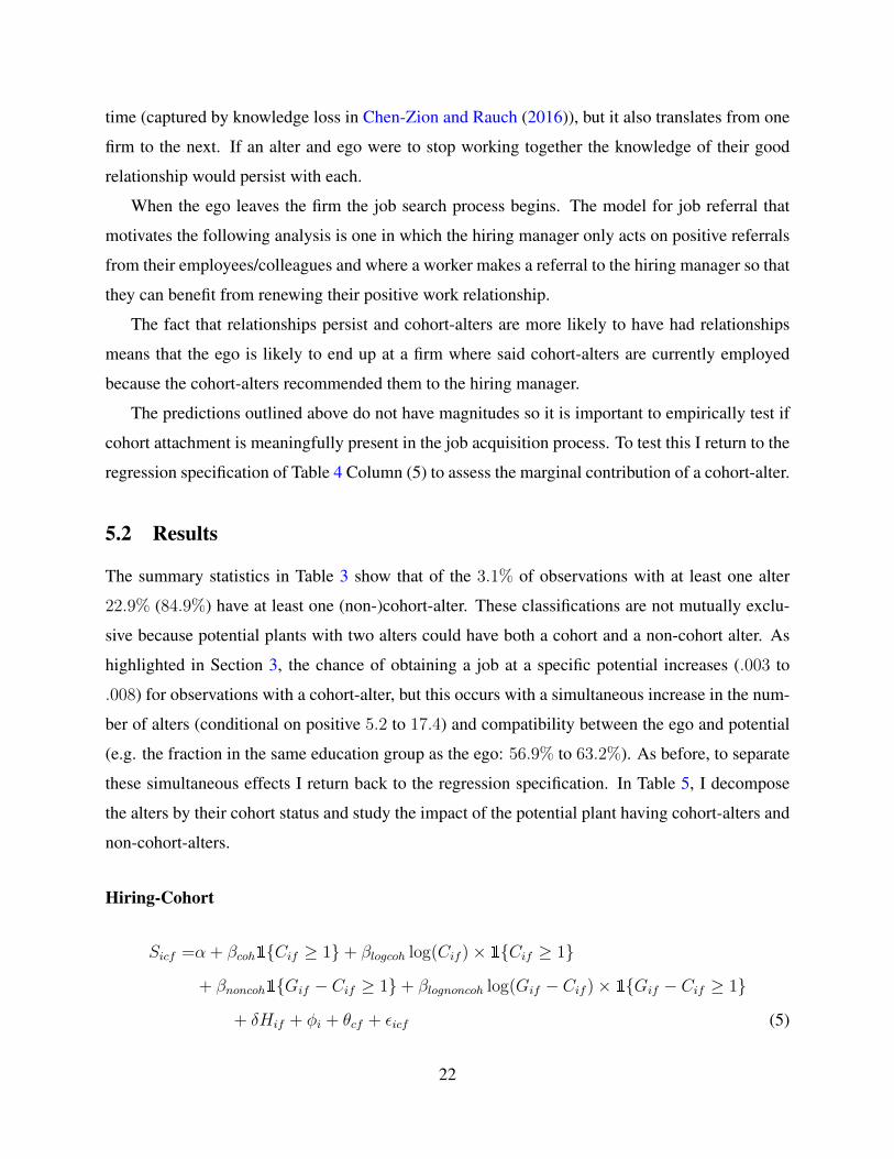
Hiring-Cohort

Sicf =α + βcoh1{Cif ≥ 1}+ βlogcoh log(Cif )× 1{Cif ≥ 1}

+ βnoncoh1{Gif − Cif ≥ 1}+ βlognoncoh log(Gif − Cif )× 1{Gif − Cif ≥ 1}

+ δHif + φi + θcf + εicf (5)

22

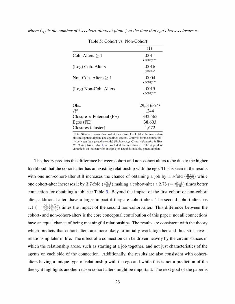
where Cif is the number of i’s cohort-alters at plant f at the time that ego i leaves closure c.

Table 5: Cohort vs. Non-Cohort

(1)

Coh. Alters ≥ 1 .0011(.0002)∗∗∗

(Log) Coh. Alters .0016(.0008)∗

Non-Coh. Alters ≥ 1 .0004(.0001)∗∗∗

(Log) Non-Coh. Alters .0015(.0003)∗∗∗

Obs. 29,516,677R2 .244Closure × Potential (FE) 332,565Egos (FE) 38,603Closures (cluster) 1,672Note: Standard errors clustered at the closure level. All columns contain

closure×potential plant and ego fixed effects. Controls for the compatibil-ity between the ego and potential (% Same Age Group – Potential is Hist.Pl. (Indic) from Table 4) are included, but not shown. The dependentvariable is an indicator for an ego’s job acquisition at the potential plant.

The theory predicts this difference between cohort and non-cohort alters to be due to the higher

likelihood that the cohort-alter has an existing relationship with the ego. This is seen in the results

with one non-cohort-alter still increases the chance of obtaining a job by 1.3-fold ( .0004.0003

) while

one cohort-alter increases it by 3.7-fold ( .0011.0003

) making a cohort-alter a 2.75 (= .0011.0004

) times better

connection for obtaining a job, see Table 5. Beyond the impact of the first cohort or non-cohort

alter, additional alters have a larger impact if they are cohort-alter. The second cohort-alter has

1.1 (= .0016 ln(2).0015 ln(2)

) times the impact of the second non-cohort-alter. This difference between the

cohort- and non-cohort-alters is the core conceptual contribution of this paper: not all connections

have an equal chance of being meaningful relationships. The results are consistent with the theory

which predicts that cohort-alters are more likely to initially work together and thus still have a

relationship later in life. The effect of a connection can be driven heavily by the circumstances in

which the relationship arose, such as starting at a job together, and not just characteristics of the

agents on each side of the connection. Additionally, the results are also consistent with cohort-

alters having a unique type of relationship with the ego and while this is not a prediction of the

theory it highlights another reason cohort-alters might be important. The next goal of the paper is

23

to verify that there are not alternative mechanisms driving the connection and/or cohort effects.19

6 Robustness to Alternative Explanations

The following verify that the previous results are coming from the impact of a connection, and not

unobservable characteristics correlated with hiring, by using (i) placebo histories (Section 6.1), (ii)

placebo destinations (Section 6.2) (iii) alter characteristics (Section 6.3), and (iv) instruments for

connection (Section 6.4).

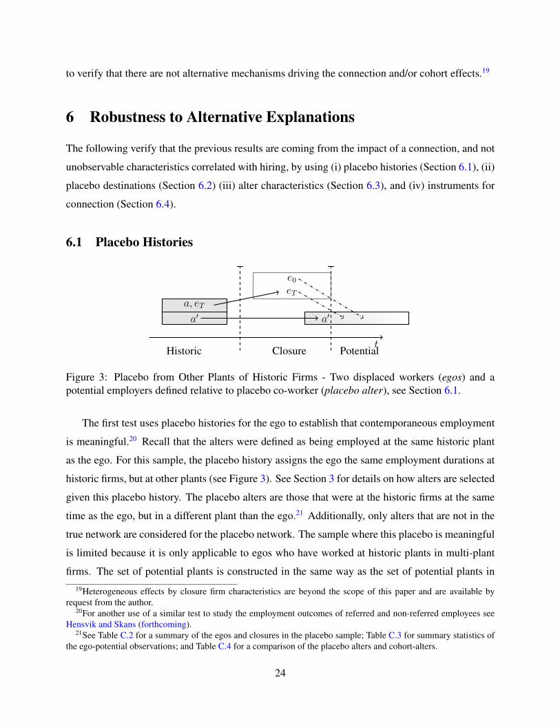
6.1 Placebo Histories

Historic Closure Potentialt

a, eT

e0eT

a′ a′

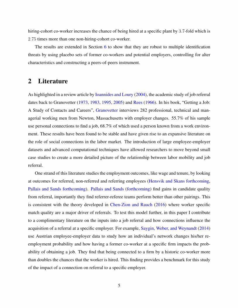
Figure 3: Placebo from Other Plants of Historic Firms - Two displaced workers (egos) and apotential employers defined relative to placebo co-worker (placebo alter), see Section 6.1.

The first test uses placebo histories for the ego to establish that contemporaneous employment

is meaningful.20 Recall that the alters were defined as being employed at the same historic plant

as the ego. For this sample, the placebo history assigns the ego the same employment durations at

historic firms, but at other plants (see Figure 3). See Section 3 for details on how alters are selected

given this placebo history. The placebo alters are those that were at the historic firms at the same

time as the ego, but in a different plant than the ego.21 Additionally, only alters that are not in the

true network are considered for the placebo network. The sample where this placebo is meaningful

is limited because it is only applicable to egos who have worked at historic plants in multi-plant

firms. The set of potential plants is constructed in the same way as the set of potential plants in19Heterogeneous effects by closure firm characteristics are beyond the scope of this paper and are available by

request from the author.20For another use of a similar test to study the employment outcomes of referred and non-referred employees see

Hensvik and Skans (forthcoming).21See Table C.2 for a summary of the egos and closures in the placebo sample; Table C.3 for summary statistics of

the ego-potential observations; and Table C.4 for a comparison of the placebo alters and cohort-alters.

24

the baseline specification, but using placebo alters in place of true alters. The set of potentials is

different because all the egos have new sets of plants connected by placebo alters resulting in fewer

ego-potential observations.

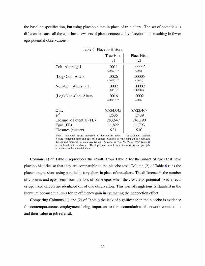
Table 6: Placebo History

True Hist. Plac. Hist.(1) (2)

Coh. Alters ≥ 1 .0011 -.00002(.0002)∗∗∗ (.0001)

(Log) Coh. Alters .0026 .00005(.0009)∗∗∗ (.0004)

Non-Coh. Alters ≥ 1 .0002 .00002(.0001)∗ (.00006)

(Log) Non-Coh. Alters .0016 .0002(.0004)∗∗∗ (.0002)

Obs. 9,734,045 8,723,467R2 .2535 .2439Closure × Potential (FE) 283,647 241,190Egos (FE) 11,822 11,793Closures (cluster) 921 910Note: Standard errors clustered at the closure level. All columns contain

closure×potential plant and ego fixed effects. Controls for the compatibility betweenthe ego and potential (% Same Age Group – Potential is Hist. Pl. (Indic) from Table 4)are included, but not shown. The dependent variable is an indicator for an ego’s jobacquisition at the potential plant.

Column (1) of Table 6 reproduces the results from Table 5 for the subset of egos that have

placebo histories so that they are comparable to the placebo test. Column (2) of Table 6 runs the

placebo regressions using parallel history alters in place of true alters. The difference in the number

of closures and egos stem from the loss of some egos when the closure × potential fixed effects

or ego fixed effects are identified off of one observation. This loss of singletons is standard in the

literature because it allows for an efficiency gain in estimating the connection effect.

Comparing Columns (1) and (2) of Table 6 the lack of significance in the placebo is evidence

for contemporaneous employment being important to the accumulation of network connections

and their value in job referral.

25

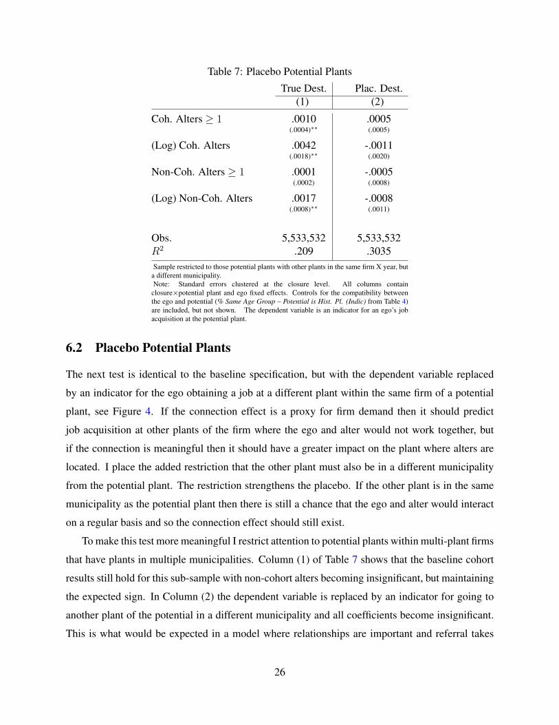
Table 7: Placebo Potential Plants

True Dest. Plac. Dest.(1) (2)

Coh. Alters ≥ 1 .0010 .0005(.0004)∗∗ (.0005)

(Log) Coh. Alters .0042 -.0011(.0018)∗∗ (.0020)

Non-Coh. Alters ≥ 1 .0001 -.0005(.0002) (.0008)

(Log) Non-Coh. Alters .0017 -.0008(.0008)∗∗ (.0011)

Obs. 5,533,532 5,533,532R2 .209 .3035Sample restricted to those potential plants with other plants in the same firm X year, but

a different municipality.Note: Standard errors clustered at the closure level. All columns contain

closure×potential plant and ego fixed effects. Controls for the compatibility betweenthe ego and potential (% Same Age Group – Potential is Hist. Pl. (Indic) from Table 4)are included, but not shown. The dependent variable is an indicator for an ego’s jobacquisition at the potential plant.

6.2 Placebo Potential Plants

The next test is identical to the baseline specification, but with the dependent variable replaced

by an indicator for the ego obtaining a job at a different plant within the same firm of a potential

plant, see Figure 4. If the connection effect is a proxy for firm demand then it should predict

job acquisition at other plants of the firm where the ego and alter would not work together, but

if the connection is meaningful then it should have a greater impact on the plant where alters are

located. I place the added restriction that the other plant must also be in a different municipality

from the potential plant. The restriction strengthens the placebo. If the other plant is in the same

municipality as the potential plant then there is still a chance that the ego and alter would interact

on a regular basis and so the connection effect should still exist.

To make this test more meaningful I restrict attention to potential plants within multi-plant firms

that have plants in multiple municipalities. Column (1) of Table 7 shows that the baseline cohort

results still hold for this sub-sample with non-cohort alters becoming insignificant, but maintaining

the expected sign. In Column (2) the dependent variable is replaced by an indicator for going to

another plant of the potential in a different municipality and all coefficients become insignificant.

This is what would be expected in a model where relationships are important and referral takes

26

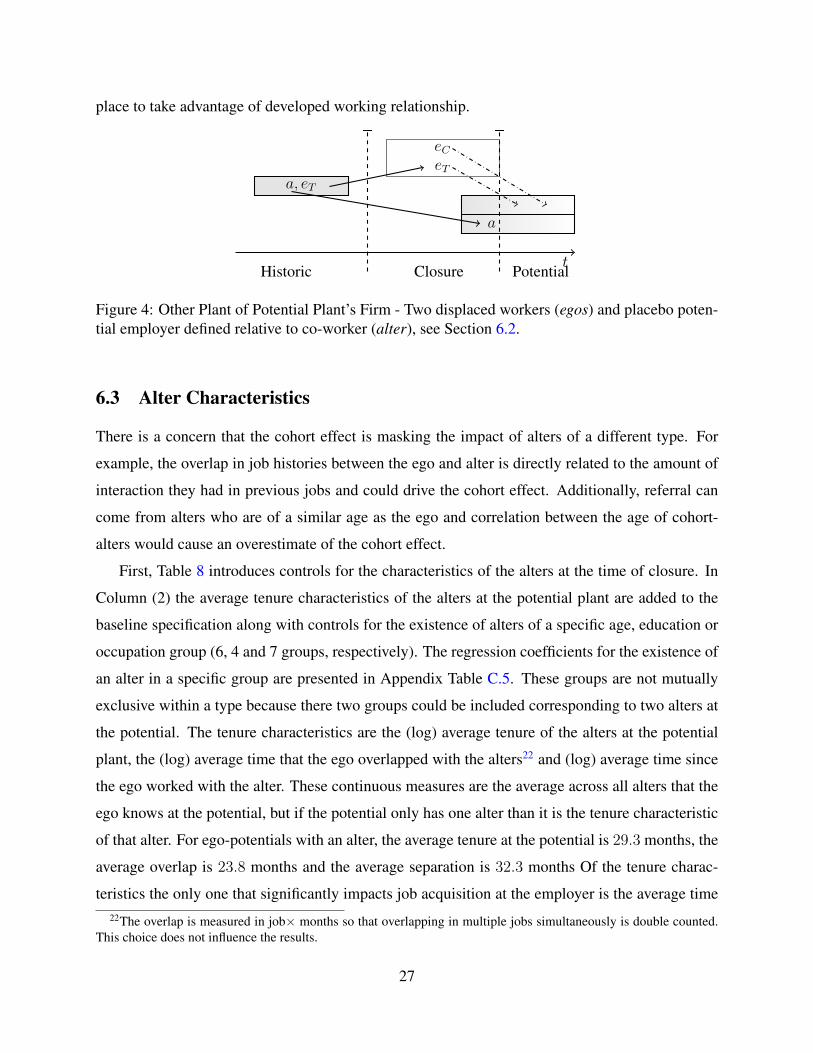
place to take advantage of developed working relationship.

Historic Closure Potentialt

a, eT

eCeT

a

Figure 4: Other Plant of Potential Plant’s Firm - Two displaced workers (egos) and placebo poten-tial employer defined relative to co-worker (alter), see Section 6.2.

6.3 Alter Characteristics

There is a concern that the cohort effect is masking the impact of alters of a different type. For

example, the overlap in job histories between the ego and alter is directly related to the amount of

interaction they had in previous jobs and could drive the cohort effect. Additionally, referral can

come from alters who are of a similar age as the ego and correlation between the age of cohort-

alters would cause an overestimate of the cohort effect.

First, Table 8 introduces controls for the characteristics of the alters at the time of closure. In

Column (2) the average tenure characteristics of the alters at the potential plant are added to the

baseline specification along with controls for the existence of alters of a specific age, education or

occupation group (6, 4 and 7 groups, respectively). The regression coefficients for the existence of

an alter in a specific group are presented in Appendix Table C.5. These groups are not mutually

exclusive within a type because there two groups could be included corresponding to two alters at

the potential. The tenure characteristics are the (log) average tenure of the alters at the potential

plant, the (log) average time that the ego overlapped with the alters22 and (log) average time since

the ego worked with the alter. These continuous measures are the average across all alters that the

ego knows at the potential, but if the potential only has one alter than it is the tenure characteristic

of that alter. For ego-potentials with an alter, the average tenure at the potential is 29.3 months, the

average overlap is 23.8 months and the average separation is 32.3 months Of the tenure charac-

teristics the only one that significantly impacts job acquisition at the employer is the average time22The overlap is measured in job× months so that overlapping in multiple jobs simultaneously is double counted.

This choice does not influence the results.

27

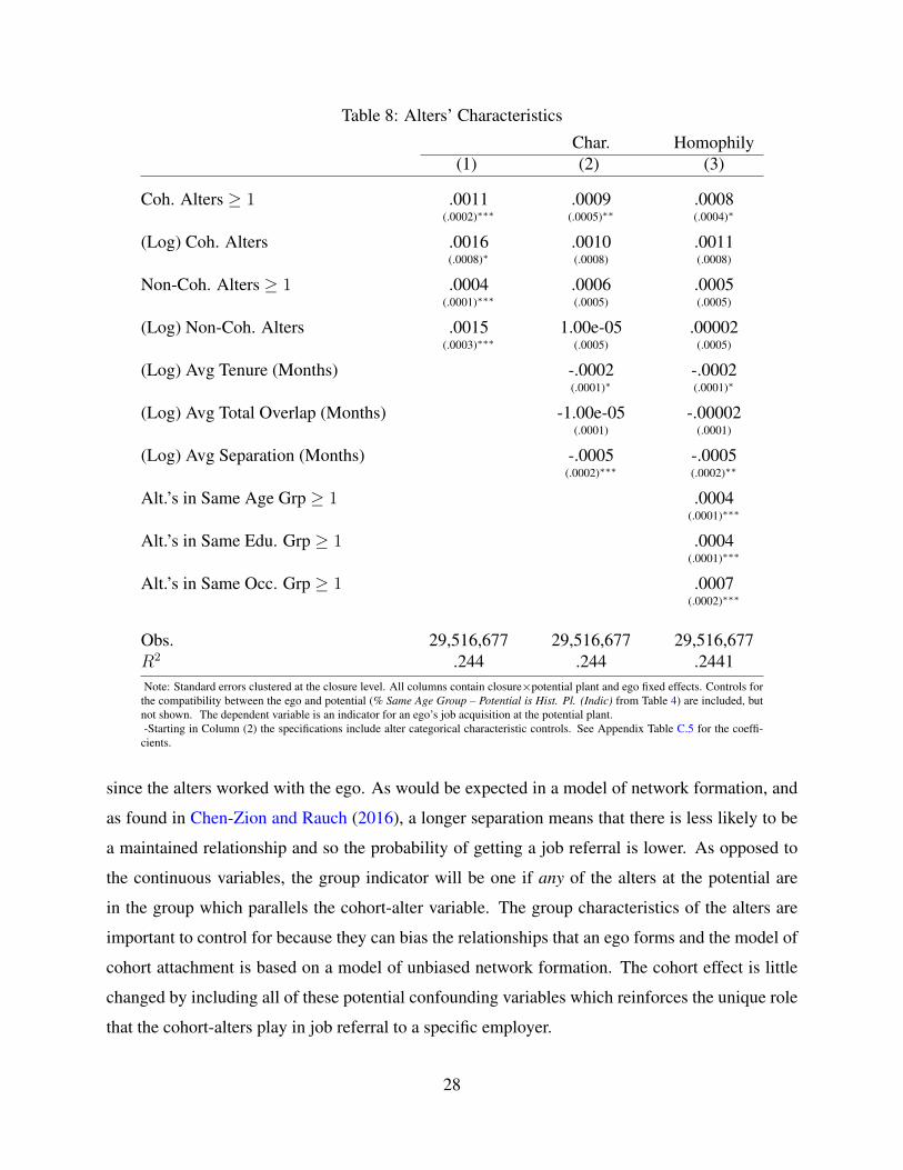
Table 8: Alters’ Characteristics

Char. Homophily(1) (2) (3)

Coh. Alters ≥ 1 .0011 .0009 .0008(.0002)∗∗∗ (.0005)∗∗ (.0004)∗

(Log) Coh. Alters .0016 .0010 .0011(.0008)∗ (.0008) (.0008)

Non-Coh. Alters ≥ 1 .0004 .0006 .0005(.0001)∗∗∗ (.0005) (.0005)

(Log) Non-Coh. Alters .0015 1.00e-05 .00002(.0003)∗∗∗ (.0005) (.0005)

(Log) Avg Tenure (Months) -.0002 -.0002(.0001)∗ (.0001)∗

(Log) Avg Total Overlap (Months) -1.00e-05 -.00002(.0001) (.0001)

(Log) Avg Separation (Months) -.0005 -.0005(.0002)∗∗∗ (.0002)∗∗

Alt.’s in Same Age Grp ≥ 1 .0004(.0001)∗∗∗

Alt.’s in Same Edu. Grp ≥ 1 .0004(.0001)∗∗∗

Alt.’s in Same Occ. Grp ≥ 1 .0007(.0002)∗∗∗

Obs. 29,516,677 29,516,677 29,516,677R2 .244 .244 .2441Note: Standard errors clustered at the closure level. All columns contain closure×potential plant and ego fixed effects. Controls for

the compatibility between the ego and potential (% Same Age Group – Potential is Hist. Pl. (Indic) from Table 4) are included, butnot shown. The dependent variable is an indicator for an ego’s job acquisition at the potential plant.-Starting in Column (2) the specifications include alter categorical characteristic controls. See Appendix Table C.5 for the coeffi-

cients.

since the alters worked with the ego. As would be expected in a model of network formation, and

as found in Chen-Zion and Rauch (2016), a longer separation means that there is less likely to be

a maintained relationship and so the probability of getting a job referral is lower. As opposed to

the continuous variables, the group indicator will be one if any of the alters at the potential are

in the group which parallels the cohort-alter variable. The group characteristics of the alters are

important to control for because they can bias the relationships that an ego forms and the model of

cohort attachment is based on a model of unbiased network formation. The cohort effect is little

changed by including all of these potential confounding variables which reinforces the unique role

that the cohort-alters play in job referral to a specific employer.

28

Controlling for the characteristics of the alters is important and the ego fixed effects effectively

control for the ego characteristics. This decomposition of job referral based on the job seeker char-

acteristics and referrer characteristics is understood. For example, there are a number of papers

studying job referral within minority groups, with the assumption that there is likely to be more

interaction both on and off work (Dustmann, Glitz, Schonberg, and Bruecker forthcoming, Kerr

and Mandorff 2015). This paper is taking a complementary perspective and seeking to understand

how differences in the the likelihood of a meaningful relationship impact referral. This concept

is distinct from much of the other job referral literature which might focus on a broad category

of relationships, like familial, with minimal comparison to vastly different types of relationships,

like co-workers. While interesting, the benefit of understanding these difference has limited impli-

cations because the conversion of workplace relationships to familial relationships is not a policy

relevant action. In comparison, the result of studying differences among co-worker relationships

could yield implications for hiring policies.

If the focus is on the relationship, then beyond controlling for the characteristics of the alters

it is also important to control for how similar the ego and alters are along observable dimensions.

This is because homophily, the tendency of agents to be more likely to interact with others with

similar observable traits, is a known phenomenon (McPherson, Smith-Lovin, and Cook 2001). In

Column (3) I add additional controls for homophily between the ego and alters at the potential: an

indicator for the existence of an alter in the ego’s age, occupation and education groups. For ego-

potentials with alters the fraction with at least one alter in the ego’s age, occupation and education

group is 35.9%, 45.0% and 61.5%, respectively. The resulting homophily effects are significant,

but do not substantially change the cohort or (log) number of alters effects. The differences in

the homophily effects reflect meaningful differences in job referral. Most importantly, if an alter

is in the same occupation group as the ego he/she would be most able to assess the ego’s skills

in the field. Even with this proxy for common skills the cohort effect remains significant which

highlights that the impact of a relationship transcends observable categories.

6.4 Instrument for Alters’ Location

When considering a peer or network effects model, as this paper does, there are multiple sources

of endogeneity that the literature has recognized as potentially concerning. All of these sources

focus on how the existence of a connection Wif ([cohort-alters, non-cohort-alters] × [≥ 1, log])

29

Alters’ Alters

Alters

EgoFirm Alt Alt AltBlack 1 1White 1 3Grey 1 0Diamond 0 1

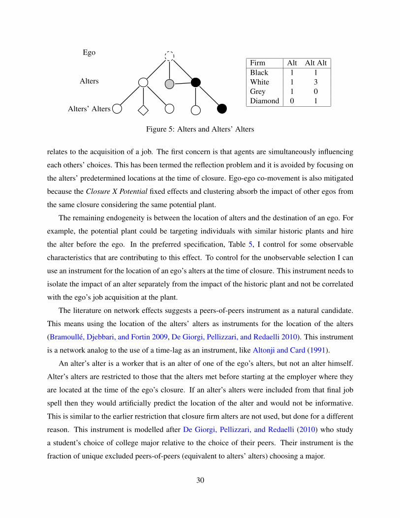
Figure 5: Alters and Alters’ Alters

relates to the acquisition of a job. The first concern is that agents are simultaneously influencing

each others’ choices. This has been termed the reflection problem and it is avoided by focusing on

the alters’ predetermined locations at the time of closure. Ego-ego co-movement is also mitigated

because the Closure X Potential fixed effects and clustering absorb the impact of other egos from

the same closure considering the same potential plant.

The remaining endogeneity is between the location of alters and the destination of an ego. For

example, the potential plant could be targeting individuals with similar historic plants and hire

the alter before the ego. In the preferred specification, Table 5, I control for some observable

characteristics that are contributing to this effect. To control for the unobservable selection I can

use an instrument for the location of an ego’s alters at the time of closure. This instrument needs to

isolate the impact of an alter separately from the impact of the historic plant and not be correlated

with the ego’s job acquisition at the plant.

The literature on network effects suggests a peers-of-peers instrument as a natural candidate.

This means using the location of the alters’ alters as instruments for the location of the alters

(Bramoulle, Djebbari, and Fortin 2009, De Giorgi, Pellizzari, and Redaelli 2010). This instrument

is a network analog to the use of a time-lag as an instrument, like Altonji and Card (1991).

An alter’s alter is a worker that is an alter of one of the ego’s alters, but not an alter himself.

Alter’s alters are restricted to those that the alters met before starting at the employer where they

are located at the time of the ego’s closure. If an alter’s alters were included from that final job

spell then they would artificially predict the location of the alter and would not be informative.

This is similar to the earlier restriction that closure firm alters are not used, but done for a different

reason. This instrument is modelled after De Giorgi, Pellizzari, and Redaelli (2010) who study

a student’s choice of college major relative to the choice of their peers. Their instrument is the

fraction of unique excluded peers-of-peers (equivalent to alters’ alters) choosing a major.

30

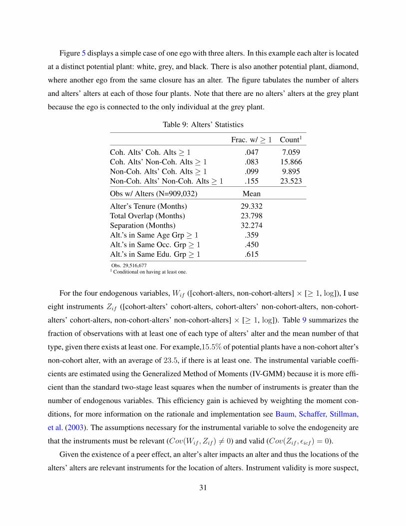
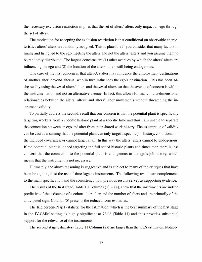
Figure 5 displays a simple case of one ego with three alters. In this example each alter is located

at a distinct potential plant: white, grey, and black. There is also another potential plant, diamond,

where another ego from the same closure has an alter. The figure tabulates the number of alters

and alters’ alters at each of those four plants. Note that there are no alters’ alters at the grey plant

because the ego is connected to the only individual at the grey plant.

Table 9: Alters’ Statistics

Frac. w/ ≥ 1 Count1

Coh. Alts’ Coh. Alts ≥ 1 .047 7.059Coh. Alts’ Non-Coh. Alts ≥ 1 .083 15.866Non-Coh. Alts’ Coh. Alts ≥ 1 .099 9.895Non-Coh. Alts’ Non-Coh. Alts ≥ 1 .155 23.523

Obs w/ Alters (N=909,032) Mean

Alter’s Tenure (Months) 29.332Total Overlap (Months) 23.798Separation (Months) 32.274Alt.’s in Same Age Grp ≥ 1 .359Alt.’s in Same Occ. Grp ≥ 1 .450Alt.’s in Same Edu. Grp ≥ 1 .615Obs. 29,516,677

1 Conditional on having at least one.

For the four endogenous variables, Wif ([cohort-alters, non-cohort-alters] × [≥ 1, log]), I use

eight instruments Zif ([cohort-alters’ cohort-alters, cohort-alters’ non-cohort-alters, non-cohort-

alters’ cohort-alters, non-cohort-alters’ non-cohort-alters] × [≥ 1, log]). Table 9 summarizes the

fraction of observations with at least one of each type of alters’ alter and the mean number of that

type, given there exists at least one. For example,15.5% of potential plants have a non-cohort alter’s

non-cohort alter, with an average of 23.5, if there is at least one. The instrumental variable coeffi-

cients are estimated using the Generalized Method of Moments (IV-GMM) because it is more effi-

cient than the standard two-stage least squares when the number of instruments is greater than the

number of endogenous variables. This efficiency gain is achieved by weighting the moment con-

ditions, for more information on the rationale and implementation see Baum, Schaffer, Stillman,

et al. (2003). The assumptions necessary for the instrumental variable to solve the endogeneity are

that the instruments must be relevant (Cov(Wif , Zif ) 6= 0) and valid (Cov(Zif , εicf ) = 0).

Given the existence of a peer effect, an alter’s alter impacts an alter and thus the locations of the

alters’ alters are relevant instruments for the location of alters. Instrument validity is more suspect,

31

the necessary exclusion restriction implies that the set of alters’ alters only impact an ego through

the set of alters.

The motivation for accepting the exclusion restriction is that conditional on observable charac-

teristics alters’ alters are randomly assigned. This is plausible if you consider that many factors in

hiring and firing led to the ego meeting the alters and not the alters’ alters and you assume them to

be randomly distributed. The largest concerns are (1) other avenues by which the alters’ alters are

influencing the ego and (2) the location of the alters’ alters still being endogenous.

One case of the first concern is that alter-A’s alter may influence the employment destinations

of another alter, beyond alter-A, who in turn influences the ego’s destination. This has been ad-

dressed by using the set of alters’ alters and the set of alters, so that the avenue of concern is within

the instrumentation and not an alternative avenue. In fact, this allows for many multi-dimensional

relationships between the alters’ alters’ and alters’ labor movements without threatening the in-

strument validity.

To partially address the second, recall that one concern is that the potential plant is specifically

targeting workers from a specific historic plant at a specific time and thus I am unable to separate

the connection between an ego and alter from their shared work history. The assumption of validity

can be cast as assuming that the potential plant can only target a specific job history, conditional on

the included covariates, or cannot target at all. In this way the alters’ alters cannot be endogenous.

If the potential plant is indeed targeting the full set of historic plants and times then there is less

concern that the connection to the potential plant is endogenous to the ego’s job history, which

means that the instrument is not necessary.

Ultimately, the above reasoning is suggestive and is subject to many of the critiques that have

been brought against the use of time-lags as instruments. The following results are complements

to the main specification and the consistency with previous results serves as supporting evidence.

The results of the first stage, Table 10 Columns (1)− (4), show that the instruments are indeed

predictive of the existence of a cohort-alter, alter and the number of alters and are primarily of the

anticipated sign. Column (5) presents the reduced form estimates.

The Kleibergen-Paap F-statistic for the estimation, which is the best summary of the first stage

in the IV-GMM setting, is highly significant at 75.08 (Table 11) and thus provides substantial

support for the relevance of the instruments.

The second stage estimates (Table 11 Column (2)) are larger than the OLS estimates. Notably,

32

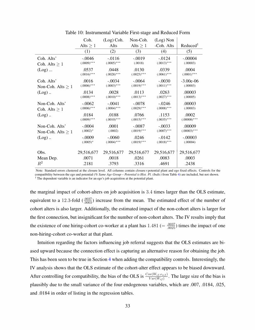
Table 10: Instrumental Variable First-stage and Reduced FormCoh. (Log) Coh. Non-Coh. (Log) Non

Alts ≥ 1 Alts Alts ≥ 1 -Coh. Alts Reduced1

(1) (2) (3) (4) (5)

Coh. Alts’ -.0046 -.0116 -.0019 -.0124 -.00004Coh. Alts ≥ 1 (.0009)∗∗∗ (.0005)∗∗∗ (.0018) (.0013)∗∗∗ (.00003)

(Log) ... .0537 .0448 .0130 .0339 .0004(.0016)∗∗∗ (.0028)∗∗∗ (.0025)∗∗∗ (.0061)∗∗∗ (.0001)∗∗∗

Coh. Alts’ .0016 -.0034 -.0064 -.0030 -3.00e-06Non-Coh. Alts ≥ 1 (.0006)∗∗∗ (.0003)∗∗∗ (.0019)∗∗∗ (.0011)∗∗∗ (.00003)

(Log) .. .0134 .0028 .0113 .0263 .00003(.0008)∗∗∗ (.0010)∗∗∗ (.0013)∗∗∗ (.0027)∗∗∗ (.00005)

Non-Coh. Alts’ -.0062 -.0041 -.0078 -.0246 .00003Coh. Alts ≥ 1 (.0006)∗∗∗ (.0004)∗∗∗ (.0029)∗∗∗ (.0008)∗∗∗ (.00003)

(Log) .. .0184 .0188 .0766 .1153 .0002(.0009)∗∗∗ (.0010)∗∗∗ (.0015)∗∗∗ (.0035)∗∗∗ (.00008)∗∗∗

Non-Coh. Alts’ -.0004 .0001 -.0087 -.0033 .00009Non-Coh. Alts ≥ 1 (.0002)∗ (.0002) (.0019)∗∗∗ (.0007)∗∗∗ (.00003)∗∗∗

(Log) .. -.0009 -.0060 .0246 -.0142 -.00003(.0005)∗ (.0004)∗∗∗ (.0019)∗∗∗ (.0018)∗∗∗ (.00004)

Obs. 29,516,677 29,516,677 29,516,677 29,516,677 29,516,677Mean Dep. .0071 .0018 .0261 .0083 .0003R2 .2181 .3793 .3316 .4691 .2438

Note: Standard errors clustered at the closure level. All columns contain closure×potential plant and ego fixed effects. Controls for thecompatibility between the ego and potential (% Same Age Group – Potential is Hist. Pl. (Indic) from Table 4) are included, but not shown.1 The dependent variable is an indicator for an ego’s job acquisition at the potential plant.

the marginal impact of cohort-alters on job acquisition is 3.4 times larger than the OLS estimate,

equivalent to a 12.3-fold ( .0037.0003

) increase from the mean. The estimated effect of the number of

cohort alters is also larger. Additionally, the estimated impact of the non-cohort alters is larger for

the first connection, but insignificant for the number of non-cohort alters. The IV results imply that

the existence of one hiring-cohort co-worker at a plant has 1.481 (= .0037.0025

) times the impact of one

non-hiring-cohort co-worker at that plant.

Intuition regarding the factors influencing job referral suggests that the OLS estimates are bi-

ased upward because the connection effect is capturing an alternative reason for obtaining the job.

This has been seen to be true in Section 4 when adding the compatibility controls. Interestingly, the

IV analysis shows that the OLS estimate of the cohort-alter effect appears to be biased downward.

After controlling for compatibility, the bias of the OLS is Cov(Wif ,εicf )

V ar(Wif ). The large size of the bias is

plausibly due to the small variance of the four endogenous variables, which are .007, .0184, .025,

and .0184 in order of listing in the regression tables.

33

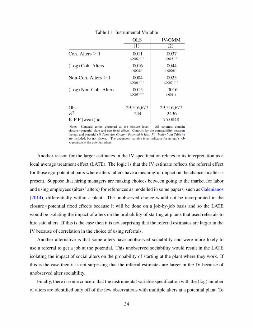
Table 11: Instrumental Variable

OLS IV-GMM(1) (2)

Coh. Alters ≥ 1 .0011 .0037(.0002)∗∗∗ (.0015)∗∗

(Log) Coh. Alters .0016 .0044(.0008)∗ (.0026)∗

Non-Coh. Alters ≥ 1 .0004 .0025(.0001)∗∗∗ (.0007)∗∗∗

(Log) Non-Coh. Alters .0015 -.0016(.0003)∗∗∗ (.0011)

Obs. 29,516,677 29,516,677R2 .244 .2436K-P F (weak) id 75.0848Note: Standard errors clustered at the closure level. All columns contain

closure×potential plant and ego fixed effects. Controls for the compatibility betweenthe ego and potential (% Same Age Group – Potential is Hist. Pl. (Indic) from Table 4)are included, but not shown. The dependent variable is an indicator for an ego’s jobacquisition at the potential plant.

Another reason for the larger estimates in the IV specification relates to its interpretation as a

local average treatment effect (LATE). The logic is that the IV estimate reflects the referral effect

for those ego-potential pairs where alters’ alters have a meaningful impact on the chance an alter is

present. Suppose that hiring managers are making choices between going to the market for labor

and using employees (alters’ alters) for references as modelled in some papers, such as Galenianos

(2014), differentially within a plant. The unobserved choice would not be incorporated in the

closure×potential fixed effects because it will be done on a job-by-job basis and so the LATE

would be isolating the impact of alters on the probability of starting at plants that used referrals to

hire said alters. If this is the case then it is not surprising that the referral estimates are larger in the

IV because of correlation in the choice of using referrals.

Another alternative is that some alters have unobserved sociability and were more likely to

use a referral to get a job at the potential. This unobserved sociability would result in the LATE

isolating the impact of social alters on the probability of starting at the plant where they work. If

this is the case then it is not surprising that the referral estimates are larger in the IV because of

unobserved alter sociability.

Finally, there is some concern that the instrumental variable specification with the (log) number

of alters are identified only off of the few observations with multiple alters at a potential plant. To

34

address this concern Appendix Table D.2 presents the OLS and IV estimates without the (log)

alters variables and it remains consistent with the above results, but this comes at the cost of not

addressing the correlation between the existence of a cohort-alter and the number of alters and

so this is not the preferred specification. The IV results are certainly complements to the main

specification and the consistency with previous results serves as supporting evidence.

7 Conclusion

In this paper, I robustly estimated the impact that a former co-worker has on the chance that an

individual becomes hired at a specific plant. I found that the hiring-cohort effect is larger than

the impact of other non-hiring-cohort connections. The existence of one hiring-cohort co-worker

increases the chance of going to a plant by 3.7-fold which is 2.75 times more than one non-hiring-

cohort co-worker. I also address several biases associated with inferred job referral in the existing

literature and show that results are robust to placebo tests and controlling for selection on unob-

servable characteristics (with a peers-of-peers instrument).

Establishing the existence of a referral effect is the first step toward potential welfare compar-

isons from cohort hiring policies. Future work can study the impact of hiring-cohort workers and

characteristics on the quality of the employment outcomes. For example, previous literature has

looked at the impact of co-worker connections on unemployment duration, turnover and wages

(Cingano and Rosolia 2012, Hensvik and Skans forthcoming, Brown, Setren, and Topa 2016).

The addition of the hiring-cohort analysis to these research agendas and other improvements could

provide a more accurate estimate of the welfare benefits of job referral networks.

35

References

ALTONJI, J. G., AND D. CARD (1991): “The Effects of Immigration on the Labor Market Outcomes of

Less-skilled Natives,” in Immigration, trade and the labor market, pp. 201–234. University of Chicago

Press.

BAUM, C. F., M. E. SCHAFFER, S. STILLMAN, ET AL. (2003): “Instrumental Variables and GMM: Esti-

mation and Testing,” Stata Journal, 3(1), 1–31.

BAYER, P., S. L. ROSS, AND G. TOPA (2008): “Place of Work and Place of Residence: Informal Hiring

Networks and Labor Market Outcomes,” Journal of Political Economy, 116(6), 1150–1196.

BOSCH, M., AND J. ESTEBAN-PRETEL (2012): “Job Creation and Job Destruction in the Presence of

Informal Markets,” Journal of Development Economics, 98(2), 270–286.

BOSCH, M., AND W. F. MALONEY (2010): “Comparative Analysis of Labor Market Dynamics using

Markov Processes: An Application to Informality,” Labour Economics, 17(4), 621–631.

BRAMOULLE, Y., H. DJEBBARI, AND B. FORTIN (2009): “Identification of Peer Effects through Social

Networks,” Journal of Econometrics, 150(1), 41–55.

BROWN, M., E. SETREN, AND G. TOPA (2016): “Do Informal Referrals Lead to Better Matches? Evidence

from a Firms Employee Referral System,” Journal of Labor Economics, 34(1), 161–209.

CHEN-ZION, A., AND J. E. RAUCH (2016): “History Dependence in Networks of Close Relationships:

Theory and evidence from cohort attachment in employee entrepreneurship,” University of California,

San Diego, unpublished manuscript.

CINGANO, F., AND A. ROSOLIA (2012): “People I Know: Job Search and Social Networks,” Journal of

Labor Economics, 30(2), 291–332.

CORREIA, S. (2015): “REGHDFE: Stata module to perform linear or instrumental-variable regression ab-

sorbing any number of high-dimensional fixed effects,” .

DE GIORGI, G., M. PELLIZZARI, AND S. REDAELLI (2010): “Identification of social interactions through

partially overlapping peer groups,” American Economic Journal: Applied Economics, pp. 241–275.

DUSTMANN, C., A. GLITZ, U. SCHONBERG, AND H. BRUECKER (forthcoming): “Referral-based Job

Search Networks,” Review of Economic Studies.

36

FINK, M., E. SEGALLA, A. WEBER, AND C. ZULEHNER (2010): “Extracting firm information from ad-

ministrative records: The ASSD Firm Panel,” Discussion paper, NRN Working Paper, NRN: The Austrian

Center for Labor Economics and the Analysis of the Welfare State.

GALENIANOS, M. (2014): “Hiring Through Referrals,” Journal of Economic Theory, 152, 304–323.

GEE, L. K., J. JONES, AND M. BURKE (forthcoming): “Social Networks and Labor Markets: How Strong

Ties Relate to Job Finding On Facebooks Social Network,” Journal of Labor Economics.

GRANOVETTER, M. (1973): “The Strength of Weak Ties,” American Journal of Sociology, 78(6), 1360–

1380.

(1983): “The Strength of Weak Ties: A Network Theory Revisited,” Sociological Theory, 1(1),

201–233.

(1995): Getting a Job: A Study of Contacts and Careers. University of Chicago Press.

(2005): “The Impact of Social Structure on Economic Outcomes,” The Journal of Economic Per-

spectives, 19(1), 33–50.

HENLEY, A., G. R. ARABSHEIBANI, AND F. G. CARNEIRO (2009): “On Defining and Measuring the

Informal Sector: Evidence from Brazil,” World Development, 37(5), 992–1003.

HENSVIK, L., AND O. N. SKANS (forthcoming): “Social Networks, Employee Selection and Labor Market

Outcomes,” Journal of Labor Economics.

INSTITUTO BRASILERO DE GEOGRAFIA E ESTATISTICA (2001): “Demographic Cen-

sus 2000: Population and Household Characterisitics,” Accessed August 25, 2014

http://www.ibge.gov.br/english/estatistica/populacao/censo2000/default.shtm.

(2011): “2010 Population Census,” Accessed August 25, 2014

http://www.ibge.gov.br/english/estatistica/populacao/censo2010/default.shtm.

IOANNIDES, Y. M., AND L. D. LOURY (2004): “Job Information Networks, Neighborhood Effects, and

Inequality,” Journal of Economic Literature, 42(4), 1056–1093.

JOVANOVIC, B. (1979): “Job Matching and the Theory of Turnover,” The Journal of Political Economy,

87(5), 972–990.

37

KERR, W. R., AND M. MANDORFF (2015): “Social Networks, Ethnicity, and Entrepreneurship,” Working

Paper 21597, National Bureau of Economic Research.

KRAMARZ, F., AND O. N. SKANS (2014): “When Strong Ties are Strong: Networks and Youth Labour

Market Entry,” The Review of Economic Studies, 81(3), 1164–1200.

LUNDEN, I. (2015): “LinkedIn Debuts Referrals, Relaunches Recruiter With People-Matching Algorithms,”

Tech Crunch, October 14, 2015. Accessed October 15, 2015, http://techcrunch.com/2015/10/14/linkedin-

debuts-referrals-relaunches-recruiter-with-people-matching-algorithms/.

MARSDEN, P. V. (1990): “Network Data and Measurement,” Annual Review of Sociology, 16, 435–463.

MCPHERSON, M., L. SMITH-LOVIN, AND J. M. COOK (2001): “Birds of a Feather: Homophily in Social

Networks,” Annual Review of Sociology, 27, 415–444.

MENEZES-FILHO, N. A., M.-A. MUENDLER, AND G. RAMEY (2008): “The Structure of Worker Com-

pensation in Brazil, with a Comparison to France and the United States,” The Review of Economics and

Statistics, 90(2), 324–346.

MUENDLER, M.-A., J. POOLE, G. RAMEY, AND T. WAJNBERG (2004): “Job Concordances for Brazil:

Mapping the Classificacao Brasileira de Ocupacoes (CBO) to the International Standard Classification of

Occupations (ISCO-88),” University of California, San Diego, unpublished manuscript.

MUENDLER, M.-A., AND J. E. RAUCH (2015): “Mobilizing Social Capital Through Employee Spinoffs:

Evidence from Brazil,” University of California, San Diego, unpublished manuscript.

MUENDLER, M.-A., J. E. RAUCH, AND O. TOCOIAN (2012): “Employee Spinoffs and Other Entrants:

Stylized Facts from Brazil,” International Journal of Industrial Organization, 30(5), 447–458.

NORDMAN, C., AND L. PASQUIER-DOUMER (2015): “Transitions in a West African labour market: The

role of family networks,” Journal of Behavioral and Experimental Economics (formerly The Journal of

Socio-Economics), 54(C), 74–85.

PALLAIS, A., AND E. G. SANDS (forthcoming): “Why the Referential Treatment? Evidence from Field

Experiments on Referrals,” Journal of Political Economy.

REES, A. (1966): “Information Networks in Labor Markets,” The American Economic Review, 56(1/2),

559–566.

38

SAYGIN, P. O., A. WEBER, AND M. A. WEYNANDT (2014): “Effect of Past Coworkers on Job Search

Evidence from Austria,” unpublished manuscript.

SCHMUTTE, I. M. (2015): “Job Referral Networks and the Determination of Earnings in Local Labor

Markets,” Journal of Labor Economics, 33(1), 1–32.

SCHWERDT, G. (2011): “Labor Turnover Before Plant Closure: “Leaving the sinking ship” vs. “Captain

throwing ballast overboard”,” Labour Economics, 18(1), 93–101.

THE WORLD BANK WORLD DEVELOPMENT INDICATORS (2014): “Population, total,” [Data file]. Re-

trieved from http://data.worldbank.org/indicator/SP.POP.TOTL.

WOOLDRIDGE, J. M. (2001): Econometric Analysis of Cross Section and Panel Data, vol. 1 of MIT Press

Books. The MIT Press.

ZENGER, T. R., AND B. S. LAWRENCE (1989): “Organizational Demography: The Differential Effects of

Age and Tenure Distributions on Technical Communication,” Academy of Management Journal, 32(2),

353–376.

39

Appendix

A Sample Selection

Table A.1: Selection ComparisonDimension Saygin et al WP This paperClosure

1980-2007 Austria 1998-1999 Brazil (Ceara, Acre,Santa Catarina, Mato Grosso)

do Sul, Espirito Santo)Distinguish Exit by worker-flow approach last year observed in data

(Fink, Segalla, Weber, and Zulehner 2010)Period of Firm Exit Quarter YearMin. Num. Employees in last per. 5 5

EgoBlue or white Males, ≥ 20

collar workers, 20-55 hrs/weekAt closure in the period of firm exit? Not leaving for

death or retirementTenure at closure > 1 yr > 3 monthsAlters - > 1 employed alterRe-employment censored at... 1 yr 2 yrsLocation of re-employment same country as closure same state as closure

Alter? Males, ≥ 20 hrs/week

Time Since last Co-worked ≤ 5 years ≤ 4 yearsOverlap > 30 days > 3 monthsIf.. ego’s hist. firm has ≤ 3000 ego’s plantExcluding.. egos from the same closure alt.+egos from the closure firm

PotentialLocation of alters.. firm in closure qtr. pl. in month ego leaves closureMinimum tenure of alter ? 3 months

40

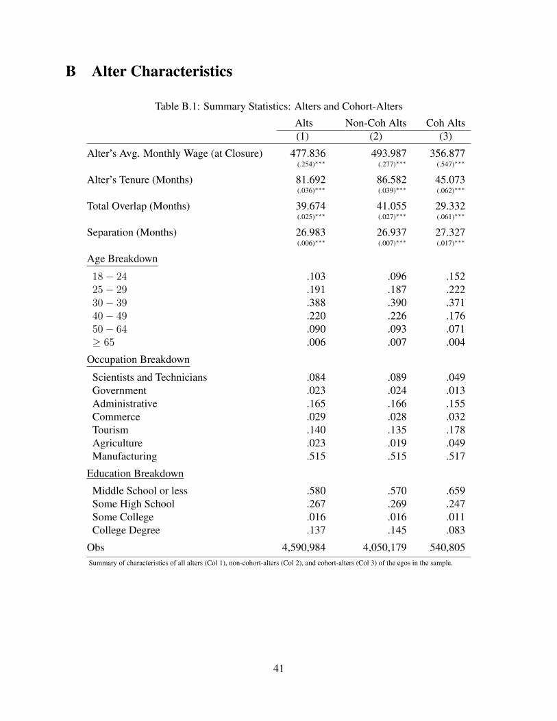
B Alter Characteristics

Table B.1: Summary Statistics: Alters and Cohort-Alters

Alts Non-Coh Alts Coh Alts(1) (2) (3)

Alter’s Avg. Monthly Wage (at Closure) 477.836 493.987 356.877(.254)∗∗∗ (.277)∗∗∗ (.547)∗∗∗

Alter’s Tenure (Months) 81.692 86.582 45.073(.036)∗∗∗ (.039)∗∗∗ (.062)∗∗∗

Total Overlap (Months) 39.674 41.055 29.332(.025)∗∗∗ (.027)∗∗∗ (.061)∗∗∗

Separation (Months) 26.983 26.937 27.327(.006)∗∗∗ (.007)∗∗∗ (.017)∗∗∗

Age Breakdown

18− 24 .103 .096 .15225− 29 .191 .187 .22230− 39 .388 .390 .37140− 49 .220 .226 .17650− 64 .090 .093 .071≥ 65 .006 .007 .004

Occupation Breakdown

Scientists and Technicians .084 .089 .049Government .023 .024 .013Administrative .165 .166 .155Commerce .029 .028 .032Tourism .140 .135 .178Agriculture .023 .019 .049Manufacturing .515 .515 .517

Education Breakdown

Middle School or less .580 .570 .659Some High School .267 .269 .247Some College .016 .016 .011College Degree .137 .145 .083

Obs 4,590,984 4,050,179 540,805Summary of characteristics of all alters (Col 1), non-cohort-alters (Col 2), and cohort-alters (Col 3) of the egos in the sample.

41

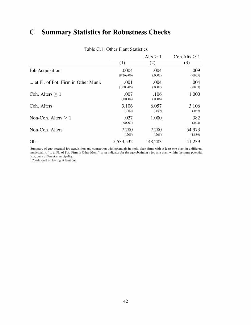
C Summary Statistics for Robustness Checks

Table C.1: Other Plant Statistics

Alts ≥ 1 Coh Alts ≥ 1(1) (2) (3)

Job Acquisition .0004 .004 .009(8.26e-06) (.0002) (.0005)

... at Pl. of Pot. Firm in Other Muni. .001 .004 .004(1.00e-05) (.0002) (.0003)

Coh. Alters ≥ 1 .007 .106 1.000(.00004) (.0008)

Coh. Alters 3.106 6.057 3.106(.062) (.159) (.062)

Non-Coh. Alters ≥ 1 .027 1.000 .382(.00007) (.002)

Non-Coh. Alters 7.280 7.280 54.973(.205) (.205) (1.889)

Obs 5,533,532 148,283 41,239Summary of ego-potential job acquisition and connection with potentials in multi-plant firms with at least one plant in a different

municipality. “... at Pl. of Pot. Firm in Other Muni.” is an indicator for the ego obtaining a job at a plant within the same potentialfirm, but a different municipality.1 Conditional on having at least one.

42

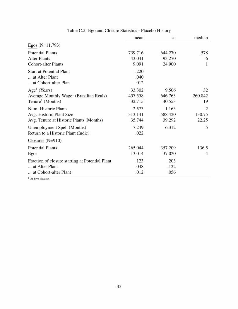
Table C.2: Ego and Closure Statistics - Placebo History

mean sd median

Egos (N=11,793)

Potential Plants 739.716 644.270 578Alter Plants 43.041 93.270 6Cohort-alter Plants 9.091 24.900 1

Start at Potential Plant .220... at Alter Plant .040... at Cohort-alter Plan .012

Age1 (Years) 33.302 9.506 32Average Monthly Wage1 (Brazilian Reals) 457.558 646.763 260.842Tenure1 (Months) 32.715 40.553 19

Num. Historic Plants 2.573 1.163 2Avg. Historic Plant Size 313.141 588.420 130.75Avg. Tenure at Historic Plants (Months) 35.744 39.292 22.25

Unemployment Spell (Months) 7.249 6.312 5Return to a Historic Plant (Indic) .022

Closures (N=910)

Potential Plants 265.044 357.209 136.5Egos 13.014 37.020 4

Fraction of closure starting at Potential Plant .123 .203... at Alter Plant .048 .122... at Cohort-alter Plant .012 .0561 At firm closure.

43

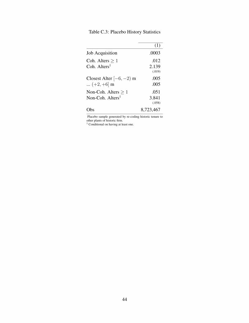
Table C.3: Placebo History Statistics

(1)

Job Acquisition .0003

Coh. Alters ≥ 1 .012Coh. Alters1 2.139

(.019)

Closest Alter [−6,−2) m .005... (+2,+6] m .005

Non-Coh. Alters ≥ 1 .051Non-Coh. Alters1 3.841

(.058)

Obs 8,723,467Placebo sample generated by re-coding historic tenure to

other plants of historic firm.1 Conditional on having at least one.

44

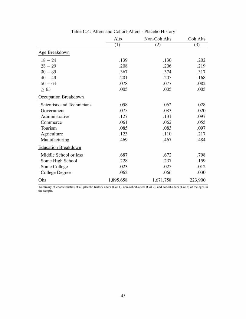
Table C.4: Alters and Cohort-Alters - Placebo History

Alts Non-Coh Alts Coh Alts(1) (2) (3)

Age Breakdown

18− 24 .139 .130 .20225− 29 .208 .206 .21930− 39 .367 .374 .31740− 49 .201 .205 .16850− 64 .078 .077 .082≥ 65 .005 .005 .005

Occupation Breakdown

Scientists and Technicians .058 .062 .028Government .075 .083 .020Administrative .127 .131 .097Commerce .061 .062 .055Tourism .085 .083 .097Agriculture .123 .110 .217Manufacturing .469 .467 .484

Education Breakdown

Middle School or less .687 .672 .798Some High School .228 .237 .159Some College .023 .025 .012College Degree .062 .066 .030

Obs 1,895,658 1,671,758 223,900Summary of characteristics of all placebo history alters (Col 1), non-cohort-alters (Col 2), and cohort-alters (Col 3) of the egos in

the sample.

45

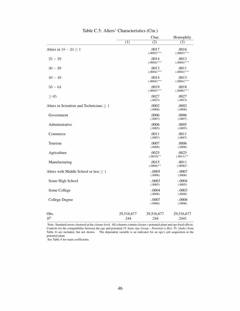
Table C.5: Alters’ Characteristics (Ctn.)Char. Homophily

(1) (2) (3)

Alters in 18− 24 ≥ 1 .0017 .0016(.0005)∗∗∗ (.0005)∗∗∗

25− 29 .0014 .0013(.0004)∗∗∗ (.0004)∗∗∗

30− 39 .0013 .0011(.0004)∗∗∗ (.0004)∗∗∗

40− 49 .0014 .0013(.0004)∗∗∗ (.0004)∗∗∗

50− 64 .0019 .0018(.0005)∗∗∗ (.0006)∗∗∗

≥ 65 .0027 .0027(.0023) (.0023)

Alters in Scientists and Technicians ≥ 1 .0002 .0002(.0006) (.0006)

Government .0006 .0006(.0007) (.0007)

Administrative .0006 .0005(.0005) (.0005)

Commerce .0011 .0011(.0007) (.0007)

Tourism .0007 .0006(.0006) (.0006)

Agriculture .0025 .0025(.0010)∗∗ (.0011)∗∗

Manufacturing .0015 .0011(.0006)∗∗ (.0006)∗

Alters with Middle School or less ≥ 1 -.0005 -.0007(.0006) (.0006)

Some High School -.0003 -.0004(.0005) (.0005)

Some College -.0004 -.0003(.0008) (.0008)

College Degree -.0007 -.0008(.0006) (.0006)

Obs. 29,516,677 29,516,677 29,516,677R2 .244 .244 .2441

Note: Standard errors clustered at the closure level. All columns contain closure×potential plant and ego fixed effects.Controls for the compatibility between the ego and potential (% Same Age Group – Potential is Hist. Pl. (Indic) fromTable 4) are included, but not shown. The dependent variable is an indicator for an ego’s job acquisition at thepotential plant.See Table 8 for main coefficients.

46

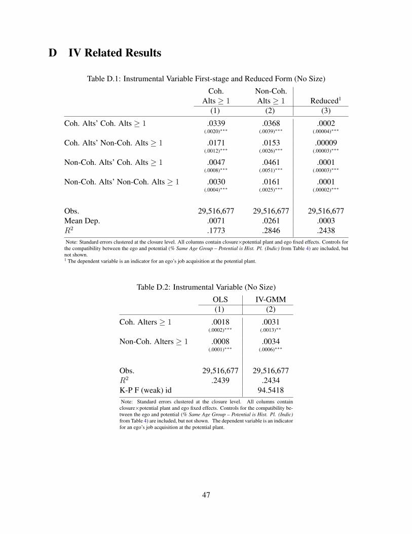
D IV Related Results

Table D.1: Instrumental Variable First-stage and Reduced Form (No Size)

Coh. Non-Coh.Alts ≥ 1 Alts ≥ 1 Reduced1

(1) (2) (3)

Coh. Alts’ Coh. Alts ≥ 1 .0339 .0368 .0002(.0020)∗∗∗ (.0039)∗∗∗ (.00004)∗∗∗

Coh. Alts’ Non-Coh. Alts ≥ 1 .0171 .0153 .00009(.0012)∗∗∗ (.0026)∗∗∗ (.00003)∗∗∗

Non-Coh. Alts’ Coh. Alts ≥ 1 .0047 .0461 .0001(.0008)∗∗∗ (.0051)∗∗∗ (.00003)∗∗∗

Non-Coh. Alts’ Non-Coh. Alts ≥ 1 .0030 .0161 .0001(.0004)∗∗∗ (.0025)∗∗∗ (.00002)∗∗∗

Obs. 29,516,677 29,516,677 29,516,677Mean Dep. .0071 .0261 .0003R2 .1773 .2846 .2438Note: Standard errors clustered at the closure level. All columns contain closure×potential plant and ego fixed effects. Controls for

the compatibility between the ego and potential (% Same Age Group – Potential is Hist. Pl. (Indic) from Table 4) are included, butnot shown.1 The dependent variable is an indicator for an ego’s job acquisition at the potential plant.

Table D.2: Instrumental Variable (No Size)

OLS IV-GMM(1) (2)

Coh. Alters ≥ 1 .0018 .0031(.0002)∗∗∗ (.0013)∗∗

Non-Coh. Alters ≥ 1 .0008 .0034(.0001)∗∗∗ (.0006)∗∗∗

Obs. 29,516,677 29,516,677R2 .2439 .2434K-P F (weak) id 94.5418Note: Standard errors clustered at the closure level. All columns contain

closure×potential plant and ego fixed effects. Controls for the compatibility be-tween the ego and potential (% Same Age Group – Potential is Hist. Pl. (Indic)from Table 4) are included, but not shown. The dependent variable is an indicatorfor an ego’s job acquisition at the potential plant.

47

E Maps

Figure E.1: Brazilian State Coverage - Source: Brazil. Map. Google Maps. 17 August 2014.

48

Figure E.2: Distribution of Urban Population 2000 - Source: IBGE 2000

49

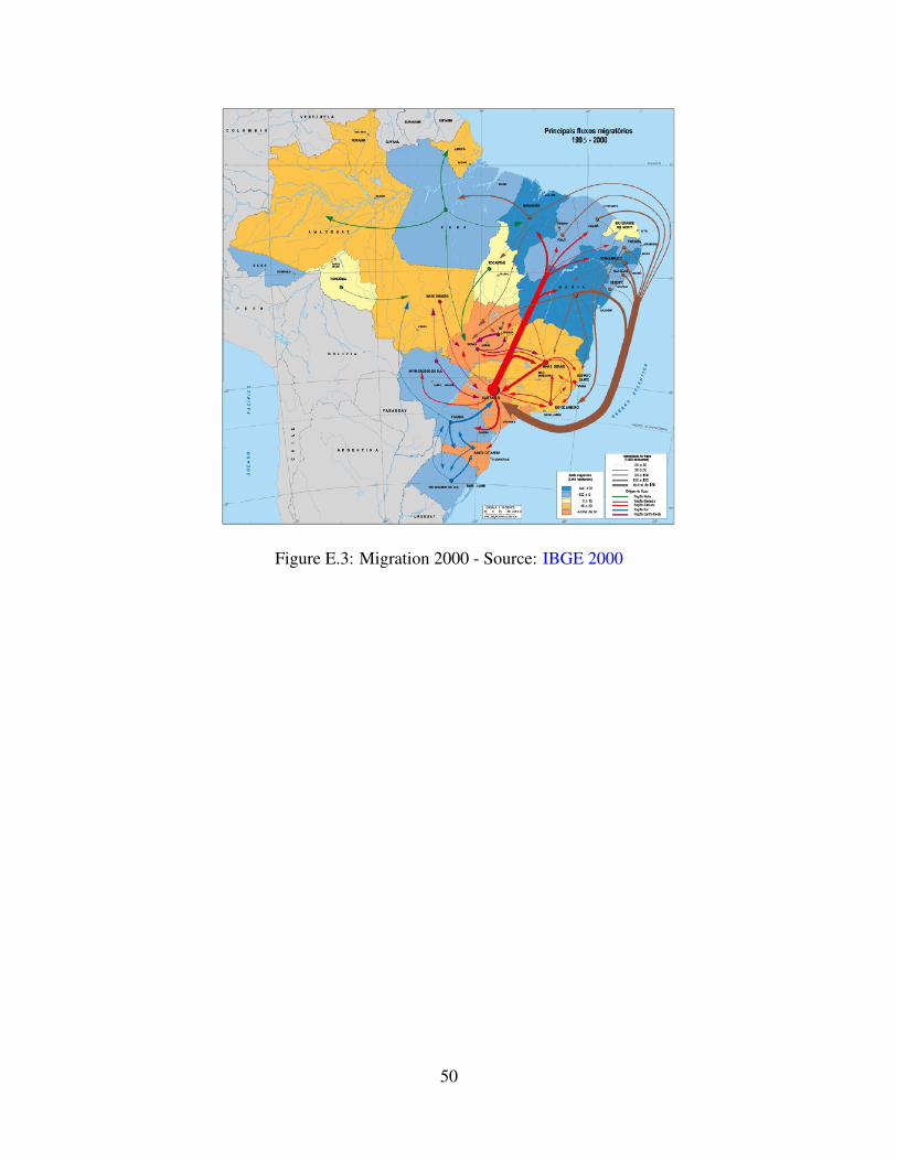
Figure E.3: Migration 2000 - Source: IBGE 2000

50