The Attractive Traveling Salesman Problem

Gunes Erdogan ∗,† Jean-Francois Cordeau ∗ Gilbert Laporte †

August 14, 2007

Abstract

In the Attractive Traveling Salesman Problem the vertex set is partitioned

into facility vertices and customer vertices. A maximum profit tour must be

constructed on a subset of the facility vertices. Profit is computed through an

attraction function: every visited facility vertex attracts a portion of the profit

from the customer vertices based on the distance between the facility and cus-

tomer vertices, and the attractiveness of the facility vertex. A gravity model

is used for computing the profit attraction. The problem is formulated as an

integer non-linear program. A linearization is proposed and is strengthened

through the introduction of valid inequalities, and a branch-and-cut algorithm

is developed. A tabu search algorithm is also implemented. Computational

results are reported.

Keywords: traveling salesman problem, demand attraction, demand alloca-

tion, linearization, branch-and-cut, tabu search.

1 Introduction

The purpose of this paper is to introduce a new variant of the Traveling Salesman

Problem (TSP), called the Attractive Traveling Salesman Problem (ATSP). TheATSP is defined on an undirected graph G = (V ∪W, E), where V ∪W is the vertex

∗Canada Research Chair in Logistics and Transportation, HEC Montreal, 3000 Chemin de la

Cote-Sainte-Catherine, Montreal, Canada H3T 2A7†Canada Research Chair in Distribution Management, HEC Montreal, 3000 Chemin de la Cote-

Sainte-Catherine, Montreal, Canada H3T 2A7

1

set and E = {(vi, vj) : vi, vj ∈ V ∪ W, i < j} is the edge set. The set V is a set offacility vertices, while the set W is a set of customer vertices. Let T be a subset ofcompulsory vertices of V , including a depot v0. A distance dij and a travel time tijare associated with each edge (vi, vj). A profit pk is associated with each customervertex vk. Each facility vertex vi on the tour, apart from the depot, generates a profitderived from the customer vertices, which is measured by an attraction function tobe defined later. Including vertex vi in the cycle generates a dwell time ri. The cyclelength, including travel and dwell times, may not exceed an upper limit L. The aimof the ATSP is to design a cycle or tour of maximal profit, including all vertices ofT and possibly some vertices of V \ T , subject to the length constraint.

An application of the ATSP arises in the planning of a tour of a mobile enter-tainment facility such as a circus or a theater company. The amount of time thatcan be spent by the mobile facility is limited. Visiting a facility vertex generates aprofit. Facilities with extra services and closer to the larger population centers areassumed to be more attractive from the customers’ point of view, and consequentlyvisiting these facilities is more profitable. Another application arises in the routingof a military reconnaissance vehicle. In this application, the customer sites are theenemy installations or encampments, the facility sites are the possible observationpoints, and the travel distance limit is dictated by either the fuel capacity or theallowed duration of the mission. The attractiveness of a candidate observation pointmay be perceived as a function of its visibility range and concealment factor. Theobjective function becomes the maximization of information gathered. Yet anotherapplication is the design of a route for a mobile health care facility operating in anunderdeveloped region. Typically, such a facility can only visit a subset of locali-ties accessible by the main road network. Population centers located outside theselocalities access them on foot. The accessibility problem is exacerbated during therainy seasons when only paved roads can be used by the mobile facility (Oppongand Hodgson, 1994; Hodgson, Laporte, and Semet, 1998).

There exist many studies on Traveling Salesman Problems with Profits. A recentsurvey by Feillet, Dejax, and Gendreau (2005) lists 95 references. This survey cat-egorizes the problems into three classes, based on how the objectives of minimizingdistance and maximizing profit are handled. The first class consists of problems inwhich both of the objectives are combined in the objective function. The secondclass is composed of problems in which the travel cost is a constraint and the objec-tive is to maximize the profits collected. Finally, the problems in which the profit is aconstraint and the objective is to minimize the travel cost constitute the third class.According to this categorization our problem is closest to the problems in the second

2

class, together with the Orienteering Problem (Golden, Levy, and Vohra, 1987), theMaximum Collection Problem (Kataoka and Morito, 1988), and the Selective Trav-

eling Salesman Problem (Laporte and Martello, 1990). The most successful exactstudy regarding this class of problems is the one by Fischetti, Salazar Gonzalez, andToth (1998), in which the authors were able to solve instances involving up to 500vertices within a few hours, using a branch-and-cut algorithm. The most successfulheuristic for this class of problems is due to Gendreau, Laporte, and Semet (1998).These authors use a tabu search algorithm to solve instances involving up to 300vertices in a few minutes, with an optimality gap typically less than 1%.

In all these studies profits are assumed to be collected from the visited vertices,implicitly implying that customer and facility vertices coincide, which may not bethe case in all applications. As an example from the entertainment sector, racetracks are usually built outside the urban centers to avoid the noise and pollutiongenerated by these facilities. Similarly, ski slopes are located in the mountainousareas, which are usually at a significant distance from the major population centers.In our study, we assume that the facility vertices and customer vertices do notcoincide, although they can be arbitrarily close. This distinction also allows thedivision of the demand of a population center into smaller parts located around thefacility, thereby permitting a finer aggregation of the demand data.

Because the sets of customer and facility vertices are disjoint, the questions ofhow much demand is captured and how the captured demand is allocated to facilitiesarise. To the best of our knowledge these questions have not been fully addressed inthe literature on routing, perhaps because customer and facility vertices are usuallynot separated. There are a few notable exceptions. In Lee, Chiu, and Sanchez(1998), the authors define and study the Steiner Ring Star Problem, in which atour over a subset of the facility vertices must be determined; the demand of acustomer vertex is assumed to be assigned to the closest visited facility vertex. Theobjective is to minimize the sum of travel and assignment costs. In two closelyrelated studies by Labbe, Laporte, Rodriguez-Martın, and Salazar Gonzalez (2004,2005), the authors solve the Ring Star Problem and the Median Cycle Problem. Thedifference between the problem studied in the former paper and the Steiner RingStar Problem is that there is no distinction between facility and customer vertices,and each vertex can be visited. In the Median Cycle Problem, the objective is tominimize the routing cost, and there is an upper bound on the assignment cost.Another exception is the set of problems with covering aspect, such as the Covering

Tour Problem introduced by Current in 1981, where a customer vertex is covered ifit is within a prespecified distance of a visited facility vertex, and all the demand of

3

a customer vertex is assumed to be attracted to the visited facility vertices withinthe coverage range.

Demand attraction and allocation functions have been studied in the compet-itive location literature. The reader is referred to Drezner (1995) for a survey ofcompetitive facility location models, and to Eiselt and Laporte (1998) for a criticalreview of demand allocation functions. It has been suggested by Hotelling (1929)that each customer patronizes the closest facility in a winner-takes-all manner, giventhat prices are identical. Much later, based on the gravity model of Reilly (1931),Huff (1964, 1966) has used a gravity function by which the probability Pki that acustomer at vk patronizes a given facility vi is proportional to the attractivenessof the facility, and inversely proportional to some power of the distance betweenthe customer and the facility. In subsequent work, Hodgson (1981) has advocatedusing an exponential distance decay function rather than a polynomial one. Dreznerand Drezner (2002) have tested and validated Huff’s gravity based model using realworld data, both for the polynomial and the exponential distance decay functions.One of the authors’ conclusions is that the results are not sensitive to the choice ofthe distance decay function. The gravity based model has been used in the studiesby Jain and Mahajan (1979), Drezner (1994), Bell, Ho, and Tang (1998), and morerecently by Drezner and Drezner (2004, 2006, and 2007). Encouraged by these stud-ies, we have chosen the gravity based model for determining the demand attractionand allocation.

The remainder of the paper is organized as follows. In Section 2, we provide adefinition of the attraction function, we formally define the problem, we present aproof of NP-hardness, and we introduce a non-linear formulation. In Section 3, wepropose a linearization scheme involving an infinite number of potential constraints,as well as valid inequalities. We describe a branch-and-cut algorithm for the problemin Section 4, and a tabu search algorithm in Section 5. Computational results forboth the branch-and-cut and tabu search algorithms are presented in Section 6. InSection 7, we analyze an extension of the problem where there may be more thanone option of service at the facility vertices. Conclusions follow in Section 8.

2 The Model

Based on Huff’s gravity function, we derive a general formula for the probability Pki

that a customer from vertex vk patronizes a facility at vertex vi:

4

Pki =

ai

dqki∑

vj∈V \{v0}

aj

dqkj

, (1)

where ai is the attractiveness of the facility at vertex vi, and q ≥ 1 is a parameter.The attractiveness ai of vertex vi is based on the size, services, and other factorsrelated to that facility.

One shortcoming of the demand attraction function (1) is the assumption thatdemand is never lost. In reality, some customers may choose not to get the servicebecause substitute services are more attractive, or the visited facility vertices aretoo far away to be reached conveniently. To cope with this problem, we apply aminor modification to (1). Let bk be the self-attraction of customer vertex vk. Thenthe formula becomes:

Pki =

ai

dqki

bk +∑

vj∈V \{v0}

aj

dqkj

. (2)

An interpretation of bk is an estimate of substitute services available for vertex vk.

While this modified allocation function suits our purposes better, it also violatesthe principle of insensitivity to scaling (Eiselt and Laporte, 1998) because of theconstant in the denominator. That is, any scaling change in the distance or theattractiveness measurement will change the demand allocation. A simple way toovercome this problem is to redefine all parameters as the result of the division of theoriginal parameters by its minimum, i.e. dij := dij/min{dkl|vk, vl ∈ V ∪W, vk 6= vl},ai := ai/min{aj|vj ∈ V \{v0}} and modify the estimates for all bk values accordingly.

We now prove that ATSP is NP-hard by a reduction from the Selective TravelingSalesman Problem.

Selective Traveling Salesman Problem (STSP): Given a graph G = (V, E), aset T ⊂ V of compulsory vertices, a distance dij associated with every edge in E, alimit on the total distance traveled L, and a positive integer profit pi associated witheach vertex in V , determine a maximal profit cycle whose length does not exceed L.STSP was proved to be NP-hard by Laporte and Martello (1990).

Proposition 1. ATSP is NP-hard.

5

Proof: We construct a reduction from the recognition form of the STSP. Take anarbitrary instance of the STSP. The recognition form of STSP is the question ofthe existence of a solution with objective function value greater than or equal toK. Construct an instance of the ATSP by adding a single customer vertex vs, atan arbitrary distance dis from every vertex vi ∈ V , with a total profit of 1, and aself-attraction value of 1, i.e., W = {vs}, ps = 1, bs = 1. Set the attractivenessof each vertex facility vi ∈ V to ai = pid

qis. Let tij = dij, ri = 0. This setting of

parameters results in an objective function f(x)/(f(x) + 1) for the ATSP, wheref(x) is the objective function of the STSP. Since f(x) ≥ 0, clearly f(x) ≥ K if andonly if f(x)/(f(x) + 1) ≥ K/(K + 1). Solving this instance of the ATSP amountsto solving the STSP instance at hand, so ATSP is at least as hard as STSP. �

We conclude this section by giving a non-linear integer programming formulationof the ATSP. Let xij (i < j) be equal to 1 if the vehicle traverses edge (i, j) and0 otherwise, and let yi be equal to 1 if vertex i is visited and 0 otherwise. Theformulation is as follows:

(ATSP1)

maximize∑

vk∈W

pk

∑

vi∈V \{v0}

Pik =∑

vk∈W

pk

∑

vi∈V \{v0}

ai

dqki

yi

bk +∑

vj∈V \{v0}

aj

dqkj

yj

(3)

subject to

∑

vi∈V,i<j

xij +∑

vi∈V,i>j

xji = 2yj (vj ∈ V ) (4)

∑

vi∈S,vj∈V \Sor vi∈V \S,vj∈V

xij ≥ 2yt (S ⊂ V : 2 ≤ |S| ≤ |V | − 2, T \ S 6= ∅, vt ∈ S) (5)

∑

vi,vj∈V

tijxij +∑

vi∈V

riyi ≤ L (6)

yi = 1 (vi ∈ T ) (7)

yi = 0 or 1 (vi ∈ V \ T ) (8)

xij = 0 or 1 ((vi, vj) ∈ E). (9)

6

The objective function (3) maximizes the profit generated from the customervertices. Constraints (4) are degree constraints, and constraints (5) are connectivityconstraints (Gendreau, Laporte, and Semet, 1997). Constraints (6) impose a maxi-mal tour duration, while constraints (7) state that all vertices of T must be visited.Other integrality constraints are defined by (8) and (9).

3 Linearization Scheme and Valid Inequalities

In ATSP1, the objective function (3) consists of the sum of |W |(|V | − 1) ratios oflinear functions. This brings the problem into the domain of fractional program-ming, the elements of which are continuous optimization problems with sums of oneor more ratios of functions. For a comprehensive survey of algorithms and literatureon fractional programming, we refer to reader to Schaible (1995, 1996), Freund andJarre (2001), and Benson (2004). The case of a single ratio of two linear functionsand a polyhedron of feasible solutions is well solved, and can be handled throughlinear programming methods. However, the general fractional programming prob-lem with more than a single ratio (also known as the sum-of-ratios problem) remainshard. It has been shown by Freund and Jarre (2001) that the sum-of-ratios prob-lem is NP-complete. Most available algorithms for fractional programming withmultiple ratios are based on sophisticated non-linear optimization algorithms, or onbranch-and-bound. However, ATSP is a particular discrete optimization problemand standard methods are too time consuming to be used for solving the subprob-lems.

We first show that our problem possesses a special structure, which gives way toa relatively simple linearization scheme using valid inequalities. To the best of ourknowledge linearizing fractional programming problems using valid inequalities is anew idea.

Notice that all terms in the second summation in (3) have the same denominator,allowing us to rewrite it as:

maximize∑

vk∈W

pk

∑

vi∈V \{v0}

ai

dqki

yi

bk +∑

vi∈V \{v0}

ai

dqki

yi

. (10)

7

Let wk =∑

vi∈V \{v0}

ai

dqki

yi, so that (10) simplifies to

maximize∑

vk∈W

pk

wk

bk + wk

. (11)

Each of the functions fk(wk) = wk/(bk + wk) is concave in wk for wk > −bk andcan be approximated by an upper envelope consisting of linear tangents. Formally,at point w∗

k:

fk(wk) =wk

bk + wk

≤bkwk

(bk + w∗k)

2+ (

w∗k

bk + w∗k

−bkw

∗k

(bk + w∗k)

2)

=bkwk

(bk + w∗k)

2+

(w∗k)

2

(bk + w∗k)

2. (12)

Let zk denote the percent of profit captured from customer vertex vk, i.e. zk =wk/(bk + wk), and let y∗ be the vector of y∗

i variables yielding w∗k. Rewriting (12) in

terms of zk, wk, and bk gives

zk ≤

bk(∑

vi∈V \{v0}

ai

dqki

yi)

(bk +∑

vi∈V \{v0}

ai

dqki

y∗i )

2+

(∑

vi∈V \{v0}

ai

dqki

y∗i )

2

(bk +∑

vi∈V \{v0}

ai

dqki

y∗i )

2. (13)

These constraints will be referred to as the linearization constraints. Using thesame reasoning, this idea can be generalized and formalized as follows:

Proposition 2. Let x ∈ X ⊆ Rn, a ∈ Rn, and b, c, d, e, f ∈ R. Define g(x) =(c(ax + b) + d)/(e(ax + b) + f). If −2(cf − ed)/(e(ax + b) + f)3 ≤ 0, ∀x ∈ X, thenthe following inequality is valid ∀x∗ ∈ X:

g(x) ≤(cf − ed)(ax + b)

(e(ax + b) + f)2+

c(ax∗ + b) + d

e(ax∗ + b) + f−

(cf − ed)(ax∗ + b)

(e(ax∗ + b) + f)2. (14)

We can now state our linearization:

(ATSP2)

maximize∑

vk∈W

pkzk (15)

8

subject to0 ≤ zk ≤ 1 (vk ∈ W ). (16)

and (4), (5), (6), (7), (8), (9), (13).

ATSP2 may be strengthened through the introduction of certain valid inequali-ties proposed for the Covering Tour Problem (Gendreau, Laporte, and Semet, 1997).The proofs of validity are identical for both problems.

1) Arc-vertex constraints :

Proposition 3. The inequalities

xij ≤ yi (vi, vj ∈ V ) (17)

and

xij ≤ yj (vi, vj ∈ V ) (18)

are valid for ATSP2.

2) Strong connectivity constraints :

Proposition 4. The inequalities

∑

vi∈S,vj∈V \Sor vi∈V \S,vj∈V

xij ≥ 2 (S ⊂ V : 2 ≤ |S| ≤ |V | − 2, T \ S 6= ∅, S ∩ T 6= ∅) (19)

are valid for ATSP2.

3) Strong 2-matching constraints :

Proposition 5. The following inequalities are valid for ATSP2:

∑

vi,vj∈H

xij +∑

vi,vj∈E′

xij ≤∑

vi∈H

yi +1

2(|E ′ − 1|), (20)

for all H ⊂ V and E ′ ⊂ E satisfying

(i) |{vi, vj} ∩ H| = 1 ((vi, vj) ∈ E ′),

(ii) {vi, vj} ∩ {vk, vl} = ∅ ((vi, vj) 6= (vk, vl) ∈ E ′),

(iii) |E ′| ≥ 3 and odd.

9

4 Branch-and-Cut Algorithm

We now describe a branch-and-cut algorithm using the linearization scheme andvalid inequalities just introduced.

Step 1 (Lower bound). Compute a lower bound z on the optimal solution of theproblem, using a heuristic.

Step 2 (Root node). Construct the linear relaxation of ATSP2 without theconnectivity constraints and the linearization constraints. Insert this subproblem ina list.

Step 3 (Node selection). If the list is empty, stop. Else select and remove asubproblem form the list according to a best-first criterion.

Step 4 (Subproblem solution). Solve the subproblem. Let z∗ be the objectivefunction value, and let x∗, y∗ be the vector values taken by the x and y variables.If z∗ ≤ z, go to Step 3.

Step 5 (Constraint generation). Generate all identified violated connectiv-ity constraints, linearization constraints, arc-vertex constraints, strong connectivityconstraints, and strong 2-matching constraints, and add them to the subproblem.If at least one constraint is generated, go to Step 4.

Step 6 (Integrality check). If the solution is integer, set z = z∗, and go to Step3.

Step 7 (Branching). Construct two subproblems by branching on a binary frac-tional variable with the highest pseudo-cost (Gauthier and Ribiere, 1977). Add thesubproblems to the list and go to Step 3.

The algorithm is handled by CPLEX, except for Step 5. The separation algo-rithms for the constraints to be added during the branch-and-cut algorithm are nowoutlined.

Linearization constraints: Although there are infinitely many members of thisconstraint set, any violated member can be identified in O(|W ||V |) time by simplyplugging in the y∗ and z∗ values. This procedure is equivalent to generating thelinear tangent at the current fractional point.

Arc-vertex constraints: Violated elements of this valid inequality set can beidentified straightforwardly in O(|V |2) time.

Connectivity constraints: Violated members of the connectivity constraints canbe identified by solving a Maximum Flow Problem from each vi ∈ T to each vj ∈V \T , on a network where the upper bounds on the flows are given by the x∗ values.

10

If the maximum flow is less than 2y∗j , then a violated inequality has been identified

along the sets S and T separated by the minimum cut. The complexity of thisprocedure is O(|T ||V |2|E|2), assuming the Maximum Flow Problem is solved by theEdmonds-Karp algorithm (1972).

Strong connectivity constraints: Violated members of the strong connectivityconstraints can be identified by solving a Maximum Flow Problem for each pairof elements from |T |, in O(|T |2|V ||E|2) time with the Edmonds-Karp algorithm.We solve a Maximum Flow Problem for each consecutive pair of vertices from anyordering of the elements of T , which reduces the complexity to O(|T ||V ||E|2) anddoes not result in a significant loss of quality in the lower bound.

Strong 2-matching constraints: To identify the violated strong 2-matching in-equalities, we use the heuristic of Padberg and Rinaldi (1990). We first identifyall blocks of the graph induced by the fractional flow variables. We then take eachblock to be H and try to find a violated inequality by adding edges to E ′, whichhave an endpoint in H and another in V \ H , in a greedy manner.

5 Tabu Search Heuristic

Although the linearization scheme presented in the previous section gives way toa branch-and-cut algorithm, we find it necessary to devise a heuristic for the largeinstances that may exceed the memory and computing time requirements. We nowgive the outline of our tabu search heuristic for ATSP.

We define the insertion neighborhood to be the set of vertices not included inthe tour. The deletion neighborhood is defined as the set of vertices included in thetour but not in the tabu list.

Parameters:

κ : Number of iterations since the last update of the best solution value.

η : The maximum number of iterations without updating the best solution.

λ : A parameter for determining the frequency of diversification.

θ : The number of iterations a vertex stays in the tabu list.

Step 1 (Initialization). Construct a random sequence of the vertices in T \ {v0},and append {v0} to the beginning and end of the sequence to construct a tour.Resequence the tour with the GENIUS algorithm of Gendreau, Hertz, and Laporte(1992) to minimize the total travel time. If the this time is larger than L, stop: the

11

algorithm has failed to find any feasible solution. Else, record the tour as the bestsolution. Set κ = 1.

Step 2 (Search type). If κ = η, stop. Else if κ is a multiple of λθ go to Step 5.

Step 3 (Local search – insertion). For every vertex v in the insertion neighbor-hood, try to insert v in the tour and resequence the tour to minimize the total traveltime. If the tour is feasible and has a solution value higher than the best solution,replace the best solution with the tour at hand, and set κ = 1. If v is not an elementof the tabu list, the tour is feasible, and has a solution value higher than the bestcandidate, set v as the best insertion candidate. Insert the best insertion candidatein the tour, add it to the tabu list, and go to Step 6. If no such candidate is found,go to Step 4.

Step 4 (Local search – deletion). For every vertex v in the deletion neighborhoodand not in the tabu list, try to delete v from the tour and resequence the tour tominimize the total travel time. If the resulting tour is feasible, and has a solutionvalue higher than the best candidate, set v as the best deletion candidate. Deletethe best deletion candidate from the tour, add it to the tabu list, and go to Step 6.

Step 5 (Diversification). Sort the elements v ∈ V \ T that are not in the tourin ascending number of times each element has been added to the tour. For eachelement v in the sorted list, insert v in the tour and resequence the tour to minimizethe total travel time. If the tour is feasible, add v to the tabu list, and go to Step 6.If no insertions are possible, identify a vertex v ∈ V \ T in the tour that has beenremoved from the tour the least number of times. Remove v from the tour, add v tothe tabu list, resequence the tour to minimize the total travel time, and go to Step6.

Step 6 (Tabu list update). Increase the tabu tenure of each vertex in the tabulist by one. Remove from the tabu list the vertices having a tabu tenure greaterthan or equal to θ . Increase κ by 1. Go to Step 2.

6 Computational Results

We have implemented a branch-and-cut algorithm based on ATSP2 and on the validinequalities presented in Propositions 3, 4, and 5. The algorithm was implementedusing CPLEX 10.0.1 on a workstation with a 3.0 Ghz CPU and 1 GB of RAM.We have used q = 2 in (2). We have attempted to solve three sets of randomlycreated problem instances for |V | = 50, 100, and 150. For each instance set, varying

12

values of |W | and |T | were imposed to analyze the effect of these parameters on theperformance of the algorithm. Five instances for each setting have been created,resulting in a total of 180 instances. A computing time limit of one hour wasimposed on the solution of any instance. The results are given in Tables 1, 2, and3, respectively. The column headings are defined as follows:

Succ. : Number of instances successfully solved to optimality.

Avg. Dev. : Average deviation of the best solution found from the best upperbound.

Max. Dev. : Maximum deviation of the best solution found from the best upperbound.

Linearization : Average number of linearization constraints added.

Arc-vertex : Average number of arc-vertex constraints added.

Str. Conn. : Average number of strong connectivity constraints added.

Str. 2-Match : Average number of strong 2-matching constraints added.

Nodes : Average number of nodes generated in the branch-and-cut tree.

Tour size : Average number of vertices included in the best solution found.

Seconds : Average CPU time in seconds.

Opt. : Optimal objective function value.

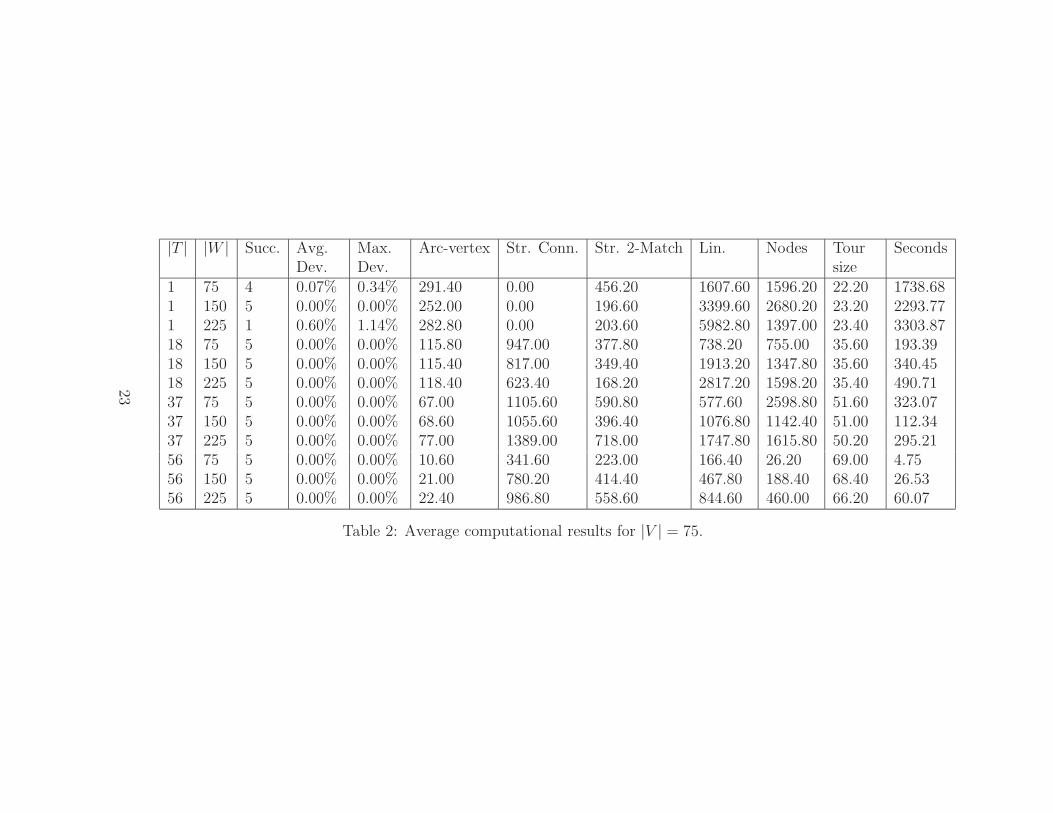
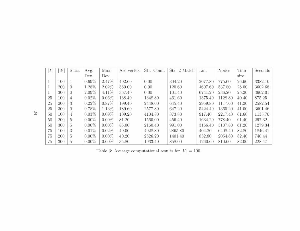
Computational results presented in Tables 1, 2 and 3 offer insights in the internalmechanics of the problem. As expected, the number of linearization constraintsincreases with |W |. The number of arc-vertex inequalities decreases as |T | increases,suggesting that the underlying LP cannot exploit the fractional variables for largevalues of |T |. Another conclusion we can draw from the tables is that the problemis harder for lower values of |T |. This can be explained by the fact that fewer yi

variables are fixed when |T | is small and by the increase in the number of strongconnectivity constraints. We note that CPLEX generated few cover and generalizedupper bound cover inequalities. Finally, the problem is harder for smaller values ofoptimal tour size, and hence smaller values of L. This can be explained as follows.First observe that the slope of the curve in Figure 1 is larger in the region closer to theorigin. This implies that even small changes in the value of wk in this interval causeimportant changes in the overall objective function value. Hence, the underlying LPhas more opportunities to exploit the fractional variables. As wk increases beyonda certain point, the marginal changes do not affect the overall objective functionvalue, and the problem becomes easier.

13

To ensure the repeatability of our results, we have also conducted experiments oninstances adapted from TSPLIB (Reinelt, 1991). We have used the following schemeto convert the data for our problem. We take the first vertex in the data file to bethe depot. We designate the next |T | − 1 vertices together with the first vertex toconstitute T . The next |V |−|T | vertices are used as elements of V \T . The remainingvertices are the elements of W . The attractiveness values of the facility vertices andthe profit values of the customer vertices are computed as (⌊X + Y ⌋mod100) +1. Let Xmax, Xmin, Ymax, Ymin denote the maximum X coordinate, minimum Xcoordinate, maximum Y coordinate, and minimum Y coordinate of all vertices,respectively. We compute dij using the Euclidean distance formula, and set tij = dij,ri = (Xmax − Xmin + Ymax − Ymin)/10 for all vi ∈ V , and L = r|T | + 2.5(Xmax −Xmin + Ymax − Ymin). The self-attraction value of each customer vertex is set to thevalue that will ensure that 70% of the profit is captured if only the closest facilityvertex is visited. The results of the instance files constructed in this manner arepresented in Table 4.

We have also implemented the tabu search heuristic described in Section 5. Inour computational experiments, we have set the tabu tenure limit θ to 10, thediversification parameter λ to 3, and the iteration limit η to 300. The results ofthis algorithm are given in Table 5. Note that in all of the 180 instances tested, theoverall maximum deviation from the upper bound is about 3.25% and the overallaverage deviation is 0.28%. The computing times were no more than four minutes.We have also applied the tabu search algorithm to the instances adapted from theTSPLIB. The longest of those runs took about 15 seconds. The maximum deviationwas 0.74% and the average deviation was 0.04%. We were able to find an optimalsolution in 31 out of the 36 instances.

7 Extension: More Than One Service Option

In closing, we define an interesting extension of the ATSP. In real world applications,there may be more than one option for visiting a facility vertex. These options maydiffer in service time length and the attractiveness values they yield. For example,a circus may be given the opportunity to select a stay of one week or two weeksat a certain facility. In the military example, the reconnaissance vehicle may optto stay at an observation point for a longer period to gather more information.Similarly, a mobile medical team may opt for various lengths of stay. Let ril denotethe service time for vertex i and option l and al

i denote the attractiveness of facility

14

at vertex i for option l. It is clear that for service options α and β at vertex i, ifSα

i ≥ Sβi and riα ≤ riβ, then option α dominates option β. This implies that we

can safely assume without loss of generality, that a longer service time results in ahigher attractiveness.

There are two possible ways of constructing a model for the extension. Thefirst is the insertion of a copy of the vertex in the graph for each different serviceoption. This path of implementation would also require that no more than onecopy of a facility vertex may be visited. The second possiblity consists of splittingthe variable yi into mi parts, where mi denotes the number of options available atvertex vi. Namely, let yil be equal to 1 if vertex vi is visited with option l, and 0

otherwise. Note that

mi∑

l=1

yil = yi. This modeling option is more convenient in terms

of implementation and causes a smaller increase in the problem size. We now givethe updated linearization for the extension.

(ATSP3)

maximize∑

vk∈W

Pkzk (21)

subject to

∑

vi∈V,i<j

xij +∑

vi∈V,i>j

xji = 2

mj∑

l=1

yjl (vj ∈ V ) (22)

∑

vi∈S,vj∈V \Sor vi∈V \S,vj∈V

xij ≥ 2mt∑

l=1

ytl (S ⊂ V : 2 ≤ |S| ≤ |V | − 2, T \ S 6= ∅, vt ∈ S) (23)

∑

vi,vj∈V

tijxij +∑

vi∈V

mi∑

l=1

yil ≤ L (24)

mi∑

l=1

rilyil = 1 (vi ∈ T ) (25)

15

mi∑

l=1

rilyil ≤ 1 (vi ∈ V \ T ) (26)

zk ≤

bk(∑

vi∈V \{v0}

ai

dqki

(

mi∑

l=1

yil))

(bk +∑

vi∈V \{v0}

ai

dqki

(

mi∑

l=1

y∗il))

2

+

(∑

vi∈V \{v0}

ai

dqki

(

mi∑

l=1

y∗il))

2

(bk +∑

vi∈V \{v0}

ai

dqki

(

mi∑

l=1

y∗il))

2

(27)

yil = 0 or 1 (vi ∈ V, l ∈ {1, 2, ..., mi}) (28)

xi = 0 or 1 ((vi, vj) ∈ E). (29)

Note that the strong connectivity constraints are not affected by this extensionsince they do not involve y variables; similarly, the arc-vertex constraints and strong

2-matching constraints are still applicable after the transformation

mi∑

l=1

yil = yi.

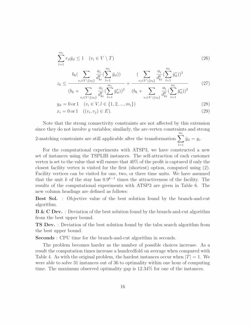
For the computational experiments with ATSP3, we have constructed a newset of instances using the TSPLIB instances. The self-attraction of each customervertex is set to the value that will ensure that 40% of the profit is captured if only theclosest facility vertex is visited for the first (shortest) option, computed using (2).Facility vertices can be visited for one, two, or three time units. We have assumedthat the unit k of the stay has 0.9k−1 times the attractiveness of the facility. Theresults of the computational experiments with ATSP3 are given in Table 6. Thenew column headings are defined as follows:

Best Sol. : Objective value of the best solution found by the branch-and-cutalgorithm.

B & C Dev. : Deviation of the best solution found by the branch-and-cut algorithmfrom the best upper bound.

TS Dev. : Deviation of the best solution found by the tabu search algorithm fromthe best upper bound.

Seconds : CPU time for the branch-and-cut algorithm in seconds.

The problem becomes harder as the number of possible choices increase. As aresult the computation times increase a hundredfold on average when compared withTable 4. As with the original problem, the hardest instances occur when |T | = 1. Wewere able to solve 31 instances out of 36 to optimality within one hour of computingtime. The maximum observed optimality gap is 12.34% for one of the instances.

16

We have adapted the tabu search algorithm described in Section 5 to cope withthe extended problem, by simply adding a copy of each vertex to the graph for eachextra unit of stay, with the associated attraction value modified appropriately. Wewould like to comment here that this approach is not feasible for the case whenextra units of stay are actually more attractive than the first ones, i.e., the marginalgain is increasing. However, this case is not likely to be observed in practice. Thedeviations of the results of the tabu search algorithm are also included in Table 6.The average deviation is 1.92%, whereas the maximum run time is about a minute.

8 Conclusion

We have defined, analyzed, and solved a variant of the TSP, where the profit isattracted from customer vertices by visiting facility vertices, rather than collectedby visiting customer vertices. We have used a non-linear gravity demand allocationfunction to formulate the problem. A linearization scheme was devised using thelinear tangents of the concave portions of the objective function as valid inequalities,and a branch-and-cut algorithm, as well as a tabu search heuristic were implemented.We have also analyzed an extension of the original problem where more than oneservice option is allowed. The solution methods we have developed for the originalproblem can be adapted to the extended version in a straightforward manner. Wehave conducted computational experiments on randomly generated instances andon instances derived from TSPLIB. The solution values of our algorithms do notdeviate on the average by more than a few percents from the best upper boundvalue.

Acknowledgments: This work was partially funded by the Canadian Natural Sci-ences and Engineering Research Council under grants 227837-04 and 39682-05. Thissupport is gratefully acknowledged. The authors thank Stefan Ropke for providingthe code for an implementation of the Edmonds-Karp algorithm for the MaximumFlow Problem.

17

Bibliography

[1] D.R. Bell, T.-H. Ho, and C.S. Tang, Determining Where To Shop: Fixed andVariable Costs of Shopping, Journal of Marketing Research 35 (1998), 352-370.

[2] H.P. Benson, On the Global Optimization of Sums of Linear Fractional Func-tions over a Convex Set, Journal of Optimization Theory and Applications 121(2004), 19-39.

[3] T. Drezner, Competitive Facility Location in the Plane, Facility Location: ASurvey of Applications and Methods, Z. Drezner (Editor), Springer, Berlin(1995), pp 285-300.

[4] T. Drezner and Z. Drezner, A Note on Applying the Gravity Rule to theAirline Hub Problem, Journal of Regional Science 41 (2001), 67-73.

[5] T. Drezner and Z. Drezner, Validating the Gravity-Based Competitive Loca-tion Model Using Inferred Attractiveness, Annals of Operations Research 111(2002), 227-237.

[6] T. Drezner and Z. Drezner, Finding the Optimal Solution to the Huff BasedCompetitive Location Model, Computational Management Science 1 (2004),193–208.

[7] T. Drezner and Z. Drezner, Multiple Facilities Location in the Plane Usingthe Gravity Model, Geographical Analysis 38 (2006), 391-406.

[8] T. Drezner and Z. Drezner, The Gravity p-Median Model, European Journalof Operational Research 179 (2007), 1239-1251.

[9] J. Edmonds and R.M. Karp, Theoretical Improvements in Algorithmic Effi-ciency for Network Flow Problems, Journal of the Association for ComputingMachinery 19 (1972), 248–264.

[10] H.A. Eiselt and G. Laporte, Demand Allocation Functions, Location Science6 (1998), 175–187.

[11] D. Feillet, P. Dejax, M. Gendreau, Traveling Salesman Problems With Profits,Transportation Science 39 (2005), 188–205.

18

[12] M. Fischetti, J. J. Salazar Gonzalez, and P. Toth, Solving the OrienteeringProblem through Branch-And-Cut. INFORMS Journal on Computing 10(1998), 133-148.

[13] R.W. Freund and F. Jarre, Solving the Sum-of-Ratios Problem by an Interior-Point Method, Journal of Global Optimization 19 (2001), 83–102.

[14] J.M. Gauthier and G. Ribiere, Experiments in Mixed-Integer Linear Program-ming Using Pseudo-Costs, Mathematical Programming 12 (1977), 26-47.

[15] M. Gendreau, G. Laporte, and F. Semet, The Covering Tour Problem, Oper-ations Research 45 (1997), 568-576.

[16] M. Gendreau, G. Laporte, and F. Semet, A Tabu Search Heuristic for theUndirected Selective Traveling Salesman Problem, European Journal of Oper-ational Research 106 (1998), 539-545.

[17] M. Gendreau, A. Hertz, and G. Laporte, New Insertion and Postoptimiza-tion Procedures for the Traveling Salesman Problem, Operations Research 40(1992), 1086–1094.

[18] B.L. Golden, L. Levy, and R. Vohra, The Orienteering Problem, Naval Re-search Logistics 34 (1987), 307–318.

[19] M.J. Hodgson, G. Laporte, and F. Semet, A Covering Tour Model for PlanningMobile Health Care Facilities in Suhum District, Ghana, Journal of RegionalScience 38 (1998), 621–638.

[20] D.L. Huff, Defining and Estimating A Trade Area, Journal of Marketing 28(1964), 34-38.

[21] D.L. Huff, A Programmed Solution for Approximating an Optimum RetailLocation, Land Economics 42 (1966) 293-303.

[22] A.K. Jain and V. Mahajan, Evaluating the Competitive Environment in Re-tailing Using Multiplicative Competitive Interactive Models, Research in Mar-keting 2, J. Sheth (Editor), JAI Press, Greenwich, 1979, pp. 217–235.

[23] S. Kataoka and S. Morito, An Algorithm for the Single Constraint Maxi-mum Collection Problem, Journal of Operations Research Society of Japan 31(1988), 515-530.

19

[24] M. Labbe, G. Laporte, I. Rodriguez-Martın, and J. J. Salazar Gonzalez, TheRing Star Problem: Polyhedral Analysis and Exact Algorithm, Networks 43(2004), 177–189.

[25] M. Labbe, G. Laporte, I. Rodriguez-Martın, and J. J. Salazar Gonzalez, Lo-cating median cycles in networks, European Journal of Operational Research160 (2005), 457–470.

[26] G. Laporte and S. Martello, The Selective Traveling Salesman Problem, Dis-crete Applied Mathematics 26 (1990), 193-207.

[27] Y. Lee, S.Y. Chiu, and J. Sanchez, A Branch and Cut Algorithm for theSteiner Ring Star Problem, International Journal of Management Science 4(1998), 21-34.

[28] J.R. Oppong and M. J. Hodgson, Spatial Accessibility to Health Care Facilitiesin Suhum District, Ghana, The Professional Geographer 46 (1994), 199–209.

[29] M.W. Padberg and G. Rinaldi, Facet Identification for the Symmetric Travel-ing Salesman Polytope, Mathematical Programming 47 (1990), 219–257.

[30] W.J. Reilly, The Law of Retail Gravitation, Knickerbocker Press, New York,1931.

[31] G. Reinelt, TSPLIB - A Traveling Salesman Problem Library, ORSA Journalon Computing 3 (1991), 376–384.

[32] S. Schaible, Fractional Programming, Handbook of Global Optimization, R.Horst and P. M. Pardalos (Editors), Kluwer, Dordrecht, 1995, pp. 495–608.

[33] S. Schaible, Fractional Programming with Sums of Ratios, Scalar and VectorOptimization in Economic and Financial Problems, E. Castagnoli, and G.Giorgi (Editors), Elioprint, Milano, 1996, pp. 163–175.

20

Figure 1: The graph of f(wk) = wk

bk+wk

21

|T | |W | Succ. Avg.Dev.

Max.Dev.

Arc-vertex Str. Conn. Str. 2-Match Lin. Nodes Toursize

Seconds

1 50 5 0.00% 0.00% 119.20 0.00 86.20 479.80 384.00 23.00 42.411 100 5 0.00% 0.00% 115.40 0.00 81.80 1356.60 614.60 22.80 114.941 150 5 0.00% 0.00% 125.60 0.00 182.60 2936.00 1792.60 23.40 668.0712 50 5 0.00% 0.00% 52.40 182.80 36.00 294.40 260.60 31.60 7.4912 100 5 0.00% 0.00% 103.15 45.70 96.65 795.40 463.20 31.20 22.2612 150 5 0.00% 0.00% 81.40 380.60 226.80 1743.00 1619.00 30.60 193.1325 50 5 0.00% 0.00% 25.60 350.20 201.60 155.20 413.60 41.20 17.3925 100 5 0.00% 0.00% 31.20 353.00 170.80 422.20 251.80 41.80 12.9425 150 5 0.00% 0.00% 58.75 262.46 146.37 814.40 244.60 40.80 21.6337 50 5 0.00% 0.00% 13.40 414.40 332.20 147.20 248.80 44.80 14.1237 100 5 0.00% 0.00% 15.80 513.40 254.80 356.00 683.80 44.80 44.2737 150 5 0.00% 0.00% 28.95 378.69 221.15 522.40 52.60 45.20 5.68

Table 1: Average computational results for |V | = 50.

22

|T | |W | Succ. Avg.Dev.

Max.Dev.

Arc-vertex Str. Conn. Str. 2-Match Lin. Nodes Toursize

Seconds

1 75 4 0.07% 0.34% 291.40 0.00 456.20 1607.60 1596.20 22.20 1738.681 150 5 0.00% 0.00% 252.00 0.00 196.60 3399.60 2680.20 23.20 2293.771 225 1 0.60% 1.14% 282.80 0.00 203.60 5982.80 1397.00 23.40 3303.8718 75 5 0.00% 0.00% 115.80 947.00 377.80 738.20 755.00 35.60 193.3918 150 5 0.00% 0.00% 115.40 817.00 349.40 1913.20 1347.80 35.60 340.4518 225 5 0.00% 0.00% 118.40 623.40 168.20 2817.20 1598.20 35.40 490.7137 75 5 0.00% 0.00% 67.00 1105.60 590.80 577.60 2598.80 51.60 323.0737 150 5 0.00% 0.00% 68.60 1055.60 396.40 1076.80 1142.40 51.00 112.3437 225 5 0.00% 0.00% 77.00 1389.00 718.00 1747.80 1615.80 50.20 295.2156 75 5 0.00% 0.00% 10.60 341.60 223.00 166.40 26.20 69.00 4.7556 150 5 0.00% 0.00% 21.00 780.20 414.40 467.80 188.40 68.40 26.5356 225 5 0.00% 0.00% 22.40 986.80 558.60 844.60 460.00 66.20 60.07

Table 2: Average computational results for |V | = 75.

23

|T | |W | Succ. Avg.Dev.

Max.Dev.

Arc-vertex Str. Conn. Str. 2-Match Lin. Nodes Toursize

Seconds

1 100 1 0.69% 2.47% 402.60 0.00 304.20 2077.80 775.60 26.60 3382.101 200 0 1.28% 2.02% 360.00 0.00 120.60 4607.60 537.80 28.00 3602.681 300 0 2.09% 4.11% 367.40 0.00 101.40 6741.20 236.20 25.20 3602.0125 100 4 0.02% 0.06% 138.40 1348.80 461.60 1375.40 1128.80 40.40 875.2525 200 3 0.22% 0.87% 199.40 2448.00 645.40 2959.80 1117.60 41.20 2582.5425 300 0 0.78% 1.13% 189.60 2577.80 647.20 5424.40 1360.20 41.00 3601.4650 100 4 0.03% 0.09% 109.20 4104.80 873.80 917.40 2217.40 61.60 1135.7050 200 5 0.00% 0.00% 81.20 1560.00 456.40 1634.20 778.40 61.40 297.3250 300 5 0.00% 0.00% 85.00 2160.40 991.00 3166.40 3107.80 61.20 1279.3475 100 3 0.01% 0.02% 49.00 4928.80 2865.80 404.20 6408.40 82.80 1846.4175 200 5 0.00% 0.00% 40.20 2526.20 1401.40 832.80 2054.80 82.40 740.4475 300 5 0.00% 0.00% 35.80 1933.40 858.00 1260.60 810.60 82.00 228.47

Table 3: Average computational results for |V | = 100.

24

Data file |V | |T | |W | Opt. Toursize

Seconds Data file |V | |T | |W | Opt. Toursize

Seconds

kroA100.tsp 25 1 75 3208.87 11 34.06 kroB150.tsp 37 18 113 4775.70 23 2.12kroA100.tsp 25 6 75 3415.33 15 8.16 kroB150.tsp 37 27 113 4907.78 30 0.99kroA100.tsp 25 12 75 3491.10 19 1.72 kroB200.tsp 50 1 150 5158.18 13 147.86kroA100.tsp 25 18 75 3562.48 24 0.06 kroB200.tsp 50 12 150 5122.27 19 627.50kroA150.tsp 37 1 113 4781.18 12 381.00 kroB200.tsp 50 25 150 5725.12 30 10.31kroA150.tsp 37 9 113 5083.13 17 106.79 kroB200.tsp 50 37 150 6001.81 39 2.25kroA150.tsp 37 18 113 5319.77 24 25.27 kroC100.tsp 25 1 75 2910.12 11 10.48kroA150.tsp 37 27 113 5417.65 31 1.42 kroC100.tsp 25 6 75 3055.04 15 2.86kroA200.tsp 50 1 150 5571.03 13 2047.76 kroC100.tsp 25 12 75 3119.39 17 2.84kroA200.tsp 50 12 150 5777.59 18 83.27 kroC100.tsp 25 18 75 3237.36 22 0.32kroA200.tsp 50 25 150 6334.22 28 11.13 kroD100.tsp 25 1 75 3002.30 13 8.15kroA200.tsp 50 37 150 6584.07 38 3.75 kroD100.tsp 25 6 75 3094.04 16 0.89kroB100.tsp 25 1 75 3074.84 12 1.35 kroD100.tsp 25 12 75 3146.34 19 0.14kroB100.tsp 25 6 75 3046.43 14 5.08 kroD100.tsp 25 18 75 3170.25 23 0.04kroB100.tsp 25 12 75 3149.02 19 0.32 kroE100.tsp 25 1 75 3311.27 12 3.77kroB100.tsp 25 18 75 3194.25 23 1.15 kroE100.tsp 25 6 75 3313.15 14 0.91kroB150.tsp 37 1 113 4278.50 12 513.81 kroE100.tsp 25 12 75 3393.93 19 2.18kroB150.tsp 37 9 113 4553.95 17 42.83 kroE100.tsp 25 18 75 3474.43 24 0.11

Table 4: Computational results for the instances adapted from TSPLIB.

25

|V | |T | |W | Succ. Avg. Dev. Max. Dev. Tour size Seconds50 1 50 2 0.09% 0.23% 22.60 6.0850 1 100 3 0.08% 0.24% 22.40 8.4350 1 150 2 0.11% 0.36% 22.20 11.8550 12 50 2 0.03% 0.09% 31.20 9.5650 12 100 0 0.08% 0.25% 30.80 10.9450 12 150 1 0.10% 0.18% 30.20 10.8950 25 50 3 0.03% 0.07% 41.20 6.7350 25 100 2 0.06% 0.11% 41.60 8.1350 25 150 3 0.06% 0.16% 40.80 10.7750 37 50 4 0.01% 0.02% 44.60 4.3650 37 100 3 0.06% 0.20% 44.60 6.3550 37 150 4 0.01% 0.03% 45.20 5.3275 1 75 3 0.14% 0.51% 21.80 15.2175 1 150 2 0.24% 0.41% 22.40 22.5175 1 225 0 1.09% 1.98% 21.80 25.0575 18 75 0 0.08% 0.19% 35.20 23.3875 18 150 3 0.07% 0.18% 35.20 30.0775 18 225 2 0.12% 0.37% 35.20 30.9175 37 75 1 0.06% 0.08% 51.60 28.5275 37 150 3 0.06% 0.24% 51.00 26.9875 37 225 1 0.06% 0.18% 50.20 30.8175 56 75 2 0.07% 0.20% 68.60 13.3875 56 150 2 0.03% 0.05% 68.20 15.7975 56 225 0 0.11% 0.17% 65.80 14.82100 1 100 0 0.73% 1.96% 25.60 27.97100 1 200 0 1.66% 2.66% 25.40 29.42100 1 300 0 2.16% 3.25% 23.80 60.86100 25 100 0 0.26% 0.37% 40.00 41.98100 25 200 0 0.39% 1.14% 40.60 57.40100 25 300 0 0.95% 1.44% 40.20 93.39100 50 100 0 0.27% 0.53% 61.00 73.59100 50 200 0 0.19% 0.34% 61.00 88.28100 50 300 0 0.17% 0.40% 61.00 100.93100 75 100 0 0.14% 0.40% 82.60 36.21100 75 200 1 0.16% 0.43% 82.20 60.87100 75 300 0 0.12% 0.20% 82.00 62.63

Table 5: Average computational results for the tabu search heuristic.

26

Data file |V | |T | |W | Best Sol. B&C Dev. TS Dev. Tour size SecondskroA100.tsp 25 1 75 2356.94 3.38% 4.84% 9 3600.07kroA100.tsp 25 6 75 2588.61 0.00% 0.45% 10 550.52kroA100.tsp 25 12 75 2725.50 0.00% 0.06% 16 264.75kroA100.tsp 25 18 75 2879.12 0.00% 0.04% 20 385.60kroA150.tsp 37 1 113 3507.38 6.79% 7.24% 7 3600.16kroA150.tsp 37 9 113 3882.47 0.00% 0.74% 14 418.71kroA150.tsp 37 18 113 4166.33 0.00% 0.00% 20 37.11kroA150.tsp 37 27 113 4268.37 0.00% 0.00% 30 100.44kroA200.tsp 50 1 150 3695.43 12.34% 13.73% 10 3600.49kroA200.tsp 50 12 150 3938.35 0.00% 0.71% 17 1508.07kroA200.tsp 50 25 150 4545.33 0.00% 0.00% 28 748.35kroA200.tsp 50 37 150 4914.69 0.00% 1.32% 38 4.50kroB100.tsp 25 1 75 2574.24 0.00% 5.13% 7 5.26kroB100.tsp 25 6 75 2392.91 0.00% 0.00% 11 17.62kroB100.tsp 25 12 75 2507.46 0.00% 0.00% 15 19.84kroB100.tsp 25 18 75 2599.71 0.00% 0.00% 20 209.94kroB150.tsp 37 1 113 3041.24 7.64% 10.47% 8 3600.16kroB150.tsp 37 9 113 3282.68 0.00% 0.31% 15 320.64kroB150.tsp 37 18 113 3525.57 0.00% 0.00% 22 88.78kroB150.tsp 37 27 113 3700.55 0.00% 0.00% 29 8.97kroB200.tsp 50 1 150 3589.77 5.31% 7.28% 10 3600.30kroB200.tsp 50 12 150 3537.65 0.00% 0.27% 20 1984.54kroB200.tsp 50 25 150 4209.82 0.00% 0.01% 30 1700.38kroB200.tsp 50 37 150 4597.72 0.00% 0.00% 38 26.76kroC100.tsp 25 1 75 2114.73 0.00% 3.56% 8 1341.87kroC100.tsp 25 6 75 2287.62 0.00% 2.32% 10 310.89kroC100.tsp 25 12 75 2303.60 0.00% 0.00% 15 43.10kroC100.tsp 25 18 75 2524.49 0.00% 1.31% 18 0.87kroD100.tsp 25 1 75 2335.89 0.00% 1.25% 8 788.75kroD100.tsp 25 6 75 2435.53 0.00% 0.55% 12 190.42kroD100.tsp 25 12 75 2522.17 0.00% 1.10% 15 1.24kroD100.tsp 25 18 75 2642.82 0.00% 0.00% 19 6.66kroE100.tsp 25 1 75 2618.69 0.00% 3.53% 7 90.49kroE100.tsp 25 6 75 2561.26 0.00% 2.70% 10 9.03kroE100.tsp 25 12 75 2659.52 0.00% 0.31% 16 2.85kroE100.tsp 25 18 75 2766.34 0.00% 0.00% 22 46.59

Table 6: Computational results for the extended problem.

27