1

The Asset Pricing Implications of

Government Economic Policy Uncertainty*

Jonathan Brogaard

Andrew Detzel

November 2012

Abstract: Using a search-based measure to capture economic policy uncertainty for 21 countries, we find that when economic policy uncertainty increases by 1%, contemporaneous market returns fall by 2.9% and market volatility increases by 18%. An economic policy uncertainty factor-mimicking portfolio earns positive abnormal returns of 70 basis points per month and market-wide equity risk premiums increase for at least two years. Aggregate cash flows, especially private investment experience a level shift downward but return to normal growth rates after one quarter. Our results suggest that indecisiveness in government economic policymaking has material and long-lasting real and financial implications. * We have benefited from discussions with Scott Baker, Nicholas Bloom, Zhi Da, Alan Hess, Lubos Pastor, Stephan Siegel, and Mitchell Warachka. We also appreciate helpful feedback from seminar participants at the University of Washington. All errors are our own. Contact: Jonathan Brogaard, Foster School of Business, University of Washington, (Email) brogaard@uw.edu, (Tel) 206-685-7822; Andrew Detzel, Foster School of Business, University of Washington, (Email) adetzel@uw.edu, (Tel) 206-543-0721.

2

I. Introduction

Mathematics professor John Allen Paulos famously quipped, “Uncertainty is the only

certainty there is.”1 Uncertainty about the future has real implications on economic agents’

behavior (Bernanke, 1983; Bloom, 2009; Bloom, Bond, and Van Reenen, 2007; Dixit, 1989).

Government policymakers can add another layer of uncertainty regarding fiscal, regulatory, or

monetary policy, which we refer to as economic policy uncertainty. Government economic

policy is important; in 2009 federal, state and local government expenditures in the United

States totaled $5.9 trillion, 42.45% of the gross domestic product.2 The ubiquity of government

policy makes it very hard to diversify against. Thus, uncertainty related specifically to the

economic policy of governments may impact financial markets.3 In this paper we test the asset

pricing implications of economic policy uncertainty.

To motivate what we mean by economic policy uncertainty, consider the political events

surrounding the U.S. debt ceiling debate during the summer of 2011. After months of debate,

congress passed a bill increasing the debt ceiling. However, after the bill passed on August 2,

2011, economic policy uncertainty had not been resolved. As part of the debt ceiling agreement,

the Joint Select Committee on Deficit Reduction was created to agree upon $1.5 trillion in

budget cuts over the next ten years by November 23, 2011. Economic policy uncertainty came

from both the uncertainty about whether an agreement would be made regarding the debt

ceiling, and the fact that many policy decisions were left unresolved in the bill that finally

passed.

1 A Mathematician Plays the Stock Market, by John Allen Paulos, Basic Books, 2003. 2 This is true even after deducting transfers from the federal to state governments. http://www.gpo.gov and http://www.census.gov. 3 Knight (1921) established a distinction between risk and uncertainty. Risk refers to the possibility of a future outcome for which the probabilities of the different possible states of the world are known. Uncertainty refers to a future outcome that has unknown probabilities associated with the different possible states of the world. When referring to economic policy uncertainty we mean uncertainty or risk as we do not take a stand on whether the probabilities of the future direction policymakers will take can be ascertained with any degree of certainty.

3

The above example is one instance of economic policy uncertainty. Such occurrences

frequently arise (e.g. tax changes, health care reform, and social security reform, to name a few

that have been discussed recently in the United States).4 Governments have large direct and

indirect influences on the environment in which the private sector operates (McGrattan, Ellen,

and Prescott, 2005). The debt ceiling debate exemplifies two important factors of the

importance of economic policy uncertainty: the passage of a law or rule alone does not mean the

uncertainty is resolved, and the values in question are of large economic significance.

In this paper we test the impact of economic policy uncertainty on asset prices. We

create an index similar to that of Baker, Bloom and Davis (2012) using the Access World News

database.5 We measure country-specific news for 21 countries at a monthly frequency to obtain

a large time-series and cross-sectional database of country economic policy uncertainty. In the

debt-ceiling example, our measure allows us to observe in an objective fashion the amount of

uncertainty leading up to, and following, the legislation’s passage. We show that economic

policy uncertainty increases the equity risk premium and decreases cash flows. The cash flow

impact lasts one quarter into the future, while the risk premium is heightened for over two

years.

The appeal of our measure is that it allows for a continuous tracking of policy risk

compared with the alternatives. Traditionally, empiricists have taken two approaches to

measuring the impact of policy on asset prices. Under the first approach, researchers conduct

event studies with respect to the date of the policy implementation.6 Although event studies

have the advantage of being well-documented with a timeline of events leading up to the

culmination of the event of interest, they can be artificially precise. As the example of the debt

4 There is interesting literature on policy reform including Brender and Drazen (2008), Drazen and Easterly (2001), and Fernandez and Rodrik (1991), 5 Measures based on news have become a useful way to observe certain behavior at a higher frequency than was allowed previously (e.g. Da, Engelberg, and Gao, 2010). 6 Some such papers include Ait-Sahalia, Andritzky, Jobst, Nowak, and Tamirisa (2010), Cutler (1988), Rigobon and Sack (2004), Sialm (2009), Thorbecke (1997), and Ulrich (2011).

4

ceiling debate makes clear, the passing of a bill does not necessarily indicate the resolution of all

uncertainty.

Under the second approach, studies use elections as a resolution of government

uncertainty (Belo, Gala, and Li, 2012; Boutchkova, Hitesh, Durnev, and Molchanov, 2012;

Durnev, 2010; Li and Born, 2006; Pantzalis, Stangeland, and Turtle, 2000; Santa-Clara and

Valkanov, 2003). Compared to a political election measure of economic policy uncertainty

resolution, the search news measure we employ has several advantages. First, news-based

economic policy uncertainty measures are available on an ongoing basis. Elections occur

infrequently and so only capture short intervals of uncertainty resolution. At the same time, as

relevant economic policy decisions change over time, it is problematic to use an election in the

current period as a measure of uncertainty resolution for forthcoming policy issues.

Second, news-based measures quantify uncertainty resolution rather than assume a new

regime resolves uncertainty. Although politicians provide statements about how they want to

set economic policy, there is no strong mechanism binding them to their statements. In

addition, economic policy is set in a dynamic political setting where compromises must be

made, legal and judicial hurdles must be incorporated, and many times more nuanced rule

making occurs by the appropriate administrative agency. For example, although President

Obama signed into law the Dodd-Frank Wall Street Reform and Consumer Protection Act on

July 21, 2010, the U.S Commodity Futures Trading Commission continues to write and clarify

rules relating to the bill. With a high-frequency sentiment measure, one can carry out precise

empirical tests that isolate the longer-term impact of economic policy uncertainty related to

specific decisions.

To capture country-specific economic policy uncertainty, we search the database of

Access World News, one of the largest news source aggregators. For each month between 1990

and 2012 we search for key terms such as “tax” and “regulation” jointly with words that convey

uncertainty such as “unsure” and “unclear.” Access World News returns all articles in its

5

database containing these key words. We capture the number of articles it returns and use the

frequency of articles about economic policy uncertainty to quantify the level of such uncertainty

in the economy. Because we are interested in cross-country variation, we also require the search

mentions the country’s name in order for the article to count towards a given country’s

economic policy uncertainty. There are more articles in more recent years, partly due to the

growth of news outlets, but more importantly due to the digitalization of virtually all modern-

news sources, and so we normalize the frequency of country-related economic policy uncertainty

by the total number of articles about that country in the selected month.

Our measure is a variation of the Baker, Bloom and Davis (2012) measure. We use a

similar keyword search as the Baker et al. (2012) paper. However, we extend it to an

international setting and utilize the extensive Access World News database. In addition, we

expand the possible keywords used to capture economic policy uncertainty. Finally, our measure

is a reduced form of the Baker et al. (2012) measure in that we focus solely on the news

component due to data availability issues of the other two components of their measure

(expiring tax regulations and forecaster variability) in the international setting.

We relate our economic policy uncertainty measure to market returns. Through a variety

of specifications in a simple OLS regression setting, we find a negative contemporaneous

correlation between changes in economic policy uncertainty and market returns, and a positive

relationship between current levels of economic policy uncertainty and future market returns.

Positive shocks to economic policy uncertainty coincide with a decline in prices, but higher

future returns. This is consistent with economic policy uncertainty having real asset pricing

implications, and leads one to think about the mechanism by which economic policy uncertainty

drives asset-pricing dynamics.

Next we tease out why increases in economic policy uncertainty result in lower

contemporaneous returns and why higher levels of economic policy uncertainty result in higher

future returns. From basic financial theory, a decrease in prices can be due to negative changes

6

in expected cash flows, or an increase in discount rates. Theoretical work shows that

uncertainty can impact future cash flows (Aizenman and Marion, 1993; Born and Pfeifer, 2011;

Hermes, and Lensink, 2001). Empirical work to date suggests there is an effect (Erb, Harvey,

and Viskanta, 1996; Hassett and Metcalf, 1999; Julio and Yook, 2012). The asset pricing effect of

economic policy uncertainty has not been thoroughly studied empirically, but there is a strong

theoretical foundation to it (Croce, Kung, Nguyen, and Schmid, 2011; Croce, Nguyen, and

Schmid, 2011; Gomes, Kotlikoff, and Viceira, 2011; Pastor and Veronesi, 2011 and 2012).

We find evidence that the effect comes from both changes to expected cash flows and

discount rates. When economic policy uncertainty increases, cash flows decrease, as seen

through a drop in gross domestic product (GDP). We consider which components of GDP

economic policy uncertainty affects by analyzing separately the three largest components:

investment, consumption, and government expenditure. We find that economic policy

uncertainty has a sizeable impact on private investment.

In addition, economic policy uncertainty commands a risk-premium in the cross-section

of U.S. stock returns. We sort U.S. stocks in the CRSP universe each month into equal-weighted

quintiles based on their estimate exposure to economic policy uncertainty. We find that the

portfolio that is long (short) in the quintile with the greatest (least) exposure to economic policy

uncertainty earns significant positive abnormal returns with respect to the standard Fama

French Three factor model and the Five factor model, augmented with the Carhart (1997)

momentum factor and the Pastor and Stambaugh (2003) liquidity factor.

Having shown that economic policy uncertainty impacts the discount rate as well as cash

flows, we extend the analysis to determine how long the impact lasts. If agents simply wait for

the policy uncertainty to be resolved before investing, we would see economic policy uncertainty

only temporarily impacting asset prices (McDonald and Siegel, 1986). Alternatively, economic

policy uncertainty may cause enduring changes in agents’ value-maximizing behavior.

7

To test the two different hypotheses, we repeat the analysis conducted earlier but

incorporate a lead-lag relationship between returns, cash flows, and economic policy

uncertainty. If the effect is temporary, we expect to see reversion in the coefficients – an initial

underperformance will subsequently be followed by over-performance. If the effect is

permanent, it could be so in two ways. First, it could be that the economic policy uncertainty

shifts asset prices down in a one-time event. We would see this in the results by cash flows

being below average for a few quarters and thereafter returning to normal. It would show up in

the discount rate by the cumulative expected returns increasing initially, but thereafter leveling

out. Alternatively, the effect could be permanent in that it could continue to decrease cash flows

and demand a higher discount rate beyond its initial impact. If this is the case, cash flows will

continue to underperform into the future and cumulative expected returns will remain elevated.

We test the alternative effects for up to two years into the future (eight quarters for the

GDP data and 24 months for the stock returns), and we find cash flows are permanently shifted

lower. Growth rates decrease for one quarter after an increase in economic policy uncertainty

and thereafter resume their normal growth rate. That is, the effect causes a permanent shift

downward; we do not observe above-average growth following the one quarter with below-

average results.

To examine the longevity of the risk premium implications, we follow Santa-Clara and

Valkanov (2003) and decompose returns into their expected and unexpected components. We

find that expected returns (risk premium) are permanently higher with an ongoing effect for at

least two years following an increase in economic policy uncertainty. The risk premium is

greater initially, and continues to be greater for the entire period of the analysis – the

cumulative expected returns are increasing with economic policy uncertainty even after two

years. These results hold after controlling for business cycle considerations. We find that a lack

of policy certainty has economically important and long-lasting implications for asset prices.

8

The paper is organized as follows. In Section II, we describe our data and the

construction of variables. Section III presents the results of our main specifications relating

economic policy uncertainty to stock returns. Section IV decomposes the effect on cash flows

and discount rates. Section V explores the longevity of asset pricing implications, and Section

VI concludes.

II. Data and variable construction

The data in this paper come from a variety of sources. We use the Datastream Total

Return Index as a measure of stock market performance in a given country. The total return

index represents the growth of a representative sample of stocks which cover over 75% of a

country’s total market capitalization, include dividends (and assumes they are reinvested), and

is value weighted by market capitalization. We also capture a country’s index dividend yield

from Datastream.

Quarterly Real GDP, private investment, private consumption, and government

consumption expenditure data come from IMF International Financial Statistics via

Datastream. We use the real GDP series I99B. As a proxy for private investment, we use the

real gross fixed capital formation series I93E. For real private consumption we use series I96F,

and for government expenditure we use series I91F. These variables are seasonally adjusted.

The inflation reference years differ from country to country, but our analyses always use first

differences of the logarithms of these variables, so the normalization is irrelevant.

We create a variety of business cycle variables from the International Monetary Fund

(IMF) series via Datastream that are used to capture the business cycle. BILL is the IMF short-

term treasury rate for each country if available (Datastream item I60C). For South Korea no

such treasury rate is available, and the Australian treasury bill series is discontinuous, so

9

following Hjalmarsson (2010), we use the central bank discount rate for these countries

(Datastream item I60). The IMF also has a long-term treasury series for countries (Datastream

item I61). TSP is the difference between this IMF long-term treasury yield and the country’s

BILL. Insufficient business cycle variable data were available for Brazil, China, Hong Kong,

India, the Netherlands and Russia, so they are excluded from analyses using the business cycle

variables.

Our objective is to build a measure that captures the degree of economic policy

uncertainty. We use an approach similar to Baker, Bloom and Davis (2012). They use three

distinct components to capture economic policy uncertainty: newspaper coverage, federal tax

code provisions set to expire, and disagreement between economic forecasters. Due to limited

availability of the tax code and economic forecaster disagreement for many countries, we focus

exclusively on a search-based newspaper coverage measure of economic policy uncertainty. We

use Access World News, a vast database of archived news stories from around the globe, to

create our measure. Access World News contains over 191 million articles from over 6,300 local,

regional, national, and international papers and news sources from around the globe. The

database covers from 1980 to today, with more recent years covering more media sources. We

perform all searches in English, as Access World News translates articles written in foreign

languages into English.

Each month, for a given country, we collect the frequency of articles describing a

country’s economic policy uncertainty and create the variable Economic Policy Uncertainty

(EPU). For an article to be an EPU article we require three criteria. First, an article must

mention the country of interest. For instance, when creating the index for Australia we require

that the word “Australia,” or one of its derivations, such as “Australia’s” or “Australian,” be

mentioned in the article. Second, to capture uncertainty, the article must contain at least one of

the following terms or its derivation: ambiguous, indecision, indefinite, indeterminate,

questionable, speculative, uncertain, unclear, unconfirmed, undecided, undetermined,

10

unresolved, unsure, vague, or variable. Finally, the article must discuss economic policy. In

particular, one of the following key terms must be used in an article to count as an article related

to economic policy uncertainty: budget, central bank, deficit, federal reserve, policy, regulation,

spend or tax. For each word, we also allow its various deviations, such as “regulate” or

“regulatory” to satisfy the policy discussion requirement.7

We mine the Access World News database for key terms in the text of the archives. We

restrict the possible news sources to magazines or newspapers. The level of news, and news

digitized, varies over time. To control for the increased volume of articles, we scale the raw

economic policy uncertainty article count by the number of articles that mention the country of

interest and contain the word “today.” We perform this search every month from January 1990

to March 2012. From this search we capture the total number of news articles in a given month

t for a specific country j. This value is used as a measure of how much overall news is being

produced and captured by Access World News. We scale the economic policy uncertainty

measure by the news intensity measure to create EPU. The final variable is multiplied by 100

and logged:

EPUj,t =Ln(100 * Number of Economic Policy Uncertainty Articlesj,t ). (1)

Total Number of Articlesj,t

In Table 1 we report summary statistics of the newly created measure. We use data from 21

countries: Australia, Brazil, China, Canada, England, France, Germany, Great Britain, Hong

Kong, India, Italy, Japan, Mexico, Malaysia, Netherlands, Russia, South Africa, South Korea,

Spain, Sweden, Switzerland and the United States. The 21 countries were chosen based on

having a stock market with a market capitalization of more than $500 billion at the beginning of

7 Our measure closely imitates Baker, Bloom and Davis (2012); see their paper for an in depth analysis of a similar search-based measure in the United States.

11

2011. Table 1 Column 2 reports the time period for which we have sufficient data to create EPU.

For most countries we have data from January 1990 through March 2012; however, Brazil,

China, and Russia have abbreviated time series (starting in 1994, 1993, and 1998, respectively).

Column 3 shows the average value of EPU for each country. It ranges between 2.333

(India) and 3.257 (Hong Kong). The standard deviation of EPU is reported in Column 4 and

ranges between 0.0057 (UK) and 0.0243 (Brazil). Besides the level of EPU, we are interested in

the change in EPU, ΔEPU. The level provides information about the degree of economic policy

uncertainty for country j in month t. The change offers evidence on the innovation in economic

policy uncertainty. Both are of interest: a shock to economic policy uncertainty is new

information for which there may be a price reaction; the level, on the other hand, is fully known

(after accounting for the new innovation), but may still have implications for cash flows and

discount rates. We report the one-period (one-month) change in EPU in Columns 7 and 8.

INSERT TABLE 1 ABOUT HERE

One concern with studying economic policy uncertainty is that we are simply capturing

general uncertainty. To test this hypothesis we capture general economic concern by calculating

the standard deviation of a country’s total return index daily returns. Arnold and Vrugt (2008),

Bansal and Yaron (2004), Bittlingmayer (1998), and Veronesi (1999) show that economic

uncertainty causes asset price volatility. Thus, we create a variable, Uncertainty, for each

country-month, which is the standard deviation of daily returns for country j, in month t, given

by the daily Datastream Total Return Index, and multiplied by 100. Column 5 reports each

country’s mean, and Column 6 its standard deviation; while Columns 9 and 10 do the same for

its first difference. The correlation between Uncertainty and EPU is only 0.1836 (and 0.0527

between their first differences), so we are capturing an effect distinct from that of general

uncertainty.

12

Restricting momentarily to the United States, we consider the logarithm of the U.S. VIX

index, a measure of economic uncertainty, and our EPU index. Figure 1 plots the time series of

the U.S. VIX index and our EPU index. Beber and Brandt (2009) and Ederington and Lee

(1996) suggest that measures of implied volatility on major market indices, such as VIX, capture

economic uncertainty because financial markets reflect macroeconomic fundamentals. The

correlation between the U.S. VIX and EPU is 0.1957. When VIX goes up, EPU generally does as

well. However, a large proportion of the VIX measure of general uncertainty moves

independently of EPU.8

INSERT FIGURE 1 ABOUT HERE

Table 2 shows the country-pairwise correlations between EPU. For most countries the

correlations are relatively low, with the median correlation 0.39. An extant literature shows

there is significant international correlation of economic variables (Ambler, Cardia, and

Zimmermann, 2004; Baxter and Crucini, 1993; Canova, 1998; Roll, 1988) and therefore some

joint movement is not unexpected, but there is wide variation with the variability, often

consistent with intuition. For instance, Germany and France have a correlation coefficient of

0.71, whereas the Netherlands and Australia have a -0.03 correlation coefficient. We exploit this

variation in the rest of the paper to produce a panel dataset to study the implications of

economic policy uncertainty on asset prices.

INSERT TABLE 2 ABOUT HERE

8 We reproduce Figure 1 with the Baker, Bloom, and Davis (2012) economic policy uncertainty index as well. The graph is qualitatively similar but the correlation is higher (0.5578) between the Baker et al. index and the VIX.

13

III. Economic Policy Uncertainty and Stock Returns

In this section we establish that economic policy uncertainty affects contemporaneous

and future stock market returns. Furthermore, we document that increases in policy

uncertainty result in an increase in asset price volatility.

a. Stock Returns

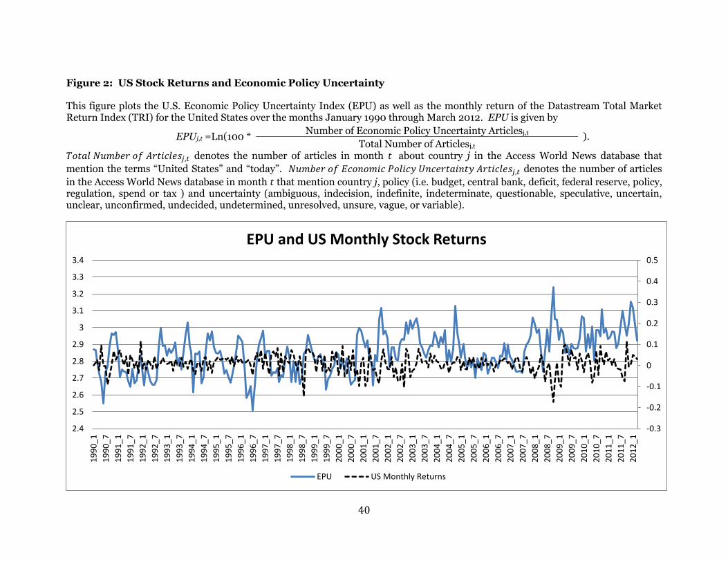
Figure 2 plots the U.S. economic policy uncertainty index with the U.S. monthly return

time series.

INSERT FIGURE 2 ABOUT HERE

The correlation between the two is -0.102. We formally measure this relationship in the

international setting.9

To measure the link between stock returns and economic policy uncertainty we estimate

a variety of panel regressions of the form:

(2)

where denotes the country and the month. The returns are one-month holding period

returns measured by the Datastream total market return index for country during month . For

clarity of timing, note that EPUt-1 is the level of EPU during the month t-1, calculated using news

between the beginning of month t-1 and the end of month t-1. Forward-looking expectations of

9 We reproduce Figure 2 with the Baker, Bloom, and Davis (2012) index. It is qualitatively similar although their index has a considerably lower, but still positive, correlation of 0.0435 with the US Total Return Index.

tjr ,

14

month t are based on EPUt-1. The vector used in different specifications of Equation 2

includes different combinations of levels and first differences of the natural logarithms of

Uncertainty and Economic Policy Uncertainty indices, and , respectively.

Under the null hypothesis where economic policy uncertainty has no effect on prices, the beta on

ΔEPUt and EPUt-1 should equal zero in the regression. Each regression includes country-fixed

effects ( to prevent unobserved heterogeneity across countries from biasing the

coefficients. Table 3 reports the results. The t-statistics are reported in parentheses below the

coefficients, and standard errors are double-clustered by country and month. Clustering

standard errors by month allows for arbitrary cross-sectional correlation, which is a possibility

given the potential regional and/or global nature of economic shocks. Clustering by country

allows for heteroskedasticity across countries.

INSERT TABLE 3 ABOUT HERE

Column 1 shows that in a simple univariate regression the contemporaneous relationship

between ΔEPUt and stock returns is significantly negative, with an increase in economic policy

uncertainty associated with a significant drop in prices. Similar results hold for the measure of

general uncertainty described in Section II, ΔUncertaintyt (Column 2). General uncertainty also

tends to increase while contemporaneous stock prices decline. Intuitively, a negative shock to

the macro economy, including one to economic policy uncertainty would tend to increase

volatility and decrease stock prices. When including both ΔEPUt and ΔUncertaintyt in Column

3, both are statistically significant.

The results in Column 3 suggest that general uncertainty and economic policy

uncertainty can be distinguished from each other. Also, the increase in the Adjusted R-squared

between Columns 1 and 2 (0.004 and 0.042, respectively), and Column 3 (0.046) suggests that

the two types of uncertainty explain different aspects of stock returns.

tjI ,

15

Column 4 focuses on the level effect of EPU. The regression specification includes both

the contemporaneous level, EPUt, as well as the one-month lagged level, EPUt-1. This is

necessary considering the level of EPUt is problematic: Column 1 shows that an increase in EPUt

results in a negative return. At the same time, though, we hypothesize that persistent high

economic policy uncertainty will produce a higher risk premium, and thus higher returns. The

two effects could be offsetting. To isolate the different effects we include the one-period lag and

the contemporaneous level of EPU. EPUt has a negative coefficient (-3.061) while EPUt-1 has a

positive one (2.810) and both are statistically significant. The coefficient signs are consistent

with the hypothesis that there is a risk premium associated with economic policy uncertainty,

and innovations in EPU affect stock prices. Column 5 does the same analysis on the general

uncertainty level variable. The results are similar – a positive coefficient on the lagged variable,

and a negative coefficient on the contemporaneous one. The sign and statistical significance is

robust to combining the two types of uncertainty (Column 6).

b. Volatility

To test the hypothesis that higher economic policy uncertainty results in lower

immediate returns and higher future returns via an increase in risk, we examine whether

volatility increases with economic policy uncertainty. Such a difference in riskiness would arise

from differences in economic policies being less clear in their economic impact or having more

hurdles to overcome before becoming definitive. If there were a difference in the riskiness of the

stock market following economic policy uncertainty, it could possibly command a positive risk

premium to compensate investors for the greater risks incurred in those periods. We investigate

this hypothesis by measuring the volatility of returns contemporaneous and following changes

in the level of economic policy uncertainty.

16

If increases in the EPU index are, ceteris paribus, associated with increases in a country’s

macroeconomic risk, then market return volatility should be higher the month following an

increase in the EPU. To test whether an increase in EPU is associated with an increase in

volatility, we first run a regression of the change in monthly volatility, ∆Volatility, calculated as

the first difference of the logged standard deviation of the within-month daily returns of month t

for country j on the change in economic policy uncertainty in month t for country j:

(3)

wherein the first specification , and in the remaining specifications, contains control

variables described below. If is positive, then increases in the ∆EPU are associated with

increases in monthly return volatilities, ∆Volatilityj,t. If is also positive it suggests the effect

persists. If and lose their significance with the inclusion of , then this relationship is due

only to ∆EPU acting as a proxy for business-cycle effects. Each regression includes country-

fixed effects ( . Table 4 reports the results. The t-statistics are reported in parentheses

below the coefficients and are computed using standard errors double-clustered by country and

month.

INSERT TABLE 4 ABOUT HERE

Column 1 shows the contemporaneous relationship, while Column 2 shows the one-

month lagged relationship. Interestingly, the lagged change in EPU has a larger impact than the

contemporaneous impact. The results from the univariate contemporaneous regression analysis

show that contemporaneous volatility increases by 7.67% when economic policy uncertainty

increases by 1%, but is not statistically significant. However, the one-period ahead volatility

increases by 18.8%, statistically significant at the 1% level. Still not controlling for other

17

variables, but now conditioning on both the contemporaneous and lagged ∆EPU, the excess

volatility increases by a statistically significant 18.2% and 26.3% with a 1% increase in

contemporaneous and lagged ∆EPU, respectively.

One explanation for the contemporaneous and one-month ahead correlation between

economic policy uncertainty and excess returns is based on a "proxy" effect. Changes in the

economic policy uncertainty might merely be proxying for variations in expected returns due to

business cycle fluctuations. Since variations in returns have been associated with business cycle

fluctuations (Campbell, 1991; Fama, 1991; and Campbell, Lo, and MacKinlay, 1997) and business

cycle fluctuations have been associated with political variables (Faust and Irons, 1999; Gonzalez,

2000; Alesina and Rosenthal, 1995; Alesina, Roubini, and Cohen, 1997; and Drazen, 2000), one

could hypothesize that the relationship between returns and a politically motivated variable

simply captures the reflection of the correlation between the business cycle and political

variables. If economic policy uncertainty were proxying for such business cycle factors, then the

observed relationship between economic policy uncertainty and returns would be unsurprising.

Hence, this relationship could disappear once we account for those factors.

To test the alternative hypothesis we include three variables that have been shown to be

associated with the business cycle and to forecast stock market returns: the log of dividend yield

DPt, the difference between the short-term and long-term interest rate TSPt, and the short-term

treasury rate Billt (Ang and Bekaert, 2007; Hjalmarsson, 2010). If the economic policy variable

contains only information about returns that can be explained by business cycle fluctuations,

then the coefficient of ∆EPU should equal zero. To avoid problems with seasonality of

dividends, we consider the 12-month moving average of dividend-yield although all results are

robust to non-seasonally adjusted dividend yields.

Columns 4 and 5 repeat the exercise performed in Columns 2 and 3, except they include

first differences of business cycle control variables. In the lagged-only analysis (Column 4), the

coefficient of ∆EPUt-1 remains statistically significant at 0.188. Conditioning on

18

contemporaneous and lagged values of ∆EPU (Column 5) also yields statistically significant

slopes that are qualitatively identical to their values without the controls (0.187 and 0.265

versus 0.182 and 0.263).

Overall, the volatility results indicate that macroeconomic risk, as measured by stock market

volatility, increases contemporaneously with, and following increases in, ∆EPU, even controlling

for other business cycle effects. This is consistent with a discount-rate explanation of the return

results in which a positive shock to economic policy uncertainty increases risk and therefore

expected excess returns. This manifests empirically in an immediate drop in prices followed by

higher average returns in the following months seen in Table 3.

IV. Decomposing the Effect on Cash Flows and Discount Rates

Section III shows that economic policy uncertainty has implications for asset returns.

Here, we begin to analyze the mechanism by which economic policy uncertainty influences asset

prices. We take as given the fact that contemporaneous stock returns decline and volatility

increases with increases in ∆EPU, while sustained higher levels of EPU are associated with

higher returns in the future. We now decompose the effect into a numerator (cash flow) or

denominator (discount rate) effect. Since positive shocks to ∆EPU are associated with decreases

in stock prices, and future returns are higher following periods of heighted EPU, economic

policy uncertainty must be associated with a cash-flow effect or a discount rate effect.

a. Cash Flows

If economic policy uncertainty has a cash-flow effect, then changes in GDP should be negatively

associated with changes in the EPU index. We consider aggregate GDP data as well as its

components, private investment as measured by gross fixed capital formation, private

consumption, and government expenditures. We exclude China in the cash flow analysis due to

19

lack of data. The data are available on a quarterly basis. As such, we calculate a quarterly ∆EPU

by taking the net sum of change in EPU over the corresponding three-month interval, for

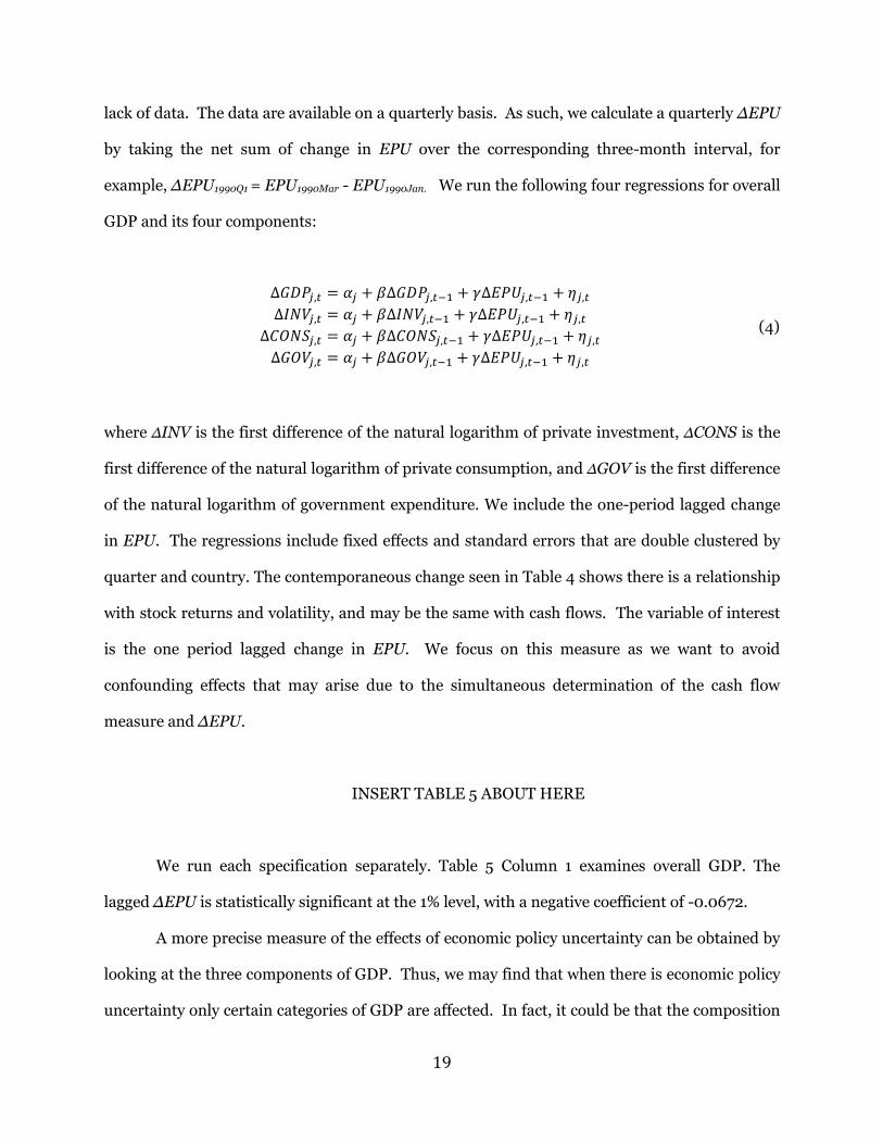
example, ∆EPU1990Q1 = EPU1990Mar - EPU1990Jan. We run the following four regressions for overall

GDP and its four components:

(4)

where ∆INV is the first difference of the natural logarithm of private investment, ∆CONS is the

first difference of the natural logarithm of private consumption, and ∆GOV is the first difference

of the natural logarithm of government expenditure. We include the one-period lagged change

in EPU. The regressions include fixed effects and standard errors that are double clustered by

quarter and country. The contemporaneous change seen in Table 4 shows there is a relationship

with stock returns and volatility, and may be the same with cash flows. The variable of interest

is the one period lagged change in EPU. We focus on this measure as we want to avoid

confounding effects that may arise due to the simultaneous determination of the cash flow

measure and ∆EPU.

INSERT TABLE 5 ABOUT HERE

We run each specification separately. Table 5 Column 1 examines overall GDP. The

lagged ∆EPU is statistically significant at the 1% level, with a negative coefficient of -0.0672.

A more precise measure of the effects of economic policy uncertainty can be obtained by

looking at the three components of GDP. Thus, we may find that when there is economic policy

uncertainty only certain categories of GDP are affected. In fact, it could be that the composition

20

of GDP changes. If we find that increases in lagged ∆EPU decreases investment and increases

consumption, that would also have meaningful implications for the effect of economic policy

uncertainty on economic performance.

Columns 2 – 4 consider the regression specification for each of the GDP components,

investment, consumption, and government expenditure, respectively. For investment and

consumption, lagged ∆EPU has a negative coefficient that is statistically significant at the 1%

level. When ∆EPU increases by 1% in period t, U.S. private investment in period t+1 decreases

by 0.125% on average. Consumption is also affected, with a coefficient of -0.033. While

government expenditures have a negative coefficient of -0.048, it is not statistically significant.

These results reject the null hypothesis that economic policy uncertainty has no effect on cash

flows. Indeed, at least part of the effect observed in the poor performance of asset prices

following increases in economic policy uncertainty is due to effects on the decline in private

investment.10

b. Discount Rates

Recent theoretical work suggests that economic policy uncertainty may demand a risk-

premium and be observable in the cross section of stock returns. Pastor and Veronesi (2012)

model firms with differing exposure to policy uncertainty. They posit that firms with higher

exposure to policy uncertainty typically have higher expected returns, although the phenomenon

is state-dependent and can potentially have the opposite effect.

To investigate the average cross-sectional effect of exposure to economic policy

uncertainty on expected returns, we focus exclusively on the cross-section of U.S. returns and

10 As an extra robustness check, we consider the first difference of the log market index as an additional right-hand-side variable in the GDP, Investment and Consumption regressions as markets are forward looking and incorporate all public information. The results from the Investment and GDP regressions are robust to its inclusions although the market change subsumes the significance in the Consumption regressions.

21

the U.S. EPU series. The data sample contains all U.S. CRSP stock returns between 1990 and

2011, the CRSP value-weighted market return, and the monthly U.S. Fama-French Three factors

and Momentum from Kenneth French’s website as well as the tradable Pastor Stambaugh

Liquidity factor from CRSP. We estimate ranking EPU betas, for each permno-month (i,m),

over the previous 60 months via the following regression:

( )

(5)

where and are the returns on stock and the three-month U.S. treasury bill for month ,

respectively.

We sort each stock into five equal-weighted portfolios for the ranking month.

These are the test assets. Note that when EPU increases, prices generally fall so that a more

negative EPU Beta indicates greater exposure to economic policy uncertainty. Stocks with the

highest economic policy uncertainty exposure will have the most negative EPU betas. Then, for

each portfolio we estimate the Fama French Three-Factor Model over the entire

sample period (starting in 1995, 60 months after sample begins):

( )

(6)

We repeat the analysis for the five factor model that also includes the Carhart (1997)

Momentum Factor (UMD), and the Pastor Stambaugh Liquidity Factor (LIQ), over the entire

sample period:

( )

(7)

22

We also construct a factor-mimicking portfolio (1-5) return by subtracting the first quintile

portfolio (most negative stocks) return from the fifth (least negative stocks) quintile

portfolio return and repeat the previous analysis. This generates a zero-investment portfolio

that is long in the first quintile portfolio and short in the fifth quintile portfolio.

Panel A presents average excess returns for each of the five portfolios sorted on and

the factor mimicking portfolio. Panel B presents the intercepts (abnormal returns or alpha) and

slopes of these five portfolios from the Fama French Three-Factor model. Panel C presents the

intercepts and slopes of these five portfolio returns using the Fama French Three-Factor model

augmented with the Carhart Momentum Factor and the Pastor Stambaugh Liquidity Factor.

Panel A reveals significant average returns that monotonically decrease from portfolio 1

(Column 1) to portfolio 5 (Column 5) consistent with earning positive returns for exposure to

EPU risk. On average, the high exposure quintile portfolio earns 63 basis points per month

more than the low quintile portfolio (Column 6).

Likewise, even controlling for the standard common risk factors, Panels B and C reveal

significant positive abnormal returns on the most EPU-risky portfolios and a monotonic decline

from the most EPU-risky portfolios to the least risky ones. In Panel B we see that the factor-

mimicking portfolio earns significant average abnormal returns of 59 basis points per month

with respect to the Fama French Three-Factor model. Including momentum and liquidity

slightly increases the estimated risk-adjusted returns of the factor-mimicking portfolio to a

monthly average of 70 basis points per month. We conclude that investors demand a risk

premium for holding stocks with a greater exposure to economic policy uncertainty captured by

our EPU measure. Figure 3 depicts the time series of the monthly returns obtained from

investing in the economic policy uncertainty factor-mimicking portfolio.

INSERT FIGURE 3 ABOUT HERE

23

V. Temporary or Permanent Effect

To understand the significance of the impact economic policy uncertainty has on asset prices we

analyze the longevity of the effects found in Sections III and IV.

a. Cash Flows

We again examine GDP as a national measure of cash flows, and also focus on its

components as in Table 5. Table 5 shows investment is particularly sensitive to economic policy

uncertainty, and consumption is moderately impacted. At the same time, government

expenditure is unaffected. In the following analysis we are interested in how long a shock to

economic policy uncertainty impacts GDP and private investment. To do so we rely on

autoregressive distributed lag models.

Autoregressive distributed lag models (ARDL’s) are time-series regressions of the form

(8)

Financial economists use ARDLs to identify relationships between a time-series and

another time-series that may depend on current and lagged values of each (e.g. Dailamia and

Hauswald, 2007; Dickson and Starleaf, 1974; Evans and Lyons, 2008; and Schwert, 1989).

Current and lagged variables’ effects can be important in financial and macroeconomic time-

series because economic decisions are made, and expectations are formed, using current and

past information. For example, financial market participants will consider both current and

prior changes in risk when determining their demand for risky assets. Then, macroeconomic

variables such as GDP may be relatively slow to fully react to contemporaneous events such as

24

increased economic policy uncertainty. A quarterly change in GDP could reflect

contemporaneous economic or policy events, as well as those in prior quarters. In general,

persistent effects not reflected in expectations also necessitate the inclusion of current and

lagged values of an explanatory variable.

To distinguish how long a change in EPU impacts cash flows, we extend the simple one-

lag model to one with two full years (eight quarters) of lagged ∆EPU. The regression

specification is:

∑ . (9)

All variables are as defined in previous tables. The results are in Table 7, Column 1.

INSERT TABLE 7 ABOUT HERE

Column 1 is the regression results of the specification in Equation 9. The t-statistics are

reported in parentheses below the coefficients, and standard errors are double-clustered by

country and month. The results show that, while the first lag of ∆EPU is still statistically

significant, the remaining coefficients are not (except for t-5). A shock to ∆EPU has an

economically meaningful impact on GDP for up to one quarter, but thereafter dissipates.

Thereafter, GDP resumes its normal growth path. It is also worth noting that there is no

subsequent statistically significant reversal in the signs of the coefficients over the next few

quarters, suggesting that the suppressed growth is not recovered by future above-average

growth. The fact that the coefficient no longer remains statistically significant after the first

quarter, and the longer-lagged variable coefficients diminish rapidly thereafter, suggests that

GDP growth experiences a level shift downward and resumes its normal level.

25

As Table 5, Column 2 shows, of the main components of GDP, EPU affects investment

the most. Thus, we repeat the above analysis for private investment:

∑ . (10)

∆EPU is significantly and negatively associated with changes in private investment again in the

initial quarter, but thereafter is no longer statistically significant. The results are in Table 7

Column 2. Like overall GDP, a shock to ∆EPU has an economically meaningful impact on

private investment growth for no more than one quarter. Also like the GDP results, the

coefficient does not reverse, suggesting a shift downward in investment as a result of the

economic policy uncertainty.

We repeat the analysis for private consumption, replacing in Equation 10

with . The first lag just misses statistical significance at the 10% level (t=-1.65), but has a

negative coefficient. When performing the ADL analysis on no discernible effect is

found. This is not surprising given the well-known persistence of consumption expenditures.

Tables 7 suggests that an increase in the U.S. EPU is associated with a meaningful,

though temporary, reduction in aggregate cash flows as measured by GDP. This reduction

comes primarily through a reduction in private investment. This is consistent with prior

literature (e.g. Julio and Yook, 2012) that shows firms reduce their investment as elections near,

as well as the theory of Pastor and Veronesi (2012) that suggests that “…firms should often cut

their investment in response to policy uncertainty.”

b. Returns

We ask a similar question on the longevity of the economic policy uncertainty impact on

returns. Unlike with the cash flow analysis, we need not include the prior lag variables as we

26

continue to look at the effect further out in time as market returns should rapidly (relative to

real production and investment) assimilate and respond to information contained in publicly

known information, such as innovations in economic policy uncertainty. The regression

specification is:

(11)

where is the market index holding period return of country from month t to month

for the values It is possible that the relationship between returns and the economic

policy uncertainty index comes from the index acting as a proxy for the phase of the business

cycle, or some other macro environment aspect not accounted for by dividend yield. We include

as control variables ( ) four business cycle variables: the log of dividend yield, DPt, the term

spread TSPt, the short-term treasury rate BILLt, the one-month lagged stock return volatility,

VOLt-1, and the U.S. default spread, SPREADt. We use Newey-West standard errors to account

for the serial correlation generated by using overlapping return windows, as well as

heteroskedasticity across countries. We also cluster standard errors at the month level.

INSERT TABLE 8 ABOUT HERE

If the economic policy uncertainty index is just a proxy for other macro risk, then these

macro economy control variables should load significantly, and and should equal 0.

Column 1 represents the coefficient for ∆EPUt, that is, the cumulative return associated with the

change in EPU. Column 2 is the standard error. Column 3 is the effect of the level of EPU on

future returns. Column 4 is its standard error. Finally, Column 5 is the Adjusted R-squared of

the regression in Equation 11. Each row extends the future horizon an additional month. Row 1

27

is the one-month return, Row 2 is the two-month holding period return, and this is repeated

until the 24-month cumulative return analysis is performed.

Column 1 shows that a 1% increase in ∆EPU is associated with a 2.685% decrease in the

contemporaneous month return, but as the holding period extends to two months (Row 2), the

effect becomes statistically insignificant.11 Thereafter, the coefficient remains statistically

insignificant for the rest of the test period (24 months). The decaying of the coefficient from

negative and statistically significant to statistically insignificant is consistent with the risk

premium analysis from Table 3: initially the shock accompanies a drop in prices, however the

higher EPU leads to higher risk-compensating expected returns going forward. The second

variable of interest in Table 8 is the level of EPU. For the level of EPU, the effect on future

returns is ambiguous. The coefficient is statistically insignificant, for all time intervals.

Theoretical work suggests that economic policy uncertainty should not only affect cash

flows, but may also impact discount rates. This would show up in the time-series of the risk

premia (in addition to the cross section, as seen in Section IV.b.) Pastor and Veronesi (2011)

provide a theoretical model in which economic policy uncertainty commands a risk premium.

In particular, their model predicts that the market will demand higher expected returns for

bearing the uncertainty about which policies policymakers will choose, what impact they will

have, and which political interests will win, precisely what our EPU measure aims to capture.

EPU increases when political factions compete. This uncertainty resolves only after a period of

political maneuvering, and the final policy choice is highly unpredictable ex ante. Furthermore,

the precise effects of various competing choices are largely unpredictable, as well as whether

they will survive legal objections brought through the judicial system.

In Section IV.b we showed there was a cross sectional effect associated with economic

policy uncertainty. To examine how long the risk-premia lasts after a shock to economic policy

11 We also form impulse response functions based on bivariate vector autoregressive models of excess returns and first difference log(EPU) with lag length chosen via the Bayesian Information Criterion, for each country. These show that shocks to EPU are assimilated into the country’s returns index within a quarter.

28

uncertainty, we focus on the time series risk premium commanded by economic policy

uncertainty. Unlike in Section IV.b we are able to carry out the analysis using the full

international dataset.

While the aggregate returns may not contain a lasting memory of EPU, the shock and

risk premia components may be offsetting each other. We proceed to investigate whether this

difference in realized returns can be attributed to an impact on the hypothesized time-series risk

premium charged by investors for economic policy uncertainty, or to unexpected returns. A

difference in expected returns would be consistent with economic policy uncertainty having an

impact on the risk premium. If the difference is due to unexpected returns being affected by

changes in economic policy uncertainty that would signal that the market is systematically

surprised by the lack of clarity in forthcoming economic policy.

To distinguish between the two hypotheses we rerun the analysis separating the changes

in expected and unexpected returns associated with changes in EPU. We decompose the

monthly returns for each country’s market index into expected and unexpected returns. The

expected returns are given by taking the fitted values from the regression of returns on the

lagged values of the predictability variables used in Equation 3: DPt, TSPt, Billt, VOLt-1, and

SPREADt. The unexpected returns are simply the residuals from this first regression. We

include both the lagged level as well as the contemporaneous change in economic policy

uncertainty as explanatory variables, ΔEPUt and EPUt-1. The economic hypothesis is as follows:

If ΔEPUt contains unexpected and relevant information, then we would expect that ΔEPUt

would not be a priced risk and therefore would not show up in the Expected Return analysis in

the initial time-windows. Over time, though, we expect the shock will be absorbed into the

premium demanded by investors. Thus we expect a positive coefficient in the longer time-

window periods. However, if an increase in economic policy uncertainty is a negative shock,

then the Unexpected Returns should decrease. Hence we expect that ΔEPUt will not be

statistically significant in the Expected Return regression at first, but later in the time window

29

will become positive. In the Unexpected Return regression we expect it to be negative initially

and eventually having no effect.

The hypothesis regarding the level of EPU is as follows. If EPU affects the price of risk

we expect to see it in the Expected Return regression. Specifically, we expect a positive

relationship between EPU and the price of risk, and hence predict higher returns following

heightened EPU and a positive coefficient. We have no theory on what the coefficient on the

level of EPU in the Unexpected Returns regression should be. If the other predictability

variables fully reflect the extent of return predictability, and the level of EPU adds no new

predictability, then the coefficient should be no different than zero. On the other hand, the

coefficient would be negative if it predicts low future unexpected returns, and positive if it

predicts high future unexpected returns.

We follow Santa-Clara and Valkanov (2003) and decompose monthly holding period

returns into expected and unexpected components to determine their relationships with ΔEPUt

and EPUt-1. For each country, j, and month, t, we consider the monthly holding period return.

To decompose the returns into their expected and unexpected components we follow a three-

step process. First, we regress the realized returns in period t on the predictors of market

returns – the controls in Equation 3: the beginning of the month dividend yield, DPt-1, the term

spread TSPt-1, the short-term treasury rate BILLt-1, the monthly stock market Volatility VOLt-1,

and the U.S. Default Spread, SPREADt-1:

(12)

Second, we use the estimated coefficients from Equation 12 to calculate the predicted, or

expected, return:

E( (13)

30

The residual is the surprise, or unexpected return:

( ) (14)

Finally, we regress the expected and unexpected returns on ∆EPU and EPU:

( ) (15)

(16)

In each regression step, we use heteroskedasticity-robust and month-clustered standard

errors. Table 9 Panel A presents estimates of Equation 15. Table 9 Panel B presents estimates of

Equation 16.

INSERT TABLE 9 ABOUT HERE

Table 9 Panel A reports the results for the expected return analysis, Panel B for the

unexpected returns. Panel A, Column 1, Row 1 indicates that a 1% increase in ∆EPU

corresponds to a positive although statistically insignificant effect on the contemporaneous

expected returns. However, after the first month (starting in Row 2) the effect becomes

statistically significant and positive at 67.4 basis points. The effect builds by around 30 to 50

basis points for most of the remaining months. This suggests that while the shock itself has only

a modest impact on expected returns, the effect it has on the level of EPU, does indeed become

an influential factor in determining the risk premium. Hence a positive shock to ∆EPU

31

corresponds to an economically large persistent increase in expected returns that lasts for

years.12

The positive relationship between economic policy uncertainty and expected returns is

further verified by the level variable, EPU. Column 3 focuses on the preexisting level of

economic policy uncertainty in time t-1. If the risk premium observed in Column 1 and in the

Fama Macbeth analysis in Table 6 is driven by the level of EPU, then we expect higher future

expected returns when current EPU is high. The first row shows a strong statistically significant

coefficient of 0.729. As the horizon of the cumulative return is stretched out further, the

coefficient almost uniformly increases by about 5o to 100 basis points, and the effect lasts for the

full two year horizon of study. Columns 2 through 24 show that the effect is persistent into the

future. This is true above and beyond the persistent effect a new shock to EPU has on expected

returns.

Pastor, Sinha and Swaminathan (2008) also find a positive relationship between

conditional market expected returns, as measured by implied cost of capital, and conditional

volatility of market returns. Similarly, we find international evidence that contemporaneous

increases in ∆EPU are associated with contemporaneous increases in volatility, and that higher

levels of EPU are associated with higher expected returns, consistent with a positive mean-

variance relationship between risk and return over time in market returns.

The estimates for unexpected returns in Panel B are drastically different from those

found in Table 9 Panel A. Column 1, Row 1 shows that a 1% increase in ∆EPU is associated with

a 2.807% drop in contemporaneous unexpected returns. Recall from Table 4 that an increase in

∆EPU is also associated with an increase in (conditional) volatility. Our results are consistent

with the Glosten et al. (1993) negative relationship between unexpected returns and conditional

volatility.

12 When investment decreases, the riskiest marginal projects likely will be eliminated first, hence EPU risk may “crowd out” non-EPU risk. Even so, we see increased risk premiums in spite of the fact that the adopted projects are less risky than they would be otherwise.

32

The shock to EPU is fully realized in the unexpected returns in a contemporaneous drop

in prices. A 1% higher level of one-period lagged EPU is associated with lower, but statistically

insignificant, unexpected returns. Policy uncertainty is rapidly priced into the market and only

the temporary price drop from a contemporaneous increase in economic policy uncertainty

manifests itself in unexpected returns. As the return window expands to two months, the effects

of the EPU shock are no longer noticeable in the unexpected component of returns.

VI. Conclusion

Government economic policy, including taxation, expenditure, monetary and regulatory

policy, has large, market-wide economic effects that are largely non-diversifiable. Economic

agents make real economic decisions based on expectations about the future economic policy

environment. Thus, even market-benevolent policymakers can increase risk by generating an

environment of uncertainty about their future economic policy decisions.

This paper extends the Baker, Bloom and Davis (2012) measure to an international

setting, creating a news-based index of economic policy uncertainty for a cross-section of

countries in order to determine the effects of economic policy uncertainty on asset prices. This

measure appears to be the first that quantifies the degree of economic policy uncertainty in an

asset pricing study. It is positively correlated, but distinct from general economic uncertainty.

Changes in economic policy uncertainty are in fact associated with significant cash flow and

discount-rate effects. Increases in economic policy uncertainty are negatively associated with

decreases in U.S. GDP for one quarter in the future. This is driven by a decrease in private

investment and consumption. The effect results in a one-time level downward shift with growth

presuming its regular rate thereafter.

The effect of economic policy uncertainty goes beyond a one-time shift in cash-flows. A 1%

increase in the economic policy uncertainty is associated with a contemporaneous 2.807%

33

decrease in the one-month unexpected return on the country-level market index. However, a 1%

increase in the level of economic policy uncertainty is associated with a 72.9 basis point increase

in expected one-month returns the following month, an effect that remains significant after two

years. This paper shows that economic policy uncertain has sizeable and enduring asset pricing

consequences.

34

References

Ait-Sahalia, Yacine, Jochen Andritzky, Andreas Jobst, Sylwia Nowak, and Natalia Tamirisa, 2010, Market Response to Policy Initiatives During the Global Financial Crisis, Working paper, NBER, No. 15809.

Aizenman, Joshua, and Nancy P. Marion, 1993, Policy Uncertainty, Persistence and Growth.

Review of International Economics Vol. 1, No. 2, 145-163. Alesina, Alberto, and Howard Rosenthal, 1995, Partisan Politics, Divided Government, and the

Economy (Cambridge University Press, Cambridge, UK.). Alesina, Alberto, Nouriel Roubini, and Gerald D. Cohen, 1997, Political Cycles and the

Macroeconomy (MIT Press, Cambridge, MA). Ambler, Steve, Emanuela Cardia, and Christina Zimmermann, 2004, International Business

Cycles: What are the Facts?, Journal of Monetary Economics, Vol. 51, 257-276. Arnold, I.J.M., and E.B. Vrugt, 2008, Fundamental Uncertainty and Stock Market Volatility,

Applied Financial Economics, Vol. 18, No. 17, 1425-1440. Ang, Andrew, and Geert Bekaert 2007, Stock Return Predictability: Is it There? Review of

Financial Studies, Vol. 20, No. 3, 651-707. Baker, Scott R., Nicholas Bloom, and Steven J. Davis, 2012, Measuring Economic Policy

Uncertainty, Working Paper. Bansal, Ravi, and Amir Yaron, 2004, Risks for the Long Run: A Potential Resolution of Asset

Pricing Puzzles, Journal of Finance, Vol. 59, No. 4, 1481-1509. Baxter, Marianne, and Mario J. Crucini, 1993, Explaining Saving – Investment Correlations, American Economic Review, Vol. 83, No. 3, 416-436. Belo, Frederico, Vito D. Gala, and Jun Li, 2012, Government Spending, Political Cycles, and the

Cross-Section of Stock Returns, Journal of Financial Economics, forthcoming. Bernanke, Ben S., 1983: Irreversibility, Uncertainty and Cyclical Investment, Quarterly Journal

of Economics, Vol. 98, 85–106. Bittlingmayer, George, 1998, Output, Stock Volatility, and Political Uncertainty in a Natural

Experiment: Germany, 1880-1940, Journal of Finance, Vol. 53, No. 6, 2243-2257. Bloom, Nicholas, 2009, The Impact of Uncertainty Shocks, Econometrica, Vol. 77, No. 3, 623-

685. Bloom, Nicholas, S. Bond, and J. Van Reenen, 2007, Uncertainty and Investment Dynamics,

Review of Economic Studies, Vol. 74 391–415. Born, Benjamin and Johannes Pfeifer, 2011, Policy Risk and the Business Cycle, Working paper.

35

Boutchkova, Maria, Doshi Hitesh, Art Durnev, and Alexander Molchanov, 2012, Precarious Politics and Return Volatility. Review of Financial Studies, Vol. 25, No. 4, 1111-1154.

Breen, William, Lawrence R. Glosten, and Ravi Jagannathan, 1989, Economic Significance of

Predictable Variations in Stock Index Returns, Journal of Finance, Vol. 44, 1177-1189. Brender, Adi, and Allan Drazen, 2008, How do Budget Deficits and Economic Growth affect

Reelection Prospects? Evidence from a large panel of countries, American Economic Review, 98, 2203–2220.

Campbell, John Y., 1987, Stock Returns and the Term Structure, Journal of Financial

Economics, Vol. 18, 373-399. Campbell, John Y., 1991, A Variance Decomposition for Stock Returns, Economic Journal 101,

157-179. Campbell, John Y., and Ludger Hentschel, 1992, No News is Good News: An Asymmetric Model

of Changing Volatility in Stock Returns, Journal of Financial Economics, Vol. 31, 281-318.

Campbell, John Y., Andrew Lo, and Craig MacKinlay, 1997, The Econometrics of Financial

Markets (Princeton University Press, Princeton, NJ). Canova, Fabio, 1998, Detrending and Business Cycle Facts, Journal of Monetary Economics,

Vol. 41, 475-512. Carhart, Mark M., 1997, On persistence in mutual fund performance, Journal of Finance, Vol. 52, 83–110.

Croce, Maximiliano M., Howard Kung, Thien T. Nguyen, and Lukas Schmid, 2011, Fiscal Policies and Asset Prices, Working Paper, University of North Carolina.

Croce, Maximiliano M., Thien T. Nguyen, and Lukas Schmid, 2011, The Market Price of Fiscal

Uncertainty, Working Paper, UNC. Cutler, David M., 1988, Tax Reform and the Stock Market: An Asset Price Approach, American

Economic Review, Vol. 78, 1107–1117. Da, Zhi, Joseph Engelberg, and Pengjie Gao, 2010, The Sum of all FEARS: Investor Sentiment

and Asset Prices, Working Paper. Dailamia, Mansoor, and Robert Hauswald, 2007, Credit-spread Determinants and Interlocking

Contracts: A Study of the Ras Gas project, Journal of Financial Economics, Vol. 86, 248–278.

Dickson, Harold, Dennis R. Starleaf, 1974, Polynomial Distributed Lag Structures in the Demand Function for Money, Journal of Finance, Vol. 27, No. 5, 1035-1043.

Dixit, Avinash, 1989, Entry and Exit Decisions Under Uncertainty, Journal of Political

Economy, Vol. 97, 620–638.

36

Drazen, Allan, 2000, Political Economy in Macroeconomics (Princeton University Press, Princeton, NJ).

Drazen, Allan, and William Easterly, 2001, Do Crises Induce Reform? Simple Empirical Tests of

Conventional Wisdom, Economics and Politics, Vol. 13, 129–157. Durnev, Art, 2010, The Real Effects of Political Uncertainty: Elections and Investment

Sensitivity to stock prices, Working Paper. Erb, Claude B., Campbell R. Harvey, and Tadas E. Viskanta, 1996, Political risk, Economic Risk,

and Financial Risk, Financial Analysts Journal, December, 29–46. Evans, Martin D.D., and Richard K. Lyons. 2008. How is Macro News Transmitted to Exchange

Rates? Journal of Financial Economics, Vol. 88, 26-50. Fama, Eugene F., 1991, Efficient Capital Markets: II, Journal of Finance, Vol. 46, 1575-1648. Fama, Eugene, and James MacBeth, 1973, Risk, Return, and Equilibrium: Empirical Tests,

Journal of Political Economy, Vol. 81, 607–636. Faust, Jon, and John S. Irons, 1999, Money, Politics and the Post-war Business Cycle, Journal of

Monetary Economics, Vol. 43, 61-89. Fernandez, Raquel, and Dani Rodrik, 1991, Resistance to Reform: Status Quo Bias in the

Presence of Individual-specific Uncertainty, American Economic Review, Vol. 81, 1146–1155.

French, Kenneth, G. William Schwert and Robert F Stambaugh, 1987, Expected Stock Returns

and Volatility, Journal of Financial Economics, Vol. 19, 3–29.

Glosten, Lawrence R., Ravi Jagannathan, and David E. Runkle 1993, On the Relation Between the Expected Value and the Volatility of the Nominal Excess Return on Stocks, Journal of Finance, Vol. 48, 1779-1801.

Gomes, Francisco J., Laurence J. Kotlikoff and Luis M. Viceira, 2011, The Excess Burden of

Government Indecision, Working paper. Gonzalez, Maria, 2000, Do Changes in Democracy affect the Political Budget Cycle? Evidence

from Mexico, Working paper, Princeton University. Hassett, Kevin A. and Gilbert E. Metcalf, 1999, Investment with Uncertain Tax Policy: Does

Random Tax Policy Discourage Investment?” Economic Journal, Vol. 109, No. 457, 372-393.

Hermes, Niels, and Robert Lensink, 2001, Capital Flight and the Uncertainty of Government

Policies, Economics Letters, Vol. 71, 377-381. Hjalmarsson, Erik, 2010, Predicting Global Stock Returns. Journal of Financial and

Quantitative Analysis, Vol. 45, No. 1, 49-80.

37

Julio, Brandon, and Youngsuk Yook, 2012, Political Uncertainty and Corporate Investment Cycles. Journal of Finance, Vol. 67, No. 1, 45-83.

Knight, Frank H. Risk, Uncertainty, and Profit, 1921, Library of Economics and Liberty. Li, Jinliang, and Jeffery A. Born, 2006, Presidential Election Uncertainty and Common Stock

Returns in the United States, Journal of Financial Research, Vol. 29, 609–622. McDonald, Robert, and Daniel Siegel, 1986, The Value of Waiting to Invest, Quarterly Journal

of Economics, Vol. 101, 707–728. McGrattan, Ellen R., and Edward C. Prescott, 2005, Taxes, Regulations, and the Value of U.S.

and U.K. Corporations, Review of Economic Studies, Vol. 72, 767–796. Nelson, Daniel B., 1991, Conditional Heteroskedasticity in Asset Returns: A New Approach,

Econometrica, 59, 347-370. Newey, W.K., and K.D. West, 1987, Hypothesis testing with efficient method of Moments

Estimation, International Economic Review, Vol. 28, No. 3, 777-787. Pagan, Adrian R., and Y. S. Hong, 1991, Nonparametric Estimation and the Risk Premium, in

William Barnett, James Powell, and George Tauchen, eds.: Nonparametricand Semiparametric Methods in Econometrics and Statistics, (Cambridge University Press, Cambridge), 51-75.

Pastor, Lubos, Robert Stambaugh, 2003, Liquidity Risk and Expected Stock Returns, Journal of

Political Economy, Vol. 111, No. 3. 642-685. Pastor, Lubos, Meenakshi Sinha and Bhaskaran Swaminathan, 2008, Estimating the

Intertemporal Risk-Return Tradeoff Using the Implied Cost of Capital, Journal of Finance, Vol. 63, No. 6. 2859-2897.

Pastor, Lubos, and Pietro Veronesi, 2011, Political Uncertainty and Risk Premia, Working

paper, University of Chicago. Pastor, Lubos, and Peitro Veronesi, 2012, Uncertainty About Government Policy and Stock

Prices. Journal of Finance (forthcoming). Pantzalis, Christos, David A. Stangeland, and Harry J. Turtle, 2000, Political Elections and the

Resolution of Uncertainty: The International Evidence, Journal of Banking and Finance, Vol. 24, 1575–1604.

Rigobon, Roberto, and Brian Sack, 2004, The Impact of Monetary Policy on Asset Prices,

Journal of Monetary Economics, Vol. 51, 1553-1575. Rodrik, Dani, 1991. Policy Uncertainty and Private Investment in Developing Countries, Journal

of Development Economics, Vol. 36, 229-242. Roll, Richard, 1988, The International Crash of October 1987, Financial Analysts Journal, Vol.

44, No. 5, 19-35.

38

Santa-Clara, Pedro, and Rossen Valkanov, 2003, The Presidential Puzzle: Political Cycles and the Stock Market. Journal of Finance, Vol. 58, No. 5. 1841-1872.

Schwert, G. William. 1989, Why does Stock Market Volatility Change over Time? Journal of

Finance, Vol. 44, No. 5, 1115-1153. Sialm, Clemens, 2009, Tax Changes and Asset Pricing, American Economic Review, Vol. 99,

1356–1383. Thorbecke, Willem, 1997, On Stock Market Returns and Monetary Policy, Journal of Finance

52, 635–654. Turner, Christopher M., Richard Startz, and Charles R. Nelson, 1989, A Markov Model of

Heteroskedasticity, Risk, and Learning in the Stock Market, Journal of Financial Economics, Vol. 25, 3-22.

Ulrich, Maxim, 2011, How Does the Bond Market Perceive Government Interventions? Working

Paper, Columbia University. Veronesi, Pietro, 1999, Stock Market Overreaction to Bad News in Good Times: A Rational

Expectations Equilibrium Model. Review of Financial Studies, Vol. 12, No. 5, 975-1007.

39

Figure 1: VIX and Economic Policy Uncertainty This figure plots the monthly U.S. Economic Policy Uncertainty Index (EPU) as well as the monthly-averaged Chicago Board Options Exchange S&P 500 Volatility Index (VIX) over the months January 1990 through March 2012. EPU is given by

EPUj,t =Ln(100 * Number of Economic Policy Uncertainty Articlesj,t

). Total Number of Articlesj,t

denotes the number of articles in month about country j in the Access World News database that

mention the terms “United States” and “today”. denotes the number of articles

in the Access World News database in month that mention country j, policy (i.e. budget, central bank, deficit, federal reserve, policy, regulation, spend or tax ) and uncertainty (ambiguous, indecision, indefinite, indeterminate, questionable, speculative, uncertain, unclear, unconfirmed, undecided, undetermined, unresolved, unsure, vague, or variable).

0

10

20

30

40

50

60

70

2.4

2.5

2.6

2.7

2.8

2.9

3

3.1

3.2

3.3

3.4

19

90

_1

19

90

_7

19

91

_1

19

91

_7

19

92

_1

19

92

_7

19

93

_1

19

93

_7

19

94

_1

19

94

_7

19

95

_1

19

95

_7

19

96

_1

19

96

_7

19

97

_1

19

97

_7

19

98

_1

19

98

_7

19

99

_1

19

99

_7

20

00

_1

20

00

_7

20

01

_1

20

01

_7

20

02

_1

20

02

_7

20

03

_1

20

03

_7

20

04

_1

20

04

_7

20

05

_1

20

05

_7

20

06

_1

20

06

_7

20

07

_1

20

07

_7

20

08

_1

20

08

_7

20

09

_1

20

09

_7

20

10

_1

20

10

_7

20

11

_1

20

11

_7

20

12

_1

EPU and VIX

EPU VIX

40

Figure 2: US Stock Returns and Economic Policy Uncertainty This figure plots the U.S. Economic Policy Uncertainty Index (EPU) as well as the monthly return of the Datastream Total Market Return Index (TRI) for the United States over the months January 1990 through March 2012. EPU is given by

EPUj,t =Ln(100 * Number of Economic Policy Uncertainty Articlesj,t ).

Total Number of Articlesj,t denotes the number of articles in month about country j in the Access World News database that

mention the terms “United States” and “today”. denotes the number of articles

in the Access World News database in month that mention country j, policy (i.e. budget, central bank, deficit, federal reserve, policy, regulation, spend or tax ) and uncertainty (ambiguous, indecision, indefinite, indeterminate, questionable, speculative, uncertain, unclear, unconfirmed, undecided, undetermined, unresolved, unsure, vague, or variable).

-0.3

-0.2

-0.1

0

0.1

0.2

0.3

0.4

0.5

2.4

2.5

2.6

2.7

2.8

2.9

3

3.1

3.2

3.3

3.4

19

90

_1

19

90

_7

19

91

_1

19

91

_7

19

92

_1

19

92

_7

19

93

_1

19

93

_7

19

94

_1

19

94

_7

19

95

_1

19

95

_7

19

96

_1

19

96

_7

19

97

_1

19

97

_7

19

98

_1

19

98

_7

19

99

_1

19

99

_7

20

00

_1

20

00

_7

20

01

_1

20

01

_7

20

02

_1

20

02

_7

20

03

_1

20

03

_7

20

04

_1

20

04

_7

20

05

_1

20

05

_7

20

06

_1

20

06

_7

20

07

_1

20

07

_7

20

08

_1

20

08

_7

20

09

_1

20

09

_7

20

10

_1

20

10

_7

20

11

_1

20

11

_7

20

12

_1

EPU and US Monthly Stock Returns

EPU US Monthly Returns

41

Figure 3: EPU Factor Portfolio Returns This figure plots the monthly returns of the economic policy uncertainty factor-mimicking portfolio. Each month, we estimate Equation 5 for each stock i over the previous 60 months and sort stocks into equal-weighted quintiles. Concatenating these portfolio returns yields five portfolio return series. The economic policy uncertainty factor-mimicking portfolio is the zero-investment long short-portfolio whose returns are given by subtracting the returns of the highest quintile (least risky) from those of the lowest quintile.

-11.00%

-6.00%

-1.00%

4.00%

9.00%

14.00%

19

95

_1

19

95

_5

19

95

_9

19

96

_1

19

96

_5

19

96

_9

19

97

_1

19

97

_5

19

97

_9

19

98

_1

19

98

_5

19

98

_9

19

99

_1

19

99

_5

19

99

_9

20

00

_1

20

00

_5

20

00

_9

20

01

_1

20

01

_5

20

01

_9

20

02

_1

20

02

_5

20

02

_9

20

03

_1

20

03

_5

20

03

_9

20

04

_1

20

04

_5

20

04

_9

20

05

_1

20

05

_5

20

05

_9

20

06

_1

20

06

_5

20

06

_9

20

07

_1

20

07

_5

20

07

_9

20

08

_1

20

08

_5

20

08

_9

20

09

_1

20

09

_5

20

09

_9

20

10

_1

20

10

_5

20

10

_9

20

11

_1

20

11

_5

20

11

_9

EPU 1 - 5 Time Series Portfolio Returns

Monthly Return 12 per. Mov. Avg. (Monthly Return)

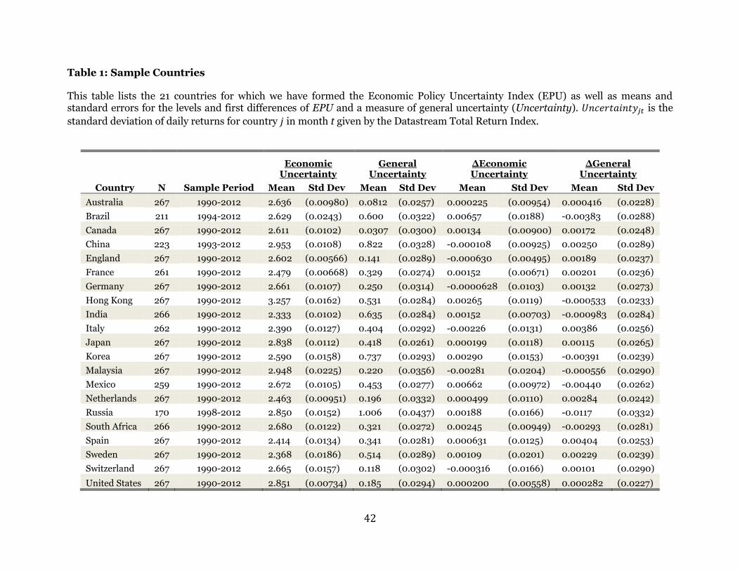
42

Table 1: Sample Countries This table lists the 21 countries for which we have formed the Economic Policy Uncertainty Index (EPU) as well as means and standard errors for the levels and first differences of EPU and a measure of general uncertainty (Uncertainty). is the

standard deviation of daily returns for country in month t given by the Datastream Total Return Index.

Economic

Uncertainty General

Uncertainty ∆Economic Uncertainty

∆General Uncertainty

Country N Sample Period Mean Std Dev Mean Std Dev Mean Std Dev Mean Std Dev

Australia 267 1990-2012 2.636 (0.00980) 0.0812 (0.0257) 0.000225 (0.00954) 0.000416 (0.0228)

Brazil 211 1994-2012 2.629 (0.0243) 0.600 (0.0322) 0.00657 (0.0188) -0.00383 (0.0288)

Canada 267 1990-2012 2.611 (0.0102) 0.0307 (0.0300) 0.00134 (0.00900) 0.00172 (0.0248)

China 223 1993-2012 2.953 (0.0108) 0.822 (0.0328) -0.000108 (0.00925) 0.00250 (0.0289)

England 267 1990-2012 2.602 (0.00566) 0.141 (0.0289) -0.000630 (0.00495) 0.00189 (0.0237)

France 261 1990-2012 2.479 (0.00668) 0.329 (0.0274) 0.00152 (0.00671) 0.00201 (0.0236)

Germany 267 1990-2012 2.661 (0.0107) 0.250 (0.0314) -0.0000628 (0.0103) 0.00132 (0.0273)

Hong Kong 267 1990-2012 3.257 (0.0162) 0.531 (0.0284) 0.00265 (0.0119) -0.000533 (0.0233)

India 266 1990-2012 2.333 (0.0102) 0.635 (0.0284) 0.00152 (0.00703) -0.000983 (0.0284)

Italy 262 1990-2012 2.390 (0.0127) 0.404 (0.0292) -0.00226 (0.0131) 0.00386 (0.0256)

Japan 267 1990-2012 2.838 (0.0112) 0.418 (0.0261) 0.000199 (0.0118) 0.00115 (0.0265)

Korea 267 1990-2012 2.590 (0.0158) 0.737 (0.0293) 0.00290 (0.0153) -0.00391 (0.0239)

Malaysia 267 1990-2012 2.948 (0.0225) 0.220 (0.0356) -0.00281 (0.0204) -0.000556 (0.0290)

Mexico 259 1990-2012 2.672 (0.0105) 0.453 (0.0277) 0.00662 (0.00972) -0.00440 (0.0262)

Netherlands 267 1990-2012 2.463 (0.00951) 0.196 (0.0332) 0.000499 (0.0110) 0.00284 (0.0242)

Russia 170 1998-2012 2.850 (0.0152) 1.006 (0.0437) 0.00188 (0.0166) -0.0117 (0.0332)

South Africa 266 1990-2012 2.680 (0.0122) 0.321 (0.0272) 0.00245 (0.00949) -0.00293 (0.0281)

Spain 267 1990-2012 2.414 (0.0134) 0.341 (0.0281) 0.000631 (0.0125) 0.00404 (0.0253)

Sweden 267 1990-2012 2.368 (0.0186) 0.514 (0.0289) 0.00109 (0.0201) 0.00229 (0.0239)

Switzerland 267 1990-2012 2.665 (0.0157) 0.118 (0.0302) -0.000316 (0.0166) 0.00101 (0.0290)

United States 267 1990-2012 2.851 (0.00734) 0.185 (0.0294) 0.000200 (0.00558) 0.000282 (0.0227)

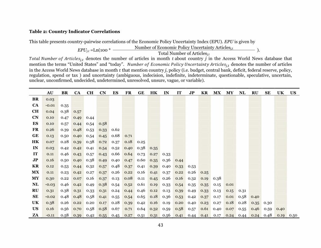
43

Table 2: Country Indicator Correlations This table presents country-pairwise correlations of the Economic Policy Uncertainty Index (EPU). EPU is given by

EPUj,t =Ln(100 * Number of Economic Policy Uncertainty Articlesj,t ).

Total Number of Articlesj,t denotes the number of articles in month about country j in the Access World News database that

mention the terms “United States” and “today”. denotes the number of articles

in the Access World News database in month that mention country j, policy (i.e. budget, central bank, deficit, federal reserve, policy, regulation, spend or tax ) and uncertainty (ambiguous, indecision, indefinite, indeterminate, questionable, speculative, uncertain, unclear, unconfirmed, undecided, undetermined, unresolved, unsure, vague, or variable).

AU BR CA CH CN ES FR GE HK IN IT JP KR MX MY NL RU SE UK US

BR 0.03

CA -0.01 0.35

CH 0.04 0.38 0.57

CN 0.10 0.47 0.49 0.44

ES 0.10 0.57 0.44 0.54 0.58

FR 0.26 0.39 0.48 0.53 0.33 0.62

GE 0.13 0.50 0.40 0.54 0.45 0.68 0.71

HK 0.07 0.28 0.39 0.38 0.72 0.37 0.18 0.25

IN 0.03 0.42 0.42 0.41 0.54 0.52 0.40 0.38 0.35

IT 0.11 0.46 0.43 0.57 0.43 0.66 0.64 0.73 0.27 0.33

JP 0.16 0.50 0.40 0.38 0.49 0.40 0.47 0.60 0.35 0.36 0.44

KR 0.12 0.53 0.44 0.32 0.57 0.48 0.37 0.41 0.39 0.40 0.33 0.53

MX 0.11 0.23 0.42 0.27 0.37 0.26 0.22 0.16 0.41 0.37 0.22 0.26 0.25

MY 0.30 0.22 0.07 0.16 0.37 0.13 0.08 0.11 0.45 0.26 0.16 0.32 0.19 0.38

NL -0.03 0.46 0.42 0.49 0.38 0.54 0.52 0.61 0.19 0.33 0.54 0.35 0.35 0.15 0.01

RU 0.31 0.38 0.31 0.33 0.31 0.24 0.44 0.46 0.12 0.13 0.39 0.49 0.33 0.13 0.15 0.31

SE -0.02 0.48 0.48 0.58 0.41 0.55 0.54 0.65 0.18 0.36 0.53 0.42 0.37 0.17 0.01 0.58 0.40

UK 0.38 0.26 0.22 0.20 0.17 0.28 0.39 0.42 0.16 0.19 0.20 0.40 0.23 0.27 0.18 0.28 0.35 0.30 US 0.16 0.56 0.70 0.58 0.58 0.67 0.71 0.64 0.32 0.59 0.58 0.57 0.61 0.40 0.07 0.55 0.46 0.59 0.40 ZA -0.11 0.58 0.39 0.42 0.55 0.45 0.27 0.51 0.31 0.56 0.41 0.44 0.41 0.17 0.24 0.44 0.24 0.48 0.19 0.50

44

Table 3: Economic Policy Uncertainty and Stock Returns Each dependent variable is the one-month total market return for country j in month t. EPU is the Economic Policy Uncertainty Index, defined in Equation 1. Uncertainty is the standard deviation of the daily market returns for country j in month t. denotes first differences. Subscript t stands for contemporaneous variables, while t-1 denotes a one-month lag. t statistics based on standard errors double-clustered by country and month are given in parentheses. *, **, and *** represent significance at the 10%, 5% and 1% levels, respectively.

(1) (2) (3) (4) (5) (6)

∆EPUt -2.925***

-2.501***

(-2.60)

(-2.62)

∆Uncertaintyt -3.890*** -3.849***

(-5.15) (-5.21)

EPUt

-3.061** -1.747*

(-2.17) (-1.76)

EPUt-1

2.810** 3.230***

(2.30) (3.20)

Uncertaintyt

-5.210*** -5.252***

(-5.56) (-5.78)

Uncertaintyt-1

2.654*** 2.503***

(4.06) (3.92)

Constant 2.028*** 1.361*** 1.982*** 1.875 2.762 -2.307

(37.05) (25.02) (23.13) (0.42) (0.31) (-0.74)

Country Fixed Effects Yes Yes Yes Yes Yes Yes

N 5353 5409 5353 5349 5387 5349

Adj-R2 0.004 0.042 0.046 0.004 0.063 0.068

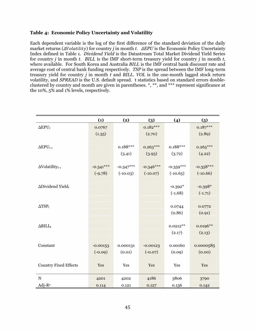
45

Table 4: Economic Policy Uncertainty and Volatility Each dependent variable is the log of the first difference of the standard deviation of the daily market returns ( ) for country j in month t. EPU is the Economic Policy Uncertainty Index defined in Table 1. Dividend Yield is the Datastream Total Market Dividend Yield Series for country j in month t. BILL is the IMF short-term treasury yield for country j in month t, where available. For South Korea and Australia BILL is the IMF central bank discount rate and average cost of central bank funding respectively. TSP is the spread between the IMF long-term treasury yield for country j in month t and BILL. VOL is the one-month lagged stock return volatility, and SPREAD is the U.S. default spread. t statistics based on standard errors double-clustered by country and month are given in parentheses. *, **, and *** represent significance at the 10%, 5% and 1% levels, respectively.

(1) (2) (3) (4) (5)

∆EPUt 0.0767

0.182***

0.187***

(1.35)

(2.70)

(2.89)

∆EPUt-1 0.188*** 0.263*** 0.188*** 0.265***

(3.41) (3.93) (3.72) (4.22)

∆Volatilityt-1 -0.341*** -0.347*** -0.346*** -0.359*** -0.358***

(-9.78) (-10.03) (-10.07) (-10.65) (-10.66)

∆Dividend Yieldt

-0.392* -0.398*

(-1.68) (-1.71)

∆TSPt

0.0744 0.0772

(0.86) (0.91)

∆BILLt

0.0212** 0.0196**

(2.17) (2.13)

Constant -0.00153 0.000131 -0.00123 0.00160 0.0000585

(-0.09) (0.01) (-0.07) (0.09) (0.00)

Country Fixed Effects Yes Yes Yes Yes Yes

N 4201 4202 4186 3806 3790

Adj-R2 0.114 0.121 0.127 0.136 0.142

46

Table 5: Economic Policy Uncertainty and GDP The unit of observation is a quarter t in country j. ∆GDP is the logged first difference of real gross domestic product, ∆Investment is the logged first difference of aggregate real private investment, ∆Consumption is the logged first difference of real personal consumption, and ∆Government is the logged first difference of government expenditures. EPU is the economic policy uncertainty index defined in Table 1. t statistics based on standard errors double clustered by country and month are given in parentheses. *, **, and *** represent significance at the 10%, 5% and 1% levels, respectively.

∆GDP ∆Investment ∆Consumption ∆Government

∆EPUt-1 -0.0672*** -0.125*** -0.0330*** -0.0480

(-3.37) (-4.01) (-2.79) (-1.53)

∆GDPt-1 0.327***

(3.41)

∆Investmentt-1 -0.156*

(-1.96)

∆Consumptiont-1

0.652***

(7.67)

∆Governmentt-1

-0.106

(-1.31)

Constant 0.0161*** 0.0260*** 0.00816*** 0.0283***

(4.69) (5.91) (3.46) (8.48)

N 1578 1522 1522 1522

Adj-R2 0.216 0.090 0.517 0.062

47

Table 6: Economic Policy Uncertainty and the Risk Premium This table presents average excess returns and estimates of abnormal returns for each of the five portfolios formed from sorting on exposure to economic policy uncertainty. Each month m, for

each stock i in CRSP, we form five portfolios sorted on estimated from the following time-

series regressions

( )

Panel A presents average excess returns for these five portfolios. Column 1 (EPU1) reports the results for the most negative stocks, Column 5 for the least negative. Column 6 (EPU1-5) reports the results for the economic policy uncertainty factor-mimicking portfolio, a zero investment portfolio that is long the highest economic policy uncertainty quintile and short the lowest economic policy uncertainty quintile. Panel B presents whole-sample intercepts and

slopes from the Fama-French Three Factors model. That is, for each of the quintiles p, we

estimate the following regression over the entire sample period:

( )

Panel C presents whole-sample estimated intercepts and slopes from the Fama-French Three Factors model augmented with the Carhart (1997) momentum factor (UMD) as well as the Pastor and Stambaugh (2003) Liquidity factor (LIQ):

( )

T statistics are in parentheses.

Panel A: Returns by EPU

EPU1 EPU2 EPU3 EPU4 EPU5 EPU1-5

Return 1.43*** 1.08*** 0.894*** 0.829** 0.8 0.626***

(2.72) (2.86) (2.65) (2.31) (1.64) (3.56)

N 204 204 204 204 204 204

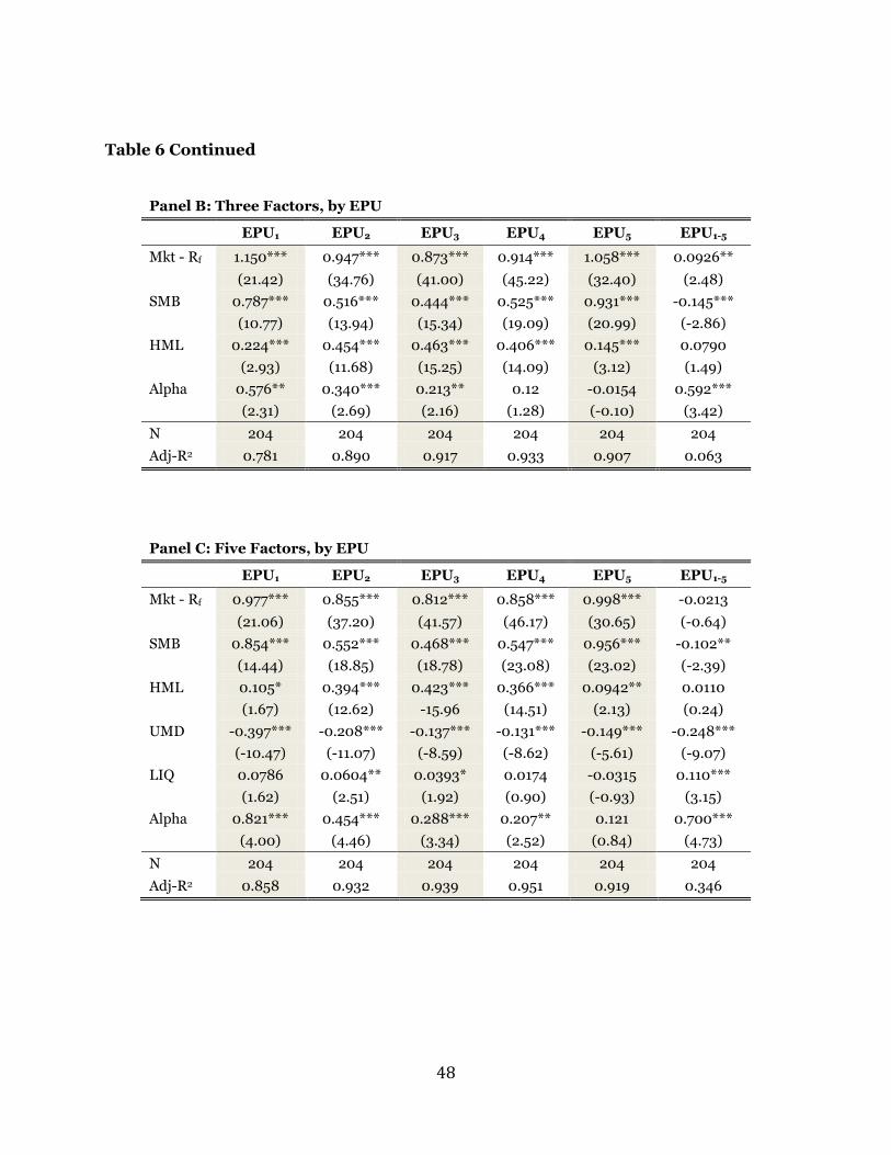
48

Table 6 Continued

Panel B: Three Factors, by EPU

EPU1 EPU2 EPU3 EPU4 EPU5 EPU1-5

Mkt - Rf 1.150*** 0.947*** 0.873*** 0.914*** 1.058*** 0.0926**

(21.42) (34.76) (41.00) (45.22) (32.40) (2.48)

SMB 0.787*** 0.516*** 0.444*** 0.525*** 0.931*** -0.145***

(10.77) (13.94) (15.34) (19.09) (20.99) (-2.86)

HML 0.224*** 0.454*** 0.463*** 0.406*** 0.145*** 0.0790

(2.93) (11.68) (15.25) (14.09) (3.12) (1.49)

Alpha 0.576** 0.340*** 0.213** 0.12 -0.0154 0.592***

(2.31) (2.69) (2.16) (1.28) (-0.10) (3.42)

N 204 204 204 204 204 204

Adj-R2 0.781 0.890 0.917 0.933 0.907 0.063

Panel C: Five Factors, by EPU

EPU1 EPU2 EPU3 EPU4 EPU5 EPU1-5

Mkt - Rf 0.977*** 0.855*** 0.812*** 0.858*** 0.998*** -0.0213

(21.06) (37.20) (41.57) (46.17) (30.65) (-0.64)

SMB 0.854*** 0.552*** 0.468*** 0.547*** 0.956*** -0.102**

(14.44) (18.85) (18.78) (23.08) (23.02) (-2.39)

HML 0.105* 0.394*** 0.423*** 0.366*** 0.0942** 0.0110

(1.67) (12.62) -15.96 (14.51) (2.13) (0.24)

UMD -0.397*** -0.208*** -0.137*** -0.131*** -0.149*** -0.248***

(-10.47) (-11.07) (-8.59) (-8.62) (-5.61) (-9.07)

LIQ 0.0786 0.0604** 0.0393* 0.0174 -0.0315 0.110***

(1.62) (2.51) (1.92) (0.90) (-0.93) (3.15)

Alpha 0.821*** 0.454*** 0.288*** 0.207** 0.121 0.700***

(4.00) (4.46) (3.34) (2.52) (0.84) (4.73)

N 204 204 204 204 204 204

Adj-R2 0.858 0.932 0.939 0.951 0.919 0.346

49

Table 7: Economic Policy Uncertainty and Future Cash Flows The unit of observation is a quarter t in country j. ∆GDP is the logged first difference of real gross domestic product, ∆Investment is the logged first difference of aggregate real private investment, ∆Consumption is the logged first difference of real personal consumption, and ∆Government is the logged first difference of government expenditures. The sample runs from 1990q1 through 2012q1. t statistics based on standard errors double-clustered by country and month are given in parentheses. *, **, and *** represent significance at the 10%, 5% and 1% levels, respectively.

∆GDP ∆Investment ∆Consumption ∆Government

∆EPUt-1 -0.0480** -0.124*** -0.0225 -0.0413

(-2.03) (-3.35) (-1.65) (-1.05)

∆EPUt-2 0.0159 -0.0390 0.00728 -0.0289

(0.72) (-0.98) (0.53) (-0.69)

∆EPUt-3 -0.00882 -0.0619 -0.00620 -0.0144

(-0.34) (-1.53) (-0.40) (-0.30)

∆EPUt-4 0.00481 -0.0175 0.00891 -0.00493

(0.19) (-0.42) (0.51) (-0.10)

∆EPUt-5 -0.0422* -0.0974** -0.0266 -0.0508

(-1.79) (-2.44) (-1.62) (-1.18)

∆EPUt-6 0.0402 0.00599 0.0134 -0.00861

(1.54) (0.13) (0.68) (-0.19)

∆EPUt-7 0.00181 0.00324 0.00334 0.0178

(0.06) (0.08) (0.19) (0.38)

∆EPUt-8 0.0339 0.0498 0.0225 0.0730*

(1.61) (1.42) (1.48) (1.93)

∆GDPt-1 0.347***

(3.14)

∆Investmentt-1 -0.151

(-1.62)

∆Consumptiont-1

0.654***

(6.60)

∆Governmentt-1

-0.120

(-1.32)

Constant 0.0145*** 0.0252*** 0.0225 0.0267***

(4.35) (6.50) (1.48) (9.01)

N 1443 1397 1397 1397

Adj-R2 0.220 0.097 0.512 0.067

50

Table 8: Economic Policy Uncertainty and Cumulative Returns For each country, month pair (j,t) and holding window u (months), denote the cumulative

holding period return over month t through t+u. This table presents estimates of the regressions

where is a set of controls following Ang and Bekaert (2007), Hjalmarsson (2010) and Santa-

Clara and Valkanov (2003). They include Dividend Yield, TSP, BILL, VOL, and SPREAD as defined in Table 4. Each row is a separate regression, with each row in the column Horizon denoting the length of cumulative returns from time t being used as the dependent variable. For each country, the time-series of holding periods overlaps by time periods, so we use Newey-West standard errors with the appropriate bandwidth to account for the resulting autocorrelation (as well as clustering by month to control for cross-sectional correlation). T-statistics are in parentheses to the right of the coefficient. *, **, and *** represent significance at the 10%, 5% and 1% levels, respectively.

Horizon ∆EPUt EPUt-1 Adj-R2

t -2.685** (-2.14) -0.436 (-0.37) 0.011

t+1 -2.938 (-1.43) 0.998 (0.51) 0.020

t+2 -0.914 (-0.44) 2.544 (1.00) 0.025

t+3 -0.773 (-0.32) 2.668 (0.81) 0.034

t+4 -1.616 (-0.55) 3.814 (0.95) 0.048

t+5 -0.655 (-0.21) 5.693 (1.24) 0.060

t+6 0.535 (0.17) 7.963 (1.52) 0.069

t+7 2.291 (0.75) 9.538 (1.54) 0.077

t+8 3.371 (0.89) 10.00 (1.38) 0.081

t+9 3.233 (0.78) 11.27 (1.37) 0.084

t+10 3.276 (0.70) 12.89 (1.44) 0.089

t+11 4.980 (1.01) 15.20 (1.55) 0.093

t+12 5.973 (1.13) 16.72 (1.59) 0.098

t+13 6.393 (1.13) 18.02 (1.60) 0.102

t+14 7.364 (1.22) 20.17* (1.70) 0.107

t+15 8.295 (1.27) 21.85* (1.82) 0.113

t+16 9.867 (1.57) 22.27* (1.87) 0.117

t+17 10.34 (1.56) 21.68* (1.82) 0.120

t+18 9.981 (1.55) 20.42* (1.68) 0.122

t+19 9.373 (1.44) 16.50 (1.31) 0.126

t+20 5.732 (0.81) 13.07 (0.99) 0.129

t+21 4.770 (0.68) 11.71 (0.87) 0.134

t+22 3.674 (0.51) 11.83 (0.85) 0.139

t+23 4.153 (0.55) 13.17 (0.94) 0.143

51

Table 9: Economic Policy Uncertainty and Expected and Unexpected Returns Following Santa-Clara and Valkanov (2003), we decompose cumulative holding period returns into expected and unexpected components to determine their relationships with and EPU. For each country, month pair (j,t) and holding window u (months), denote the cumulative

holding period return over month t to t+u. The expected cumulative holding period return

is formed by taking from the regression

where is the set of controls defined in Table 4. Then, we take the

unexpected holding period return to be [ ]. Panel A presents estimates of the

regression of expected returns on and EPU. Panel B presents estimates of the regressions of unexpected returns on and EPU. Each row is a separate regression, with each row in the column Horizon denoting the length of cumulative returns from time t being used as the dependent variable. For each country, the time-series of holding periods overlaps by time periods so we use Newey-West standard errors with the appropriate bandwidth to account for the resulting autocorrelation (as well as clustering by month). T-statistics are in parentheses to the right of the coefficient. *, **, and *** represent significance at the 10%, 5% and 1% levels, respectively.

Panel A: Expected Return

Panel B: Unexpected Return

Horizon ∆EPUt EPUt-1 Adj-R2

∆EPUt EPUt-1 Adj-R2

t 0.282 (1.53) 0.729*** (3.95) 0.059

-2.807** (-2.20) -0.841 (-0.62) 0.002

t+1 0.674** (2.07) 1.695*** (3.86) 0.071

-3.196 (-1.53) 0.117 (0.05) 0.001

t+2 1.009** (2.23) 2.437*** (3.39) 0.072

-1.571 (-0.72) 0.810 (0.28) -0.003

t+3 1.394** (2.30) 3.357*** (3.16) 0.077

-1.573 (-0.61) 0.575 (0.15) -0.003

t+4 1.972** (2.53) 4.660*** (3.14) 0.082

-2.671 (-0.88) 1.230 (0.28) -0.002

t+5 2.407** (2.50) 5.708*** (2.97) 0.081

-1.922 (-0.60) 2.531 (0.51) -0.002

t+6 2.838** (2.51) 6.792*** (2.91) 0.082

-1.001 (-0.32) 4.033 (0.71) -0.002

t+7 3.285*** (2.60) 7.898*** (2.91) 0.086

0.410 (0.13) 4.883 (0.73) -0.002

t+8 3.689*** (2.62) 8.896*** (2.87) 0.085

1.230 (0.31) 4.769 (0.61) -0.003

t+9 3.970*** (2.60) 9.614*** (2.78) 0.085

0.719 (0.17) 5.122 (0.59) -0.003

t+10 4.435*** (2.69) 10.74*** (2.84) 0.087

0.518 (0.11) 6.114 (0.66) -0.002

t+11 4.642*** (2.62) 11.36*** (2.78) 0.086

1.976 (0.39) 7.635 (0.77) -0.001

t+12 4.891** (2.56) 12.07*** (2.74) 0.083

2.695 (0.50) 8.369 (0.80) -0.001

t+13 5.298*** (2.59) 13.02*** (2.75) 0.082

2.856 (0.50) 8.944 (0.80) -0.001

t+14 5.545*** (2.58) 13.73*** (2.73) 0.082

3.488 (0.57) 9.925 (0.85) -0.000

t+15 5.826*** (2.59) 14.47*** (2.72) 0.083

3.892 (0.58) 10.67 (0.91) 0.000

t+16 6.225*** (2.63) 15.38*** (2.72) 0.082

5.163 (0.80) 10.42 (0.89) -0.001

t+17 6.251** (2.50) 15.53*** (2.58) 0.078

5.411 (0.79) 9.313 (0.79) -0.001

t+18 5.994** (2.28) 15.17** (2.39) 0.075

4.930 (0.74) 7.714 (0.64) -0.003

t+19 6.199** (2.25) 15.71** (2.34) 0.076

4.390 (0.65) 4.148 (0.32) -0.004

t+20 6.132** (2.15) 15.78** (2.24) 0.076

1.025 (0.14) 1.459 (0.11) -0.005

t+21 5.917** (1.99) 15.53** (2.10) 0.077

0.579 (0.08) 0.454 (0.03) -0.005

t+22 5.992* (1.93) 15.77** (2.03) 0.079

-0.506 (-0.06) 0.858 (0.06) -0.005

t+23 6.108* (1.91) 16.08** (2.00) 0.082

-0.100 (-0.01) 2.173 (0.15) -0.004