Embed Size (px)
Citation preview
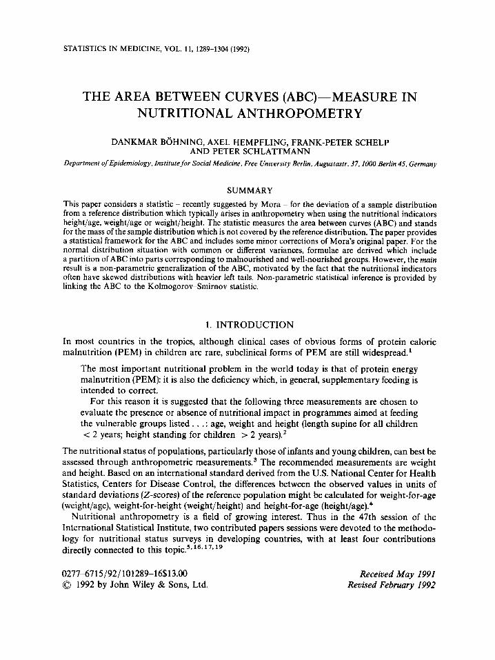
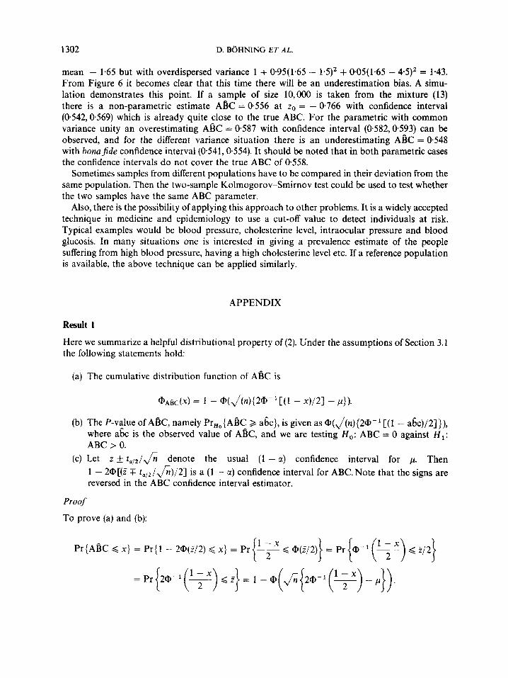
STATISTICS IN MEDICINE, VOL. 11, 1289-1304 (1992)
THE AREA BETWEEN CURVES (ABC)-MEASURE IN NUTRITIONAL ANTHROPOMETRY
DANKMAR BOHNING, AXEL HEMPFLING, FRANK-PETER SCHELP AND PETER SCHLATTMANN
Department of Epidemiology, Institute for Social Medicine. Free University Berlin, Augustastr. 37,1000 Berlin 45, Germany
SUMMARY This paper considers a statistic - recently suggested by Mora - for the deviation of a sample distribution from a reference distribution which typically arises in anthropometry when using the nutritional indicators height/age, weight/age or weight/height. The statistic measures the area between curves (ABC) and stands for the mass of the sample distribution which is not covered by the reference distribution. The paper provides a statistical framework for the ABC and includes some minor corrections of Mora’s original paper. For the normal distribution situation with common or different variances, formulae are derived which include a partition of ABC into parts corresponding to malnourished and well-nourished groups. However, the main result is a non-parametric generalization of the ABC, motivated by the fact that the nutritional indicators often have skewed distributions with heavier left tails. Non-parametric statistical inference is provided by linking the ABC to the Kolmogorov-Smirnov statistic.
1. INTRODUCTION
In most countries in the tropics, although clinical cases of obvious forms of protein calorie malnutrition (PEM) in children are rare, subclinical forms of PEM are still widespread.’
The most important nutritional problem in the world today is that of protein energy malnutrition (PEM): it is also the deficiency which, in general, supplementary feeding is intended to correct.
For this reason it is suggested that the following three measurements are chosen to evaluate the presence or absence of nutritional impact in programmes aimed at feeding the vulnerable groups listed . . . : age, weight and height (length supine for all children < 2 years; height standing for children > 2 years).’
The nutritional status of populations, particularly those of infants and young children, can best be assessed through anthropometric mea~urements.~ The recommended measurements are weight and height. Based on an international standard derived from the U.S. National Center for Health Statistics, Centers for Disease Control, the differences between the observed values in units of standard deviations (Z-scores) of the reference population might be calculated for weight-for-age (weight/age), weight-for-height (weight/height) and height-for-age (height/age).4
Nutritional anthropometry is a field of growing interest. Thus in the 47th session of the International Statistical Institute, two contributed papers sessions were devoted to the methodo- logy for nutritional status surveys in developing countries, with at least four contributions directly connected to this 16, ’’, l9
0277-6715/92/ 101289-16$13.O0 0 1992 by John Wiley & Sons, Ltd.
Received May 1991 Revised February 1992
1290 D. BOHNING ET AL.
Recently Mora6 drew attention to the problems arising from conflicting recommendations about the use of different cut-off points and classification systems. 2-scores are constructed to measure the nutritional status of a child against a reference group of children supposed to be healthy and well nourished. Then a certain value is chosen, also called cut-ofpoint, and children having a Z-score below this cut-off point are considered to be malnourished or undernourished. The percentage of all children in the study population falling below the cut-off point defines the preoalence rate of malnourishment.
Different choices of cut-off values are commonly used (- 1.5, - 2, - 3), which makes the comparison of prevalence estimates difficult. This motivates the search for a measure which is independent of a cut-off value. However, if one is in a diagnostic situation to identify mal- nourished children in order to intervene, the selection of a cut-off value cannot be avoided.
In Mora’s paper6 a method is proposed to estimate the area between the study population density and the density of the reference population. He suggests the term standardized preoalence of malnutrition for this statistic and implies that his approach might be considered to replace the critical choice of cut-off points for prevalence estimates in cross-sectional population studies. The interpretation of the area between curves (ABC) as a measure of the deviation of the nutritional status from the reference population is suggested here and considered to be a helpful tool. A statistical framework for the ABC will be provided.
2. DEFINING NUTRITIONAL STATUS
2.1. Reference populations
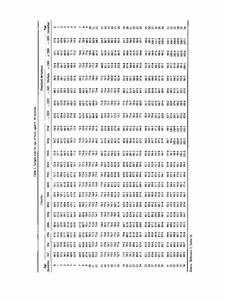
The construction of the 2-scores assumes the availability of so-called reference or standard populations. A reference population is constructed for statistical comparisons, not as a norm for desired body growth. Some criteria for a reference population are that it is well organized, contains detailed information and is internationally available and used. Such a reference popula- tion is provided by the U.S. National Centre for Health Statistics and can be found, for example, in Reference 2. Table I and Table I1 are part of this reference population and are reproduced here for demonstration purposes. For example, Table I refers to the indicator height/age. Here, for each age group various statistical measures of the reference population are given. On the right, we find the median of each age group, as well as median f 1, 2 or 3 SDs. To be more specific, for a boy of 7 months, we find a reference median of 69-5 cm, and median - 2 SD is 64.1 cm. The left part of the table contains various percentiles. The computation of 2-scores involving height is somewhat confused by the fact that the height is measured differently as length (supine length) and stature (measured standing), and overlapping reference populations do exist. Obviously, both forms of computation lead to different height/age values. Which one to follow depends on the form of body height measurement.
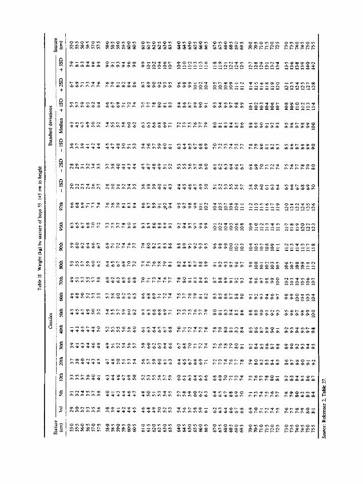
Table I1 contains analogous statistical measures for the reference population referring to the indicator weight/height. Note that this reference population does not involve age. In this case, the grouping variable is body length having an increment of 0.5 cm.
2.2. Construction of Z-scores
Z-scores are constructed to measure the nutritional status of a child against a reference popula- tion of children. The measurements of the group of children under investigation are related to those of the reference with the same age and sex to yield a score independent of the child’s age and sex. Usually, this goal is achieved for sex. With age, one often observes a drop-down effect for the
Tabl
e I.
Leng
th (cm) by a
ge o
f bo
ys a
ged
0-36
mon
ths
Cen
tiles
St
anda
rd d
evia
tions
A
ge
Age
(m
onth
s)
3rd
5th
10th
20
th
30th
40
th
50th
60
th
70th
80
th
90th
95
th
97th
- 3
SD
- 2
SD
- 1
SD
Med
ian
+ 1S
D
+ 2S
D
+ 3SD
(m
onth
s)
0 1 2 3 4 5 6 7 8 9 10
11
12
13
14
15
16
17
18
19
20
21
22
23
24
25
26
27
28
29
30
31
32
33
34
35
36
46.2
46
.7
49.9
50
.5
53.2
53
.9
56.1
56
.8
58.6
59
.3
6@8
61.5
62
.8
63,4
64.5
65
.1
66.0
66
.6
67.4
68
.0
68.7
69
.3
69.9
70
5 71
.0
71.6
72.1
72
.7
73.1
73
.8 74
.1 74
.7
75.0
75
.7
75.9
76
.6
76.7
77.4
77.5
78
.2
78.3
79
.0
79.1
79
.8
79.8
80
.6
806
81.3
81
.3
82.1
82.1
82
.9
82.8
83
.6
83.6
84
.4
84.4
85
.2
85.1
85
.9
85.8
86
.7
86.6
87
.4
87.3
88
.1
88.0
88
.8
88.6
89
.4
89.3
90
.1
89.9
90.7
47.6
51.4
54
.8
57.7
60
.3
62.5
64.4
66 I
67.6
68
.9 70
.2 71
.5 72
.6
73.1
74
.8
75.8
76
.1
77.6
785
79.4
80
.2
81.0
81
.8
82.6
83
.3
84.1
84
.9
85.6
86
4 87
.2
87.9
88.6
89
3 90.0
90.1
91
.4
92.0
48.6
49
.3
52.5
53
.3
55.9
56
.7 58
.9
59.7
61
.4
62.3
63
.6
64.5
65
.6
66.4
67.2
68
.1
68.7
69
.6
70
1
70.9
71
.4
72.2
72
.6
73.5
73
.8
74.7
74.9
75
.8
16.0
76
.9
77.0
71
.9
78.0
78
.9
78.9
79
.9
79.8
80
.8
80.7
81
.7
81.6
82.6
82
.4
83.4
83
.2
84-3
84
.0
85.1
84
.8
85.9
85.6
86
.7
86.4
87
3 87
.1
88.2
87
.9
89.0
88
7 89
.8
89.4
903
90.1
91
.2
90.9
91
.9
91.6
92
.6
92.2
93
.3
92.9
94
.0
93.5
94
.7
49.9
50
.5
53.9
54
.6
57.4
58
.1 60
.4
61.1
63
.0
63.7
65
.2
65.9
67
.1
67.8
68.8
69
.5
703
71.0
71
.7
72.3
73
.0
73.6
74.2
74
.9
15.4
76
.1
76.5
77
.2 77
.6 78
.3
78.7
19
.4
79.7
80
.4
80.7
81
.4
81.6
82
.4
82.6
83
.3
83.4
84
.2
84.3
85
.1
85.2
86
.0
86.0
86
.8
86.8
81
.6
87.6
88
.5
88.4
89
.2
89.2
90.0
89.9
90
.8
90.7
91.6
91
.4
92.3
92.2
93
.0
92.9
93
.7
93.6
94
.5
94.3
95
.2
95.0
95
.8
95.6
96
.5
51.1
51
.7
55.2
55
.9
61.8
62
.5
64.4
65
.1
66.6
67
.3
68.5
69
.2
70.2
70
.9
71.6
72
.4
73.0
73
.7
74.3
75
.0
75.6
76
.3
76.8
77
.5
77.9
18
.7
19.1
79
.8
80.1
80
.9
81.2
82
.0
82.2
83
.0
83.2
84
.0
84.1
85
.0
85.0
85
.9
85.9
86
.8
86.8
87
.7
87.7
88
.6
88.5
89
.4
89.3
90
.2
90.1
91
.0
90.9
91.8
91
.7
92.6
92
.4
93.3
93
.2
94.1
93.9
94
.8
94.6
95
.5
95.3
96
.3
96.0
97
.0
96.7
91
.1
97.4
98
.4
58.7
59
.4
52.4
56
.6
60.2
63
.3
66.0
68.2
10
.1
71.7
73
.2 74
.6
75.9
77
.1
78.4
19.5
80
.7
81.8
82
.9
83.9
85
.0
86.0
86
.9
81.8
88
.7
89.6
90
.5
91.3
92
.1
92.9
93
.7
94.4
95
.2
95.9
96
.6
97.4
98
.1
98.8
99
.5
53.4
51
.7
61.4
64
.5
67.1
69
.4
71.3
72.9
74
.4
75.7
77.0
78.3
79
.5
80.1
81
.9
83.1
84
.2
85.3
86
.3
87.3
88
.3
89.3
90
.2
91.1
92
.0
92.8
93
.6
944
95.2
95
.9
96.7
97.4
98
.2
98.9
99
.6
1003
10
1.0
54.2
58
.6
62.3
65
.5
68.1
70.3
72
.2
73.9
75
.3
76.7
78.0
79
.3
80.5
81.1
82
.9
84.1
85
.2
86.3
81
.4
88.4
89
.5
90.4
91
.4
92.3
93
.2
94.0
94
.9
95.7
96
.4
97.2
91
.9
98.7
99
.4
100.
1 10
0.9
101.
6 10
2.3
54.8
59.2
62
.9
66.1
68
.7
71.0
72
.9
74.5
76
.0
77.3
78
.6
79.9
81
.2
82.4
83
.6
84.8
85
.9
81.0
88
.1
89.2
90
.2
91.2
92
.2
93.1
94
.0
94.8
95
.7
963
97.2
98
.0
98.1
99.5
10
0.2
100.
9 10
1.7
102.
4 10
3.2
43.6
47
.2
504
53.2
55
.6
57.8
59
.8
61.5
63.0
64
.4
65.7
66
.9
68.0
69.0
70.0
70.9
71
.7
723
13.3
74.0
74
.7
15.4
16
. I 76
.8
71.5
78.3
79
.0 79
.8
80.5
81
.3
82.0
82.7
83
.4
84.1
84
.7
85.4
85
.9
45.9
49
.7
52.9
55
.8
58.3
60.5
62
.4
64.1
65
.7
67.0
68
.3
69.6
70.7
71.8
72
.8
13.7
74
.6
15.5
16
.3
77.1
77
.9
18.7
19
.4
80.2
80
.9
81.7
82
.4
83.2
83
.9
84.7
85
.4
86.2
86
.9
87.6
88
.2
88.8
89
.4
48.2
52
.1
55.5
58
3 61
.0
63.2
65
.1
66.8
68.3
69
.7
71.0
72
2 73
.4
74.5
75
.6
76.6
77
.5
78.5
79
.4
80.2
81
.1
81.9
82
.7
833
84.3
85.1
85
.8
86.6
88.1
88
-9
89.6
90.3
91.0
91
.7
92.3
93
.0
87.4
50.5
54
.6
58.1
61
.1
63.7
65
.9
67.8
69.5
71
.0
72.3
73
.6 74
.9 76
.1
77.2
78
.3
79.4
80
.4
81.4
82
.4
83.3
84
.2 85
.1
86.0
86
.8
87.6
883
89.2
900
90.8
91
.6
92.3
93.0
93
.7 94
3 95
.2
95.8
96
.5
52.8
57
.0 M
)7
637
66.4
68
.6 7@
5
72.2
73
.6
75.0
76
.3
77.5
78
,8
8QO
81.1
82
.3
83.4
84
.4
85.4
86.4
81
.4
88.4
89
.3
90.2
91
.0
91.8
92
.7
93.4
94
.2
95.0
95
.7
96.5
97
.2
97.9
98
.6
99.3
10
0.1
55.1
59.5
63
.2
66.4
69
.1
71.3
13
.2
74.8
76
.3
77.6
78
.9
802
81.5
82.7
83
.9
85.1
86
.3
87.4
88
.5
89.5
90
.6
91.6
92
.5
93.5
94
.4
95.2
96
.1
96.9
97
.6
98.4
99
.2
99.9
10
0.6
101.
4 10
2.1
102.
8 10
3.6
57.4
61
.9
65.8
69
.0
71.7
74
.0
75.9
77.5
78
.9
803
81.6
82
.9
84.2
85.5
86
.7
88.0
89.2
9Q
4 91
.5
92.7
93
.8
94.8
95
.8
96.8
97
.7
98.6
99
.5
100.
3 10
1.1
101.
8 10
2.6
103.
3 10
4.1
104.
8 10
5.6
106.
3 10
7.1
0 1 2 3 4 5 6 7 8 9 10
11
12
13
14
15
16
17
18
19
20
21
22
23
24
25
26
27
28
29
30
31
32
33
34
35
36
~~
-~
~~
Sour
ce:
Ref
eren
ce 2
. Tab
le 1
8.
Tabl
e 11
. W
eigh
t (kg) b
y st
atur
e of
boy
s 55
-145
cm
in
heig
ht
Cen
tiles
St
anda
rd d
evia
tions
St
atur
e St
atur
e (c
m)
3rd
5th
10th
20
th
30th
40
th
50th
60
th
70th
80
th
90th
95
th
97th
-
3SD
- 2
SD
- I
SD
Med
ian
+ 1S
D
+ 2SD
+
3SD
(cm)
55.0
55
.5
56.0
56
.5
57.0
57
.5
58.0
58
.5
59.0
59
.5
60.0
60.5
61.0
61
.5
62.0
62
.5
63.0
63
.5
64.0
64.5
65
.0
65.5
66
.0
66.5
67.0
67
.5
68.0
68
.5
69.0
69
.5
70.0
70
.5
71.0
71
.5 72
.0 72
.5
73.0
73
.5
74.0
74
.5
75.0
75
.5
2.9
3.0
3.2
3.3
3.5
3.6
3.8
3.9
4.1
4.2
44
4.
5
4.6
4.8
49
5.0
5.
2 5.
3
5.4
5.6
5.7
58
5
9
6. I
6.2
6.3
6.4
6.6
67
6
8
6.9 7.0
7.1
7.2
7.4
7.5
7.6
7.7
7.8
7.9
8.0
8.1
3.1
32
3.
4 3.5
3.7
3.8
4.0
4.1
43
4.
4 4.
6 4.7
4.8
5.0
51
5.
3 5.4
5.5
5.7
5.8
5.9
6.0
62
6
3
6.4
6.5
6.7
6.8
69
7.
0
7. I
7.3
7.4
7.5
7.6
7.7
7.8
7.9
8.0
8.2
8.3
8.4
3.3
3.5
3.7
3.8
4.0
4.1
4.3
4.4
4.6
4.7
4.9
5.0
5.2
5.3
5.5
5.6
5.7
5.9
6.0
6. I
6.3
64
6
3
6.6
6.8
6.9
7.0
7.1
7,3
7.4
7.5
7.6
7.7
7.8
8.0
8.1
8.2
8.3
8.4
8.5
8.6
8.7
3.7
3.8
4.0
4.2
4.3
4.5
4.7
4.8
5.0
5. I
5.3
5.4
5.6
57
59
6.0
61
6.3
6.4
6.5
6.7
6.8
6.9
7. I
7.2
7.3
7.4
7.6
7.7
7.8
7.9
8.0
8.2
8.3
8.4
8.5
8.6
8.7
8.8
9.0
9.1
9.2
3.9
4.1
4.3
4.4
46
48
4.9
5. I
52
5.4
5.6
5.7
5.9
6.0
6.2
6.3
6.4
6.6
6.7
6.8
7.0
7.1
7.2
7.4
7.5
7.6
7.8
7.9
8.0
8. I
8.2
8.4
8.5
8.6
8.7
8.8
8.9
9.0
9.2
9.3
9.4
9.5
4.1
43
4.
5 4
7
4.8 5.0
5.2
5.3
5.5
5.6
5.8
6.0
6.1
6.3
6.4
6.5
6.7
6.8
7.0
7.1
7.2
74
7.
5 7.
6
7.8
7.9
8.0
8.1
8.3
84
8.5
8.6
8.7
8.9
9.0
9.1
9.2
9.3
9.4
9.5
9.7
9.8
4.3
4.5
4.7
4.9 5.0
5.2
5.4
5.5
5.7
5.9
6.0
6.2
6.3
6.5
6.6
6.8
6.9
7.1
7.2
7.3
7.5
7.6
7.7
7.9
8.0
8. I
8.3
8.4
8.5
8.6
8.8
8.9
9.0
9.1
9.2
9.3
9.5
9.6
9.7
9.8
9.9
10.0
4.6
44
5.0
5.
2 5.
3 5.
5
5.7
5.8
6.0
62
63
6.
5
6.6
6.8
6.9
7.1
7.2
7.4
7.5
7.7
7.8
7.9
8. I
8.2 8.3
8.5
8.6
8.7
8.8
9.0
91
9.
2 9.
3 9.
4 9.
6 9.7
9.8
9.9
10.0
10.1
10.3
10.4
4.9
5.1
5.3
5.5
5.7
5.8
6.0
62
6.3
65
6.
6 6.
8
7.0
7. I
7.3
7.4
7.6
7.7
7.8
8.0
8.1
8.3
8.4
8.5
8.7
8.8
8.9
9.1
9.2
9.3
9.4
9.6
9.7
9.8
9.9
10.0
10.2
10
.3
10.4
10
.5
10.6
10
.7
5.3
55
5.7
5.
9 6.
0 6.
2
6.4
65
6.
7 6
9
7.0
7.2
7.3
7.6
7.8
7.9
8.1
8.2
8.4
8.5
8.7
8.8
8.9
9.1
9.2
9.3
9.5
9.6
9.7
9.8
10.0
10
.1 10
.2
10.3
10
.5
10.6
10
.7
10.8
10
.9
11.1
11
.2
7.5
59
6.
0 6.
2 6.
4 6.
6 6.7
69
7.
I 7.2
7.
4 7.
6 7.7
7.9
80
8.2
8.3
8.5
8.6
8.8 8.9
91
9.
2 9.
3 9.
5
9.6
9.8
9.9
100
10.2
10
.3
10.4
10
.5
10.7
10.8
10
.9 11
.1
11.2
11
.3
11.4
11
.5
11.7
11
.8
6.3
6.5
6.7
6.8
7.0
7.2
7.3
7-5
7.7
7.8
8.0
8.1
8.3
8.5
8.6
8.8
8.9
9.1
9.2
9.4
9.5
9.7
9.8
9.9
10.1
10
.2
10.4
10
.5
10.6
10
8
10.9
I .o
1.2
1.
3 1.4
1.
5 1.7
1.8
11.9
12.0
12
.2
12.3
6.6
6.8
6.9
7.1
7.3
7.4
7.6
7.8
7.9
8.1 8.3
8.4
8.6
8.7
8.9
9.1
9.2 9.4
9.5
9.7
9.8
9.9
10.1
10
.2
10.4
10
.5
10.7
10
.8
10.9
11
.1
11.2
11
.3
11.5
11
.6
11.7
11
.9
12.0
12
.1
12.2
12
.4
12.5
12
.6
20
2.
2 2.
3 2.4
2.
6 2.7
2.8
3.0
3.1
3.2
3.4
3.5
3.6
3.8
3.9
4.0
4. I
4.3
4.4
4.5
4.6
4.7
4.9
5.0
5.1
5.2
5.3
5.5
5.6
5.7
5.8
5.9
6.0
6.1
6.3
6.4
6.5
6.6
6.7
6.8
6.9
7.0
2.8
2.9
3.1
3.2
3.4
3.5
3.7
3.8
4.0
41
4.
3 4.
4
4.5
4.7
4.8
4.9
5.1
5.2
5.3
5.5
5.6
5.7
5.8
6.0
6.1
6.2
6.3
6.4
6.6
67
6.8
6.9 7.0
7.1
7.2
74
7.5
7.6
7.7
7.8
7.9 8.0
3.6
3.7
3.9
4.1
4.2
4.4
4.5
4.7
4.8 5.0 5.1
5.3
5.4
5.6
5.7
5.9
6.0
6.1
6.3
6.4
6.5
67
6.
8 6
9
7.0
7.2
7.3
7.4
7.5
7.7
7.8
7.9
8.0
8.1
8.2
8.3
8.5
8.6
8.7 8.8
8.9
9.0
4.3
4.5
47
4.9
5.0
5.2
5.4
5.5
5.7
5.9
6.0
6.2
6.3
6.5
6.6
6.8
6.9
7.1
7.2
7.3
7.5
7.6
7.7
7.9
8.0
8.1
8.3
8.4
8.5
8.6
8.8 8.9
9.0
9.1
9.2
9.3
9.5
9.6
9.7
9.8
9.9
I00
5.5
5.7
5.9
6.1
6.2
6.4
6.6
67
6.9
7.1
7.
2 7.
4
7.5
1.7
7.8
8.0
8.1
8.3
8.4
8.6
8.7
8.9
90
9.1
9.3
9.4
9.5
9.7
9.8
9.9
10.1
10
.2
10.3
10
.4 10
6 10
.7
10.8
10
9 11
.0
11.2
11
.3
11.4
6.7
69
7.1
7.3
7.4
7.6
7.8
7.9
8.1
8.2
8.4 8.6
8.7
8.9
9.0
9.2
9.3
9.5
9.6
9.8
9.9
10.1
10
2 10
.4
10.5
10
.7
10.8
10
.9
11.1
11
.2
11.4
11
.5
11.6
11
.8
11.9
12
-0
12.1
12
.3
12.4
12
.5
12.7
12
.8
7.9
8.1 8.3
8.4
8.6
8.8
9.0
91
9.
3 9.
4 9.
6 9.8
9.9
101
102
104
106
107
109
11.0
11
.2
11.3
11
.5
11.6
11.8
11
.9
12.1
12
2 12
.4
125
12.7
12
.8
12.9
13
.1
13.2
13
.4
13.5
13
.6
13.8
13
.9
14.0
14
.2
55.0
55
.5
56.0
56
.5
57.0
57
.5
58.0
58
.5
59.0
59
.5
60.0
60
.5
61.0
61
.5
620
623
63.0
63
.5
64.0
64
.5
65.0
65
.5
66.0
66
.5
67.0
67
.5
68.0
68
.5 69
.0
69.5
700
705
71.0
71.5
72.0
72.5
73.0
73.5
74.0
74.5
75.0
75.5
Sour
ce: R
efer
ence
2, T
able
27.

AREA BETWEEN CURVES (ABC) 1293
Z-scores height/age or weight/age during the first 6 months in data from developing countries.' Here, children are losing the nutritional status provided at birth within the first half-year of life.
Now the three Z-scores under consideration are defined more precisely. In general,
individual's value - median value of ref. pop. standard deviation value of ref. pop.
Z-score =
Thus
H - HA - mWA - mWH ZHA = 9 z W A = 5 z W H = SDHA SDWA SDWH '
where H, Wand A are the child's height, weight, and age, respectively; mHA is the median height in the corresponding age and sex group of the reference population; mWA is the median weight in the corresponding age and sex group of the reference population; mWH is the median weight in the corresponding height and sex group of the reference population; and SDHA, SDWA and SDwH are the corresponding standard deviations of the reference population. Different standard deviations are used in the reference population in connection with weight, since its distribution is skewed. To be more precise, there are two standard deviations, one for values above and one for values below the median. Suppose a boy is of 64.0 cm height. We find the lower standard deviation in Table I1 to be 0.9 kg, whereas the upper standard deviation is 1.2 kg. For the computation of ZWH we have to take into consideration the actual weight of the boy. If it is above the median of the reference population, we use 1.2 kg SD; otherwise we use 0.9 kg SD. This is completely analogous for ZwA. To demonstrate the computation with actual values, let us further assume the boy is 6 months old and weighs 5.8 kg. We find the three scores as Z H A = - 1-42, ZWA = - 1.07 and ZWH = - 0.44.
In the setting of a developing country the age of the child is given by the mother and is very often imprecise, leading sometimes to a phenomenon called age heaping,* which means that the Z-score shows the behaviour of a wave if plotted against age. Therefore a Z-score, such as ZWH, not involving age is often preferred. Also, the possible error for ZWA when the age is not entirely correct is usually greater than for ZHA. This is because weight increments are greater than height increments over time in a preschool child.
2.3. Computational aspects
It is clear that the calculation of 2-scores for an individual subject needs great care and, if done by hand, such computations can contain errors. It is therefore advisable whenever possible to use a computer program. Such software is available either in Epi-Infog in a submodule called Measure, or in a program specifically developed by Bohning and Schelp" to compute these scores and which is available on request.
2.4. The choice of cut-off values
The construction of Z-scores (as well as percentiles and median percentages) is done to achieve a measure for the nutritional status of a child. Typically, a low Z-score will indicate malnutrition. The question of a threshold or cut-off value arises and is still under discussion. However, quite frequently values of Z < - 2 are judged to indicate a certain degree of malnutrition. Thus stunted children are defined as those with a Z H A < - 2, and wasted children with a ZWH < - 2. Presently the reasons for stunting are under active discussion, and the former implicit assumption that Z H A represents the nutritional status in the past is no longer internationally accepted; however,
1294 D. BOHNING ET AL.
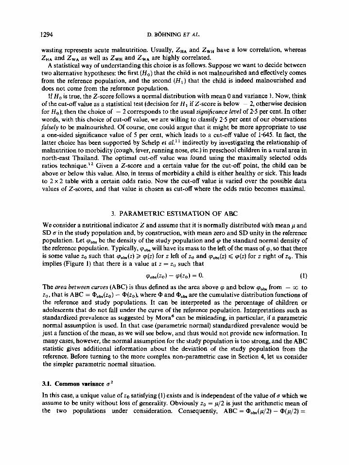
wasting represents acute malnutrition. Usually, ZHA and ZWH have a low correlation, whereas ZHA and ZwA as well as ZWH and ZwA are highly correlated.
A statistical way of understanding this choice is as follows. Suppose we want to decide between two alternative hypotheses: the first (Ho) that the child is not malnourished and effectively comes from the reference population, and the second (HI) that the child is indeed malnourished and does not come from the reference population.
If H o is true, the Z-score follows a normal distribution with mean 0 and variance 1. Now, think of the cut-off value as a statistical test (decision for HI if Z-score is below - 2, otherwise decision for H o ) ; then the choice of - 2 corresponds to the usual Significance level of 2.5 per cent. In other words, with this choice of cut-off value, we are willing to classify 2.5 per cent of our observations falsely to be malnourished. Of course, one could argue that it might be more appropriate to use a one-sided significance value of 5 per cent, which leads to a cut-off value of 1.645. In fact, the latter choice has been supported by Schelp et al.’ indirectly by investigating the relationship of malnutrition to morbidity (cough, fever, running nose, etc.) in preschool children in a rural area in north-east Thailand. The optimal cut-off value was found using the maximally selected odds ratios technique.” Given a Z-score and a certain value for the cut-off point, the child can be above or below this value. Also, in terms of morbidity a child is either healthy or sick. This leads to 2 x 2 table with a certain odds ratio. Now the cut-off value is varied over the possible data values of Z-scores, and that value is chosen as cut-off where the odds ratio becomes maximal.
3. PARAMETRIC ESTIMATION OF ARC
We consider a nutritional indicator Z and assume that it is normally distributed with mean p and SD 0 in the study population and, by construction, with mean zero and SD unity in the reference population. Let (Pobs be the density of the study population and cp the standard normal density of the reference population. Typically, (p& will have its mass to the left of the mass of cp, so that there is some value zo such that cpobs(z) 2 cp(z) for z left of zo and cpobs(z) < cp(z) for z right of zo. This implies (Figure 1) that there is a value at z = zo such that
cpObs(Z0) - cp(Z0) = 0. (1) The area between curves (ABC) is thus defined as the area above cp and below (P&s from - 00 to zo, that is ABC = @obs(zo) - cP(zo), where @ and are the cumulative distribution functions of the reference and study populations. It can be interpreted as the percentage of children or adolescents that do not fall under the curve of the reference population. Interpretations such as standardized prevalence as suggested by Mora6 can be misleading, in particular, if a parametric normal assumption is used. In that case (parametric normal) standardized prevalence would be just a function of the mean, as we will see below, and thus would not provide new information. In many cases, however, the normal assumption for the study population is too strong, and the ABC statistic gives additional information about the deviation of the study population from the reference. Before turning to the more complex non-parametric case in Section 4, let us consider the simpler parametric normal situation.
3.1. Common variance 0’
In this case, a unique value of zo satisfying (1) exists and is independent of the value of 0 which we assume to be unity without loss of generality. Obviously zo = p/2 is just the arithmetic mean of the two populations under consideration. Consequently, ABC = Oobs(p/2) - cP(p/2) =

AREA BETWEEN CURVES (ABC) 1295
0.4
0.3
0.2
0.1
0.0 -3 -2 -1 20
I
z4 1 2
Figure 1. Area between curves (ABC)
cP(p/2 - p) - @(p/2) = @(- p/2) - cP(p/2) = 1 - 2cP(p/2). This can be estimated by
ABC = 1 - 2@(2/2), (2) where 2 is the mean of a sample from the study population. In Result 1 of the Appendix some facts are summarized which are useful for the statistical inference (P-value, confidence interval). For example, a large-sample 95 per cent confidence interval for ABC is given by
1 - 2cP((i & 1*96/&)/2),
that is replacing p in 1 - cP(p/2) by its large-sample confidence interval.
3.2. Different variances u2
In this case there are two solutions, as demonstrated in Figure 2, and equation (1) takes the form
or equivalently,
(1 - a2)zi - 2z0p + p2 - 2a2 h(a) = 0.
This is a quadratic equation in zo with two solutions, (4)
20 = [ p k U J G ] / ( l - U2) , 9l = p2 + 2(a2 - l)ln(a). (5 )
If a2 > 1, as is the case in Figure 2, then the left zero (the one of interest) is given by [ p + a@3/(1 - 02) and (5 ) is always a real root since 2(02 - l)ln(o) is always positive. It

1296
0.4
0.3
0.2
0.1
0.0
ZO first zero
D. BOHNING ET AL.
ABC ova
Legend N(-.5,2)
N(0,l)
20 second zero
Figure 2. The role of different standard deviations: two points of intersection, two areas between the curves
should be noted that the left zero does not necessarily lie between the mean of the study population and the mean of the reference population.
Thus, the ABC is defined as the difference between the area below the density of the study population and the density of the reference population:
ABC = @'obs" + aJ5-W - a2)) - @ U P + a&1/(1 - cZ))
= @([pa + f i ] / ( l - 0 2 ) ) - @([p + af i ] / ( l - 0 2 ) ) . (6) This is the formula from which Table 2 in Mora6 can be reproduced. The associated formula (Reference 6, p. 139) @([pa + f i ] / ( l - 0')) + @([p - af i ] / ( l - a2)) is evidently incorrect. The problem remains to find a point estimate of ABC given in (6). This could be accomplished by simply replacing p and a in (6) by its sample estimates Z and s, where sz is the sample variance. It should be noted, however, that replacing p in (6) by its large-sample 95 per cent confidence interval, namely Z f 1.96s/&, will not provide a 95 per cent confidence interval for ABC, in full generality. It might be called a bonafide interval. Before this question is discussed any further, a different method of inference will be suggested.
3.3. Partitioning the nutritional status
Recall the interpretation of the ABC thus far: it is the percentage of those children in the sample that does not fall under the curve of the reference population. In contrast to the equal variance case, we have a second area, namely to the right of the second zero. This area could again be

AREA BETWEEN CURVES (ABC) 1297
interpreted as a percentage of children which does not fall under the reference density curve. However, these children would be described as well nourished.
In such circumstances it might be consistent to consider a partition of ABC on the following basis. Thus we calculate ABC for the malnourished and well nourished as
ABCbelow = @([pa + ABCabove = @(cp -
- - @ ( [ p + a@1/(1 - a’))
- @([pa - fi1/(1 - a’)), -
and finally
ABCoverall = ABCbelow - ABCabove. (7) The meanings of these measures are clear from Figure 2, in which ABCbelow = 24.8 per cent, ABCabOve = 9 2 per cent and ABCoverall = 15-6 per cent. The first number is reported in Reference 6 (Table 2, p. 138) as the percentage of malnourished children. In our view, only ABCoverall = 15.6 per cent can have this interpretation, leading to quite different numerical estimates. Again, we would stress that this partition will apply only rarely in practical situations and is therefore a theoretical rather than a practical difficulty.
Of more importance is that one might be tempted to ask: how realistic is this case that the standard deviation of the anthropometric indicator deviates drastically from l? Our own experience supports the fact that the observational density deviates more in the direction of non-symmetry.
4. NON-PARAMETRIC ESTIMATION OF ABC
Typically, the empirical distributions of anthropometric indicators such as ZHA or ZWH have heavier left tails. In contrast, the parametric normal density estimator distributes the mass equally under each tail of the distribution, thus providing a biased estimate of ABC.
4.1. Non-parametric formulation
With this motivation in mind, we consider a non-parametric formulation of the problem. Suppose that the density intersecting point zo, the one satisfying (l), is known. Then we could estimate ABC as F(zo) - @(zo), where F is the non-parametric estimator of mobs, namely the empirical distribution function. The problem is the determination of zo! To solve equation (1) we need to have a non-parametric estimator of (Pobs. However, it is not that easy to define the non-parametric density estimator. One way to approach the problem would be to consider non-parametric density estimation via kernels l 3 or semi-parametric density estimation via mixtures of distribu- t i o n ~ . ~ ~ Instead we will see that it is simpler and more promising to follow a different approach. We reformulate (1) as
or equivalently, find the maximum of
A(z) = @obr(Z) -
with respect to z. But the non-parametric estimator of A = QObs - @ is a = F - 0, and ABC is estimated as the maximum of F - @! In other words: given a sample zl, . . . , z, of Z-scores of the

1298 D. BOHNING ET AL.
C 0
0 C 3
t 0
3
.- t
Y-
.- c a 5 I c v)
0
0 n
20 = -0.69
Figure 3. The ABC measure for height/age
study population, we could estimate ABC as
5
Figure 3 shows the empirical distribution function of height/age for 707 preschool children in north-east Thailand. As reference distribution we have plotted the standard normal. The third curve shows the negative difference (implying that the maximum we are searching for is the minimum in the figure) between these two cumulative distributions. The maximum is attained at zo = - 0.69, giving an estimate of ABCnPa' = 0-63. The corresponding parametric estimate is 0.59 (assuming common variance) and 0.61 (assuming different variances). Evidently, the two paramet- ric estimates differ from the non-parametric by 4 per cent and 2 per cent.
4.2. Non-parametric partition of the nutritional status
Clearly, the terms of ABC below, above and overall could be given analogously to Section 3.3. For example, the existence of a second zero could be detected as a minimum of a. Figure 4 shows the situation of Figure 2 in terms of F, is plotted instead of a. Obviously,
and a. Note again that -
ABC:,P,ar, = ABC;fEw - ABC:gie = max &zi) - &zi) + min &zi). l $ i $ n 1 < i < n
Again, from our experience in practical cases, such a partition will not be necessary.

AREA BETWEEN CURVES (ABC) 1299
-5 -4 -3 -2 -1 0 1 2 3 4 5
zo
Figure 4. Area between curves: the role of different standard deviations
4.3. Statistical inference for the non-parametric estimator
It turns out to be surprisingly simple to give a confidence interval for the ABC parameter. Let denote the cumulative distribution function of the study population. Then we have
maxzIDn(z)I = maxzIF(z) - @obs(Z)I.
max,fD,(z)J = max,[F(z) - @(z) - (#&(Z) - @fz))l = rnax,I&z) - A(z)l.
(10)
(1 1)
This is the usual Kolmogorov-Smirnov statistic.' In addition, (10) can be written as
Thus the distribution of (1 1) is known as the Kolmogorov-Smirnov distribution. This implies not only that ABCnPar is a consistent and unbiased estimator of ABC, but also that a (1 - a) confidence band for A(z) can be found as &z) d,, and in particular we find that the (1 - a) confidence interval for ABCnPar as
ABCnPar k d,, (12)
where d, is the (1 - a) percentile of the Kolmogorov-Smirnov distribution. These results are derived in detail in Result 2 in the Appendix.
5. APPLICATION
We are interested in estimating the prevalence of stunting (ZHA) and wasting (ZwH) in preschool children in a region in north-east Thailand. The data stem from an intervention project aimed to improve the nutritional status of all preschool children up to 60 months of age out of six villages

1300 D. BGHNING ET AL.
in the north-east of Thailand. Anthropometric measurements were taken from 707 children every three months over a period of three years and their 2-scores computed. The following data set describes the situation at baseline. For ZHA we find the following descriptive statistics and estimates for ABC (only one stationarity point of 8 corresponding to a maximum):
ABC(stunting) = maxi8(zi) = &z0) = 0.63, zo = - 0.69
95% CI ABC(stunting) f d, = [ 0 5 8 , 0.681 parametric common variance 059 [0.58, 0.621 parametric different variance 0.61 ABC(wasting) = maxi &zi) = 8(zo) = 0.32, zo = - 0.32 95% CI ABC(wasting) f d, = [O-27, 0.373 parametric common variance 0.26 C0.23, 0.293 parametric different variance 0.30.
It can be seen that there is a drastic difference between the parametric ABC estimate of wasting when a common variance is assumed. The difference from the non-parametric ABC estimate is less strong if a different variance is allowed. To judge the possible deviations it might be valuable to mention the corresponding points in Mora.6 He was obviously aware of the issue, since he writes: ‘The frequent skewness in the distributions observed in developing countries may intro- duce some underestimation in the calculations; however, exact estimations applying our method to actual data from nutrition surveys in developing countries showed that the magnitude of the error is negligible (under 10 per cent of the total prevalence)’ (p. 139). What is remarkable is not the fact that there is a bias up to 10 per cent if a parametric normal is assumed (which is also supported by the study above) but rather the opinion that a bias up to 10 per cent is negligible. Mora continues: ‘Although adjusting for skewness in prevalence estimates is theoretically feasible, for practical purposes this would be an unnecessary sophistication.’ It should be pointed out that our non-parametric approach is a simple alternative as well as having the statistical advantages of being always unbiased and providing a valid confidence interval.
6. DISCUSSION
This paper has provided a statistical concept for the area between the density curve of a sample from the study population and the reference population. Statistical inference is provided for both the parametric normal and the non-parametric situation. The question arises as to how much the parametric and non-parametric approaches differ. To answer this, let us assume that 95 per cent of our study population follows a normal distribution with mean - 1.5 and variance 1, and 5 per cent of the population is ‘contaminated’ by a normal distribution with mean - 4.5 and variance 1. This subpopulation could be thought of as a group of children suffering severe malnourish- ment. In other words we are assuming that the study population follows a mixture of two normals:
0.95cp(x + 1.5) + 0*05cp(x + 4.5). (13) If the reference population is again the normal with mean 0 and variance 1 there is a population ABC of 0.558 at zo = - 0.78. In the parametric normal case with common variance it is falsely assumed that the data are coming from a normal with variance 1 and mean 0.95 x (- 1.5) + 005 x ( - 4.5) = - 1.65. From Figure 5 it is clear that the corresponding ABC is larger than the true ABC, leading to an overestimation. In the parametric normal case with different variances it is falsely assumed that the data are coming from a normal, again with

AREA BETWEEN CURVES (ABC)
0.0
1301
/ /
: / ___--- I I / I / I I
0.4
0.3
0.2
0.1
- \ \
\
1
Figure 5. Overestimation of ABC by parametric estimation (common variance) for contaminated normal study popula- tion
0.4
0.3
0.2
0.1
-6 -5 -4 -3 -2 -1
\ \ \ \
\' -
Legend
N ( - 1.65, 1.43)
Mixture
N(0. 1)
---- -- - - - - --
------
Figure 6. Underestimation of ABC by parametric estimation (different variances) for contaminated normal study population
1302 D. BOHNING ET AL.
mean - 1.65 but with overdispersed variance 1 + 0.95(1-65 - 1.5)' + 0-OS(l.65 - 4.5)2 = 1-43. From Figure 6 it becomes clear that this time there will be an underestimation bias. A simu- lation demonstrates this point. If a sample of size 10,OOO is taken from the mixture (13) there is a non-parametric estimate ABC = 0.556 at zo = - 0.766 with confidence interval (0.542,0.569) which is already quite close to the true ABC. For the parametric with common variance unity an overestimating ABC = 0.587 with confidence interval (0582,0.593) can be observed, and for the different variance situation there is an underestimating ABC = 0.548 with bonafide confidence interval (0.541,0.554). It should be noted that in both parametric cases the confidence intervals do not cover the true ABC of 0.558.
Sometimes samples from different populations have to be compared in their deviation from the same population. Then the two-sample Kolmogorov-Smirnov test could be used to test whether the two samples have the same ABC parameter.
Also, there is the possibility of applying this approach to other problems. It is a widely accepted technique in medicine and epidemiology to use a cut-off value to detect individuals at risk. Typical examples would be blood pressure, cholesterine level, intraocular pressure and blood glucosis. In many situations one is interested in giving a prevalence estimate of the people suffering from high blood pressure, having a high cholesterine level etc. If a reference population is available, the above technique can be applied similarly.
APPENDIX
Result 1
Here we summarize a helpful distributional property of (2). Under the assumptions of Section 3.1 the following statements hold:
(a) The cumulative distribution function of ABC is
@*Bc(X) = 1 - @(J(n){2@-"(1 - x)/2] - p} ) .
(b) The P-value of ABC, namely Pr,,(ABC 2 a&), is given as @(J(n){2@-'[(1 - a6c)/2]}), where a6c is the observed value of ABC, and we are testing H,: ABC = 0 against H,: ABC > 0.
(c) Let z _+ ta,2/& denote the usual (1 - a) confidence interval for p. Then 1 - 2@[(Z T tai2/&)/2] is a (1 - a) confidence interval for ABC.Note that the signs are reversed in the ABC confidence interval estimator.
Proof
To prove (a) and (b):

AREA BETWEEN CURVES (ABC) 1303
To prove (c) we note the equivalence of the following statements:
Result 2
Let A(z) = Q0bs(Z) - @(z) and let d(z) = F(z) - @(z) be its pointwise estimate. Also, let d , denote the 1 - a fractile of the Kolmogorov-Smirnov distribution, for example da = @l;S‘(i - a), where mKS is the cumulative distribution function of the Kolmogorov-Smirnov statistic. Then
(a) a = F - @ estimates A unbiasedly and consistently. (b) ABCnPa‘ = max,,&zi) is a consistent estimate of ABC. (c) F(z) - @(z) k d , is a (1 - a) confidence band for @obs(Z) - @(z). (d) ABCnPar k d, = max,,&z) k d , is a (1 - a) confidence interval for ABC =
maxz@obs(Z) - @(z).
Proof
The following three statements are equivalent and hold with probability 1 - a:
maxzIW - @(z) - (@obE(z) - @ @ ) ) I d d, +a - d, G F ( Z ) - @(Z) - (mobs(Z) - @(Z)) d d,
+*E’(Z) - @(Z) - d, ,< Bobs(Z) - @(Z) < F ( Z ) - @(Z) + d,
for d l Z
for all Z.
The last statement holds for all z, and thus it is true also for the maximum:
max,[F(z) - @(z) - d,] < max,[@ob,(z) - @(z)l d max,CF(z) - @(z) + da]. 0
ACKNOWLEDGEMENTS
This work is supported by the German Research Foundation under various grants. Part of this work was completed while the first author was visiting the Faculty of Tropical Medicine and the Department of Biostatistics, School of Public Health, Mahidol University, Bangkok with support from the German Academic Exchange Service (DAAD). He would like to express his thanks to the faculty for their support during his stay.
REFERENCES
1. United Nations Administrative Committee on Coordination, Subcommittee on Nutrition (UN ACCISCN). Update on the Nutrition Situation. Recent Trends in Nutrition in 33 Countries, ACC/SCN Secretariat, Geneva, 1989.
2. World Health Organization. Measuring Change in Nutritional Status, WHO, Geneva, 1983. 3. Keller, W., Donoso, G. and De Maeyer, E. M. ‘Anthropometry in nutritional surveillance: a review
based on nutritional anthropometry’, Nutrition Abstracts and Reviews, 46, 591-609 (1976). 4. Waterlow, J. C., Buzina, R., Keller, W., Lane, J. M., Nichaman, M. Z. and Tanner, J. M. ‘The
presentation and use of height and weight data for comparing the nutritional status of groups of children under the age of 10 years’, Bulletin ofthe World Health Organization, 55, 489-498 (1977).

1304 D. BOHNING ET AL.
5. Carlson, B. A. ‘Assessing the nutritional status of young children: how to do it with national household sample surveys: a methodological overview’, Bulletin of the International Statistical Institute, Contrib- uted Papers of the 47th Session, I , 183-184 (1989).
6. Mora, J. 0. ‘A new method for estimating a standardized prevalence of child malnutrition from anthropometric indicators’, Bulletin of the World Health Organization, 67, 133-142 (1989).
7. Wolff, M. C., Perez, L., Gibson, J. G., Lopez, L. S., Peniston, B. and Wolff, M. M. ‘Nutritional status of children in the health district of Cusco, Peru’, The American Journal of Clinical Nutrition, 42, 531-541 (1985).
8. Heitjan, D. F. and Rubin, D. B. ‘Inference from coarse data via multiple imputation with application to age heaping’, Journal of the American Statistical Association, 85, 304-314 (1990).
9. Dean, A. D., Dean, J. A., Burton, A. H. and Dicker, R. C. Epi Info, Version 5: a Word Processing, Database, and Statistics Program for Epidemiology on microcomputers, U S D Incorporated, Stone Mountain, Georgia, 1990.
10. Bohning, D. and Schelp, F.-P. ‘A FORTRAN subroutine for computing indicators of the nutritional status of children and adolescents’, Statistical Papers, 27, 141-150 (1985).
11. Schelp, F.-P., Sormani, S., Pongpaew, P., Vudhivai, N., Egormaiphol, S. and Bohning, D. ‘Seasonal variation of wasting and stunting in preschool children during a three-year community-based nutri- tional intervention study in northeast Thailand’, Tropical Medicine and Parasitology, 41, 279-285 (1990).
12. Miller, R. and Siegmund, D. ‘Maximally selected X2-statistics’, Biometrics, 38, 101 1-1016 (1982). 13. Thisted, R. A. Elements of Statistical Computing, Chapman and Hall, London, 1988. 14. Titterington, D. M., Smith, A. F. M. and Makov, U. E. Statistical Analysis of Finite Mixture Distribu-
tions, Wiley, New York, 1985. 15. Mood, A. M., Graybill, F. A. and Boes, D. C. Introduction to the Theory of Statistics, 3rd edn,
McGraw-Hill, New York, 1974. 16. Baker, S. K., Duran-Bordier, A. and Mahamadou, 0. ‘Rapid nutritional assessment in Niger: a practical
approach’, Bulletin of the International Statistical Institute, Contributed Papers of the 47th Session I ,
17. Gorstein, J. and Pradilla, A. ‘Interpreting anthropometric measures-issues of standardization in analysis and presentation’, Bulletin of the International Statistical Institute, Contributed Papers of the 47th Session I , 389-390 (1989).
91-92 (1989).
18. Lindgren, B. W. Statistical Theory, 3rd Edition, Macmillan Publishing Co., New York, 1976. 19. Rutstein, S. and Sommerfelt, E. ‘The nutritional status of small children: methods and results from the
demographic and health surveys’, Bulletin of the International Statistical Institute, Contributed Papers of the 47th Session 11, 278 (1989).