Embed Size (px)
Citation preview

THE APPLICATION OF MULTIWAVELET FILTER BANKS TO
IMAGE PROCESSING∗
V. Strela†,‡, P. N. Heller‡, G. Strang†, P. Topiwala§, C. Heil¶
Abstract
Multiwavelets are a new addition to the body of wavelet theory. Realizable as matrix-valued filterbanks leading to wavelet bases, multiwavelets offer simultaneous orthogonality, symmetry, and shortsupport, which is not possible with scalar 2-channel wavelet systems. After reviewing this recentlydeveloped theory, we examine the use of multiwavelets in a filter bank setting for discrete-time sig-nal and image processing. Multiwavelets differ from scalar wavelet systems in requiring two or moreinput streams to the multiwavelet filter bank. We describe two methods (repeated row and approx-imation/deapproximation) for obtaining such a vector input stream from a one-dimensional signal.Algorithms for symmetric extension of signals at boundaries are then developed, and naturally inte-grated with approximation-based preprocessing. We describe an additional algorithm for multiwaveletprocessing of two-dimensional signals, two rows at a time, and develop a new family of multiwavelets(the constrained pairs) that is well-suited to this approach. This suite of novel techniques is thenapplied to two basic signal processing problems, denoising via wavelet-shrinkage, and data compres-sion. After developing the approach via model problems in one dimension, we applied multiwaveletprocessing to images, frequently obtaining performance superior to the comparable scalar wavelettransform.
EDICS category: IP 1.6
submitted to IEEE Trans. on Image Processing
Contact address:Peter Niels Heller
Aware, Inc.40 Middlesex Turnpike
Bedford, MA 01730-1432Phone: (617) 276-4000
FAX: (617) 276-4001email: [email protected]
∗Work at Aware, Inc. was supported in part by the Advanced Research Projects Agency of the Department of Defenseand monitored by the Air Force Office of Scientific Research under contract no. F49620-92-C-0054. Portions of this workwere performed at the MITRE Corporation with the support of the MITRE Sponsored Research Project.
†Dartmouth College, Hanover, NH 03755‡Aware Inc., Bedford, MA 01730§Sanders, Inc., Nashua, NH 03061¶Georgia Institute of Technology, Atlanta, GA 30332
1

1 Introduction
Wavelets are a useful tool for signal processing applications such as image compression and denoising.
Until recently, only scalar wavelets were known: wavelets generated by one scaling function. But one
can imagine a situation when there is more than one scaling function [16]. This leads to the notion of
multiwavelets, which have several advantages in comparison to scalar wavelets [36]. Such features as
short support, orthogonality, symmetry, and vanishing moments are known to be important in signal
processing. A scalar wavelet cannot possess all these properties at the same time [35]. On the other
hand, a multiwavelet system can simultaneously provide perfect reconstruction while preserving length
(orthogonality), good performance at the boundaries (via linear-phase symmetry), and a high order of
approximation (vanishing moments). Thus multiwavelets offer the possibility of superior performance
for image processing applications, compared with scalar wavelets.
We describe here novel techniques for multirate signal processing implementations of multiwavelets,
and present experimental results for the application of multiwavelets to signal denoising and image
compression. The paper is organized as follows. Section 2 reviews the definition and construction of
continuous-time multiwavelet systems, and Section 3 describes the connection between multiwavelets
and matrix-valued multirate filterbanks. In Section 4 we develop several techniques for applying multi-
wavelet filter banks to one-dimensional signals, including approximation-based preprocessing and sym-
metric extension for finite-length signals. Two-dimensional signal processing offers a new set of problems
and possibilities for the use of multiwavelets; we discuss several methods for the two-dimensional setting
in Section 5, including a new family of multiwavelets, the constrained pairs. Finally, in Section 6 we
describe the results of our application of multiwavelets to signal denoising and data compression.
2 Multiwavelets — several wavelets with several scaling functions
As in the scalar wavelet case, the theory of multiwavelets is based on the idea of multiresolution analysis
(MRA). The difference is that multiwavelets have several scaling functions. The standard multiresolution
has one scaling function φ(t):
• The translates φ(t − k) are linearly independent and produce a basis of the subspace V0;
• The dilates φ(2jt − k) generate subspaces Vj, j ∈ Z, such that
· · · ⊂ V−1 ⊂ V0 ⊂ V1 ⊂ · · · ⊂ Vj ⊂ · · ·
∞⋃
j=−∞Vj = L2(R),
∞⋂
j=−∞Vj = {0} .
2

0.25 0.5 0.75 1 1.25 1.5 1.75 2
-1
-0.5
0
0.5
1
1.5
2
2.5
3
0.25 0.5 0.75 1 1.25 1.5 1.75 2
-1
-0.5
0
0.5
1
1.5
2
2.5
3
Figure 1: Geronimo–Hardin–Massopust pair of scaling functions.
0.25 0.5 0.75 1 1.25 1.5 1.75 2
-3
-2
-1
0
1
2
3
0.25 0.5 0.75 1 1.25 1.5 1.75 2
-3
-2
-1
0
1
2
3
Figure 2: Geronimo–Hardin–Massopust multiwavelets.
• There is one wavelet w(t). Its translates w(t − k) produce a basis of the “detail” subspace W0 to
give V1:
V1 = V0 ⊕ W0.
For multiwavelets, the notion of MRA is the same except that now a basis for V0 is generated by translates
of N scaling functions φ1(t − k), φ2(t − k), . . . , φN(t − k). The vector Φ(t) = [φ1(t), . . . , φN (t)]T , will
satisfy a matrix dilation equation (analogous to the scalar case)
Φ(t) =∑
k
C[k]Φ(2t − k). (1)
The coefficients C[k] are N by N matrices instead of scalars.
Associated with these scaling functions are N wavelets w1(t), . . . , wN(t), satisfying the matrix wavelet
equation
W (t) =∑
k
D[k]Φ(2t− k). (2)
Again, W (t) = [w1(t), . . . , wN(t)]T is a vector and the D[k] are N by N matrices.
As in the scalar case, one can find the conditions of orthogonality and approximation for multiwavelets
[36, 37, 20, 29]; this is discussed below.
A very important multiwavelet system was constructed by J. Geronimo, D. Hardin, and P. Massopust
[16] (see [1] for another early multiwavelet construction). Their system contains the two scaling functions
3

φ1(t), φ2(t) shown in Figure 1 and the two wavelets w1(t), w2(t) shown in Figure 2. The dilation and
wavelet equations for this system have four coefficients:
Φ(t) =
[
φ1(t)φ2(t)
]
= C[0]Φ(2t) + C[1]Φ(2t − 1) + C[2]Φ(2t− 2) + C[3]Φ(2t− 3) ,
C[0] =
3
5
4√
2
5
−1
10√
2−
3
10
, C[1] =
3
50
9
10√
21
,
C[2] =
0 0
9
10√
2−
3
10
, C[3] =
0 0
−1
10√
20
; (3)
W (t) =
[
w1(t)
w2(t)
]
= D[0]Φ(2t) + D[1]Φ(2t− 1) + D[2]Φ(2t− 2) + D[3]Φ(2t− 3) ,
D[0] =1
10
−1√2
−3
1 3√
2
, D[1] =1
10
9√2
−10
−9 0
,
D[2] =1
10
9√2
−3
9 −3√
2
, D[3] =1
10
−1√2
0
−1 0
. (4)
There are four remarkable properties of the Geronimo-Hardin-Massopust scaling functions:
• They each have short support (the intervals [0, 1] and [0, 2]).
• Both scaling functions are symmetric, and the wavelets form a symmetric/antisymmetric pair.
• All integer translates of the scaling functions are orthogonal.
• The system has second order of approximation (locally constant and locally linear functions are in
V0).
Let us stress that a scalar system with one scaling function cannot combine symmetry, orthogonality,
and second order approximation. Moreover, a solution of a scalar dilation equation with four coefficients
is supported on the interval [0, 3]!
Other useful orthogonal multiwavelet systems with second order approximation are the symmetric
pair determined by three coefficients
C[0] =
0 2+√
74
0 2−√
74
, C[1] =
34
14
14
34
, C[2] =
2−√
74 0
2+√
74 0
4

and the Chui-Lian pair [6] determined by the coefficients
C[0] =
12 −1
2
√7
4 −√
74
, C[1] =
2 0
0 1
, C[2] =
12
12
−√
74 −
√7
4
. (5)
Corresponding scaling functions are shown in Figures 3 and 4. Observe that for the symmetric pair
one scaling function is the reflection of the other about its center point. Moreover, the Chui-Lian
symmetric/antisymmetric scaling functions are the sum and difference of the two functions from the
symmetric pair. In this article we will make use of several other nonsymmetric multiwavelets with
desirable properties. More on the construction of multiscaling functions and multiwavelets can be found
in [1, 9, 13, 18, 22, 24, 30, 31, 38, 39, 41].
0.5 1 1.5 2
-0.5
0.5
1
1.5
2
2.5
3
0.5 1 1.5 2
-0.5
0.5
1
1.5
2
2.5
3
Figure 3: Symmetric pair of orthogonal scaling functions.
0.5 1 1.5 2
-0.25
0.25
0.5
0.75
1
1.25
0.5 1 1.5 2
-1.5
-1
-0.5
0.5
1
1.5
Figure 4: Chui-Lian symmetric/antisymmetric orthogonal scaling functions.
5

3 Multiwavelets and multirate filter banks
Corresponding to each multiwavelet system is a matrix-valued multirate filter bank [15], or multifilter. A
multiwavelet filter bank [36] has “taps” that are N ×N matrices (in this paper, we will be working with
N = 2). Our principal example is the 4-coefficient symmetric multiwavelet filter bank whose lowpass
filter was reported in [16]. This filter is given by the four 2 × 2 matrices C[k] of equation (3). Unlike
a scalar 2-band paraunitary filter bank, the corresponding highpass filter (specified by the four 2 × 2
matrices D[k] of equation (4)) cannot be obtained simply as an “alternating flip” of the lowpass filter;
the wavelet filters D[k] must be designed [36]. The resulting 2-channel, 2× 2 matrix filter bank operates
on two input data streams, filtering them into four output streams, each of which is downsampled by
a factor of 2. This is shown in Figure 5. Each row of the multifilter is a combination of two ordinary
filters, one operating on the first data stream and the other operating on the second. For example, the
first lowpass multiwavelet filter given in (3) operates as c0,0[k] on the first input stream and c0,1[k] on
the second. It is a combination of the Haar filter {1, 1} on the first stream and the unit impulse response
on the second stream.
��
�
��
��
��
��
�
D ↓ 2
��
�
��
�
D ↓ 2
C ↓ 2�
��
��
�C ↓ 2
Figure 5: A multiwavelet filter bank, iterated once.
We ask that the matrix filter coefficients satisfy the orthogonality (“block-paraunitarity”) condition
N−1∑
k=0
C[k] C[k − 2l]T = 2δ0,l I . (6)
In the time domain, filtering followed by downsampling is described by an infinite lowpass matrix with
double shifts:
L =
. . .C[3] C[2] C[1] C[0] 0 0
0 0 C[3] C[2] C[1] C[0]. . .
.
Each of the filter taps C[k] is a 2×2 matrix. The eigenvalues of the matrix L are critical. The solution to
the matrix dilation equation (1) is a two-element vector of scaling functions Φ(t) = [φ1(t), φ2(t)]T . The
6

span of integer translates of the multiwavelet scaling functions is the “lowpass” space V0, the set of scale-
limited signals [17]. Any continuous-time function f(t) in V0 can be expanded as a linear combination
f(t) =∑
n
v(0)1,n φ1(t − n) + v
(0)2,n φ2(t − n) .
The superscript (0) denotes an expansion “at scale level 0.” f(t) is completely described by the sequences{
v(0)1,n
}
,{
v(0)2,n
}
. Given such a pair of sequences, their coarse approximation (component in V−1) is
computed with the lowpass part of the multiwavelet filter bank:
...
v(−1)1,n
v(−1)2,n
v(−1)1,n+1
v(−1)2,n+1
...
= L
...
v(0)1,n
v(0)2,n
v(0)1,n+1
v(0)2,n+1
...
.
Because the multifilter C[k] is FIR, each apparently infinite sum in the matrix multiplication is actually
finite and well-defined. Analogously, the details w(−1)1,n , w
(−1)2,n in W−1 are computed with the highpass
part D[k]. Thus the multiwavelet filter bank plays the same mediating role in multiresolution analysis
that a scalar filter bank plays for scalar wavelet systems. If the matrix L has eigenvalues 1, 12 , . . . , 1
2p−1
and the corresponding eigenvectors have a special form, then polynomials of degree less than p belong
to the space V0 [20, 29]. This holds for the Geronimo-Hardin-Massopust multiwavelet filter with p = 2;
linear functions can be exactly represented as linear combinations of integer translates of the scaling
functions φ1 and φ2.
4 One-dimensional signal processing with multiwavelet filter banks
The lowpass filter C and highpass filter D consist of coefficients corresponding to the dilation equation
(1) and wavelet equation (2). But in the multiwavelet setting these coefficients are n by n matrices, and
during the convolution step they must multiply vectors (instead of scalars). This means that multifilter
banks need n input rows. We will consider several ways to produce those rows. In this section the signals
are one-dimensional; in the next section we consider two-dimensional signal processing.
4.1 Oversampled scheme
The most obvious way to get two input rows from a given signal is to repeat the signal. Two identical
rows go into the multifilter bank. This procedure, which we call “repeated row,” is shown in Figure 6. It
7

introduces oversampling of the data by a factor of two. Oversampled representations have proven useful
in feature extraction; however, they require more calculation than critically-sampled representations.
Furthermore, in data compression applications, one is seeking to remove redundancy, not increase it. In
the case of one-dimensional signals the “repeated row” scheme is convenient to implement, and our ex-
periments on denoising of one-dimensional signals were encouraging (see Section 6.1). In two dimensions
the oversampling factor increases to four, limiting the usefulness of this scheme to applications such as
denoising which do not require critically-sampled or near-critically-sampled representation of the data.
��
� �
��
� �
��
� �
��
� �
C
D
↓ 2
↓ 2
x
x
x
Figure 6: Multiwavelet filter bank with “repeated row” inputs.
4.2 A critically-sampled scheme: approximation-based preprocessing
A different way to get input rows for the multiwavelet filter bank is to preprocess the given scalar signal
f [n]. For data compression, where one is trying to find compact transform representations for a dataset,
it is imperative to find critically sampled multiwavelet transform schemes. We describe a preprocessing
algorithm based on the approximation properties of the continuous-time multiwavelets which yields a
critically sampled signal representation. We develop this scheme (suggested to us by J. Geronimo) in the
context of Geronimo-Hardin-Massopust multiwavelets; however, it works equally well for the Chui-Lian
multiwavelets with minor modifications.
Let the continuous-time function f(t) belong to the scale-limited subspace V0 generated by translates
of the GHM scaling functions. This means that f(t) is a linear combination of translates of those
functions:
f(t) =∑
n
v(0)1,n φ1(t − n) + v
(0)2,n φ2(t − n) . (7)
Suppose that the input sequence f [n] contains samples of f(t) at half integers:
f [2n] = f(n), f [2n + 1] = f(n + 1/2).
φ1(t) vanishes at all integer points. φ2(t) is nonzero only at the integer 1. Sampling the relation (7) at
8

integers and half integers gives
f [2n] = φ2(1) v(0)2,n−1 ,
f [2n + 1] = φ2(3/2) v(0)2,n−1 + φ1(1/2) v
(0)1,n + φ2(1/2) v
(0)2,n.
(8)
The coefficients v(0)1,n, v
(0)2,n can be easily found from (8):
v(0)1,n = φ2(1)f [2n+1]−φ2(1/2)f [2n+2]−φ2(3/2)f [2n]
φ2(1)φ1(1/2) ,
v(0)2,n = f [2n+2]
φ2(1) .
Taking into account the symmetry of φ2(t), we finally get
v(0)1,n = φ2(1)f [2n+1]−φ2(1/2)(f [2n+2]+ f [2n])
φ2(1)φ1(1/2) ,
v(0)2,n = f [2n+2]
φ2(1) .(9)
The relations (9) give a natural way to get two input rows v(0)1,n, v
(0)2,n starting from a given signal f [n].
To synthesize the signal on output we invert (9) and recover (8). This sequence of operations is depicted
in Figure 7.
↓ 2
↓ 2
↓ 2
↓ 2
�
����� ���� �
�� �� �
�� �
�� �
�� �
C
D ↓ 2�
�� �
�� �
�� �
�� �
C
D ↓ 2�α0
α1+
z−1z−1
+
Figure 7: Approximation-based preprocessing and two steps of filtering for one-dimensional signals.
In the case of Chui-Lian multiwavelets, the only difference from the above approach is that φ1(1) = 1
and φ2(1) = 0, so that we use the samples of f at the integers to determine the coefficients v(0)1,n and then
find the v(0)2,n from the samples of f at the half-integers.
Given any f(t) ∈ V0, the preprocessing step (9) followed by filtering will produce nontrivial output in
the lowpass branch only. It yields zero output in the highpass subband. For example, f(t) ≡ 1 (locally
in V0) gives v(0)1,n = 1 and v
(0)2,n =
√2, which is the eigenvector of the matrix LT with eigenvalue 1.
This preprocessing algorithm also maintains a critically sampled representation: if the data enters
at rate R, preprocessing yields two streams at rate R/2 for input to the multifilter, which produces four
output streams, each at a rate R/4.
Another advantage of this approximation-based preprocessing method is that it fits naturally with
symmetric extension for multiwavelets (discussed below in Subsection 4.3). In other words, if we sym-
metrically extend a finite length signal f [n] at its boundaries and implement the approximation formulas
(9), then the two rows v(0)1,n, v
(0)2,n from the preprocessor will have the appropriate symmetry.
9

One also can develop a general approximation-type preprocessing based on the following idea. Suppose
again that our given signal f lies in V0. This implies that
f(t) =∑
n,k
v(0)k,n φk(t − n). (10)
The goal of preprocessing is to find the coefficients v(0)k,n from the signal samples.
Assume that a multiwavelet system has N scaling functions, all supported on [0, 1]. Now restrict
equation (10) to this interval:
f(t) =∑
k
v(0)k,0 φk(t) , 0 ≤ t ≤ 1. (11)
Suppose that samples f [0], . . . , f [N − 1] are the values of the function f(t) at the points
t =1
2N,
3
2N, . . . ,
2N − 1
2N.
The representation (11) gives a linear system for the coefficients v(0)0,0, . . . , v
(0)N−1,0. The following N samples
f [N ], . . . , f [2N − 1] give the values of v(0)0,1, . . . , v
(0)N−1,1. Repeating this procedure we find all the v
(0)k,n. If
some of the scaling functions have support longer than [0, 1], we will need several initial (boundary) values
of v(0)k,−1, v
(0)k,−2, . . . . In the case of finite length signals, these numbers can be obtained from the conditions
of periodization or symmetric extension (Section 4.3). Other multiwavelet preprocessing techniques are
discussed in [7, 19, 27, 41, 43, 44, 45, 46].
4.3 Symmetric extension of finite-length signals
In practice all signals have finite length, so we must devise techniques for filtering such signals at their
boundaries. There are two common methods for filtering at the boundary that preserve critical sampling.
The first is circular periodization (periodic wrap) of the data. This method introduces discontinuities at
the boundaries; however, it can be used with almost any filter bank. The second approach is symmetric
extension of the data. Symmetric extension preserves signal continuity, but can be implemented only with
linear-phase (symmetric and/or antisymmetric) filter banks [34, 3, 23, 4]. We now develop symmetric
extension for linear-phase multiwavelet filters, such as the Geronimo-Hardin-Massopust and Chui-Lian
multifilters. This proves useful for image compression applications (Section 6).
Recall the basic problem: given an input signal f [n] with N samples and a linear-phase (symmetric
or antisymmetric) filter, how can we symmetrically extend f before filtering and downsampling in a
way that preserves the critically sampled nature of the system? The possibilities for such an extension
have been enumerated in [4]. Depending on the parity of the input signal (even- or odd-length) and the
parity and symmetry of the filter, there is a specific non-expansive symmetric extension of both the input
signal and the subband outputs. For example, an even-length input signal passed through an even-length
10

symmetric lowpass filter should be extended by repeating the first and last samples, i.e., a half-sample
symmetric signal is matched to a half-sample-symmetric filter. Similarly, when the lowpass filter is of
odd length (whole-sample-symmetry), the input signal should be extended without repeating the first or
last samples.
Each row of the GHM multifilter (equations (3) and (4)) is a linear combination of two filters, one
for each input stream. One filter (applied to the first stream) is of even length; the second is of odd
length. Thus we should extend the first stream using half-sample-symmetry (repeating the first and last
samples) and extend the second stream using whole-sample-symmetry (not repeating samples). Then,
when synthesizing the input signal from the subband outputs, we must symmetrize the subband data
differently depending on whether it is going into an even- or odd-length filter.
In particular suppose we are given two input rows (one of even length, the other of odd length):
v(0)1,0 v
(0)1,1 v
(0)1,2 . . . v
(0)1,N−1
v(0)2,0 v
(0)2,1 v
(0)2,2 . . . v
(0)2,N−1 v
(0)2,N
.
If they are symmetrically extended as
. . . v(0)1,1 v
(0)1,0 v
(0)1,0 v
(0)1,1 . . .
. . . v(0)2,1 v
(0)2,0 v
(0)2,1 v
(0)2,2 . . .
(12)
at the start and. . . v
(0)1,N−2 v
(0)1,N−1 v
(0)1,N−1 . . .
. . . v(0)2,N−1 v
(0)2,N v
(0)2,N−1 . . .
(13)
at the end to give two symmetric rows, then after one step of the cascade algorithm we have the four
symmetric subband outputs:
. . . v(−1)1,1 v
(−1)1,0 v
(−1)1,0 . . . v
(−1)
1, N2−2
v(−1)
1, N2−1
v(−1)
1, N2−1
. . .
. . . v(−1)2,1 v
(−1)2,0 v
(−1)2,1 . . . v
(−1)
2, N2−1
v(−1)
2, N2
v(−1)
2, N2−1
. . .
. . . w(−1)1,1 w
(−1)1,0 w
(−1)1,1 . . . w
(−1)
1, N2−1
w(−1)
1, N2
w(−1)
1, N2−1
. . .
. . . −w(−1)2,1 0 w
(−1)2,1 . . . w
(−1)
2, N2−1
0 −w(−1)
2, N2−1
. . .
The application of the (linear-phase) multiwavelet synthesis filters now yields the symmetric extension
of the original signal.
Multiwavelet symmetric extension can be done not only for linear-phase filters. For example, the
symmetric pair of scaling functions shown in Figure 3 admits the following extension of input data rows
11

v(0)1,k and v
(0)2,k:
. . . v(0)2,1 v
(0)2,0 a v
(0)1,0 v
(0)1,0 v
(0)1,1 . . . v
(0)1,N−1 a v
(0)2,N−1 . . .
. . . v(0)1,1 v
(0)1,0 a v
(0)2,0 v
(0)2,1 v
(0)2,2 . . . v
(0)2,N−1 a v
(0)1,N−1 . . .
.
The placeholder a is an arbitrary real number. After filtering and downsampling of this extended data,
the output rows will have the same symmetry. In this way we obtain a non-expansive transform of
finite-length input data which behaves well at the boundaries under lossy quantization.
4.4 Computational complexity
We briefly compare the computational demands of multiwavelet and scalar wavelet filtering. One level of
the cascade algorithm with the GHM multifilter does require slightly more floating point operations than
the D4 scalar wavelet. General convolution with four 2 by 2 matrix coefficients requires 16 multiplications
and 14 additions to yield two outputs. However, in the case of the GHM multifilter, the presence of
many zero coefficients and the linear-phase symmetry may be exploited to reduce the computation to 8
multiplies and 8 additions for the lowpass filter and 9 multiplications, 11 additions, and 2 sign-flips for
the highpass filter, requiring a total of 17 multiplications, 19 additions, and 2 sign-flips (38 FLOPS total)
for four output values. This amounts to 4.25 multiplications and 9.5 FLOPS per output, compared with
4 multiplications and 7 FLOPS per output for the D4 scalar wavelet filter and 2.5 multiplications and 5.5
FLOPS for the (3,5)-tap linear-phase scalar wavelet of LeGall and Tabatabai. These complexity figures
do not take into account the approximation/deapproximation processing, if any.
5 Two-dimensional signal processing with multiwavelet filter banks
Multiwavelet filtering of images needs two-dimensional algorithms. One class of such algorithms is
derived simply by taking tensor products of the one-dimensional methods described in the previous
section. Another class of algorithms stems from using the matrix filters of the multiwavelet system for
fundamentally two-dimensional processing. We discuss each of these alternatives now.
5.1 Separable schemes based on one-dimensional methods
Section 4 described two different ways to decompose a one-dimensional signal using multiwavelets. Each
of these can be turned into a two-dimensional algorithm by taking a tensor product, i.e., by performing
the 1D algorithm in each dimension separately.
Suppose our 2D data is represented as an N by N matrix I0. The first step is to preprocess all the
rows and store the result as a square array I1 such that the first half of each row contains coefficients
corresponding to the first scaling function and the second half contains coefficients corresponding to the
12

second scaling function. The next operation is preprocessing of the columns of the array I1 to produce
an output matrix I2, such that the first half of each column of I2 contains coefficients corresponding to
the first scaling function and the second half of each column corresponds to the second scaling function.
Then the multiwavelet cascade starts – it consists of iterative low and high-pass filtering of the scaling
coefficients in horizontal and vertical directions. The result after one cascade step can be realized as the
following matrix:L1L1 L2L1 H1L1 H2L1
L1L2 L2L2 H1L2 H2L2
L1H1 L2H1 H1H1 H2H1
L1H2 L2H2 H1H2 H2H2
Here a typical block H2L1 contains low-pass coefficients corresponding to the first scaling function in
the horizontal direction and high-pass coefficients corresponding to the second wavelet in the vertical
direction. The next step of the cascade will decompose the “low-low-pass” submatrixL1L1 L2L
L1L2 L2L2in
a similar manner.
As noted before, the separable product of one-dimensional “repeated row” algorithms leads to a 4:1
data expansion, restricting the utility of this approach to applications such as denoising by thresholding,
for which critical sampling is irrelevant. The separable product of the approximation-based preprocessing
methods described in Section 4.2 yields a critically sampled representation, potentially useful for both
denoising and data compression.
5.2 Constrained multiwavelets
A different approach to two-dimensional multiwavelet filtering is to make use of the two-dimensionality
of the matrix filter coefficients. When processing an image with a scalar filterbank one usually uses as
input the rows and columns of the image. For a multiwavelet system we need n input signals. Where
can we get them? The first solution which comes to mind is very simple: just use n adjacent rows as the
input. For the 2 × 2 multiwavelets used here, this would mean taking two rows of the image at a time,
and applying the matrix filter coefficients to the sequence of 2-element vectors in the input stream.
However, a naive implementation of this approach does not lead to good results (see Table 4 in
Section 6.4). This is due to the intricacies of multiwavelet approximation. Approximation of degree p
is important for image compression because locally polynomial data can be captured in a few lowpass
coefficients. A wavelet system (scalar or multiwavelet) satisfies approximation of degree p (or accuracy
p) if polynomials of degree less than p belong to the scale-limited space V0. Image data is often locally
well-approximated by constant, linear, and quadratic functions; thus, such local approximations remain
in the lowpass space V0 after filtering and downsampling. This is one reason why simply retaining the
13

lowpass coefficients of a wavelet decomposition with accuracy p (p vanishing moments) produces good
results while compressing the image representation into very few coefficients [47].
When applying multiwavelets to two-dimensional (image) processing, we use this notion of local
approximation as a motivation — we wish to capture locally constant and linear features in the lowpass
coefficients. Suppose we have a multiwavelet system generated by two scaling functions φ1(t), φ2(t) with
accuracy p ≥ 1 (this would mean at least one vanishing wavelet moment in the scalar case). Then
constant functions f(t) ≡ c locally belong to the scale-limited space V0. It has been shown [20] that the
repeated constant 1 is an eigenvalue of the filtering and downsampling operator L, and there exists a left
eigenvector[un] =
[
. . .u1,n , u2,n , u1,n+1 , u2,n+1 , . . .]
with
[un]L = [un] .
In fact, u1,n = u1,0 and u2,n = u2,0, so that[
. . .u1,n , u2,n , u1,n+1 , u2,n+1 , . . .]
=[
. . . u1,0 , u2,0 , u1,0 , u2,0 , . . .]
.
In the continuous-time subspace V0 this eigenvector leads to the constant function:
f(t) = c = c∑
n
(u1,nφ1(t − n) + u2,nφ2(t − n)) .
Assuming for the moment that our image is locally constant, we input two equal, constant rows of
the image (two-dimensional signal) into the multiwavelet filter bank. The output will be zero in the
highpass and a constant vector [
c1
c2
]
in the lowpass. If the eigenvector [un] of L satisfies u1,0 = u2,0, then we will get c1 = c2 and the constant
input yields a constant lowpass output. However, there is no guarantee of this happy state; for example,
in the case of the Geronimo-Hardin-Massopust multiwavelet (3),
[u1,0 u2,0] ∝[
1√
2]
and therefore c1 6= c2. Thus the lowpass responses of an arbitrary multifilter to a constant input are
different constants. Quantization of these lowpass multifilter outputs (for lossy compression) will then
introduce a rippled texture in the lowpass part of the image, creating unacceptable artifacts. This is
borne out by experiments using the GHM multifilter (Section 6.4 below).
Similar arguments hold for linear approximation [20]: a multiwavelet system has linear approximation
(accuracy of order p = 2) if and only if there are two left eigenvectors. The first is
[un] =[
. . . u1,0 , u2,0 , u1,0 , u2,0 , . . .]
14
satisfying[un]L = [un] .
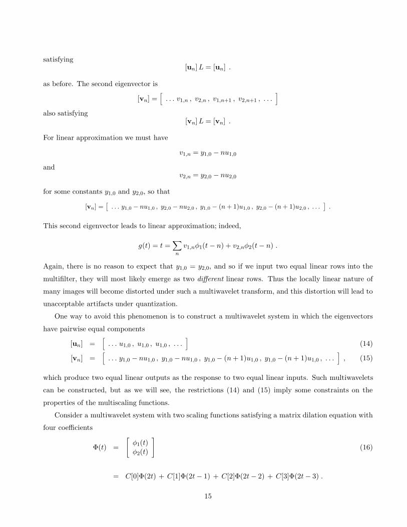
as before. The second eigenvector is
[vn] =[
. . . v1,n , v2,n , v1,n+1 , v2,n+1 , . . .]
also satisfying[vn]L = [vn] .
For linear approximation we must have
v1,n = y1,0 − nu1,0
andv2,n = y2,0 − nu2,0
for some constants y1,0 and y2,0, so that
[vn] =[
. . . y1,0 − nu1,0 , y2,0 − nu2,0 , y1,0 − (n + 1)u1,0 , y2,0 − (n + 1)u2,0 , . . .]
.
This second eigenvector leads to linear approximation; indeed,
g(t) = t =∑
n
v1,nφ1(t − n) + v2,nφ2(t − n) .
Again, there is no reason to expect that y1,0 = y2,0, and so if we input two equal linear rows into the
multifilter, they will most likely emerge as two different linear rows. Thus the locally linear nature of
many images will become distorted under such a multiwavelet transform, and this distortion will lead to
unacceptable artifacts under quantization.
One way to avoid this phenomenon is to construct a multiwavelet system in which the eigenvectors
have pairwise equal components
[un] =[
. . . u1,0 , u1,0 , u1,0 , . . .]
(14)
[vn] =[
. . . y1,0 − nu1,0 , y1,0 − nu1,0 , y1,0 − (n + 1)u1,0 , y1,0 − (n + 1)u1,0 , . . .]
, (15)
which produce two equal linear outputs as the response to two equal linear inputs. Such multiwavelets
can be constructed, but as we will see, the restrictions (14) and (15) imply some constraints on the
properties of the multiscaling functions.
Consider a multiwavelet system with two scaling functions satisfying a matrix dilation equation with
four coefficients
Φ(t) =
[
φ1(t)
φ2(t)
]
(16)
= C[0]Φ(2t) + C[1]Φ(2t − 1) + C[2]Φ(2t − 2) + C[3]Φ(2t − 3) .
15
It is proven in [20] that the vectors u = [u1,0 u2,0] , y = [y1,0 y2,0] must satisfy the following system
of equations:u (C[0] + C[2]) = u
u (C[1] + C[3]) = u
yC[1] + (u + y)C[3] = 12y
yC[0] + (u + y)C[2] = 12(u + y) .
(17)
We want
u1,0 = u2,0 = u0 , (18)
and
y1,0 = y2,0 = y0 , (19)
i.e., y = (y0/u0) u. From the dilation equation (16) and the approximation constraints (17), it follows
that u is a mutual eigenvector of all four matrices C[k]:
u C[k] = c′ku, k = 0, 1, 2, 3 . (20)
Consider now a scalar function φ(t)
φ(t) =1
u0u Φ(t) = φ1(t) + φ2(t).
According to (16) and (20), φ(t) satisfies the scalar dilation equation
φ(t) = c′0φ(2t) + c′1φ(2t − 1) + c′2φ(2t − 2) + c′3φ(2t − 3).
The only solution to this equation with orthogonal translates and second order of approximation is
Daubechies’ D4 scaling function [10]. Thus any orthogonal pair {φ1 , φ2} which has second order of
approximation, satisfies the dilation equation (16), and the eigenvector constraints (18) — (19) must
sum to D4:
φ1(t) + φ2(t) = D4(t).
We call such pairs “constrained” multiscaling functions. There are infinitely many constrained orthogonal
solutions of (20). Plots of two of them are shown in Figures 8 and 9. The ideas similar to those under-
lying “constrained” multiwavelets were used in [25] in order to construct different types of “balanced”
multiwavelets.
The implementation of constrained multiwavelets for the two-dimensional wavelet transform is straight-
forward. In each step of Mallat’s algorithm [26], one first processes pairs of rows and then pairs of columns.
Because locally constant and linear data are passed through to the lowpass ouputs of a constrained mul-
tifilter, the performance of these constrained multiwavelets in image compression is much better than
that of the “non-constrained” GHM pair, when applied by using two adjacent rows as the input. This is
confirmed by the experiments reported in the next section, as shown in Tables 4 and 5.
16

0.5 1 1.5 2 2.5 3
-0.2
-0.1
0.1
0.2
0.5 1 1.5 2 2.5 3
-0.2
-0.1
0.1
0.2
Figure 8: Constrained Pair 1.
0.5 1 1.5 2 2.5 3
-0.2
-0.1
0.1
0.2
0.5 1 1.5 2 2.5 3
-0.1
0.1
0.2
0.3
Figure 9: Constrained Pair 2.
6 Signal processing applications of multiwavelets
In this section we are going to compare the numerical performance of GHM and constrained multiwavelets
with Daubechies D4 scalar wavelets. We perform these comparisons in two standard wavelet applications:
signal denoising and data compression. We first develop these applications for one-dimensional signals,
then extend them to images. D4 wavelets were chosen because they have two vanishing moments, are
orthogonal and have four coefficients in the dilation equation — exactly like the GHM and constrained
pairs. For the application to image coding, we also add the (3,5)-tap scalar wavelet of LeGall and
Tabatabai to the mix. It has second-order approximation as well as linear-phase symmetry, at the cost
of biorthogonality instead of orthogonality.
6.1 Denoising by thresholding
Suppose that a signal of interest f has been corrupted by noise, so that we observe a signal g:
g[n] = f [n] + σz[n], n = 0 , 1, . . . , N − 1 .
where z[n] is unit-variance, zero-mean Gaussian white noise. What is a robust method for recovering f
from the samples g[n] as best as possible? Donoho and Johnstone [11, 12] have proposed a solution via
wavelet shrinkage or thresholding in the wavelet domain. Wavelet shrinkage works as follows:
17

1. Apply J steps of the cascade algorithm to get the N −N/2J wavelet coefficients and N/2J scaling
coefficients corresponding to g[n].
2. Choose a threshold tN = σ√
2 log(N) and apply thresholding to the wavelet coefficients (leave the
scaling coefficients alone).
3. Invert the cascade algorithm to get the denoised signal f [n].
We use hard thresholding when a wavelet coefficient wjk stays unchanged if wjk ≥ tN and is set to zero
if wjk < tN . Donoho and Johnstone’s algorithm offers the advantages of smoothness and adaptation.
Wavelet shrinkage is smooth in the sense that the denoised estimate f has a very high probability of being
as smooth as the original signal f , in a variety of smoothness spaces (Sobolev, Holder, etc.). Wavelet
shrinkage also achieves near-minimax mean-square-error among possible denoisings of f , measured over
a wide range of smoothness classes. In these numerical senses, wavelet shrinkage is superior to other
smoothing and denoising algorithms. Heuristically, wavelet shrinkage has the advantage of not adding
“bumps” or false oscillations in the process of removing noise, because of the local and smoothness-
preserving nature of the wavelet transform. Wavelet shrinkage has been successfully applied to SAR
imagery as a method for clutter removal [28]. It is natural to attempt to use multiwavelets as the
transform for a wavelet shrinkage approach to denoising, and compare the results with scalar wavelet
shrinkage.
We implemented Donoho’s wavelet shrinkage algorithm and compared the performance of the D4
scalar wavelet transform with oversampled and critically sampled multiwavelet schemes. The length of
the test signal was N = 512 samples. We chose J = 4 for the critically sampled multiwavelet method
and J = 5 for oversampled multiwavelet method and D4 scalar method (thus 16 scaling coefficients were
left untouched). In the oversampled scheme, the first row is multiplied by√
2, to better match the first
eigenvector of the GHM system. The critically sampled scheme uses the formulas (9) to obtain two
input rows v1,n, v2,n from a single row of data. After reconstruction the two output rows v1,n, v2,n are
deapproximated using (8), to yield the output signal f [n]. Boundaries are handled by symmetric data
extension for the critically sampled (approximation/deapproximation) and oversampled schemes, and by
circular periodization for D4.
Results of a typical experiment are shown in Table 1 and Figure 10. In all experiments both types
of GHM filter banks performed better than D4. The “repeated row” usually gave better results than
“approximation” preprocessing. This is not surprising, because “repeated row” is an oversampled data
representation, and it is well known that oversampled representations are useful for feature extraction.
Detailed discussion of denoising via multiwavelet thresholding, different estimates of the threshold
and more results of numerical tests can be found in [8, 40].
18

Original signal, 512 samples. Range of amplitude [−3, 10]
Noisy signal. Noise level σ = 0.3
Signal reconstructed using GHM with “approximation”.
Signal reconstructed using GHM with “repeated row”.
Signal reconstructed using D4.
Figure 10: Denoising via wavelet-shrinkage
19

GHM with GHM with
Noise approximation repeated row D4
mean absolute error 0.243 0.127 0.123 0.153
root mean square error 0.300 0.196 0.177 0.227
Table 1: Denoising via wavelet soft thresholding
6.2 Thresholding for compression of one-dimensional signals
We also performed a model compression experiment, using the same one-dimensional signal as in the
denoising experiments. We applied seven iterations of the cascade algorithm on this 512-point signal to
get the wavelet coefficients λk, using the same three types of wavelet and multiwavelet filter banks. For a
fair comparison, we retained the same number of the largest coefficients for each transform, then inverted
the cascade algorithm to reconstruct the signal. The results are shown in Table 2 and Figure 11.
GHM with “appr.” GHM with “rep. row” D4
recon with 50 largest coeffs.
`1 error 0.1298 0.1597 0.1807
`2 (mean square) error 0.0448 0.0517 0.0815
`∞ (maximum) error 1.5709 1.0667 1.4923
recon with 75 largest coeffs.
`1 error 0.0601 0.0650 0.0890
`2 (mean square) error 0.0091 0.0107 0.0200
`∞ (maximum) error 0.7959 0.9731 0.7301
recon with 100 largest coeffs.
`1 error 0.0320 0.0389 0.0466
`2 (mean square) error 0.0029 0.0030 0.0049
`∞ (maximum) error 0.2821 0.2309 0.2867
Table 2: One-dimensional compression by retention of largest coefficients.
For a given number of retained coefficients, the multiwavelet transforms lead to smaller `1 (mean
absolute) and `2 (root mean square) errors than the D4 scalar wavelet transform, and comparable `∞
(maximum) errors. GHM with “approximation” is slightly superior to GHM with “repeated row”. The
results of this experiment led us to try using the GHM multiwavelet with “approximation” for two-
dimensional image compression (with a true quantizer and coder), as discussed in Section 6.4 below.
20

Original signal, 512 samples. Range of amplitude [−3, 10]
Reconstruction from 75 largest coeffs of GHM with “approximation”.
Reconstruction from 75 largest coeffs of GHM with “repeated row”.
Reconstruction from 75 largest coeffs of D4 transform.
Figure 11: One-D signal compression via retention of large coefficients.
21

6.3 Denoising of images
Given the success of the multiwavelets in denoising of the model one-dimensional signal, we applied
multiwavelet denoising to imagery. We added white Gaussian noise with variance σ = 25 to 512 by
512 Lena image, and applied three wavelet transforms for denoising by wavelet shrinkage: GHM with
approximation preprocessing, GHM with repeated row preprocessing, and the Daubechies 4-tap scalar
wavelet. As in the 1-D case, the depth of the cascade was chosen to be J = 4 for GHM with approximation
and J = 5 for GHM with repeated row and D4. The experimental results are shown in Table 3 and in
Figure 12. Multiwavelet schemes were superior to D4 both numerically and subjectively. According to
our expectations GHM with repeated row preprocessing slightly outperformed GHM with approximation-
based preporcessing in terms of mean square error. Visually, multiwavelet schemes seemed to preserve
the edges better (especially GHM with repeated row) and reduce the Cartesian artifacts present in the
scalar wavelet shrinkage. This can be seen, for example, in the facial features (eyes, nose, lips) of the
Lena images shown in Figure 12.
GHM with GHM withNoise approximation repeated row D4
`1 error 19.93 7.11 7.90 8.71
`2 error 24.99 10.56 10.53 12.79
Table 3: Denoising of Lena image via wavelet shrinkage.
6.4 Transform-based image coding
One of the most successful applications of the wavelet transform is image compression. A transform-
based coder operates by transforming the data to remove redundancy, then quantizing the transform
coefficients (a lossy step), and finally entropy coding the quantizer output. Because of their energy
compaction properties and correspondence with the human visual system, wavelet representations have
produced superior objective and subjective results in image compression [26, 47, 2, 5]. Since a wavelet
basis consists of functions with short support for high frequencies and long support for low frequencies,
large smooth areas of an image may be represented with very few bits, and detail added where it is
needed. Multiwavelet decompositions offer all of these traditional advantages of wavelets, as well as the
combination of orthogonality, short support, and symmetry. The short support of multiwavelet filters
limits ringing artifacts due to subsequent quantization. Symmetry of the filter bank not only leads to
efficient boundary handling, it also preserves centers of mass, lessening the blurring of fine-scale features.
Orthogonality is useful because it means that rate-distortion optimal quantization strategies may be
employed in the transform domain and still lead to optimal time-domain quantization, at least when
error is measured in a mean-square sense. Thus it is natural to consider the use of multiwavelets in a
22

Lena image with Gaussian noise GHM with approximationMSE 24.99 multiwavelet denoising, MSE 10.56
Daubechies 4 scalar GHM repeated row
wavelet denoising, MSE 12.79 multiwavelet denoising, MSE 10.53
Figure 12: Multiwavelet denoising
23

transform-based image coder.
We employed a production image coder to compare the two-dimensional multiwavelet algorithms of
Section 5 with two scalar wavelets: the Daubechies 4-tap orthogonal wavelet and the (3,5)-tap symmetric
QMF of LeGall and Tabatabai. Five types of wavelet transform were used:
• (3,5)-tap scalar wavelet
• D4 scalar wavelet
• Approximation-based preprocessing with GHM multiwavelets
• Approximation-based preprocessing with Chui-Lian multiwavelets
• Adjacent rows input with the constrained pair #1 multiwavelet
• Adjacent rows input with the constrained pair #2 multiwavelet
Each of these wavelet transforms was followed by entropy-constrained scalar quantization and entropy
coding. We made the assumption that the histograms of subband (or wavelet transform subblock) coeffi-
cient values obeyed a Laplacian distribution [26], and designed a uniform scalar quantizer. The quantizer
optimized the bit allocation among the different subbands by using an operational rate-distortion ap-
proach (minimizing the functional D +λR) [33]. We then entropy-coded the resulting coefficient streams
using a combination of zero-run-length coding and adaptive Huffman coding, as in the FBI’s Wavelet
Scalar Quantization standard [14].
We applied these different wavelet image coders to the Lena (NITF6) image, as well as a geometric
test pattern, at a variety of compression ratios. The results are shown in Tables 4 and 5, and in Figures
13 and 14. On Lena, the Chui-Lian multiwavelet outperformed both the D4 and (3,5) scalar wavelets,
while the GHM multiwavelet was comparable with D4 and outperformed (3,5) at compression ratios of
32:1 and 64:1. The images in Figure 13 show that both the approximation-based multiwavelet schemes
produce fewer Cartesian artifacts than the scalar wavelet, and the Chui-Lian multiwavelet preserves
more detail (e.g. the eyelashes). The adjacent-row method did not work well on Lena. However, the
adjacent-row method did do well on the geometric test pattern image (Figure 14) with the constrained
pair #1 “CP-1” outperforming D4 (and GHM with approximation) at the 8:1 compression ratio. When
using the repeated row algorithm, the constrained pairs significantly outperformed the GHM symmetric
multiwavelet, demonstrating the importance of the eigenvector constraints (14) - (15). A close look at
the details of the compressed/decompressed test patterns shows that the CP-1 compression “rang” over a
shorter distance than the D4 compression. While the (3,5)-tap scalar wavelet produced minimal ringing,
24

it significantly degraded the checkerboard pattern. The Chui-Lian multiwavelet did the best, yielding a
lossless (!) compression at 8:1 and beating all contenders at all compression ratios.
These preliminary results suggest that multiwavelets are worthy of further investigation as a technique
for image compression. Issues to address include the design of multiwavelets with symmetry and higher
order of approximation than the GHM system, the role of eigenvector constraints, and also further
exploration of regularity for multiwavelets [42]. One might also apply zerotree-coding methods [32] in a
multiwavelet context. Other interesting results on implementation of multiwavelets for image compression
can be found in [7].
Compression Ratio 8:1 16:1 32:1 64:1
pSNR pSNR pSNR pSNR
(3,5)-tap scalar QMF 37.6 33.1 30.2 27.1
Daubechies 4 38.0 34.6 31.3 28.41
GHM with appr./deappr. 37.5 34.0 31.1 28.5
Chui-Lian with appr./deappr. 38.3 34.7 31.5 28.4
constrained pair #1 35.3 31.1 27.9 25.5
constrained pair #2 34.4 30.4 27.3 24.9
Table 4: Peak SNRs for compression of Lena.
Compression Ratio 8:1 16:1 32:1 64:1
pSNR pSNR pSNR pSNR
(3,5)-tap scalar QMF 63.8 36.2 23.1 16.5
Daubechies 4 78.2 44.9 31.5 21.8
GHM with appr./deappr. 56.7 35.7 27.2 22.2
Chui-Lian with appr./deappr. ∞ 57.3 37.0 27.3
constrained pair 1 91.2 41.6 29.2 21.8
constrained pair 2 53.6 34.6 24.8 21.1
Table 5: Peak SNRs for compression of geometric test pattern.
25

Original Lena image (3,5)-tap scalar wavelet32:1 compression, pSNR 30.2
Daubechies 4 Constrained Pair #1
32:1 compression, pSNR 31.3 32:1 compression, pSNR 27.9
GHM with approximation Chui-Lian with approximation
32:1 compression, pSNR 31.1 32:1 compression, pSNR 31.5
Figure 13: Wavelet and multiwavelet compression of Lena image.
26

Original geometric pattern Detail of original pattern
Daubechies 4 scalar wavelet Biorthogonal 3-5 scalarcompression (32:1, pSNR 31.52) compression (32:1, pSNR 23.05)
Chui-Lian with approximation Constrained pair #1 adjacent rowmultiwavelet compression multiwavelet compression
(32:1, pSNR 37.04) (32:1, pSNR 29.16)
Figure 14: Wavelet and multiwavelet compression of geometric pattern.
27

7 Conclusions
After reviewing the recent notion of multiwavelets (matrix-valued wavelet systems), we have examined
the use of multiwavelets in a filter bank setting for discrete-time signal processing. Multiwavelets offer the
advantages of combining symmetry, orthogonality, and short support, properties not mutually achievable
with scalar 2-band wavelet systems. However, multiwavelets differ from scalar wavelet systems in requir-
ing two or more input streams to the multiwavelet filter bank. We described two methods (repeated row
and approximation/deapproximation) for obtaining such a vector input stream from a one-dimensional
signal. We developed the theory of symmetric extension for multiwavelet filter banks, which matches
nicely with approximation-based preprocessing. Moving on to two-dimensional signal processing, we
described an additional algorithm for multiwavelet filtering (two rows at a time), and developed a new
family of multiwavelets (the constrained pairs) that is well-suited to this two-row-at-a-time filtering.
We then applied this arsenal of techniques to two basic signal processing problems, denoising via
thresholding (wavelet shrinkage), and data compression. After developing the approach via model prob-
lems in one dimension, we applied the various new multiwavelet approaches to the processing of images,
frequently obtaining performance superior to the comparable scalar wavelet transform. These results
suggest that further work in the design and application of multiwavelets to signal and image processing
is well warranted.
Acknowledgments: We would like to thank Scott Hills for help programming the image com-
pressions, and Stephane Mallat for useful discussions.
References
[1] B. Alpert, “A class of bases in L2 for the sparse representation of integral operators,” SIAM J. Math. Analysis,
vol. 24, 1993.
[2] M. Antonini, M. Barlaud, P. Mathieu, and I. Daubechies, “Image coding using the wavelet transform,” IEEE
Trans. on Image Processing, vol. 1, pp. 205-220, 1992.
[3] R. H. Bamberger, S. L. Eddins, and V. Nuri, “Generalized symmetric extension for size-limited multiratefilter banks,” IEEE Trans. on Image Proc., vol. 3, pp. 82-86, 1994.
[4] C. Brislawn, “Classification of symmetric wavelet transforms,” Los Alamos Technical Report, 1993.
[5] B. V. Brower, “Low-bit-rate image compression evaluations,” Proc. SPIE, Orlando, FL, April 4-9, 1994.
[6] C. K. Chui and J. A. Lian “A Study of Orthonormal Multiwavelets,” J. Appl. Numer. Math., vol. 20, pp.272-298, 1996.
[7] M. Cotronei, L. B. Montefusco, and L. Puccio, “Multiwavelet analysis and signal processing,” IEEE Trans.
on Circuits and Systems II, to appear.
28

[8] T. Downie and B. Silverman, “The discrete multiple wavelet transform and thresholding methods,” IEEE
Trans. on Signal Proc., to appear.
[9] W. Dahmen, B. Han, R.-Q. Jia, and A. Kunoth, “Biorthogonal multiwavelets on the interval: cubic Hermitesplines,” preprint, 1998.
[10] I. Daubechies, Ten Lectures on Wavelets, Philadelphia: SIAM, 1992.
[11] D. Donoho, “De-noising by soft-thresholding,” IEEE Trans. Inf. Theory, vol. 41, pp. 613-627, 1995.
[12] D. L. Donoho and I. M. Johnstone, “Ideal spatial adaptation via wavelet shrinkage,” Biometrika, vol. 81, pp.425-455, 1994.
[13] G. Donovan, J. Geronimo, and D. Hardin, “Intertwining multiresolution analyses and the construction ofpiecewise polynomial wavelets,” SIAM J. Math. Anal., vol. 27, pp. 1791-1815, 1996.
[14] Fed. Bureau of Investig., WSQ Gray-Scale Fingerprint Image Compression Specification, drafted by T. Hop-per, C. Brislawn, and J. Bradley, IAFIS-IC-0110-v2, Feb. 1993.
[15] V. M. Gadre and R. K. Patney, “Vector multirate filtering and matrix filter banks,” Proc. IEEE ISCAS, SanDiego, 1992.
[16] J. Geronimo, D. Hardin, and P. R. Massopust, “Fractal functions and wavelet expansions based on severalfunctions,” J. Approx. Theory, vol. 78, pp. 373-401, 1994.
[17] R. A. Gopinath, J. E. Odegard, and C. S. Burrus, “Optimal wavelet representation of signals and the waveletsampling theorem,” IEEE Trans. on Circ. and Sys. II, vol. 41, pp. 262-277, 1994.
[18] D. Hardin and J. Marasovich, “Biorthogonal multiwavelets on [-1,1],” preprint, 1997.
[19] D. Hardin and D. Roach, “Multiwavelet prefilters I: orthogonal prefilters preserving approximation orderp ≤ 2,” preprint, 1997.
[20] C. Heil, G. Strang, and V. Strela, Approximation by translates of refinable functions,” Numerische Mathe-
matik, vol. 73, pp. 75-94, 1996.
[21] P. Heller, V. Strela, G. Strang, P. Topiwala, C. Heil, and L. Hills, “Multiwavelet filter banks for data com-pression,” Proc. IEEE ISCAS, Seattle, WA, May 1995.
[22] Q. Jiang, “Parametrization of M -channel orthogonal multifilter banks,” preprint, 1997.
[23] H. Kiya, K. Nishikawa, and M. Iwahashi, “A Development of symmetric extension method for subband imagecoding,” IEEE Trans. on Image Proc., vol. 3, pp. 78-81, 1994.
[24] W. Lawton, S. L. Lee, and Z. Shen, “An algorithm for matrix extension and wavelet construction,” Mathe-
matics of Computation, Math. Comp., vol. 65, pp. 723-737, 1996.
[25] J. Lebrun and M. Vetterli, “Balanced multiwavelets: theory and design,” Proc. IEEE ICASSP, Munich, 1997.
[26] S. Mallat, “A theory for multiresolution signal decomposition: the wavelet representation,” IEEE Trans.
PAMI, vol. 11, pp. 674-693, 1989.
[27] J. Miller and C. Li, “Adaptive miltiwavelet initialization,” preprint 1997.
[28] J. Odegard, M. Lang, H. Guo, R. Gopinath, and C. Burrus, “Nonlinear wavelet processing for enhancementof images,” submitted to IEEE SP Letters, 1994.
[29] G. Plonka, “Approximation order provided by refinable function vectors,” Const. Approx., vol 13, pp. 221-244,1997.
29

[30] G. Plonka, “Generalized spline wavelets,” Constr. Approx., vol. 12, pp. 127-155, 1996.
[31] G. Plonka and V. Strela, “Construction of multi-scaling functions with approximation and symmetry,” SIAM
J. Math. Anal., to appear.
[32] J. M. Shapiro, “Embedded image coding using zerotrees of wavelet coefficients,” IEEE Trans. on SP, vol. 41,pp. 3445-3662, 1993.
[33] Y. Shoham and A. Gersho, “Efficient bit allocation for an arbitrary set of quantizers,” IEEE Trans. ASSP,vol. 36, pp. 1445-1453, 1988.
[34] M. J. T. Smith and S. Eddins, “Analysis-synthesis techniques for subband image coding,” IEEE Trans. ASSP,
vol. 38, pp. 1446-1456, 1990.
[35] G. Strang and T. Nguyen, Wavelets and Filter Banks, Wellesley, MA: Wellesley-Cambridge Press, 1995.
[36] G. Strang and V. Strela, “Short wavelets and matrix dilation equations,” IEEE Trans. on SP, vol. 43, pp.108-115, 1995.
[37] G. Strang and V. Strela, “Orthogonal multiwavelets with vanishing moments,” J. Optical Eng., vol. 33 , pp.2104-2107, 1994.
[38] V. Strela, “A Note on Construction of Biorthogonal Multi-scaling Functions,” in Contemporary Mathematics,A. Aldoubi and E. B. Lin (eds.), AMS 1998.
[39] V. Strela and G. Strang, “Finite element multiwavelets,” Proc. NATO Conference, Maratea, Boston, MA:Kluwer, 1995.
[40] V. Strela and A. T. Walden, “Signal and image denoising via wavelet thresholding: orthogonal and biorthog-onal, scalar and multiple wavelet transforms,” Statistics Section Technical Report TR-98-01, Dep. of Math.,
Imperial College, London, 1998.
[41] G. Uytterhoeven, Multiwavelets for image compression, Masters thesis, Katholieke Universiteit Leuven, May,1994.
[42] M. Vetterli and G. Strang, “Time-varying filter banks and multiwavelets,” Sixth IEEE DSP Workshop,Yosemite, 1994.
[43] M. Vrhel and A. Aldroubi, “Projection based pre-filtering for multiwavelet transforms,” preprint, 1997.
[44] X.-G. Xia, “ A new prefilter design for discrete multiwavelet transforms,” preprint, 1996.
[45] X.-G. Xia, J. Geronimo, D. Hardin, and B. Suter, “Computations of multiwavelet transforms,” Proc. SPIE
2569, San Diego, CA, July 1995.
[46] X.-G. Xia, J. Geronimo, D. Hardin, and B. Suter, “Design of prefilters for discrete multiwavelet transforms,”IEEE Trans. on Signal Proc., vol. 44, pp25-35, 1996.
[47] W. Zettler, J. Huffman, and D. Linden. “The application of compactly supported wavelets to image compres-sion,” Proc. SPIE 1244, pp. 150-160, 1990.
30