Embed Size (px)
Citation preview

The Aggregate Impact of Antidumping Policies
April 2014 (Preliminary)
Kim J. Ruhl*New York University Stern School of Business
ABSTRACT—————————————————————————————————————Multilateral trade agreements, such as the GATT/WTO, have severely restricted the ability ofcountries to raise tariffs on imports. One of the few tools still available to policy makers under theWTO rules is antidumping law — and antidumping investigations have become a major imped-iment to free trade. The United States has initiated more than 1200 antidumping investigationssince 1980; globally, more than 200 antidumping investigations are initiated per year.
The existing literature on the impact of antidumping policy has primarily focused on industrylevel models and the strategic interactions between firms. In this paper I develop a tractable modelof antidumping policy and embed it into a general equilibrium model with heterogeneous firmsand monopolistic competition. The model of antidumping policy embodies two key features ofthe existing law: firms charging “low” prices are (i) more likely to be accused of dumping and (ii)face larger antidumping duties.
In the calibrated model, the existing U.S. antidumping policy has an aggregate impact equiv-alent to a 6 percent tariff that is uniformly applied to all firms. The welfare costs of antidumpingpolicy come, not only from the higher prices charged by firms subject to antidumping duties, butalso from the higher prices that all exporting firms optimally charge in order to minimize the prob-ability of being accused of dumping.———————————————————————————————————————————
*I would like to thank John Asker, Eric Bond, and Mike Waugh for helpful discussions. This work was undertaken withthe support of the National Science Foundation under grant SES-0536970.

1 Introduction
Multilateral trade agreements, such as the General Agreement on Trade and Tariffs/World Trade
Organization (GATT/WTO), have severely restricted the ability of countries to raise tariffs on
imports. One of the few tools still available to policy makers under the WTO rules is antidump-
ing law — and antidumping investigations have become a major impediment to free trade. The
United States has initiated more than 1200 antidumping investigations since 1980; globally, more
than 200 antidumping investigations are initiated per year. U.S. President Barack Obama even
made it a central point of his 2012 State of the Union Address, saying:
We’ve brought trade cases against China at nearly twice the rate as the last administra-
tion — and it’s made a difference. But we need to do more. Tonight, I’m announcing
the creation of a Trade Enforcement Unit that will be charged with investigating unfair
trading practices in countries like China. (Obama, 2012)
In this paper I build a model of antidumping policy and embed it into a general equilibrium
trade model to determine the aggregate impact of antidumping policy on trade flows, prices, and
welfare. A major obstacle in developing an aggregate model of antidumping is the complicated
nature of antidumping law. A domestic firm must show that an imported good is being priced at
“less than fair value,” and that the dumped imports have caused, or could cause, material injury
to the domestic industry. In particular, the difficulty in determining at what price a foreign firm
should be selling its good injects substantial arbitrariness into antidumping investigations.
To generate a tractable model of antidumping policy that preserves the main characteristics
of the observed framework, I take a probabilistic approach. I model an antidumping policy as a
function that takes as arguments the price charged by a foreign firm and a reference price, and
assigns to the firm a probability that it will be penalized for dumping. In general, the lower
is the price charged by the foreign firm, the higher is the probability the firm will have to pay
antidumping duties. To be consistent with current policy, the size of the antidumping duty is also
a function of the price charged by the foreign firm and the reference price: the lower is the price
charged by the foreign firm, the larger is the antidumping tariff.
2

The model is calibrated to match the United States and a symmetric trading partner. The cali-
bration targets the usual statistics of interest in the trade literature as well as characteristics of the
observed antidumping cases initiated by the United States. I find that the calibrated antidumping
policy has the same impact on trade flows as a uniformly applied tariff of 6 percent—about the
size of the average current U.S. tariff. Antidumping policy distorts imports in two ways. First,
consumers pay higher prices for goods from firms that are being punished for dumping. Sec-
ond, firms that are not being punished for dumping charge a higher price than they would in
the absence of antidumping policy because the higher price reduces the probability that they are
punished for dumping in the future. On average, tradable good firms who are not paying an-
tidumping duties choose markups that are 2 percentage points higher than in a model without
antidumping policy.
Combining heterogeneous firms and an antidumping policy that targets low-priced imports
generates a friction that correlates with firm productivity. Since antidumping duties are larger for,
and more likely to be imposed on, more productive firms, antidumping policy generates a larger
friction for more productive firms. This aspect of the model is an example of the kind of size-
dependent policy distortions studied in Restuccia and Rogerson (2008) and Guner, Ventura and
Yi (2008). Analogous to their closed economy findings, I find that the size dependence induced
by antidumping policy generates stronger welfare effects than a simple tariff that is uniformly
applied to all importers.
The differential welfare effects are large when I incorporate low-cost trading partners into the
model. As developing countries—most notably China and India—have become important ex-
porters, antidumping cases against these countries have exploded. China, alone, accounts for
more than 20 percent of all antidumping investigations initiated worldwide since 1995. I model
the inclusion of new trade partners as a 50 percent increase in the size of the foreign country in
both a model with antidumping duties and in a model with only uniform tariffs. In this experi-
ment, wages in the foreign country fall by 7 percent in both models, but import prices behave in
different ways. In the model without antidumping policy, the drop in production costs is com-
pletely passed through to the home country: markups are constant in this model. In the model
with antidumping, firms—concerned that lowering their prices will generate large antidumping
duties—increase their markups, passing-through only a portion of the decrease in marginal costs.
3
The differential pricing behavior shows up in welfare: in the model with antidumping policy, wel-
fare increases by 1.5 percent, but in the model without antidumping policy welfare increases by
2.3 percent.
Proponents of antidumping laws usually appeal to some form of predatory pricing: a foreign
firm will dump cheap goods into the domestic market to drive domestic firms out of the market,
and then, once the foreign firm has gained market power, it increases its price and earns economic
rents. In this paper, I abstract from predatory pricing: firms are monopolistic competitors with
no predatory incentive. This eliminates any positive impact that antidumping law could have, so
the finding here should be considered an upper bound to the gain from eliminating antidumping
law. There is good reason, though, to be skeptical that observed antidumping duties have much
to do with predatory pricing. Among others, Moore (1992) and Hansen and Prusa (1996) find
that antidumping rulings have a strong political component, showing that various measures of
the political importance of an industry are significant predictors of antidumping rulings. Further,
Blonigen (2006) documents the ways that changes in the laws that govern the determination of
“fair value” have evolved over time, and finds that they have led to larger antidumping duties,
growing from an average of 10 percent in 1982 to 40 percent after 1990.
The previous theoretical literature on antidumping has largely focused on industry-level mod-
els and the strategic interaction between foreign firms, domestic firms, and regulators. Prusa
(1992) showed how domestic firms could strategically use antidumping investigations—even if a
duty is never levied—to restrict imports. Staiger and Wolak (1992) demonstrate that the threat of
antidumping can force foreign firms to behave in a less competitive manner. In this same vein,
the firms in the model developed below will react to the mere presence of antidumping policy by
increasing their markups to decrease the probability of being found guilty of dumping. This pa-
per builds on this literature by incorporating a model in which firms endogenously price to avoid
antidumping investigations into a general equilibrium structure.
Most closely related to this paper is the computable general equilibrium model in Gallaway,
Blonigen and Flynn (1999). Gallaway et al. (1999) construct a calibrated multisector model and
find that eliminating U.S. antidumping law would increase welfare on the order of 4 billion dol-
lars in 1993. The model developed in this paper is also concerned with the aggregate effects of
antidumping policy, but does so using a heterogeneous firm structure. By allowing for firm het-
4

erogeneity, I can study how the bias against productive firms—inherent in antidumping policy—
affects export decisions on both the extensive and intensive margins.
Lastly, it is worth noting that this paper is not asking if antidumping law is being correctly
implemented in an economic sense. The purpose of this paper is to model, in a parsimonious
way, several key features of antidumping law as it is currently written, and to study its effects in
a heterogeneous firm, general equilibrium model. For those interested, Stiglitz (1997) provides a
discussion on the economic justification—or lack thereof—for unfair trade law.
The paper is organized as follows. In section 2 I discuss antidumping law as it is administered
in the United States, and summarize key features of the law that motivate my implementation of
antidumping policy in the model. In sections 3-5 I develop a model of antidumping policy, embed
it into an otherwise standard trade model, and calibrate the model to match key facts about the
U.S. economy. In section 6 I show the impact of antidumping policy on trade and welfare, and
compute the tariff equivalent of the observed policy.
2 U.S. antidumping policy
Finger (1993) traces the origin of antidumping law to Canada, where it was used in 1904 to pro-
tect Canadian steel makers from low cost railroad rails from US Steel. From there, the United
States, Australia, and South Africa became early users of antidumping policy. Antidumping in-
vestigations have become more common as tariff binding in the GATT/WTO has made it difficult
to adjust tariffs. In this section I summarize some of the relevant features of U.S. antidumping
law to motivate the model of antidumping policy developed in section 3. Two characteristics are
particularly important: the degree to which an affirmative dumping finding is based on difficult
to measure “fair value” concepts, and the typical duration of an antidumping duty.
When a domestic firm (or more often, a coalition of firms) files an antidumping petition, two
conditions have to be met to trigger an antidumping duty. It must be found that the imports are
being sold at below “fair value,” and that these dumped imports have caused, or threaten to cause,
material damage to domestic industry. In the U.S., two agencies are responsible for antidumping
investigations. The Department of Commerce (DOC) is tasked with determining if the goods in
question are being sold at below fair value, and the International Trade Commission determines
if the imported goods have caused material injury to the domestic industry.
5
Determining the fair value price of an import can be complicated. Ideally, the DOC can ob-
serve the identical good being sold in the importing firm’s home market; if so, the home market
price is considered the fair value price.1 It is rarely the case, however, that the identical good exists
in the importer’s home country. Lacking an identical good for comparison, the DOC will compare
the average U.S. price to the average home market price of the “next most similar product.” (Lind-
sey and Ikenson, 2003) Finding a comparable product in the exporter’s home country creates an
arbitrariness in the dumping criteria. In addition, regardless of the pricing method, several price
adjustments are made before the final “fair value” is determined.
The DOC also has the administrative authority to declare a country to be a nonmarket economy,
meaning that prices in the country do not reflect the fair value of goods. The DOC applies a spe-
cial methodology to nonmarket economies: prices of goods in comparable countries are used to
construct the fair value price. Firms from nonmarket economies must also provide information
about the extent of government involvement in their operations. Most notably, the DOC has de-
clared China—the most frequent target of U.S. antidumping investigations—to be a nonmarket
economy.
The significant leeway in determining the fair value price, and the inherent political nature
of the system, motivate the key simplifying assumption in the model that follows: through no
fault of its own, a firm may be charged with dumping even if it is not engaging in anticompetitive
behavior. To capture the idea that low prices are necessary for both finding a firm guilty of dump-
ing and for finding injury, the antidumping policy in the model assigns each firm a probability of
facing an antidumping duty that is decreasing in the firm’s export price.
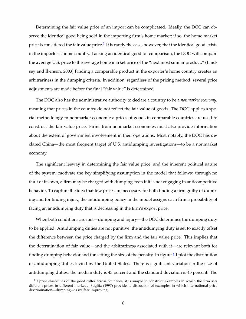
When both conditions are met—dumping and injury—the DOC determines the dumping duty
to be applied. Antidumping duties are not punitive; the antidumping duty is set to exactly offset
the difference between the price charged by the firm and the fair value price. This implies that
the determination of fair value—and the arbitrariness associated with it—are relevant both for
finding dumping behavior and for setting the size of the penalty. In figure 1 I plot the distribution
of antidumping duties levied by the United States. There is significant variation in the size of
antidumping duties: the median duty is 43 percent and the standard deviation is 45 percent. The
1If price elasticities of the good differ across countries, it is simple to construct examples in which the firm setsdifferent prices in different markets. Stiglitz (1997) provides a discussion of examples in which international pricediscrimination—dumping—is welfare improving.
6
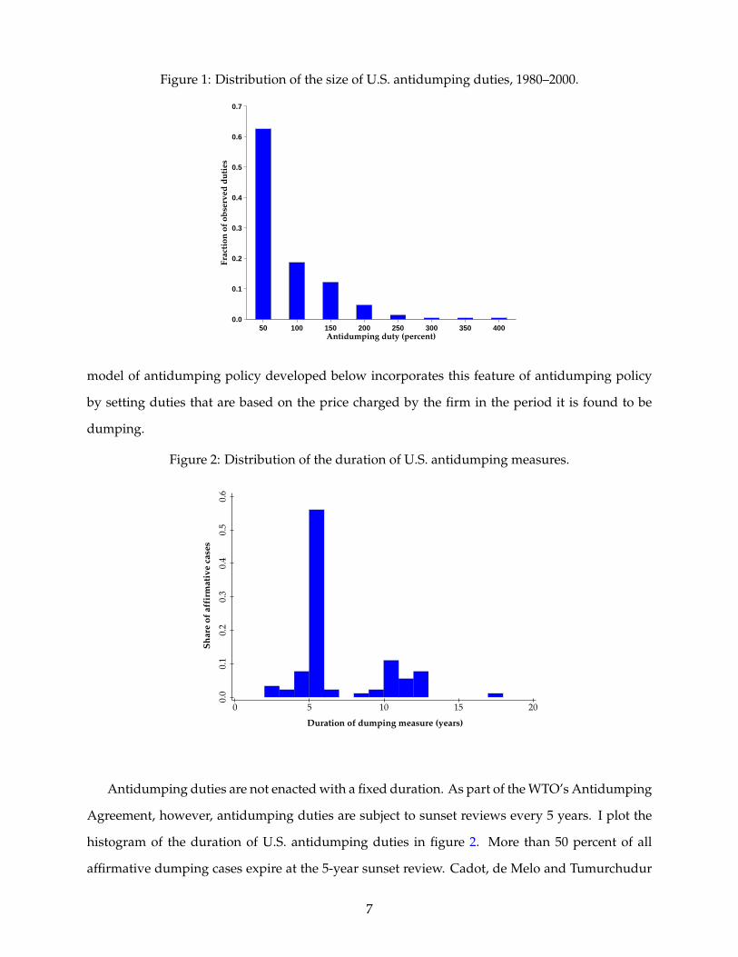
Figure 1: Distribution of the size of U.S. antidumping duties, 1980–2000.
50 100 150 200 250 300 350 4000.0
0.1
0.2
0.3
0.4
0.5
0.6
0.7
Antidumping duty (percent)
Fra
ctio
n o
f o
bse
rved
du
ties
model of antidumping policy developed below incorporates this feature of antidumping policy
by setting duties that are based on the price charged by the firm in the period it is found to be
dumping.
Figure 2: Distribution of the duration of U.S. antidumping measures.
0.0
0.1
0.2
0.3
0.4
0.5
0.6
Sh
are
of a
ffir
mat
ive
case
s
0 5 10 15 20
Duration of dumping measure (years)
Antidumping duties are not enacted with a fixed duration. As part of the WTO’s Antidumping
Agreement, however, antidumping duties are subject to sunset reviews every 5 years. I plot the
histogram of the duration of U.S. antidumping duties in figure 2. More than 50 percent of all
affirmative dumping cases expire at the 5-year sunset review. Cadot, de Melo and Tumurchudur
7

(2007) study a multi-country panel of dumping investigations and find that the median duration
of an antidumping duty in their larger sample is, indeed, 5 years, but they also find significant
variation: the coefficient of variation is 0.60 in their sample, with a maximum duration—found on
a U.S. levied duty—of almost 24 years. In the model of antidumping proposed in this paper, firms
exit an antidumping duty in a probabilistic way: this mechanism generates both long and short
lived antidumping duties.
3 Model
The world consists of two countries, home and foreign. Each country in populated by a stand-in
household who derives utility from consumption of a final good that is made up of tradable and
nontradable goods. Foreign country variables are marked with an asterisk.
3.1 Preferences
In this section I layout the decision problem for the household in the home country. The foreign
household’s problem is analogous. The household inelastically supplies labor, owns the capital
stock, and owns the firms that produce in the home country. Households choose consumption,
investment, and bond holdings to maximize utility,
∞∑t=1
βt log(Ct), (1)
subject to the household’s budget constraint and the law of motion for capital,
PT,t (CT,t + It) +Bt+1 ≤ wtL+ rktKt + (1 + rbt)Bt + Πt + Tt (2)
Kt+1 = (1 − δ)Kt + It, (3)
where Ct is consumption of the final good, It is investment, Kt is the capital stock, Πt is the
aggregate profit of domestic firms, and Tt is the lump-sum transfer of tariff and antidumping
revenues back to the household. Bt is the household’s holdings of one-period bonds.
3.2 Final good production
The final good, which is used for consumption and investment, is made up of a composite tradable
good and a composite nontradable good. The final good is produced with a constant returns to
8

scale production technology and sold in a perfectly competitive market, so the final good sector
can be modeled as a single representative firm. The final good firm’s maximization problem is
maxvF ,hF
PtYt−PT,thFt − PNT,tvFt (4)
s.t. Yt =(µTh
Fγt + vFγt
) 1γ, (5)
where vF is the quantity of the composite nontradable good and hF is the quantity of the compos-
ite tradable good used in the production of the final good. The elasticity of substitution between
tradable and nontradable goods in production is 1/(1−γ) and the parameter µT governs the share
of expenditure over tradable and nontradable goods in equilibrium. The price of the final good is
P−γ1−γt = µ
11−γT P
−γ1−γT,t + P
−γ1−γNT,t. (6)
3.3 Composite good firms
The nontradable and tradable composite goods are aggregates of differentiated varieties. The com-
posite goods are used to produce the final good and are used as intermediate inputs in the differ-
entiated varieties. The composite goods cannot be exported. The composite goods are produced
using constant returns to scale production technologies and are sold in perfectly competitive mar-
kets, so the composite good sectors can be modeled as each consisting of one representative firm.
The representative firm in tradable composite good sector chooses purchases of tradable dif-
ferentiated varieties yi from both domestic producers and foreign exporters to solve
maxyit
PT,tYT,t −∫i∈IT,t
pityit di−∫i∈IM,t
τxipityit di (7)
s.t. YT,t =
(∫i∈IT,t
yρit di+
∫i∈IM,t
yρit di
) 1ρ
(8)
where PT,t is the price of the composite tradable good and pit is the price of differentiated variety
i. Imported goods are subject to trade costs (a technological friction), tariffs (a policy friction),
and, potentially, antidumping duties (another policy friction). Tariffs are levied equally on all
imported goods, but antidumping duties are firm specific, which why the total trade cost, τxi > 1
is indexed by i. Note that the set of imported varieties available to the composite good firm, IM,t
9

is an equilibrium object, and will generally not include all of the varieties produced in the foreign
country. The elasticity of substitution between varieties in production is 1/(1 − ρ).
The representative firm in the nontradable composite good sector chooses purchases of non-
tradable differentiated varieties, yi from domestic producers to solve
max PNT,tYNT,t −∫i∈IN,t
pityit di (9)
s.t. YNT,t =
(∫i∈IN,t
yρit di
) 1ρ
(10)
where PT,t is the price of the composite tradable good and pit is the price of differentiated variety
i. The set of available nontradable differentiated goods is IN,t.
The solutions to the composite good problems generate demand functions for tradable and
nontradable varieties, yT (τxipit), and yNT (pit), and the price indices for the tradable and nontrad-
able composite goods,
PT,t =
(∫i∈IT,t
p−ρ1−ρit di+
∫i∈IM,t
(τitpit)−ρ1−ρ di
) 1−ρ−ρ
(11)
PNT,t =
(∫i∈INT,t
p−ρ1−ρit di
) 1−ρ−ρ
. (12)
3.4 Antidumping policy
Before laying out the differentiated good firm’s problem, I need to specify a model of antidumping
policy. As discussed in section 2, antidumping investigations are complicated affairs that center
around meeting two conditions: (i) the foreign firm is pricing below fair value and (ii) the dumped
imports have caused harm to the domestic industry. Given the various ways in which fair value
can be constructed, there exists an arbitrariness in determining whether a firm is dumping goods
into the domestic market. To incorporate these features in a tractable way, I model antidumping
policy as a probabilistic process. The lower a firm sets its price, the more likely it is to be charged
with dumping.
Specifically, a foreign firm who prices below the fair value price, p, may be charged with dump-
ing. The probability of being subject to an antidumping duty in the next period is made up of two
10

components. The first component is conditional on the price charged by the firm this period, p,
relative to the fair value price. The component is g(p, p), where g′(p, p) < 0 if p < p. It is through
this component that the firm can influence its probability of being punished: the higher the firm
sets its price, the lower is the probability of being punished.
The second component of the antidumping probability function is a small probability, λ, that
the firm is punished, regardless of the price it is charging. This “bad luck” component is meant
to capture the idea that antidumping investigations tend to cast a wide net that sometimes pick
up firms that are pricing close to the fair value price. These firms end up being charged small
antidumping duties, and this second component will allow the model to generate these small
duties. The probability of being punished for antidumping, conditional on the price a firm is
charging is
f(p, p) =
λ+ (1 − λ)g(p, p) if p < p
0 if p ≥ p(13)
This specification implies that a firm will never be charged with dumping if its price is equal to
or above fair value. Implicit in this definition is the assumption that the fair value price is the same
for all firms. This implies that more productive firms—who would like to charge lower prices—
will be at a greater risk for being charged with antidumping duties compared to low productivity
firms.
If a firm is charged with dumping, it pays an ad valorem duty of τAD(p) > 1 on its exports that
is based on the price it set when found guilty of dumping, denoted p. In the U.S. antidumping
code, the antidumping duty is such that the firm’s price, inclusive of the duty, is equal to the fair
value price. Consistent with this practice, the antidumping duty is
τAD(p) = 1 +p− p
p, (14)
Once a firm is convicted of dumping, it faces an exogenous probability of exiting the penalty
phase, denoted by θ.
11

3.5 Differentiated good firms
This section describes the firms in the home country. The foreign country has an analogous market
structure. A unit mass of potential tradeable good firms and a unit mass of potential nontradable
good firms exists each period. Both tradable and nontradable good firms use labor, capital, and
tradable and nontradable composite goods to produce differentiated varieties according to
yit =ϕi(kαitl
1−αit
)ωvωNit h
ωTit (15)
1 =ω + ωT + ωNT
where ϕ is the marginal productivity of a firm producing variety i. The productivity of potential
firms is distributed according to the probability density function g(ϕ). Firms are monopolistic
competitors who understand that they face the downward sloping demand derived in the previ-
ous section. If a tradeable good firm wishes to sell to the domestic market, it incurs a fixed cost of
κd units of labor to do so. For a tradable good firm, the profit from selling domestically is
πd(pit) = pityT,t(pit) − yT,t(pit) (pit −mcit) − wtκd (16)
mcit =1
ϕi
(rtα
)αω ( wt1 − α
)(1−α)ω (PNT,tωNT
)ωNT (PT,tωT
)ωT. (17)
If the tradeable good firm wishes to export to the foreign market, it incurs a fixed cost of κx units
of labor. In the export market, the firm pays an ad valorem cost τxi > 1. This cost embodies both
non-antidumping tariffs and transportation costs. Export profits of tradable good firms are
πx(pit, τx) = pity∗T,t (τxpit) − y∗T,t (τxpit) (pit −mcit) − wtκx. (18)
Denote the pre-tariff price as pit; the consumer pays τxipit. Since the production function has
constant returns to scale, decisions regarding production for the domestic market do not affect the
profit from exporting, and vice versa. This implies that the profit maximization problem of the
firm can be solved market-by-market.
The nontradable sector firms face the same fixed cost of operation, κd, but only earn profits
12

from selling domestically,
πn(pit) = pityNT,t(pit) −yNT,t(pit)wt
ϕit− wtκd. (19)
Note that the profit functions do not depend on the identity of the good, i, but on the firm
type, ϕ. This implies that all firms of the same type, with the same state variables, will behave
identically. In what follows, I characterize firm behavior based on productivity, ϕ. It is straight
forward to rewrite aggregate variables, such as the price indices in (11) and composites in (8) as
integrals over ϕ.
Given this framework, a tradable good firm can be: exporting but not subject to antidumping
duties, exporting and subject to antidumping duties, not exporting and not subject to antidump-
ing, or not exporting but subject to antidumping duties if it were to export. I denote the measure
of over these firm types to be µ = (µXN , µXD , µ
NXX , µNXD , µNT ), where µNT is the measure over
nontradable firms types. These measures over firm types are an aggregate state variable of the
economy.
The tradable differentiated good firm chooses its current price and whether to operate in the
domestic and the export market. Letting variables with a prime denote next period values, I
proceed recursively. Let VN (ϕ, µ,K) be the value of a tradable good firm with productivity ϕ who
is not currently being punished for dumping. The value function is
VN (ϕ, µ,K) = maxp,XN∈{0,1}
XN
(π(p, τx) + f(p, p)βVD(ϕ, p, µ′,K ′) + (1 − f(p, p))βVN (ϕ, µ′,K ′)
)+ (1 −XN )βVN (ϕ, µ′,K ′) (20)
µ′ = Γµ(µ,K) (21)
K ′ = ΓK(µ,K) (22)
where VD is value of the firm paying being punished for dumping. Anticipating a stationary
equilibrium in which aggregate quantities are constant, I have replaced the firm’s discount factor,
1/(1 + rt), with β.
A firm of type ϕ that is currently paying an antidumping duty, faces a probability, θ, of hav-
13

ing the antidumping duty lifted. The firm paying an antidumping duty has an additional state
variable, p, which is the price the firm was charging when it was found to be dumping. The value
function for this firm is
VD(ϕ, p, µ,K) = maxp,XD∈{0,1}
XDπ(p, τAD(p)) + (1 − θ)VD(ϕ, p, µ′,K ′) + θVN (ϕ, µ′,K ′) (23)
µ′ = Γµ(µ,K)
K ′ = ΓK(µ,K)
Suppressing the dependence on the aggregate state variables, let XD(ϕ) be equal to 1 if a firm
of type ϕ exports when subject to antidumping duties and 0 otherwise. XN (ϕ) is the analogous
function for firms that are not subject to antidumping duties. The laws of motion over tradable
good firm types are
µXD,t+1(ϕ) =(1 − θ)µXD,t(ϕ) +XD,t(ϕ)f(pt(ϕ), p)µXN,t(ϕ) (24)
µXN,t+1(ϕ) =θµXD,t(ϕ) + (1 − f(pt(ϕ), p))µXN,t(ϕ) + θµNXD,t (ϕ) (25)
µNXD,t+1(ϕ) =(1 −XD,t(ϕ))f(pt(ϕ), p)µXN,t(ϕ) + (1 − θ)µNXD,t (ϕ) (26)
µNXN,t+1(ϕ) =µNXN,t (ϕ). (27)
Note that a firm that does not export when not subject to antidumping duties will never export
(27), and a firm that exports even when required to pay dumping duties will always export (24).
The intermediate cases involve firms that would export if not subject to antidumping duties, but
find it optimal to exit the export market when charged with dumping. In this way, antidumping
policy affects both the intensive and the extensive margins of trade.
3.6 Market clearing
There are several market clearing conditions that will need to be satisfied in equilibrium. In what
follows, I suppress the time subscripts to ease notation. The government rebates tariff and an-
tidumping revenues to households. Its budget constraint is given by
T =
∫ϕ(τx − 1)pϕyT (τxpϕ)µXN (ϕ) dϕ+
∫ϕ(τAD(pϕ) − 1)pϕyT (τAD(pϕ)pϕ)µXD(ϕ) dϕ. (28)
14
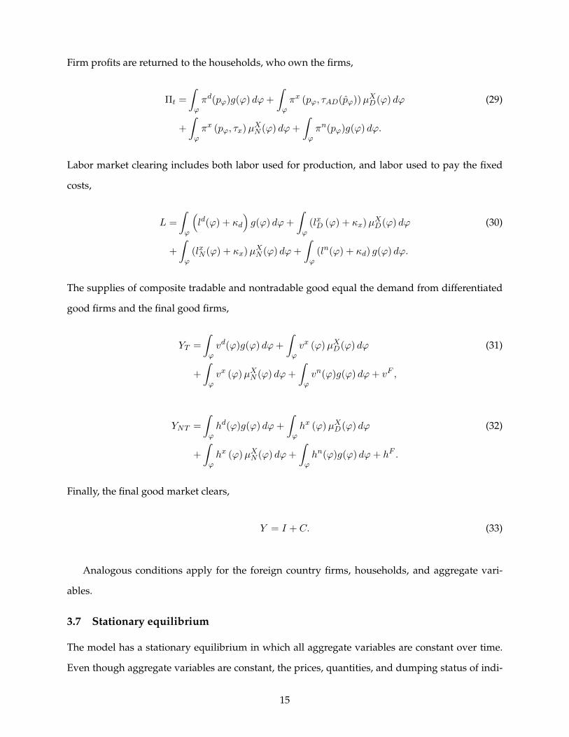
Firm profits are returned to the households, who own the firms,
Πt =
∫ϕπd(pϕ)g(ϕ) dϕ+
∫ϕπx (pϕ, τAD(pϕ))µXD(ϕ) dϕ (29)
+
∫ϕπx (pϕ, τx)µXN (ϕ) dϕ+
∫ϕπn(pϕ)g(ϕ) dϕ.
Labor market clearing includes both labor used for production, and labor used to pay the fixed
costs,
L =
∫ϕ
(ld(ϕ) + κd
)g(ϕ) dϕ+
∫ϕ
(lxD (ϕ) + κx)µXD(ϕ) dϕ (30)
+
∫ϕ
(lxN (ϕ) + κx)µXN (ϕ) dϕ+
∫ϕ
(ln(ϕ) + κd) g(ϕ) dϕ.
The supplies of composite tradable and nontradable good equal the demand from differentiated
good firms and the final good firms,
YT =
∫ϕvd(ϕ)g(ϕ) dϕ+
∫ϕvx (ϕ)µXD(ϕ) dϕ (31)
+
∫ϕvx (ϕ)µXN (ϕ) dϕ+
∫ϕvn(ϕ)g(ϕ) dϕ+ vF ,
YNT =
∫ϕhd(ϕ)g(ϕ) dϕ+
∫ϕhx (ϕ)µXD(ϕ) dϕ (32)
+
∫ϕhx (ϕ)µXN (ϕ) dϕ+
∫ϕhn(ϕ)g(ϕ) dϕ+ hF .
Finally, the final good market clears,
Y = I + C. (33)
Analogous conditions apply for the foreign country firms, households, and aggregate vari-
ables.
3.7 Stationary equilibrium
The model has a stationary equilibrium in which all aggregate variables are constant over time.
Even though aggregate variables are constant, the prices, quantities, and dumping status of indi-
15
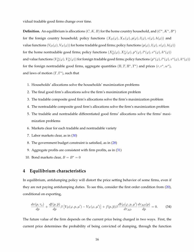
vidual tradable good firms change over time.
Definition. An equilibrium is allocations (C,K,B) for the home country household, and (C∗,K∗, B∗)
for the foreign country household; policy functions (XD(ϕ), XN (ϕ), p(ϕ), l(ϕ), v(ϕ), h(ϕ)) and
value functions (VD(ϕ), VN (ϕ)) for home tradable good firms; policy functions (p(ϕ), l(ϕ), v(ϕ), h(ϕ))
for the home nontradable good firms; policy functions (X∗D(ϕ), X∗N (ϕ), p∗(ϕ), l∗(ϕ), v∗(ϕ), h∗(ϕ))
and value functions (V ∗D(ϕ), V ∗N (ϕ)) for foreign tradable good firms; policy functions (p∗(ϕ), l∗(ϕ), v∗(ϕ), h∗(ϕ))
for the foreign nontradable good firms, aggregate quantities (Π, T,Π∗, T ∗) and prices (r, r∗, w∗),
and laws of motion (Γ,Γ∗), such that
1. Households’ allocations solve the households’ maximization problems
2. The final good firm’s allocations solve the firm’s maximization problem
3. The tradable composite good firm’s allocations solve the firm’s maximization problem
4. The nontradable composite good firm’s allocations solve the firm’s maximization problem
5. The tradable and nontradable differentiated good firms’ allocations solve the firms’ maxi-
mization problems
6. Markets clear for each tradable and nontradable variety
7. Labor markets clear, as in (30)
8. The government budget constraint is satisfied, as in (28)
9. Aggregate profits are consistent with firm profits, as in (31)
10. Bond markets clear, B = B∗ = 0
4 Equilibrium characteristics
In equilibrium, antidumping policy will distort the price setting behavior of some firms, even if
they are not paying antidumping duties. To see this, consider the first order condition from (20),
conditional on exporting,
dπ(p, τx)
dp+df(p, p)
dpβ[VD(ϕ, p, µ′) − VN (ϕ, µ′)
]+ f(p, p)β
dVD(ϕ, p, µ′)
dτAD
dτAD(p)
dp= 0. (34)
The future value of the firm depends on the current price being charged in two ways. First, the
current price determines the probability of being convicted of dumping, through the function
16

f(p, p). Second, the size of the antidumping duty is decreasing in the current price. This makes
the value of the firm paying antidumping duties also a function of p.
The first term on the left-hand side of (34) is the marginal change in current period profit from
a change in the current price. The second and third terms are the marginal change in the future
value of the firm.
For a firm that sets a price of at least p, the probability of being charged with dumping is
zero—which makes the second and third terns on the left-hand side of (34) zero—so the price
setting problem is static, leading to the familiar monopolistic competition pricing rule,
p = pm =mc(ϕ)
ρ. (35)
For firms whose productivity is so low that pm ≥ p, the optimal choice is to set the monopoly
price; antidumping policy does not distort the choices of these relatively unproductive firms.
Firms with high levels of productivity may find that pm ≤ p, which puts it at risk for being
charged with dumping. In this case, the firm chooses the price that solves (34), and the standard
monopolistic competition pricing rule is not optimal when the firm is in the region where f(p, p) is
decreasing. The firm will charge a price that is strictly greater than the monopolistic competition
price. This is a channel through which antidumping policy weakens competition in the domestic
market and does so in a way that is biased against productive firms.
Once a firm is found to be dumping, it is always optimal to set the monopoly price. Since the
probability of exiting the antidumping penalty phase is independent of the firm’s pricing decision,
a firm that is required to pay an antidumping duty will set its price according to (35) in order to
maximize the current period’s profits.
4.1 Equilibrium distribution of firms
In the stationary equilibrium the mass of each tradable firm type (exporting and paying antidump-
ing duties, exporting but not paying antidumping duties, not exporting but would pay antidump-
ing duties if exporting) is constant, although individual firms will be transiting between these
different states.
For firms with low enough productivity, it will never be profitable to export, even if they do
17

not face antidumping duties. This implies that, either g(ϕ) = µNXN (ϕ), and firms with productivity
ϕ never export, or the total mass of firms of type ϕ is distributed across exporting states, g(ϕ) =
µNXD (ϕ) + µXN (ϕ) + µXD(ϕ). The adding up constraint, along with the laws of motion in (24)–(27)
can be solved to yield the distribution over exporting firm types in the stationary equilibrium,
µXD(ϕ) =XD(ϕ)f(p(ϕ), p)
f(p(ϕ), p) + θg(ϕ) (36)
µXN (ϕ) =θ
f(p(ϕ), p) + θg(ϕ) (37)
µNXD (ϕ) = (1 −XD(ϕ))f(p(ϕ), p)
f(p(ϕ), p) + θg(ϕ) (38)
5 Calibration
The model is calibrated to the United States and a symmetric trading partner. Several of the firm
level statistics are taken from the 1992 census of manufacturers, so I use 1992 as the reference year
for all of the calibration moments. The calibration is summarized in table 1. The parameter ρ is
set so that the elasticity of substitution between varieties is 4; this is consistent with Broda and
Weinstein (2006). γ is chosen so that the elasticity of substitution between tradable and nontrad-
able goods is 0.5, as found in Stockman and Tesar (1995). The discount factor, β is chosen to be
consistent with a real annual interest rate of 4 percent; a period in the model is one year. The
preference parameter µT is set so that expenditure on nontradable goods makes up 62 percent of
total expenditure, as in the U.S. data. The annual depreciation rate of capital is 0.08, and capital’s
share of total income is 0.42, pinning down α.
The parameters ωN and ωT determine the input-output structure of the economy. I choose ωN
so that the nontradable goods make up 20 percent of output, as in the U.S. input-output table.
Analogously, I set ωT to match the share of tradable intermediate goods in output from the input-
output table. The distortions in the tradable good sector are transmitted to the nontradable good
sector through these input-output linkages.
The productivity distribution of potential entrants, g(ϕ), is assumed to be log normal. The
shape of the initial distribution is an important determinant in the shape of the equilibrium firm
size distribution, and Rossi-Hansberg and Wright (2007) document the log normality of the em-
ployment size distribution in manufacturing. The mean of the productivity distribution is nor-
18

Table 1: Baseline calibration.
Parameter Target Target Value
ρ elasticity of substitution between varieties 5γ elasticity of substitution between tradable and nontradable goods 0.5β annual interest rate (percent) 4.0δ depreciation rate 0.08µT share of nontradable expenditure in total expenditure 0.62α capital’s share of income 0.42ωN share of nontradable intermediates in output 0.20ωT share of tradable intermediates in output 0.41τx export-sales ratio, conditional on exporting (percent) 13.3κx export participation rate 0.20σϕ standard deviation of firm employment 175
Antidumping policy parameters
ε, λ standard deviation of antidumping duties (percent) 45median antidumping duties (percent) 43
θ duration of dumping penalty (years) 5
malized to be one, and the standard deviation, σϕ, is set so that the standard deviation of the
employment size distribution for tradable good firms is 175 workers, as in the census of manufac-
turers. The non-antidumping ad valorem trade cost, τx, is chosen so that the average export-sales
ratio of firms that export is 13.3 percent, as reported in the census of manufacturers. The fixed cost
of exporting, κx, is set so that 20 percent of all tradable good firms export.
The functional form for the antidumping policy is
f(p, p) =
λ+ (1 − λ) (1 − (p/p)ε) if p < p
0 if p ≥ p
In the baseline calibration I assume that the fair value price, p, is the CES price of tradable goods
produced by domestic firms in the importing country. The parameters ε and λ control the probabil-
ity of being charged with dumping relative to the price charged by the exporter. These parameters
are chosen to match the median and the standard deviation of the antidumping duties levied in
the model with that in the data. Lastly, the duration of antidumping duties is set to 5 years, by
setting θ = 0.20, consistent with the evidence presented in Cadot et al. (2007).
19

Figure 3: Distribution of antidumping measures in the model and the U.S. data.
50 100 150 200 250 300 350 4000.0
0.1
0.2
0.3
0.4
0.5
0.6
0.7
Antidumping duty (percent)
Fra
ctio
n o
f o
bse
rve
d d
uti
es
model
data
If figure 3 I plot the distribution of U.S. antidumping duties in the data and the model. The
model does a reasonably good job of capturing the distribution of antidumping duties observed
in the data. The model is able to generate enough small antidumping duties through the “bad
luck” dumping probability, λ. If the probability of being punished for dumping is only a function
of the price being charged, the model will not generate many small antidumping penalties.
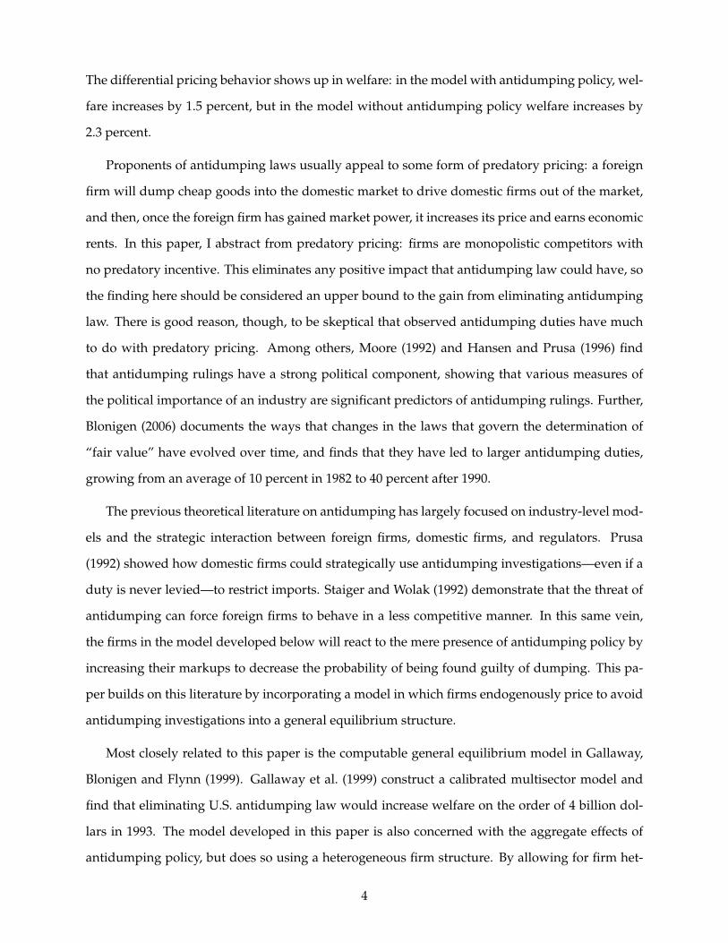
The estimated antidumping probability function, f(p, p) is plotted in figure 4. The horizontal
axis is the ratio of the firm’s price to the fair value price. When this ratio is greater or equal to 1,
the firm is in no danger of being punished for dumping. As the firm’s price falls relative to the
fair value price, the probability of being punished is increasing. Overall, the probability of being
punished for dumping is quite small, less than one percent.
The distribution over firms that export, as well as the implied probability of being convicted
of dumping, is plotted in figure 5 as function of the underlying productivity of the firm. In this
figure I plot the probability of being punished for dumping both at the firm’s optimal price and
and its static monopolist’s price. The probability at the optimal price is always lower than at the
monopolist’s price because the firm chooses to charge a higher price in equilibrium to partially
reduce the probability of being punished for dumping. The difference between the two probabili-
ties is increasing in the productivity of the firm: Antidumping policy creates larger distortions for
20

Figure 4: Antidumping probability function.
0.2 0.3 0.4 0.5 0.6 0.7 0.8 0.9 10.08
0.09
0.10
0.11
0.12
0.13
0.14
0.15
0.16
0.17
Firm price/fair value price
Pro
ba
bil
ity
of
du
mp
ing
pe
na
lty
(p
erc
en
t)
more productive firms.
Figure 5: Distribution of firm types and equilibrium probability of antidumping penalty.
2 4 6 8 10 12 14 16 18 200.05
0.10
0.15
0.20
prob. at monopolist price
prob. at optimal price
distribution of firmsPro
bab
ilit
y o
f d
um
pin
g p
en
alt
y (
pe
rce
nt)
Firm productivity
0.0
0.1
0.2
0.3
0.4
0.5
0.6
0.7
Mea
sure
of
firm
s (x
10
0)
6 The aggregate impact of antidumping policy
How, and by how much, does U.S. antidumping policy distort trade? To answer this question I
consider two counterfactuals. In the first, I keep all the other parameters fixed but set the value of
21
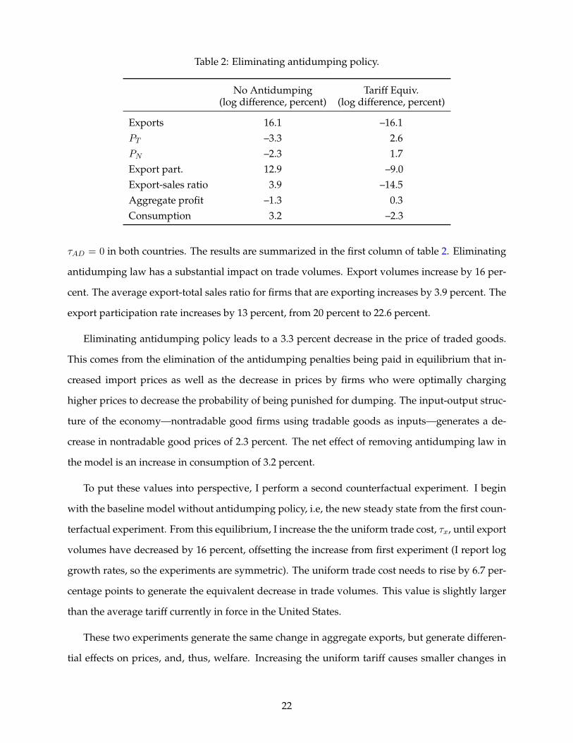
Table 2: Eliminating antidumping policy.
No Antidumping Tariff Equiv.(log difference, percent) (log difference, percent)
Exports 16.1 –16.1PT –3.3 2.6PN –2.3 1.7Export part. 12.9 –9.0Export-sales ratio 3.9 –14.5Aggregate profit –1.3 0.3Consumption 3.2 –2.3
τAD = 0 in both countries. The results are summarized in the first column of table 2. Eliminating
antidumping law has a substantial impact on trade volumes. Export volumes increase by 16 per-
cent. The average export-total sales ratio for firms that are exporting increases by 3.9 percent. The
export participation rate increases by 13 percent, from 20 percent to 22.6 percent.
Eliminating antidumping policy leads to a 3.3 percent decrease in the price of traded goods.
This comes from the elimination of the antidumping penalties being paid in equilibrium that in-
creased import prices as well as the decrease in prices by firms who were optimally charging
higher prices to decrease the probability of being punished for dumping. The input-output struc-
ture of the economy—nontradable good firms using tradable goods as inputs—generates a de-
crease in nontradable good prices of 2.3 percent. The net effect of removing antidumping law in
the model is an increase in consumption of 3.2 percent.
To put these values into perspective, I perform a second counterfactual experiment. I begin
with the baseline model without antidumping policy, i.e, the new steady state from the first coun-
terfactual experiment. From this equilibrium, I increase the the uniform trade cost, τx, until export
volumes have decreased by 16 percent, offsetting the increase from first experiment (I report log
growth rates, so the experiments are symmetric). The uniform trade cost needs to rise by 6.7 per-
centage points to generate the equivalent decrease in trade volumes. This value is slightly larger
than the average tariff currently in force in the United States.
These two experiments generate the same change in aggregate exports, but generate differen-
tial effects on prices, and, thus, welfare. Increasing the uniform tariff causes smaller changes in
22

prices compared to the antidumping policy. This is because the antidumping policy targets firms
that charge low prices. These low-priced goods have large shares in the economies expenditure,
causing larger aggregate effects.
6.1 Antidumping and New Trading Partners
The last 20 years have been marked by the rise of the developing world in global trade. Per-
haps unsurprisingly, these countries have become major targets for antidumping complaints:
complaints against China, alone, account for more than 20 percent of all antidumping investiga-
tions initiated since 1995 and almost 40 percent of cases initiated over this period were complaints
against low income countries. Exports from low wage countries generate welfare gains from lower
priced goods, but also increase competition for domestic producers. In this section I consider the
introduction of new trading partners into the model and study the differential impacts in a model
with and without antidumping policy.
[To be finished.]
7 Conclusion
As multilateral trade agreements have limited the ways that policy makers can restrict interna-
tional trade, antidumping complaints have become an important method for impeding imports.
In this paper I set out to determine the welfare costs of antidumping policy and the ways in which
antidumping policy differs from standard, uniformly applied tariffs. I find that U.S. antidump-
ing policy lowers total consumption by about 3 percent, and distorts aggregate trade to the same
extent as a 7 percent tariff. Since antidumping law targets firms who charge low prices, these poli-
cies generate a friction that increases with firm productivity, increasing the impact of antidumping
policy relative to standard tariffs.
The literature that has studied the effects of antidumping law have largely done so in the
context of industry-level dynamic games. While these papers have yielded important insights
into the behavior of firms, these models are generally too complex to use in an aggregate general
equilibrium model. In order to study the aggregate effects of antidumping law, I develop a model
of antidumping that, while still tractable, incorporates several of the key properties of current
antidumping law.
23

The tractability of the model of antidumping policy developed here makes it useful for study-
ing the effects of antidumping in more complex models. The incomplete pass through of the
falling marginal cost in section 6.1 suggests that antidumping law would lead to the incomplete
pass through of transitory business cycle shocks as well. Modifying the model developed here to
include aggregate shocks to productivity or the money supply is a promising avenue for future
study.
24

ReferencesBlonigen, Bruce A., “Evolving Discretionary Practices of U.S. Antidumping Activity,” Canadian
Journal of Economics, August 2006, 39 (3), 874–900.
and Jee-Hyeong Park, “Dynamic Pricing in the Presence of Antidumping Policy: Theoryand Evidence,” The American Economic Review, 2004, 94 (1), 134–154.
Broda, Christian and David E. Weinstein, “Globalization and the Gains from Variety,” The Quar-terly Journal of Economics, 2006, 121 (2), 541–85.
Cadot, Olivier, Jaime de Melo, and Bolormaa Tumurchudur, “Anti-Dumping Sunset Reviews:The Uneven Reach of WTO Disciplines,” CEPR Discussion Papers 6502, C.E.P.R. DiscussionPapers 2007.
Finger, J. Michael, “The Origins and Evolution of Antidumping Regulation,” in J. Michael Finger,ed., Antidumping, Ann Arbor: The University of Michigan Press, 1993, pp. 13–34.
Gallaway, Michael P., Bruce A. Blonigen, and Joseph E. Flynn, “Welfare Costs of the US An-tidumping and Countervailing Duty Laws,” Journal of International Economics, 1999, 49 (2),211–244.
Guner, Nezih, Gustavo Ventura, and Xu Yi, “Macroeconomic Implications of Size-DependentPolicies,” Review of Economic Dynamics, October 2008, 11 (4), 721–744.
Hansen, Wendy L. and Thomas J. Prusa, “Cumulation and ITC Decision-Making: The Sum of theParts Is Greater than the Whole,” Economic Inquiry, 1996, 34 (4), 746–769.
Lindsey, Brink and Daniel J. Ikenson, Antidumping Exposed: The Devilish Details of Unfair TradeLaw, Washington: CATO Institute, 2003.
Moore, Michael O., “Rules or Politics?: An Empirical Analysis of ITC Anti-dumping Decisions,”Economic Inquiry, 1992, 30 (3), 449–466.
Obama, Barack, “Remarks by The President in State of Union Address,” The White House, Office ofthe Press Secretary, 2012.
Prusa, Thomas J., “Why Are so Many Antidumping Petitions Withdrawn?,” Journal of InternationalEconomics, 1992, 33, 1–20.
Restuccia, Diego and Richard Rogerson, “Policy Distortions and Aggregate Productivity withHeterogeneous Plants,” Review of Economic Dynamics, October 2008, 11 (4), 707–720.
Rossi-Hansberg, Esteban and Mark L. J. Wright, “Establishment Size Dynamics in the AggregateEconomy,” American Economic Review, 2007, 97 (5), 1639–1666.
Staiger, Robert W. and Frank A. Wolak, “The Effect of Domestic Antidumping Law in the Pres-ence of Foreign Monopoly,” Journal of International Economics, 1992, 32, 265–87.
Stiglitz, Joseph E., “Dumping on Free Trade: The U.S. Import Trade Laws,” Southern EconomicJournal, 1997, 94 (2), 402–424.
Stockman, Alan C. and Linda L Tesar, “Tastes and Technology in a Two-Country Model of theBusiness Cycle: Explaining International Comovements,” American Economic Review, 1995, 85(1), 168–85.
25