The Advanced Regional Prediction System (ARPS), …kkd.ou.edu/ARPSPaperIII.pdfAdvanced Regional Prediction System of the Center for Analysis and Prediction of Storms at the University

Meteorol Atmos Phys 82, 139–170 (2003)DOI 10.1007/s00703-001-0595-6

1 Center for Analysis and Prediction of Storms, University of Oklahoma, Norman, OK 73019, USA2 School of Meteorology, University of Oklahoma, Norman, OK 73019, USA

The Advanced Regional Prediction System (ARPS),storm-scale numerical weather predictionand data assimilation

Ming Xue1;2, Donghai Wang1;�, Jidong Gao1, Keith Brewster1,and Kelvin K. Droegemeier1;2

With 12 Figures

Received May 7, 2001; revised October 15, 2001Published online: November 21, 2002 # Springer-Verlag 2002

Summary

In this paper, we first describe the current status of theAdvanced Regional Prediction System of the Center forAnalysis and Prediction of Storms at the University ofOklahoma. A brief outline of future plans is also given. Tworather successful cases of explicit prediction of tornadicthunderstorms are then presented. In the first case, a seriesof supercell storms that produced a historical number oftornadoes was successfully predicted more than 8 hours inadvance, to within tens of kilometers in space with ini-tiation timing errors of less than 2 hours. The general be-havior and evolution of the predicted thunderstorms agreevery well with radar observations. In the second case,reflectivity and radial velocity observations from Dopplerradars were assimilated into the model at 15-minute inter-vals. The ensuing forecast, covering a period of several hours,accurately reproduced the intensification and evolution ofa tornadic supercell that in reality spawned two tornadoesover a major metropolitan area. These results make usoptimistic that a model system such as the ARPS will beable to deterministically predict future severe convectiveevents with significant lead time. The paper also includes abrief description of a new 3DVAR system developed in theARPS framework. The goal is to combine several steps ofDoppler radar retrieval with the analysis of other data typesinto a single 3-D variational framework and later toincorporate the ARPS adjoint to establish a true 4DVAR

data assimilation system that is suitable for directlyassimilating a wide variety of observations for flows rang-ing from synoptic down to the small nonhydrostatic scales.

1. Introduction

In 1989, the Center for Analysis and Predictionof Storms (CAPS) was established at the Univer-sity of Oklahoma as one of the National ScienceFoundation’s first 11 Science and Technology(S&T) Centers. Its formal mission was to demon-strate the practicability of storm-scale numericalweather prediction and to develop, test, and vali-date a regional forecast system appropriate foroperational, commercial, and research applica-tions. Its ultimate vision was to make available afully functioning storm-scale NWP system (Lilly,1990; Droegemeier, 1990).

To achieve the above mission, an advancedprediction model system was needed. It wasdecided that this model had to meet a numberof criteria. First, it had to be able to assimilate,through modern data assimilation strategies, newdata of higher temporal and spatial density (e.g.,those from the WSR-88D Doppler radar net-work) than had traditionally been available.

� Current address: NASA Langley Research Center, Hampton,

VA 23681-2199.

Second, the model had to serve as an effectivetool for studying the dynamics and predictabilityof storm-scale weather in both idealized andrealistic numerical weather prediction (NWP)settings. It must also handle atmospheric phe-nomena ranging from regional scales down tomicro-scales as interactions across this spectrumare known to have profoundly important impactson storm-scale phenomena. The model also hadto be able to run efficiently on modern parallelcomputing platforms. These needs required thatthe model have a flexible and general dynamicand computational framework and include com-prehensive physical processes.

Despite the availability of a number of non-hydrostatic research models at the time of its es-tablishment, CAPS chose to develop an entirelynew model for a number of reasons. First, mostexisting models were initially developed by indi-viduals for specific research problems and theyhave since undergone considerable modificationsand thus reflect the disparate programmingstyles of each contributor. Some of these mod-els evolved from their hydrostatic predecessorsstarted decades ago. Such codes are often poorlydocumented and therefore require substantialefforts to learn and are even harder to modifyfor the rapid investigation of scientific ideas. Sec-ond, such model codes were developed mostly onolder generation computers and in many casesrequire substantial re-tooling for modern, espe-cially distributed-memory, parallel processors.

Third, the assimilation of observational dataon the thunderstorm scale is particularly chal-lenging, especially with four-dimensional varia-tional method based on the adjoint technique(Kapitza, 1991; Sun et al, 1991). The creationof the adjoint code is a tedious process proneto error and can be greatly simplified by a carefuldesign of the forward model. Further, care indeveloping the forward model can also greatlyfacilitate the use of automated tools for obtainingthe adjoint (Talagrand, 1991; Bischof et al,1992). Finally, a well-designed model frame-work will also facilitate the implementation ofmore accurate numerical techniques and modelphysics.

For the above reasons, an entirely new, three-dimensional, nonhydrostatic model system knownas the Advanced Regional Prediction System(ARPS) was developed. It is a comprehensivemulti-scale prediction system that includes dataingest, quality control, and objective analysispackages, single-Doppler radar parameter retriev-al and data assimilation procedures, the predic-tion model, as well as post-processing packagesand validation tools (Fig. 1). By the end of itspredetermined 11-year life as a NSF S&T center,we believe that CAPS has largely accomplishedits original ambitious goals. Currently, CAPS con-tinues as a center under the support of a numberof initiatives and grants.

The numerical prediction component of theARPS is a three-dimensional, nonhydrostatic

Fig. 1. The principal components of the ARPS system

140 M. Xue et al

compressible model formulated in generalizedterrain-following coordinates. It is designed fromthe beginning to run on computing platforms rang-ing from single-processor scalar workstations tomassively parallel scalar or vector processors.Guided by modern software engineering theoriesand practices, the entire system is written in aconsistent style and is easy to use, extend andmaintain. The code is also extensively docu-mented and the system has served as an effectiveresearch, educational and prediction tool for avariety of applications by users throughout theworld. The ARPS contains a comprehensive phys-ics package and a self-contained data analysis,radar data retrieval and assimilation system. Ithas been subjecting to real-time weather predic-tion testing over several regions since mid-90s(e.g., Droegemeier et al, 1996; Xue et al,1996a; Droegemeier, 1997; Carpenter et al, 1999;Shin et al, 1998). In the spring 1998, ARPS par-ticipated in a unique multi-model mesoscale en-semble prediction experiment organized by theCAPS, and the results are summarized in Houet al (2001).

The ARPS, that existed in the form of a typicalcloud model, was first made available to thepublic in 1992 (CAPS, 1992). The first compre-hensive description of the formulation, numeri-cal solution methods, physics parameterizations,computational implementation and configurationinstructions for the system is given in the ARPSVersion 4.0 User’s Guide (Xue et al, 1995). Morerecent improvements and model verifications aredescribed in Xue et al (2000; 2001). In this paper,we describe in Sect. 2 the current capabilities ofthe ARPS. Two sets of predictions at thunder-storm-resolving resolutions are presented inSects. 3 and 4. The first case starts from the anal-ysis of conventional data and predicts the initia-tion and evolution of a series of tornadicthunderstorms. In the second case, a rapid updateassimilation cycle, including the analysis ofcloud fields using Doppler radar data, is em-ployed and the model successfully predicts thedevelopment and evolution of pre-existing thun-derstorms. Section 5 describes the recently devel-oped ARPS 3DVAR system and discusses certainissues of data assimilations at the small nonhy-drostatic scales, in particular those related to theuse of radar data. Section 5 also presents anexample analysis using the 3DVAR system and

its comparison with the analysis using ARPSData Analysis System (ADAS). Section 6 con-cludes with an overall summary of the paper.

2. Current features of the ARPS system

ARPS version 4.0 was officially released inmid-1995. Since then, many improvements havebeen made to the system and many sub-releaseswere made available on the CAPS anonymousFTP server (ftp:==ftp.caps.ou.edu=ARPS). In late2000, the entire system was converted to Fortran90 free-format using an automatic code convertercustomized to conform the ARPS Fortran 90coding standard. Dynamic memory allocationwas subsequently implemented manually for allprograms. Significant development and improve-ments with the ARPS system since the Version 4release include:

– A completely new real-time data ingest andanalysis system (ADAS, Brewster, 1996) ca-pable of handling a variety of data sources,including raw and retrieved Doppler radarand satellite data;

– A cloud analysis component in the ADAS thatcreates three-dimensional fields of cloudwater, rainwater and improved fields of watervapor and temperature (Zhang et al, 1998;Zhang and Carr, 1998; Zhang, 1999);

– An integrated package for single-Dopplervelocity and thermodynamic retrievals to-gether with the associated variational adjust-ment procedures (Shapiro et al, 1995a; 1995b;1996; Weygandt et al, 1998);

– A long and short-wave radiation packagebased on that of the NASA Goddard SpaceFlight Center (Chou, 1990; 1992; Chou andSuarez, 1994);

– The Skamarock adaptive grid refinement thatsupports multiple level two-way interactivegrid nesting and run-time addition, removaland movement of nested grids (Skamarockand Klemp, 1993; Xue et al, 1993);

– Kain–Fritsch (Kain and Fritsch, 1993) cumu-lus parameterization;

– A non-local PBL parameterization based on1.5-order TKE turbulence scheme (Xue et al,1996b);

– A sophisticated three-phase ice microphysics(Lin et al, 1983; Tao et al, 1989), along with

ARPS, storm-scale numerical weather prediction and data assimilation 141

the Schultz (1995) simplified ice microphys-ics, in addition to the previously availableKessler warm-rain scheme;

– Inclusion of snow cover and refinement of theland surface-vegetation model;

– High resolution (as fine as 100 m) terrain,land-use and land-cover data bases and theoption to define multiple soil types in eachgrid cell to take advantage of the high-resolu-tion soil-type data base;

– An ensemble prediction component using thescaled lagged averaged forecasting (SLAF)technique for generating initial and bound-ary condition perturbations (Ebisuszki andKalnay, 1991; Hou et al, 2001);

– A flux-corrected transport (FCT) monotonicscalar advection option plus an efficient posi-tive-definite advection scheme based on leap-frog-centered scheme (Zalesak, 1979; Lafore,1998; Xue et al, 2000) in addition to the qua-dratically conserving second- and fourth-orderadvection (Xue and Lin, 2001);

– Options for monotonic high-order numericaldiffusion (Xue, 2000);

– A radiation top-boundary condition with arelaxed limitation at the top lateral boundaries(Xue et al, 2000);

– Map factor in dynamic equations and provi-sion for stretching in horizontal as well asthe vertical directions (Xue et al, 2000);

– The use of the full density, instead of base-state density, in the pressure gradient forceterms and the elimination of approximationsin early versions of the dynamic equations;

– Support for gridded data sets from variousoperational models (e.g., RUC, ETA and AVN),the NCAR-NCEP global reanalysis as well asARPS’s own forecast to provide the analysisbackground and boundary conditions;

– Streamlined support for distributed memoryplatforms (e.g., the Cray T3E, SGI Origin;IBM SP, and NEC SX series, and workstationclusters including Linux PCs) via a messagepassing interface (MPI);

– Significant code optimization, including thatachieved by removing differencing operatorsand by using lookup tables for expensivemathematical functions;

– A soil model initialization procedure usingantecedent precipitation index (API, see e.g.,example of use in Xue et al, 1998) or NCEP

model fields, and an option to perform precy-cling of the soil model to obtain a balancedinitial condition;

– A sophisticated Perl-based automated proce-dure for real-time data ingest, analysis andprediction control and web posting;

– Significantly enhanced graphics post-analysisprograms;

– Support of several additional data formats(e.g., Vis5D, GRIB, GrADS, HDF, NetCDF)and their associated display and visualizationtools;

– Several new Doppler radar analysis and re-trieval schemes (Gao et al, 1999; 2001b;2001c; Shapiro et al, 1999) and the associatedpre-processing programs;

– A phase-correction scheme for adjusting themodel or model-background states for phaseor position errors in the forecast based onradar and other observations (Brewster, 1999;Brewster, 2002a; 2002b);

– A version of 4DDA scheme based on the full-model adjoint (Wang et al, 1995; 1997; Gaoet al, 1998);

– A version of three-dimensional variationaldata assimilation system (3DVAR, Gao et al,2001a).

A fully tested, Fortran 90 version was releasedin 2002 as ARPS version 5.0. The primary focusfor the next few years at CAPS will be the con-tinued development of the three-dimensional var-iational (3DVAR) system that will incorporateradar data retrievals and the analysis of all otherdata types in one single unified variational frame-work. The 3DVAR system will be a natural suc-cessor to the current ADAS and will serve as thefoundation for a complete 4DVAR system basedon the full model adjoint. We will also continueto improve the model physics, including those forprecipitation and land surface processes. We willcalibrate and improve the current and futureversions of the land surface model in the ARPSusing direct soil temperature and moisture mea-surements from the Oklahoma Mesonet, anddesign and test a soil state variable retrievalsystem based on the soil model and its adjoint.In addition, we will implement a new two-waynesting capability that will run on distributedmemory parallel platforms. Information on allaspects of the ARPS system can be found at

142 M. Xue et al

http:==www.caps.ou.edu=ARPS. In the followingtwo sections, we will present results from theARPS as applied to explicit prediction of thun-derstorm-scale weather. Before moving on to thenext sections, we point out that the unique fea-tures in small-scale data assimilation, especiallyof Doppler radar data, careful computationaldesign and parallel implementation of the modelsystem from the beginning (Droegemeier et al,1995; Johnson et al, 1994), and the choice ofthe state-of-the-science numerical techniquesand physics parameterizations made the modeluniquely suitable for our mission, namely,storm-scale research and NWP.

3. ARPS prediction of the January 21–23,1999 Arkansas tornado outbreak case

3.1. Case introduction

A major tornado outbreak occurred during theafternoon and evening of January 21, 1999 inthe state of Arkansas (AR), in the central U.S.Fifty-six tornadoes were reported statewide withthe strongest tornadoes rated F3 (maximumwinds 71 ms� 1 to 92 ms� 1) on the Fujita scale.Most of the tornadoes occurred between 4 and11 pm CST, or between 22 UTC January 21and 05 UTC January 22. Eight people were killedby the tornadoes. It is believed to be the largesttornado outbreak in Arkansas. The number oftornadoes in this single event is nearly triplethe historical average number of 21 per year inthe state. The fact that this event occurred inJanuary makes it even more unusual. In fact, thiscase had the most tornadoes ever in a single statefor the month of January.

This event occurred during the extended pe-riod of CAPS AMS-99 (1999 American Meteo-rological Society Annual Meetings) real-timeforecasting experiment, when CAPS was runningthe model on triple nested grids with the finestgrid at 3-km grid spacing. Further study of thiscase has been made after the event, using largerdomains for all three grids and higher resolutionsfor the intermediate (6-km) and finest (2-km)grids, and extending the forecast to 48 hours.Furthermore, intermittent data assimilation cy-cles are performed at the coarsest-resolution(32-km) grid. The goal is to examine the model’sability to forecast the entire sequence of events

down to the convective-storm scales, includingstorms with strong rotating characteristics duringthe period of the tornado outbreak, and later theorganization of storms leading to a long-livedpropagating squall line. The results should alsogive insight into the predictability of events onthe convective-storm scales. Furthermore, a suc-cessful prediction of the sequence of eventsoffers us a valuable data set that can be furtheranalyzed for understanding the dynamic and phys-ical processes involved. Sensitivity experimentscan be performed to further our understanding.

The synoptic-scale features and events ofthis case have been documented in Xue (2001),together with the prediction results on the 32-kmand 6-km grid. In summary, the tornado outbreakoccurred ahead of a deepening upper-level troughwhose trough line was located over westernTexas (TX). The upper-level wind backed slight-ly from west–southwesterly to southwesterly 12UTC through 00 UTC. At the surface, a low thatwas over the Rockies earlier descended to the lee(east) side and expanded in size. The centerremained in southwestern Oklahoma (OK) forthis 12-hour period. At 00 UTC, January 22, asurface cold front was found extending from thesurface low center to southwest (SW) TX, whilea quasi-stationary front extended from the lowcenter northeastward then eastward throughMissouri (MO) all the way to the east coast ofthe United States. The area of tornado outbreakwas therefore located in warm sector of the sur-face low, several hundreds of km ahead of thesurface cold front. South of a SW–NE diagonalline bisecting Arkansas, the low-level flow wassoutherly for the entire 12-hour period and theobserved CAPE reached 2000 J=kg south of thisline. During the several hours surrounding 00UTC January 22, most of the supercell stormsthat spawn tornadoes moved northeastwardsalong this diagonal line. In the 36 hours follow-ing the tornado outbreak, subsequent convectionorganized into an intense long-lasting squall linethat moved east across much of eastern US, andfinally into the Atlantic Ocean.

3.2. ARPS model forecast

The ARPS forecasts on the 32- and 6-km gridsstarting from 12 UTC January 21 and valid at 00UTC January 22 and at 12 UTC January 23 were


presented in Xue et al (2001), along with a briefdiscussion on the results. At the end of that peri-od, a squall line that matched very well withobservations was obtained that extended north–south across the entire east coast of the US. Inthis paper, we focus on the results of the nested2-km grid, for the period spanning the tornadooutbreak. Particular attention is paid to the tim-ing, location and characteristics of the model pre-dicted storms, as compared to radar observations.

All runs started from 12 UTC, January 21,1999. A 24-h long hourly intermittent data as-similation cycle was performed on the 32-km gridto achieve the best reproduction of the synopticscale state of the atmosphere. The 6-km gridstarted from the 12 UTC ADAS analysis andwas forced by the 32-km solutions at the lateralboundaries. All available observations, including

data from the Oklahoma Mesonet data and thecentral-plains wind profiler demonstration net-work were used. The 2-km grid was initializedfrom interpolated 6-km analysis, without furtheraddition of data. Because the initial time precedesthe times with significant convective storms in theprimary area of interest, no radar data (at leastthose in precipitation mode) were available foruse in the initial analysis. It is therefore up tothe model to initiate the convective storms severalhours after the model initial time. Additionaldetails on the model configuration can be foundin Xue et al (2001).

As an overview, we first present in Fig. 2 acomparison of the simulated composite radarreflectivity field from the 32-km model with theobserved one. It can be seen in the portion ofdomain having radar observations, the model

Fig. 2. Observed radar composite reflectivityfield (a), and ARPS (b) surface winds, mean sea-level pressure (contours) and composite reflec-tivity field (shaded contours) at 00 UTC January22, 1999 on the 32-km grid, corresponding to12 h model time. The domain in (a) correspondsto the thick dashed box in (b). The two solidboxes in (b) indicate the 6- and 2-km domains

144 M. Xue et al

reflectivity pattern matches very well with theobserved one. This includes an elongated precipi-tation region across the SW–NE axis of AR andthe generally east–west oriented precipitationbands associated with a quasi-stationary front tothe north. The areas of light precipitation overthe Rockies, eastern North Dakota into westernMinnesota, and over New Jersey and the sur-rounding region are also well reproduced. How-ever, the model, at 32 km resolution, is not capableof producing high reflectivity values comparableto the observed ones in Arkansas, where tornadicthunderstorms were at their full strength at thistime. It should be noted that the Kain–Fritschcumulus parameterization option was used to-gether with the explicit ice microphysics schemeon this grid. The reflectivity field presented doesnot include the parameterized convective precipi-tation. The field of total precipitation rate (notshown), however, does match the reflectivity pat-tern closely at this time, with the most noticeabledifference being at the southern end of diagonalreflectivity region where additional parameter-ized precipitation was found. Cumulus parameter-ization was not used on either the 6- or 2-km grid.

3.3. Comparisons of 2-km resolution modelforecasts with radar observations

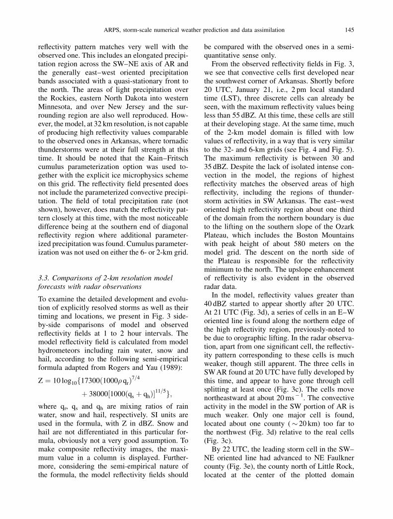
To examine the detailed development and evolu-tion of explicitly resolved storms as well as theirtiming and locations, we present in Fig. 3 side-by-side comparisons of model and observedreflectivity fields at 1 to 2 hour intervals. Themodel reflectivity field is calculated from modelhydrometeors including rain water, snow andhail, according to the following semi-empiricalformula adapted from Rogers and Yau (1989):

Z ¼ 10 log10f17300ð1000� qrÞ7=4

þ 38000½1000ðqs þ qhÞ11=5g;

where qr, qs and qh are mixing ratios of rainwater, snow and hail, respectively. SI units areused in the formula, with Z in dBZ. Snow andhail are not differentiated in this particular for-mula, obviously not a very good assumption. Tomake composite reflectivity images, the maxi-mum value in a column is displayed. Further-more, considering the semi-empirical nature ofthe formula, the model reflectivity fields should

be compared with the observed ones in a semi-quantitative sense only.

From the observed reflectivity fields in Fig. 3,we see that convective cells first developed nearthe southwest corner of Arkansas. Shortly before20 UTC, January 21, i.e., 2 pm local standardtime (LST), three discrete cells can already beseen, with the maximum reflectivity values beingless than 55 dBZ. At this time, these cells are stillat their developing stage. At the same time, muchof the 2-km model domain is filled with lowvalues of reflectivity, in a way that is very similarto the 32- and 6-km grids (see Fig. 4 and Fig. 5).The maximum reflectivity is between 30 and35 dBZ. Despite the lack of isolated intense con-vection in the model, the regions of highestreflectivity matches the observed areas of highreflectivity, including the regions of thunder-storm activities in SW Arkansas. The east–westoriented high reflectivity region about one thirdof the domain from the northern boundary is dueto the lifting on the southern slope of the OzarkPlateau, which includes the Boston Mountainswith peak height of about 580 meters on themodel grid. The descent on the north side ofthe Plateau is responsible for the reflectivityminimum to the north. The upslope enhancementof reflectivity is also evident in the observedradar data.

In the model, reflectivity values greater than40 dBZ started to appear shortly after 20 UTC.At 21 UTC (Fig. 3d), a series of cells in an E–Woriented line is found along the northern edge ofthe high reflectivity region, previously-noted tobe due to orographic lifting. In the radar observa-tion, apart from one significant cell, the reflectiv-ity pattern corresponding to these cells is muchweaker, though still apparent. The three cells inSWAR found at 20 UTC have fully developed bythis time, and appear to have gone through cellsplitting at least once (Fig. 3c). The cells movenortheastward at about 20 ms� 1. The convectiveactivity in the model in the SW portion of AR ismuch weaker. Only one major cell is found,located about one county (� 20 km) too far tothe northwest (Fig. 3d) relative to the real cells(Fig. 3c).

By 22 UTC, the leading storm cell in the SW–NE oriented line had advanced to NE Faulknercounty (Fig. 3e), the county north of Little Rock,located at the center of the plotted domain


(marked by letter L in Fig. 3a). It spawned thefirst two F2 tornadoes and caused 6 injuries inone of the homes according to the NationalWeather Service’s storm data. Outside this line,a few weaker isolated storms formed to the east.In the model, most intense storms are found nearthe northern state boundary, a result of the north-ward propagation of the line found near thenorthern boundary at 21 UTC (Fig. 3f). Clearlythese storms were over-predicted by the model.

Corresponding to the actual intense storms,which extended from the domain center to theSW corner, are model storms that are still at theirformative stages in SW–NE lines, about 1 to 2counties to the northwest. The individual cells inthe model moved northeastward, in agreementwith the observed storm motion (Fig. 3f). Majordevelopment occurred in the model in the 15-minute period between 2200–2215 UTC, withseveral new cells appearing near the SW cornerof the domain, close to the southern state bound-ary while those cells seen at 22 UTC near the SWcorner of Arkansas began to intensify. By 22:30UTC, a series of cells organized in a SSW–NNEoriented line were already exhibiting hook-shaped echoes indicating significant updraft rota-tion (not shown). By 23 UTC, both the stormsoriginating in the southwest and those to thenorth have become fully developed (Fig. 3h).Their reflectivity fields all exhibit a strong reflec-tivity gradient on their southwest flanks withmany exhibiting hook-like appendages while thesurface wind fields show strong convergence intothe storms.

The first F3 tornado was reported at around22:30 UTC in Dallas County, located in thesouth-central part of the domain (indicated byletter D in Fig. 3g), where a relatively isolatedstorm is clearly depicted. In the next half an hour,three more F3 tornadoes were reported in White,Independence and Monroe counties (indicated byletters W, I and M respectively in Fig. 3g), eachcorresponding to a major storm found in Fig. 3g.Many more weaker tornadoes were also reported.

The model solution showed a marked increase inthe low level vorticity after 22 UTC (not shown)which matched, or slightly lagged in the time,this first wave of intense tornado activity.

At 23 UTC, about a dozen storm cells can beidentified both in radar observations and in themodel, and both model and real storms exhibitisolated supercell storm characteristics with rota-tion more readily identifiable in the model.Zoomed-in plots of observed reflectivity fieldsalso show hook-echo shapes and strong reflectiv-ity gradients in some of the cells.

For the next three hours, from 23 UTC to 02UTC January 22, both observation and modelshowed new cells being continually generatedat the south end of the convective line while oldercells moved along the diagonal axis across thestate. In the model, while the cells moved inthe correct directions, the line orientation isrotated a bit toward a north–south orientationrelative to the observations, a result of the cellorigination points being a couple of counties toofar to the east and the convection to the northbeing initially displaced to the west. By the endof this three-hour period, the line in the modelhas turned more into the SW–NE orientation. Asmore cells were created through splitting processand the low-level cold pool spread, the storms inboth the model and the real world became closerto each other and some, especially the older onesin the northern part, started to join together, cre-ating connected line segments. At 02 UTC, thesouthern end of the observed and modeled lineswere still touching the south–southwest state cor-ner of Arkansas (Fig. 3k and Fig. 3l).

In the two hours following 02 UTC, the trendfor the cells to merge and form a continuous linecontinued both in the model and in the real world(Fig. 3m and Fig. 3n). New cells stopped formingafter 02 UTC (8 pm local time) as the boundarylayer cooled after sunset, decreasing CAPE andincreasing convective inhibition (CIN). By 04UTC, the southern end of the primary line istwo-to-three counties away from the southern

1

Fig. 3. Observed (left panel) and predicted (right panel) composite (column maximum) reflectivity fields from 20 UTCJanuary 21 through 06 UTC January 22, 1999. The observed fields are from Little Rock, Arkansas WRS-88D radar and thepredicted ones from the ARPS 2-km forecast. The plotting area is about 220 km on each side. The state and county boundariesare plotted at thick and thin lines, respectively. Little Rock is located at the center of domain, marked by letter L in (a). Thetypical counties are about 20 to 25 km across

146 M. Xue et al: ARPS, storm-scale numerical weather prediction and data assimilation

Fig. 3 (continued)

Fig. 3 (continued)

state border. Concerning this behavior, the modelprediction shows an excellent agreement withthe observations. The model storms did exhibitsomewhat stronger rotational characteristics thanthe radar observation at this time, however.

Two distinct features that formed in theradar observations around this time were notreproduced by model. One is the cluster of

northeastward propagating storms in the SEregion of the state, some which appeared asearly as 02 UTC (Fig. 3k). The other is thegroup of storms to the northwest of the primaryline that appeared to have originated from a sur-face convergence boundary as early as 00 UTC(Fig. 3i). Initially, these storms were more iso-lated (Fig. 3k). In the region where these storms

1Fig. 4. ARPS predicted reflectivity fields from the 6-km grid, at 20 UTC January 21 through 06 UTC January 22, 1999, at 2-hour intervals. To keep the presentation uniform, the 6-km fields were interpolated to the 2-km grid before being plotted forthe same area

Fig. 5. Similar to Fig. 4, except for fields from the 32-km grid and at fewer times. Again the fields are interpolated to the 2-kmgrid before plotting

M. Xue et al: ARPS, storm-scale numerical weather prediction and data assimilation 151

formed, a SW–NE oriented convergence line wasalso evident in the model surface wind fields(Fig. 3l, 3n and 3p), it, however, failed to triggerany storm along the boundary. Further to thewest, the model did produce a region of lightprecipitation that eventually moved into theplotted domain (Fig. 3p and 3r). Proceeding thisarea of precipitation in Fig. 3r is a clear outflowboundary (seen in the wind field) that resemblesthe leading edge of radar echoes in Fig. 3q.

At 06 UTC January 22, the end time for the2-km model run, the primary line of convectionwas moving out of the eastern boundary near theNE corner. The forward surge in the central por-tion of the line is evident in both model andobservation, and the stronger cold pool behindthe line in this portion must have been responsi-ble for this behavior. The tail of this line was stilltrailing toward the SW. An interesting featurethat developed in the model on the SE side ofthe tail of line is a cluster of scattered thunder-storm. Despite its noisy look, the feature turnedout to be robust as sensitivity experiments withvaried numerical diffusion did not change thebehavior. Although these storms did not originatefrom exactly the right location, they do reflect thecharacteristics of flow in this region that werepresumably responsible for triggering stormsthere. More detailed analyses of the data wouldbe necessary to identify such characteristics.Another interesting feature observed in the mod-el is the generally SW–NE oriented closely-spaced line pattern at the low levels proceedingstorm initiation at both the initial and later peri-ods, the structure was most clear in the low-levelvertical vorticity fields (not shown). These mayhave been produced by the strong vertical shearin the region, but a complete understanding oftheir source and effects is not pursued here.

3.4. Discussion of results

In summary, we have presented a detailed com-parison of the observed tornadic thunderstormsthat occurred during the late afternoon and even-ing hours (local time) of January 21, 1999 in thestate of Arkansas with the 2-km resolution pre-diction of the ARPS model. For a 10 hour periodstarting from 8 hours into the model run, a gen-erally good agreement is found with respect tothe number of storms in the state of AR, the

rotational characteristics of storms, the speedand direction of cell movement, the organizationof initially isolated cells into lines and theirsubsequent propagation, the transition from astraight line into a mesoscale bow-shaped echopattern, the reasonable timing of thunderstorminitiation and cessation of new cell development,and finally, the formation of a cluster of scatteredstorms in the SE region of the state.

The model forecast also has some imperfec-tions. These include the delay of initial storminitiation in the southwestern region of the stateby about 2 hours, the failure to predict stormsoutside the primary diagonal line, position errorsof up to a couple of counties (the average size ofthese counties is about 20 km border to border)and the general lack of anvils west of the stormcells. However, considering that the presentedresults are true forecasts (apart from possibleassimilated observational information coming infrom the 32-km grid through the much bigger6-km grid boundaries) of 8 to 18 hours and noinformation was available from special observa-tional platforms such as radar at the initial time,the agreement of the model prediction with theobservation in as many details as discussed aboveis remarkable. Such information should no doubtprovide very valuable guidance to forecasters ifavailable in real time and many hours in advance.The results, though still limited in terms of thenumber of cases examined, do suggest significantpredictability of convective storms, at least ofthis type that formed in a favorable mesoscaleand large-scale environment. The predictabilitydoes depend on numerical models’ ability toaccurately predict the storm environment, includ-ing the surface temperature and humidity condi-tions, PBL mixing, and the details of thelow- and upper-level flow patterns. These condi-tions, in turn, determine important parameterssuch as CAPE, CIN, vertical wind shear andlow-level forcing that affect storm initiation androtational characteristics.

Next we review how the 6-km and 32-km gridsperformed compared to the 2-km grid and exam-ine the value added by the higher resolution fore-cast. The same fields interpolated to the 2-kmgrid are shown in Figs. 4 and 5 for the 6- and32-km grids, respectively.

At 20 UTC, 8 hours into the model run, the6-km reflectivity pattern (Fig. 4a) is very similar

152 M. Xue et al

to that of 2-km grid (Fig. 3b). Significant differ-ences start to show up when storms started toform about half an hour later in the model (c.f.Fig. 3d). The 6-km run produced convection thatwas also biased to the north (Fig. 4b), as did the2-km run (Fig. 3f). The tail of the 6-km convec-tive line is somewhat better positioned, however,but it missed the activity to the SW. (The slightlypoorer positioning of the 2-km forecast is be-lieved to be due to the effect of close upstreamboundary on the west side since an earlier larger720� 720 km domain run produced better posi-tioning of the cells at this time. That run is notpresented here because of a minor problem witha message-passing routine in the version of codeused). In the 2 hours leading to 00 UTC (Fig. 4c),convection seen in the 6-km grid at 22 UTC hasessentially died out and no new cells formed ason the 2-km grid. Isolated cells did form laterbetween 00 and 02 UTC (Fig. 4d), in approxi-mately the right locations (c.f. Fig. 3k). The cellsare fewer in number and larger in size than theobserved ones. While indications of rotation canstill be seen from the wind fields and echo pat-tern, they are by no means as pronounced asthose of 2-km forecast. These cells followedclosely the observed evolution as they movednortheastward (Fig. 4e) while some new cellsformed on the south side of the primary line atabout 06 UTC (Fig. 4f), the latter correspondingto the cluster of cells seen in Fig. 3q. In general,the 6-km grid correctly predicted the general char-acteristics of the storms in the central Arkansasregion in that late afternoon and evening, butwith a timing delay of as much as 4 hours (thecells in Fig. 4d were not initiated until 01 UTC).This suggests that explicit grid-scale precipita-tion physics is still inadequate at the 6-km spatialresolution and causes a delay in the onset of con-vection as the weaker updraft takes longer tobring air parcels to their levels of free convec-tion. Furthermore, it is obvious that the 2-kmforecast presents much more detailed and accu-rate indications of the rotational characteristicsof the forecast storms.

Finally, let us look at the reflectivity patternfrom the 32-km grid. A broader view of the pre-cipitation pattern on the 32-km grid was shownin Fig. 2, and the pattern was in an excellentagreement with the observations. The 32-km griddoes not show the convective nature of the event

until 03 UTC, when reflectivity values largerthan 35 dBZ appeared (Fig. 5c, d), at about thesame location as the 6-km storms (Fig. 4e, f).The 32-km grid was not capable of creating sepa-rate cells. As pointed out earlier, the 32-kmreflectivity display does not include parameter-ized precipitation. Comparison with the total pre-cipitation rate shows a very good agreement,the parameterization does tend to produce pre-cipitation over a few more (32-km) grid cellson the southern edge of the reflectivity pattern.In summary, the 32-km grid played a key role inreproducing accurately the large-scale environ-ment that fed the convective storms in this regionbut by itself it was incapable of providing spe-cific, detailed guidance on the timing and loca-tion of precipitation or the type and characteristicsof the systems that produced the precipitation.The 2-km forecast added undeniable value tothe overall forecast.

It should be pointed the results discussed inthe above are from a single set of controlexperiments. More insights can be gained byperforming more sensitivity experiments andmore detailed diagnosis of the results. Answersto such questions as the relative importance ofvarious data sources, the necessary accuracy ofthe soil model initial conditions, and the perfor-mance and behavior of precipitation physics atvarious grid resolutions are all of great impor-tance. In fact, a set of such sensitivity experi-ments has been performed and the resultspartially analyzed. They will be reportedelsewhere.

4. Prediction of Fort Worth tornadicthunderstorms using Level-III radardata and rapid assimilation cycles

4.1. Case introduction

We present in this section another case study. Ataround 6:15 pm LST March 28, 2000 (00:15UTC March 29), the downtown Fort Worth,Texas (TX) was struck by an F2 (maximum winds51 ms� 1 to 70 ms� 1) tornado. The tornado de-veloped directly over the city, descended, andstayed on the ground for at least 15 minutes. Thetornado caused extensive damage to many struc-tures, stripping glass window panes from severalhigh-rise buildings and destroying a number of


other buildings. The tornado directly caused twodeaths and many injuries. The parent storm alsobrought torrential rains and softball-size hail,causing two deaths from flooding in the easternportion of the county, near Arlington, and oneadditional death due to hail. A second tornadofrom the same storm system touched down insouth Arlington, some 25 kilometers east of FortWorth, about 30 minutes later. These tornadoeshave special significance because they struck thecenter of a major metropolitan area.

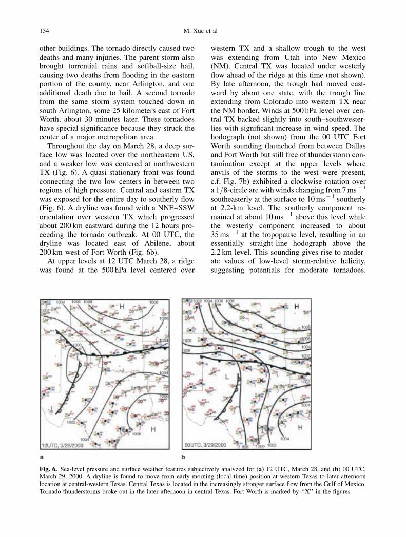
Throughout the day on March 28, a deep sur-face low was located over the northeastern US,and a weaker low was centered at northwesternTX (Fig. 6). A quasi-stationary front was foundconnecting the two low centers in between tworegions of high pressure. Central and eastern TXwas exposed for the entire day to southerly flow(Fig. 6). A dryline was found with a NNE–SSWorientation over western TX which progressedabout 200 km eastward during the 12 hours pro-ceeding the tornado outbreak. At 00 UTC, thedryline was located east of Abilene, about200 km west of Fort Worth (Fig. 6b).

At upper levels at 12 UTC March 28, a ridgewas found at the 500 hPa level centered over

western TX and a shallow trough to the westwas extending from Utah into New Mexico(NM). Central TX was located under westerlyflow ahead of the ridge at this time (not shown).By late afternoon, the trough had moved east-ward by about one state, with the trough lineextending from Colorado into western TX nearthe NM border. Winds at 500 hPa level over cen-tral TX backed slightly into south–southwester-lies with significant increase in wind speed. Thehodograph (not shown) from the 00 UTC FortWorth sounding (launched from between Dallasand Fort Worth but still free of thunderstorm con-tamination except at the upper levels whereanvils of the storms to the west were present,c.f. Fig. 7b) exhibited a clockwise rotation overa 1=8-circle arc with winds changing from 7 ms� 1

southeasterly at the surface to 10 ms� 1 southerlyat 2.2-km level. The southerly component re-mained at about 10 ms� 1 above this level whilethe westerly component increased to about35 ms� 1 at the tropopause level, resulting in anessentially straight-line hodograph above the2.2 km level. This sounding gives rise to moder-ate values of low-level storm-relative helicity,suggesting potentials for moderate tornadoes.

Fig. 6. Sea-level pressure and surface weather features subjectively analyzed for (a) 12 UTC, March 28, and (b) 00 UTC,March 29, 2000. A dryline is found to move from early morning (local time) position at western Texas to later afternoonlocation at central-western Texas. Central Texas is located in the increasingly stronger surface flow from the Gulf of Mexico.Tornado thunderstorms broke out in the later afternoon in central Texas. Fort Worth is marked by ‘‘X’’ in the figures

154 M. Xue et al

In the following, we present results from a set ofprediction experiments for this case.

4.2. Design of forecast experiments

The prediction experiments were performedusing the ARPS system. One of the goals of thiswork is to test our ability to initialize a modelwith pre-existing thunderstorms and determinis-tically predict them at fine spatial scales whenusing a state-of-the-art numerical model and itsdata assimilation system. For the latter, we areparticularly interested in the impact of cloud anal-ysis procedures in the ADAS that makes useof radar reflectivity data to initialize the watervapor, hydrometeor and temperature perturbationfields inside clouds. We also want to test theimpact of assimilating these data into the modelat a relatively high (� 15 min) frequency.

For the prediction experiments, two levels ofone-way nested grids were used, with the resolu-tions being 9 and 3 km. The two grids cover areasof 1000� 1000 and 450� 300 km2, respectively.Similar to the experiments for the Arkansas tor-nado case, full model physics were employed,including the soil model. The Lin et al’s (1983)ice microphysics scheme was used on both grids,while the Kain–Fritsch cumulus parameteriza-tion was used on the 9-km grid only. The 9-kmgrid was initialized at 18 UTC, March 28, from asingle ADAS analysis that combined rawinsonde,wind profiler, NWS surface and Oklahoma Mes-onet data and the NCEP ETA 18 UTC analysis asthe background. At the lateral boundaries, the9-km grid was forced by the ETA 18 UTC fore-casts at 3-hour intervals. No radar or data assim-ilation was performed on the 9-km grid. Theforecast was run for 12 hours, ending at 06UTC, March 29. With the primary goal of ini-tializing pre-existing storms, we started the3 km grid at later times, when the thunderstormshad already formed and been observed (in precip-itation mode) by the WSR-88D Doppler radars(also known as NEXRAD, Crum and Albert,1993).

Despite recent prototyping efforts in the real-time access of WSR-88D full-volume (level-II)data (Droegemeier et al, 2002), and the ability atCAPS to ingest data from several surroundingradars in real time, (including Fort Worth) formuch of the country only WSR-88D level-III

(also known as NIDS, Baer, 1991) data are avail-able in real time so far. The level-III data con-tains only the lowest four elevation scans and theradial velocities are quantized at about 5 ms� 1

intervals. Although the latter were used in theADAS to perform adjustments to the wind fields,they are not good enough for performing velocityand thermodynamics retrievals, however. Sincethe level-III data are widely available in realtime, we test our ability to most effectively usethem for initializing pre-existing storms in thiscase study.

Three forecast experiments were performed atthe 3-km resolution. The first (FCST22) startedfrom ADAS analysis at 22 UTC using the 9-km4-hour forecast as the analysis background, thelevel-III reflectivity and radial velocity data fromthe Fort Worth, TX (KFWS), Fort Hood, TX(KGRK), Dyess Air Force Base, TX (KDYX),and Fredrick, OK (KFDR) radars, and the NWSsurface observations. KGRK, KDYX and KFDRradars are located to the south–southwest, westand northwest of Fort Worth, respectively, andare about 200 km to 250 km from Fort Worth.They therefore provide a good coverage for thesource regions of storms west of Fort Worth.

The second experiment (FCST23) is initializedthe same way as FCST22, except at 23 UTC, onehour later. The third, which we will call the con-trol experiment (CNTL), employed 15-min inter-mittent assimilation cycles that started at 22 UTCand lasted for one hour. Radar and surface datawere used. The true forecast started at 23 UTCfrom the assimilated initial condition. Because ofthe non-standard initialization times, the upperlevel state relies heavily on information carriedover from 18 UTC or even earlier (through ETA)by the coarser-resolution grid. The pre-forecastperiods by the 9-km grid are generally helpfulin reducing the spin-up time on the 3-km gridfor both the assimilation and cold start runs(because FCST22 and FCST23 actually used9-km forecasts as the analysis background,‘‘warm start’’ is probably a better descriptionfor the runs).

Since the cloud analysis procedure is used, webriefly describe the package here. In order toprovide detailed initial conditions for moisturevariables in the ARPS, and to serve as the basisfor moisture data assimilation, a cloud analysisprocedure has been developed as a component of


the ADAS. The procedure is a customization ofthe algorithms used by the Forecast Systems Labin the Local Analysis and Prediction System(LAPS, Albers et al, 1996) with enhancementsand refinements (Zhang et al, 1998; Zhang,1999). It incorporates cloud reports from surfacestations reporting World Meteorological Orga-nization (WMO) standard Aviation RoutineWeather Reports (METARs), satellite infraredand visible imagery data, and radar reflectivityto construct three-dimensional cloud and precipi-tate fields. The products of the analysis packageinclude three-dimensional cloud cover, cloudliquid and ice water mixing ratios, cloud and pre-cipitate types, in-cloud vertical velocity, icingseverity index, and rain=snow=hail mixing ratios.Cloud base, top and cloud ceiling fields are alsoderived. A latent heat adjustment to temperaturebased on added adiabatic liquid water content isapplied, so that the in-cloud temperature is rea-sonably consistent with the water fields. Moredetails on the package can be found in the refer-ences quoted above.

For our experiments, satellite data were notused in our cloud analyses. This is done on pur-pose to highlight and better evaluate the impactof level-III radar data. The simple wind adjust-ment procedure using radar radial velocity data isdescribed in Brewster (1996). With the proce-dure, the radial winds are optimally combinedwith the background winds making use of theirerror characteristics information. It can be effec-tive for updating the radial wind component butis not able to recover much of the tangential windinformation.

4.3. Results of control experiment

Limited by space, we will present results fromthe 3-km grid only and we will start with controlexperiment CNTL. The predicted reflectivity(derived from hydrometeor fields in the sameway as in Sect. 3), wind and potential tempera-ture fields at the surface (actually at the first

model level which is roughly 10 m above ground)are plotted in Fig. 8 at half hour intervals for 2.5hours starting from 23:30 UTC, which is 1.5hours after the data assimilation cycle is startedand 0.5 hour after the true initial time at 23 UTC.All 3-km forecasts ended at 03 UTC, March 29.Figure 7 shows the corresponding low-levelreflectivity fields from the level-III data of theFort Worth radar. Tarrant and Dallas countiesare highlighted in the plots with darkened bor-ders. Downtown Fort Worth and Dallas are lo-cated roughly at the center of the left (Tarrant)and right (Dallas) counties, respectively.

At 23:30 UTC, two clusters of storms arefound from both the radar observation (Fig. 7a)and in the model (Fig. 8a), one near the north-west and one at the southwest corners of theplotted domain. Each of the observed clusterscontained about five reflectivity maxima, moreor less related to individual storm cells. In themodel, the cells are less distinct, which isbelieved to be due to the averaging to the rela-tively coarse 3-km resolution (improvements tothe radar remapping methods are being pursued).The most prominent features in the surface floware strong divergence from the storm downdraftsbehind the leading gust fronts and the strong con-vergence at the gust front. Localized centers ofmaximum convergence can also be found alongthe gust fronts, with the strongest one located atthe southeastern edge of the reflectivity maxi-mum in the northwest cluster, close to thewestern border of Tarrant county. In the radarobservation (Fig. 7a), a matching cell (storm A)is found located off the western border of thesame county and shows radar echoes with anappendage in the southwest flank, sometimescalled the hook precursor. It is this storm thatspawned the Fort Worth and Arlington tornadoes,about 45 min and just over an hour later, respec-tively. Another more isolated cell is found aboutone county (� 45 km) south of Tarrant county(storm B, Fig. 7a), and this cell is also repro-duced well by the model (Fig. 8a).

1

Fig. 7. Reflectivity fields based on level-III data at approximately half an hour intervals from 23:28UTC, March 28 through2:03UTC, March 29, 2000, from the lowest elevation (0.5 ) scan of the Fort Worth radar (marked as KFWS). Also shown arecounty borders. Forth Worth and Dallas are located in the highlighted Tarrant (left) and Dallas (right) counties, respectively.Major storm cells are marked by capital letters. The domain shown is 200 km on each side. The two highlighted counties areabout 50� 50 km2 in size

156 M. Xue et al


Fig. 8. Similar to Fig. 7, except that they are ground-level reflectivity fields predicted by the ARPS in the control experiment.Again major storm cells are marked by capital letters. Only the central portion of model domain is shown. The domain shownis about 200 km on each side, representing the portion of 3 km grid between 115 and 315 km in x-direction and 30 and 230 kmin y-direction

Half an hour after the analysis at 00 UTC, andabout 15 minutes before the Fort Worth tornadotouchdown, the leading storm cell with stronglow-level convergence from the northwesterncluster (storm A in Fig. 8) had moved to thewestern part of Tarrant county (Fig. 8b) in themodel. The low-level convergence is even stron-ger and is located slightly west of the countycenter, right over downtown Fort Worth. Therear-flank-downdraft (RFD) had been signifi-cantly enhanced and the gust front associatedwith RFD had turned counterclockwise into aN–S orientation. It is interesting to note that asignificant part of the temperature gradient seemsto lag behind the leading edge of the gust front,with the latter being better defined by the surfacewinds. This may be an example of strong tem-perature gradient not being associated with theleading edge of the gust front.

By 00 UTC, the forward-flank (FF) gust frontin the model had also been, as indicated by thesurface temperature contours, velocity vectorsas well as the reflectivity pattern, enhanced andhad rotated clockwise into an E–W orientation(Fig. 8b). There existed a significant componentin the surface winds that was parallel to the for-ward-flank gust-front. Clearly, all key ingredientsfound in the classical conceptual models (e.g.,Lemon and Doswell, 1979) of the low-levelstructure of tornadic thunderstorms are in placeand tornadogenesis can be expected at or near theintersecting point of the FF and RF gust fronts.Indeed, in the real world, a tornado was spawnedabout 15 minutes later, at a location that is almostexactly the same as suggested by the currentprediction.

The forecast was not perfect, however. At thelow levels, the observed radar echo is stronger onthe forward flank where the rear flank echo ishardly identifiable (Fig. 7b). The echo does exhib-it a hook shape on its western end at this time(Fig. 7b) and later (Fig. 7c). The composite (ver-tical column maximum) reflectivity plot (notshown) does show more southward extension ofecho at the western end, indicating the presenceof rear flank downdraft whose associated precip-itation had not yet reached the ground. The pre-cipitation in this area eventually did reach theground, about 40 minutes later (see Fig. 7d),creating low-level echo patterns that closelymatch the predicted ones at and after 00 UTC.

It is seen in Fig. 8 that storm B, found at 23:28UTC, propagated due east and developed anincreasingly prominent hook shape at the westernend of the echo. No information is availableas to whether it produced any tornado. It is,however, one of the strongest rotating stormsobserved in the current domain. This storm isalso reasonably well predicted by the modelexcept for certain details. Between 23:30 and00 UTC, the model storm split into two (denotedas B and B0 in Fig. 8), with the left membermoving off to the northeast while the right moverstaying its eastward course. Storm B0 eventu-ally merged with storm A (Fig. 8b–8d) whilethe right member gained rotational charac-teristics. Throughout the time, this right moverpossessed characteristics and positions (Fig.8a–8f) that closely match the observed storm B(Fig. 7a–7f).

At 00:30 UTC, some significant differencesare found between the model and observationsin SW Tarrant county and further SW of thatcounty. In the model, intense reflectivity is foundextending from storm A in the NE corner ofTarrant county through the SW corner of thecounty and reaching the SW corner of the nextcounty to the southwest. Such an echo is notfound in the actual radar data. It was found thatthis line-oriented storm was triggered when thegust front from the northwestern cluster collidedwith the outflow on the backside of storm B. Thefirst sign of storm initiation along the collisionzone can actually be seen as early as 00 UTC inFig. 8b. This storm moved east–northeastwardand also developed significant low-level rotationlater on (Fig. 8e, d). Without detailed analysis ofsurface flow, using, for example Doppler velocityand their retrievals, it is not clear if there wasactually gust front convergence in this regionand if there was, whether storm initiation wassuppressed by unfavorable environmental ther-modynamic conditions. One known fact is thatthe surface thunderstorm outflows in the modelwere rather strong, which was apparently helpedby the cloud analysis and assimilation cycles inwhich hydrometeors were added into the modelthat in turn enhanced downdrafts and cold poolsthrough evaporative cooling and water loading. Itis possible that this part is overdone in the cloudanalysis package or the analysis increments werespread over too large areas by the analysis

M. Xue et al: ARPS, storm-scale numerical weather prediction and data assimilation 159

procedure on the still rather coarse (3-km) reso-lution grid.

At 00:30 UTC, despite the interferences ofstorms B0 and C, storm A still exhibited clearhook characteristics with a strong low-level con-vergence center that is located at the border ofTarrant and Dallas counties where the secondtornado was reported at Arlington close to thistime. The evolution of storm A in the model after00:30 UTC differs from the observation, primarydue to the interferences of storms B0 and C.Storm A in the real world moved due east afterthis time into Dallas county and split into twocells after it reached the eastern part of Dallascounty (Fig. 7f). In the model, storm A weakenedafter it merged with the B0, the spuriously splitmember from original storm B. The combinedstorm moved off towards northeast. Storm Cdeveloped into a dominant cell at and after1:30 UTC (Fig. 8e, f) that processed strong rota-tional characteristics that somewhat matched thereal storm A.

Without a close look at the evolution history ofthe cells in the model, one could easily regardstorm C at 2:00 UTC as storm A that is posi-tioned half a country too far south. If, however,we take a relaxed view of cell evolution and con-sider storm C part of storm A (they were indeedconnected from the beginning), we have a singleentity that moved eastward while its southern

part became dominant. By 2:00 UTC, it reachedthe eastern border of Dallas county with south-ward position error of about half a county(� 25 km) compared with the radar observation.The storm cell that moved off to the northwestcan be instead considered storm B0 (which isin fact quite true judging from the low-levelvertical velocity fields). This view leads to a bet-ter overall agreement between the model andobservation.

The above results showed that starting from aninitial condition that assimilated radar and otherobservations over a one-hour period, the model isable to predict the timing, location and key char-acteristics of convective storms with very goodaccuracy. The correct prediction of the develop-ment of strong rotation in one of the modelstorms within tens of minutes and few kilometersof real tornado touchdowns is especially encour-aging. Our results also show that when severalstorms are spaced closely, complex storm inter-action can occur, through, for example, gust frontcollisions. Spurious cells can be triggered whensuch interactions are incorrectly or inaccuratelyhandled by the model. In the following section,we will discuss the results from two other experi-ments that did not employ a data assimilationcycle, and through the comparisons we hope togain additional insights on the impact of level-IIIradar data and of the assimilation cycle.

Fig. 9. Same as Fig. 8, except that they are predicted reflectivity fields from experiment FCST22 that started from initial anal-ysis at 22 UTC, March 28, 2000. No data assimilation cycle was employed. Two model storms cells are marked as X and Y

160 M. Xue et al

Fig. 10. Same as Fig. 9, except that they are predicted reflectivity fields from experiment FCST23 that started from initialanalysis at 23 UTC, March 28, 2000. No data assimilation cycle was employed. This run had the same initial time as thecontrol experiment shown in Fig. 8, but different initial condition


4.4. Comparison with non-cycled forecasts

The two and three-hour forecast fields fromFCST22, the forecast beginning at 22 UTC andproceeding without cycled assimilation, areshown in Fig. 9. It is clear that this forecast ismuch worse than the control. The northwest clus-ter of storms is completely missing, so is stormcell B. The main predicted features in the plotteddomain are three cells found at 00 UTC near thesouthwest corner. By 01 UTC, the two north-western cells merged together while the one atthe southern boundary split into two. They allmoved in the northeast direction. There is notmuch correspondence between the model stormswith observed ones.

The forecast fields from FCST23 correspond-ing to those in Fig. 7 are plotted in Fig. 10. Havingbeen initialized one hour later than FCST22, theresults are much better. All three areas of stormactivity are reasonably well represented at 23:30UTC, 30 min into the forecast. With a shorterspin-up time, the surface outflow and gust frontsare much weaker compared to CNTL. In fact, sur-face divergence inside the cold pool was stillmostly missing at this time. In the model, stormA weakened as it propagated southeastward intoTarrant county before it intensified again after itsgust front collided with the outflow from alsoweakening storm B (Fig. 10c and Fig. 10d). Therotational characteristics of storm A are evidentbut weaker than in CNTL and remained so forthe rest of its life. The gust front collision alsoenhanced the southwestern part of storm A, andcreated a connected cell we call storm C. Storm Bdid not produce a split cell as in CNTL, but itweakened significantly and later merged withcells behind it. It is clear that the results from thisrun, which lacked an assimilation cycle, are not asgood, and it missed the intensification of low-level convergence and rotation associated withstorms A and B entirely. Such intensification iskey in suggesting the high tornadogenesis poten-tial with these storms.

4.5. Discussion

From the results of the three experiments thatused level-III data in different ways, it is clearthat the assimilation of the data had a significantpositive impact on the forecast. The cloud analy-sis helped to pinpoint the location of initial storm

cells and built a reasonably correct cloud struc-ture that went on to produce the downdraft andcold pools in support of the subsequent develop-ment and evolution. The prediction of storm cellspossessing strong low-level rotations at timesvery close to the observed times and locationsof tornado touchdowns and of the low-level vor-tex signatures that match radar observations isespecially encouraging. We plan to further ana-lyze the data to better understand the dynamicalprocesses involved. We also plan to apply ourvelocity and thermodynamic retrieval schemesto this case using full volume level-II data andfurther examine the impact of retrieved veloc-ity and thermodynamic fields on the modelprediction.

5. The ARPS 3DVAR system

5.1. Introduction

For the previous two case studies, the ADASsystem was used for data analysis. The ADASsystem is based on the Bratseth (1986) successivecorrection scheme. It is flexible in dealing withdata of varying spatial densities and is com-putationally very efficient. A drawback of theBratseth scheme, like any other non-variationalscheme including the popular optimal interpola-tion (OI) (Bratseth scheme actually converges toOI), is that observed quantities different from theanalysis variables cannot be directly analyzed.Examples of such observations include precipita-ble water from GPS, satellite radiances, and radarradial velocity and reflectivity. Variational meth-ods have the advantages of being able to directlyuse the observations in a cost function, andthrough the minimization of this function, thedesired analysis variables are obtained that givea best fit to the data, subjecting to backgroundand other dynamic constraints (see, e.g., discus-sions in Courtier et al, 1998).

While four-dimensional variational (4DVAR)data assimilation is generally considered superiorand considerable successes have been achievedin applying 4DVAR to operational systems(e.g., Rabier et al, 2000) and to small-scale appli-cations with radar data (e.g., Sun and Crook,2001; Gao et al, 1998), 4DVAR is computation-ally expensive. Furthermore, a three-dimensionalvariational (3DVAR) assimilation system is the

162 M. Xue et al

necessary first, and also computationally moreefficient, step towards that the eventual goal ofdoing 4DVAR data assimilation. In this section,we describe the preliminary version of an incre-mental 3DVAR system developed recently atCAPS. An analysis example will also be given.

5.2. 3DVAR formulation

Following standard practice, we first define a costfunction, J, as

JðxÞ ¼ 1

2ðx � xbÞT

B�1ðx � xbÞ

þ 1

2½HðxÞ � yoTR�1½HðxÞ � yo þ Jc;

ð1Þwhere the first term, usually called the back-ground term, measures the departure of the anal-ysis vector, x, from the background, xb, which isweighted by the inverse of the background errorcovariance matrix B. In our current scheme, theanalysis vector x contains the three windcomponents (u, v, and w), potential temperature,�, pressure, p, water vapor mixing ratio, qv, andthe mixing ratios for hydrometeor species. Thesecond term, usually called the observation term,measures the departure of the analysis from theobservation vector yo. The analysis is projectedto the observation space by the forward operatorH. For a 4DVAR implementation, H also con-tains the forward prediction model. The obser-vation term is weighted by the inverse of thecombined observation and observation-operatorerror covariance matrix R. In an assimilation sys-tem, the background is usually a forecast validat the analysis time. Observations that havebeen tested with the system include single-levelsurface data (including Oklahoma Mesonet),multiple-level or upper-air observations (suchas rawinsondes and wind profilers), and Dopplerradar radial velocity and reflectivity data.

In Eq. (1), Jc, represents dynamic constraints.For small-scale nonhydrostatic flows, this term isnontrivial because simple large-scale (e.g., geo-strophic) balances are generally invalid. Foranalysis of radar data, especially of the radialvelocity, dynamic constraints, such as the 3-Dmass continuity equation and 3-D diagnosticpressure equation, are usually required. An initialversion of this component, which includes mass

continuity as a weak constraint and the diagnos-tic pressure equation as a strong constraint, hasbeen implemented, refinement and testing of theprocedure are underway. Here, we will discussthe background and observational terms only.

The 3DVAR analysis determines the modelstate, x, for which J is a minimum. This occurswhen the derivatives of J with respect to allcontrol variables vanish. To avoid the computa-tionally overwhelming problem of inverting thecovariance matrix B in the minimization of J,and to improve the conditioning of the minimiza-tion problem, we perform, following Lorenc(1997), a transformation of control variables,from x to v, according to

ffiffiffiffi

Bp

v ¼ ðx � xbÞ ¼�x. This leads to a new representation of the costfunction in incremental form:

Jinc ¼1

2vTv þ 1

2ðH

ffiffiffiffi

Bp

v � dÞTR�1ðHffiffiffiffi

Bp

v � dÞ

þ Jc; ð2Þ

where H is the linearized version of H andd� yo�H(xb). With this cost function, no inver-sion of B is necessary as long as we start from azero initial guess of v, a common and preferredpractice. Once v is obtained, x can be obtainedby applying

ffiffiffiffi

Bp

to v.To avoid explicitly storing and applying the

matrixffiffiffiffi

Bp

, spatial filters have been proposedto model its effect. Gaussian-type filters wereused by Daley (1991) and Huang (2001), forexample. In our system, we choose the class ofrecursive spatial filters first proposed by Purserand McQuiqq (1982) and extended by Purseret al (2001). The filter requires no extra storageand is computationally very efficient. It asymp-totically approaches the Gaussian filter when thenumber of applications goes to infinity. Evenwith only a few applications, the approximationcan be rather good, especially if a high-orderfilter is used.

To use the filter, the matrixffiffiffiffi

Bp

is rewritten asffiffiffiffi

Bp

¼ DF where D is a diagonal matrix consist-ing of the standard deviation of backgrounderrors, or, the square root of the error variances.F is modeled by a recursive filter, which, whenusing first order, is defined by

bi ¼ �bi�1 þ ð1 � �Þai for i ¼ 1; . . . ; n;

ci ¼ �ciþ1 þ ð1 � �Þbi for i ¼ n; . . . ; 1; ð3Þ


where ai is the initial value at grid point i, bi isthe intermediate value after a swap from i¼ 1 ton, is performed, and ci is the final value after thefiltering. � is the filter coefficient. Typically, theabove algorithm is applied in all coordinatedirections in succession, and the filter is appliedmultiple times to achieve the desired effect.

With the current implementation and thechoice of primitive model variables u, v, w, �,p, qv and the hydrometeor species as control vari-ables, we are not including in the backgroundterm cross-correlations between variables. Thecross-correlation can be and is, however, realizedthrough the dynamic constraints, i.e., the Jc term,in (1), but clearly those relying on quasi-geo-strophic balance are not appropriate at thenonhydrostatic scale. With several existing oper-ational 3DVAR systems (e.g., Lorenc, 1997), thecross-correlation is partially realized by choosingstreamfunction and velocity potential as the con-trol variables. The effectiveness of this approachremains to be investigated at the small scales.

In our current system, we assume that theobservation errors are independent, that is, theobservation error covariance matrix, R, is a diag-onal matrix, and the diagonal elements are spec-ified according to the estimated errors of theobservations. This assumption is not as bad asit sounds when proper steps including bias cor-rection are taken (Purser and Derber, 2001).

5.3. Example 3DVAR analysis

As a demonstration, the case of June 8, 1995 isused to test the 3DVAR scheme. It was a majorday during the 1995 Verification on Onset ofRotation in Tornadoes Experiment (VORTEX95) as several damaging tornadoes were pro-duced by storms in the eastern Texas Panhandle.The case has been studied by Brewster (2002b).Our analyses were performed on a 73� 73� 43grid with a 12 km horizontal grid spacing.

During the analysis, the change in the costfunction and the norm of its gradient are moni-tored. It was found that the cost function plottedas a function of the number of iterations startedto level off after 10 and became essentially flatafter 20 iterations (not shown). The decrease inthe norm of the gradient continued until 50 itera-tions, however. Fifty iterations were used for theresults presented here.

To show that the current 3DVAR system pro-duces reasonable analysis, we compare the resultswith the ADAS analysis. The ADAS analysis wasobtained using four correction passes with thehorizontal correlation scaling parameter fixed at50 km for all passes to facilitate easy comparisonwith the 3DVAR analysis. The 50 km scale waschosen to match roughly the average station den-sity of the surface data, standard airways observa-tions and Oklahoma Mesonet data, the primarysource of data in this case. For the 3DVAR anal-ysis, horizontally homogeneous and isotropic fil-ter scale that is expected to yield a similarhorizontal influence range as that in ADAS wasused. In Fig. 11, we show the contours of east-west velocity and wind vectors at the surfaceand in Fig. 12 the surface potential temperatureand wind vectors. Observations at the surface sta-tions are overlaid. Comparing the 3DVAR withthe ADAS and with the observations, we cansee that the two analyses are comparable in qual-ity and due to the relatively small influence rangeor filter scale, the analyses have a tight fit with theobservations and at the same time show localizedanalysis increments surrounding isolated observa-tions. In the ADAS, the inhomogeneous stationdensity is handled by using different influenceranges for different observational networks inthe multiple analysis passes, and with 3DVAR,this effect can be achieved by either using spa-tially inhomogeneous filter scales and=or a simi-lar multi-pass strategy. We note that it is not ourpurpose here to show that one is superior to theother when we compare the 3DVAR analysis tothat of ADAS. In fact, with the Bratseth schemebeing able to converge to an OI scheme (Bratseth,1986; see also Daley, 1991) which in turn can bemade equivalent to a 3DVAR when only conven-tional data are involved (see, e.g., Courtier, 1997),it is possible to configure the 3DVAR to producevery similar results as the ADAS for this demon-stration. The full advantages of 3DVAR schemeswill not be realized until indirect observations areinvolved and when proper estimates of the back-ground and observational error correlations areused.

Standard single-observation experiments havealso been performed which confirmed that therecursive filter produces the desired spread ofthe observational increments. The strength ofits effect depends on the number of filter passes

164 M. Xue et al

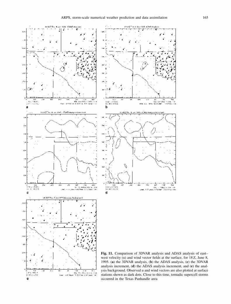
Fig. 11. Comparison of 3DVAR analysis and ADAS analysis of east–west velocity (u) and wind vector fields at the surface, for 18 Z, June 8,1995. (a) the 3DVAR analysis, (b) the ADAS analysis, (c) the 3DVARanalysis increment, (d) the ADAS analysis increment, and (e) the anal-ysis background. Observed u and wind vectors are also plotted at surfacestations shown as dark dots. Close to this time, tornadic supercell stormsoccurred in the Texas Panhandle area


Fig. 12. As Fig. 11, but the contours are for potential temperature

166 M. Xue et al

used and on the correlation scale chosen. It isverified that the isotropic spread of the observa-tion information when using a single pass of thefilter agrees with theoretical estimate. As with allvariational data assimilation system, careful tun-ing and refinement are still needed, and the truetest of the analysis quality will be the quality offorecast resulting from the analysis.

Considering that weather features at the non-hydrostatic scales are often highly intermittent inboth space and time and such flows tend to havemuch shorter lifetimes than those for which tra-ditional 3DVAR techniques were designed for,much work is still needed in determining flowdependent, three-dimensional and anisotropicbackground error correlations and the filterscales, and in applying dynamics constraints suit-able for flows at such scales. These are topics forcontinued research.

6. Summary

In this paper, we first described the current statusof the Advanced Regional Prediction System ofthe Center for Analysis and Prediction of Stormsat the University of Oklahoma. A brief outline offuture plans was also given. Two rather successfulcases of explicit prediction of tornadic thunder-storms were then shown. In the first case, a seriesof supercell storms that produced a historicalnumber of tornadoes was successfully predictedmore than 8 hours in advance. The storms agreedwith observed storms to within tens of kilometersin space with initiation timing errors of less than 2hours. The general behavior and evolution of pre-dicted thunderstorms agreed very well with radarobservations. In the second case, radar reflectivityand radial velocity were assimilated into themodel at 15-minute intervals and the ensuingforecast for several hours accurately reproducedthe intensification and evolution of an actual tor-nadic supercell that spawned two tornadoes over amajor metropolitan area. These results make usoptimistic about being able to deterministicallypredict severe convective events as such with sig-nificant lead time. To complete the paper, webriefly described a recently developed 3DVARsystem in the ARPS framework. Our goal is tocombine several steps of Doppler radar retrievalwith the analysis of other data types into a singlevariational framework and eventually include the

ARPS adjoint to establish a true four-dimensionalvariational data assimilation system. The latterdevelopmental work will also directly contributeto the 3DVAR system of the new U.S. WeatherResearch and Forecast (WRF) model under devel-opment. We are especially pleased that the goalsand development strategies for the WRF modelare very similar to those of the ARPS about 10years ago. This not only affirms the validity of thedirection taken by CAPS, but also demonstratesthe value of building upon past experience totransform research into operations.

Acknowledgment

This research was supported by NSF ATM92-20009, ATM99-09007, NOAA NA67RJ0150 and a grant from FAA.D. H. Wang was partially supported by a research contractfrom Weather Decision Technology, Inc. Jason Levit isthanked for assistance handling WRS-88D tape data. Manyother CAPS scientists contributed to the ARPS systemtesting and development. Most of the plots in the paperwere generated by programs based on the ZXPLOTgraphics package developed by the first author and ZuojunZhang. Computations of the Arkansas tornado case werecompleted on National Center for Supercomputing Appli-cation’s SGI Origin 2000 array.

References

Albers SC, McGinley JA, Birkenheuer DA, Smart JR (1996)The local analysis and prediction system (LAPS): Anal-ysis of clouds, precipitation and temperature. Wea Fore-cast 11: 273–287

Baer VE (1991) The transition from the present radardissimilation system to the NEXRAD Information Dis-semination Service (NIDS). Bull Amer Meteor Soc 72:29–33

Bischof C, Carle A, Corliss G, Griewank A, Hovland P(1992) ADIFOR – generating derivative codes from For-tran programs. Sci Progr 1: 11–29

Bratseth AM (1986) Statistical interpolation by means ofsuccessive corrections. Tellus 38A: 439–447

Brewster K (1996) Application of a Bratseth analysis schemeincluding Doppler radar data. Preprints, 15th Conf.Wea. Anal. Forecast. Amer. Meteor. Soc., Norfolk, VA,pp 92–95

Brewster K (1999) Phase-correction data assimilation andapplication to storm-scale numerical weather prediction.Ph.D. Diss., University of Oklahoma, Norman, OK

Brewster KA (2002a) Phase-correcting data assimilation andapplication to storm scale numerical weather prediction.Part I: Method description and simulation testing. MonWea Rev (accepted)

Brewster KA (2002b) Phase-correcting data assimilationand application to storm scale numerical weather predic-tion. Part II: Application to a severe storm outreak. MonWea Rev (accepted)


CAPS (1992) ARPS Version 3.0 User’s Guide. Availablefrom Center for Analysis and Prediction of Storms, Uni-versity of Oklahoma, Norman OK 73019, 183 pp

Carpenter RLJ, Droegemeier KK, Bassett GM, WeygandtSS, Jahn DE, Stevenson S, Qualley W, Strasser R (1999)Storm-scale numerical weather prediction for commercialand military aviation, Part I: Results from operationaltests in 1998. Preprints, 8th Conf. on Aviation, Range,and Aerospace Meteor. Amer. Meteor. Soc., Dallas,TX

Chou M-D (1990) Parameterization for the absorption ofsolar radiation by O2 and CO2 with application to climatestudies. J Clim 3: 209–217

Chou M-D (1992) A solar radiation model for climatestudies. J Atmos Sci 49: 762–772

Chou M-D, Suarez MJ (1994) An efficient thermal infraredradiation parameterization for use in general circulationmodels, NASA Tech. Memo. 104606, 85 pp. [Availablefrom NASA Center for Aerospace Information, 800Elkridge Landing Road, Linthicum Heights, MD21090-2934.]

Courtier P (1997) Variational methods. J Meteor Soc Japan75: 211–218

Courtier P, Andersson E, Keckley E, Pailleux J, Vasiljevic D,Hamurd M, Hollingsworth A, Rabier F, Fisher M (1998)The ECMWF implementation of three-dimensional var-iational assimilation (3D-Var). I: Formulation. Quart JRoy Meteor Soc 124: 1783–1808

Crum TD, Albert RL (1993) The WSR-88D and the WSR-88D operational support facility. Bull Amer Meteor Soc74: 1669–1687

Daley R (1991) Atmospheric data analysis. CambridgeUniversity Press, 457 pp

Droegemeier KK (1990) Toward a science of storm-scale prediction. Preprint, 16th Conf. on Severe LocalStorms. Amer. Meteor. Soc., Kananaskis Park, Alberta,Canada

Droegemeier KK (1997) The numerical prediction of thun-derstorms: Challenges, potential benefits, and results fromreal time operational tests. WMO Bull 46: 324–336

Droegemeier KK, Kelleher K, Crum TD, Levit JJ, GrecoSAD, Miller L, Sinclair C, Benner M, Fulker DW, EdmonH (2002) Project CRAFT: A test bed for demonstratingthe real time acquisition and archival of WSR-88D base(level II) data. Preprint, 18th Int. Conf. IIPS Meteor.Ocean. Hydrology. Amer. Meteor. Soc., Orlando, FL

Droegemeier KK, Xue M, Brewster K, Liu Y, Park S, Carr F,Mewes J, Zong J, Sathye A, Bassett G, Zou M, CarpenterR, McCarthy D, Andra D, Janish P, Graham R, SanielviciS, Brown J, Loftis B, McLain K (1996) The 1996 CAPSspring operational forecasting period: Realtime storm-scale NWP, Part I: Goals and methodology. Preprints,11th Conf. on Num. Wea. Pred. Amer. Meteor. Soc.,Norfolk, VA

Droegemeier KK, Xue M, Johnson K, O’Keefe M, SawdeyA, Sabot G, Wholey S, Mills K (1995) Design andimplementation of a scalable-parallel stormscale numer-ical weather prediction model. In: High PerformanceComputing (Sabot GW, ed). Reading, Mass.: Addison-Wesley, pp 45–92

Ebisuszki W, Kalnay E (1991) Ensemble experiments witha new lagged analysis forecasting scheme. 6.31–6.32,Research Activities in Atmospheric and Oceanic Model-ing Rep. 15, World Meteor. Org.

Gao J, Xue M, Brewster K, Carr F, Droegemeier KK (2001a)A three-dimensional variational data assimilation schemefor storm-scale models. Preprints, 14th Conf. on Num.Wea. Pred. Amer. Meteor. Soc., Ft. Lauderdale, FL

Gao J, Xue M, Droegemeier KK, Shapiro A (2001b) A 3-Dvariational method for single-Doppler velocity retrievalapplied to a supercell storm case. Preprints, 30th Int. Conf.Radar Meteor. Amer. Meteor. Soc., Munich, Germany

Gao J, Xue M, Shapiro A, Xu Q, Droegemeier KK (2001c)Three-dimensional simple adjoint velocity retrievals fromsingle Doppler radar. J Atmos Ocean Tech 18: 26–38

Gao J, Xue M, Wang Z, Droegemeier KK (1998) The initialcondition and explicit prediction of convection usingARPS adjoint and other retrievals methods with WSR-88D data. 12th Conf. Num. Wea. Pred. Amer. Meteor.Soc., Phoenix, AZ

Gao JD, Xue M, Shapiro A, Droegemeier KK (1999) Avariational method for the analysis of three-dimensionalwind fields from two Doppler radars. Mon Wea Rev 127:2128–2142

Hou D, Kalnay E, Droegemeier KK (2001) Objective ver-ification of the SAMEX ’98 ensemble forecasts. Mon WeaRev 129: 73–91

Huang X-Y (2001) Variational analysis using spatial filters.Mon Wea Rev 128: 2588–2600

Johnson KW, Bauer J, Riccardi GA, Droegemeier KK, XueM (1994) Distributed processing of a regional predictionmodel. Mon Wea Rev 122: 2558–2572

Kain JS, Fritsch JM (1993) Convective parameterization formesoscale models: The Kain–Fritsch scheme, The Repre-sentation of Cumulus Convection in Numerical Models,Meteor. Monogr. Amer. Meteor. Soc., pp 165–170

Kapitza H (1991) Numerical experiments with the adjoint ofa non-hydrostatic mesoscale model. Mon Wea Rev 119:2993–3011

Lafore JP, Stein J, Asencio N, Bougeault P, Ducrocq V,Duron J, Fisher C, P�eereil P, Mascart P, Masson V, Pinty JP,Redelsperger JL, Richard E, Vil�aa-Guerau de Arellano J(1998) The meso-NH atmospheric simulation system. PartI: Adiabatic formulation and control simulation. AnnGeophys 16: 90–109

Lemon LR, Doswell CA (1979) Severe thunderstorm evolu-tion and mesocyclone structure as related to tornadogen-esis. Mon Wea Rev 107: 1184–1197

Lilly DK (1990) Numerical prediction of thunderstorms –Has its time come? Quart J Roy Meteor Soc 116: 779–798

Lin Y-L, Farley RD, Orville HD (1983) Bulk parameteriza-tion of the snow field in a cloud model. J Clim ApplMeteor 22: 1065–1092

Lorenc AC (1997) Development of an operational varia-tional assimilation scheme. J Met Soc Japan 75: 339–346

Purser JR, Derber JC (2001) Unified treatment of measure-ment bias and correlation in variational analysis withconsideration of the preconditioning problem. Preprints,14th Conf. Num. Wea. Pred. Amer. Meteor. Soc., FortLauderdale, FL, pp 497–470

168 M. Xue et al

Purser RJ, Derber JC, Parrish DF, Roberts NM (2001)Numerical aspects of the application of recursive filtersto variational statistical analysis with spatially inhomo-geneous covariance. NOAA=NCEP Office Note 431,34 pp

Purser RJ, McQuiqq R (1982) A successive correctionanalysis scheme using recursive numerical filters. Met.O 11 Tech. Note, No. 154, British Meteorological Office,17 pp

Rabier F, Jarvinen H, Klinker E, Mahfouf J-F, Simmons A(2000) The ECMWF operational implementation of four-dimensional variational assimilation. I: Experimentalresults with simplified physics. Quart J Roy Met Soc126: 1143–1170

Rogers RR, Yau MK (1989) A short course in cloud physics.Pergamon Press, Oxford, 293 pp

Schultz P (1995) An explicit cloud physics parameterizationfor operational numerical weather prediction. Mon WeaRev 123: 3331–3343

Shapiro A, Droegemeier KK, Lazarus S, Weygandt S(1995a) Forward variational four-dimensional data assim-ilation and prediction experiments using a storm-scalenumerical model. Proc., Int. Symp. on Assim. Obs.Meteor. and Oceanography. World Meteor. Org., Tokyo,Japan, pp 361–366

Shapiro A, Ellis S, Shaw J (1995b) Single-Doppler radarretrievals with Phoenix II data: Clear air and microburstwind retrievals in the planetary boundary layer. J AtmosSci 52: 1265–1287

ShapiroA,RobinsonP,LevertC,GaoJ(1999)Single-Dopplervelocity retrieval experiments with a simple 4DVAR tech-nique. Preprints, 29th Int. Conf. Radar Meteor. Amer.Metero. Soc., Montreal, PQ, Canada, pp 26–29

Shapiro A, Zhao L, Zhang J, Tuttle J, Laroche S, Zawadzki I,Xu Q, Gao J (1996) Single-Doppler velocity retrievalswith hailstorm data from the North Dakota thunderstormproject. Preprints, Severe Storm Conf. Amer. Meteor.Soc., San Francisco, CA, pp 546–550

Shin K-S, Chung S-K, Lee S-Y, Yoo H-D, Lee D-I,Xue M, Brewster K, Bassett G, Park S-K, DroegemeierKK (1998) Explicit realtime operational prediction ofdeep convection over Korea. Preprints, 16th Conf. onWea. Anal. Forecasting. Amer. Meteor. Soc., Phoenix,AZ, pp 135–137

Skamarock WC, Klemp JB (1993) Adaptive grid refinementfor two-dimensional and three-dimensional nonhydro-static atmospheric flow. Mon Wea Rev 121: 788–804

Sun J, Crook NA (2001) Real-time low-level wind andtemperature analysis using single WSR-88D data. WeaForecast 16: 117–132

Sun J, Flicker DW, Lilly DK (1991) Recovery of three-dimensional wind and temperature fields from simulatedsingle-Doppler radar data. J Atmos Sci 48: 876–890

Talagrand O (1991) The use of adjoint equations in numer-ical modeling of atmospheric circulation. Automatic dif-ferentiation of algorithms: Theory, implementation, andapplication. Prec. of the first SIAM workshop on auto-matic differentiation, Brechenridge, CO, pp 169–180

Tao W-K, Simpson J, McCumber M (1989) An ice-watersaturation adjustment. Mon Wea Rev 117: 231–235

Wang Z, Droegemeier KK, White L, Navon IM (1997)Application of a New Adjoint Newton Algorithm to the3D ARPS Storm-Scale Model Using Simulated Data.Mon Wea Rev 125: 2460–2478

Wang Z, Droegemeier KK, Xue M, Park SK (1995) Sensi-tivity analysis of a 3-D compressible storm-scale model toinput parameters. Proc., Int. Symp. on Assim. Obs.Meteor. Oceanography. World Meteor. Org., Tokyo,Japan, pp 437–442

Weygandt S, Shapiro A, Droegemeier K (1998) The useof wind and thermodynamic retrievals to create initialforecast fields from single-Doppler observations of asupercell thunderstorm. Preprints, 11th Conf. on Wea.Anal. and For. Amer. Meteor. Soc., Phoenix, AZ,pp 286–288

Xue M (2000) High-order monotonic numerical diffusionand smoothing. Mon Wea Rev 128: 2853–2864

Xue M, Brewster K, Droegemeier KK, Wong V, Wang DH,Carr F, Shapiro A, Zhao LM, Weygandt S, Andra D,Janish P (1996a) The 1996 CAPS spring operationalforecasting period: Realtime storm-scale NWP, Part II:Operational summary and examples. Preprint, 11th Conf.on Num. Wea. Pred. Amer. Meteor. Soc., Norfolk, VA,pp 297–300

Xue M, Droegemeier KK, Wong V (2000) The AdvancedRegional Prediction System (ARPS) – A multiscale non-hydrostatic atmospheric simulation and prediction tool.Part I: Model dynamics and verification. Meteor AtmosPhysics 75: 161–193

Xue M, Droegemeier KK, Wong V, Shapiro A, Brewster K(1995) ARPS Version 4.0 User’s Guide. [Available fromCenter for Analysis and Prediction of Storms, Universityof Oklahoma, 100 E. Boyd St., Norman OK 73019],380 pp

Xue M, Droegemeier KK, Wong V, Shapiro A, Brewster K,Carr F, Weber D, Liu Y, Wang D-H (2001) The AdvancedRegional Prediction System (ARPS) – A multiscale non-hydrostatic atmospheric simulation and prediction tool.Part II: Model physics and applications. Meteor AtmosPhysics 76: 143–165

Xue M, Droegemeier KK, Woodward PR (1993) Simulationof tornado vortices within a supercell storm using adap-tive grid refinement technique. Preprints, 17th Conf. onSevere Local Storms, St. Louis, MO. Amer. Meteor. Soc.,pp 362–365

Xue M, Hou D-C, Wang D-H, Droegemeier KK (1998)Analysis and prediction of convective initiation along adryline. 16th Conf. Wea. Anal. Forecasting. Amer.Meteor. Soc., Phoenix, AZ, pp 161–163

Xue M, Lin S-J (2001) Numerical equivalence of advectionin flux and advective forms and quadratically conserva-tive high-order advection schemes. Mon Wea Rev 129:561–565

Xue M, Zong J, Droegemeier KK (1996b) Parameterizationof PBL turbulence in a multi-scale non-hydrostatic model.Preprint, 11th AMS Conf. Num. Wea. Pred. Amer.Metero. Soc., Norfolk, VA, pp 363–365

Zalesak ST (1979) Fully multidimensional flux-correctedtransport algorithms for fluids. J Comput Phys 31:335–362


Zhang J (1999) Moisture and Diabatic Initialization Based onRadar and Satellite Observation. PhD Thesis, University ofOklahoma, [Available from School of Meteorology, Uni-versity of Oklahoma, Norman OK 73019], 194 pp

Zhang J, Carr F (1998) Moisture and latent heating rateretrieval from radar data. Preprints, 12th Conf. on Numer-ical Weather Prediction. Amer. Meteor. Soc., Phoenix,AZ, pp 205–208

Zhang J, Carr F, Brewster K (1998) ADAS cloud analysis.Preprints, 12th Conf. on Num. Wea. Pred. Amer. Met.Soc., Phoenix, AZ, pp 185–188

Corresponding author’s address: Dr. Ming Xue, School ofMeteorology, University of Oklahoma, 100 East Boyd,Norman, OK 73019, USA (E-mail: [email protected])

170 M. Xue et al: ARPS, storm-scale numerical weather prediction and data assimilation

Documents

The Advanced Regional Prediction System (ARPS), …kkd.ou.edu/ARPSPaperIII.pdfAdvanced Regional Prediction System of the Center for Analysis and Prediction of Storms at the University