THE ACCOUNTING REVIEW pp. 27–64 Earnings …haas.berkeley.edu/faculty/papers/fan_IPO.pdf · 27 THE ACCOUNTING REVIEW Vol. 82, No. 1 2007 pp. 27–64 Earnings Management and Ownership

27

THE ACCOUNTING REVIEWVol. 82, No. 12007pp. 27–64

Earnings Management and OwnershipRetention for Initial Public Offering

Firms: Theory and EvidenceQintao Fan

University of California, Berkeley

ABSTRACT: This paper investigates, both theoretically and empirically, how earningsmanagement and ownership retention interact, and how these two jointly affect theequilibrium market valuation of IPO firms in the presence of information asymmetry.Analytically, this paper extends the univariate signaling framework of Leland and Pyle(1977) and derives an efficient signaling equilibrium in which both reported earningsand ownership retention are endogenously chosen to convey the IPO issuer’s privateinformation. It is shown that even though either ownership retention or reported earn-ings communicates the issuer’s type to the market unambiguously, the issuer will stra-tegically employ both signals to achieve separation from potential lower quality imita-tors at minimal cost. Comparative statics analysis shows that the trade-off betweenthe two signals depends critically on the uncertainty over future earnings. The theo-retical analysis generates several empirical implications regarding market efficiency, IPOpricing, and the strategic choice of earnings management. Through systematic econ-ometric analysis, I confirm the major predictions of the model.

Keywords: IPO; earnings management; information asymmetry; discretionary accruals.

Data Availability: The data used in this study are publicly available from the sourcesdescribed in the text.

I. INTRODUCTION

This paper examines, both theoretically and empirically, how earnings managementand ownership retention interact, and how these two jointly affect the equilibriumvaluation of IPO firms when there is information asymmetry between the IPO issuer

and perfectly rational investors. By earnings management, I refer to firms’ inflating reportedearnings by (1) the use of the flexibility allowed in the Generally Accepted AccountingPrinciples (GAAP) to change reported earnings without changing the underlying cash flows,

This paper is based on my dissertation completed at Stanford University. I am indebted to my committee members,Ron Kasznik, Maureen McNichols (co-chair), and Stefan Reichelstein (co-chair) for their guidance and encour-agement. Special thanks are also due to Madhav Rajan (editor) and two anonymous referees for their constructivecomments. Other helpful suggestions were provided by Sunil Dutta, George Foster, Zvi Singer, Xiao-jun Zhang,Jeffrey Zwiebel, and workshop participants at Columbia University, New York University, Northwestern University,Stanford University, University of California, Berkeley, and University of California, Riverside.

Editor’s note: This paper was accepted by Madhav Rajan.Submitted July 2005Accepted June 2006

28 Fan

The Accounting Review, January 2007

which could be labeled as misreporting, and/or (2) constructing economic events to changethe underlying cash flows itself, which could be labeled as real earnings management.1

I first show that income-increasing earnings management can prevail as the outcomeof a fully separating signaling equilibrium when an IPO issuer wants to overstate earningsto a certain level to deter a lower type from mimicking his earnings report. To the extentthat earnings management is value-detrimental to the firm, the amount of earnings man-agement necessary to achieve differentiation decreases with the level of ownership retainedby the IPO issuer. I then extend Leland and Pyle’s (1977) (hereafter, LP) univariate sig-naling model in which ownership retention is an effective signal of firm value and derivean efficient signaling equilibrium in an IPO setting in which both reported earnings andownership retention are chosen as signaling devices. As IPO issuers can signal throughboth ownership retention and reported earnings, the efficient mix must minimize total sig-naling costs. I show that, in equilibrium, many firms both over-report earnings and deviatefrom the first-best level of retained ownership. Comparative statics analysis also shows thatthe trade-off between earnings management and ownership retention depends critically onthe uncertainty over future earnings.

Prior empirical work examining earnings management behavior in the new issues mar-ket has generally focused on the notion that managers opportunistically overstate earningsto issue stocks at artificially inflated prices. As an explanation of the long-run underper-formance of IPO firms, Teoh, Welch, and Wong (1998) (hereafter, TWW) and Teoh, Wong,and Rao (1998) (hereafter, TWR) document that there is a negative correlation betweenissuing period abnormal accruals and post-issue abnormal stock returns of IPO firms, sug-gesting that investors are misled by earnings management before equity offerings and arethen disappointed as expectation errors are corrected over time. In contrast to the above‘‘managerial opportunism’’ hypothesis, I model earnings management as consequence ofthe actions of rational agents with asymmetric information, implying that, in equilibrium,investors rationally anticipate some amount of earnings management and should not besystematically fooled by the exaggerated earnings reports. Thus, on the empirical side, Ifirst reexamine the robustness of the results in TWW and TWR. Using discretionary ac-cruals estimated from cash flow statements and adjusted for a performance-matched firm’sdiscretionary accruals as suggested by Kothari et al. (2005), I find that discretionary accru-als, with or without performance matching, are the highest in the IPO year and have strongpredictive power for IPO firms’ subsequent decline in operating performance. However, inmy sample period, there is no strong evidence that discretionary accruals estimated fromcash flow statements and post-issue abnormal stock returns are negatively correlated. Per-formance matching further weakens the statistical and economic significance of the rela-tionship between the two. Taken together, the results are consistent with IPO issuers ad-vancing accruals to increase reported earnings in the issuing year, but are inconsistent withinvestors being systematically fooled by such window-dressing behavior. I then directly testthe valuation implications of my signaling model and find that both reported earnings andownership retention are strongly positively priced signals in valuing an IPO firm. Finally,employing a simultaneous equation framework to examine the joint determination of anIPO firm’s earnings management and ownership retention decisions, I find evidence that,

1 The most obvious examples of misreporting include adjusting reserves for losses such as not marking down‘‘stale’’ inventory or bad debt. As total reported earnings must equal total cash flows over the firm’s life cycle,such behavior would simply relocate an amount from one period to another. However, real earnings managementthrough changing the firm’s operations (for example, by delaying desirable investment or cutting prices to boostsales) has real consequences, and can impose significant economic costs beyond earnings reversal.

Earnings Management and Ownership Retention for Initial Public Offering Firms 29


controlling for other factors, riskier IPO firms resort more to income-increasing earningsmanagement and retain less ownership, confirming the comparative statics prediction of themodel.

An initial public offering (IPO) is the first opportunity for a firm’s founders and initialinvestors to realize the value of their ownership stake in a firm. The IPO process in theU.S. is governed by the Securities Act of 1933. A firm that decides to float a new issuehires an underwriter who performs a due-diligence investigation of the firm and then pre-pares an offering prospectus that presents externally audited financial statements for themost recent three years, along with information about the firm, its business, future prospects,competitors, and products. The prospectus is used as a marketing document by the under-writer in roadshows to solicit demand, in particular from institutional investors.

There is no doubt that IPOs are often associated with high information asymmetriesbetween insiders (entrepreneurs, management, etc.) and outside investors. Inside knowledgeconcerning investment opportunities, managerial skills, and the ability to control futureagency costs, among other things, are often the private information of management. Thisis a typical adverse selection problem and in the absence of a mechanism or institution thatwill overcome the information asymmetry, the market would fail.

LP propose a solution to this problem through a univariate signaling model with own-ership retention. They argue that when making an initial public offering, the risk-averseowner of a private firm could send a signal to the market about the value of the firm byretaining part of its equity (and thus its risk). The model yields a separating equilibriumwhere the owners of the firms of each possible value optimally retain a specific portion oftheir firm’s shares and investors correctly infer firm value from each firm’s signal.

This paper extends LP’s framework to include reported earnings as a second signal offirm value for the following reasons:

● First, when valuing an IPO firm, investors would rely heavily on financial statementsfor valuation, relative to established firms with alternative sources of information.Underwriters often set the offer price using the price-earnings multiple of a publiclytraded firm in the same industry as the prospective IPO. Thus, the IPO issuer has astrong incentive to report favorable accounting information in the prospectus to in-fluence investors’ perception of the firm’s value.

● Second, IPO issuers have considerable discretion in reporting earnings. Even thoughthe accounting reports in the offering prospectuses are required to be audited byexternal auditors to verify compliance with GAAP, the accrual accounting systempermits considerable discretion in recognizing the timing and amounts of revenuesand expenses. It is also hard for investors to judge the appropriateness of the reportedaccounting numbers due to the lack of other sources of corroborative information.Further, current accounting regulation (APB No. 20) allows IPO firms to changetheir accounting choices via retroactive restatement for all the financial statementspresented in the offerings prospectus. Thus, during the IPO process, the issuer hasexceptional opportunity to boost reported earnings.

● Third, and perhaps most important, income-increasing earnings management is ar-guably costly to the firm. Even though the manager might inflate reported earningsin a single period, over the firm’s life cycle, total reported earnings must equal totalcash flows. Thus, as accounting accruals eventually reverse, future earnings sufferfrom past manipulation, potentially triggering litigation and increases in the cost ofcapital. Further, some earnings management techniques have real economic costs,such as poor timing of sales and early liquidation of assets that are not ‘‘mature’’

30 Fan


for liquidation yet. All these costs are likely to increase with the magnitude ofearnings manipulation. In this paper, I argue that the existence of such costs preventsearnings from being inflated to the point of uninformativeness. Due to informationasymmetry surrounding an IPO, a low-quality firm has a natural tendency to over-state earnings so that it can be pooled with high-quality firms. Thus, to achieveseparation, high-quality firms have an incentive to overstate earnings to a level thatis prohibitively costly for a lower type to mimic. In equilibrium, rational investorsrealize that only a high-value firm could bear the cost of overstating earnings tosuch a high level and value the firm accordingly. In this sense, positive earningsmanagement can be viewed as a signaling device to achieve separation.

An important question in any signaling model is whether the signal being examinedwould still be used if the firm had a portfolio of signals available. Most signaling modelsexamine in isolation a somewhat arbitrary action by corporate insiders, showing that it hasthe required cost structure as in Spence (1973) or Riley (1975) for the existence of aninformation equilibrium. However, there seems to be little or no reason why firms wouldnot use a mix of variables to signal firm value. Milgrom and Roberts (1986) are the firstto study such a scenario in which a monopolist chooses advertising and price to signal hisproduct quality at least cost. Engers (1987) argues that when multiple signals are used, thedirectional impacts of individual signals might be intertwined and the mix of signalingefforts will depend upon the relative power and costs of various signals available.2 Thisstudy seeks to investigate how an IPO issuer can communicate private information to pro-spective investors at minimal cost by combining earnings management and ownership re-tention. It takes into account the interaction between the two signals and also addresses theefficiency of the two signals used. Characterization and comparative statics analysis of theresulting Pareto-dominant or efficient signaling equilibrium forms the basis of several em-pirical predictions.

Several papers have extended the basic framework of LP to examine other phenomenaobserved around initial public offerings. Hughes (1986) and Grinblatt and Hwang (1989)study the problem of IPO issuers trying to signal to investors both the mean and varianceof the firm’s future cash flows. Another signal, in addition to ownership retention, is neededto effectively communicate these two pieces of information. Hughes (1986) constructs aseparating equilibrium in which an IPO issuer uses direct disclosure to disclose the expectedvalue of the firm and uses ownership retention to signal the costs of such disclosure. InGrinblatt and Hwang (1989), the two signals are ownership retention and underpricing.3

Datar et al. (1991) examine how the choice of auditor can be used together with ownershipretention to communicate the issuer’s private information to the market. The authors showthat there exists a unique, stable separating equilibrium where each type of entrepreneurfirst separates himself from some of the other types by the quality of the auditor hired andthe resulting audited report, and then from the remaining types through ownership retention.

This paper investigates features of the IPO issuer’s cost-minimizing signaling portfolio,which involves combining earnings management and ownership retention. An interesting

2 For other papers that study an efficient signaling equilibrium with multiple signals, see John and Mishra (1990)and Viswanathan (1987).

3 Grinblatt and Hwang (1989) also assume that the firm makes a second, seasoned offering soon after the IPO,with some possibility that the firm’s type is exogenously revealed between the initial and seasoned offerings.



conclusion is that the high-type issuer actually values income-increasing earnings manage-ment as a signaling device, in addition to ownership retention.4 Further, the model’s simpleyet intuitive framework permits derivation of several empirical implications regarding mar-ket efficiency, IPO pricing, and the strategic choice of earnings management, all of whichcan be easily taken to the data and tested on observable variables.5 Through systematiceconometric analysis, I confirm the major predictions of the model.

The remainder of the paper is organized as follows. Section II describes the setting ofthe model and its underlying assumptions. Section III discusses various signaling devices.Section IV develops the full model. Section V develops empirical hypotheses and discusseskey empirical proxies. Section VI to Section VIII carry out empirical tests for each hy-pothesis. Section IX summarizes the paper.

II. MODEL DESCRIPTIONConsider a world with two-periods, period 0 and period 1, in which an IPO issuer takes

a firm public by selling equity to a large group of investors at the end of period 0. Thefirm liquidates sometime after period 1 when all cash flows materialize. Without loss ofgenerality, all variables are scaled so that the interest rate is 0. Earnings in each period aregenerated from that period’s operations. Assume that in the absence of any manipulation,the period ‘‘true’’ earnings, e0, are the best predictor of period 1 ‘‘true’’ earnings, e1, andthus of the firm’s liquidating dividends. In particular, assume that the firm’s ‘‘true’’ earningsfollow a random walk e1 � e0 � with � N(0, �2).�, �

Investors hold well-diversified portfolios and are risk-neutral with respect to firm-specific risk, so they care only about the expected value of the liquidating dividends. Let� � e0 � E[e1�e0] � 2e0 denote the intrinsic value of the firm to investors, also termed as

firm type. It immediately follows that e0 can be written as e0 � which is an increasing�,

2function of �. In other words, a firm with higher intrinsic value to investors must, inexpectation, have the potential to generate a higher stream of earnings. There are two issuer

types: a high-type issuer �H, with ‘‘true’’ period 0 earnings eH � and a low-type issuerH�,

2

�L with ‘‘true’’ period 0 earnings eL � with �H � �L and thus eH � eL. The issuer hasL�,

2negative exponential utility with a coefficient of absolute risk aversion b. He is averse tofirm-specific risk and prefers to divest his equity holdings in the firm completely.

At the beginning of period 0, the issuer gets private information about e0 (and thusabout �) and reports current earnings as r in the prospectus. The reported earnings r neednot equal the ‘‘true’’ earnings. The difference m � r � e0 is the amount of earnings inflation(or deflation, if m is negative), which transfers income from one period to another in a waythat is not observed by investors. As argued before, such earnings manipulation is detri-

mental to value of the firm. Now let m � r � e0 � r � denote the amount of earnings�

2management and let C(m) be the cost to the firm of such manipulation. I make the followingassumptions regarding the functional form of C, which is common knowledge to all marketparticipants:

4 This is in contrast with the signal-jamming explanation of earnings management where the firm is ‘‘trapped’’into inflating earnings simply because the market expects it to do so (Stein 1989; Shivakumar 2000).

5 In contrast, Hughes (1986) makes strong assumptions about preferences and costs so that an explicit solutioncan be obtained, making it hard to test the pricing implications of his model.

32 Fan


● C(m) � 0 when m � 0, and C(m) � 0 otherwise.● ∀ m � 0, C� � 0, C � � 0, C� � 0, and C�(0) � 0.6

Information asymmetry plays an important role at the end of period 0 when the issuerannounces the current accounting profit as r and offers a proportion (1 � �) of the firm tothe public. The issuer seeks to maximize his expected utility given his private informationabout �. Risk-neutral investors know �2 and all other relevant parameters and will purchasethe offering if and only if they infer that the expected value is at least as high as the price.The equilibrium market price P is a function of observable actions, in particular, ownershipretention � and the reported earnings r (and all parameters of common knowledge). Further,let V(r; �) denote the value of the firm when the intrinsic value of the firm is � and the

reported earnings are r, then V(r; �) � � � ��

C r .� �2The issuer wants to maximize the expected end-of-period utility, where˜�bW ˜�e , W

denotes his random end-of-period wealth with mean and variance Given the as-2W � .W

sumptions of normality and negative exponential utility, the issuer’s objective function{E[ ]} simplifies to the maximization of the mean-variance expression:˜�bWmax �e

�,r

b 2max W � � . (1)� �W2�,r

Since � �V(r; �) � (1 � �)P(�, r) and � �2�2, the objective function be-2W �W

comes:7

b 2 2max �V(r; �) � (1 � �)P(�, r) � � � . (2)� �2�,r

Let U(�, r, P(�, r); �) � �V(r; �) � (1 � �)P(�, r) � �2�2. The problem faced byb2

the issuer is thus to choose � and r to maximize U(�, r, P(�, r); �), given his conjectureof the equilibrium pricing function P(�, r) and his type �.

Before characterizing the solution to the issuer’s problem under asymmetric informa-tion, it is useful to note the solution under full information (i.e., in the case where investorsobserve firm type at time 0). When there is no information asymmetry, there is no needfor the manager to signal through ownership retention or manipulation of earnings. Hence,the risk-averse issuer would truthfully report earnings and retain no share of the firm, i.e.,

the first best choice for the issuer would be �FB � 0 and rFB � e0 ��.

2

III. ANALYSIS OF UNIVARIATE SIGNALINGSignaling through Ownership Retention Only

Suppose that the value of the firm is signaled solely through the level of ownershipretention. The maximization problem faced by the issuer is:

6 C is increasing and convex in m because cheap manipulation is undertaken first. The assumption about the thirdderivative of C is needed only to get the sharp comparative statics result in Proposition 4.

7 To simplify the analysis, I assume that there is no market-wide risk. If market-wide risk exists, then the entre-preneur would hold a portfolio that compensates for any firm-specific risk borne as a result of the ownershipretention by underweighting (overweighting) stocks that are positively (negatively) correlated with the firm. Asshown in LP, where such is the setting, none of the conclusions about � would change.



b 2 2max U(�, P(�); �) ⇔ max �� (1 � �)P(�) � � � . (3)� �2��0 ��0

In a separating equilibrium the high-type issuer �H must separate himself from the low-type issuer �L by retaining a sufficiently large fraction of the firm’s equity. Because theexpected liquidating dividends of �L are smaller than that of �H, mimicking �H by retainingthe same fraction of equity will be too costly for �L. Let �H and �L denote the ownershipretention strategies for �H and �L, respectively. Then the following proposition is just areiteration of the LP result framed in the current setting:

Proposition 1: In the separating equilibrium where the firm value is signaled onlythrough ownership retention, �L � 0 and �H is given by:

H L H L 2 H L�(� � � )(� � � � 2b� ) � � � �H� � . (4)2b�

Proof. See Appendix.

Signaling through Reported Earnings OnlyHere, I examine another special case: the issuer’s fractional holdings are fixed at � and

so the firm value to outside investors is solely conveyed by reported earnings. Let rH andrL denote the reporting strategies for �H and �L, respectively. If the high-type firm does notmanipulate reported earnings, rH would coincide with the true earnings eH. In this case, �L

would have an incentive to overstate earnings if the benefit of being valued as �H exceedsthe cost of doing so.

For �L, the benefit of overstating earnings is the increase in cash receipts for beingvalued as �H instead of �L for the (1 � �) share of the firm sold. The cost of over-reportingis that for the � share of the firm under his ownership, the value of the firm would decreaseby the cost of such over-reporting behavior. Hence, �L would want to pretend to be �H if

�C(eH � eL) � (1 � �)(�H � �L), or, equivalently, if C(eH � eL) � (�H � �L). Let1 � �

�

�* be such that C(eH � eL) � (�H � �L). Then for � � �*, truthful reporting cannot1 � �*

�*be an equilibrium.

How would �H differentiate himself from �L when � � �* and the market valuationdepends only on reported earnings? The high-type could overstate earnings to a level thatis prohibitively costly for the low-type to mimic. In such an equilibrium, investors perceivea certain level of rH � eH to be from the high-type issuer, and this system of beliefs mustbe self-fulfilling, i.e., the low-type issuer would truthfully report rL � eL, the high-typeissuer would report rH � eH, and upon observing reported earnings of rH, the market knowsthat this is from �H and would pay the price �H � C(rH � eH). I use rH(�) to denote theseparating rH as a function of �, so that for the low-type, the cost of reporting rH is justas high as the benefit of being valued as a high-type. It is shown in the proof of thefollowing proposition that such rH(�) is decreasing in � and is greater than eH. Further,such separating equilibrium satisfies Cho and Kreps (1987) intuitive criterion for stability:

Proposition 2: For exogenously fixed �, with �* and rH(�) defined above, and withC� � 0:

34 Fan


FIGURE 1Reported Earnings as a Signal of Firm Value

The case illustrated is for the following values of the model parameters: �, ownership retention, is 0.5; eL, thetrue earnings of the low-type firm, is 0.75; eH, the true earnings of the high-type firm, is 1; the cost of earningsmanagement c(r; �) is equal to (r � (�/2))2 when r � e � (�/2) and 0 otherwise; the firm value V as a function1–2of reported earnings and the firm type equals (� � c(r; �)). The dashed curve V m depicts the ‘‘mimicking’’utility for �L if �L could trick the market into believing that it is �H by overstating earnings to r H. V m is aweighted average of VH and VL, i.e., �VL � (1 � �)VH. When the high-type truthfully reports earnings as r � eH

� 1, the mimicking utility of the low-type is 1.73 (point B), greater than its full information value of 1.5 (pointA). Only by reporting earnings of 1.57 (point C) can the high-type effectively deter the low-type frommimicking its earnings report, because now the mimicking utility for the low-type is equal to its true valueunder symmetric information.

1) When � � 0, the earnings report ceases to be informative and noequilibrium exists because the IPO issuer bears no cost associatedwith over-reporting earnings.

2) When � � �*, truthful reporting constitutes an equilibrium.3) When 0 � � � �*, there exists a fully separating equilibrium in

which �H reports rH(�) � eH, and �L reports rL � eL.4) There is no pooling equilibria satisfying the Cho-Kreps Intuitive

Criterion.


The intuition of the proposition can be best illustrated by Figure 1. In the figure, thedashed curve Vm depicts the ‘‘mimicking’’ utility for �L if �L could trick the market intobelieving that it is �H by overstating earnings to rH. When the high-type truthfully reports



earnings, the mimicking utility of the low-type at point B is greater than its full-informationvalue at point A. Only by over-reporting earnings to point C can the high-type effectivelydeter the low-type from mimicking its earnings report, because now the mimicking utilityfor the low-type is equal to its true value under symmetric information.

Some features of the above signaling model are worthy of further discussion. First,notice that the observable signal here is the level of reported earnings, not the magnitudeof earnings management, which is only correctly conjectured in equilibrium. In fact, earn-ings management represents the magnitude of deviation from the issuer’s first best strat-egy—truthfully reporting earnings. In a typical signaling model, the marginal cost of sig-naling decreases with the favorableness of private information, and thus the better typesends a higher level of signal that is too costly for the lower type to mimic. In the currentsetting, the high-type firm has higher true earnings than does the low-type firm. Given thatC(m) is convex, it is thus cost effective for the high-type firm to signal its quality by furtherincreasing its reported earnings.

Second, notice that in the above setting, the exogenously fixed ownership retention (�)plays a crucial role in determining the signaling cost and the nature of the resulting sepa-rating equilibrium. As earnings management is value-detrimental to the firm, a higher �makes over-reporting earnings more costly to the issuer and, thus, the earnings report morecredible. In fact, when � is sufficiently large, the cost of earnings management is sufficientto deter �L from mimicking the earnings report of �H and truthful reporting constitutes anequilibrium. On the other hand, as is shown in the LP model, � itself could also be asignaling device to convey the issuer’s private information. However, unlike earnings man-agement, � does not affect the underlying firm value; it only imposes a personal cost onthe risk-averse IPO issuer due to under-diversification. This suggests studying a generalmodel that incorporates both ownership retention and reported earnings as endogenoussignaling choices.

IV. THE GENERAL MODEL: MULTIVARIATE SIGNALINGI now consider the general model in which the IPO issuer simultaneously decides on

both reported earnings and ownership retention to signal his private information. In thiscase, two interesting questions naturally arise: (1) Would the IPO issuer use both signals?(2) If so, then what determines the relative level of each signal used? I answer thesequestions in the framework of an efficient (or Pareto-dominant) signaling equilibrium inwhich the total signaling costs associated with the two signals are minimized. Using thisequilibrium concept allows me to rule out equilibria with excessive, inefficient amounts ofsignaling by the better type firm (Milgrom and Roberts 1986). As will be shown in thesubsequent analysis, firms with valuable inside information would use both signals, and theefficient mix of the two signals depends on the uncertainty about the firm’s future earnings.

When both reported earnings and ownership retention could be used as signaling de-vices, the issuer’s objective function is:

b 2 2max U(�, r, P(�, r); �) ⇔ max �V(r; �) � (1 � �)P(�, r) � � � . (5)� �2�,r �,r

With the single private attribute �, many combinations of the two signals (ownershipretention � and reported earnings r) may effectively deter the lower type’s mimickingattempt, i.e., many signaling equilibria may exist. Among all such combinations, eachsupported by a pricing function P, the efficient signaling equilibrium must maximize thestockholders’ ex ante wealth by minimizing total signaling costs.

36 Fan


Solving for the Efficient Equilibrium of the ModelTo solve for the efficient signaling equilibrium, the approach here is to construct the

equilibrium for the restricted case of the two types of firms and then extrapolate.8 Assume

there are two types �H and �L with �H � �L and eH � � eL � The signaling problemH L� �

.2 2

can be analyzed by transforming it into an equivalent problem, labeled the non-mimicryproblem. In this latter problem, �H selects a pair of signals {�, r} to deter �L’s attempts tomimic him by matching both signals. Further, the efficient mix of the two signals maximizesthe utility that �H obtains in equilibrium by minimizing the total signaling costs. On theother hand, �H has no incentive to mimic �L, so �L is not faced with any non-mimicryconstraint and would select the first-best {�, r}, bear no signaling cost, and be correctlyvalued as �L in equilibrium. In other words, in the efficient signaling equilibrium, the strat-egies and beliefs in the model are defined as those that constitute a separating equilibrium,and are such that the dissipative costs of separation incurred are the least.9 Thus, the efficientsignaling equilibrium in the model emerges as the solution to the following non-mimicryproblem faced by �H:

bH H 2 2max � � C(r � e ) � � �2�,r (6)

bL L H H 2 2 Ls.t.: �[� � C(r � e )] � (1 � �)[� � C(r � e )] � � � � .2

To simplify notation, I denote C(r � eH) as CH(r) and C(r � eL) as CL(r). The followingproposition shows that in the optimal solution, � � 0 and r � eH.

Proposition 3: In the efficient signaling equilibrium, a high-type firm with valuableprivate information will both overstate earnings and retain more thanthe first-best level of ownership.


To answer the second question of what determines the optimal mix of the two signalsused, I use comparative statics analysis to examine how the equilibrium levels of � and rchange in response to changes in �2. Figure 2 highlights the intuition and the mathematicalproof is deferred to the Appendix. In Figure 2, the two thick solid curves depict the iso-cost curves for the high-type with and respectively, where � 10 The two dashed2 2 2 2� � , � � .1 2 1 2

curves depict the non-mimicry constraints in Equation (6) corresponding to and2 2� � ,1 2

respectively, holding the low-type’s mimicking utility constant at �L. The optimal signalingportfolio choice in the efficient equilibrium corresponding to is indicated by point A2�1

where the iso-cost curve for the high-type and the non-mimicry constraint for the low-typeare tangent to each other.

The graph illustrates that two effects take place as �2 increases. First, the non-mimicryconstraint rotates inward, reflecting the fact that as the costs of retaining ownership increase,

8 The model can be extended numerically to a three-type scenario. The proof is not included in the paper due tospace constraint, but can be provided to interested readers upon request.

9 See Milgrom and Roberts (1986) for a detailed discussion of why this is the appropriate equilibrium concept insignaling games.

10 The slope of the iso-cost curve is infinity at r � 0 and is zero at � � 0, because for the high-type the signalingcosts for both signals are zero at the margin.



FIGURE 2How r and � Change with �2

The case illustrated is for the following values of the model parameters: eL, the true earnings of the low-typefirm, are 0.5; eH, the true earnings of the high-type firm, are 1; b, the coefficient of absolute risk aversion, equals1. The cost of earnings management c(r; �) is equal to (r � (�/2))2 when r � e � (�/2) and 0 otherwise. The1–2firm value V(r; �) as a function of reported earnings parameterized by firm type equals (� � c(r; �)). The twodashed curves depict the non-mimicry constraint with � 1 and � 4, respectively. The two solid curves2 2� �1 2

depict the high-type’s iso-cost curves with � 1 and � 4 that are tangent to the non-mimicry constraints2 2� �1 2

under � 1 and � 4, respectively.2 2� �1 2

the high-type can retain a smaller proportion of equity to deter the low-type’s mimickingattempt without changing reported earnings. This is reflected as a horizontal shift frompoint A to point B. Point B, however, will not be the optimal signaling portfolio choice forthe high-type due to a second effect: as �2 increases, retaining ownership becomes relativelycostlier for both types of issuers, but more so for the high-type than for the low-type sincethe high-type has lower marginal costs in overstating earnings, i.e., � . Thus, to makeH LC Cr r

the iso-cost curve tangent with the non-mimicry constraint, the optimal cost-minimizingsignaling portfolio requires a further reduction in ownership retention and a simultaneousincrease in reported earnings, resulting in a move from point B to point C. Taken together,the two effects unambiguously reduce ownership retention and increase reported earnings,as generalized by the following proposition:

Proposition 4: Ceteris paribus, an increase in �2 will lead to a decrease in ownershipretention, �, and an increase in reported earnings, r.


38 Fan


To summarize, as �2 increases, retaining more ownership becomes relatively costlierfor the risk-averse issuer. Hence, to achieve differentiation at minimal cost, the issuer of ahigh-value firm would retain less ownership, and resort more to earnings management.

V. EMPIRICAL HYPOTHESES AND EMPIRICAL PROXIESEmpirical Hypotheses

The above theoretical analysis generates several empirical implications, which can beclassified into three categories. First, the model depicts a situation where income-increasingearnings management emerges as a rational-expectations equilibrium outcome. As such,exaggerated earnings will not be sustained in the long run, the firm’s future operatingperformance would decline relative to its peak level in the issuing period. If the estimateddiscretionary accruals properly measures the amount of earnings management, i.e., it cap-tures the temporarily inflated portion in reported earnings, then estimated discretionaryaccruals should predict the magnitude of such decline. On the other hand, since in equilib-rium, investors rationally anticipate earnings management and factor it into the IPO price,they should not be surprised by the post-issue performance decline caused by the reversalof discretionary accruals. If properly estimated long-run abnormal stock returns capturesthe correction of investors’ valuation errors over time, then there should be no systematicrelationship between the issue period discretionary accruals and the post-issue long runabnormal stock returns. This leads to my first empirical hypothesis:11

H1a: IPO firms engage in earnings management to increase income during the issuingperiod.

H1b: Discretionary accruals in the issuing period predict post-issue deterioration inIPO firms’ operating performance, but do not predict post-issue abnormal stockreturns.

Second, within the context of my model, the IPO issuer optimally employs two signals,the percentage of retained ownership and reported earnings, to distinguish its type from alllesser types that could not have mimicked it along both dimensions. This in turn impliesthat, in the efficient signaling equilibrium, rational investors would view both accountingearnings and ownership retention as valuable signals of firm type and price both positively,which leads to my second empirical hypothesis:

H2: Both accounting earnings and ownership retention are positively priced in the IPOmarket.

Third, comparative statics analysis shows that, in the efficient signaling equilibrium, thelevel of the two signals should be chosen simultaneously to minimize the cost of signalingfirm value. Ceteris paribus, riskier IPO firms would choose to retain less ownership, butmanage earnings to a greater extent to achieve separation. This leads to my third empiricalhypothesis:

11 It should be noted, however, that the above market efficiency hypothesis can be derived from any rationalexpectations equilibrium model involving earnings management, i.e., it is not unique to the signaling modelpresented in this paper. For example, Stein (1989) and Shivakumar (2000) both argue that, even in efficientcapital markets, myopic behavior like window-dressing may persist as a Nash equilibrium outcome.



H3: IPO issuers with more uncertain future earnings manage earnings more and retainless ownership.

Sample and Empirical ProxiesThe full sample is downloaded from Securities Data Corporation (SDC) Global New

Issues database and consists of 2,629 firm-commitment initial public offerings taking placein the years 1987 to 1997. The sample period (1987–1997) is chosen for the followingreasons. First, as my sample of IPO firms starts after 1986, I can directly calculate accrualsfrom the cash flow statement using post-SFAS No. 95 data to avoid the measurement errorassociated with the balance sheet approach (Collins and Hribar 2002). Second, as suggestedby Ritter and Welch (2002), many IPO phenomena are sample and time-period specific. AsIPOs during the TWW sample (1980–1992) and TWR sample (1980–1990) clearly havepoorer long-run returns than those in my sample period,12 it is thus interesting to examinewhether their results still hold in more recent years with different economic conditions. Thesample period is largely non-overlapping with those used in TWW and TWR and alsoavoids the Internet IPO wave years. I define the fiscal year in which the IPO took place asthe event year (year 0) and all other years are identified relatively. To allow for a reportinglag, the multiyear event window for the abnormal stock return performance begins fourmonths after the fiscal year-end of year 0.

Table 1 presents descriptive statistics for the full sample. To be included in the sample,an IPO must have an offer price of at least $1 and market capitalization of at least $20million (in 1997 prices) as calculated immediately after the offering. Unit offerings, RealEstate Investment Trusts (REITs) offerings (SDC Industry Code RI), offerings related toADRs (SDC Security Type 847, 8470, 964, 804, 845, and 6138), regulated utility firms(SIC code between 4910 and 4939, inclusive) and financial firms (SIC codes between 6000and 6999, inclusive) are excluded. SDC also provides information on dates of lock-upexpirations and percentages of shares locked up as well as information about underwritersand auditors. Since data on the founding date for IPO firms are very limited on SDC, Iobtain information on the founding year from Jay Ritter’s IPO website.13 I calculate IPOfirm age at the time of offering as the difference between the issue-year and the foundingyear. I also obtain underwriter rankings from the above website for the lead underwritersfor each of the IPO firms in my sample. Stock return data and financial accounting dataare obtained from CRSP and Compustat, respectively.

Using information from the above sources, I construct the following empirical proxies:Ownership retention (�): Consistent with prior studies (Downes and Heinkel 1982;

Feltham et al. 1991), retained ownership is measured by the number of shares held byowners prior to the new issue (adjusted by secondary offerings) divided by total sharesoutstanding after the new issue.14 In other words:

12 The average three-year cumulative abnormal returns adjusted by value-weighted market index is �18.9 percentin the TWW sample, versus �7.2 percent in my sample (Table 5).

13 http: / /bear.cba.ufl.edu / ritter / ipodata.htm.14 Many IPO firms had issued stock to employees, venture capital firms, insurance companies, and other private

investors prior to going public, making it hard to identify the ‘‘issuer’’ in the modeling context. Thus, consistentwith prior studies (Downes and Heinkel 1982; Feltham et al. 1991), I make the assumption that all partiesowning the firm’s stock prior to the public offering were insiders or, in the current model, issuers.

40 Fan


TABLE 1Summary Statistics for the IPO Sample

Variable n Mean Std. Dev. Median 5th Pctl 95th Pctl

Panel A: Post-Offering Firm Characteristics

Market Value ($m) 2599 326.73 1171.58 129.91 24.38 1017.20Book Value ($m) 2609 84.01 254.15 39.60 7.10 283.16Total Asset ($m) 2613 224.30 820.62 63.79 13.91 824.11MB 2560 4.99 25.41 3.14 1.16 10.68

Panel B: Immediate Post-Offering Firm Characteristics

Age 2538 15.28 19.97 8.00 1.00 65.00Offer Price ($) 2629 12.49 4.64 12.00 6.00 20.50Under Pricing (%) 2485 13.80 22.00 6.82 �4.17 53.00Market Value Pro Forma ($) 2629 227.93 1429.12 85.00 22.00 688.30Ownership Retention (%) 2279 67.50 59.00 68.70 34.21 87.50

This table presents summary statistics of the 2,629 domestic IPOs for 1987–1997 with an offer price of at least$1 and a market capitalization of $20 million (in 1997 prices) as calculated immediately after the offering. Thesample excludes REITs, unit issues, closed-end funds, ADR-related offerings, and financial and utility firms.Panel A characteristics are measured at the end of fiscal year 0 using Compustat data.Panel B characteristics are measured at the time of the IPO using information provided by Security DataCorporation (SDC). SDC provides incomplete information about IPO firms’ founding dates, and I fill in much ofthe missing data with the founding year information from Jay Ritter’s website (http: / /bear.cba.ufl.edu / ritter /ipodata.htm) and calculate IPO firm age at the time of offering as the difference between the issue year and thefounding year.Market Value Pro Forma is calculated as total shares outstanding after offering times offer Price. Underpricing iscalculated as the percentage difference between the closing price on the first day of trading and the offer price.

N � Nbefore secondary� � , (7)

Nafter

where:

Nbefore � total number of shares outstanding before the offering;Nafter � total number of shares outstanding after the offering; and

Nsecondary � number of secondary shares offered during the offering.

For the full sample of firms, the mean percentage of retained ownership is 67.5 percent(Table 1, Panel B), with the .95 and .05 percentiles of � being 34.2 percent and 87.5 percent.There is little variation across years or industries. In general, even if there is a sharp declinein ownership after the IPO, the post-offering stake is still substantial.

Earnings management (m): Consistent with prior literature, discretionary accrualsestimated from the cross-sectional adaptation of the modified Jones model (Dechow et al.1995) are used as the primary measure of earnings management. The estimation procedureis as follows. First, total accruals are calculated directly from the statement of cash flows(annual Compustat data items are indicated parenthetically), as suggested by Collins andHribar (2002):



ACC � EBXI(#123) � CFO(#308 � #124), (8)it

where:

EBXI � earnings before extraordinary items and discontinued operations; andCFO � cash flow from continuing operations.15

The expected accruals under the modified Jones model is measured by:

ACC 1 REV � RDC GPPEit it it itE � a � a � a , (9) � � � � � �0 1 2TA TA TA TAi,t�1 i,t�1 i,t�1 i,t�1

where:

ACCit � total accruals (#123 � (#308 � #124)) for sample firm i in year t;TAit�1 � total assets (#6) for sample firm i in year t�1;

REVit � change in net revenues (#12) for sample firm i over year t;RECit � change in accounts receivable (#2) for sample firm i over year t; andGPPEit � gross property, plant, and equipment (#7) for firm i in year t.

Ordinary least squares is used to obtain industry-specific estimates of the coefficients,i.e., for each firm-year in the IPO sample, the model parameters a0, a1, and a2 are estimatedusing a contemporaneous estimation sample of all two-digit SIC code peers in the samefiscal year but excluding firms within �2 years of IPO/SEO offerings. More specifically,I estimate the following model by year and industry:16

ACC 1 REV GPPEit it itE � a � a � a . (10) � � � � � �0 1 2TA TA TA TAi,t�1 i,t�1 i,t�1 i,t�1

Discretionary accruals (as percentage of lagged total assets, TAit�1) for IPO firm i foryear t are represented by:

ACC 1 REV � REC GPPEit it it iitDAC � � a � a � a , � � � � � �it 0 1 2TA TA TA TAi,t�1 i,t�1 i,t�1 i,t�1

(11)

where and are the estimates of a0, a1, and a2 from the annual cross-sectional two-a , a , a0 1 2

digit SIC industry regression (10).Discretionary accruals models based on the Jones or modified Jones model have been

widely criticized for producing noisy measures of earnings management. Dechow et al.

15 To provide a cash flow from continuing operations, the cash portion of discontinued operations and extraordinaryitems (#124) is subtracted from total cash from operations (#308).

16 In order to have meaningful parameter estimates, I require the estimation sample to have at least 20 observationsand exclude influential observations satisfying any of the following conditions: the absolute value of DFFITSis greater than 2, the absolute value of STUDENT is greater than 2, or COOKD is greater than 2 (Belsley etal. 1980).

42 Fan


(1995) find that the modified Jones model is severely misspecified for firm-periods expe-riencing nonrandom performance, in that firms with extremely high (low) earnings tend tohave positive (negative) accrual prediction errors. McNichols (2000) also shows that dis-cretionary accruals from the commonly used Jones or modified Jones model are correlatedwith long-term earnings growth. Using a general econometric framework, McNichols andWilson (1988) show that the correlation between the measurement error in discretionaryaccruals and the partitioning variable of interest could generate biased results in testing forthe presence of earning management. As a nonrandom sample, IPO firms are likely toexperience strong earnings performance and are strongly tilted toward small-growth firms,which suggests that at the time of the IPO, we could observe a positive mean accrualsprediction error even if the null hypothesis of no earnings is true. It has also been arguedthat IPO firms time their offerings to coincide with periods of peak performance and fa-vorable stock market conditions, i.e., when the market is likely to overvalue IPOs (see, forexample, Ritter 1991; Jain and Kini 1994). Hence, the post-issue decline in operating andstock performance of IPO firms that TWW and TWR attribute to the reversal of earningsmanagement is also potentially confounded by the correlation between performance andthe measurement error in discretionary accruals.

To mitigate such possible inference bias resulting from the correlation between mea-surement error in discretionary accruals and the variables of interest, I adopt an industry-and performance-matching approach to calculate an adjusted discretionary accruals mea-sure, similar to that suggested by Kothari et al. (2005). More specifically, each IPO firm-year observation (from year 0 to year 4) is matched with a non-issuing firm in the sameindustry, and with similar return on assets during the same fiscal year. The matching processis started on the four-digit SIC code level, i.e., I first select a firm with the closest returnon assets (ROA) to the IPO firm’s ROA. If the percentage difference in this measure be-tween the sample firm and the control firm is greater than 20 percent, I move to the three-digit SIC level to find the closest match. If the percentage difference is still greater than20 percent, I move to the two-digit SIC level, and finally to the one-digit SIC level to findthe closest match.17 The discretionary accruals for nonsample firms are estimated as theresiduals from the annual cross-sectional two-digit SIC industry regression (10) using allCompustat observations in 1987–2001 but excluding firms already represented in the IPOsample.18 The performance-matched discretionary accruals (ADJDACit) for sample firm iand year t are calculated as the difference between DACit from the modified Jones modeland the corresponding discretionary accruals of a performance-matched firm in year t. Idenote such performance-adjusted discretionary accruals estimates as ADJDACit.

Uncertainty regarding future earnings (�2): To be consistent with the theoreticalmodel, an ideal proxy is one that represents the ex ante uncertainty about firm-specificvariations in the future value of the firm, which should be common knowledge to all marketparticipants prior to the offering. Various ex ante risk measures have been used in the

17 The above matching procedure is able to obtain close matches for the majority of IPO firms. Of all IPO samplefirm-year observations, 58.7 percent are matched on three-digit SIC codes, and 73.1 percent are matched on atleast two-digit SIC codes. 59.3 percent of the matched firms’ ROAs are within 80 percent to 120 percent of theIPO firms’ ROAs. The t-statistic for the difference in means of the two distributions is not statistically significant.

18 A total of 1,110 annual cross-sectional regressions and 181,575 Compustat observations in the annual fullcoverage, industry, and research files from 1987–2001 are used. To mitigate the effect of outliers, for each annualcross-sectional industry regression, all variables are trimmed at the top and bottom 1 percent. I also eliminatefrom each regression all influential observations with one of the following conditions: absolute value of DFFITSgreater than 2, absolute value of STUDENT greater than 2, and COOKD greater than 1, per Belsley et al.(1980).



literature, for example, the number of items listed in prospectus under the caption ‘‘riskfactors’’ (Simunic and Stein 1987) and the standard deviation of net income in the pre-IPOyears (Copley and Douthett 2002). However, since SDC does not provide the number ofrisk factors and since Compustat does not have enough pre-IPO time-series information,these proxies are not feasible here. Some other studies employ as an ex post risk proxy thestandard deviation of daily returns for the year or so after the IPO (Carter et al. 1998).Although this market-based proxy is more closely aligned with the conventional perceptionof investment risk, it includes ex post information that is not known at the time of the IPO,and could potentially generate biased inference. To get a cleaner proxy for ex ante expectedrisk, I construct a market-based ex ante measure of firm-specific risk using a matched-sample approach similar to that used by Lowry and Shu (2002). More specifically, for eachIPO firm, I first identify all firms with the same three-digit SIC code and market capitali-zation ranging between 80 percent and 120 percent of the IPO firm, where the marketcapitalization of both the IPO firm and the control firms is measured at the close of theIPO firm’s first trading day. I then calculate the average of the standard deviations of dailystock returns for the matched sample over the one year prior to the IPO.19 To the extentthat the return volatilities of similar firms should be correlated, this measure should providean estimate of the IPO firm’s future uncertainty based on common information at theoffering. Indeed, in my sample, the correlation between such an ex ante measure and theex post volatility of IPO firms’ daily stock returns is significantly positive (the Pearson andSpearman correlations are 0.23 and 0.29 respectively, and both are highly significant witha two-tailed p-value � 0.001).

VI. TESTS OF MARKET EFFICIENCY: H1a AND H1bDiscretionary Accruals and Post-Issue Changes in Various Performance Measures

First, I examine the time-series profile of discretionary accruals and various perform-ance measures for my IPO sample. Panel A in Table 2 reports the mean and median dis-cretionary and nondiscretionary accruals from the issue-year to four years after. DACt de-notes discretionary accruals estimated using the modified Jones model and ADJDACt

denotes performance-adjusted discretionary accruals, where t � 1 to 4 denotes the fiscalyear relative to the event year (year 0). To reduce the effect of a few large outliers on themean statistic, in both panels, the means are obtained after trimming the data at the 1st and99th percentiles. The largest DACt occurs in year 0, with both mean (3.76 percent of laggedassets) and median (1.69 percent of lagged assets) being highly statistically significant. Itthen declines over time and eventually becomes significantly negative after year 3.

Compared to DACt, ADJDACt shows a similar pattern. The top and bottom 1 percenttrimmed mean (median) issue-year ADJDAC0 is 2.62 percent (1.71 percent) of lagged assets,and is highly statistically significant. Both the mean and median ADJDACt decline overtime and become significantly negative in year 3. Such evidence is consistent with managersadvancing accruals to increase reported net income in the issue-year.

Panel B in Table 2 reports the time-series distribution from the issue-year to four yearsafter for three accounting measures of operating performance: operating income per dollarof sales (OISALES), profit margin (PFMARGIN), and return on assets (ROA). Similar toLoughran and Ritter (1995), these three measures are defined as follows:

19 Lowry and Shu (2002) argue that many firms use similar approaches in practice. For example, many pre-IPOor IPO firms calculate the value of outstanding options using the volatility of comparable firms in the Black-Scholes model.

44 Fan


TABLE 2Time-Series Profile of Discretionary Accruals and Operating Performance Measures

(from fiscal year of IPO to four years after)

Variable Year 0 Year 1 Year 2 Year 3 Year 4

Panel A: Discretionary Accruals

DACt (as % of lagged asset)Mean 3.76*** 0.50** �0.39*** �1.62*** �0.90**Median 1.69*** 0.61** �0.08* �0.95*** �0.92***n 2039 2120 1946 1737 1544

ADJDACt (as % of lagged asset)Mean 2.62* 0.27* �1.89** �4.18** �2.62***Median 1.71*** 0.56** �0.35* �2.02** �0.93***n 2031 2108 1937 1726 1536

Panel B: Various Operating Performance Measures

OISALESt (%)Median 12.41*** 11.06*** 9.65*** 8.80*** 8.70***

PFMARGINt (%)Median 4.24*** 3.55*** 2.35*** 1.60*** 1.10***

ROAt (%)Median 8.32*** 5.47*** 3.49*** 2.24*** 1.53***

*, **, *** Denote significance at the 10 percent, 5 percent, and 1 percent levels, respectively, two-tailed, basedon T distribution for means, Wilcoxon for median.The means are trimmed at the top and bottom 1 percent.Panel A presents the time-series profile of DACt and ADJDACt, i.e., discretionary accruals and performance-adjusted discretionary accruals estimated from cash flows statement using the modified Jones model. To generatethe industry- and performance-matched control samples, each IPO firm-year is matched with an industry non-issuing peer with the closest to within 80 percent and 120 percent of the IPO firm’s return on assets. Thematching procedure begins from the same four-digit SIC codes, and when no match is found, firms with thesame three-digit, then two-digit, and finally one-digit SIC codes are used. Performance-adjusted discretionaryaccruals are the discretionary accruals of the IPO firm minus the discretionary accruals of the matched firm.Panel B presents the time-series profile of various operating performance measures. More specifically:

OISALESt � operating income before depreciation (#13) in year t / sales in year t (#12);PFMARGINt � net income in year t (#172) / sales in year t (#12); and

ROAt � net income before extraordinary items in year t (#18) /assets of year t�1 (#6).

OISALESt � operating income before depreciation (#13) in year t /sales in year t(#12);20

PFMARGINt � net income in year t (#172)/sales in year t (#12); andROAt � net income before extraordinary items in year t (#18)/assets of year t�1

(#6).

Because of the influence of outliers on the means and skewness in the distribution ofthe accounting ratios (Barber and Lyon 1996), I report median values and significance levelsbased on nonparametric Wilcoxon signed rank test. In Panel B of Table 2, the first rowunder each operating performance measure label reports the corresponding raw performance

20 Loughran and Ritter (1995) deflate operating income by total assets, which includes interest-earning short-terminvestments that many issuers temporarily invest some IPO proceeds in prior to investing in operating assets.To be consistent with such an asset deflator, Loughran and Ritter (1995) add interest income (Compustat dataitem #62) to operating income before depreciation (#13). However, as I deflate operating income by total sales,I exclude interest income from the operating income measure.



measures. For the median issuer, ROA decreases to 1.53 percent four years after the offeringrelative to 8.32 percent in the year of the offering. Median profit margin (PFMARGIN)declines from 4.24 percent in the offering year to 1.10 percent four years after the offering.One drawback of the above two operating performance measures, however, is that they areaffected by a change in the issuing firm’s assets-in-place and/or interest expenses,21 whereasoperating income per dollar of sales (OISALES) is not. OISALES declines from 12.41percent in the issuing year to 8.70 percent four years subsequent to the offering, againconfirming that operating performance deteriorates following the IPO.

The above evidence shows that IPO issuers in general experience a substantial operatingperformance decline in the years following the offering. Next, I directly examine whetherthe decline in post-issue operating performance of IPO firms differs systematically accord-ing to the magnitude of the IPO-year discretionary accruals. If the issuer uses discretionaryaccruals to shift income from the future, then I expect a negative relationship between thetwo. To test this prediction, I sort IPO firms by their issue-year discretionary accruals intofive portfolios and examine the post-issue change in various operating performance mea-sures in cross section. The summary measures of the average post-issue change in OISALES,PFMARGIN, and ROA corresponding to the three-year horizon after the issue are con-structed as follows:

OISALES3 � OISALESt � OISALES�1;3

1– �3t�1

PFMARGIN3 � PFMARGINt � PFMARGIN�1; and3

1– �3t�1

ROA3 � ROAt � .3

1– ROA*�3 �1t�1

To avoid the spurious correlation between issue-year discretionary accruals and post-issue change in operating performance that might arise when the changes are measuredrelative to year 0, I calculate the post-issue change in operating performance relative toyear �1 under each operating performance measure.22 Because year �2 total assets isgenerally not available in Compustat, in calculating the ROA of year �1 I deflate(ROA* ),�1

year �1 net income (#18) by year �1 total assets (#6). The first row in Table 3 under eachoperating performance measure label presents the average post-issue decline in the corre-sponding performance measure relative to year �1 across the five issue-year discretionaryaccruals (DAC0) portfolios, with Q5 being the most aggressive earnings management port-folio (largest DAC0), and Q1 being the least aggressive earnings management portfolio(smallest DAC0). All three measures exhibit a monotonic decrease from Q1 to Q5. Themedians of the three measures are significantly positive in Q1 and then drop to a signifi-cantly negative level in Q5. The difference between Q1 and Q5 is highly statistically sig-nificant based on the Wilcoxon z-statistic for median. The second row in Table 3 undereach operating performance measure label shows very similar results when quintiles areformed based on the issue-year performance-adjusted discretionary accruals measure(ADJDAC0).

21 Untabulated evidence shows that there is a sharp increase in total assets for the sample IPO firms in the issue-year.

22 In untabulated results, I find that when post-issue change in operating performance is measured relative to year0, the predictive power of issue-year discretionary accruals is stronger in both magnitude and statisticalsignificance.

46 Fan


TABLE 3Post-Issue Changes in Operating Performance across DAC0 (ADJDAC0) Quintiles

Variable Q1 Q2 Q3 Q4 Q5 Q1–Q5

ROA3(%)median (DAC0) 1.88*** 1.64** 0.53 �2.05*** �5.05*** z–stat: 5.12***median (ADJDAC0) 1.94*** 1.12 0.35 �2.34*** �3.73*** z–stat: 3.74***

OISALES3(%)median (DAC0) 1.72*** 0.25 �0.10 �0.87*** �2.47*** z–stat: 5.03***median (ADJDAC0) 1.83*** 0.31 �0.09 �1.10*** �1.79*** z–stat: 3.97***

PFMARGIN3(%)median (DAC0) 1.91 0.07 �0.10** �1.46*** �3.99*** z–stat: 3.92***median (ADJDAC0) 0.64* 0.00 �0.00** �1.92*** �3.54*** z–stat: 4.42***

*, **, *** Denote significance at the 10 percent, 5 percent, and 1 percent levels (for a two-sided test),respectively.DAC0 is the issue year discretionary accruals calculated from the modified Jones model. ADJDAC0 is the issue-year performance-adjusted discretionary accruals. Q1 firms are most conservative (smallest issue-yeardiscretionary accruals) and Q5 firms are most aggressive (largest issue-year discretionary accruals). The z-statistics for testing the differences between the Q1 and Q5 is calculated according to Wilcoxon two-samplesigned rank test, which assumes that the observations are independent.Definitions of other variables:

ROA3 � ROAt �3

1– ROA* ;�3 �1t�1

OISALES3 � OISALESt � OISALES�1; and3

1– �3t�1

PFMARGIN3 � PFMARGINt � PFMARGIN�1;3

1– �3t�1

where is calculated as year �1 net income (#18) over total assets at the beginning of year 0.ROA*�1

To better control for other factors that might cause the post-issue decline in operatingperformance, I also regress the average decline of ROA in the three post-issue-years relativeto year �1 (ROA3) on the issue-year discretionary accruals (DAC0), with the averagecapital expenditure in year 0 and year 1 scaled by total assets at the beginning of year 0(CAPEXP01) and change in cash flows from year �1 to year 0 scaled by total assets at thebeginning of year 0 (CHCFO0) included as additional control variables.23 If IPO firms usethe IPO proceeds to make investments that benefit long-run operating performance, thencapital expenditures surrounding the issuing period would induce a mechanical decline inpost-issue earnings (Rangan 1998). I therefore include asset-scaled average capital expen-ditures in year 0 and year 1 (CAPEXP01) as an explanatory variable in the regression. IfIPO firms time their offerings to coincide with periods of peak performance (Jain and Kini1994) that cannot be sustained in the long run, then deterioration in operating performancewill be observed subsequent to the issue, even in the absence of earnings management.Therefore, the asset-scaled year 0 change in cash flows (CHCFO0) is included as an ad-ditional explanatory variable to mitigate potential spurious correlation between discretionary

23 To mitigate the effect of outliers, in this and subsequent regressions (except the calendar-time portfolio regres-sions), I truncate the top and bottom 1 percent observations in each variable (except the indicator variables). Ialso exclude potential influential observations identified by any of the following conditions per Belsley et al.(1980): absolute value of DFFITS is greater than 2, absolute value of STUDENT is greater than 2, and COOKDis greater than 1.



TABLE 4Regression of �ROA on Yr0 Variables

Variable�ROA3

Coefficient Coefficient

DAC0 �0.185***[�7.28]

ADJDAC0 �0.098***[�4.78]

CHCFO0 �0.063* �0.067*[�3.64] [�4.40]

CAPEXP0 �0.006 �0.012[�0.61] [�1.30]

Year Dummies Included IncludedAdj. R2 0.0334 0.0220Prob(F) �0.0001 �0.0001No. of Obs. 1695 1691

*, **, *** Denote significance at the 10 percent, 5 percent, and 1 percent levels (for a two-sided test),respectively.t-statistics are in brackets below each coefficient estimate.To reduce influence of outliers, all variables in the regressions are trimmed at the top and bottom 1 percent.Influential observations with one of the following conditions are deleted: absolute value of DFFITS greater than2, absolute value of STUDENT greater than 2, or COOKD greater than 1.Variable Definitions:

DAC0 � issue-year discretionary accruals calculated from the modified Jones model;ADJDAC0 � issue-year performance-adjusted discretionary accruals;

ROA3 � ROAt � ;3

1– ROA*�3 �1t�1

CAPEXP01 � average capital expenditure (#128) in year 0 and year 1, scaled by total assets at the beginning ofthe issue year (year 0); and

CHCFO0 � change in cash flows (#308 � #124) from year �1 to year 0, scaled by total assets at thebeginning of year 0 (#6);

where is calculated as year �1 net income (#18) over total assets at the beginning of year 0.ROA*�1

accruals and future changes in operating performance induced by contemporaneous corre-lations between the discretionary accruals and change in cash flows in the IPO year. Thefirst column in Table 4 reports the result of regressing ROA3 on DAC0, CAPEXP01, andCHCFO0. The coefficient on DAC0 is negative and statistically significant. The secondcolumn in Table 4 reports the result of regressing ROA3 on ADJDAC0, CAPEXP01, andCHCFO0. It shows that similar results hold when the performance-adjusted discretionaryaccruals (ADJDAC0) is used. The coefficient on ADJDAC0 remains highly statisticallysignificant.

To summarize, consistent with the prediction of H1a, operating performance of IPOfirms deteriorates on both an absolute and relative basis subsequent to the issue-year. Thepatterns are consistent with IPO firms advancing accruals to increase reported net incomein the issuing period. Subsequently, the reversal in post-issue accruals causes a post-IPOdecline in earnings. These results are robust with respect to alternative measures of earningsmanagement and operating performance.

48 Fan


Discretionary Accruals and Post-Issue Abnormal Stock ReturnsGiven the above evidence, I next examine whether the market is surprised when earn-

ings declines related to discretionary accruals take place in the post-issue period. To mea-sure long-term abnormal stock returns, I need an estimator of abnormal performance anda means for determining the distribution of the estimator, both are much debated issues inthe asset-pricing literature. Thus, the approach here is to use alternative methodologies(event-time portfolio analysis, calendar-time portfolio analysis) and alternative measures ofcomputing abnormal returns (buy-and-hold and cumulative abnormal returns, with and with-out rebalancing) with a variety of benchmarks (raw, market-adjusted, Fama and French[1993] adjusted).

Event-Time Portfolio AnalysisUnder this approach, I first sort the sample firms into quintiles based on issue-year

discretionary accruals (DAC0). Q5 is the most aggressive earnings management portfolio(largest DAC0), and Q1 is the most conservative earnings management portfolio (smallestDAC0). The average three-year post-issue abnormal returns calculated using alternativemethods and relative to different benchmarks are then computed for each quintile andexamined for systematic variation across the quintiles. A monotonic decrease in the risk-adjusted returns from the lowest to the highest quintile provides evidence consistent withthe ability of issue-year discretionary accruals to predict post-issue stock returns.

As the data attrition rate of my IPO sample is on average 9 percent per year, I followthe procedure outlined in Shumway and Warther (1999) to correct for the delisting biasdocumented in prior studies (Shumway 1997). More specifically, when firms delist but thereturn is missing, I assume that delisting for ‘‘negative’’ reasons as judged by the delistingcode results in a return of �30 percent for NYSE/AMEX firms and a return of �55 percentfor Nasdaq firms. To comprehensively measure investor experiences, I calculate buy-and-hold (cumulative) raw and abnormal stock returns with and without portfolio rebalancing.This is done for two reasons. First, it is widely documented that long-run returns aresensitive to the computation method (Barber and Lyon 1997; Kothari and Warner 1997).Second, even though no rebalancing might represent the experience of individual naiveinvestors who make portfolio-allocation choices infrequently, large institutional investors,a particularly important group of investors for IPO firms (Field and Lowry 2004), tradefrequently and monthly portfolio rebalancing may be the relevant benchmark.24

Table 5 reports the means of raw and abnormal returns relative to alternative benchmarkreturns (i.e., CRSP value-weighted and equal-weighted market return indices) with andwithout monthly portfolio rebalancing across the issue-year discretionary accruals quintiles.Notice that even though there is difference in long-run stock returns between Q1 and Q5,the mean abnormal stock returns does not monotonically decrease from Q1 to Q5. Contraryto the hypothesis that the investors are surprised by post-issue decline in operating per-formance caused by the reversion of discretionary accruals, the most aggressive earningsmanagement portfolio (Q5) rarely has the lowest abnormal returns and the most conser-vative earnings management portfolio (Q1) rarely has the highest abnormal returns. In fact,

24 In calculating portfolio buy-and-hold (cumulative) returns without rebalancing, I compound (sum) individualIPO firm’s stock returns over time and then calculate the portfolio average of individual firm’s compounded(summed) returns. Because of delisting, not all sample firms have a full three years of valid return data. I fillin missing sample firm returns with the benchmark returns. In calculating portfolio returns with monthly rebal-ancing, for each month, I first calculate the portfolio average of the constituent sample firms’ monthly returnsand then compound (sum) the monthly average portfolio returns over time. This procedure mimics a tradingstrategy that rebalances the portfolio monthly, assigning equal weight to those stocks still in existence.



TABLE 5Post-Issue Change in Operating Performance across DAC0 Quintiles

Return Q1 Q2 Q3 Q4 Q5 All

Cumulative (%):Raw Return

without monthly rebalancing 56.1 49.1 43.5 48.4 52.6 49.9with monthly rebalancing 49.9 51.6 51.4 38.9 45.0 47.2

Market Adj.,Value-Weightedwithout monthly rebalancing �4.8 �3.2 �3.1 �13.5 �11.5 �7.2with monthly rebalancing �3.1 �1.9 �2.2 �14.0 �8.9 �6.1

Market Adj., Equal-Weightedwithout monthly rebalancing 3.5 3.8 3.6 �7.8 �4.1 �0.2with monthly rebalancing 5.0 5.3 4.7 �8.4 �1.7 0.9

Buy-and-Hold (%):Raw Return

without monthly rebalancing 87.7 45.3 73.5 52.6 47.2 49.0with monthly rebalancing 62.0 65.9 66.1 46.5 54.4 59.0

Market Adj., Value-Weightedwithout monthly rebalancing �21.2 �16.3 3.8 �16.9 �21.7 �10.3with monthly rebalancing �6.7 �3.9 �4.0 �22.4 �16.0 �10.6

Market Adj., Equal-Weightedwithout monthly rebalancing 16.6 �3.5 16.0 �5.0 �7.6 3.3with monthly rebalancing 6.4 7.9 7.2 �13.4 �4.0 0.8

No. of Obs. 415 416 415 416 415 2077

The holding period is five to 40 months after the fiscal year-end of the IPO issue year. Quintile 1 firms are mostconservative (smallest issue year discretionary accruals) and Quintile 5 firms are most aggressive (largest issueyear discretionary accruals). Due to cross-sectional correlation problems, t-statistics are not reported here sincethey cannot be translated into p-values. I follow the procedure outlined in Shumway and Warther (1999) tocorrect for the delisting bias. More specifically, when firms delist but the return is missing, I assume delistingfor ‘‘negative’’ reasons as judged by the delisting code results in a return of �30 percent for NYSE/AMEXfirms and a return of �55 percent for Nasdaq firms.In calculating portfolio buy-and-hold (cumulative) returns without rebalancing, I compound (sum) individual IPOfirms’ stock returns over time and then calculate the portfolio average of individual firms’ compounded(summed) returns. Because of delisting, not all sample firms have a full three years of valid return data, I fill inmissing sample firm returns with the benchmark returns. In other words:

CART (portfolio cumulative abnormal return) � (rit � mt) ;N T1 � � N i�1 t�1

BHT (portfolio buy-and-hold abnormal return) � (1 � rit) � (1 � mt)N T T1

;� � � N i�1 t�1 t�1

where rit and mit are monthly raw and benchmark returns for firm i and month t, and N is the number of firms.Quintile (abnormal) returns are averages of the constituent firm (abnormal) returns.In calculating portfolio returns with monthly rebalancing, for each month, I first calculate the portfolio averageof the constituent sample firms’ monthly returns and then compound (sum) the monthly average portfolio returnsover time. This procedure mimics a trading strategy that rebalances the portfolio monthly, assigning equalweight to those stocks still in existence. In other words:

CART (portfolio cumulative abnormal return) � (rit � mt) ;T N1� � Nt�1 n�1

BHT (portfolio buy-and-hold abnormal return) � (1 � rit) � (1 � mt);T N T1� � � Nt�1 n�1 t�1

where rit and mit are monthly raw and benchmark returns for firm i and month t, and N is the number ofsurviving firms in month t. Quintile (abnormal) returns are averages of the constituent firm (abnormal) returns.

50 Fan


there is often an increase in abnormal stock returns from Q1 to Q2, and an increase fromQ4 to Q5. Q4 often turns out to be the worst-performing portfolio.

Calendar-Time Portfolio Regression AnalysisAs Fama (1998) points out, the buy-and-hold returns, while conceptually more repre-

sentative of an investor’s investment experience, do not adequately control for cross-sectional correlation among individual firms and are, therefore, likely to yield overstated t-statistics in event-time regressions where the post-offering stock returns are regressed onissue-year discretionary accruals in event time. Test statistics calculated from buy-and-holdreturns are also misspecified due to the severe skewness of the distribution of buy-and-hold returns in many studies.25

Notice that cross-sectional dependence is of paramount concern in this study since mysample of over 2,600 IPO events is certainly affected by calendar-time clustering and sub-stantial overlapping of the post-IPO horizons. An alternative approach to measuring thelong-term stock price performance is to track the performance of quintile DAC0 portfoliosin calendar time relative to either an explicit asset-pricing model or some other benchmark(Fama 1998). Under this approach, cross-correlations of event-firm abnormal returns areautomatically accounted for in the portfolio variance. Also, skewness is no longer an issueas this approach uses monthly portfolio returns.

Under this approach, quintiles are formed for each month based on issue-year discre-tionary accruals measured from May 1988 through January 2002 by sorting all samplefirms whose three-year stock return event window starts in the previous 36 months. Thecalendar-time portfolios are rebalanced monthly to reflect the changing portfolio compo-sition, i.e., dropping all companies that just reached the end of their three-year event win-dows and adding all new companies that just started their three-year event windows. Theequal-weighted returns are then computed for each quintile. To control for the differencein the risk exposure across the quintiles, I regress the monthly quintile returns (in excessof risk-free rate) on the three Fama and French (1993) factors, as in the following equation:

R � R � a � b RMF � s SMB � h HML � e , (12)pt ƒt p p t p t p t p,t

where Rƒt is the 30-day T-bill yield in month and the three factors (defined in Table 6) areobtained from Kenneth French’s website.26

The regressions are carried out separately for each quintile. Because the portfolio inany given month may contain from 1 to over 900 firms, I estimate the regression usingweighted least squares to mitigate heteroscedasticity, where the weight is the square rootof the number of firms in each month (Franks et al. 1991). If the Fama-French modelprovides a complete description of expected returns, then the intercepts are expected to be0 if DAC0 has no effect. Thus, any significant differences between the intercepts of theaggressive and conservative discretionary accruals portfolios are attributed to differences inissue-year discretionary accruals.

Table 6 reports the estimated intercepts and other coefficients with the associated t-statistics. The intercepts from the Fama-French three-factor regression are insignificant forall quintiles. Further, even though the intercept of the aggressive quintile is lower than thatof the conservative quintile, the difference is not significant based on the two-tailed p-value.

25 The skewness problem is usually corrected by a bootstrapping method; however, bootstrapping does not addressthe issue of cross-sectional correlation.

26 http: / /mba.tuck.dartmouth.edu /pages / faculty /ken.french /data library.html.

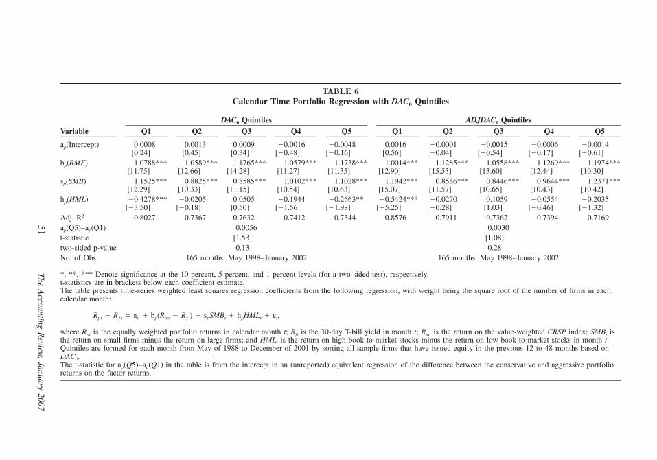
51T

heA

ccountingR

eview,

January2007

TABLE 6Calendar Time Portfolio Regression with DAC0 Quintiles

Variable

DAC0 Quintiles

Q1 Q2 Q3 Q4 Q5

ADJDAC0 Quintiles

Q1 Q2 Q3 Q4 Q5

ap(Intercept) 0.0008 0.0013 0.0009 �0.0016 �0.0048 0.0016 �0.0001 �0.0015 �0.0006 �0.0014[0.24] [0.45] [0.34] [�0.48] [�0.16] [0.56] [�0.04] [�0.54] [�0.17] [�0.61]

bp(RMF) 1.0788*** 1.0589*** 1.1765*** 1.0579*** 1.1738*** 1.0014*** 1.1285*** 1.0558*** 1.1269*** 1.1974***[11.75] [12.66] [14.28] [11.27] [11.35] [12.90] [15.53] [13.60] [12.44] [10.30]

sp(SMB) 1.1525*** 0.8825*** 0.8585*** 1.0102*** 1.1028*** 1.1942*** 0.8586*** 0.8446*** 0.9644*** 1.2371***[12.29] [10.33] [11.15] [10.54] [10.63] [15.07] [11.57] [10.65] [10.43] [10.42]

hp(HML) �0.4278*** �0.0205 0.0505 �0.1944 �0.2663** �0.5424*** �0.0270 0.1059 �0.0554 �0.2035[�3.50] [�0.18] [0.50] [�1.56] [�1.98] [�5.25] [�0.28] [1.03] [�0.46] [�1.32]

Adj. R2 0.8027 0.7367 0.7632 0.7412 0.7344 0.8576 0.7911 0.7362 0.7394 0.7169ap(Q5)–ap(Q1) 0.0056 0.0030t-statistic [1.53] [1.08]two-sided p-value 0.13 0.28No. of Obs. 165 months: May 1998–January 2002 165 months: May 1998–January 2002

*, **, *** Denote significance at the 10 percent, 5 percent, and 1 percent levels (for a two-sided test), respectively.t-statistics are in brackets below each coefficient estimate.The table presents time-series weighted least squares regression coefficients from the following regression, with weight being the square root of the number of firms in eachcalendar month:

Rpt � Rƒt � ap � bp(Rmt � Rƒt) � spSMBt � hpHMLt � εt,

where Rpt is the equally weighted portfolio returns in calendar month t; Rft is the 30-day T-bill yield in month t; Rmt is the return on the value-weighted CRSP index; SMBt isthe return on small firms minus the return on large firms; and HMLt is the return on high book-to-market stocks minus the return on low book-to-market stocks in month t.Quintiles are formed for each month from May of 1988 to December of 2001 by sorting all sample firms that have issued equity in the previous 12 to 48 months based onDAC0.The t-statistic for ap(Q5)–ap(Q1) in the table is from the intercept in an (unreported) equivalent regression of the difference between the conservative and aggressive portfolioreturns on the factor returns.

52 Fan


The estimated difference in intercepts between the conservative and aggressive portfoliosand associated t-statistics is obtained from an unreported time-series regression of the dif-ference in returns between the conservative and aggressive portfolios on the factor returns.The calculated abnormal returns differential between the most aggressive and most con-servative discretionary accruals portfolios is 0.56 percent per month, implying an annualreturn differential of 6.72 percent (0.56 percent * 12).

Table 6 also shows the calendar-time portfolio regression results when the issue-yearperformance-adjusted discretionary accruals (ADJDAC0) is used to determine the portfolioformation. No monotonically declining pattern from Q1 to Q5 is discernable. The statisticaland economic significance of the abnormal return differential between the conservative (Q1)and aggressive portfolio (Q5) is further reduced. The two-tailed p-value for the differencein intercepts between the aggressive and conservative earnings management portfolios is0.40, and the annual abnormal returns differential is 3.6 percent (0.30 percent * 12).

To summarize, even though Section VI shows that there is strong evidence that theissue-year discretionary accruals predict the post-issue deterioration in IPO firms’ operatingperformance measures, there is no strong evidence that discretionary accruals estimatedfrom cash flow statement and post-issue abnormal stock returns are negatively correlated.Performance matching further weakens the statistical and economic significance of therelationship between the two. This lack of intertemporal and methodological robustnessdiminishes our confidence in TWW and TWR’s conclusion that the market is misled byincome-increasing accrual management in the IPO year.

VII. TESTS OF IPO PRICING: H2Hypothesis 2 predicts that both reported earnings and ownership retention should be

positively priced by investors in valuing IPO firms. To test this hypothesis, I employ anempirical formulation that is motivated by the model and intuition of Ohlson (1995) andDownes and Heinkel (1982). I posit that the initial market value of equity is a function ofnet income, the book value of equity, the ownership retention signal, and the total grossproceeds raised during the IPO process.

To set the stage, I first run OLS regressions according to the following empiricalformulation:

V � w � w � � w Gross Proceeds � w Net Income �w Book Value , (13)i 0 1 i 2 i 3 i 4 i

where:

Vi � market value of IPO firm i immediately after the offering, calculated astotal number of shares outstanding after the offer multiplied by closingprice on the first day of trading;

�i � ownership retention measure as defined in Section V;Net Incomei � IPO firm i’s net income before extraordinary items (#123 from Cash

Flow Statement) in year �1;Book Valuei � IPO firm i’s book value of equity (#60) in year �1; and

Gross Proceedsi � offer price multiplied by total number of primary shares issued.

Only firms with positive pre-offering book values are included in the regression. Tomitigate the effect of heteroscedasticity and scale bias, I also use weighted least squares



TABLE 7Tests of IPO Pricing

Variables

Market Value: Vi

Ordinary Least SquaresCoefficient Coefficient

Weighted Least SquaresCoefficient Coefficient

Intercept �151.250*** �312.230*** �423.479*** �648.557***[�6.20] [�15.69] [�13.00] [�98.92]

� 380.740*** 469.090*** 905.891*** 1710.071***[10.71] [16.52] [20.07] [28.46]

Net Income 1.850*** 1.354*** 1.960*** 1.480***[9.32] [4.28] [7.24] [7.41]

Book Value 2.280*** 0.732*** 2.168*** 0.567***[27.47] [9.59] [29.44] [8.09]

Gross Proceeds 4.402*** 4.442***[37.24] [39.38]

Adj. R2 0.3390 0.6995 0.4920 0.7451Prob(F) �0.0001 �0.0001 �0.0001 �0.0001No. of Obs. 1295 1288 1276 1266

*, **, *** Denote significance at the 10 percent, 5 percent, and 1 percent levels (for a two-sided test),respectively.t-statistics are in brackets below each coefficient estimate. To reduce the influence of outliers, all variables in theregressions are trimmed at top and bottom 1 percent. I also eliminate from each regression all influentialobservations meeting one of the following conditions: absolute value of DFFITS greater than 2, absolute valueof STUDENT greater than 2, or COOKD greater than 2 (Belsley et al. 1980).Variable Definitions:The dependent variable is Vi, which is market value of the IPO firm i immediately after the offering, calculatedas total number of shares outstanding after the offer * closing price on the first day of trading.The independent variables are:

�i � ownership retention measure as defined in Section V;Net Incomei � IPO firm’s net income before extraordinary items (#123, from Cash Flow Statement) in year

�1;Book Valuei � IPO firm’s book value of equity (#60) in year �1; and

Gross Proceedsi � offer price * total number of primary shares issued.Columns 2–3 are results from Ordinary Least Squares. All observations used in the regression have positivebook values.Columns 4–5 are results from Weighted Least Squares, with weight being lagged sales. All observations used inthe regression have positive book values and non-missing lagged sales.

with weight being the total revenue in year �1 to re-estimate the above empirical formu-lation. Table 7 shows that the coefficients on Net Income and Ownership Retention (�) aresignificantly positive in all regression specifications.

In summary, consistent with H2, for the sample of IPO firms examined here, there isstrong evidence that both ownership retention and Net Income are significantly positivelyrelated to IPO valuation.

VIII. TESTS OF THE TRADE-OFF BETWEEN EARNINGS MANAGEMENTAND OWNERSHIP RETENTION: H3

I test H3 by the following system of equations with discretionary accruals and retainedownership as dependent variables, each modeled as a function of the other signal, the exante risk measure (STDRET), and a set of control variables. More specifically, for theregression of ownership retention:

54 Fan


lgALPHA � �0 � �1STDRET � �2DAC0 � �3UnderP � �4LEV � �5CAPEXP01

� �6UWrank � �7lgAge � �8VCdum � �9Hitech � �iYr(i)96�

i�87

� ε1,

and for the regression of earnings management regression:

DAC0 � �0 � �1STDRET � �2lgALPHA � �3ACCSALES � �4LEV � �5CAPEXP01

� �6UWrank ��7lgAge � �8Auditor � �9VCdum � �10Hitech

� �iYr(i) � ε2,96�

t�87

where:27

lgALPHA � logit transformation of ownership retention � (defined in Section V), i.e.,lgALPHA � log(� / (1 � �));28

DAC0 � discretionary accruals estimated from the Modified Jones model;STDRET � average standard deviation of daily stock returns of the industry- and size-

matched control sample over the year prior to the IPO, as defined in SectionV;

UnderP � IPO underpricing, defined as the percentage difference between the offerprice and the closing price on the first day of trading;

LEV � IPO firm’s leverage ratio at the beginning of the IPO year, which equals 1minus the ratio of book value of equity (#60) to total assets (#6);

ACCSALES � issue-year total accruals per dollar of sales, where total accruals is measuredas ACC � EBXI (#123) � CFO (#308 � #124), as in Section V;

CAPEXP01 � average capital expenditure (#128) in year 0 and year 1, scaled by totalassets at the beginning of the issue-year (year 0);

lgAge � log(1 � IPO Age), where IPO firm age is calculated as the difference be-tween the founding year and IPO issue-year;

UWrank � a ranking of the reputation of the lead underwriter on a 0–9 scale followingCarter et al. (1998), 9 being the highest;29

Auditor � indicator variable for auditor reputation, which equals 1 if the auditor is oneof the Big 5 (Big 6) auditors;

VCdum � indicator variable that equals 1 if the IPO firm is backed by venture capital(VC); and

Hitech � indicator variable from SDC that equals 1 if the IPO firm is in the high-techindustry, and 0 otherwise.

The key variable of interest in this context is STDRET. According to H3, as the riskof the IPO firm increases, it becomes relatively costlier for the risk-averse issuer to retain

27 Compustat data item are included in parentheses.28 Because the ratio variable � is bounded by 0 and 1 and is highly skewed, logit transformation is used to normalize

the distribution.29 The ranking is obtained from Jay Ritter’s website, which is constructed for the 1992–2000 period. When an

IPO issuer has multiple lead underwriters, the average ranking is used instead.



shares of the IPO firm, and the issuer will substitute earnings management for ownershipretention so as to communicate his private information at minimal cost. To test this cross-sectionally, however, one would have to control for other effects that are not explicitlymodeled in the restricted theoretical setting.

Starting with the ownership retention regression, underpricing (UnderP) is included asa control variable in the ownership retention regression as prior literature suggests that itis an important determinant of post-IPO ownership structure. For example, Brennan andFranks (1997) argue that issuers underprice their firms at the IPO to induce oversubscrip-tion, which allows the firm to discriminate against large blockholders in the allocation ofshares. In their theoretical model of IPOs, Grinblatt and Hwang (1989) show that, holdingthe riskiness of the firm constant, ownership retention and underpricing are positively cor-related. Beatty (1989) also empirically confirms a positive and significant relationship be-tween retained ownership and underpricing. According to the pecking-order theory of cap-ital structure (Myers and Majluf 1984), firms prefer internal finance to external finance anddebt finance to equity finance. Hence, a high-growth firm may be forced to finance itsinvestment decisions by equity instead of retained earnings or debt. I use the IPO firm’sasset-scaled average capital expenditure in year 0 and year 1 (CAPEXP01) as a growthproxy and therefore I predict that CAPEXP01 should be negatively related with ownershipretention. Relatedly, limited debt capacity may motivate the firm to raise more equitythrough the IPO process. Hence, I predict that IPO firms with higher pre-IPO leverageratios will have lower post-IPO ownership retention. Underwriter rank (UWrank) is includedto control for the investment bank’s reputation in facilitating shareholders’ selling. As VCsmight take IPOs as an exit opportunity to realize their stake in the firm, I predict that VCbacking is associated with less ownership retention. I also include lgAge, a high-tech in-dustry dummy (Hitech) and a set of IPO-year dummies to control for systematic differencesin firm characteristics and time-period differences.

A somewhat similar set of control variables is included in the earnings managementregression. These control variables can be classified into two categories: (1) third-partycertification and monitoring, and (2) incentive and opportunities for earnings manipulation.The first category includes auditor and investment banker reputation and a dummy variableindicating the presence of venture capital backing. All other things equal, an auditorand/or investment banker with a lower reputation may be more acquiescent to the issuer’smanagement of earnings. Hochberg (2004) provides evidence that venture capital backingis associated with a reduction in earnings management in the IPO year, suggesting thatventure capitalists might play a positive role in governing and monitoring the firm due totheir unique expertise and knowledge. I thus predict that the coefficients on the auditorreputation (Auditor), the investment banker reputation (UWrank) and the VC backingdummy (VCdum) are negative. The second category of variables include leverage ratio(LEV), total accruals per dollar of sales (ACCSALES), average capital expenditure in year0 and year 1 scaled by total assets at the beginning of year 0 (CAPEXP01), and lgAge.Leverage ratio (LEV) is included to control for the documented tendency of firms to manageearnings upward in order to loosen debt covenant constraints (DeFond and Jiambalvo 1994).The total accruals per dollar of sales in the issue-year (ACCSALES) is used as a proxy forthe accounting flexibility the IPO issuer has in manipulating earnings. I expect that moreaccounting flexibility is associated with a higher degree of earnings management. lgAgeand CAPEXP01 are used as proxies for growth. Younger and high-growth firms derive asubstantial part of their value from highly uncertain growth opportunities, making it harderfor investors to appraise such firms and easier for managers of these firms to mislead

56 Fan


investors.30 I thus expect capital expenditure growth to be positively associated with earn-ings management and firm age to be negatively associated with earnings management.

To summarize, besides STDRET, the control variables that are common to both regres-sions are: UWrank, VCdum, CAPEXP01, LEV, lgAge, and a set of IPO-year dummies. Un-derpricing (UnderP) appears only in the ownership retention regression, and ACCSALESand auditor reputation (Auditor) appear only in the earnings management regression.

It is important to address the simultaneity issue between the two equations since in mymodel, ownership retention and earnings management are jointly determined in that thestrategic mix of the two is chosen to minimize the total signaling cost. Failing to controlfor such simultaneity in the design of empirical tests leads to biased estimates in both theexogenous, as well as endogenous, variables (Intriligator et al. 1996). Thus, I estimatethese two equations by two-stage least squares (2SLS). In this case, UnderP is the exo-genous variable directly related to ownership retention, and Auditor and ACCSALES areexogenous variables that are directly related to earnings management. Hence, the two-equation system is fully identified.

Columns 1 and 3 in Table 8 present the first-stage regression of ownership retentionand earnings management on all exogenous variables. The adjusted R2s are 13.35 percentand 38.82 percent, respectively, both with prob(F) � .0001, indicating that the instrumentsare jointly significant.

The second-stage regression results are presented in columns 2 and 4. The coefficientson STDRET remain significantly negative in the ownership retention regression (two-tailedp-value � 0.02), and significantly positive in the earnings management regression (two-tailed p-value).

Table 9 presents the two-stage least squares regression results using the issue-yearperformance-adjusted discretionary accruals (ADJADC0). As predicted, the coefficient onSTDRET is significantly negative in the ownership retention regression (two-tailed p-value� 0.05), and is significantly positive in the earnings management regression (two-tailed p-value � 0.01). Performance matching, however, reduces the R2 of the second-stage earningsmanagement regression from 38.82 percent to 20.01 percent. The reduction in explanatorypower should probably be expected, given that performance matching reduces measurementerror in discretionary accruals that correlates with the growth proxies used in the regression,resulting in much less variation in the dependent variable ADJADC0 being explained. Inthe earnings management regression, the variables intended to capture the incentives andconstraints of aggressive accounting, ACCSALES, LEV, CAPEXP01, and lgAge, all have theexpected signs, but only ACCSALES and LEV are statistically significant. The third-partymonitoring and certification variables, UWrank and VCdum have the expected signs but arestatistically insignificant at conventional levels. Inconsistent with the prediction, the coef-ficient on the auditor dummy (Auditor) is positive, but is statistically insignificant. In theownership retention regression, all variables have expected signs except UWrank, which issignificantly positive.

In summary, I interpret the above results as generally consistent with the hypothesisthat riskier firms will resort more to earnings management and retain less ownership toachieve separation in the signaling equilibrium.

30 Beneish (1999) also reports that fast-growing firms have strong incentives to manipulate financial statements toallay the perception of growth deceleration.



TABLE 8Two-Stage Least Squares Regression with DAC0

VariablelgALPHA

First Stage Second StageDAC0

First Stage Second Stage

Intercept 0.888*** ? �0 0.890*** 0.062 ? �0 0.071*[7.07] [7.07] [1.53] [1.64]

STDRET �4.340*** � �1 �4.493** 1.295** � �1 1.410**[�2.62] [�2.53] [2.42] [2.51]

DAC0 ? �2 �0.251**[�2.24]

lgALPHA ? �2 �0.013[�1.24]

UNDERP 0.381*** � �3 0.179** �0.025[4.21] [2.31] [�0.85]

ACCSALES �0.086* 0.348*** � �3 0.508***[�1.67] [22.82] [22.98]

LEV �0.039* � �4 �0.049** 0.016 � �4 0.021***[�1.78] [�2.45] [0.36] [2.66]

CAPEXP01 �0.001 � �5 �0.590*** 0.001*** � �5 0.003[�0.94] [�7.34] [0.28] [0.66]

UW Rank 0.022*** � �6 0.036*** �0.008*** � �6 �0.006***[2.98] [2.13] [�3.46] [�2.58]

lgAge �0.046*** ? �7 �0.047** �0.001 � �7 �0.007[�2.58] [�2.46] [�0.16] [�1.07]

Dummy: Auditor �0.044 0.003 � �8 �0.003[�0.70] [0.15] [�0.13]

Dummy: VC backed �0.064** � �8 �0.055** �0.011 � �9 �0.012[�1.85] [�2.17] [�1.05] [�0.99]

Dummy: Hitech 0.180*** ? �9 0.127*** 0.005 ? �10 0.000[5.11] [4.02] [0.47] [0.03]

Year Dummies Included Included Included Included

Adjusted R2 0.1335 0.1574 0.3282 0.3882Prob(F) �0.0001 �0.0001 �0.0001 �0.0001No. of Observations 1098 942 1201 942

*, **, *** Denote significance at the 10 percent, 5 percent, and 1 percent levels (for a two-sided test),respectively.t-statistics are in brackets below each coefficient estimate.To reduce the influence of outliers, all variables in the regressions are trimmed at � /�1 percent. Influentialobservations meeting any of the following conditions are deleted: absolute value of DFFITS greater than 2,absolute value of STUDENT greater than 2, or COOKD greater than 2, per Belsley et al. (1980).All variables are defined in Section VIII.

VIII. SUMMARYThis paper examines, in a rational expectation framework, how ownership retention and

earnings management interact and how they jointly affect the valuation of IPO firms. An-alytically, it extends the univariate signaling framework of Leland and Pyle (1977) andderives an efficient signaling equilibrium in which both reported earnings and ownershipretention are endogenously chosen to convey an IPO issuer’s private information. It is shownthat even though either ownership retention or reported earnings communicates the issuer’s

58 Fan


TABLE 9Two-Stage Least Squares Regression with ADJDAC0

VariablelgALPHA

First Stage Second StageADJDAC0

First Stage Second Stage

Intercept 0.888*** ? �0 0.902*** �0.115 ? �0 �0.177**[7.07] [6.60] [�1.58] [�2.31]

STDRET �4.340*** � �1 �4.345** 3.093** � �1 3.712***[�2.62] [�2.20] [3.14] [3.65]

ADJDAC0 ? �2 �0.033[�0.56]

lgALPHA ? �2 �0.003[�0.19]

UNDERP 0.381*** � �3 0.478*** �0.201***[4.21] [4.35] [�3.69]

ACCSALES �0.086* 0.572*** � �3 0.618***[�1.67] [14.74] [13.64]

LEV �0.039* � �4 �0.057** 0.036** � �4 0.035**[�1.78] [�1.81] [2.34] [2.17]

CAPEXP01 �0.001 � �5 �0.317 0.010 � �5 0.008[�0.94] [�1.41] [0.88] [0.73]

UW Rank 0.022*** � �6 0.021*** 0.001 � �6 0.003[2.98] [2.57] [0.34] [0.66]

lgAge �0.046*** ? �7 �0.055** �0.007 � �7 �0.009[�2.58] [�2.79] [�0.69] [�0.87]

Dummy: Auditor �0.044 0.033 � �8 0.041[�0.70] [0.90] [1.15]

Dummy: VC backed �0.064** � �8 �0.080** �0.015 � �9 �0.020[�1.85] [�2.07] [�0.78] [�0.98]

Dummy: Hitech 0.180*** ? �9 0.150*** �0.016 ? �10 �0.029[5.11] [3.78] [�0.84] [�1.40]

Year Dummies Included Included Included Included

Adjusted R2 0.1335 0.1624 0.1936 0.2001Prob(F) �0.0001 �0.0001 �0.0001 �0.0001No. of Observations 1098 883 1201 883

*, **, *** Denote significance at the 10 percent, 5 percent, and 1 percent levels (for a two-sided test),respectively.t-statistics are in brackets below each coefficient estimate.To reduce the influence of outliers, all variables in the regressions are trimmed at � /�1 percent. Influentialobservations meeting any of the following conditions are deleted: absolute value of DFFITS greater than 2,absolute value of STUDENT greater than 2, or COOKD greater than 1, per Belsley et al. (1980).All variables are defined in Section VIII.

type to the market unambiguously, the issuer will strategically employ both signals toachieve separation at minimal cost. Comparative statics analysis also shows that the trade-off between earnings management and ownership retention depends critically on the un-certainty over future earnings. The theoretical analysis generates a rich set of empiricalimplications regarding earnings management, market efficiency, and IPO pricing. Throughsystematic econometric analysis, I confirm the major predictions of the model.



This paper seeks to make the following contributions to the literature: First, it proposesa non-opportunistic motive for earnings management around corporate events, and chal-lenges the traditional view that earnings management during the IPO period is synonymouswith managerial opportunism. Second, by examining how ownership retention and account-ing information are priced during the IPO process, it sheds some light on the valuation ofIPO firms. Third, by re-examining the evidence presented in TWW and TWR using adifferent IPO sample and a better measure of accruals, this study provides new evidenceregarding efficiency of the IPO market and suggests that care must be exercised in inter-preting results in prior studies.

APPENDIXProof of Proposition 1

Since the identities of each type of issuers are fully revealed in a separating equilibrium,�L has nothing to gain by bearing risk because there is no worse type to separate from.Hence we must have �L � 0. To determine the strategy of �H, we need to find the equityfraction that �H issuer must retain in order to deter �L issuer from mimicking him. In otherwords, we need to find the values of that satisfy the following incentive constraint:

bL H 2 2 L�� (1 � �)� � � � � .2

In the unique separating equilibrium that is Pareto-dominating, the optimal ownershipretention for �H is the smallest � that satisfies the above inequality, i.e.:

H L H L 2 H L�(� � � )(� � � � 2b� ) � � � �H� � 2b�

Proof of Proposition 2

1) obvious.2) When � � �*, truthful reporting constitutes an equilibrium.

To show this, I check whether given the market’s beliefs, �L has no incentive to pretendthat he is �H. The benefit for �L to report eH is that for the (1 � �) share of the firm sold,he would be valued as �H instead of �L, and get an increase in cash receipts of (1 � �)(�H

� �L). The cost for �L to report eH is that for the � share of the firm he retains, the valueof the firm decreases by the cost of such manipulation, �C(eH � eL). Hence, �L would notwant to pretend to be �H by reporting rH � eH if �C(eH � eL) � (1 � �)(�H � �L), orequivalently, � � �*. In other words, there is a ‘‘costless,’’ perfectly informative equilibriumwhen � � �*.

3) When � � �*, there exists a fully separating equilibrium in which �H reports rH(�)� eH, and the low-type truthfully reports rL � eL.

Define rH(�) as such so that �C(rH(�) � eL) � (1 � �)[�H � C(rH(�) � wH)� �L].

To show that there indeed exists such an equilibrium, I again check whether the low-type has an incentive to mimic the high-type by reporting rH. The cost of mimicking thehigh-type’s earnings report is �C(rH(�) � eL) since for the � share of the firm retained, the

60 Fan


firm value decreases by C(rH � eL). The benefit of mimicking the high-type’s earningsreport is (1 � �)[�H � C(rH(�) � eH) � �L] since for the (1 � �) shares of the firm sold,the IPO firm is valued as �H � C(rH � eH) instead of �L. Thus, by over-reporting to rH

� rH(�) so that �C(rH � eH) � (1 � �)[�H � C(rH � eH) � �L], �H deters �L frommimicking his earnings report. Notice that given � � �*, to make the equality hold, rH

must be greater than eH and the market’s rational valuation of the high-type firm, �H

� C(rH � eH), must be greater than �L. Further, such rH is decreasing in � as after re-

arranging the terms, the equality becomes C(rH � eH) � C(rH � eL) � �H � �L.�

1 � �Then as � decreases, rH must increase to make the equality hold.

4) There is no pooling equilibrium that satisfies Cho-Kreps Intuitive Criterion.A Pooling (Perfect Bayesian) Equilibrium is defined as follows:● Issuer’s strategy: rH � rL � eH

● Market’s belief: Upon observing r � eH, the market believes that the issuer is�L with probability and is �H with probability (1 � ). Then the IPO pricewould be Pp(eH) � [�L � C(eH; �L)] � (1 � )�H and I am free to specify theoff-equilibrium-path beliefs such that this indeed constitutes an equilibrium.

To check whether the pooling equilibrium survives the Cho-Kreps Intuitive Criterion,I need to show the following:

First, I show that there exists a rs � eH such that the following is true:

H s H L s L(1 � �)[� � C(r � e )] � �[� � C(r � e )]p H L H L� (1 � �)P (e ) � �[� � C(e � e )] (A-1)

Notice that the left-hand side is the payoff to �L if he deviates from the equilibriumpath by reporting rs � eH and the market believes that he is �H. The right-hand side is thepayoff to �L by staying on the equilibrium path, i.e., reporting eH and being pooled with�H. When rs � eH, the left-hand side becomes (1 � �)�H � �[�L � C(eH � eL)]. Itimmediately follows that the left-hand side is greater than the right-hand side since �H

� Pp(eH). Increasing rs above eH would decrease the left-hand side. Given that C is in-creasing in r, there exists a rs � eH such that (A-1) holds.

Second, I show that for such rs that satisfies (A-2), the following holds:

H s H p H H� � C(r � e ) � (1 � �)P (e ) � �� . (A-2)

Notice that the left-hand side of (A-2) is the payoff to �H if he deviates to report rs

and the market believes that he is �H. The right-hand side of (A-2) is the payoff to �H ifhe stays on the equilibrium path and is pooled with �L.

Subtracting (A-1) from both sides of (A-2) and rearranging terms, I have C(rs � eL)� C(rs � eH) � C(eH � eL). Since C � � 0, the above equality holds for any rs � eH, sothe rs that satisfies (A-1) also satisfies (A-2). Thus, the pooling equilibrium does not survivethe Cho-Kreps Intuitive Criterion because �H could make the following statement:

I am �H. To prove this, I am reporting my current earnings as rs � eH. Notice that if Iam �L, I would never want to do this because even if you believe that I am �H, I wouldbe strictly worse off than staying on the equilibrium path (reporting eH and pooled with�H). But if you believe that I am indeed �H, then I would be better off than staying onthe pooling equilibrium path, so you should believe that I am �H.



Proof of Proposition 3Let � denote the non-negative multiplier of the non-mimicry constraint in (6) and �

denote the non-negative multiplier of the � � 0 constraint.Notice that the first-order conditions of �H’s constrained optimization problem can be

written as:

H L HC � �[�C � (1 � �)C ] � 0; (A-3)r r r

2 L L H H 2�b�� [� � C (r) � � � C (r) � b�� ] � � � 0. (A-4)

If, for �H, the optimum under perfect information, � � 0 and r � eH had satisfied thenon-mimicry constraint, then � � 0, r � eH would have been the signaling choices of firmH, and the resulting efficient signaling equilibrium would have entailed no welfare loss dueto signaling; it would have been a costless signaling equilibrium. However, (0, eH) violatesthe non-mimicry constraint as �H � �L. Further, as � � 0 yields the earnings report unin-formative because the issuer does not bear any of the costs associated with over-reportingearnings, in the optimal solution, � must be greater than 0. By the Kuhn-Tucker conditionand by complementary slackness, �� 0, so we must have � � 0 in the optimizationproblem.

Next, since � � 0, �L � CL(r) � �H � CH(r) � b��2 � 0. It follows that � � 0 in

order to satisfy (A-4). From (A-3), � � Notice that if r � eH, thenHCr H. CrL H�C � (1 � �)Cr r

� 0 and � � 0, so it must be that � 0, i.e., r � eH. In summary, even though either �HCr

or r could communicate the issuer’s type to the market unambiguously (as discussed inSection III), in the efficient signaling equilibrium, the higher value issuer will strategicallyemploy both signals to achieve separation at minimal cost.

Proof of Proposition 4Combining (A-3) and (A-4), I obtain:

H 2C b��r� � � . (A-5)L H L L H H 2�C � (1 � �)C �� C (r) � � � C (r) � b��r r

As � � 0, the non-mimicry constraint is binding, so we must also have:

bL L H H 2 2 L�[� � C (r)] � (1 � �)[� � C (r)] � � � � � . (A-6)2

After rearranging, I obtain the following two equations:

H H L L H 2 2 L HC [� � � � C (r) � C (r)] � b� � (C � C ) � 0; (A-7)r r r

bL L H H 2 2 L�[� � C (r)] � (1 � �)[� � C (r)] � � � � � � 0. (A-8)2

Notice that (A-7) is derived from the necessary conditions for the minimization of totalsignaling costs—the marginal rate of substitution of each signal must be equalized, whereas(A-8) is the ‘‘non-mimicry’’ condition.

62 Fan


Let:

1 H H L L H 2 2 L HF � C [� � � � C (r) � C (r)] � b� � (C � C ); (A-9)r r r

b2 L L H H 2 2 LF � �[� � C (r)] � (1 � �)[� � C (r)] � � � � � . (A-10)2

Then must satisfy the system of equations:�� r

,2 2��

�� r1 1 1F � F � F � 0; (A-11)2� r �2 2��

�� r2 2 2F � F � F � 0. (A-12)2� r �2 2��

Differentiating the above F1 and F2 with respect to �, r, and �2, I obtain:

1 L H 2F � �2(C � C )b� � � 0; (A-13)� r r

1 H L L H H H L H L H 2 2 31F � (� � � � C � C )C � C (C � C ) � (C � C )b� � � 0;r rr r r r rr rr

(A-14)

1 L H 2F � �(C � C )b� � 0; (A-15)2� r r

2 L L H H 2F � (� � C (r) � � � C (r)) � b�� 0; (A-16)�

2 L HF � �(�C � (1 � �)C ) � 0; (A-17)r r r

b2 2F � � � � 0. (A-18)2� 2

By Cramer’s rule, I have:

1 2 2 1F F � F F2 2r � r �2��(� ) � ; (A-19)1 2 1 2F F � F F� r r �

2 1 1 2F F � F F2 2� � � �2r�(� ) � . (A-20)1 2 1 2F F � F F� r r �

It is obvious that � � 0 and, � � 0 given the signs of the1 2 2 1 1 2 1 2F F F F F F F F2 2r � r � � r r �

individual components. After simplification, � equals b�2 � [�L2 1 1 2 H LF F F F (C C )2 2� � � � r r

31 By the convexity of C, it immediately follows that (�H � �L � CL � CH ) � ( � � 0. When C�H H L HC C C C )rr r r r

� 0, Thus, � 0.L H 1C C . Frr rr r



� CL(r) � �H � CH(r)], which is greater than 0 since � and �L � �H. Thus, ��(�2)H LC Cr r

� 0 and r�(�2) � 0.

REFERENCESBarber, B. M., and J. D. Lyon. 1996. Detecting abnormal operating performance: The empirical power

and specification of test statistics. Journal of Financial Economics 41 (July): 359–399.———, and ———. 1997. Detecting long-run abnormal stock returns: The empirical power and

specification of test statistics. Journal of Financial Economics 43 (March): 341–372.Beatty, R. 1989. Auditor reputation and the pricing of initial public offerings. The Accounting Review

64 (October): 693–709.Belsley, D., E. Kuh, and R. Welsch. 1980. Regression Diagnostics. New York, NY: John Wiley &

Sons Inc.Beneish, M. D. 1999. The detection of earnings manipulation. Working paper, Indiana University.Brennan, M., and J. Franks. 1997. Underpricing, ownership and control in initial public offerings of

equity securities in the UK. Journal of Financial Economics 45 (September): 391–413.Carter, R. B., F. H. Dark, and A. K. Singh. 1998. Underwriter reputation, initial returns, and the long-

run performance of IPO stocks. Journal of Finance 53 (February): 285–311.Cho, I. K., and D. M. Kreps. 1987. Signaling games and stable equilibria. The Quarterly Journal of

Economics 102 (May): 179–222.Collins, D. W., and P. Hribar. 2002. Errors in estimating accruals: Implications for empirical research.

Journal of Accounting Research 40 (March): 105–135.Copley, P. A., and E. B. Douthett. 2002. The association between auditor choice, ownership retained,

and earnings disclosure by firms making initial public offerings. Contemporary AccountingResearch 19 (Spring): 49–76.

Datar, S. M., G. A. Feltham, and J. S. Hughes. 1991. The role of audits and audit quality in valuingnew issues. Journal of Accounting and Economics 14 (March): 3–49.

Dechow, P. M., R. G. Sloan, and A. P. Sweeney. 1995. Detecting earnings management. The Ac-counting Review 70 (April): 193–225.

DeFond, M., and J. Jiambalvo. 1994. Debt covenant violation and manipulation of accruals. Journalof Accounting and Economics 17 (January): 145–176.

Downes, D. H., and R. Heinkel. 1982. Signaling and the valuation of unseasoned new issues. Journalof Finance 37 (March): 1–10.

Engers, M. 1987. Signalling with many signals. Econometrica 55 (May): 663–674.Fama, E. F., and K. R. French. 1993. Common risk factors in the returns on stocks and bonds. Journal

of Financial Economics 33 (February): 3–56.———. 1998. Market efficiency, long-term returns, and behavioral finance. Journal of Financial

Economics 49 (September): 283–306.Feltham, G. A., J. S. Hughes, and D. A. Simunic. 1991. Empirical assessment of the impact of auditor

quality on the valuation of new issues. Journal of Accounting and Economics 14 (December):375–399.

Field, L., and M. Lowry. 2004. How is institutional investment in initial public offerings related tothe long-run performance of these firms? Working paper, The Pennsylvania State University.

Franks, J., R. Harris, and S. Titman. 1991. Postmerger share-price performance of acquiring firms.Journal of Financial Economics 29 (March): 81–96.

Grinblatt, M., and C. Y. Hwang. 1989. Signalling and the pricing of new issues. Journal of Finance44 (June): 393–420.

Hochberg, Y. 2004. Venture capital and corporate governance in the newly public firm. Working paper,University of Rochester.

Hughes, P. J. 1986. Signalling by direct disclosure under asymmetric information. Journal of Ac-counting and Economics 8 (June): 119–142.

64 Fan


Intriligator, M., R. G. Bodkin, and C. Hsiao. 1996. Econometric Models, Techniques, and Applications.Upper Saddle River, NJ: Prentice Hall.

Jain, P. C., and O. Kini. 1994. The post-issue operating performance of IPO firms. Journal of Finance49 (December): 1699–1726.

John, K., and B. Mishra. 1990. Information content of insider trading around corporate announce-ments: The case of capital expenditures. Journal of Finance 45 (July): 835–855.

Kothari, S. P., and J. B. Warner. 1997. Measuring long-horizon security price performance. Journalof Financial Economics 43 (March): 301–339.

———, A. J. Leone, and C. E. Wasley. 2005. Performance matched discretionary accrual measures.Journal of Accounting and Economics 39 (February): 163–197.

Leland, H. E., and D. H. Pyle. 1977. Informational asymmetrics, financial structure, and financialintermediation. Journal of Finance 32 (May): 371–387.

Loughran, T., and J. Ritter. 1995. The new issues puzzle. Journal of Finance 50 (March): 23–52.Lowry, M., and S. Shu. 2002. Litigation risk and IPO underpricing. Journal of Financial Economics

65 (September): 309–335.McNichols, M., and G. P. Wilson. 1988. Evidence of earnings management from the provision for

bad debts. Journal of Accounting Research 26 (Supplement): 1–31.———. 2000. Research design issues in earnings management studies. Journal of Accounting and

Public Policy 19 (September): 313–345.Milgrom, P., and J. Roberts. 1986. Price and advertising signals of product quality. Journal of Political

Economy 94 (August): 796–821.Myers, S. C., and N. S. Majluf. 1984. Corporate financing and investment decisions when firms have

information investors do not have. Journal of Financial Economics 13 (June): 187–221.Ohlson, J. 1995. Earnings, book value and dividends in security valuation. Contemporary Accounting

Research 11: 661–687.Rangan, S. 1998. Earnings management and the performance of seasoned equity offerings. Journal

of Financial Economics 50 (October): 101–122.Riley, J. G. 1975. Competitive signalling. Journal of Economic Theory 10 (April): 174–186.Ritter, J. R. 1991. The long-run performance of initial public offerings. Journal of Finance 46 (March):

3–27.———, and I. Welch. 2002. A review of IPO activity, pricing, and allocations. Journal of Finance

57 (August): 1795–1828.Shivakumar, L. 2000. Do firms mislead investors by overstating earnings before seasoned equity

offerings? Journal of Accounting and Economics 29 (June): 339–371.Shumway, T. 1997. The delisting bias in CRSP data. Journal of Finance 52 (March): 327–340.———, and V. A. Warther. 1999. The delisting bias in CRSP’s NASDAQ data and its implications

for the size effect. Journal of Finance 54 (December): 2361–2379.Simunic, D., and M. Stein. 1987. Product Differentiation in Auditing: Auditor Choice in the Market

for Unseasoned New Issues. Research Monograph Number 13. Vancouver, Canada: The Ca-nadian Certified General Accountants Research Foundation.

Spence, M. 1973. Job market signaling. The Quarterly Journal of Economics 87 (August): 355–374.Stein, J. C. 1989. Efficient capital markets, inefficient firms: A model of myopic corporate behavior.

The Quarterly Journal of Economics 104 (November): 655–669.Teoh, S. H., I. Welch, and T. Wong. 1998. Earnings management and the long-run market performance

of initial public offerings. Journal of Finance 53 (December): 1935–1974.Teoh, S. H., T. J. Wong, and G. R. Rao. 1998. Are accruals during initial public offerings opportun-

istic? Review of Accounting Studies 3 (May): 175–208.Viswanathan, S. 1987. A multiple signalling model of corporate financial policy. Unpublished disser-

tation, Northwestern University.

Documents

THE ACCOUNTING REVIEW pp. 27–64 Earnings …haas.berkeley.edu/faculty/papers/fan_IPO.pdf · 27 THE ACCOUNTING REVIEW Vol. 82, No. 1 2007 pp. 27–64 Earnings Management and Ownership