Embed Size (px)
Citation preview

7/25/2019 Text: Investigating Statistical Concepts, Applications, and Methods
http://slidepdf.com/reader/full/text-investigating-statistical-concepts-applications-and-methods 1/428

7/25/2019 Text: Investigating Statistical Concepts, Applications, and Methods
http://slidepdf.com/reader/full/text-investigating-statistical-concepts-applications-and-methods 2/428
Chance/Rossman, 2015 ISCAM IIII
i
Acknowledgements
We would like to thank the following reviewers for their continued feedback and suggestions. They havegreatly improved the quality of these materials. We would like to especially thank Julie Clark of HollinsUniversity for her gracious and extensive attention to detail.
Doug Andrews, Wittenberg University; Julie Clark, Hollins University; David Cruz-Uribe,Trinity College; Jo Hardin, Pomona College; Allen Hibbard, Central College; Sharon Lane-Getaz, St. Olaf University; Tom Linton, Central College; Mark Mills, Central College; PaulRoback, St. Olaf College; Soma Roy, Cal Poly – San Luis Obispo; Michael Stob, Calvin College
Cover Design: Danna Currie, Grover Beach
Initial Solutions to Investigations: Chelsea Lofland, based on classroom notesInitial Exercise Compilation and Solutions: Julie ClarkCopy-editing Assistance: Virginia Burroughs
Companion Website: www.rossmanchance.com/iscam3/Online Resources include solutions to investigations, exercises, and additional investigations.Also see Resources for Instructors.
Copyright January 2016 Beth Chance and Allan RossmanSan Luis Obispo, California
ALL RIGHTS RESERVED. No part of this work covered by the copyright hereon may be produced or -used in any form or by any means – graphic, electronic, or mechanical, including photocopying,
recording, taping, Web distribution, information storage retrieval systems, or in any other manner – without the written permission of the authors.

7/25/2019 Text: Investigating Statistical Concepts, Applications, and Methods
http://slidepdf.com/reader/full/text-investigating-statistical-concepts-applications-and-methods 3/428
Chance/Rossman, 2015 ISCAM IIII Table of Contents
!
!"#$% '( )'*+%*+,
To The Student ................................................. ...................................................... ..................................... 3
Investigation A: Traffic Fatalities And Federal Speed Limits .................................................. .................. 4
Investigation B: Random Babies .............................................................................................................. 12 Chapter 1: Analyzing One Categorical Variable ...................................................................................... 19
Section 1: Analyzing A Process Probability .............................................. ................................... 20
Section 2: Normal Approximations For Sample Proportions ................................................ ....... 65
Section 3: Sampling From A Finite Population .................................................. .......................... 94
Chapter 2: Analyzing Quantitative Data .............................................. ................................................... 135
Section 1: Descriptive Statistics .................................................................................................. 136
Section 2: Inference For Population Mean ................................................................................. 150
Section 3: Inference For Other Statistics .................................................................................... 169 Chapter 3: Comparing Two Proportions .............................................. ................................................... 184
Section 1: Comparing Two Population Proportions ................................................................... 185
Section 2: Types Of Studies ...................................................... .................................................. 201
Section 3: Comparing Two Treatment Probabilities .................................................................. 210
Section 4: Other Statistics ................................................ ...................................................... ..... 226
Chapter 4: Comparisons With Quantitative Variables .................................................... ........................ 254
Section 1: Comparing Groups – Quantitative Reponse .............................................................. 255
Section 2: Comparing Two Population Means ........................................................................... 258
Section 3: Comparing Two Treatment Means .................................................... ........................ 271
Section 4: Matched Pairs Designs ..................................................... .......................................... 288
Chapter 5: Comparing Several Populations, Exploring Relationships ................................................... 319
Section 1: Two Categorical Variables ........................................................................................ 320
Section 2: Comparing Several Population Means ...................................................................... 337
Section 3: Relationships Between Quantitative Variables ..................................................... ..... 354
Section 4: Inference For Regression ........................................................................................... 382
Index ..................................................... ...................................................... .......................................... 426
7/25/2019 Text: Investigating Statistical Concepts, Applications, and Methods
http://slidepdf.com/reader/full/text-investigating-statistical-concepts-applications-and-methods 4/428
Chance/Rossman, 2015 ISCAM IIII To the Student
#
!- !./ 0!12/3!
$%&%'(%')( '( & *&%+,*&%')&- ()',.),/
0-%+123+ %+'( '( & 4,56 (+15% (,.%,.),7 8,5+&8( & (,-9:,4';,.% 1.,7 &.; ),5%&'.-6 1., 19 %+, (+15%,(% %+&%
612 <'-- 9'.; '. %+'( =11>7 <, <&.% %1 ;5&< 6125 &%%,.%'1. %1 (,4,5&- %+'.3( &=12% '%? We use the singular “is” and not the plural “are.” It is certainly grammatically correct and mo 5,common usage to say “statistics are...”, but that use of the term refers to statistics as numerical values.@. %+'( (,.%,.), <, *,&. (%&%'(%')( &( & 9',-; 19 (%2;67 1., %+&% +&( '%( 1<. )1.),8%( &.; %,)+.'A2,(7&.; 1., %+&% )&. =, ,B)'%'.3 %1 (%2;6 &.; 85&)%'),/
We use “mathematical” as an adjective. Statistics certainly makes use of much mathematics, but it is a(,8&5&%, ;'()'8-'., &.; .1% & =5&.)+ 19 *&%+,*&%')(/ C&.67 8,5+&8( *1(%7 19 %+, )1.),8%( &.;*,%+1;( '. (%&%'(%')( &5, *&%+,*&%')&- '. .&%25,7 =2% %+,5, &5, &-(1 *&.6 %+&% ;1 .1% '.41-4,*&%+,*&%')(/ D12 <'-- (,, &. ,B&*8-, 19 %+'( ,&5-6 '. %+, =11> &( 612 (%2;6 %+, ;'99,5,.), =,%<,,.1=(,54&%'1.&- (%2;',( &.; )1.%51--,; ,B8,5'*,.%(/ D12 <'-- 9'.; %+&% ,4,. '. )&(,( <+,5, %+,*&%+,*&%')&- &(pects of two situations may be identical, the scope of one’s conclusions depends
)52)'&--6 1. +1< %+, ;&%& <,5, )1--,)%,;7 & (%&%'(%')&- 5&%+,5 %+&. & *&%+,*&%')&- )1.(';,5&%'1./ We use the noun “science.” Statistics is the science of gaining insight from ;&%&/ E&%& &5, F.1%'), %+,
8-25&- +,5,G 8',),( 19 '.915*&%'1. F19%,. =2% .1% &-<&6( .2*,5')&-G 3&%+,5,; 1. 8,18-, 15 1=H,)%( 15851),((,(/ I+, ()',.), 19 (%&%'(%')( '.41-4,( &-- &(8,)%( 19 '.A2'56 &=12% ;&%&/ J,--:;,('3.,; (%2;',(=,3'. <'%+ & 5,(,&5)+ A2,(%'1. 15 +681%+,('(7 ;,4'(, & 8-&. 915 )1--,)%'.3 ;&%& %1 &;;5,(( %+&% '((2,7851),,; %1 3&%+,5 %+, ;&%& &.; &.&-6K, %+,*7 &.; %+,. 19%,. *&>, '.9,5,.),( &=12% +1< %+, 9'.;'.3(3,.,5&-'K, =,61.; %+, 8&5%')2-&5 35128 =,'.3 (%2;',;/ $%&%'(%')( )1.),5.( '%(,-9 <'%+ &-- 8+&(,( 19 %+'(851),(( &.; %+,5,915, ,.)1*8&((,( %+, ()',.%'9') *,%+1;/
@. %+,(, *&%,5'&-(7 125 31&- '( %1 '.%51;2), 612 %1 %+'( 85&)%'), 19 (%&%'(%')(7 %1 +,-8 612 %+'.> &=12% %+,&88-')&%'1.( 19 (%&%'(%')( &.; %1 (%2;6 %+, *&%+,*&%')&- 2.;,58'..'.3( 19 %+, (%&%'(%')&- *,%+1;(/ C1(% 19
&--7 <, +18, 612 <'-- 9'.; 92. &.; ,.3&3'.3 ,B&*8-,(/ $%&%'(%')( '( & 4'%&--6 '*815%&.% (2=H,)%7 &.; &-(1 92.%1 (%2;6 &.; 85&)%'),7 -&53,-6 =,)&2(, '% =5'.3( 612 '.%1 )1.%&)% <'%+ &-- >'.;( 19 '.%,5,(%'.3 A2,(%'1.(/ D12<'-- &.&-6K, ;&%& 951* *,;')&- (%2;',(7 -,3&- )&(,(7 8(6)+1-136 ,B8,5'*,.%(7 (1)'1-13')&- (%2;',(7 &.; *&.6other contexts. To paraphrase the late statistician John Tukey, “the best thing about statistics is that it&--1<( 612 %1 8-&6 '. ,4eryone else’s backyard.” You never know what you might learn in a statistics class!
L., 19 %+, 9'5(% 9,&%25,( 612 <'-- .1%'), &=12% %+,(, *&%,5'&-( '( %+&% 612 <'-- 8-&6 %+, &)%'4, 51-, 19'.4,(%'3&%15/ D12 <'-- 5,&; &=12% &. &)%2&- (%2;6 &.; )1.(';,5 %+, 5,(,&5)+ A2,(%'1.7 &.; %+,. <, <'-- -,&;612 %1 ;'()14,5 &.; &88-6 %+, &885185'&%, %11-( 915 )&556'.3 12% %+, &.&-6('(/ 0 85'*&56 5,&(1. 915 %+,'.4,(%'3&%'4, .&%25, 19 %+,(, *&%,5'&-( '( %+&% <, (%51.3-6 =,-',4, %+&% 612 <'-- =,%%,5 2.;,5(%&.; &.; 5,%&'.%+, )1.),8%( '9 612 =2'-; 6125 1<. >.1<-,;3, &.; &5, ,.3&3,; '. %+, )1.%,B%/ M, (25, %1 &-(1 8&6 &%%,.%'1.%1 %+, $%2;6 N1.)-2('1.( %1 (,, +1< %1 ,99,)%'4,-6 )1.4,6 (%&%'(%')&- '.915*&%'1. &.; %+, O5&)%'), O51=-,*(915 %,(%'.3 6125 2.;,5(%&.;'.3/ I+123+ 612 <'-- 1.-6 ()5&%)+ %+, (259&), 19 %+, (%&%'(%')&- *,%+1;( 2(,; '.85&)%'),7 612 <'-- -,&5. 92.;&*,.%&- )1.),8%( F(2)+ &( 4&5'&='-'%67 5&.;1*.,((7 )1.9';,.),7 &.;('3.'9')&.),G %+&% &5, &. '.%,35&- 8&5% 19 *&.6 (%&%'(%')&- &.&-6(,(/ 0 ;'(%'.)% ,*8+&('( <'-- =, %+, 91)2( 1.+1< %+, ;&%& &5, )1--,)%,; &.; +1< %+'( ;,%,5*'.,( %+, ()18, 19 )1.)-2('1.( %+&% 612 )&. ;5&< 951* %+,;&%&/

7/25/2019 Text: Investigating Statistical Concepts, Applications, and Methods
http://slidepdf.com/reader/full/text-investigating-statistical-concepts-applications-and-methods 5/428
Chance/Rossman, 2015 ISCAM III Investigation A
Investigation A: Traffic Fatalities and Federal Speed Limits
I+,(, 9'5(% %<1 '.4,(%'3&%'1.( 3'4, 612 & 4,56 =5',9 '.%51;2)%'1. %1 (1*, ='3 ';,&( 915 %+, )125(,/ $1*, 19 612<'-- +&4, (,,. (1*, 19 %+,(, ';,&( =,915, &.; )&. 2(, %+, '.4,(%'3&%'1.( %1 5,95,(+ 6125 *,*156/ $1*, 19 %+,';,&( *&6 =, .,< &.; 612 <'-- (,, %+,* &3&'. '. -&%,5 )+&8%,5(/ Q15 .1<7 %56 %1 91)2( 1. %+, ='33,5 8')%25, 19&.&-6K'.3 ;&%& &.; ;5&<'.3 &885185'&%, )1.)-2('1.(/
Increases and decreases in motor vehicle fatalities can be monitored to help assess impacts of changes in policy. For example, in 1974, the US Federal government passed the National Maximum Speed Law,capping the speed limit on all interstate roads to 55mph. At the time, the goal was to improve fuelconsumption in response to the 1973 oil embargo. However, when Congress repealed this law in 1995,allowing states to raise the legal speed limit, many wondered if that would also lead to an increase inaccidents and fatalities. Frieman, Hedeker, and Richter (2009) took data from the Fatality AnalysisReporting System (FARS) to explore this issue, focusing in particular on the repeal of federal speedlimit controls on road fatalities.
(a) To the right is a portion of Wikipedia ’s “List of motor vehicle deaths inthe U.S. by year ” data (through 2013) on the number of total motor vehicledeaths in the United States per year. Notice the data are given in a datatable : each row represents a different year and the second column is thenumber of deaths in the U.S. that year. Suggest a research question thatyou could investigate with the full dataset.
(b) From the data provided here, do you see any trend or pattern to how thenumber of deaths per year is changing? Does this pattern make sense?What other information would you like to consider?
A time plot is a natural way to examine how a variable changes over time, but not about how other variables are also changing over the same time period. In particular, there are a lot more drivers on the roads now than in1899, which is going to impact the number of deaths, so we really shouldtake that into account. Typically, data like this would be scaled in someway, such as dividing by number of vehicle miles traveled by all cars thatyear or by the population size of the United States that year.

7/25/2019 Text: Investigating Statistical Concepts, Applications, and Methods
http://slidepdf.com/reader/full/text-investigating-statistical-concepts-applications-and-methods 6/428
Chance/Rossman, 2015 ISCAM III Investigation A
R
Below is a time plot of fatalities per 100,000 population using Wikipedia’s data from 1899 to 2013.
(c) Write a few sentences summarizing how this new variable was calculated and what you learn fromthe time plot of these data.
(d) In 1973 (before the speed limit was capped at 55 mph nationwide), the data report 25.507 fatalities per 100,000 people, compared to 21.134 in 1974 (after the national limit). Did the rate of fatalitiesdecrease between these two years? If so, by how much? Does that appear to be a “large” difference?How are you deciding?
Absolute differences , like you calculated in (d), can be difficult to evaluate , especially if you don’t
consider the magnitude of values they come from. You might respond differently to a box of M&Mscoming up 4 candies short, than to a difference of 4 fatalities per 100,000 people (about 10,000 moredeaths across the U.S. in one year). One way to take into account the magnitude of the data values youare comparing is to compute the percentage change :
percentage change = (current rate – previous rate) ! 100% previous rate
(e) Calculate and interpret this value. In particular, is this a positive or negative value; what does thatimply?

7/25/2019 Text: Investigating Statistical Concepts, Applications, and Methods
http://slidepdf.com/reader/full/text-investigating-statistical-concepts-applications-and-methods 7/428
Chance/Rossman, 2015 ISCAM III Investigation A
Below is a time plot of the year-to-year percentage change, starting in 1900.
(f) Why doesn’t this time plot start in 1 899?
(g) Write a few sentences describing what you learn from this graph. Are there any unusual features?
Can you conjecture an explanation for any of these features?
From this graph, we notice that there is variability in how these values change from year to year. Muchof statistical investigation is measuring, accounting for, and trying to explain variability. In particular,we still can’t judge whether the percentage change you computed between 1973 and 1974 is particularlylarge until we compare it to the percentage changes for the other years.
Below is a dotplot displaying the distribution of the percentage change values for this data set.
(h) Explain what each dot represents. What information is revealed by this plot that was less clear in thetime plot? How might you use this graph to measure how unusual the 1973/1974 percentage change is?What information is lost in this graph compared to the time plot?

7/25/2019 Text: Investigating Statistical Concepts, Applications, and Methods
http://slidepdf.com/reader/full/text-investigating-statistical-concepts-applications-and-methods 8/428
Chance/Rossman, 2015 ISCAM III Investigation A
T
When looking at a distribution of a single variable like this, we are often interested in three key features: Center: What would you consider a “typical” value in the distribution? Variability: How clustered together or consistent are the observations? Shape: Are some values more common than others? Are the values symmetric about the center?
Are there any unusual observations that don’t follow the overall pattern?
In describing these features, it is often helpful to summarize a characteristic with a single number. Tosummarize the center of the distribution, we often report the mean or the median . To summarize thevariability of the distribution, we often report the standard deviation or the interquartile range . For nowwe will focus on the mean and standard deviation, a very common pairing.
Definitions: If there are n such values and we refer to them as x1, x2, …, xn, The mean is the average of all numerical values in
your data set.
The median is a value such that 50% of the data lies
below and 50% of the data lies above that value The standard deviation measures the size of a
“typical” deviation of the data values from the mean.
mean x =n
xn
ii
1
median position: ( n+1)/2
standard deviation s =1
)( 2
n
x xi
Quick Check: Which set of values will have the largest standard deviation?(a) 1, 3, 5, 7, 9 (b) 1, 1, 5, 9, 9 (c) 5, 5, 5, 5, 5
(i) Open the I5&99')Q&%&-'%',(D,&5(/%B% file and copy the PercentChange column into the DescriptiveStatistics applet: Select and highlight all the data values in the text file and copy to the clipboard (e.g., ctrl-C or right
click and select copy). In the applet, keep the Includes header box checked. (Note that the header must consist of just one
word.) Press the Clear button and then click inside the Sample data window. Then paste the data from the
clipboard (e.g., ctrl-V or right click and select paste). You can delete the * (representing the percentage change for the initial year) or the applet will warn
you that it is ignoring that value but allow you to proceed. Press Use Data .
What do you see?
Because the data set doesn’t consist of a lot of identical numerical values, the dotplot is not veryinformative, looking somewhat flat. We could round the data values to the nearest integer or we can“bin” the observations together a bit : group similar values into non-overlapping categories and thendisplay the count of observations in each category. The dotplot shown before (h) is binned.

7/25/2019 Text: Investigating Statistical Concepts, Applications, and Methods
http://slidepdf.com/reader/full/text-investigating-statistical-concepts-applications-and-methods 9/428
Chance/Rossman, 2015 ISCAM III Investigation A
(j) In the applet, select the radio button for Histogram to have the applet bin the observations togetherand create a histogram . The height of each bar counts the number of observations that fall (uniquely) ineach bin. How does the histogram representation compare to the original dotplot? Which display do you
prefer? What is a potential downside to a histogram with not very many bins? [ Hint : You can adjust thenumber of bins below the graph.]
(k) Now check the boxes for Actual in the Mean row and in the Std dev row to the left of the graph.Report these values and summarize what they tell you.
(l) We can use this information to help us measure how “large” the percentage change was after therepeal of the federal speed limit. Where does the percentage change you calculated in (e) fall in thisdistribution? (Give a pretty detailed description.) Would you consider it an atypical value?
(m) The percentage change between 1994 and 1995 (before and after the federal speed limit wasrepealed) was 1.74%. Where does that value fall in the above distribution? Does it appear unusuallylarge?
Of course, one issue with this analysis is that after the repeal of the federal speed limit different stateschose to implement changes to the speed limits in different years, so focusing on the 1994-95 change istoo simplistic. One way to account for this source of variability is by focusing on an individual state.The CAFatalities.xls file contains the number of fatalities and population size (in thousands) for 1993-2012 from www-fars.nhtsa.dot.gov/Trends/TrendsGeneral.aspx.
(n) What was (roughly) the California population in 1993?
(o) Use Excel to compute the fatality rates per thousand residents (e.g., In cell E2, enter !"#$%# , then put the cursor back over that cell and double click on the lower right corner to “fill down” the column.Remember to name the column!). What was the fatality rate in 1993? (Include “measurement units” withyour answer.)
(p) Now compute the percentage change in fatality rates (e.g., In cell F3, enter !&'()'#*$'#+,-- and fill down). What was the percentage change from 1993 to 1994? Was it positive or negative?

7/25/2019 Text: Investigating Statistical Concepts, Applications, and Methods
http://slidepdf.com/reader/full/text-investigating-statistical-concepts-applications-and-methods 10/428
Chance/Rossman, 2015 ISCAM III Investigation A
V
(q) Use technology to create a dotplot or histogram of the percentage change in fatality rates forCalifornia during this time frame, and calculate the mean and standard deviation. Compare these resultsto what you found above for the entire United States.
(r) In particular, is the standard deviation in (q) larger or smaller than for the U.S. data? Give someexplanations why the standard deviation has changed this way. [ Hint : Focus on issues other than thesample size (the number of years of data), because the number of observations is not generally anindicator of how large the “typical deviation from the mean” will be. In fact, if we consider the smaller
population size in CA, we might expect there to be more variability in the rate of accidents p er year…]
(s) On Jan. 7, 1996, California allowed rural speed limits to increase from 65 to 70 mph and urban roadsto increase from 55 to 65 mph. What is the percentage change in the fatality rate for California between1995 and 1996? Is this a particularly large value in the distribution for California? [Be sure to justifyyour answer.]
(t) Suppose we did find a large increase or decrease in a state’s fatality rate before and after the changein speed limit laws. Would it be reasonable to conclude that the change in speed limit laws caused thechange in fatality rate? Why or why not? What else should we consider?
0+456 )'*7$4,8'*, Many researchers are interested in whether changes in speed limits have had an impact on thenumber of traffic fatalities. In this investigation, we focused on the number of fatalities per100,000 in the United States. (You could also look at other rates like fatalities per 100 million
miles traveled.) We see a decreasing trend in the fatality rate over time, though the rates appearto be leveling off after about 1950. The second largest decrease (more than one standarddeviation from the mean) occurred in 1976, after the imposition of a federal maximum speedlimit. We did not see a similar increase when the federal maximum speed limit was repealed,though not all the states changed their speed limits at this time. A follow-up study wouldexamine whether the fatality rates differed between states that did and did not increase speedlimits (see Example 3.2).

7/25/2019 Text: Investigating Statistical Concepts, Applications, and Methods
http://slidepdf.com/reader/full/text-investigating-statistical-concepts-applications-and-methods 11/428
Chance/Rossman, 2015 ISCAM III Investigation A
W
Discussion: Statistical analysis often involves looking for patterns in data. In the age of the “datadeluge,” this is becoming increasingly important. This investigation should have raised your awarenessof several key issues that will permeate the studies you analyze in this text. It’s important to determine which variables are most relevant to the research question and whether
you can collect the data you need to answer the question
Simple graphs can be very informative, but you should also take care in considering the mostmeaningful variable representation of what you are studying even before you begin graphing. It is often misleading to view results in isolation. The change in traffic fatalities needs to be
considered in the context of other years and other changes. It is imperative to consider variability. The percentage change will fluctuate from year to year
naturally, and we should not make large-scale conclusions of the impact of policy changes withoutconsidering the size of a change with respect to the natural variability. Standardizing is one way tointerpret an observation’s relative position in a distribution in terms of “how many standarddeviations is the observation from the mean ” = (observation – mean) / standard deviation.
It is very difficult to isolate the cause of a change. There easily could have been other reasons for adecrease in traffic deaths between two years even just awareness of the issue could have changed
drivers’ behavior.
A key skill in statistical analysis is communicating the results of your analysis to different audiences,including those with little experience with quantitative data. With each investigation we will present aStudy Conclusions box as above as a model for an effective summary of the analysis of the researchquestion, which often includes statements of new questions.
With most investigations we will also provide a follow-up practice problem for you to try on your ownto assess your understanding of the material.
9:"7+87% 9:'#$%; <Go to http://www-fars.nhtsa.dot.gov/ and Select the FARS Data Tables tab (it should be orange). Press the Trends tab (so it turns orange) underneath. In the next line of tabs, select General. Use the pull-down menu to select a state other than California. Scroll down to find the Fatalities and Fatality Rates table. Then click on the Export to export the
data to a text or Excel file.(a) Select the Fatality Rate per 100,000 Population column (remember to use one word header names)and use technology (e.g., the Descriptive Statistics applet) to create a time plot (e.g., select the radio
button under the graph) and a dotplot. Write a few sentences summarizing the results.(b) Search online to determine whether the state you chose changed the maximum speed limit(s) afterthe 1995 repeal and if so, in what year. Do you see a large percentage change after that year?(Remember you have the individual data files too.)(c) How do the other rate variables (per motor vehicles or per miles driven) behave? Much differentlythat than per 100,000 people?(d) When did your state enact seat belt laws? Does that appear to correspond to a change in fatality rate?

7/25/2019 Text: Investigating Statistical Concepts, Applications, and Methods
http://slidepdf.com/reader/full/text-investigating-statistical-concepts-applications-and-methods 12/428
Chance/Rossman, 2015 ISCAM III Investigation A
WW
!%7=*'$'>6 2%+'4: – 07:"?8*> 2"+" 8* @
In R you can “scrape” the data table from the webpage directly. Here is one approach:
Specify the URL of the webpage
. 01234 !567789:$$;<=>?@?8;A?B=C3D$>?@?$E?97FCGF0C7C3FH;6?I4;FA;B769F?<FJ=K=FL1F1;B35
Because there are two tables on this page, we want to only take the first table, and we are telling R thetype of data in each column. Note: R is very sensitive to capitalization.. 4?L3B31&MNE*O 4?L3B31&P"234*. 018BD; ! D;7JPE&01234Q =C879!4?97&994=H;3?G18;;3 ! RSEK'**. 7BL4;, ! 3;BATUNEUBL4;&018BD;Q >6?I6!,Q IC4"4B99;9 ! I&5?<7;D;35Q 5<20;3?I5Q5<20;3?I5Q 5<20;3?I5Q 5I6B3BI7;35Q 5<20;3?I5Q 5I6B3BI7;35**
Let’s get a sense of what we have created . 6;BA&7BL4;,*
We notice that there are missing values (NA), including some of the years when they had footnotes.There are also the commas in the population numbers and the percentage sign actually pose problems tousing these data as numbers. We also notice that the column names are very long, so we can changethose. . <B0;9&7BL4;,* ! I&51;B35Q 5A;B765Q 5H075Q 5GB7B4?7?;9VNU5Q 58C824B7?C<5Q5GB7B4?7?;95Q 58;3I;<7I6B<D;5*
So first, let’s get rid of the commas in the population results and tell R to treat this data as numeric. . 7BL4;,W8C824B7?C< ! B9=<20;3?I&D92L&5Q5Q 55Q 7BL4;,W8C824B7?C<**
We can do the same trick with the percentage change data. 7BL4;,W8;3I;<7I6B<D; ! B9=<20;3?I&D92L&5X5Q 55Q 7BL4;,W8;3I;<7I6B<D;**
(In fact, there is a similar trick for getting rid of the footnotes before converting those columns.)
Finally we can create the time plot. Because of the missing values, we will create an object that consistsof the two variables first. . 84C7&7BL4;,W1;B3Q 7BL4;,W8;3I;<7I6B<D;*
If you wanted only the percentage change data, you can use. 973?8I6B37&7BL4;,W8;3I;<7I6B<D;*
But this graph can be hard to read. One of our goals in this course will be to look at better types ofgraphs. Although there are different ways to use the technology, it’s also important to think about broader goals of how we represent and communicate data.
For many software packages, you can mouse over the table (maybe leaving out the column names atfirst) and copy and paste directly into a spreadsheet. But you can still expect several “data cleaning”steps (e.g., how to handle the footnotes) along the way. On this webpage, table 2 is much easier to copyand paste than table 1, for example.
7/25/2019 Text: Investigating Statistical Concepts, Applications, and Methods
http://slidepdf.com/reader/full/text-investigating-statistical-concepts-applications-and-methods 13/428
Chance/Rossman, 2015 ISCAM III Investigation B
W
Investigation B: Random Babies
In the previous investigation, you looked at historical data. In this investigation, the goal is to explore arandom process. We apologize in advance for the absurd but memorable process below. Anotherexample of a random process is coin flipping.
Suppose that on one night at a certain hospital, four mothers give birth to baby boys. As a very sick joke,the hospital staff decides to return babies to their mothers completely at random. Our goal is to look forthe pattern of outcomes from this process, with regard to the issue of how many mothers get the correct
baby. This enables us to investigate the underlying properties of this child-returning process, such as the probability that at least one mother receives her own baby.
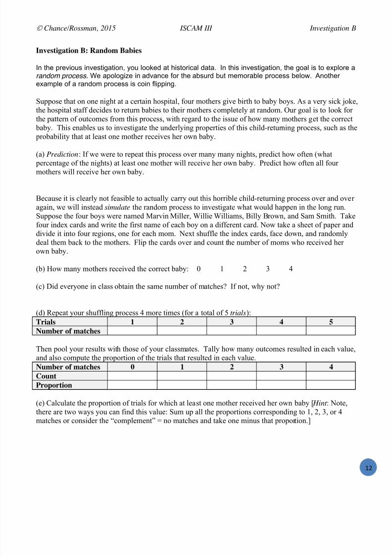
(a) Prediction : If we were to repeat this process over many many nights, predict how often (what percentage of the nights) at least one mother will receive her own baby. Predict how often all fourmothers will receive her own baby.
Because it is clearly not feasible to actually carry out this horrible child-returning process over and overagain, we will instead simulate the random process to investigate what would happen in the long run.Suppose the four boys were named Marvin Miller, Willie Williams, Billy Brown, and Sam Smith. Takefour index cards and write the first name of each boy on a different card. Now take a sheet of paper anddivide it into four regions, one for each mom. Next shuffle the index cards, face down, and randomlydeal them back to the mothers. Flip the cards over and count the number of moms who received herown baby.
(b) How many mothers received the correct baby: 0 1 2 3 4
(c) Did everyone in class obtain the same number of matches? If not, why not?
(d) Repeat your shuffling process 4 more times (for a total of 5 trials ):Trials 1 2 3 4 5Number of matches
Then pool your results with those of your classmates. Tally how many outcomes resulted in each value,and also compute the proportion of the trials that resulted in each value.Number of matches 0 1 2 3 4CountProportion
(e) Calculate the proportion of trials for which at least one mother received her own baby [ Hint : Note,there are two ways you can find this value: Sum up all the proportions corresponding to 1, 2, 3, or 4matches or consider the “complement” = no matches and take one minus that propor tion.]

7/25/2019 Text: Investigating Statistical Concepts, Applications, and Methods
http://slidepdf.com/reader/full/text-investigating-statistical-concepts-applications-and-methods 14/428
Chance/Rossman, 2015 ISCAM III Investigation B
W#
(f) The proportion you have calculated is an estimate of how often this “event” happens in the long run.How does this proportion compare to your prediction in (a)?
(g) How could we improve our estimate of how often this event happens?
08;4$"+8'* <*"$6,8,Open the Random Babies applet and press Randomize .
Notice that the applet randomly returns babies to mothers anddetermines how many babies are returned to the correct home(by matching diaper colors). The applet also counts andgraphs the resulting number of matches. Uncheck theAnimate box and press Randomize a few more times. You
should see the results accumulate in the table and thehistogram. Click on the bar representing the outcome of zeromothers receiving the correct baby. This shows you a “time
plot” of the proportion of trials with 0 matches vs. the numberof trials. Set the Number of trials to 100 and pressRandomize a few times, noticing how the behavior of thisgraph changes.
(h) Describe what you learn about how the (cumulative) proportion of trials that result in zero matcheschanges as you simulate more and more trials of this process.
Definition : A random process generates observations according to a random mechanism, like a cointoss. Whereas we can’t predict each individual outcome with certainty, we do expect to see a long -run
pattern to the results. The probability of a random event occurring is the long-run proportion (orrelative frequency) of times that the event would occur if the random process were repeated over andover under identical conditions. You can approximate a probability by simulating (i.e., artificiallyrecreating) the process many times. Simulation leads to an empirical estimate of the probability, which
is the proportion of times that the event occurs in the simulated repetitions of the random process.Increasing the number of repetitions generally results in more accurate estimates of the long-run probabilities.
(i) After at least 1000 trials, complete the table below.Number of matches 0 1 2 3 4
Proportion
7/25/2019 Text: Investigating Statistical Concepts, Applications, and Methods
http://slidepdf.com/reader/full/text-investigating-statistical-concepts-applications-and-methods 15/428
Chance/Rossman, 2015 ISCAM III Investigation B
W
(j) Based on your answer to (i), what is your estimate for the probability that at least one mother receivesher own baby? Do all of your classmates obtain the same estimate?
(k) Consider the table of Cumulative Results in the applet. One value for the number of matches is fairlyunlikely, but does occur once in a while. Which outcome is this?
(l) One outcome is actually impossible to occur. Which outcome is this? Explain why it is impossible.
(m) Calculate the average number of matches for your 1000 (or however many you performed) trials.[ Hint : Use a weighted average ( xi f i)/ N where xi is the number of matches and f i is the correspondingfrequency, and N is the number of repetitions you simulated.]
(n) Select the Average radio button above the time plot. Describe the behavior of this graph andcomment on what it reveals about the behavior of the average number of matches over many trials.
/A"7+ B"+=%;"+87"$ <*"$6,8,One disadvantage to using simulation to estimate a probability like this is that everyone will potentiallyobtain a different estimate. Even with a very large number of trials, your result will still only be anestimate of the actual long-run probability. For this particular scenario however, we can determine exacttheoretical probabilities.
First, let’s list out all possible outcomes for returning four babies to their mothers at random. We can
organize our work by letting 1234 represent the outcome where the first baby went to the first mother,the second baby to the second mother, the third baby to the third mother, and the fourth baby to thefourth mother. In this scenario, all four mothers get the correct baby. As another example, 1243 meansthat the first two mothers get the right baby, but the third and fourth mothers have their babies switched.
Definition: A sample space is a list of all possible outcomes of a random process.
All of the possible outcomes are listed below:

7/25/2019 Text: Investigating Statistical Concepts, Applications, and Methods
http://slidepdf.com/reader/full/text-investigating-statistical-concepts-applications-and-methods 16/428
Chance/Rossman, 2015 ISCAM III Investigation B
WR
Sample Space:1234 1243 1324 1342 1423 14322134 2143 2314 2341 2413 24313124 3142 3214 3241 3412 34214123 4132 4213 4231 4312 4321
In this case, returning the babies to the mothers completely at random implies that the outcomes in oursample space are equally likely to occur ( outcome probability = 1 / number of possible outcomes ).
(o) How many different outcomes are there for returning four babies to their mothers? What is eachoutcome ’s probability of occurring for any trial?
You could have determined the number of possible outcomes without having to list them first. For thefirst mother to receive a baby, she could receive any one of the four babies. Then there are three babies
to choose from in giving a baby to the second mother. The third mother receives one of the tworemaining babies and then the last baby goes to the fourth mother. Because the number of possibilities atone stage of this process does not depend on the outcome (which baby) of earlier stages, the totalnumber of possibilities is the product 1234 = 24. This is also known as !4 , read “4 factorial.”Because the above outcomes are equally likely, the probability of any one of the above outcomesoccurring is 1/24. Although these 24 outcomes are equally likely, we were more interested above in the
probability of 0 matches, 1 match, etc.
Definition: A random variable maps each possible outcome of the random process (the sample space) to a numerical value. We can then talk about the probability distribution of the random variable.These random variables are usually denoted by capital roman letters, e.g., X , Y . A random variable is
discrete if you can list each individual value that can be observed for the random variable.(p) For each of the above outcomes, indicate (next to the outcome above) how many mothers get thecorrect baby. [ Hint : For outcome 1243, mothers one and two receive their own babies so the value of thenumber of correct matches is 2.]
(q) In how many of the outcomes did zero mothers receive the correct baby?
Probability Rule: When the outcomes in the sample space are equally likely, the probability of anyone of a set of outcomes (an event) occurring is the number of outcomes in that set divided by the totalnumber of outcomes in the sample space.
(r) To calculate the exact probability of 0 matches, divide the number of outcomes with 0 matches by thetotal number of possible outcomes. How does this result compare to your estimate from the simulation?
P( X = 0) = Comparison:

7/25/2019 Text: Investigating Statistical Concepts, Applications, and Methods
http://slidepdf.com/reader/full/text-investigating-statistical-concepts-applications-and-methods 17/428
Chance/Rossman, 2015 ISCAM III Investigation B
W
(s) Use this method to determine the exact probabilities for each possible value for the number ofmatches. Express these probabilities as fractions and as decimals in the table below.
Probability Distribution for # of correct matches: # matches 0 1 2 3 4
Probability(fraction)Probability(decimal)
How do these theoretical probabilities compare to the empirical estimates you found in the simulation(question (i))?
(t) What is the sum of these five probabilities? Why does this make sense?
(u) What is the probability that at least one mother receives the correct baby? [ Hint : Determine this twodifferent ways: first by adding the probabilities of the corresponding values, and then by taking oneminus the probability that this event does not happen.] How does this compare to the simulation results?
Probability rules: The sum of the probabilities for all possible outcomes equals one.
Complement rule : The probability of an event happening is one minus the probability of the eventnot happening. Addition rule for disjoint events : The probability of at least one of several events is the sum of the
probabilities of those events as long as there are no outcomes in common across the events (i.e.,the events are mutually exclusive or disjoint ).
We can also consider the expected value of the number of matches, which is interpreted as the long-runaverage value of the random variable. For a discrete random variable we can calculate the expectedvalue of the random variable X by again employing the idea of a weighted average of the different
possible values of the random variable, but now the “weights” will be given by the probabilities of thosevalues:
E (X) = values
poss ibleallvalueof y probabilit value )()(
(v) Calculate the expected value of the number of matches. Comment on how it compares to theaverage value you obtained in the simulation.

7/25/2019 Text: Investigating Statistical Concepts, Applications, and Methods
http://slidepdf.com/reader/full/text-investigating-statistical-concepts-applications-and-methods 18/428
Chance/Rossman, 2015 ISCAM III Investigation B
WT
(w) Is the expected value for the number of matches equal to the most probable outcome? If not, explainwhat is meant by an “expected” value.
Notice that if we wanted to compute the average number of matches, say after 1000 trials, we wouldlook at a weighted average:
1000
4)4(#2)2(#1)1(#0)0(#...
100002101 sof sof sof sof
x
But from the results we saw above, each term (# of)/1000 terms converges to the probability of thatoutcome as we increase the number of repetitions, giving us the above formula for E ( X ). So we willinterpret the expected value as the long-run average of the outcomes.
Another property of a random variable is its variance . This measures how variable the values of therandom variable will be. For a discrete random variable we can again use a type of weighted average,
based on the probabilities of each value and the squared distances between the possible values of therandom variable and the expected value.
V(X) = values
pos sibleall
valueof y probabilit X E value )())(( 2
(x) Calculate the variance of the number of matches. Also take the square root to calculate the standarddeviation SD(X).
V(X) = SD(X) =
We will interpret this standard deviation similarly to how we did in Investigation A: how far the
outcomes tend to be from the expected value. Here we are talking in terms of the probability model; inInvestigation A we were talking in terms of the historical data.
(y) Confirm that the value of the standard deviation you calculating makes sense considering the possible outcomes for the random variable.
Discussion : Notice that we have used two methods to answer questions about this random process: Simulation – running the process under identical conditions a large number of times and seeing
how often different outcomes occur Exact mathematical calculations using basic rules of probability and countingThis approach of looking at the analysis using both simulation and exact approaches will be a theme inthis course. We will also consider some approximate mathematical models as well. You should considerthese multiple approaches as a way to assess the appropriateness of each method. You should also beaware of situations where one method may be preferable to another and why.

7/25/2019 Text: Investigating Statistical Concepts, Applications, and Methods
http://slidepdf.com/reader/full/text-investigating-statistical-concepts-applications-and-methods 19/428
Chance/Rossman, 2015 ISCAM III Investigation B
W
9:"7+87% 9:'#$%; CD<Suppose three executives (Annette, Barb, and Carlos) drop their cell phones in an elevator and blindly
pick them back up at random.(a) Write out the sample space using ABC notation for the outcomes.(b) Carry out the exact analysis to determine how the probability of at least one executive receiving his
or her own phone.(c) Calculate the expected number of matches for 3 executives. How does this compare to the case with4 mothers?(d) Use the Random Babies applet to check your results.
9:"7+87% 9:'#$%; CDCReconsider the Random Babies. Now suppose there were 8 mothers involved in this random process.(a) Calculate the (exact) probability that all 8 mothers receive the correct baby. [ Hint : First determinehow many possible outcomes there are for returning 8 babies to their mothers.](b) Calculate the probability that exactly 7 mothers receive the correct baby.(c) Using the Random Babies applet, approximate the probability that at least one of the 8 mothersreceives the correct baby. How does your approximation compare to the probability of this event with 4mothers?(d) Using the Random Babies applet, approximate the expected value for how many of the eight motherswill receive the correct baby. How does your approximation compare to the situation with 4 mothers?

7/25/2019 Text: Investigating Statistical Concepts, Applications, and Methods
http://slidepdf.com/reader/full/text-investigating-statistical-concepts-applications-and-methods 20/428
Chance/Rossman, 2015 ISCAM III Chapter 1
WV
CHAPTER 1: ANALYZING ONE CATEGORICAL VARIABLE
In this chapter, you will begin to analyze results from statistical studies and focus on the process ofstatistical inference. In particular, you will learn how to assess evidence against a particular claim abouta random process.
Section 1: Analyzing a process probabilityInvestigation 1.1: Friend or foe Inference for a proportionProbability Exploration: Mathematical ModelProbability Detour: Binomial Random VariablesInvestigation 1.2: Do names match faces Bar graph, hypotheses, binomial test (technology)Investigation 1.3: Heart transplant mortality Factors affecting p-valueInvestigation 1.4: Kissing the right way Two-sided p-valuesInvestigation 1.5: Kissing the right way (cont.) Interval of plausible valuesInvestigation 1.6: Improved baseball player Types of error and powerProbability Exploration: Exact Binomial Power Calculations
Section 2: Normal approximations for sample proportionsInvestigation 1.7: Reese’s pieces Normal model, Central Limit TheoremProbability Detour: Normal Random VariablesInvestigation 1.8: Is ESP real? Normal probabilities, z-scoreInvestigation 1.9: Halloween treat choices Test statistic, continuity correctionInvestigation 1.10: Kissing the right way (cont.) z-interval, confidence levelInvestigation 1.11: Heart transplant mortality (cont.) Plus Four/Adjusted Wald
Section 3: Sampling from a finite populationInvestigation 1.12: Sampling words Biased and random samplingInvestigation 1.13: Literary Digest Issues in samplingInvestigation 1.14: Sampling words (cont.) Central Limit Theorem for p
ˆ
Investigation 1.15: Freshmen Voting Patterns – Nonsampling errors, hypergeometric distributionProbability Detour: Hypergeometric Random VariablesInvestigation 1.16: Teen hearing loss One sample z-proceduresInvestigation 1.17: Cat households Practical significanceInvestigation 1.18: Female senators Cautions in inference
Example 1.1: Predicting Elections from Faces Example 1.2: Cola Discrimination
Example 1.3: Seat Belt Usage
Appendix: Stratified random sampling
! " # $ % & ' ( ) & ' " ( + & ) & ' % & ' , ) - . / " , $ 0 & % 1 2 0 0 - ' , ) & ' / " % 1 ) " 3 4 $ & 5 / 3 %

7/25/2019 Text: Investigating Statistical Concepts, Applications, and Methods
http://slidepdf.com/reader/full/text-investigating-statistical-concepts-applications-and-methods 21/428

7/25/2019 Text: Investigating Statistical Concepts, Applications, and Methods
http://slidepdf.com/reader/full/text-investigating-statistical-concepts-applications-and-methods 22/428
Chance/Rossman, 2015 ISCAM III Investigation 1.1
!W
We can place these explanations into two main categories:(1) There is something to the theory that infants are genuinely more likely to pick the helper toy (for
some reason).(2) Infants choose randomly and we happened to get “lucky” and find most infants picking the helper
toy in our study.
(c) Why are we not considering something like color of the helper toy as a possible explanation?
(d) So for the two explanations we are still considering, how might you choose between them? In particular, how might you convince someone that option (2) is not plausible for this study?
Discussion : As you saw with the Random Babies, we can simulate the outcomes of a random process tohelp use determine which types of outcomes are more or less likely to occur. In this case, we can easilysimulate what “could have happened” if the infants are randomly guessing. In other words, our analysisis going to assume the researchers’ conjecture is wrong (for the moment) and that infants really are just
blindly picking one toy or the other without any regard for whether it was the helper toy or the hinderer.
(e) Suggest a method for carrying out this simulation of infants picking equally between the two toys.
(f) Explain why looking at such “could have been” results will be useful to us.
Discussion: We will call the assumption that these infants have no genuine preference between the toysthe null model . Performing lots of repetitions under this model will enable us to see the pattern of results(number who choose the helper toy) when we know the infants have no preference . Examining this nulldistribution will in turn help us to determine how unusual it is to get 14 infants picking the helper toywhere there is no genuine preference. If the answer is that that the result observed by the researchers (14of 16 choosing the helper toy) would be very surprising for infants who had no real preference, then wewould have strong evidence to conclude that infants really do prefer the helper. Why? Becauseotherwise, we would have to believe a very rare coincidence just happened to occur in this study.Summing up: An observed outcome that would rarely happen if a claim were true provides strongevidence that the claim is not true.

7/25/2019 Text: Investigating Statistical Concepts, Applications, and Methods
http://slidepdf.com/reader/full/text-investigating-statistical-concepts-applications-and-methods 23/428
Chance/Rossman, 2015 ISCAM III Investigation 1.1
!
08;4$"+8'* (g) Flip a coin 16 times, representing the 16 infants in the study (one trial or repetition from this random
process). Let a result of heads mean that the infant chooses the helper toy, tails for the hinderer toy.Tally the results below and count how many of the 16 chose the helper toy:
“Could have been” distribution
Heads (helper toy) Tails (hinderer toy)
Total number of heads in 16 tosses:
(h) Repeat this two more times. Keep track of how many infants, out of the 16, choose the helper.Record this number for all three of your repetitions (including the one from the previous question):
Repetition # 1 2 3Number of (simulated) infants who chose helper
(i) Combine your simulation results for each repetition with your classmates on the scale below. Createa dotplot by placing a dot above the numerical result found by each person.
(j) Did everyone get the same number of heads every time? What is an average or typical number ofheads? Is this what you expected? Explain.
(k) How is it looking so far – is the actual study result (14 picking the helper toy) consistent with theoutcomes that could have happened under the null model? Which explanation (1) or (2) do you think ismore plausible based on this null distribution? Explain your reasoning.
7/25/2019 Text: Investigating Statistical Concepts, Applications, and Methods
http://slidepdf.com/reader/full/text-investigating-statistical-concepts-applications-and-methods 24/428
Chance/Rossman, 2015 ISCAM III Investigation 1.1
!#
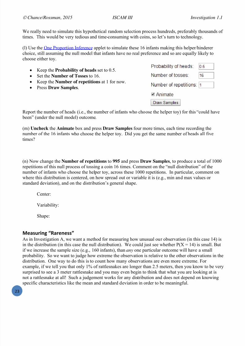
We really need to simulate this hypothetical random selection process hundreds, preferably thousands oftimes. This would be very tedious and time- consuming with coins, so let’s turn to technology.
(l) Use the One Proportion Inference applet to simulate these 16 infants making this helper/hindererchoice, still assuming the null model that infants have no real preference and so are equally likely to
choose either toy.
Keep the Probability of heads set to 0.5. Set the Number of Tosses to 16. Keep the Number of repetitions at 1 for now. Press Draw Samples .
Report the number of heads (i.e., the number of infants who choose the helper toy) for this “could have been” (under the null model) outcome .
(m) Uncheck the Animate box and press Draw Samples four more times, each time recording thenumber of the 16 infants who choose the helper toy. Did you get the same number of heads all fivetimes?
(n) Now change the Number of repetitions to 995 and press Draw Samples , to produce a total of 1000repetitions of this null process of tossing a coin 16 times. Comment on the “null distribution ” of thenumber of infants who choose the helper toy, across these 1000 repetitions. In particular, comment onwhere this distribution is centered, on how spread out or variable it is (e.g., min and max values orstandard deviation ), and on the distribution’s general shape.
Center:
Variability:
Shape:
Measuring “ @":%*%,,” As in Investigation A, we want a method for measuring how unusual our observation (in this case 14) isin the distribution (in this case the null distribution). We could just see whether P(X = 14) is small. Butif we increase the sample size (e.g., 160 infants), than any one particular outcome will have a small
probability. So we want to judge how extreme the observation is relative to the other observations in thedistribution. One way to do this is to count how many observations are even more extreme. Forexample, if we tell you that only 1% of rattlesnakes are longer than 2.5 meters, then you know to be verysurprised to see a 3 meter rattlesnake and you may even begin to think that what you are looking at isnot a rattlesnake at all! Such a judgement works for any distribution and does not depend on knowingspecific characteristics like the mean and standard deviation in order to be meaningful.

7/25/2019 Text: Investigating Statistical Concepts, Applications, and Methods
http://slidepdf.com/reader/full/text-investigating-statistical-concepts-applications-and-methods 25/428
Chance/Rossman, 2015 ISCAM III Investigation 1.1
!
(o) Report how many and what proportion of these 1000 samples produced 14 or more infants choosingthe helper toy:
Enter 14 in the As extreme as box Number of repetitions: Press the Count button. Proportion of repetitions:
(p) Did everyone in your class get the same proportion? Does this surprise you?
(q) Based on the proportion you found in (o), would you say that the actual result obtained by theresearchers is very rare, somewhat rare, or not very rare, under the null model that infants have no
preference and so choose blindly? Circle one of these three:
Very rare Somewhat rare Not very rare
(r) So, based on your simulation results, would you say that the researchers have very strong evidencethat these infants’ selection process is not like flipping a coin, and instead the more plausible
explanation is that these infants do have a preference for the helper toy?
!%:;8*'$'>6 2%+'4:The long-run proportion of times that an event happens when its random process is repeatedindefinitely is called the probability of the event. We can approximate a probability empirically bysimulating the random process a large number of times and determining the proportion of times that
the event happens.
More specifically, the probability that the random process specified by the null model would produceresults as or more extreme as the actual study result is called a p-value . Our analysis aboveapproximated this p- value by simulating the infants’ random selection process a large number of timesand finding how often we obtained results at least as extreme as the actual data. You can obtain betterand better approximations of this p-value by using more and more repetitions in your simulation.
A small p-value indicates that the observed data would be surprising to occur through the random process alone, if the null model were true. Such a result is said to be statistically significant , providingevidence against the null model (so we don’t believe the discrepancy arose just by chance but instead
reflects a genuine tendency). The smaller the p-value, the stronger the evidence against the nullmodel. There are no hard-and-fast cut-off values for gauging the smallness of a p-value, but generallyspeaking:
A p-value above 0.10 constitutes little or no evidence against the null model. A p-value below 0.10 but above 0.05 constitutes moderate evidence against the null model. A p-value below 0.05 but above 0.01 constitutes strong evidence against the null model. A p-value below 0.01 constitutes very strong evidence against the null model.

7/25/2019 Text: Investigating Statistical Concepts, Applications, and Methods
http://slidepdf.com/reader/full/text-investigating-statistical-concepts-applications-and-methods 26/428
Chance/Rossman, 2015 ISCAM III Investigation 1.1
!R
07'?% '( )'*7$4,8'*,What bottom line does our analysis lead to? Do infants in general show a genuine preference for the“helper” toy over the “hinderer” one? Well, there are rarely definitive answers when working with realdata, but our analysis reveals that the study provides strong evidence that these infants are not behavingas if they were tossing coins. That is, we have strong evidence that the probability of choosing the
helper toy in this process is greater than 0.5. Because the researchers controlled for other possibleexplanations for the observed preference, we will conclude that there is convincing evidence that infantsreally do have a preference.
(s) Can we reasonably claim that it was the actions of the objects in the videos that influenced theinfants’ choices or is “random luck” still a plausible (believable) explanation? Explain.
(t) Can we reasonably extend this conclusion beyond the 16 infants in the study? Explain. [Note: Wewill discuss this issue in more detail later. What does your intuition tell you for now?]
0+456 )'*7$4,8'*,If we assume the infants choose between the two toys with equal probability, than we can modelthis random process with coin tossing. Approximating the p-value , we found that getting 14 ormore infants choosing the helper toy, if the infants are choosing at random, is very unlikely bychance alone. This means that the data provide very strong statistical evidence to reject this “no
preference” model and conclude that these infants’ choices are actually governed by a processwhere there is a genuine preference for the helper toy (or at least that it’s more complicated thaneach infant flipping a coin to decide). Of course, the researchers really care about whetherinfants in general (not just the 16 in this study) have such a preference. Extending the results toa larger group of infants depends on whether it’s reasonable to believe that the infants in thisstudy are representative of a larger group of infants on this question. We cannot make this
judgment without knowing more about how these infants were selected. However, you may be
able to argue that these 16 infants’ choices are representative of the larger process of viewing thevideos and selecting a toy to play with.

7/25/2019 Text: Investigating Statistical Concepts, Applications, and Methods
http://slidepdf.com/reader/full/text-investigating-statistical-concepts-applications-and-methods 27/428
Chance/Rossman, 2015 ISCAM III Investigation 1.1
!
04;;":6Let’s take a step back and consider the reasoning process and analysis strategy that we have employedhere. Our reasoning process has been to start by supposing that infants in general have no genuine
preference between the two toys (our null model), and then ask what results we expect to see under thisnull model (the null distribution) and whether the results observed by the researchers would be unlikely
to have occurred just by random chance assuming this null model. To recap: We summarize the study results with one number, called a statistic. Assume the null model is true, and simulate the random process under this model, producing
data that “could have been” seen in the study if the null model were true. Calculate the value ofthe statistic from these “could have been” data. Then repeat this simulation a large number oftimes, generating the “null distribution” of the values of the statistic.
Evaluate the strength of evidence against the null model by considering how extreme theobserved value of the statistic is in the null distribution. If the observed value of the statistic fallsin the tail of the null distribution, then reject the null model as not plausible. Otherwise, considerthe null model to be plausible (but not necessarily true, because other models might also be
plausible).
In this study, our statistic is the number (or the proportion) of the 16 infants who chose the helper toy.We assume that infants do not prefer either toy (the null model) and simulate the hypothetical randomselection process a large number of times under this assumption. We noted that our actual statistic (14of 16 choosing the h elper toy) is in the upper tail of the simulated null distribution. Such a “tail result”indicates that the data observed by the researchers would be very surprising if the null model were true,giving us strong evidence against the null model. So instead of thinking the researchers just got thatlucky that day, a more reasonable conclusion would be to “reject that null model.” Therefore, this study
provides very strong evidence to conclude that these infants really do prefer the helper toy and were notessentially flipping a coin in making their selections.
Important note: If you do not obtain a small p-value, all you can conclude is that the null model is
plausible for the overall process, but that other values could be plausible for the long-run probability aswell. You have in no way proven that the hypothesized value is correct, just that you don’t haveconvincing evidence it is false. In such a case, statisticians are very careful to say they fail to reject thenull hypothesis, rather than saying an ything that conveys they “accept” the null hypothesis.
9:"7+87% 9:'#$%; HDH<(a) In a second experiment, the same events were repeated but the object climbing the hill no longer hadthe googly eyes attached. The researchers wanted to see whether the preference was made based on asocial evaluation more than a perceptual preference. Suppose they found ten of sixteen 10-month-olds
chose the helper in this study. If you were to use a coin to carry out a simulation analysis to evaluatethese results: how many times would you flip the coin? How many times would you repeat the process?You would then determine the proportion that are ( choose one: ,, ) (choose one: 8, 10, 14, 16, 1000).(b) Use the One Proportion Inference applet to approximate the p-value and compare to the p-value ofthe original study. Explain why this comparison makes intuitive sense. [Be sure to explain what valuesyou input into the applet.](c) What does the statistical significance of the first study and not of the second tell the researchers?

7/25/2019 Text: Investigating Statistical Concepts, Applications, and Methods
http://slidepdf.com/reader/full/text-investigating-statistical-concepts-applications-and-methods 28/428
Chance/Rossman, 2015 ISCAM III Probability Detour
!T
9:'#"#8$8+6 /A?$':"+8'*I B"+=%;"+87"$ B'5%$ (a) Did everyone in your class obtain the same approximate p-value from their simulation of 1000repetitions? If not, are these approximate p-values all fairly close to each other?
Simulating 1000 repetitions is generally good enough to produce a reasonable approximation for theexact p-value. But in this case you can also determine this probability (p-value) exactly (as if the
process were repeated infinitely often) using what are called binomial probabilities. The probability ofobtaining k successes in a sequence of n trials with success probability on each trial is:
P(X = k ) = k nk
k
n
1 where)!(!
!k nk
nk
n
Here X represents a random variable which counts the number of successes in n trials. The short-handnotation for saying X follows a binomial distribution is X Bin( n, ). (See Probability Detour below.)
Use this expression to determine the exact probability of obtaining 14 or more successes (infants whochoose the helper toy) in a sequence of 16 trials, under the null model that the underlying success probability on each trial, , is 0.5:
(b) First determine the probability of exactly 14 successes, so k = 14, n = 16, and = 0.5:
P(X = 14) =
(c) Repeat (b) to find the (exact) probability of obtaining 15 successes. Then repeat to find the probability of obtaining 16 successes.
P(X = 15) = P(X = 16) =(d) Add these three probabilities to determine the (exact) p-value for 14 or more successes. Did theapproximate p- value from your simulation come close to this value? Which value is “better”?
P(X 14) =
Comparison:
The exact p-value (to four decimal places, see Technology Detour) turns out to be 0.0021. We can
interpret this by saying that if infants really had no preference and so were randomly choosing equally between the two toys, there’s only about a 0.21% chance that 14 or more of the 16 infants would havechosen the helper toy. [Or, similar to what we saw in the simulation, such a result would only happenroughly twice in 1,000 samples.] Because this probability is quite small, the researchers’ data providevery strong evidence that having 14 of the infants pick the helper toy did not occur by chance alone andtherefore strong evidence that infants in general really do have a preference for the nice (helper) toy.
7/25/2019 Text: Investigating Statistical Concepts, Applications, and Methods
http://slidepdf.com/reader/full/text-investigating-statistical-concepts-applications-and-methods 29/428
Chance/Rossman, 2015 ISCAM III Probability Detour
!
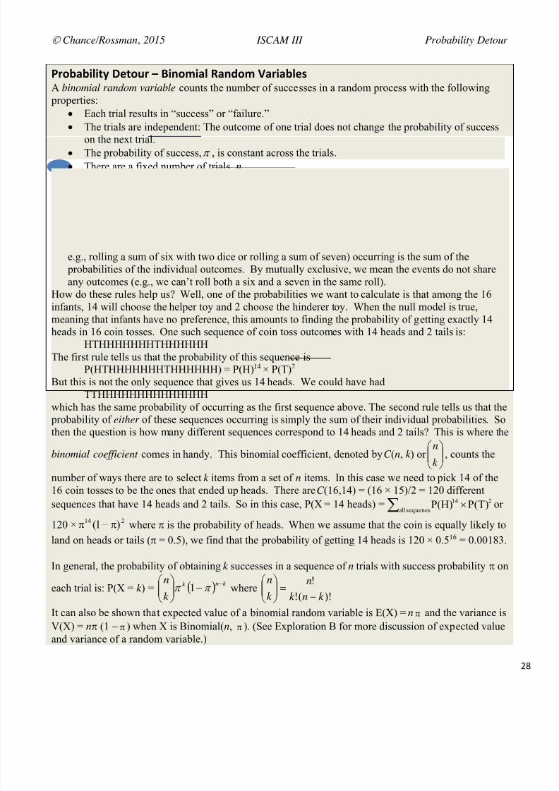
9:'#"#8$8+6 2%+'4: – C8*';8"$ @"*5'; J":8"#$%, A binomial random variable counts the number of successes in a random process with the following
properties: Each trial results in “success” or “failure.” The trials are independent: The outcome of one trial does not change the probability of success
on the next trial. The probability of success, , is constant across the trials. There are a fixed number of trials, n.
If X counts the number of successes, then we can say X Binomial ( n, ).In this case, the probability calculation follows from several simple probability rules: When the trials are independent (the outcome on one trial does not affect the probability of success
on another trial), the probability of several outcomes occurring simultaneously is the product of the probabilities of the individual outcomes.
The probability of one of several mutually exclusive events (eve nts that can’t occur simultaneously,e.g., rolling a sum of six with two dice or rolling a sum of seven) occurring is the sum of the
probabilities of the individual outcomes. By mutually exclusive, we mean the events do not shareany outcomes (e.g., we ca n’t roll both a six and a seven in the same roll).
How do these rules help us? Well, one of the probabilities we want to calculate is that among the 16infants, 14 will choose the helper toy and 2 choose the hinderer toy. When the null model is true,meaning that infants have no preference, this amounts to finding the probability of getting exactly 14heads in 16 coin tosses. One such sequence of coin toss outcomes with 14 heads and 2 tails is:
HTHHHHHHHTHHHHHHThe first rule tells us that the probability of this sequence is
P(HTHHHHHHHTHHHHHH) = P(H) 14 ! P(T) 2
But this is not the only sequence that gives us 14 heads. We could have hadTTHHHHHHHHHHHHHH
which has the same probability of occurring as the first sequence above. The second rule tells us that the probability of either of these sequences occurring is simply the sum of their individual probabilities. Sothen the question is how many different sequences correspond to 14 heads and 2 tails? This is where the
binomial coefficient comes in handy. This binomial coefficient, denoted by C (n, k ) or
k
n, counts the
number of ways there are to select k items from a set of n items. In this case we need to pick 14 of the16 coin tosses to be the ones that ended up heads. There are C (16,14) = (16 ! 15)/2 = 120 differentsequences that have 14 heads and 2 tails. So in this case, P(X = 14 heads) =
sequenesall214 P(T)P(H) or
120 ! 214 )1( where is the probability of heads. When we assume that the coin is equally likely toland on heads or tails ( = 0.5), we find that the probability of getting 14 heads is 120 ! 0.516 = 0.00183.
In general, the probability of obtaining k successes in a sequence of n trials with success probability on
each trial is: P(X = k ) = k nk
k
n
1 where)!(!
!k nk
nk
n
It can also be shown that expected value of a binomial random variable is E(X) = n and the variance isV(X) = n (1 ) when X is Binomial( n, ). (See Exploration B for more discussion of expected valueand variance of a random variable.)

7/25/2019 Text: Investigating Statistical Concepts, Applications, and Methods
http://slidepdf.com/reader/full/text-investigating-statistical-concepts-applications-and-methods 30/428
Chance/Rossman, 2015 ISCAM III Probability Detour
!V
<* <$+%:*"+8F% B%",4:% '( @":%*%,,
As an alternative to the p-value, another measure of where an observation falls in a distribution is “howmany standard deviations” it is from the mean of the distribution . But if our data is “helper” or“hinderer,” how do we calculate the standard deviation? Recall that the standard deviation measures the
variability or spread of a distribution from the mean and refers to how clustered together or consistent the values are.
Suppose we had “coded” each infant’s outcome as 0 or 1: ID Infant
choiceCodedchoice
ID Infantchoice
Codedchoice
ID Infantchoice
Codedchoice
ID Infantchoice
Codedchoice
1 Helper 1 5 Helper 1 9 Helper 1 13 Helper 12 Helper 1 6 Helper 1 10 Helper 1 14 Helper 13 Hinderer 0 7 Hinderer 0 11 Helper 1 15 Helper 14 Helper 1 8 Helper 1 12 Helper 1 16 Helper 1
(e) If we treat the data numerically in this manner, what is the mean or average of these 16 values?
(f) Use technology (e.g., Descriptive Statistics applet) to calculate the standard deviation of these 16values.
Discussion : We are again looking at the “ typical deviation” from the mean. With 14 ones and twozeros, the mean is 14/16 = 0.875 (the same as the sample proportion). The squared deviations from thismean are (1 – 0.875) 2 and there are 14 of these (so most of the data values are pretty close to the mean)
and (0 – 0.875) 2 and there are two of these. So summing these squared deviations and dividing by n – 1= 15, we get a variance of 1.75/15 0.1167. Taking the square root of the variance gives us the standarddeviation.
(g) Take the square root of this variance, how does it compare to the standard deviation calculated in (f)?
(h) Suppose 8 infants had chosen the helper toy and 8 infants had chosen the hinderer toy, sketch the“dotplot” in this case.
(i) Would you consider those results more, or less, or equally “consistent” than the actual results?

7/25/2019 Text: Investigating Statistical Concepts, Applications, and Methods
http://slidepdf.com/reader/full/text-investigating-statistical-concepts-applications-and-methods 31/428
Chance/Rossman, 2015 ISCAM III Probability Detour
#
(j) Use technology to calculate the standard deviation (or by hand) for this hypothetical 8/8 split. Doesthis confirm your answer to (i)? In other words, which has more variability, the hypothetical data or theactual study? (In other words, in which case would it be easier to predict a future observation?)
(k) Is it possible for a data set of 16 zeros and ones to have a larger standard deviation than in (j)? Whatwould need to be true for the 16 values to have the smallest possible standard deviation (and what is thevalue of the standard deviation in that case)?
Largest: Smallest:
Discussion: If data t end to be far from the average value, then we consider these data to be “lessconsistent” or “more spread out” and we say the data set has “more variability.” It’s critical to keep inmind that variability refers to (horizontal) distances of the data values from the center of the distribution.
If most values are close to the mean, the variability will be small, and so the average deviance from thecenter will be small. If many of the values are far from the mean of the data set, then the variability will be larger, and so the average deviation will be larger. Although it’s actually rather unusual to considervariability when we have only yes/no outcomes (it really doesn’t give us any additional information
beyond the sample proportion), we hope this discussion will help you keep in mind this interpretation ofthe concept of variability and how average deviation from the mean provides a reasonable measure ofvariability.
(l) But in this case, we actually want to know about the variance of our random variable, number ofbabies that choose the helper toy . The Probability Detour for the Binomial distribution tells us thatV(X) = n (1 ) for different repetitions of the random binomial process. For what values of will this
variance be the largest? Smallest? ( Hint : You may want to graph this function for different values of ).
(m) Calculate the standard deviation of this probability model under the null model (assuming =0.50).
(n) Now calculate the number of standard deviations 14 falls from the center of the null distribution.
We still need a way to judge whether your answer to (n) is considered large. We will discuss this inmore detail later, but for now, when we have a fairly symmetric distribution, as your null distributionshould be in this investigation, values larger than 2 or less than 2 are typically considered extreme.
(o) Is your answer to (n) larger than 2? Is this consistent with your p-value for this study? Explain.
7/25/2019 Text: Investigating Statistical Concepts, Applications, and Methods
http://slidepdf.com/reader/full/text-investigating-statistical-concepts-applications-and-methods 32/428
Chance/Rossman, 2015 ISCAM III Technology Detour
#W
9:"7+87% 9:'#$%; HDHC (a) Suppose we thought there was a 60% chance that an infant would choose the helper toy. Explainhow we would change our simulation to represent this null model.(b) Carry out a simulation (e.g., One Proportion Inference applet) to determine whether our observedresult of 14 helper choices by 16 infants is surprising for a process with = 0.60. Report and evaluate
an approximate p-value.(c) How does the distribution of the “number of successes” with = 0.60 compare to when = 0.50?Comment on shape, center, and variability.(d) Determine the exact p-value using the binomial distribution. How does it compare to yoursimulation results?(e) For the binomial model, report the expected value and standard deviation of the number of infantschoosing the helper toy with = 0.60 and n = 16.(f) How many standard deviations is 14 from the expected value for this model? Is it larger or smallerthan what you found in (n) in the previous exploration? Explain why this change makes sense.
7/25/2019 Text: Investigating Statistical Concepts, Applications, and Methods
http://slidepdf.com/reader/full/text-investigating-statistical-concepts-applications-and-methods 33/428
Chance/Rossman, 2015 ISCAM III Technology Detour
#
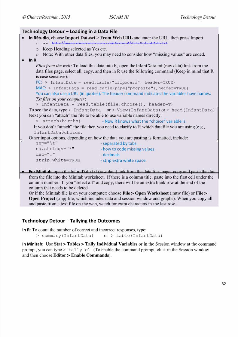
!%7=*'$'>6 2%+'4: – K'"58*> 8* " 2"+" L8$% M* @0+458', choose Import Dataset > From Web URL and enter the URL, then press Import.
C e.g., +%%8?YY<<</51((*&.)+&.),/)1*Y'()&*#Y;&%&[email protected]&.%E&%&/%B% C Keep Heading selected as Yes etc.C Note: With other data files, you may need to consider how “missing values” are coded.
M* @Files from the web: To load this data into R, open the @.9&.%E&%&/%B% (raw data) link from thedata files page, select all, copy, and then in R use the following command (Keep in mind that Ris case sensitive):ON? . Y<GB<7%B7B ! 3;BA=7BL4;&5I4?8LCB3A5Q 6;BA;3!UPJ'*C0N? . Y<GB<7%B7B ! 3;BA=7BL4;&8?8;&58LI8B97;5*Q6;BA;3!UPJ'* D12 )&. &-(1 2(, & Z[\ F'. A21%,(G/ I+, +,&;,5 )1**&.; '.;')&%,( %+, 4&5'&=-,( +&4, .&*,(/Txt files on your computer :. Y<GB<7%B7B ! 3;BA=7BL4;&G?4;=I6CC9;&*Q 6;BA;3!U*
To see the data, type . Y<GB<7%B7B or . V?;>&Y<GB<7%B7B* or . 6;BA&Y<GB<7%B7B* Next you can “attach” the file to be able to use variable names directly:
> B77BI6&L?3769* : Now R k nows what the “choice” variable is If you don’t “attach” the file then you need to clarify to R which datafile you are using (e.g.,Y<GB<7%B7BWI6C?I; .
Other input options, depending on how the data you are pasting is formatted, include:9;8!5Z75 : (,8&5&%,; =6 %&=( <B=973?<D9!5+5 : +1< %1 )1;, *'(('.3 4&-2,(A;I!5=5 : ;,)'*&-(973?8=>6?7;!UPJ' : (%5'8 ,B%5& <+'%, (8&),
L': B8*8+"# , open the @.9&.%E&%&/%B% (raw data) link from the data files page, copy and paste the data
from the file into the Minitab worksheet. If there is a column title, paste into the first cell under thecolumn number. If you “select all” and copy, there will be an extra bl ank row at the end of thecolumn that needs to be deleted.Or if the Minitab file is on your computer: choose File > Open Worksheet (.mtw file) or File >Open Project (.mpj file, which includes data and session window and graphs). When you copy alland paste from a text file on the web, watch for extra characters in the last row.
!%7=*'$'>6 2%+'4: – !"$$68*> +=% -4+7';%,
M* @: To count the number of correct and incorrect responses, type:
. 9200B31&Y<GB<7%B7B* or . 7BL4;&Y<GB<7%B7B*M* B8*8+"#I Use Stat > Tables > Tally Individual Variables or in the Session window at the command
prompt, you can type . 7B441 I, (To enable the command prompt, click in the Session windowand then choose Editor > Enable Commands ).

7/25/2019 Text: Investigating Statistical Concepts, Applications, and Methods
http://slidepdf.com/reader/full/text-investigating-statistical-concepts-applications-and-methods 34/428
Chance/Rossman, 2015 ISCAM III Technology Detour
##
!%7=*'$'>6 2%+'4: – C": N:"?=,
):%"+8*> " C": N:"?= 8* @ O:"G 5"+"P You need to pass the tabled data into the =&58-1% function:
. LB384C7&7BL4;&Y<GB<7%B7B*Q [4BL!5"6C?I;5Q 14BL!5R3;\2;<I15*
You may need to toggle to the R Graphics Window to see the graph window. Now you can use R toexport the graph to a file or you can Copy and Paste or use a screen capture.
):%"+8*> " C": N:"?= 8* @ O,4;;":6 5"+"P If you already (or only) have the summarized data (the number of successes and failures), can type:
> LB384C7&I&,]Q #*Q <B0;9=B3D!I&5T;48;35Q 5T?<A;3;35**
):%"+8*> " C": N:"?= 8* B8*8+"# O:"G 5"+"P Choose Graph > Bar Chart . Press OK (Counts of Unique Values,
Simple).
Specify the column with the categoricalresponses.
Press OK .
):%"+8*> " C": N:"?= 8* B8*8+"# O,4;;":6 5"+"P Put the category names in a second column; put
the number of successes and failures into onecolumn in Minitab.
Choose Graph > Bar Chart . Use the pull- down menu to select “Values from
a Table.” Press OK .
Enter the counts column into the Graphvariables box and the names column into theCategorical variable box.
(Under Chart Options, you can convert to percentages on the vertical axis)
Press OK .
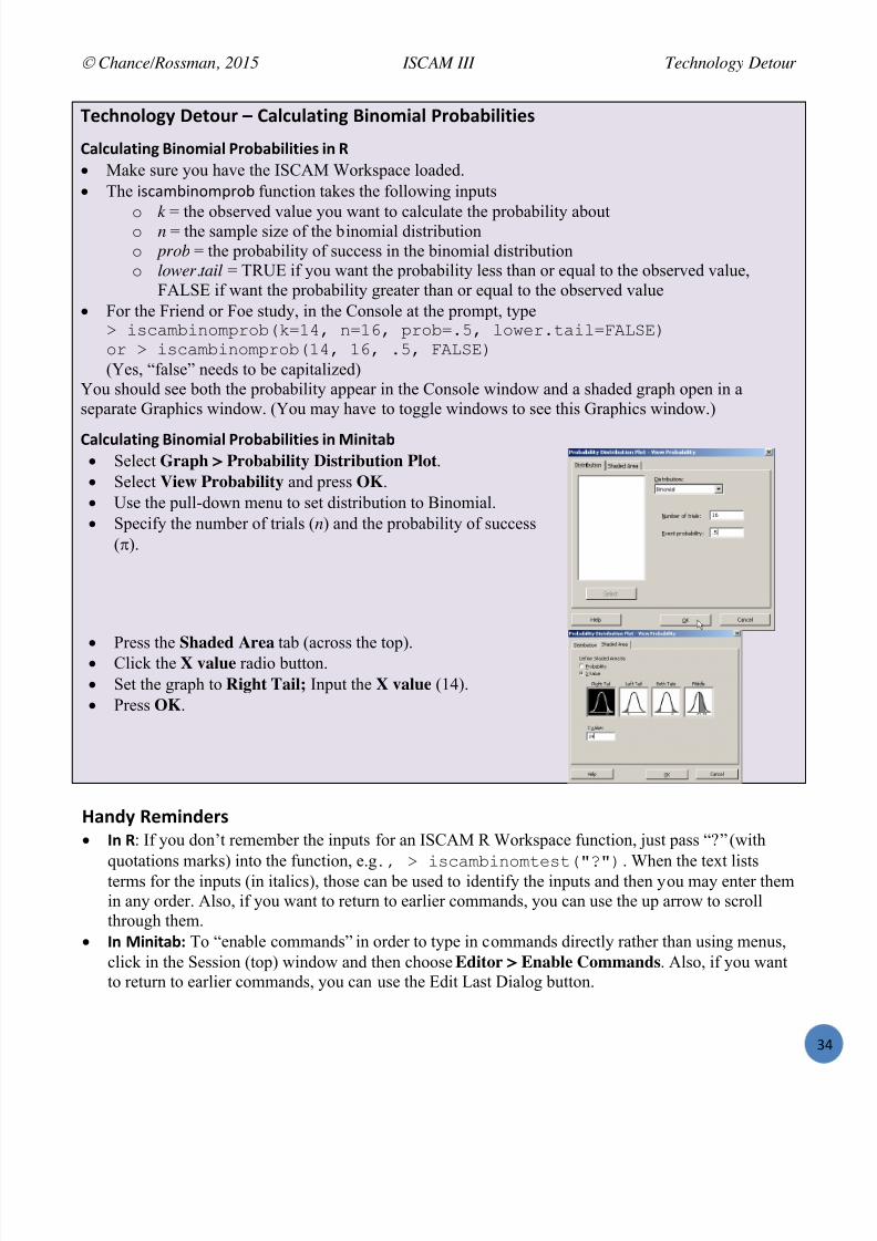
7/25/2019 Text: Investigating Statistical Concepts, Applications, and Methods
http://slidepdf.com/reader/full/text-investigating-statistical-concepts-applications-and-methods 35/428
Chance/Rossman, 2015 ISCAM III Technology Detour
#
!%7=*'$'>6 2%+'4: – )"$74$"+8*> C8*';8"$ 9:'#"#8$8+8%,
)"$74$"+8*> C8*';8"$ 9:'#"#8$8+8%, 8* @ Make sure you have the ISCAM Workspace loaded. The '()&*='.1*851= function takes the following inputs
C k = the observed value you want to calculate the probability aboutC n = the sample size of the binomial distributionC prob = the probability of success in the binomial distributionC lower.tail = TRUE if you want the probability less than or equal to the observed value,
FALSE if want the probability greater than or equal to the observed value For the Friend or Foe study, in the Console at the prompt, type
. ?9IB0L?<C083CL&@!,]Q <!,^Q 83CL!=_Q 4C>;3=7B?4!RSEK'*C3 . ?9IB0L?<C083CL&,]Q ,^Q =_Q RSEK'*(Yes, “false” needs to be capitalized)
You should see both the probability appear in the Console window and a shaded graph open in aseparate Graphics window. (You may have to toggle windows to see this Graphics window.)
)"$74$"+8*> C8*';8"$ 9:'#"#8$8+8%, 8* B8*8+"# Select Graph > Probability Distribution Plot . Select View Probability and press OK . Use the pull-down menu to set distribution to Binomial. Specify the number of trials ( n) and the probability of success
( ).
Press the Shaded Area tab (across the top). Click the X value radio button. Set the graph to Right Tail; Input the X value (14). Press OK .
."*56 @%;8*5%:, M* @: If you don’t remember the inputs for an ISCAM R Workspace function, just pass “?” (with
quotations marks) into the function, e.g= Q . ?9IB0L?<C07;97&5`5*
. When the text liststerms for the inputs (in italics), those can be used to identify the inputs and then you may enter themin any order. Also, if you want to return to earlier commands, you can use the up arrow to scrollthrough them.
M* B8*8+"#I To “enable commands” in order to type in commands directly rather than using menus,click in the Session (top) window and then choose Editor > Enable Commands . Also, if you wantto return to earlier commands, you can use the Edit Last Dialog button.

7/25/2019 Text: Investigating Statistical Concepts, Applications, and Methods
http://slidepdf.com/reader/full/text-investigating-statistical-concepts-applications-and-methods 36/428
Chance/Rossman, 2015 ISCAM III Investigation 1.2
#R
Investigation 1.2: Do Names Match Faces?
A study in Psychonomic Bulletin and Review (Lea, Thomas, Lamkin, & Bell, 2007) presented evidencethat “people use facial prototypes when they encounter different names.” Similar to one of theexperiments they conducted, you will be asked to match photos of two faces to the names Tim and Bob.
The researchers wrote that their participants “overwhelmingly agreed” on which face belonge d to Tim.You will conduct a similar study in class to see whether your class also agrees with which face is Tim’smore than you would expect from random chance (if there is no facial prototyping and people pick aname for the face on the left at random). (Note, you may want to alternate or randomize which face is
placed on the left, which name you mention first, etc.)
(a) Describe in words the null model for this study.
(b) Consider whether we can model this study as a binomial random process. Do you consider the properties necessary for a binomial random variable to be met in this context? What assumptions need to be made? [ Hint : See the Probability Detour box in the previous investigation.]
04;;":8E8*> +=% 2"+" Your instructor will collect and share your class results.(c) How many subjects participated in your study? What proportion of the respondents agreed that theface with the goatee was Tim? Does this appear to be an “overwhelming majority” to you?
(d) Produce a bar graph of the results. Make sure the axes are well-labeled. Can we conclude from thisgraph that people use facial prototyping? Explain.
7/25/2019 Text: Investigating Statistical Concepts, Applications, and Methods
http://slidepdf.com/reader/full/text-investigating-statistical-concepts-applications-and-methods 37/428
Chance/Rossman, 2015 ISCAM III Investigation 1.2
#
!%:;8*'$'>6 2%+'4: To improve our communication about data, we need to define several terms that will be used throughoutthis book.
Definition: The observational units are the people or objects about which data are recorded. A
variable is any characteristic that varies from observational unit to observational unit. A study’ssample size is the number of observational units in the study. In Investigation 1.1, the observational units were the 16 infants. The variable of interest was whichtoy the child chose to play with. Other variables we could have recorded on the infants include age,handedness, and gender.
Definition: We classify the type of variable as categorical (assigning each observational unit to acategory) or quantitative (assigning each observational unit a numerical measurement). A special typeof categorical variable is a binary variable, which has just two possible outcomes. One way to decide between these types is to ask yourself whether or not you can take the average ofthe values. For example, gender is categorical but age is quantita tive. The zip code of the baby’s
home would be categorical even though it is a number, because arithmetic operations like adding oraveraging do not make sense on zip codes. Age can often be treated either way. We will consider itquantitative if the data were recorded in such a way that it makes sense to discuss the average age ofthe employees, but not if they have been grouped into age categories.Also keep in mind that when you have a binary variable, we often (and it may be arbitrarily) defineone outcome to be a “success” (the one we will focus on) and the other to be a “failure.”
Definition: We will also differentiate between a statistic and a parameter . A statistic is a (known)numerical value that summarizes the observed results, whereas a parameter is the same numericalsummary but applied to the underlying random process that generated the data (whose value is usuallyunknown).
In Investigation 1.1, the statistic could be either the number (14) or the proportion (0.875) of infantswho chose the helper toy. The parameter would then be the long-run probability of an infant pickingthe helper toy. (We rejected 0.5 as the value of this parameter, deciding it’s actually larger than 0.50.)With a single categorical variable, we will refer to a sample proportion (a statistic) by the symbol p
ˆ
and a process probability (a parameter) by the symbol .
(e) Define the observational units and variable for this study. Is the variable quantitative or categorical?If categorical, is it binary? If binary, define a success and a failure.
(f) Define a statistic and a parameter for this study (and denote each by the appropriate symbols). Forwhich of these (parameter or statistic) do we know the value, and for which do we not know the value?For the one that we know, report the value as well.
Statistic:
Parameter:

7/25/2019 Text: Investigating Statistical Concepts, Applications, and Methods
http://slidepdf.com/reader/full/text-investigating-statistical-concepts-applications-and-methods 38/428

7/25/2019 Text: Investigating Statistical Concepts, Applications, and Methods
http://slidepdf.com/reader/full/text-investigating-statistical-concepts-applications-and-methods 39/428

7/25/2019 Text: Investigating Statistical Concepts, Applications, and Methods
http://slidepdf.com/reader/full/text-investigating-statistical-concepts-applications-and-methods 40/428
Chance/Rossman, 2015 ISCAM III Investigation 1.2
#V
(m) Would you consider the class results to be statistically significant ? Explain.
)'*7$4,8'*, (n) Based on your calculations, does your class study provide strong evidence that students are likely tomatch the name Tim to the face with the goatee more than we would expect if they are just guessing?
0+456 )'*7$4,8'*,With a small p-value, we would have very strong evidence to reject the null hypothesis and concludethat the students like those in your class have a genuine tendency to identify the “correct” name withthe picture of Tim. Again, we might be cautious in generalizing these results to other names/faces oreven to other subjects identifying the names. We have also assumed that students behave as a
binomial process and all have the same probability of picking Tim (the randomness is in each person’s selection) and that they don’t influence each other’s choices. If you did alternate orrandomize the order of the faces or names, then you would feel comfortable thinking that which oneended up on the left was not the reason most students picked Tim to match the picture with a goatee.
9:"7+87% 9:'#$%; HDR In 2011, an article published by the medical journal Gut – An International Journal of Gastroenterologyand Hepatolgy (Sonoda, et al.) reported the results of a study conducted in Japan in which a dog wastested to see whether she could detect colorectal cancer. The dog used was an 8-year-old black Labradornamed Marine. (As her name might suggest, she was originally trained for water rescues.) The studywas designed so that the dog first smelled from a bag that had been breathed into by a patient withcolorectal cancer. This was the standard that the dog would use to judge the other bags. Marine thensmelled the breath in five different bags from five different patients, only one of which contained breathfrom a colorectal cancer patient (not the same as the original patient); the others contained breath fromnon-cancer patients. The dog was then trained to sit next to the bag which she thought contained breathfrom a cancer patient (i.e., had the cancer scent). If she sat down next to the correct bag, she wasrewarded with a tennis ball. Marine completed 33 attempts of this experimental procedure, with adifferent set of five patients each time: four non-cancer patients and one cancer patient. And, each time,whether or not she correctly identified the bag with the breath of the cancer patient was recorded.(a) Identify the observational units [ Hint : What is the sample size?] and variable in this study. Is thevariable quantitative or categorical?(b) Is it reasonable to model this study as a binomial process? Justify your response for each condition.(c) Write a one-sentence interpretation of the parameter of interest in this study. What symbol can weuse to refer to this parameter?(d) Write a one-sentence interpretation of the statistic we will observe in this study. What symbol canwe use to refer to this statistic?

7/25/2019 Text: Investigating Statistical Concepts, Applications, and Methods
http://slidepdf.com/reader/full/text-investigating-statistical-concepts-applications-and-methods 41/428
Chance/Rossman, 2015 ISCAM III Investigation 1.3
PX
Investigation 1.3: Heart Transplant Mortality
Poloneicki, Sismanidis, Bland, and Jones (2004) reported that in September 2000 heart transplantation atSt. George’s Hospital in London was suspended because of concern that more patients were dying than
previously. Newspapers reported that the 80% mortality rate in the last 10 cases was of particular
concern because it was over five times the national average. The variable measured was whether or notthe patient died within 30 days of the transplant. Although there was not an officially reported nationalmortality rate (probability of death within 30 days for patients undergoing this procedure), theresearchers determined that 15% was a reasonable benchmark for comparison.
(a) Define the observational units and variable for this study. Is the variable quantitative or categorical?
Observational units:
Variable: Type:
With a binary categorical variable, we need to define which outcome we will consider “success” andwhich we will consider “failure.” The choice is often arbitrary, though sometimes we may want to focuson the more unusual outcome as success. In fact in many epidemiology studies, “death” is typically theoutcome of interest or “success.”
(b) Considering death within 30 days as a success, define the parameter of interest in this study (inwords), including the symbol we can use to refer to it. Is it reasonable to model this hearttransplantation process as a binomial process?
Parameter:
Binomial process?
(c) If there is nothing unusual about the mortality rate for transplantations at this hospital (compared toother U.K. hospitals) , what does this imply about the probability of “success”?
(d) If the patients at this hospital are indeed dying at a higher rate than the benchmark rate, what doesthis imply about the value of the probability of “success”?
(e) Translate your answers to (c) and (d) to a null and alternative hypothesis statements. Keep in mind,the null hypothesis claims the observed result is “just by chance,” whereas the alternative hypothesistranslates the research conjecture.
Null hypothesis (often denoted H 0):
Alternative hypothesis (often denoted H a):

7/25/2019 Text: Investigating Statistical Concepts, Applications, and Methods
http://slidepdf.com/reader/full/text-investigating-statistical-concepts-applications-and-methods 42/428
Chance/Rossman, 2015 ISCAM III Investigation 1.3
PW
(f ) Of the hospital’s ten most recent transplantations at the time of the study, there had been eight deathswithin the first 30 days following surgery. Is this sample result in the direction suspected by theresearchers? Explain. What symbol could we use to refer to this proportion?
(g) Describe two methods for obtaining a p-value to assess whether this observed result is statisticallysignificant. (Be sure it’s clear what is different in this scenario from what you did in previousinvestigations.)
Recap: We have seen two main ways to obtain a p-value to assess the strength of evidence these data provide against the claim that the mortality rate at this hospital could be 0 .15. What’s differe nt now is
that we are interested in testing a null probability other than 0.5. Approach 1: Simulation
Assume the mortality rate is 0.15 and generate thousands of samples of 10 patients, counting thenumber that die in each sample. Examine this null distribution to see how unusual it is to find 8or more patients dying in the sample by chance alone. (Previously, we looked at both physicalcoin tossing and the One Proportion Inference applet as ways to simulate these outcomes with asuccess probability of = 0.5. Now we can’t use coins but we could use spinners for a physicalmodel of this random process.)
Approach 2: Exact binomial probabilities
Use binomial probabilities to calculate the long-run relative frequency of 8 or more deaths froma binomial process with n = 10 and = 0.15. That is, determine P(X > 8) where X represents thenumber of successes. You could calculate this probability by hand using the formula or withtechnology (R (either '()&*='.1*851= or '()&*='.1*%,(% ), or Minitab, or the One Proportionapplet).
With either approach, a small p-value provides evidence against the null hypothesis underlying thecalculation (we “reject the null hypothesis” as being p lausible based on what we observed). If youexamine enough samples in the simulation, your result will be quite close to the exact binomialapproach.
(h) Open the One Proportion Inference applet andgenerate 1000 samples from a binomial processwith = 0.15 (under the null model) and n = 10.Comment on the shape of the distribution.
(i) Estimate the p-value from this null distribution. Clearly explain how you did so.

7/25/2019 Text: Investigating Statistical Concepts, Applications, and Methods
http://slidepdf.com/reader/full/text-investigating-statistical-concepts-applications-and-methods 43/428
Chance/Rossman, 2015 ISCAM III Investigation 1.3
P
(j) Check the Exact Binomial box to have the applet determine the exact p-value. Report and interpretthis value below (what is it the probability of?).
(k) Based on this analysis, what conclusions would you draw about the probability of death within 30days of a heart transplant at this hospital?
2'%, 8+ ;"++%: G=87= '4+7';% M 7='',% +' #% ,477%,,S(l) Suppose that we had focused on survival for 30 days rather than death within 30 days as a “success”in this study. Describe how the hypotheses would change and how the calculation of the binomial p-
value would change. Then go ahead and calculate the exact binomial p-value with this set-up. Howdoes its value compare to your answer in (j)? How (if at all) does your conclusion change?
2'%, +=% ,";?$% ,8E% ;"++%:S(m) Following up on the suspicion that the sample of size 10 aroused, these researchers proceeded togather data on the previous 361 patients who received a heart transplant at this hospital dating back to1986. They found 71 deaths.
Calculate the sample proportion for these data:
Predict whether this i s more or less convincing evidence that this hospital’s death rate exceeds 0.15? Explain your reasoning.
Use the One Proportion Inference applet to determine (approximately with simulation, andexactly with the binomial distribution) the probability of finding at least 71 deaths in a sample of361 if = 0.15.

7/25/2019 Text: Investigating Statistical Concepts, Applications, and Methods
http://slidepdf.com/reader/full/text-investigating-statistical-concepts-applications-and-methods 44/428
Chance/Rossman, 2015 ISCAM III Investigation 1.3
P#
(n) Is the probability in (m) convincing evidence to consider the sample result surprising if the mortalityrate at this hospital matched the national rate? Explain.
(o) Is the evidence against the null hypothesis stronger or weaker than the earlier analysis based on 10deaths? Explain how you are deciding and why the strength of evidence has changed in this manner.
The following graphs display the two theoretical probability distributions (for sample sizes n = 10 and n= 361), both assuming the null hypothesis ( = 0.15) is true. These graphs show just how far theobserved values (8 and 71) are from the expected value of the number of deaths (0.15 ! 10 = 1.5 and0.15 ! 361 = 54.15) in each case. You should also note that the shape, center, and variability of the
probability distribution for number of successes are all affected by the sample size n.
Keep in mind that of interest to us is our observati on’s relative location in the null distribution. Thus,we are most interested in how variable the possible outcomes are from the “expected” outcome. Thecenter of the distribution isn’t all that interesting to us in answering the research question becaus e wedetermine what the center of the distribution will be by how we specify the null model. Even the shapeisn’t all that interesting for its own sake in answering our research question.
(p) Identify one other feature of the above distributions that differs between them.

7/25/2019 Text: Investigating Statistical Concepts, Applications, and Methods
http://slidepdf.com/reader/full/text-investigating-statistical-concepts-applications-and-methods 45/428
Chance/Rossman, 2015 ISCAM III Investigation 1.3
P
(q) Which data set do you think is more valid to use – the larger sample size or the more recent data?Explain how you are deciding.
0+456 )'*7$4,8'*,A sample mortality rate of 80% is indeed quite surprising, even with a sample size as small as 10, ifthe actual probability of death were 0.15. The (exact) p-value is 0.0000087, providing very strongevidence that the actual probability of death at this hospital is higher than the national benchmark of0.15. However, we must b e cautious about doing this type of “data snooping,” where we allowed aseemingly unusual observation to motivate our suspicion and then use the same data to support oursuspicion. Once the initial suspicion has formed, we should collect new data on which to test the
suspicion. The above investigation examined all previous heart transplantations at this hospital overthe previous 14 years. In this broader study, the p-value is 0.0097, still providing strong evidenceagainst the null hypothesis. That is, t here is strong evidence that this hospital’s probability ofmortality was higher than the 15% benchmark. We must, however, be cautious because our study hasnot identified what factors could be leading to the higher rate. Perhaps this hospital tends to seesicker patients to begin with. The researchers actually performed a more sophisticated analysis thatincorporated information about the risk factors of all the operations at this hospital and reachedsimilar conclusions.
9:"7+87% 9:'#$%; HDT Reconsider Practice Problem 1.2. Marine was correct in 30 of the 33 attempts.(a) State the null and alternative hypotheses for testing whether Marine is more likely to pick the correct
breath sample than if she was just randomly guessing between the five bags each time.(b) Determine the p-value for Marine and provide a detailed interpretation of the p-value you find.(c) Summarize the conclusions you would draw from this study: Do you think Marine got lucky or doyou think something other than random chance was at play? How strong is the evidence? (d) Suppose in another study, a different dog was correct 60 times. Would you consider that convincingevidence? Explain.
7/25/2019 Text: Investigating Statistical Concepts, Applications, and Methods
http://slidepdf.com/reader/full/text-investigating-statistical-concepts-applications-and-methods 46/428
Chance/Rossman, 2015 ISCAM III Investigation 1.4
PR
Investigation 1.4: Kissing the Right Way
Most people are right-handed and even the right eye is dominant for most people. Researchers havelong believed that late-stage human embryos tend to turn their heads to the right. German bio-
psychologist Onur Güntürkün ( Nature , 2003) conjectured that this tendency to turn to the right manifests
itself in other ways as well, so he studied kissing couples to see if both people tended to lean to theirright more often than to their left (and if so, how strong the tendency is). He and his researchersobserved couples from age 13 to 70 in public places such as airports, train stations, beaches, and parks inthe United States, Germany, and Turkey. They were careful not to include couples who were holdingobjects such as luggage that might have affected which direction they turned. We will assume thesecouples are representative of the overall decision making process when kissing.
(a) Identify the observational units, the variable, and statistic in this study. Is the variable quantitative orcategorical? Also define the statistic and the parameter in words. What symbols do we use to refer to thestatistic and parameter?
Observational units: Variable:Type:
Statistic: Symbol:
Parameter: Symbol:
Dr. Güntürkün noted that a strong majority of people have a dominant right foot, or eye, andconjectured that people would exhibit a similar tendency of “right sidedness” when kissing. Our
parameter of interest, denoted by is the probability that a kissing couple that is selected at random(from a public place in the United States, Germany, and Turkey) leans to the right. A recent (2012) Tic
Tac candy ad claimed that 74% of people tilt their head to the right when they kiss. Suppose that beforeseeing the data Dr. Güntürkün conjectured the probability of leaning right to be equal to 0.74.
(b) Do you think 0.74 is too large, or too small, or correct?
(c) Translate the Tic Tac claim into a null hypothesis statement using appropriate symbols,
H0:
(d) Although we may suspect most couples to lean to the right, we don’t have an obvious conjecture forwhether the probability is larger or smaller than 0.74. In this case, we can test whether the process
probability differs from 0.74. Translate this into an alternative hypothesis statement.
Ha:
With such a two-sided alternative hypothesis (rather than a “one -sided” alternative of strictly less than orstrictly greater than), we calculate the p-value as the probability of obtaining a result as extreme as wedid in either direction (in both the right and left tails of the null distribution).
(e) Suggest a method for calculating such a p-value.

7/25/2019 Text: Investigating Statistical Concepts, Applications, and Methods
http://slidepdf.com/reader/full/text-investigating-statistical-concepts-applications-and-methods 47/428
Chance/Rossman, 2015 ISCAM III Investigation 1.4
P
Definition: Two-sided p-value s are used with two-sided alternative hypotheses (not equal to). A two-sided p-value considers outcomes in both tails that are at least as rare as the observed result, where atleast as rare could imply a smaller probability of occurring or being as far or farther from the expectedvalue. If the null distribution is symmetric these two approaches are equivalent and the two-sided p-value will be double the one-sided p-value.
In total, 124 kissing pairs were observed with 80 couples leaning right ( Nature , 2003).
(f) To determine which values are more extreme than 80:
How many of the 124 couples would you expect to turn to the right if the process probabilityequals 0.74?
Is 80 more or less than this expected value?
What would be a reasonable value to use on the other side of the null distribution, for providing
evidence against this null hypothesis? Explain.
(g) Use the One Proportion Inference applet to estimate the two-sided p-value: Specify the appropriate values of and n for
this study. = n =
Enter a large number for Number of samples
Press Draw Samples
For Number of successes , enter 80 but togglethe button to change the > to <
Check Two-sided
Check Exact Binomial
p-value:

7/25/2019 Text: Investigating Statistical Concepts, Applications, and Methods
http://slidepdf.com/reader/full/text-investigating-statistical-concepts-applications-and-methods 48/428
Chance/Rossman, 2015 ISCAM III Investigation 1.4
PT
(h) The applet found a p-value by adding two tail probabilities together; what were the cut-off values forthese tails? How do the cut-offs compare to what you anticipated above? What value does it report forthe exact two-sided p-value?
(i) What conclusion do you draw from this p-value about whether the probability of a kissing coupleleaning to the right is 0.74? Explain briefly.
Strong evidence against the null hypothesis?
Why are you making this decision?
(j) Dr. Güntürkün actually conjectured 2/3 as the process probability of a kissing couple leaning to theright (consistent with some other right-sided tendencies by humans). Repeat (h) to determine a two-sided p-value for testing this hypothesis. Report the p-value and summarize your conclusion about the
plausibility that = 2/3.
[ Hint : In R, use '()&*='.1*%,(% , with alternative=“two.sided” (in quotes, with the period).]
(k) Repeat your analysis method from (j) to determine whether 0.60 is a plausible value for the
probability that a kissing couple leans to the right.
0+456 )'*7$4,8'*,These sample data provide strong evidence against the null hypothesis that kissing couples lean to theright 74% of the time (two-sided p-value = 0.0185), but we are not able to reject the null hypothesisthat the probability of turning to the right in this kissing process is equal to 2/3 (two-sided p-value =
0.6341) or 0.60 (p-value = 0.3151). It is plausible that this sample result (80 successes out of 124trials) came from a process where the probability of success for the process was 2/3. But it is also plausible that the sample result came from a process where the probability of success was 0.60. Notethat we haven’t proven either of these values to be the correct one. The sample data allow for many(technically, infinitely many) plausible values of this probability, as you will explore in the nextinvestigation. We should be cautious in generalizing these results to all kissing couples. Based on thestudy description, the researcher did attempt to get a broad representation of couples, but there could besome hidden sources of bias.

7/25/2019 Text: Investigating Statistical Concepts, Applications, and Methods
http://slidepdf.com/reader/full/text-investigating-statistical-concepts-applications-and-methods 49/428
Chance/Rossman, 2015 ISCAM III Investigation 1.4
P
(l) Return to the case where = 0.74. We found the cut-offs for the two-sided p-value to be 80 (ourobserved result) and 104 (as being just as extreme on the other side of the expected value). Use 104 asthe observed count in the applet. What value does the applet use for the lower cut-off, still 80?
!%7=*87"$ 2%+"8$,In calculating a two-sided p-value in the previous investigation, we considered the values that were asextreme as 80 “or more extreme” which we interpreted to be “as far from the expected value.” When = 2/3, the expected number of successes out of 124 is 82.67 so that the observed value of 80 successes inthe sample is 2.67 below this expected value. We can also find P( X < 80) to be 0.336 using the binomialdistribution. To find the tail probability in the other direction, you can first determine the values that areas extreme in the other direction, 82.67 + 2.67 = 85.33, and then you would calculate P(X > 85.33) =P(X > 86) = 0.298. So then the two-sided p-value reported by the applet was P(X < 80) + P(X > 86) =0.336 + 0.298 = 0.634.
Another way to interpret “or more extreme” is to consider the outcomes that are even less likely tooccur than the value observed. That is, we will include an observed value of x in our p-value calculationif the probability for that value is smaller than the probability of our observed value. In some situations,this will lead to slightly different results. Below is a portion of the binomial distribution with = 2/3:
x 79 80 81 82 83 84 85 86 87P(X = x) 0.0581 0.0655 0.0712 0.0748 0.0759 0.0742 0.0699 0.0635 0.0556
Here, P(X = 80) = 0.0655, P(X = 85) = 0.0699, P(X = 86) = 0.0635 so that 86 is the first value of x thathas a smaller probability than 80. This alternative method then tells us to report the two-sided p-valueas P(X < 80) + P(X > 86). However, if we had started with 86, then the two-sided p-value will becalculated from P(X > 86) + P(X < 79) as 79 is the first x value with a probability smaller than P(X =86). When the sample size is large and the probability of success is near 0.5, these two methods should
lead to very similar results. However, this latter approach (called the method of small p-values ) accountsfor the non-symmetric shape that the binomial distribution often has with small n and away from 0.5.This is the method used by R. Though we will not advocate one approach over the other here, you willoften want to be aware of the algorithm used by your statistical package. In fact, Minitab uses a thirdapproach altogether. Some other software packages find the (smaller) one-sided p-value and simplydouble it. We find this approach less satisfying when the binomial distribution is not symmetric.
9:"7+87% 9:'#$%; HDU(a) Do these data provide convincing evidence that the probability of leaning right is larger than 0.5?(State hypotheses, report the p-value, describing how you determined it and clarifying what it is in termsof the probability of P(X ….) , and interpret the strength of evidence against the null hypothesis.)(b) Do these data provide convincing evidence that the probability of leaning right differs from 0.5?(c) What two values are used in (b) for the cut-offs and how far is each from the expected value of X?

7/25/2019 Text: Investigating Statistical Concepts, Applications, and Methods
http://slidepdf.com/reader/full/text-investigating-statistical-concepts-applications-and-methods 50/428
Chance/Rossman, 2015 ISCAM III Investigation 1.5
PV
Investigation 1.5: Kissing the Right Way (cont.)
In the previous investigation, you learned how to decide whether a hypothesized value of the parameteris plausible based on a two-sided p-value. The two-sided p-value is used when you do not have a priorsuspicion or interest in whether the hypothesized value is too large or too small. In fact, in manystudies we may not even really have a hypothesized value, but are more interested in using the sampledata to estimate the value of the parameter.
(a) Considering that the researchers observed = 80/124 couples lean to the right, what is your best(single value) guess for the value of , the underlying probability that a kissing couple leans to the right?
(b) Do you believe the value of the parameter is exactly equal to the value specified in (a)? Do youthink it is close? How close?
We can employ a “trial -and-error” type of a pproach to determine which values of appear plausible based on what we observed in the sample. This involves testing different values of and seeingwhether the corresponding two-sided p-value is larger than some pre-specified cut-off, typically 0.05.(This cut-off is often called the level of significance .)That is, we will consider a value plausible for ifit does not make our sample statistic look surprising.
(c) You found in the previous investigation that 0.74 does not appear to be a plausible value for but0.6667 does because the two-sided p-value for testing = 0.6667 is larger than 0.05. Use the OneProportion Inference applet to determine the values of such that observing 80 of 124 successes or aresult more extreme occurs in at least 5% of samples. [ Hints : Use values of that are multiples of 0.01
until you can find the boundaries where the exact two-sided p-values change from below 0.05 to above0.05. Then feel free to “zoom in” to three decimal places of accuracy if you’d like. ] On the number line
below, indicate with an ^ which values are rejected and with an L which values are not rejected andtherefore considered plausible.
Definition: A confidence interval (CI) specifies the plausible values of the parameter based on the
sample result.
Confidence intervals are an additional or alternative step to a test of significance (p-value) that tells uswhether or not we have strong evidence against one particular value for the parameter. Again, statisticalsoftware packages employ slightly different algorithms for finding the binomial confidence interval.This investigation should help you understand how to interpret the resulting confidence interval given bytechnology. What you found in (c) will be called a “95% confidence interval” as it was derived usingthe 1 0.95 = 0.05 cut-off value.
pˆ

7/25/2019 Text: Investigating Statistical Concepts, Applications, and Methods
http://slidepdf.com/reader/full/text-investigating-statistical-concepts-applications-and-methods 51/428
Chance/Rossman, 2015 ISCAM III Investigation 1.5
R
(d) Repeat (c) but using 0.01 rather than 0.05 as the criterion for rejection/plausibility. [ Hints : You cancheck the Show sliders box and use the slider or edit the orange number to change the value of .]Does this “99% confidence interval” include more or fewer values than the one based on the 0.05criterion? Explain why this makes intuitive sense.
Explanation:
!%7=*'$'>6 2%+'4: – C8*';8"$ )'*(85%*7% M*+%:F"$,
M* @: Specify a confidence level in the function:. ?9IB0L?<C07;97&CL9;3H;A ! a-Q < ! ,#]Q IC<G=4;H;4!=b_*[You do not have to specify a hypothesized value or alternative direction with this function, butyou do then need to label the confidence level input because R will otherwise assume you aretelling it a hypothesized value, the next input in the list. This format will also produce a graphicaldisplay of the confidence interval.]
M* B8*8+"#: Again use Stat > Basic Statistics > 1 Proportion but make sure (under Options ) that thealternative is set to “not equal”
(e) Use technology to verify the confidence interval endpoints that you found in (c).
(f) Use technology to determine a 99% confidence interval for the probability that a kissing couple leansto the right. Comment on how this interval compares to the 95% interval, examining both midpoints andwidths. Also indicate whether your answer to (d) turned out to be correct.
(g) Interpret the confidence interval from (f). What are you 99% confident of?

7/25/2019 Text: Investigating Statistical Concepts, Applications, and Methods
http://slidepdf.com/reader/full/text-investigating-statistical-concepts-applications-and-methods 52/428

7/25/2019 Text: Investigating Statistical Concepts, Applications, and Methods
http://slidepdf.com/reader/full/text-investigating-statistical-concepts-applications-and-methods 53/428
Chance/Rossman, 2015 ISCAM III Investigation 1.5
R
-4+?4+ (:'; @The '()&*='.1*%,(% includes some interesting graphs.
The bottom graph illustrates thethe 95% confidence interval.The interval is centered at the
observed sample proportion pˆ
and then displays the twoendpoints of the interval of
plausible values for the process probability.The top graph shows the nulldistribution assuming the lowervalue of the confidence intervalas the process probability. Thisis as far left as we can shift thatdistribution before the area tothe right of p
ˆ
dips below0.025. The middle graph showshow far we can move thatdistribution to the right (largest
plausible value of ) before the probability below p
ˆ
dips below 0.025.
9:"7+87% 9:'#$%; HDV
(a) Recall the 8 out of 10 statistic for St. George’s Hospital (Investigation 1.3). Based on this result,what is an interval of plausible values for the underlying mortality rate at St. George’s ? [ Hint : You canuse a 95% confidence level if none is stated.] To calculate the interval, first use the One ProportionInference applet and trial-and-error, using multiples of 0.01 for potential parameter values. Then usetechnology to determine the 95% confidence interval more precisely.(b) Use technology to calculate the 95% confidence interval based on the 71 deaths among 361 patients.Comment on how the width and midpoint of this interval differ from the interval in (a). Explain whythese changes make sense.(c) Based on the interval in (b), if you were to test H 0: = 0.20 vs. H a: ≠ 0.20, would you reject or failto reject the null hypothesis? Explain how you know.

7/25/2019 Text: Investigating Statistical Concepts, Applications, and Methods
http://slidepdf.com/reader/full/text-investigating-statistical-concepts-applications-and-methods 54/428
Chance/Rossman, 2015 ISCAM III Investigation 1.5
R#
04;;":6 '( /A"7+ C8*';8"$ M*(%:%*7% O0";?$8*> (:'; " C8*';8"$ 9:'7%,,PLet X represent the number of successes in the sample and the probability of success for the process.
To test H 0: = 0 We can calculate a p-value based on the binomial distribution with parameters n and 0. The p-valuecan be one-sided or two-sided based on the statement of the research conjecture.
if H a: > 0: p-value = P(X > observed )if H a: < 0: p-value = P(X < observed )if H a: ≠ 0: p-value = sum of both tail probabilities using a method like “small p -values”
(100 ! C)% Confidence Interval for The set of values such that the two-sided p-value based on the observed count is larger than the(1 C ) cut-off.
Technology One Proportion Inference applet for approximate and exact binomial probability (p-value) R, ISCAM Workspace: '()&*='.1*%,(%F !"#$%&$' 7( 7)*+!,)$#-.$' X7/0,$%(/,-&$ _`35,&%,5`7
`-,((7` 15 `%<1/(';,;`7 1!(230$&$0 G If you don’t specify a hypothesized value and alternative, be sure to label the confidence level
Minitab: Stat > Basic Statistics > 1 Proportion (specifying alternative under Options) It is good practice to also produce the graph of the binomial probability distribution (Graph >Probability Distribution Plot) showing the p-value shaded. Use two-sided alternatives to determine aconfidence interval.
."*56 @%;8*5%:, M* @: If you don’t remember the inputs for an ISCAM R Workspace function, just pass “?” (with
quotations” into the function, e.g = Q . ?9IB0L?<C07;97&5`5* . When the text lists terms forthe inputs (in italics), those can be used to identify the inputs and you may enter them in any order.Use the up arrow to return to earlier commands.
M* B8*8+"#I To “enable commands” to type in commands directly rather than using menus, click inthe Session window and then choose Editor > Enable Commands . Also note that when you use themenus, the session command equivalents will appear in the Session window. Use the Edit LastDialog button to return to the previous analysis inputs.

7/25/2019 Text: Investigating Statistical Concepts, Applications, and Methods
http://slidepdf.com/reader/full/text-investigating-statistical-concepts-applications-and-methods 55/428
Chance/Rossman, 2015 ISCAM III Investigation 1.6
R
Investigation 1.6: Improved Baseball Player
The previous investigation reminded you that when you fail to reject a hypothesized parameter value,you haven’t proven that is the exact parameter value. In fact, you could be making the wrong decision.In this investigation, you will consider the types of errors that could be made in tests of significance andin the Probability Exploration you will further explore how to calculate the probabilities of these errors.
Suppose that a baseball player who has been a 0.250 career hitter suddenly improves over one winter tothe point where he is now a 0.333 hitter (i.e., his probability of getting a hit has increased from 0.250 to0.333), and so he wants a raise in salary. This may not seem like a large improvement but in majorleague baseball it is worth millions of dollars! However the player still needs to convince his managerthat he has genuinely improved. The manager has offered to examine his performance in a certainnumber of at-bats (i.e., trials). The goal is to decide whether the player is being offered a fair deal.
(a) Define the parameter of interest in words. What symbol will you use to represent it?
We know the player’s probability of getting a hit is now equal to 0.333, but the manager does not knowthis. So, t he manager will assume the player’s probability is still 0.250 unless there is convincingevidence that his probability is now larger than 0.250.
(b) State the appropriate null and alternative hypotheses that the manager wants to test. [ Hint : Which isthe “by chance” hypothesis and which hypothesis is the manager trying to gather evidence for?]
H0:
Ha:
(c) Suppose the manager decides to give the player a sample of 20 at-bats. How likely do you think it isthat this 0.333 hitter will be able to convince the manager he has improved from the 0.250 hitter he usedto be? Explain.
So the question is, how likely it is that someone who is now genuinely a 0.333 player will be able todemonstrate his improvement to the manager (will convince the manager to reject the null hypothesis)?We will investigate this through a two-step process. First, we need to determine how many hits the
player would need to get to convince the manager that he’s better than a 0.250 hitter. Then we need todetermine how likely a 0.333 hitter is to perform that well.
(d) Use the One Proportion Inference applet to see the null distribution for the number of hits obtained in20 at-bats for a 0.250 hitter. (Check the Exact Binomial box instead of Draw Samples.) Based on yourgraph, (roughly) how many hits would the hitter need to get to convince you that he is better than a0.250 hitter?

7/25/2019 Text: Investigating Statistical Concepts, Applications, and Methods
http://slidepdf.com/reader/full/text-investigating-statistical-concepts-applications-and-methods 56/428
Chance/Rossman, 2015 ISCAM III Investigation 1.6
RR
We can analyze this scenario two different ways : simulation and binomial probabilities. Let’s start withsimulation.(e) Open the Power Simulation applet. Specify .250 as the hypothesized probability
of success
Specify .333 as the alternative probability ofsuccess. Enter 20 as the sample size Enter 1000 as the number of repetitions. Click the Draw Samples button.
The top graph displays how many hits a 0.250 hitter got in the 20 at-bats for 1000 different sessions.The bottom graph displays how many hits a 0.333 hitter got in 20 at-bats for 1000 different sessions.
Do the two distributions have much overlap?
What does this say about how likely the player is to convince the manager that he really hasimproved in the sample of 20 at-bats? Explain.
Let’s assume the manager will be convinced the player has improved if the player gets so many hits inhis 20 at-bats, that there is less than a 5% chance that a 0.250 hitter would perform that well. In otherwords, the manager wants to test the above null hypothesis and needs a p-value of 0.05 or smaller inorder to be convinced that the player’s long -run probability of getting a hit is now above 0.250. This pre-specified cut-off value for the p-value is called the level of significance .
Definition: The level of significance , often denoted by (“alpha”), is a standard that can be specified inadvance for deciding when a p-value is small enough to provide convincing evidence against the nullhypothesis. Then if the study’s p -value < , we reject the null hypothesis in favor of the alternative andthe result is said to be “statistically significant at the -level.” Otherwise we “fail to reject” the nullhypothesis, not finding convincing evidence to reject it. Common choices for are 0.01 and 0.05.
(f) In the applet, select Level of Significance from the Choose one pull-down menu, specify to be0.05, and press the Count button. The top graph will show how many hits the player needs to get in his20 at-bats to fall in the top 5% of the null distribution. Report this value.
Definition: This value designates the rejection region , the values we would need to observe for thestatistic in the study in order to be willing to reject the null hypothesis. In this study, the rejection region is X > 9, meaning that the player needs to get at least 9 hits in his 20at-bats in order for the p-value to be less than 0.05 and provide convincing evidence at the 5% level ofsignificance that the player’s long -run probability now exceeds 0.250.

7/25/2019 Text: Investigating Statistical Concepts, Applications, and Methods
http://slidepdf.com/reader/full/text-investigating-statistical-concepts-applications-and-methods 57/428
Chance/Rossman, 2015 ISCAM III Investigation 1.6
R
(g) Based on the simulation results, what is the “empirical level of significance ” or the estimated probability that a 0.250 hitter obtains an outcome that is in the rejection region?
Definition: A Type I error in a test of significance occurs when the null hypothesis is true but the testdecision is to reject the null hypothesis. This type of error is sometimes referred to as a false positive ora “false alarm.” The significance level gives an upper bound on the probability of making a Type Ierror.
(h) Describe what Type I error means in this context.
(i) Step two is to now consider the 0. 333 hitter’s point of view : What is the empirical probability that he
obtains enough hits for the null hypothesis (of him being a 0.250 hitter) to be rejected? In other words,what is the empirical probability that the outcome is in the rejection region? [ Hint : Think about whichdistribution to look at to answer this question.]
The hitter should be a bit dismayed, as the probability that he will perform well enough to convince themanager (as you calculated in h) is not all that high. He has only about a 20% chance of demonstratinghis improvement through a sample of 20 at-bats.
Definitions: A Type II error occurs when we fail to reject the null hypothesis even though the null hypothesis isfalse. This type of error is sometimes referred to as a false negative or a “missed opportunity.”
The power of a test when = a is defined as the probability of (correctly) rejecting the nullhypothesis assuming this alternative value for the parameter. Thus, power reveals how likely ourtest is to detect a specific difference (or improvement or effect) that really is there.
Note that power = 1 – P(Type II error)
(j) Describe what Type II error means in this context.
In this investigation, the player’s “power” is only about 0.20.
(k) Decision Table : The table below shows the possible states of the world and the possible decisions wecan make. Indicate where the types of errors fall in this table and where the test makes the correctdecision.

7/25/2019 Text: Investigating Statistical Concepts, Applications, and Methods
http://slidepdf.com/reader/full/text-investigating-statistical-concepts-applications-and-methods 58/428
Chance/Rossman, 2015 ISCAM III Investigation 1.6
RT
0+"+% '( +=% G':$5. W +:4% . W ("$,%
!%,+ 5%78,8'*@%X%7+ .W
L"8$ +' :%X%7+ .W
(l) Which type of error (Type I or Type II) would the (improved) player prefer to have a small probability? Which type of error would the team owner prefer to have a small probability, assuminghis/her priority is not to have to pay a larger salary if the player has not really improved? Explain.
Player:
Manager:
9:"7+87% 9:'#$%; HDY< For the research study on the mortality rate at St. George’s hospital (Investigation 1.3), the goal was tocompare the mortality rate of that hospital to the national benchmark of 0.15. Suppose you plan tomonitor the next 20 operations, using a level of significance of 0.05. Also suppose the actual death rateat this hospital equals 0.25.(a) If you were to conclude that the hospital’s death rate exceeds the national benchmark when it reallydoes not, what type of error would you be committing ( Choose one : Type I, Type II, Both, Neither)?(b) If you were to conclude that the hospital's death rate does not exceed the national benchmark when itreally does, which type of error would you be committing( Choose one : Type I, Type II, Both, Neither)?(c) Which error, Type I or Type II, would you consider more critical here? Explain.(d) Use the Power Simulation applet to determine the rejection region for a sample of 20 patients.(e) What is the approximate power for this rejection region? Write a one-sentence interpretation of whatwe mean by “power” here.

7/25/2019 Text: Investigating Statistical Concepts, Applications, and Methods
http://slidepdf.com/reader/full/text-investigating-statistical-concepts-applications-and-methods 59/428
Chance/Rossman, 2015 ISCAM III Investigation 1.6
R
L"7+':, +="+ M*($4%*7% 9'G%:You have learned through this investigation that there are two types of errors that one can make withtests of significance. So far in Investigation 1.6, you found the manager might become convinced thatthe player has improved when he really has not (a Type I error), or the manager might not be convincedthat the player has improved when he really has (a Type II error). Now you will explore how we mightreduce these error probabilities.
(m) Suppose the manager wants to reduce the probability of a Type I error. Should he instead require the player to make at least 8 hits or at least 10 hits?
8 10
Explain.
(n) In the Power Simulation applet, make the change suggested in (m) by choosing Rejection Region from the pull-down menu and specifying your choice for the cut-off value for the number of hits. PressCount and report the new empirical level of significance (estimated probability of a type I error). Didthe estimated probability of a Type I error increase or decrease?
(o) Also note the new approximate power with this smaller probability of a Type I error. Does powerincrease or decrease? What does this say about the probability of a Type II error?
Discussion: The probabilities of a Type I error and a Type II error have an inverse relationship. If wechange the level of significance to decrease the probability of a Type I error, we will increase the
probability of a Type II error. Power and Type II error on the other hand are directly and inverselyrelated, as power is one minus the probability of Type II error. In some studies, you may seek a balance
between these Type I and Type II errors. More typically, especially if a Type I error is considered moreserious, we will fix the level of significance (controlling the probability of a Type I error), and thenconsider the probability of a Type II error.
(p) What might the player ask for in order to have a better chance of showing that his success probabilityreally has improved? Explain.
(q) In the applet, change the sample size from 20 to 100 [keeping the number of samples at 1000] and press Draw Samples .
How did the two distributions change?
7/25/2019 Text: Investigating Statistical Concepts, Applications, and Methods
http://slidepdf.com/reader/full/text-investigating-statistical-concepts-applications-and-methods 60/428
Chance/Rossman, 2015 ISCAM III Investigation 1.6
RV
How did the overlap between the two distributions change?
What does the change in amount of overlap mean in terms of how likely the player is to convincethe manager that he has improved?
(r) Use the applet to determine the rejection region corresponding to the 5% level of significance. Inother words, how many hits would the 0.333 hitter need to get in 100 at-bats to convince the manger thathe has improved (with a p-value < 0.05)?
(s) What is the approximate power of the test for a 0.333 hitter with this cut-off value? How does thisapproximate power compare to what you found in (i) with a sample size of 20 at-bats?
(t) So if the player really has improved, does increasing the sample size help the player? Explain whythis makes intuitive sense.
(u) Now determine the rejection region so that the probability of a Type I error (level of significance) isat most 0.01 (still with a sample size of 100 at-bats).
What is the new cut-off value for the rejection region?
What is the new empirical probability of a Type II error?
Did this change help the player’s likelihood of convincing the manager that he has improved?Explain.
(v) Now suppose the player actually became a 0.400 hitter, meaning that he increased his success probability to 0. 4! How do you expect this to affect the power of the test (i.e., the player’s ability toconvince the manager he has improved)?
(w) Now specify 0.400 as the alternative value of , the probability of success, (with n = 100), and press Draw Samples . How did the two distributions change? How did the overlap between the twodistributions change? What is the rejection region so the probability of a Type I error is at most 0.05?

7/25/2019 Text: Investigating Statistical Concepts, Applications, and Methods
http://slidepdf.com/reader/full/text-investigating-statistical-concepts-applications-and-methods 61/428

7/25/2019 Text: Investigating Statistical Concepts, Applications, and Methods
http://slidepdf.com/reader/full/text-investigating-statistical-concepts-applications-and-methods 62/428
Chance/Rossman, 2015 ISCAM III Investigation 1.6
SW
Increasing sample size increases power. Increasing the significance level increases power. Increasing the distance between the alternative and null values increases power.
9:"7+87% 9:'#$%; HDYCAgain consider the research study at St. George’s hospital (Investigation 1.3), suppose the probability ofa death during transplan tation at St. George’s was 0.20.(a) In a sample size of 50 operations, what is the probability that we will reject the null hypothesis thatthe rate at St. Georges equals 0.15 in favor of the alternative hypothesis that the rate exceeds 0.15, with a5% level of significance?(b) How does your result compare to Practice Problem 1.6A, where you looked at an alternative
probability of 0.25 and a sample size of 20. Does this comparison match what you would predict?(Discuss all relevant factors, even if they might contradict each other.)(c) If Abe were to use a significance level of 0.05 and Bianca were to use a significance level of 0.01,who would have a smaller probability of Type I error? Explain briefly.(d) If Abe were to use a significance level of 0.05 and Bianca were to use a significance level of 0.01,who would have a smaller probability of Type II error? Explain briefly.
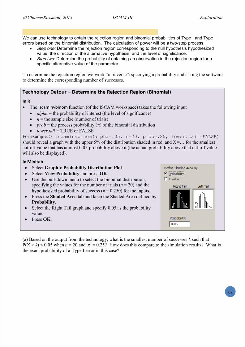
7/25/2019 Text: Investigating Statistical Concepts, Applications, and Methods
http://slidepdf.com/reader/full/text-investigating-statistical-concepts-applications-and-methods 63/428
Chance/Rossman, 2015 ISCAM III Exploration
S
9:'#"#8$8+6 /A?$':"+8'*I /A"7+ C8*';8"$ 9'G%: )"$74$"+8'*,We can use technology to obtain the rejection region and binomial probabilities of Type I and Type IIerrors based on the binomial distribution. The calculation of power will be a two-step process.
Step one: Determine the rejection region corresponding to the null hypothesis hypothesizedvalue, the direction of the alternative hypothesis, and the level of significance.
Step two : Determine the probability of obtaining an observation in the rejection region for aspecific alternative value of the parameter.
To determine the rejection region we work “in reverse”: specif ying a probability and asking the softwareto determine the corresponding number of successes.
!%7=*'$'>6 2%+'4: – 2%+%:;8*% +=% @%X%7+8'* @%>8'* OC8*';8"$P
M* @ The '()&*'.4='.1* function (of the ISCAM workspace) takes the following input
alpha = the probability of interest (the level of significance)
n = the sample size (number of trials) prob = the process probability ( ) of the binomial distribution lower.tail = TRUE or FALSE
For example: . ?9IB0?<HL?<C0&B486B!=-_Q <!#-Q 83CL!=#_Q 4C>;3=7B?4!RSEK'*should reveal a graph with the upper 5% of the distribution shaded in red, and X =… for the smallestcut-off value that has at most 0.05 probability above it (the actual probability above that cut-off valuewill also be displayed).
M* B8*8+"# Select Graph > Probability Distribution Plot Select View Probability and press OK . Use the pull-down menu to select the binomial distribution,
specifying the values for the number of trials ( n = 20) and thehypothesized probability of success ( = 0.250) for the inputs.
Press the Shaded Area tab and keep the Shaded Area defined byProbability .
Select the Right Tail graph and specify 0.05 as the probabilityvalue.
Press OK .
(a) Based on the output from the technology, what is the smallest number of successes k such thatP(X > k ) < 0.05 when n = 20 and = 0.25? How does this compare to the simulation results? What isthe exact probability of a Type I error in this case?
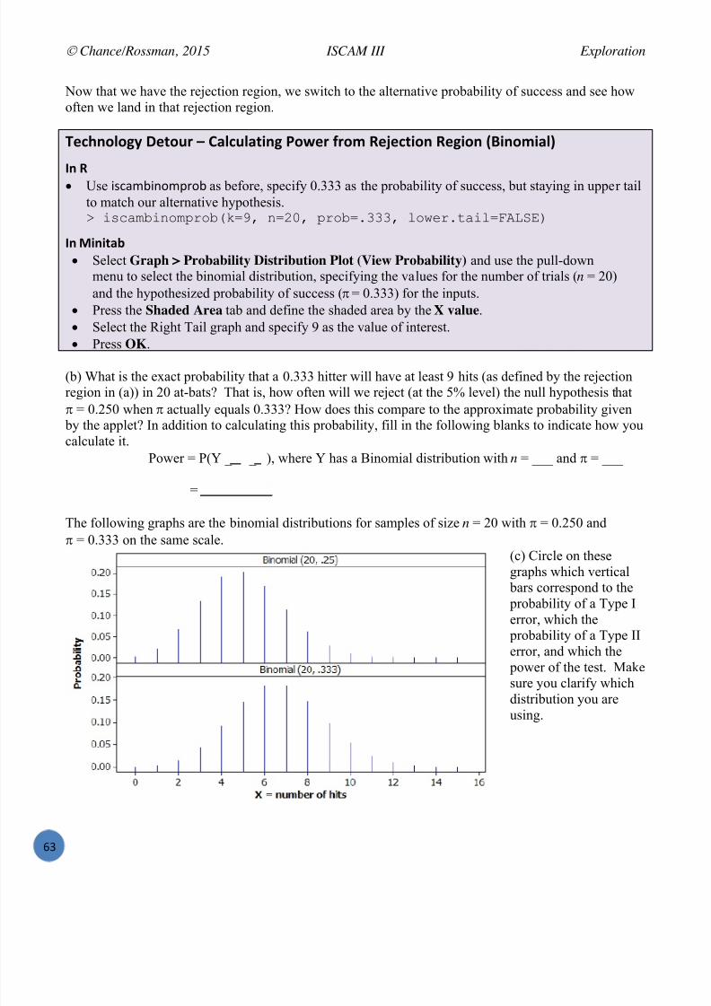
7/25/2019 Text: Investigating Statistical Concepts, Applications, and Methods
http://slidepdf.com/reader/full/text-investigating-statistical-concepts-applications-and-methods 64/428
Chance/Rossman, 2015 ISCAM III Exploration
S#
Now that we have the rejection region, we switch to the alternative probability of success and see howoften we land in that rejection region.
!%7=*'$'>6 2%+'4: – )"$74$"+8*> 9'G%: (:'; @%X%7+8'* @%>8'* OC8*';8"$P
M* @ Use '()&*='.1*851= as before, specify 0.333 as the probability of success, but staying in upper tail
to match our alternative hypothesis.. ?9IB0L?<C083CL&@!bQ <!#-Q 83CL!=(((Q 4C>;3=7B?4!RSEK'*
M* B8*8+"# Select Graph > Probability Distribution Plot (View Probability) and use the pull-down
menu to select the binomial distribution, specifying the values for the number of trials ( n = 20)and the hypothesized probability of success ( = 0.333) for the inputs.
Press the Shaded Area tab and define the shaded area by the X value . Select the Right Tail graph and specify 9 as the value of interest. Press OK .
(b) What is the exact probability that a 0.333 hitter will have at least 9 hits (as defined by the rejectionregion in (a)) in 20 at-bats? That is, how often will we reject (at the 5% level) the null hypothesis that
= 0.250 when actually equals 0.333? How does this compare to the approximate probability given by the applet? In addition to calculating this probability, fill in the following blanks to indicate how youcalculate it.
Power = P(Y _ _ ), where Y has a Binomial distribution with n = ___ and = ___
=
The following graphs are the binomial distributions for samples of size n = 20 with = 0.250 and = 0.333 on the same scale.(c) Circle on thesegraphs which vertical
bars correspond to the probability of a Type Ierror, which the
probability of a Type IIerror, and which the
power of the test. Makesure you clarify which
distribution you areusing.

7/25/2019 Text: Investigating Statistical Concepts, Applications, and Methods
http://slidepdf.com/reader/full/text-investigating-statistical-concepts-applications-and-methods 65/428
Chance/Rossman, 2015 ISCAM III Exploration
S
0";?$% 08E% 2%+%:;8*"+8'*(d) Suppose the player wants the power of correctly determining that he has become a 0.333 hitter to beat least 0.80. Use trial-and-error to determine the sample size necessary for him to achieve this.(Continue to assume the manager uses 0.05 as the level of significance.) [ Hint : Remember that you needto redo both steps in this process! Don’t forget to switch the value of …]
9:"7+87% 9:'#$%; HDY)(a) Repeat (a)-(d) of the Exploration using 0.01 as the level of significance.
(b) Did the sample size necessary to achieve power of at least 0.80 become larger or smaller with thissmaller significance level? Explain why this makes intuitive sense.

7/25/2019 Text: Investigating Statistical Concepts, Applications, and Methods
http://slidepdf.com/reader/full/text-investigating-statistical-concepts-applications-and-methods 66/428
Chance/Rossman, 2015 ISCAM III Investigation 1.7
SR
SECTION 2: NORMAL APPROXIMATIONS FOR SAMPLE PROPORTIONS
So far, all the studies you have examined have involved one categorical binary variable and therelevant statistic has been the number of successes, or equivalently the proportion of successes, where“success” is defined as the outcome you count (e.g., number of heart transplantation deaths, number ofhelper toys, number of hits) in a particular sample. You have used simulation from a coin-tossing typeprocess to approximate probabilities (p-value, error probabilities) and you calculated exact probabilitiesusing the binomial distribution.
Historically, when computers were less prevalent, these empirical and binomial probabilities were oftencumbersome to determine and statisticians instead applied a far more convenient approximationmethod to estimate the probabilities of interest. In this section, you will see how the normal probabilitymodel can be used as a third method to approximate the p-values, confidence intervals, and errorprobabilities from the previous section. See Chapter 2 for more information about the normaldistribution.
Investigation 1.7: Reese’s Pieces
Manufacturers often perform “quality checks ” to insure that their manufacturing process is operatingunder certain specifications. Suppose a manager at Hershey’s is concerned that his manufacturing
process is no longer producing the correct color proportions in Reese’s candies.
(a) Take a (presumably representative) sample of n = 25 Reese’s Pieces candies and record the numberof orange, yellow, and brown candies in your sample.
Orange: Yellow: Brown:
(b) Identify the observational units and variable for your sample.
Observational units:
Variable: Type:
(c) Define “success” to be an orange candy and “failure” to be a non -orange candy. Is it reasonable totreat these data as observations from a binomial process?
(d) Based on your data, do you think 0.50 is a plausible value for the probability Her shey’s process produces an orange candy? How are you deciding?
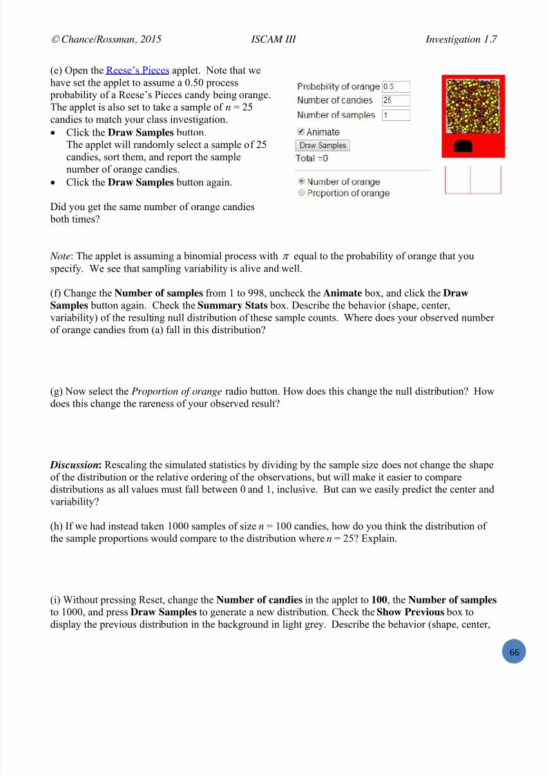
7/25/2019 Text: Investigating Statistical Concepts, Applications, and Methods
http://slidepdf.com/reader/full/text-investigating-statistical-concepts-applications-and-methods 67/428
Chance/Rossman, 2015 ISCAM III Investigation 1.7
S
(e) Open the Reese’s Pieces applet. Note that wehave set the applet to assume a 0.50 process
probability of a Reese’s Pieces candy being orange.The applet is also set to take a sample of n = 25candies to match your class investigation.
Click the Draw Samples button.The applet will randomly select a sample of 25candies, sort them, and report the samplenumber of orange candies.
Click the Draw Samples button again.
Did you get the same number of orange candies both times?
Note : The applet is assuming a binomial process with equal to the probability of orange that you
specify. We see that sampling variability is alive and well.
(f) Change the Number of samples from 1 to 998, uncheck the Animate box, and click the DrawSamples button again. Check the Summary Stats box. Describe the behavior (shape, center,variability) of the resulting null distribution of these sample counts. Where does your observed numberof orange candies from (a) fall in this distribution?
(g) Now select the Proportion of orange radio button. How does this change the null distribution? How
does this change the rareness of your observed result?
Discussion : Rescaling the simulated statistics by dividing by the sample size does not change the shapeof the distribution or the relative ordering of the observations, but will make it easier to comparedistributions as all values must fall between 0 and 1, inclusive. But can we easily predict the center andvariability?
(h) If we had instead taken 1000 samples of size n = 100 candies, how do you think the distribution of
the sample proportions would compare to the distribution where n = 25? Explain.
(i) Without pressing Reset, change the Number of candies in the applet to 100 , the Number of samplesto 1000, and press Draw Samples to generate a new distribution. Check the Show Previous box todisplay the previous distribution in the background in light grey. Describe the behavior (shape, center,

7/25/2019 Text: Investigating Statistical Concepts, Applications, and Methods
http://slidepdf.com/reader/full/text-investigating-statistical-concepts-applications-and-methods 68/428

7/25/2019 Text: Investigating Statistical Concepts, Applications, and Methods
http://slidepdf.com/reader/full/text-investigating-statistical-concepts-applications-and-methods 69/428
Chance/Rossman, 2015 ISCAM III Investigation 1.7
S
A very common and useful probability model is the normal distribution .9:'#"#8$8+6 2%+'4: – 3':;"$ @"*5'; J":8"#$%,Many quantitative variables have a distribution that can be reasonably modeled with a normal
probability curve . This is a continuous probability distribution (as opposed to the binomial, which is adiscrete distribution) that is specified by two quantities:
Mean, denoted by , which is the peak and point of symmetry Standard deviation, denoted by , which is the distance between the mean and the inflection points
In other words, the mean determines the center of the distribution, and the standard deviation controlshow variable (spread out) the distribution is. Standard deviation can be loosely interpreted as a typicaldistance of the observations from the mean.
This normal curve is given by the following function: N( ,
222
1
21
)( x
e x f < x <
Notes: The symbol is used here to refer tothe irrational number ≈ 3.14159… . Theconstant in front of the exponential termensures that the total area under any normalcurve equals one.
x Then the probability of an observation falling in any particular interval is determined by the area underthe normal curve in that interval. In principle, this area could be determined by integrating thefunction f ( x) above. But this particular function has no closed form anti-derivative, so we rely ontechnology to approximate these areas and therefore these normal probabilities.
For now, we will focus on using this mathematical model as an approximation to the distribution ofsample proportions. In this case, one can show (using some basic probability rules) that the theoreticalmean of the distribution of sample proportions will be equal to the process probability and the
theoretical standard deviation of this distribution equalsn
pSD )1(
)ˆ
(
.
(n) Calculate the theoretical mean and standard deviation of the sampling distribution of sample proportions for each of these three cases.
Theoretical mean of pˆ
Theoretical SD of pˆ
n = 25, = 0.5
n = 100, = 0.25
n = 100, = 0.80
How do the theoretical means and standard deviations compare to the simulated values (see the graphs before part (m)) and to each other?
f ( x)

7/25/2019 Text: Investigating Statistical Concepts, Applications, and Methods
http://slidepdf.com/reader/full/text-investigating-statistical-concepts-applications-and-methods 70/428
Chance/Rossman, 2015 ISCAM III Investigation 1.7
SV
(o) Now suppose we had taken samples of size n = 5 candies instead (from a process with success probability 0.80). Predict how the distribution of sample proportions will behave (shape, center,variability).
Shape: Mean: SD:
(p) Use the applet to check your predictions. Discuss your observations.
Discussion: It is very important to keep in mind that this normal probability model is not always a validapproximation for the distribution of sample proportions. Whether it is valid will be determined by acombination of the sample size n (larger samples result in more symmetric distributions) and the value
of (values closer to 0 or 1 result in less symmetric distributions). A common guideline is to assumesymmetry when n ! > 10 and n ! (1 ) > 10.
(q) Explain how these guidelines are consistent with your observations above.
This result about the long-run pattern of variation
in sample proportions is more formally called theCentral Limit Theorem (CLT) and is one of themost important results in Statistics. It states that ifthe sample size is large enough, then the samplingdistribution of the sample proportion p
ˆ
will bewell modeled by a normal distribution with meanE( p
ˆ
) equal to , the process probability, andstandard deviation
SD( pˆ
) equal ton
)1( .
The convention is to consider the sample size largeenough if n! 10 and n! (1 ) 10.
Binomial( n = 100, = 0.80) / 100
vs. Normal (mean = 0.80, SD = 0.040)
Discussion: Use of the normal probability model to approximate the sampling distribution of sample proportions is largely historical (back when they didn’t have computers, the binomial distributioncalculations were a bit of a pain but much easier with the normal distribution). But you will see in thenext few investigations that some calculations are still more convenient with the normal distribution.

7/25/2019 Text: Investigating Statistical Concepts, Applications, and Methods
http://slidepdf.com/reader/full/text-investigating-statistical-concepts-applications-and-methods 71/428
7/25/2019 Text: Investigating Statistical Concepts, Applications, and Methods
http://slidepdf.com/reader/full/text-investigating-statistical-concepts-applications-and-methods 72/428
Chance/Rossman, 2015 ISCAM III Investigation 1.8
TW
Investigation 1.8: Is ESP real?
Statistician Jessica Utts has conducted extensive analysis of studies that have investigated psychicfunctioning. (Combining results across multiple studies, often to increase power, is called meta-analysis. ) Utts (1995) cites research from Bern and Honorton (1994) that analyzed studies that used a
technique called ganzfeld.In a typical ganzfeld experiment, a “receiver” is placed in a room relaxing in a comfortable chair withhalved ping-pong balls over the eyes, having a red light shone on them. The receiver also wears a set ofheadphones through which [static] noise is played. The receiver is in this state of mild sensory deprivationfor half an hour. During this time, a “sender” observes a randomly chosen target and tries to mentallysend this information to the receiver … The recei ver is taken out of the ganzfeld state and given a set of
possible targets, from which they must decide which one most resembled the images they witnessed.Most commonly there are three decoys along with a copy of the target itself. [Wikipedia ]
(a) Suppose you want to test whether the subjects in these studies have ESP, with equal to the actual probability that they identify the correct image. State appropriate null and alternative hypotheses, insymbols and in words.
Ho:
Ha:
Utts cites Bern and Honorton as reporting that the studies showed 106 “hits” in 329 sessions. (Dr. Utts’report: www.ics.uci.edu/~jutts/air.pdf .)(b) Determine the sample proportion of hits, and denote it with an appropriate symbol.
(c) Although we know how to compute the exact binomial p-value for this test, in this investigation you
will use the normal probability model to approximate the binomial calculation. Assuming that thesubjects have no psychic ability, is this sample size large enough to allow using the Central LimitTheorem? Justify your answer with appropriate calculations.
(d) Describe what the Central Limit Theorem says about the distribution of sampling proportions in thiscontext, assuming the null hypothesis is true, and produce a well-labeled sketch to illustrate yourdescription.
(e) In your graph, shade the area under the curve corresponding to the sample proportion of “hits” b eing0.322 or higher.

7/25/2019 Text: Investigating Statistical Concepts, Applications, and Methods
http://slidepdf.com/reader/full/text-investigating-statistical-concepts-applications-and-methods 73/428
Chance/Rossman, 2015 ISCAM III Investigation 1.8
T
The area you have shaded represents the probability of a sample proportion exceeding 0.322, under theassumption that the subjects have no psychic ability (with n = 329 sessions).
(f) Based on your shading, provide a rough guess of this area as a percentage of the total area under thisnormal curve.
(g) How many standard deviations (SDs) above the mean is the value 0.322, the observed sample proportion of hits? [ Hint : First subtract the mean from 0.322, then divide the result by the SD.]
Definition: The standardized score of an observation determines the number of standard deviations between the observation and the mean of the distribution:
z = observation – mean = x
standard deviation This quantity is also referred to as the z-score. By converting to this z-score, we say we havestandardized the observation. This provides us another metric or ruler for how unusual an observation is.The sign of the z-score tells us whether the observation falls above or below the mean. If X follows anormal distribution with mean and standard deviation , then Z follows a normal distribution withmean 0 and standard deviation 1.
Because this z-score is larger than 2, we already know the probability to the right is rather small. Buthow can we determine this probability more precisely? Generally we would integrate the function overthe region of interval (0 .322, ∞). Because that is not possible wit h the normal probability function, wewill instead use technology, which implements numerical integration techniques to calculate this
area/probability.
!%7=*'$'>6 2%+'4: – )"$74$"+8*> 3':;"$ 9:'#"#8$8+8%,
M* @IThe '()&*.15*851= function takes the following inputs: xval = the x value of interest mean = the mean of the normal distribution sd = the standard deviation of the normal distribution direction = “above,” “below,” “outside” or “between” (using the quotes) label = a string of text (in quotes) to put on the horiziontal axis xval2 = an optional input for use with “outside” and “between” directions. digits = specifies how many significant digits to display, default is 4
For example (with or without input labels): ?9IB0<C3083CL&[HB4!=(##Q 0;B<!=#_Q 9A!=-#(acQA?3;I7?C<!5BLCH;5Q 4BL;4!59B084; 83C8C37?C<95*
M* B8*8+"# Choose Graph > Probability Distribution Plot (View Probability) Keep the Distribution pull-down menu set to Normal and specify the values for the mean and
standard deviation.
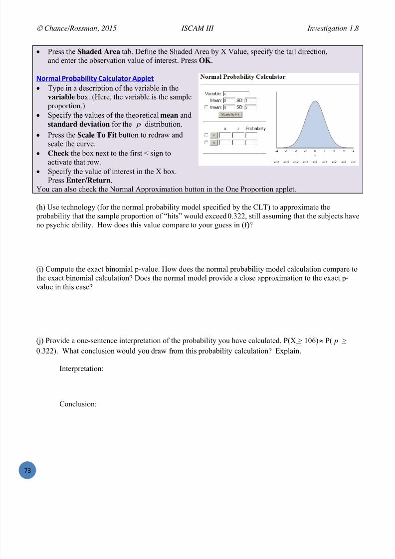
7/25/2019 Text: Investigating Statistical Concepts, Applications, and Methods
http://slidepdf.com/reader/full/text-investigating-statistical-concepts-applications-and-methods 74/428
Chance/Rossman, 2015 ISCAM III Investigation 1.8
T#
Press the Shaded Area tab. Define the Shaded Area by X Value, specify the tail direction,and enter the observation value of interest. Press OK .
3':;"$ 9:'#"#8$8+6 )"$74$"+': <??$%+ Type in a description of the variable in the
variable box. (Here, the variable is the sample proportion.)
Specify the values of the theoretical mean andstandard deviation for the p
ˆ
distribution. Press the Scale To Fit button to redraw and
scale the curve. Check the box next to the first < sign to
activate that row. Specify the value of interest in the X box.
Press Enter/Return . You can also check the Normal Approximation button in the One Proportion applet.
(h) Use technology (for the normal probability model specified by the CLT) to approximate the probability that the sample proportion of “hits” would exceed 0.322, still assuming that the subjects haveno psychic ability. How does this value compare to your guess in (f)?
(i) Compute the exact binomial p-value. How does the normal probability model calculation compare tothe exact binomial calculation? Does the normal model provide a close approximation to the exact p-value in this case?
(j) Provide a one-sentence interpretation of the probability you have calculated, P(X > 106) P( pˆ
>0.322). What conclusion would you draw from this probability calculation? Explain.
Interpretation:
Conclusion:
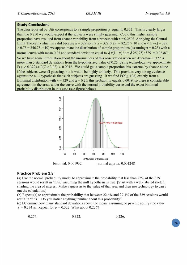
7/25/2019 Text: Investigating Statistical Concepts, Applications, and Methods
http://slidepdf.com/reader/full/text-investigating-statistical-concepts-applications-and-methods 75/428
Chance/Rossman, 2015 ISCAM III Investigation 1.8
T
0+456 )'*7$4,8'*,The data reported by Utts corresponds to a sample proportion p
ˆ equal to 0.322. This is clearly largerthan the 0.250 we would expect if the subjects were simply guessing. Could this higher sample
proportion have resulted from chance variability from a process with = 0.250? Applying the CentralLimit Theorem (which is valid because n = 329 so n ! = 329(0.25) = 82.25 > 10 and n ! (1 ) = 329! 0.75 = 246.75 > 10) we approximate the distribution of sample proportions (assuming = 0.25) with anormal curve with mean 0.25 and standard deviation equal to n/)1( = 329/)75(.25. = 0.02387.So we have some information about the unusualness of this observation when we determine 0.322 ismore than 3 standard deviations from the hypothesized value of 0.25. Using technology, we approximateP( p
ˆ
> 0.322) P(Z > 3.02) 0.0012. We could get a sample proportion this extreme by chance aloneif the subjects were all guessing, but it would be highly unlikely. This provides very strong evidenceagainst the null hypothesis that such subjects are guessing. If we find P(X > 106) exactly from aBinomial distribution with n = 329 and = 0.25, this probability equals 0.0019, so there is considerableagreement in the areas under the curve with the normal probability curve and the exact binomial
probability distribution in this case (see figure below).
binomial: 0.001932 normal approx: 0.001248
9:"7+87% 9:'#$%; HD[(a) Use the normal probability model to approximate the probability that less than 22% of the 329sessions would result in “hits,” assuming the null hypothesis is true. [Start with a well -labeled sketch,shading the area of interest. Make a guess as to the value of that area and then use technology to carryout the calculation.](b) Repeat (a) to approximate the probability that between 22.6% and 27.4% of the 329 sessions wouldresult in “hits.” Do you notice anything familiar about this probability?(c) Determine how many standard deviations above the mean (assuming no psychic ability) the value p
ˆ = 0.274 is. Repeat for pˆ = 0.322. What about 0.226?
0.274: 0.322: 0.226:

7/25/2019 Text: Investigating Statistical Concepts, Applications, and Methods
http://slidepdf.com/reader/full/text-investigating-statistical-concepts-applications-and-methods 76/428
Chance/Rossman, 2015 ISCAM III Investigation 1.9
TR
Investigation 1.9: Halloween Treat Choices
Obesity has become a widespread health concern, especially in children. Researchers believe that givingchildren easy access to food increases their likelihood of eating extra calories. Schwartz, Chen, andBrownell (2003) examined whether children would be willing to take a small toy instead of candy at
Halloween. They had seven homes in 5 different towns in Connecticut present children with a plate of 4toys (stretch pumpkin men, large glow-in-the-dark insects, Halloween theme stickers, and Halloweentheme pencils) and a plate of 4 different name brand candies (lollipops, fruit-flavored chewy candies,fruit- flavored crunchy wafers, and “sweet and tart” hard candies) to see whether children were morelikely to choose the candy or the toy. The houses alternated whether the toys were on the left or on theright. Data were recorded for 284 children between the ages of 3 and 14 (who did not ask for both typesof treats).
(a) Identify the observational units and variable of interest in this study. Is this variable quantitative orcategorical? If categorical, how many different outcomes are possible?
Observational units:Variable of interest:
Variable type: Possible outcomes:
(b) Define (in words) the parameter of interest in this study.
(c) State an appropriate null and alternative hypothesis involving this parameter (in symbols and inwords), for testing whether there is strong evidence of a preference for either the toys or the candy.
Ho:
Ha:
(d) In the sample of 284 children, 135 children chose the toy and 149 chose the candy. Calculate thevalue of a relevant statistic in this study.
(e) Is the sample size large enough for the conditions of the Central Limit Theorem to be met? Justifyyour answer with appropriate calculation(s).

7/25/2019 Text: Investigating Statistical Concepts, Applications, and Methods
http://slidepdf.com/reader/full/text-investigating-statistical-concepts-applications-and-methods 77/428
Chance/Rossman, 2015 ISCAM III Investigation 1.9
T
(f) According to the Central Limit Theorem, in considering the distribution of sample proportions
- What is the shape of the null distribution here?
- What is the mean of this distribution?
- What is the standard deviation of this distribution?
- Create a well-labeled sketch of the distribution under the null hypothesis; shade the region(s)of interest to represent the two-sided p-value for this test; and conjecture the magnitude ofthe p-value based on your sketch.
(g) Calculate the z-score for the observed sample proportion compared to the probability hypothesized by the null hypothesis.
(h) What does it mean for this z-score to be negative? What do you know about the z-score for the uppertail of the two-sided p-value? Explain.
Definition: The above calculation result comparing the observed statistic to the hypothesized parametervalue is more generally referred to as the test statistic . In the case of a single categorical variable with a
process probability of 0 (the value specified by the null hypothesis), the formula is:
n
p z
/)1(
ˆ
00
00

7/25/2019 Text: Investigating Statistical Concepts, Applications, and Methods
http://slidepdf.com/reader/full/text-investigating-statistical-concepts-applications-and-methods 78/428
Chance/Rossman, 2015 ISCAM III Investigation 1.9
TT
This test statistic is simply the application of the z-score from the previous investigation, and you willinterpret it as “how many standard deviations the observed proportion p
ˆ
lies from the hypothesized process proportion.” With the two -sided p-value, we are interested in how often we will obtain a p
ˆ
value as far from the hypothesized probability in either direction . Due to the symmetry of the normalcurve, this only involves doubling one of the tail probabilities.
(i) Based on the test statistic value you calculated, does the sample proportion appear to be extremeunder the null hypothesis?
(j) Use technology (e.g., Normal Probability Calculator applet) to determine the approximation to thetwo-sided p-value with the normal distribution. Is your p-value consistent with your sketch in (f)?
(k) Provide a one-sentence interpretation of this p-value.
(l) Based on this p-value, will you reject the null hypothesis at the 5% level of significance?
(m) Do you think the researchers are pleased by the lack of significance in this test? Explain, in thecontext of this study, why such a result might be good news for them.
(n) Does this mean the researchers can conclude that they have proven that children do not have a preference between candy and toys? Explain.
7/25/2019 Text: Investigating Statistical Concepts, Applications, and Methods
http://slidepdf.com/reader/full/text-investigating-statistical-concepts-applications-and-methods 79/428
Chance/Rossman, 2015 ISCAM III Investigation 1.9
T
0+456 )'*7$4,8'*,If we define to be the probability that, when presented with a choice of candy or a toy while trick-
or-treating, a child chooses the toy, and if we assume the null hypothesis (H 0: = 0.5) is true, the abovecalculations tell us that we would observe at most 135 children choosing candy (at least 149 choosingtoy) or at most 135 of the 284 children choosing the toy in about 40% of samples. Thus, this is not asurprising outcome when = 0 .5. We fail to reject the null hypothesis and conclude that it’s plausiblethat children are equally split in preferring the toy or the candy.
We do have some cautions with this study as it was conducted in only a few households inConnecticut, a “convenience sample, ” so we cannot claim that these results are representative ofchildren in other neighborhoods. We also don’t know if the children found the toys “novel” and whethertheir preference for toys could decrease as the novelty wears off (or if “better” candy choices wereoffered). Furthermore, when the children approached the door they were asked their age and gender,and for a description of their Halloween costume. The researchers caution that that this may have cuedthe children that their behavior was being observed (even though their responses were recorded byanother research member who was out of sight) or that they should behave a certain way. Still, theseresearchers were optimistic that alternatives could be presented to children, even at Halloween, to lessentheir exposure to large amounts of candy.
M;?:'F8*> +=% "??:'A8;"+8'*(o) Use technology to determine the exact binomial p-value. How does it compare to the normalapproximation in this case?
Even though our sample size is reasonably large (for the Central Limit Theorem), there is still some“discreteness” in the exact binomial distribution that makes the normal approximation (which, of course,is continuous) less accurate than we would like. With the normal distribution, P(X < k ) = P(X < k )
because P(X = k ) = 0 for any particular (integer) value k . However, P(X = k ) > 0 with the binomialdistribution. It is the failure to include the “mass” at k that can lead the normal approximation to be poor.How can we correct for this? We can apply a continuity correction by using the normal distribution tocalculate P(X < k + 0.5) as an approximation for P(X ≤ k ) and P(X > k 0.5) as an approximation forP(X > k ).
(p) In order to calculate P(X < 135), what probability does the continuity correction tell us to calculate?
(q) In order to calculate P(X > 149), what probability does the continuity correction tell us to calculate?[ Hint : Remember what the continuity correction is trying to accomplish.]

7/25/2019 Text: Investigating Statistical Concepts, Applications, and Methods
http://slidepdf.com/reader/full/text-investigating-statistical-concepts-applications-and-methods 80/428
Chance/Rossman, 2015 ISCAM III Investigation 1.9
TV
(r) Use technology (e.g., Normal Probability Calculator applet) to re-approximate the p-value using thenormal probability distribution with the continuity correction. How does this new approximationcompare to the earlier one (without the continuity correction) and to the exact binomial p-value?
Many software programs allow you to do this continuity correction for a one-sample z-test (e.g., using p
ˆ
= (X 0.5)/n as the input) or may do so by default. However, when n is large, you may not seemuch difference in the values.
!%7=*'$'>6 2%+'4: – 3':;"$ <??:'A8;"+8'* +' C8*';8"$
!=%':6\C",%5 M*(%:%*7% <??$%+ Enter the sample size and either the count
or the proportion of successes, press
Calculate to display sample data. Check the box for Test of significance Specify the hypothesized value Use the button to specify the direction of
the alternative Press the Calculate button. Check the cont corr. box to apply the
continuity correction to the test statisticand p-value.
M* @IThe '()&*='.1*.15*F>7 .7 851=7 ;'5,)%'1.G function gives a visual of this continuity correction. It
takes the following inputs: k = the observation of interest n = the sample size prob = the process probability ( ) direction = “below,” “above,” or “two.sided”
(s) Use technology to verify your calculations.

7/25/2019 Text: Investigating Statistical Concepts, Applications, and Methods
http://slidepdf.com/reader/full/text-investigating-statistical-concepts-applications-and-methods 81/428
Chance/Rossman, 2015 ISCAM III Investigation 1.9
U
9:"7+87% 9:'#$%; HD]< A student wanted to assess whether her dog Muffin tends to chase her blue ball and her red ball equallyoften when they are rolled at the same time. The student rolled both balls a total of 96 times, each timekeeping track of which ball Muffin chased. The student found that Muffin chased the blue ball 52 timesand the red ball 44 times. Let’s treat the blue ball as “success.”
(a) State the appropriate null and alternative hypotheses in symbols. (Be sure to describe what thesymbol represents in this context.) (b) Report and interpret the values of the z-test statistic and normal-based p-value.(c) Summarize yo ur conclusion about the student’ s question concerning her dog Muffin.(d) Explain the reasoning process behind your conclusion. (e) Suppose you want to redo this study using a sample size of 200 tosses. You plan to use asignificance level of = 0.05, and you are concerned about the power of your test when = 0.60.Explain how you would determine this power (the two steps) and interpret what “power” implies in thiscontext.(f) How would your answers to the previous questions change if we had used the red ball as success?
9:"7+87% 9:'#$%; HD]CSuppose that you want to re-conduct the kissing study in a large city with a sample of 100 kissingcouples. You want to test the null hypothesis H 0: = 0.667 against a one-sided alternative H a: < 0.667using a significance level of = 0.05, and you are concerned about the power of your test when = 0.5.Consider the following graph:
(a) Which region(s) represents the probability of making a Type I error?I II III IV
(b) Which region(s) represents the probability of making a Type II error?I II III IV
(c) Which region(s) represents the power of the test?I II III IV

7/25/2019 Text: Investigating Statistical Concepts, Applications, and Methods
http://slidepdf.com/reader/full/text-investigating-statistical-concepts-applications-and-methods 82/428
Chance/Rossman, 2015 ISCAM III Investigation 1.9
UW
04;;":6 '( '*% ?:'?':+8'* ! \+%,+Let represent the (constant) probability of success for the process assumed by the null hypothesis.
To test H 0: = 0 We can calculate a p-value based on the normal distribution with mean equal to 0 and standarddeviation equal to n/)1( 00
Test Statistic:n
p z
/)1(
ˆ
00
00 which follows a N(0,1) distribution
p-value: if H a: > 0: p-value = P( Z > z 0)if H a: < 0: p-value = P( Z < z0)if H a: ≠ 0: p-value = 2P( Z > | z0|)
Validity: This procedure is considered valid as long as the sample size is large relative to thehypothesized probability ( n ! 0 > 10 and n ! (1 0) > 10), and you have a representative samplefrom the process of interest.
Technology Theory-Based Inference applet
Specify the hypothesized value, use the button to specify the direction of the alternative (< > for notequal), enter the sample size and either the count or the proportion of successes. Press the Calculate
button. R, ISCAM Workspace: '()&*1.,8518K%,(%F!"#$%&$' 7( 7)*+!,)$#-.$' X7/0,$%(/,-&$ _`35,&%,5`7
`-,((`7 15 `%<1/(';,;`7 )1.9/-,4,-G You can enter either the number of successes or the proportion of successes ( p
ˆ
) for the “observed”value. If you don’t specify a hypothesized value and alternative, be sure to label the confidence level
Minitab: Choose Stat > Basic Statistics > 1 Proportion (now using the Method pull-down menu toselect Normal approximation under Options ). It is good practice to also produce the graph of the normal probability distribution ( Graph >Probability Distribution Plot ) showing the p-value shaded. Use two-sided alternatives to determinea confidence interval.

7/25/2019 Text: Investigating Statistical Concepts, Applications, and Methods
http://slidepdf.com/reader/full/text-investigating-statistical-concepts-applications-and-methods 83/428

7/25/2019 Text: Investigating Statistical Concepts, Applications, and Methods
http://slidepdf.com/reader/full/text-investigating-statistical-concepts-applications-and-methods 84/428
Chance/Rossman, 2015 ISCAM III Investigation 1.10
U#
(e) Use the distance in (d) and the observed sample proportion of pˆ
= 0.645 to determine an interval of plausible values for , the probability that a kissing couple leans to the right.
An approximate 95% confidence interval for the process probability based on the normal distributionwould be p
ˆ 2 n p p /)ˆ
1(ˆ . That is, this interval extends two standard deviations on each side of the
sample proportion. We know that for the Normal distribution roughly 95% of observations (here sample proportions) fall within 2 SDs of the mean (here the unknown population proportion), so this methodwill “capture ” the process probability for roughly 95% of samples.
However, we should admit that the multiplier of 2 is a bit of a simplification. So how do we find a more precise value of the multiplier to use, including for values other than 95%? We will use technology to dothis. Keep in mind that the z-value corresponding to probability C in the middle of the distribution, alsocorresponds to having probability (1 C )/2 in each tail.
!%7=*'$'>6 2%+'4: – L8*58*> 9%:7%*+8$%, (:'; +=% 0+"*5":5 3':;"$ 28,+:8#4+8'*
3':;"$ 9:'#"#8$8+6 )"$74$"+': "??$%+ You can leave the mean set to zero and the standard deviation to 1 and the variable is “z -scores.” Check the box next to the first < sign and specify the probability value to correspond to the lower
tail probability of interest, (1 C )/2. Press Enter/Return and it will display the negative z-value.
M* @IThe '()&*'.4.15* function takes the following inputs: Probability of interest Mean = the mean of the normal distribution (default = 0)
Standard deviation = the standard deviation of the normal distribution (default = 1) Direction = whether the probability of interest was in the lower tail (“below”) or the upper tail
(“above”), in both tails (“outside”), or in the middle of the distribution (“between”) For example: ?9IB0?<H<C30&83CL!=b_Q A?3;I7?C< ! 5L;7>;;<5*
M* B8*8+"# Choose Graph > Probability Distribution Plot (View Probability) . Keep the Distribution pull-down menu set to Normal (with mean 0 and SD 1). Press the Shaded Area tab. Define the Shaded Area by the Probability value, specify the tail, and
enter the corresponding probability value (e.g., 0.025 in lower tail or 0.05 in Both Tails or 0.025 and0.025 in Middle). Press OK twice.
(f) Use technology to more precisely determine the number of standard deviations that capture themiddle 95% of the normal distribution with mean = 0 and standard deviation = 1. [ Hint : In other words,how many standard deviations do you need to go on each side of zero to capture the middle 95% of thedistribution?]

7/25/2019 Text: Investigating Statistical Concepts, Applications, and Methods
http://slidepdf.com/reader/full/text-investigating-statistical-concepts-applications-and-methods 85/428
Chance/Rossman, 2015 ISCAM III Investigation 1.10
U
Definition: The (100 ! C )% critical value , z*, is the z-score valuesuch that P( z* ≤ Z ≤ z*) = C where C is any specified probabilityvalue, and Z represents a normal distribution with mean 0 and SD 1.
Note: We use the symbol z* to distinguish this value, found based on
the confidence level, from z0, the observed z-score for the data.
(g) Find the critical value for a 90% confidence interval. Is it larger orsmaller than with 95% confidence? Why does this make sense?
Putting these together, we have a one-sample z-interval (aka Wald interval) for a process probability:One sample z -confidence interval (or “Wald interval”) for : When we have at least 10 successesand at least 10 failures in the sample, an approximate confidence interval for is given by:
pˆ
+ z* n p p )
ˆ
1(ˆ
(h) Based on this formula, what is midpoint of the interval? What determines the width of the interval?
Midpoint: Width:
(i) How does increasing the confidence level affect the width of the interval?
How does increasing the sample size affect the width of the interval?
(j) Use this procedure to calculate (by hand) and interpret a 90% confidence interval, based on thenormal probability model, for the probability a kissing couple leans to the right.
(k) How do the midpoint and width of the 90% confidence interval compare to those of the 95%confidence interval? Also verify your claims in (h) about the midpoint and width based on this 90%confidence interval.
Definition: The half-width of the interval is also referred to as the margin-of-error . So the above interval formula is of the common form: statistic margin-of-error, where margin-of-error = critical value ! standard error of statistic .

7/25/2019 Text: Investigating Statistical Concepts, Applications, and Methods
http://slidepdf.com/reader/full/text-investigating-statistical-concepts-applications-and-methods 86/428
Chance/Rossman, 2015 ISCAM III Investigation 1.10
UR
Although 95% is the most common confidence level, a few other confidence levels and theircorresponding critical values are shown in the table below.Confidence level 90% 95% 99% 99.9%Critical value z * 1.645 1.960 2.576 3.291
!%7=*'$'>6 2%+'4: – -*% ?:'?':+8'* ! \7'*(85%*7% 8*+%:F"$,E\8*+%:F"$ G8+= @ Use '()&*1.,8518K%,(%F1=(,54,;7 .7 +681%+,(K',;7 &-%,5.&%'4,_`35,&%,5`7 ̀ -,((7` 15
`%<1/(';,;`7 )1.9/-,4,-G You can enter either the number of successes or the proportion of successes ( p
ˆ
) for the“observed” value. If you don’t specify a hypothesized value and alternative, be sure to label theconfidence levelFor example: ?9IB0C<;83C8d7;97&CL9;3H;A!a-Q <!,#]Q IC<G=4;H;4!b_*
E\8*+%:F"$ G8+= B8*8+"#
Choose Stat > Basic Statistics > 1 Proportion . Specify the column with the data or enter the Summarized data: count of success (an integer)and sample size.
Press Options and make sure the Alternative is set to “not equal”; use the Method pull-downmenu to select Normal approximation. Press OK twice.
E\8*+%:F"$ G8+= !=%':6\C",%5 M*(%:%*7% "??$%+ Keep the pull-down menu set to One proportion . Specify the sample size n and either the count or
the sample proportion. Or check the Paste Data box and paste in the individual outcomes (checkthe Includes header box if you are also copyingover the variable name).
Press Calculate .
Check the box for Confidence interval Change the confidence level from 95 to 90 % Press the Calculate CI button
(l) Now use technology to find and report the 90% and 95% confidence intervals for the probability thata kissing couple leans to the right. Did the widths and midpoints behave as you conjectured above?
(m) How do these intervals compare to the Exact Binomial Confidence Intervals reported by R?b- 8;3I;<7 IC<G?A;<I; ?<7;3HB4: -=_^a(^cb -=c,^^]^-b_ 8;3I;<7 IC<G?A;<I; ?<7;3HB4: -=__]##b^ -=c#aba(#
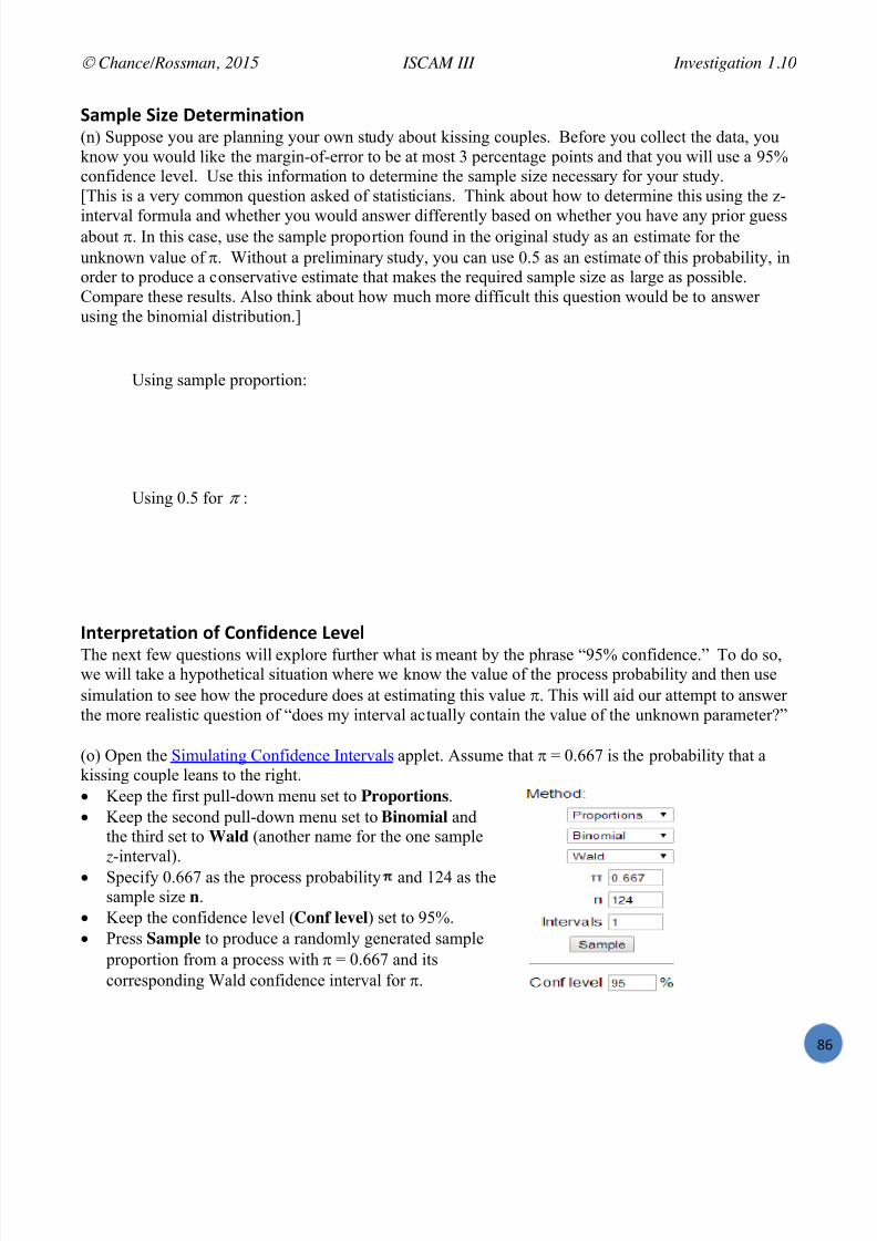
7/25/2019 Text: Investigating Statistical Concepts, Applications, and Methods
http://slidepdf.com/reader/full/text-investigating-statistical-concepts-applications-and-methods 87/428

7/25/2019 Text: Investigating Statistical Concepts, Applications, and Methods
http://slidepdf.com/reader/full/text-investigating-statistical-concepts-applications-and-methods 88/428
Chance/Rossman, 2015 ISCAM III Investigation 1.10
UT
Did this interval capture the value of (0.667)? [ Hint : The interval will be green if 0.667 is inside theinterval and red if not.]
(p) Click on the interval itself, and the midpoint of the interval will display (at the bottom), as well as the
endpoints. Record these values.
Midpoint: Lower endpoint: Upper endpoint:
(q) Press Sample again. Did you get the same value of pˆ
?
New interval:
Did you get the same interval?
Does this surprise you?
Did the value of change?
Did the new interval capture the value of ?
(r) Now change the number of intervals ( Intervals ) to 198 (for a total of 200 intervals) and pressSample . What percentage of these 200 random intervals successfully capture 0.667 (see the RunningTotal )?
Is this close to what you expected?
(s) Also press Sort , and comment on what the intervals that fail to successfully capture 0.667 have incommon.
(t) Change the number of intervals to 200 and press Sample four more times. Examine the RunningTotal for these 1000 intervals. Is this percentage (of intervals that successfully contain the valueunderlying parameter value 0.667) close to what you expect?
Definition: The confidence level of an interval procedure is supposed to indicate the long-run percentage of intervals that capture the actual parameter value, if repeated random samples were takenfrom the process. As such the confidence level presents a measure of the reliability of the method. Aconfidence interval procedure is considered valid when the achieved long-run coverage rate matches (orcomes close to) the stated (also called nominal) confidence level.
7/25/2019 Text: Investigating Statistical Concepts, Applications, and Methods
http://slidepdf.com/reader/full/text-investigating-statistical-concepts-applications-and-methods 89/428
Chance/Rossman, 2015 ISCAM III Investigation 1.10
U
(u) Based on your simulation results above, does this one-sample z-interval appear to be a valid 95%confidence interval procedure in this case? Explain.
(v) Predict what will be different about 90% confidence intervals compared to the 95% confidenceintervals. ( Hint : Try to list two differences.)
(w) Press the Sort button and then change the confidence level to 90% and press Recalculate . What isthe primary change in the properties of these intervals?
In particular, does the coverage rate appear to now differ from 95%? Explain.
(x) Predict what will be different about these 90% confidence intervals if we double the sample size.Also predict what (if anything) will be different about the running percentage of intervals that succeed incapturing the parameter value.
(y) Change the sample size n to 248 (twice as large as before) and press Sample five times to generate1000 intervals. What is the primary change in the properties of these intervals?
Does the (long-run) confidence level appear to now differ from 90%?
Discussion: In real life, you only take one sample, and you cannot know whether it’s going to produce agreen or a red interval! So what does “95% confidence” mean? These simulations reveal that if we takerepeated random samples from a process with probability and calculate a (100 ! C )% confidenceinterval each time, then in the long-run roughly (100 ! C )% of the resulting intervals succeed incapturing inside the interval. So when we gather the actual sample data and calculate a single interval,
we say tha t we are “ (100!
C )% confident” that this interval succeeds in capturing the actual value of the process probability ; and the basis for our confidence is knowing that in the long run the procedurewould generate a successful interval in (100 ! C )% of all possible samples. We also noted that samplesize will affect the width or “precision” of the interval but not the confidence level.
(z) Suppose that you take 1000 random samples from a process and generate a 95% confidence intervalfor with each sample. If you randomly select one of these intervals, what is the probability that youwill select an interval that captures ?

7/25/2019 Text: Investigating Statistical Concepts, Applications, and Methods
http://slidepdf.com/reader/full/text-investigating-statistical-concepts-applications-and-methods 90/428

7/25/2019 Text: Investigating Statistical Concepts, Applications, and Methods
http://slidepdf.com/reader/full/text-investigating-statistical-concepts-applications-and-methods 91/428
Chance/Rossman, 2015 ISCAM III Investigation 1.11
V
Investigation 1.11: Heart Transplant Mortality (cont.)
Recall Investigation 1.3, where you learned that 8 of the 10 most recent heart transplantation operationsat St. George’s Hospital resulted in a death.
(a) Use the one sample z-interval method to find a 95% confidence interval for the probability of a hearttransplantation death at St. George’s hos pital. Does anything bother you about doing this?
To consider whether the above procedure is valid, we can again pretend we know the process probability, generate many random samples and calculate confidence intervals from them, and see what percentage of these confidence intervals capture the actual value.
(b) In the Simulating Confidence Intervals applet, suppose the actual process probability of death is 0.15and you plan to take a sample of 10 operations and apply the z-interval procedure. Use the applet toexplore the reliability (empirical coverage rate) of this method for these data. That is, generate 1000intervals (200 at a time) with = 0.15 and n = 10 and see how many of these intervals succeed incapturing the actual value of the population parameter (0.15). Is this coverage rate close to 95%?
(c) Explain why you should not expect the coverage rate to be close to 95% in this case.
Because the z-interval procedure has the sample size conditions of the Central Limit Theorem, there arescenarios where we should not use this z-procedure to determine the confidence interval. One option isto return to calculating a confidence interval based on the Binomial distribution. However, this is a fairlycomplicated method (as opposed to: “go two standard deviations on each side”) and often producesintervals that are wider than they really need to be (the actual coverage rate is higher than the nominalconfidence level). An alternative method that has been receiving much attention of late is often calledthe Plus Four procedure (in contrast to the Wald procedure we’ve been using): The idea is to pretendyou have 2 more successes and 2 more failures than you really did (the “Wilson adjustment”) .
Definition: Plus Four 95% confidence interval for : Determine the number of successes (X) and sample size ( n) in the study
Increase the number of successes by two and the sample size by four. Make this value themidpoint of the interval: p~ = (X + 2)/( n + 4) Use the z-interval procedure as above for the augmented sample size of ( n + 4):
4)~1(~
96.1~n
p p p
Note : For confidence levels other than 95%, researchers have recommended using the Adjusted Wald method: p~ = (X + 0.5 z*2)/(n + z*2) and n
~ = n + z*2 so the interval becomes p~ z* n p p ~/)~1(~ .

7/25/2019 Text: Investigating Statistical Concepts, Applications, and Methods
http://slidepdf.com/reader/full/text-investigating-statistical-concepts-applications-and-methods 92/428
Chance/Rossman, 2015 ISCAM III Investigation 1.11
VW
(d) Investigate the reliability of the Plus Four procedure:In the Simulating Confidence Intervals applet Use the second pull-down menu to change from
Wald to Plus Four . Generate 1000 confidence intervals from a process
with = 0.15 and n = 10.
Is this coverage rate close to 95%? Is this an improvement over the (Wald) z-interval?
(e) Use the second pull-down menu to toggle between the Wald and Plus Four intervals. [ Hint: You canSort the intervals first.] What do you notice about how the midpoints of the intervals compare? (Alsothink how p~ and p
ˆ
differ.) Why is that useful in this scenario?
Researchers have determined that this method does have much better coverage properties, even for verysmall sample sizes, and tends to produce intervals that are narrower than the binomial intervals. Somestatisticians have gone so far as to argue that this is the only procedure that should be used for aconfidence interval for a process probability.
(f) Use the Plus Four procedure to determine and interpret a 95% confidence interval for the probabilityof a death during a hear t transplant operation at St. George’s hospital. [ Hints : You can do the calculation
either by hand, first finding p~ and z*, or with the Theory-Based Inference applet or Minitab or R bytelling the technology there were 4 more operations consisting of two more deaths than in the actualsample.]
(g) Repeat for the larger study at St. George’s th at revealed 71 deaths out of 361 operations. How do the95% Wald and Plus Four intervals compare in this case?
Wald interval: Plus Four interval:
Comparison:

7/25/2019 Text: Investigating Statistical Concepts, Applications, and Methods
http://slidepdf.com/reader/full/text-investigating-statistical-concepts-applications-and-methods 93/428
Chance/Rossman, 2015 ISCAM III Investigation 1.11
V
Discussion As you can tell, there are several ways to obtain a confidence interval for a process probability. When the sample size is large, they will yield very similar results for the endpoints and thecoverage rate. When the sample size is small, the “Adjusted Wald” method is preferred (or theBinomial but it tends to be more conservative and doesn’t have the estimate margin-of-error simplicity). Below we compare the 95% confidence intervals for the 8 of 10 and 71 of 361 studies for
these methods plus a fourth, the “Wilson interval” which is a more direct inversion of the one sample proportion z-test.
Exact Binomial (aka Clopper-Pearson)Finds the values of so the P(X < k ) > C )/2 and P(X > k ) >(1 C )/2 where k is observed number of successesTends to be “conservative” (longer than necessary)
n = 10
(.4439, .9748)
n = 361
(.1569, .2415)Minitab or
R using '()&*='.1*%,(%
Wald interval (aka normal approximation aka asymptotic)
Finds the values of so that P( z <n p p
p
/)ˆ
1(ˆ
ˆ
< z) = C
Formula: pˆ
+ z* n p p )ˆ
1(ˆ
Tends to show poor coverage properties if small n or extreme
(.5521, 1.048) (.1557, .2377)
TBI applet or Minitabor R ( '()&*1.,8518K%,(% )
Plus Four (aka Agresti-Coull, special case of Adjusted Wald)(95%) Add two successes and two failures to sample resultsFormula: p~ + z* n p p ~/)~1(~ where p~ = (X + 0.5 z2)/(n + z2) and n
~ = n + z2 Very good coverage properties
(.4776, .9509) (.1590, .2410)
TBI applet or Minitab or R aftermaking adjustment to sample data
Wilson interval (aka Score interval)
Finds the values of so that P( z <n
p
/)1(
ˆ
< z) = C
Formula:n z
n
zn
p p z z
n p
2
2
22
14
)ˆ
1(ˆ
21ˆ
Very good coverage properties. Very similar to Adjusted Waldfor 95% confidence.
(.4902, .9433) (.1590, .2408)R 8518/%,(% w/o continuity corr.
(.4422, .9646) (.1577, .2423)R 8518/%,(% w/ continuity corr.
Many statisticians now view the Plus Four or Adjusted Wald method as the best in terms of coveragerate and width (Binomial intervals, because of the discreteness, are often wider than they “need” to be ),as well as simplicity.
Whatever procedure is used to determine the confidence interval, you interpret a (valid) interval thesame way – as the interval of plausible values for the parameter. For example, we are 95% confidentthat the underlying probability of death within 30 days of a heart transplant operation at St. George’sHospital is between 0.16 and 0. 24; where by “95% confident ,” we mean that if we were to use this

7/25/2019 Text: Investigating Statistical Concepts, Applications, and Methods
http://slidepdf.com/reader/full/text-investigating-statistical-concepts-applications-and-methods 94/428
Chance/Rossman, 2015 ISCAM III Investigation 1.11
V#
procedure to construct intervals from thousands of representative samples, roughly 95% of thoseintervals will succeed in capturing the actual (but unknown) value of the parameter of interest.
^%%? 8* B8*5I The main things you should focus on in your study of confidence intervals are:
What parameter is the interval estimating (in context)? What are the effects of sample size, confidence level, and p
ˆ
on the width and midpoint interval? What do we mean by “confidence”? What are the effects (if any!) of sample size, confidence level, and p
ˆ
on the coverage rate of themethod?
Why might one confidence interval method be preferred over another?
Also note how to use R, Minitab, or the Theory-Based Inference applet to perform these calculations.You should NOT use the Simulating Confidence Intervals applet to construct a confidence interval for a
particular sample of data.
9:"7+87% 9:'#$%; HDHH Return to your exploration using the Simulating Confidence Intervals applet. Assume that = 0.667 isthe probability that a kissing couple leans to the right.(a) From the third pull-down menu select the Wilson (aka Score) interval method. Evaluate the
performance of this interval method, clearly explaining your steps.
(b) Starting withˆ
(1 ) /
p z
n
, use the quadratic formula to solve for and verify the formula for
the Wilson interval.(c) Show that with 95% confidence the Wilson formula simplifies to approximately the Plus Fourmethod.

7/25/2019 Text: Investigating Statistical Concepts, Applications, and Methods
http://slidepdf.com/reader/full/text-investigating-statistical-concepts-applications-and-methods 95/428

7/25/2019 Text: Investigating Statistical Concepts, Applications, and Methods
http://slidepdf.com/reader/full/text-investigating-statistical-concepts-applications-and-methods 96/428
Chance/Rossman, 2015 ISCAM III Investigation 1.12
VR
The authorship of literary works is often a topic for debate. Were some of the works attributed toShakespeare actually written by Bacon or Marlowe? Which of the anonymously published FederalistPapers were written by Hamilton, which by Madison, which by Jay? Who were the authors of thewr itings contained in the Bible? The field of “literary computing” examines ways of numericallyanalyzing authors’ works, looking at variables such as sentence length and rates of occurrence of
specific words.
The above passage is of course Abraham Linco ln’s Gettysburg Address, given November 19, 1863 onthe battlefield near Gettysburg, PA. In characterizing this passage, we would ideally examine everyword. However, often it is much more convenient and even more efficient to only examine a subset ofwords.
Definition: The population is the entire collection of observational units that we are interested in. Asample is the subset of the population for which we collect data.In this case you will examine data for just 10 of the words. We are considering this passage to be a
population of 268 words, and the 10 words you selected are therefore a sample from this population.
In most statistical studies, we do not have access to the entire population and can consider only data fora sample from that population. Our ultimate goal is to make conclusions about the larger population,
based on only the sample data.
Up until now, we have generally been assuming we have a representative sample from an infinite on-going process (e.g., dog identification of cancer sample, hospital transplant operations, candymanufacturing). We made some assumptions, like the process is not changing over time and that thereis no tendency to select some types of outcomes more than others (e.g., getting the first 5 candies fromthe manufacturing process rather than throughout the day). In fact, a binomial process assumes you haverepeat observations from the exact same process but with randomness in the actual outcome that occurs
(sometimes the dog makes the correct identification, some time she does not).In this case, instead of sampling from an on-going process we are sampling from a finite population (the268 words). In fact, we actually have access to the entire population. But what if we didn’t? We stillneed some way of convincing people that are sample is likely to be representative of the population. Todo that, we will explore for a minute, using this population to see how samples behave where “randomchance” arises from which observational units are selected to be in the sample, rather than from “randomchoices” made by th e observational units.
(b) Consider the sample you selected in (a). Suppose I wanted to focus on the lengths of the words in thesample (if the sample is truly representative, it shouldn’t matter what variable I end up recording).
Record the ten lengths that you found.
1 2 3 4 5 6 7 8 9 10Length
(c) Identify the observational units and variable for this sample.
Obs units: Variable: Type:

7/25/2019 Text: Investigating Statistical Concepts, Applications, and Methods
http://slidepdf.com/reader/full/text-investigating-statistical-concepts-applications-and-methods 97/428

7/25/2019 Text: Investigating Statistical Concepts, Applications, and Methods
http://slidepdf.com/reader/full/text-investigating-statistical-concepts-applications-and-methods 98/428

7/25/2019 Text: Investigating Statistical Concepts, Applications, and Methods
http://slidepdf.com/reader/full/text-investigating-statistical-concepts-applications-and-methods 99/428

7/25/2019 Text: Investigating Statistical Concepts, Applications, and Methods
http://slidepdf.com/reader/full/text-investigating-statistical-concepts-applications-and-methods 100/428

7/25/2019 Text: Investigating Statistical Concepts, Applications, and Methods
http://slidepdf.com/reader/full/text-investigating-statistical-concepts-applications-and-methods 101/428

7/25/2019 Text: Investigating Statistical Concepts, Applications, and Methods
http://slidepdf.com/reader/full/text-investigating-statistical-concepts-applications-and-methods 102/428

7/25/2019 Text: Investigating Statistical Concepts, Applications, and Methods
http://slidepdf.com/reader/full/text-investigating-statistical-concepts-applications-and-methods 103/428
Chance/Rossman, 2015 ISCAM III Investigation 1.13
W
Investigation 1.13: Literary Digest
Literary Digest was a well-respected political magazine founded in 1890. Using sampling, theycorrectly predicted the presidential outcomes from 1916 – 1932. In 1936, they conducted the mostextensive (to that date) public opinion poll in history. They mailed out questionnaires to over 10 million
people (about one-third of U.S. households) whose names and addresses they obtained from telephone books and vehicle registration lists. More than 2.4 million responded, with 57% indicating that theywould vote for Republican Alf Landon in the upcoming presidential election.
(a) Identify the population of interest, the sample, and the sampling frame in this study. Also define the parameter and statistic, in words and symbols, and indicate any values that you know.
Population of interest
Sample
Sampling frameParameter
Statistic
(b) Have you ever heard of Alf Landon? He lost. By a landslide. Incumbent Democrat FranklinRoosevelt won the election, carrying 63% of the popular vo te to Landon’s 37%. Give two explanationswhy the Literary Digest prediction was so much in error. In particular, talk about the direction of the
bias – why was this sampling method vulnerable to producing an overestimate of the parameter?
Discussion: There are two main issues here. One, the sampling frame did not include all members ofthe population of interest and failed to include those that were poorer (and at that time likely to beDemocrat). Second, the voluntary response nature of the poll implies the surveyors were more likely tohear from those unhappy with the status quo or with more time on their hands to complete such surveys(e.g., retired folks), and even those more willing to pay for a stamp. All of these probably point to anoverrepresentation of Republicans. Bad sampling frames and voluntary response bias are perhaps themost common sources of sampling error. By the way, a fledgling pollster of the time, George Gallup,actually bet that he would predict the percentages more accurately. Not only did he correctly predict the
Digest result with only 3,000 respondents, he also correctly predicted a Roosevelt victory!

7/25/2019 Text: Investigating Statistical Concepts, Applications, and Methods
http://slidepdf.com/reader/full/text-investigating-statistical-concepts-applications-and-methods 104/428
Chance/Rossman, 2015 ISCAM III Investigation 1.13
WX#
9:"7+87% 9:'#$%; HDHT< In the mid-1980s, Shere Hite undertook a survey of women's attitudes toward relationships, love, andsex by distributing 100,000 questionnaires in women's groups. Of the 4500 who returned thequestionnaire, 96% said that they gave more emotional support than they received from their husbandsor boyfriends. An ABC News/Washington Post poll surveyed a random sample of 767 women, finding
that 44% claimed to give more emotional support than they received.
(a) Which of the following is t he “parameter” of interest in these studies? Those who said they gave more emotional support All American women The 4500 women who responded The proportion who said they received less emotional support Other
(b) Which poll ’s results do you think are more representative of the population of all American women?Explain.
9:"7+87% 9:'#$%; HDHTCAn article published in the June 6, 2006 issue of the journal Pediatrics describes the results of a surveyon the topic of college students intentionally injuring themselves. Researchers invited 8300undergraduate and graduate students at Cornell University and Princeton University to participate in thesurvey. A total of 2875 students responded, with 17% of them saying that they have purposefullyinjured themselves. Suppose we are interested in the proportion of self-injuries in the population of allcollege students.(a) Identify the observational units and variable in this study. Also classify the variable as categorical(also binary?) or quantitative.
(b) Identify the parameter and statistic. Also indicate appropriate symbols.(c) Do you think it likely that this sample is representative of the population of all college students in theworld? What about all college students in the U.S.? Explain.(d) Describe a population you might be willing to generalize the results to.(e) For which of the following variables would you suspect this sample would be representative of the
population of all U.S. college students? Justify your answer.
Favorite TV show Height Parental education Eye color
9:"7+87% 9:'#$%; HDHT)
(a) Does your class constitute a random sample of students from your school? Explain why or why not.(b) Suggest a variable for which your class should not be considered a representative sample of allstudents at your school. Explain why not.(c) Suggest a variable for which it might be reasonable to consider your class to be representative of allstudents at your school. Justify your choice.

7/25/2019 Text: Investigating Statistical Concepts, Applications, and Methods
http://slidepdf.com/reader/full/text-investigating-statistical-concepts-applications-and-methods 105/428
Chance/Rossman, 2015 ISCAM III Investigation 1.14
W
Investigation 1.14: Sampling Words (cont.)
In this section, we have transitioned from sampling from an infinite process to sampling from a finitepopulation. We discussed randomly selecting the sample from a list of the entire population as a wayto convince us that the sample is likely to be representative of the larger population and therefore weare willing to generalize results from our sample to the larger population. The second benefit ofconsciously introducing this randomness into the study design is that the resulting sample statistics willfollow a predictable pattern as suggested in Investigation 1.12, allowing us to measure the strength ofevidence against claims about the population parameter and the margin-of-error in our estimates of theparameter. We will again consider simulation-based p-values, exact p-values, and a mathematicalmodel for estimating the p-value and confidence interval.
0+"+8,+87"$ M*(%:%*7%To calculate p-values and confidence intervals, we would like to examine all possible samples of size n from the population and calculate the statistic for each sample to understand the amount of sample-to-sample variation by chance alone. However, this is not usually feasible. Even for samples of size 5from a population of 268 words, there are C(268, 5) or more than 11 billion possible samples! Instead,we will use technology to take a large number of random samples to estimate the behavior of thedistribution of the sample statistics in this rare case where we have access to the entire population.
(a) Open the Sampling Words applet. You will notice that the applet displays ahistogram of word lengths for the entire population. Use the Variable pull-downmenu to select HasE to focus on the variable of whether or not the word containsat least one e.The applet displays the distribution of “ e-words” and “non -e-words.” Is this variable quantitative orcategorical?
(b) What is the value of the parameter (proportion of e-words) for this population? What symbol can weuse to represent this value?
(c) Check the Show Sampling Options box. Specify 1000 as the Number of Samples and 5 as theSample Size . Press the Draw Samples button. Describe the resulting distribution of sample
proportions. Be sure to explain what the mean and standard deviation represent here.
(d) Does the random sampling performed by this applet appear to be an unbiased sampling method toestimate the population proportion? Explain how you are deciding.
7/25/2019 Text: Investigating Statistical Concepts, Applications, and Methods
http://slidepdf.com/reader/full/text-investigating-statistical-concepts-applications-and-methods 106/428
Chance/Rossman, 2015 ISCAM III Investigation 1.14
WXR
/((%7+ '( 0";?$% 08E%(e) Change the sample size to 20 press Draw Samples. Discuss how this change has impacted the bias ofthe sampling method and/or the precision. [ Hint : Examine the reported mean and standard deviation.] Isthis what you expected?
/((%7+ '( 9'?4$"+8'* 08E%(f) Now select the ! 4 radio button on the left to make four copies of the population Your population nowconsists of the four copies of the Gettysburg Address, a total of 1072 words. Now what is the value ofthe population proportion of successes ( e-words)?
(g) Generate 1000 random samples of n = 20 words from this new population, and observe thedistribution of 1000 sample proportions. Compare how the shape, mean, and standard deviation compareto that from (e).
Mean: Standard deviation: Shape:
Comparison:
Is this what you expected?
(h) Repeat (g) using forty addresses as the population, now containing 10,720 words.
Mean: Standard deviation: Shape:
Discussion: You should notice that the population size did not make much of a difference in thedistribution of sample proportions! This will be true as long as the population size is large compared tothe sample size. In this case, the small sample we are removing from the population is not changing the
population much (so the probability the next word contains the letter e is pretty much the same as the probability the first word selected would) and we can consider the observations to be approximatelyindependent (the subsequent probability of success to be approximately constant) . This means it’s justlike we are sampling from an infinite process…
(i) In Investigation 1.7, we stated that the mean of a distribution of sample proportions from a processequals and the standard deviation equals n)1( . Calculate these theoretical values and comparethem to the applet results for n = 20.
Theoretical Mean: Theoretical Standard deviation:
Comparison to applet results:

7/25/2019 Text: Investigating Statistical Concepts, Applications, and Methods
http://slidepdf.com/reader/full/text-investigating-statistical-concepts-applications-and-methods 107/428
Chance/Rossman, 2015 ISCAM III Investigation 1.14
W
(j) Does the formula for the standard deviation presented in (i) consider the size of the population? Isthis consistent with what you observed in (g) and (h)?
(k) When n = 20 does the distribution of sample proportions appear to be well-modeled by a normaldistribution? (Check the Overlay Normal Distribution box to help you decide.)
In fact, the distribution of sample proportions when taking simple random samples from a populationshould remind you very much of the distribution of sample proportions when sampling from a process,such as the Reese’s Pieces investigation. In fact, the same “Central Limit Theorem” result also holds inthis case of sampling from a population, with one additional caveat about the relative sizes of the sampleand population, as summarized below:
Key Result: The Central Limit Theorem for a sample proportion states that when drawing randomsamples from a large but finite population with a large enough sample size, then the samplingdistribution of the sample proportion p
ˆ
will be well modeled by a normal distribution with mean equal
to , the population proportion of successes, and standard deviation equal to n pSD /)1()ˆ
( .We consider the sample size large enough if n! > 10 and n! (1 ) > 10.We consider the population size ( N ) large if it is more than 20 times the size of the sample. If the population size is not large, we would use a different standard deviation formula that incorporatesa “finite population correction factor.” Probability sampling methods other than simple randomsampling would also require calculating a different standard deviation. You can learn more appropriatetechniques in a course on sampling design and methods.
This result means that the normal-based procedures for making inferences about an underlying process also apply for making inferences from sample data to a larger population , provided that the sample isselected randomly from the (large) population.
Discussion: Once again you see the fundamental principle of sampling variability . Fortunately, thisvariability follows a predictable pattern in the long run. You should see that the average of the sample
proportions is approximately equal to the population proportion, = 0.466, as we would expect becausethe simple random sampling method is unbiased. [The mean of your empirical sampling distributionmay not be exactly equal to as you only took 1000 samples instead of all possible samples of size 5 or20, but we are no longer consistently overestimating the population parameter as we would with thenonrandom samples.] The second key advantage of randomly sampling is that this predictable patternwill allow us to estimate how far the sample statistic is likely to fall from the population parameter andwhen we might have a surprising value for the sample statistic. Of course our level of surprise willdepend on the sample size because you also saw that the amount of sampling variability in the sample
proportion decreases when we increase the sample size. Sample proportions that are based on largersamples will tend to fall even closer to the population proportion and thus there is less variabilityamong the sample proportions. So first, select randomly to avoid bias, and then if we can increase the

7/25/2019 Text: Investigating Statistical Concepts, Applications, and Methods
http://slidepdf.com/reader/full/text-investigating-statistical-concepts-applications-and-methods 108/428
Chance/Rossman, 2015 ISCAM III Investigation 1.14
WXT
sample size, this will improve the precision of the sample results. Once we know the precision of thesample results in repeated samples, then we can decide whether any one particular sample result can beconsidered statistically significant or unlikely to happen by chance – the random sampling process – alone. A small p-value does not guarantee that the sample result did not happen just by chance, but itdoes allow you to measure how unlikely such a result is.
In the next investigation you will consider a method for computing an “exact” p -value, taking the population size into account. However, in many situations we don’t know the size of the population, just that it is large, and instead we will proceed directly to the normal-based method, as long as thetechnical conditions are met.
9:"7+87% 9:'#$%; HDHU (a) Which of the following are advantages of studies with a larger sample size? ( Check all that apply )
Better represent the population (reduce sampling bias) To more precisely estimate the parameter To decrease sampling variability
To make simulation results more precise Other?
(b) In conducting a simulation analysis, why might we take a larger number of samples? ( Check all thatapply )
Better represent the population (reduce sampling bias) To more precisely estimate the parameter To decrease sampling variability To make simulation results more precise Other?

7/25/2019 Text: Investigating Statistical Concepts, Applications, and Methods
http://slidepdf.com/reader/full/text-investigating-statistical-concepts-applications-and-methods 109/428

7/25/2019 Text: Investigating Statistical Concepts, Applications, and Methods
http://slidepdf.com/reader/full/text-investigating-statistical-concepts-applications-and-methods 110/428
Chance/Rossman, 2015 ISCAM III Investigation 1.15
WXV
(d) Identify some precautions taken by these students to avoid nonsampling errors.
In this study the sample results were that 22 of the 30 first-years planned to vote for John Kerry, whereas8 planned to vote for George Bush.(e) Construct a bar graph to display the results for this sample and write a one-sentence summary ofwhat the graph reveals.
(f) Define the parameter of interest in this study. What symbol would we use to represent this value?
As in Investigation 1.13, we are considering these data to be a random sample from a finite population(not a simple random sample but we will ignore that distincti on for now). However, we don’t haveaccess to the population. We can still predict how the outcomes from many different random sampleswill behave by using a probability model. That is, we want to know the random behavior of X, thenumber of Kerry voters in the sample.
(g) Explain why we cannot treat X as a binomial random variable.
When sampling from a finite population, the appropriate probability model is a hypergeometricdistribution (see the Probability Detour). This gives us
P(X = k ) =),(
),(),(n N C
k n M N C k M C
where N is the population size, M is the number of successes in the population, and n is the sample size.
(h) Suppose 352 first-year students at this school (essentially 50% of the population) plan to vote forKerry. Use the hypergeometric distribution to calculate the probability of observing 22 or more studentsin a random sample of 30 students favoring Kerry. Would the sample result obtained by these students
be surprising?

7/25/2019 Text: Investigating Statistical Concepts, Applications, and Methods
http://slidepdf.com/reader/full/text-investigating-statistical-concepts-applications-and-methods 111/428
Chance/Rossman, 2015 ISCAM III Investigation 1.15
W
9:'#"#8$8+6 2%+'4: – .6?%:>%';%+:87 @"*5'; J":8"#$%, To be a hypergeometric random variable , a random process must have the following properties:
Observations are drawn without replacement from a population of N objects.There are two distinct types of objects in the population, M successes and N – M failures.
The main distinction between a hypergeometric random variable and a binomial random variable is thetrials are no longer independent. The probability of drawing a success for the first object is M / N . But ifwe do draw a success, then the probability of success for the second object is ( M – 1)/( N – 1). If wereplaced the item, then we would be back to a binomial process.
So to calculate hypergeometric probabilities, we need to consider another probability rule.When outcomes are equally likely, then the probability of an event equals the number of ways for the event to happen divided by the number of possible outcomes.
For example, there are 268 words in the Gettysburg Address, 123 contain the letter e (about 46%) and145 do not. Using counting rules, there are C(268, 5) = 11,096,761,368 different samples of 5 words thatwe could select from the Gettysburg Address. But if we want to select one e-word and four non- e-words, there are C(123, 1) ! C(145, 4) = 2,172,945,060 such samples. Thus we find P(one e-word),
P(X = 1) = 2,172,945,060 / 11,096,761,368 0.1958.
In general, the probability of obtaining k successes from a population with M successes and N – M
failures is P(X = k ) =),(
),(),(n N C
k n M N C k M C where C( a , b) =
)!(!!
baba
b
a
The expected value of the hypergeometric random variable is E(X) = ( M / N )! n and the standarddeviation is 1)()()()( N - / N - n /N ! N - M ! M/N n ! . (Compare these to binomial with = M / N .)
C8*';8"$ <??:'A8;"+8'* +' .6?%:>%';%+:87 28,+:8#4+8'*IIf we instead used the binomial distribution toapproximate this probability, we would find
P(X = 1) = C(5, 1)(125/268)(143/268) 4 0.1890.
These probability calculations work out to be verysimilar! This happens when the finite population weare sampling from is large compared to our samplesize (e.g., N > 20 ! n).
This means we can continue to use the binomialdistribution to determine such probabilities and theexpected number of successes 5(0.466) 2.33 withSD(X) 1.115 successes.
And when the sample size is large relative to the probability of success, we can approximate the binomial with the normal distribution.

7/25/2019 Text: Investigating Statistical Concepts, Applications, and Methods
http://slidepdf.com/reader/full/text-investigating-statistical-concepts-applications-and-methods 112/428

7/25/2019 Text: Investigating Statistical Concepts, Applications, and Methods
http://slidepdf.com/reader/full/text-investigating-statistical-concepts-applications-and-methods 113/428
Chance/Rossman, 2015 ISCAM III Investigation 1.15
W
Discussion: The hypergeometric distribution is able to tell us if we listed all possible samples of 30students from this population, how many would be at least as extreme as the observed sample. In manysampling situations, our population size is large enough that the binomial distribution gives a veryreasonable approximation to the exact p-value. For this reason, the binomial p-value is much morecommonly used than the hypergeometric p-value.
0+456 )'*7$4,8'*,Only about 0.68% of random samples from a population where the two candidates were equally
preferred would have 22 or more successes (Kerry voters) by random chance alone. This gives us verystrong evidence that more than 50% of this population was in favor of Kerry. In fact, we also found that2/3 is a plausible (believable) value for the population proportion in favor of Kerry. We applied thehypergeometric distribution because we had a small population rather than an infinite process, but the
population was large enough that we could have applied the binomial distribution instead.
9:"7+87% 9:'#$%; HDHV Reconsider the voter pattern study. Is 60% a plausible value for the percentage of students at thisuniversity who were in favor of Kerry? Justify your answer.

7/25/2019 Text: Investigating Statistical Concepts, Applications, and Methods
http://slidepdf.com/reader/full/text-investigating-statistical-concepts-applications-and-methods 114/428
7/25/2019 Text: Investigating Statistical Concepts, Applications, and Methods
http://slidepdf.com/reader/full/text-investigating-statistical-concepts-applications-and-methods 115/428
Chance/Rossman, 2015 ISCAM III Investigation 1.16
W
Investigation 1.16: Teen Hearing Loss
Shargorodsky, Curhan, Curhan, and Eavey (2010) examined hearing loss data for 1771 participants fromthe National Health and Nutrition Examination Survey (NHANES, 2005-6), aged 12-19 years.(“NHANES provides nationally representative cross -sectional data on the health status of the civilian,
non-institutionalized
U.S. population.” ) In this sample, 333 were found to have at least some level ofhearing loss. News of this study spread quickly, many blaming the prevalence of hearing loss on thehigher use of ear buds by teens. At MSNBC.com (8/17/2010), Carla Johnson summarized the study withthe headline “1 in 5 U.S. teens has hearing loss, study says.” We wil l first decide whether we considerthis an appropriate headline.
(a) Define the population and parameter of interest in this study (in symbols and in words).
Population:
Parameter:
(b) State the null and alternative hypotheses for deciding whether these data provide convincingevidence against this headline (in symbols and in words).
Discussion: A consequence of the expansion of the Central Limit Theorem we made in the previousinvestigation is that we can use all the same normal-based z-procedures when we have a large enoughsample size and have taken a random sample from a large population.
(c) Under the null hypothesis, is the normal model appropriate for the distribution of sample proportions based on this sample size and on this population size? Justify your answers numerically.
(d) Use technology to carry out a z-test of the hypotheses you specified in (b). Report the test statisticand p-value, and confirm how you would calculate the test statistic by hand.

7/25/2019 Text: Investigating Statistical Concepts, Applications, and Methods
http://slidepdf.com/reader/full/text-investigating-statistical-concepts-applications-and-methods 116/428
7/25/2019 Text: Investigating Statistical Concepts, Applications, and Methods
http://slidepdf.com/reader/full/text-investigating-statistical-concepts-applications-and-methods 117/428
Chance/Rossman, 2015 ISCAM III Investigation 1.16
W
04;;":6 '( -*% 9:'?':+8'* ! \9:'7%54:%, (': 9:'?':+8'* '( K":>% 9'?4$"+8'*Let the (unknown) population proportion of successes and given that you have a representative samplefrom the population of interest.
Test of H 0: = 0 Test statistic : z0 = ( p
ˆ
0)/ n/)1( 00 p-value :
If Ha: > 0, the p-value is P(Z > z0).If Ha: < 0, the p-value is P(Z < z0).If Ha: ≠ 0, the p-value is 2P(Z > | z0|)
C% confidence interval for Wald Interval: p
ˆ
n p p z /)ˆ
1(ˆ
* where z* is the 100 ! (1 C )/2 th percentile of the standardnormal distribution.Technical conditions: n > 10 and n(1 ) > 10 (which means there are at least 10 successes and10 failures in the sample) and population size > 20 n.
Adjusted Wald Interval: p~ + z* n p p ~/)~1(~ where p~ = (X + 0.5 z*2)/(n + z*2) and n~
= n + z*2 (For 95% confidence, add two successes and two failures, aka Plus Four Method.)Technical conditions: population size > 20 n
In Theory-Based Inference applet: One Proportion Specify the sample size and either the sample count or the sample proportion
- Remember to adjust these values if performing the Adjusted Wald interval Check the Test of Significance box and/or the Confidence Interval box
- Specify the value of 0, use the < button to change the direction of the alternative- Specify the confidence level
In R: '()&*1.,8518K%,(%F1=(,54,;7 .7 +681%+,('K,;7 &-%,5.&%'4,7 )1.9/-,4,-G Specify the number of successes or p
ˆ
, n, 0, alternative, and confidence level (in that order)- Remember to adjust inputs if performing the Adjusted Wald interval
For the alternative, choose “two.sided” or “less” or “greater” (with the quotes) If no alternative is specified, be sure to label the confidence level (conf.level)
In Minitab: Stat > Basic Statistics > One Proportion Specify a column of data or the Summarized data (sample count and sample size)
Check the box if you want to perform a hypothesis test Under Options use the Method pull-down menu to select Normal approximation , set theConfidence level, and/or specify the direction of the alternative
- Changing the method here gives you the calculations using the Central Limit Theorem - Use a two-sided alternative to get a two-sided confidence interval - Remember to consider the Adjusted Wald (Plus Four) interval procedure
May give you a warning message if the sample size condition is not met (but ignore if Adjusted Wald)
pˆ
pˆ

7/25/2019 Text: Investigating Statistical Concepts, Applications, and Methods
http://slidepdf.com/reader/full/text-investigating-statistical-concepts-applications-and-methods 118/428

7/25/2019 Text: Investigating Statistical Concepts, Applications, and Methods
http://slidepdf.com/reader/full/text-investigating-statistical-concepts-applications-and-methods 119/428
Chance/Rossman, 2015 ISCAM III Investigation 1.18
W
Discussion: Keep in mind the difference between statistical significance and practical significance . With large sample sizes, sample proportions will vary little from sample to sample, and so even smalldifferences (that may seem minor to most of us) will be statistically significant. Saying that a sampleresult is unlikely to happen by chance (and therefore is statistically significant) is not the same as sayingthe result is important or even noteworthy (practically significant), depending on the context involved.
Investigation 1.18: Female Senators
Suppose that an alien lands on Earth, notices that there are two different sexes of the human species, andsets out to estimate the proportion of humans who are female. Fortunately, the alien had a goodstatistics course on its home planet, so it knows to take a sample of human beings and produce aconfidence interval. Suppose that the alien happened upon the members of the 2015 U.S. Senate as itssample of human beings, so it finds 20 women and 80 men in its sample.
(a) Use this sample information to form a 95% confidence interval for the actual proportion of allhumans who are female.
(b) Is this confidence interval a reasonable estimate of the actual proportion of all humans who arefemale?
(c) Explain why the confidence interval procedure fails to produce an accurate estimate of the population parameter in this situation.
(d) It clearly does not make sense to use the confidence interval in (a) to estimate the proportion ofwomen on Earth or even the U.S., but does the interval make sense for estimating the proportion ofwomen in the 2015 U.S. Senate? Explain your answer.
Discussion: First, statistical tests and confidence intervals do not compensate for the problems of a biased
sampling procedure. If the sample is collected from the population in a biased manner, the ensuingconfidence interval will be a biased, and potentially misleading, estimate of the population parameterof interest.

7/25/2019 Text: Investigating Statistical Concepts, Applications, and Methods
http://slidepdf.com/reader/full/text-investigating-statistical-concepts-applications-and-methods 120/428
Chance/Rossman, 2015 ISCAM III Example 1.1
WWV
A second important point to remember is that confidence intervals and significance tests use samplestatistics to estimate population or process parameters. When the data at hand constitute the entire
population of interest, then constructing a confidence interval from these data is meaningless. In thiscase, you know precisely that the proportion of women in the population of the 2015 U.S. Senators is0.20 (exactly! no margin-of-error!), so it is senseless to construct a confidence interval from these
data.
Example 1.1: Predicting Elections from Faces?Try these questions yourself before you use the solutions following to check your answers.
Do voters make judgments about a political candidate based on his/her facial appearance? Can youcorrectly predict the outcome of an election, more often than not, simply by choosing the candidatewhose face is judged to be more competent-looking? Researchers investigated this question in a study
published in Science (Todorov, Mandisodka, Goren, and Hall, 2005). Participants were shown picturesof two candidates and asked who has the more competent looking face. Researchers then predicted thewinner to be the candidate whose face was judged to look more competent by most of the participants.
For the 32 U.S. Senate races in 2004, this method predicted the winner correctly in 23 of them.(a) In what proportion of the races did the “competent face” method predict the winner correctly?
(b) Describe (in words) the null model to be investigated with this study.
(c) Describe how you could (in principle) use a coin to produce a simulation analysis of whether thesedata provide strong evidence that the “competent face” method would correctly predict the electionwinner more than half the time. Include enough detail that someone else could implement the fullanalysis and draw a reasonable conclusion.
(d) Use the One Proportion Inference applet to conduct a simulation (using 1000 samples) addressingthe question of whether the researchers’ results provide strong evidence in support of the researchers’conjecture that the “competent face” method would correctly predict the election winner more than halfthe time. Be sure to report (and indicate on the dotplot), the p-value from the simulation.
(e) Write a paragraph, as if to the researchers, describing what your simulation analysis reveals aboutwhether the data provide strong evidence in support of their conjecture.

7/25/2019 Text: Investigating Statistical Concepts, Applications, and Methods
http://slidepdf.com/reader/full/text-investigating-statistical-concepts-applications-and-methods 121/428
Chance/Rossman, 2015 ISCAM III Example 1.1
W
(f) These researchers also predicted the outcomes of 279 races for the U.S. House of Representatives in2004. The “competent face” method correctly predicte d the winner in 189 of those races. Do you predictthis p-value will be larger or smaller than in (d)? Explain your reasoning.
<*"$6,8,(a) This method predicted the winner correctly in 23/32 ≈ 0.719 of the races.(b) The null model is that the “competent face” method is not useful for predicting election winners, soit would work in only 50% of all races in the long run.(c) You would flip a fair coin 32 times, once for each of the election races. Keep track of the number ofheads, representing races for which the method correctly predicted the winner. Repeat simulating 32
flips a large number of times. Determine the proportion of samples in which 23 or more coin tossesresulted in heads. If this proportion is very small, conclude that the competent face method really does
predict the winner correctly more than half the time.
(d) Here is a graph of the null distribution of 1000 simulated results under the null model:
Based on these 1000 samples, the approximate p-value is 12/1000 = 0.012. (Your approximate p-value will probably be different but close to this. The exact Binomial p-value equals 0.01.)
(e) This analysis reveals that it would be quite surprising to correctly predict 23 or more of 32 electionraces if the “competent face” method were no better than flipping a coin. More specifically, such anextreme result would only occur about 1% of the time by random chance. So, the data provide fairlystrong evidence in support of the researchers’ conjecture that the “competent face” method works morethan half the time.
(f) The observed proportion of successes is now 189/279 ≈ 0.677. This is not quite as extreme (far from0.5) as the first study, but the sample size is much larger. For this reason, you probably expect the p-value to be even smaller. (Indeed, the p-value now dips below 0.001.)
7/25/2019 Text: Investigating Statistical Concepts, Applications, and Methods
http://slidepdf.com/reader/full/text-investigating-statistical-concepts-applications-and-methods 122/428
Chance/Rossman, 2015 ISCAM III Example 1.2
W!W
Example 1.2: Cola DiscriminationTry these questions yourself before you use the solutions following to check your answers.
A teacher doubted whether his students could distinguish between the tastes of different brands of cola,so he presented each of his 21 students with three cups. Two cups contained one brand of cola, and the
third cup contained a different brand. Which cup contained which brand was randomly determined foreach student. Each student was asked to identify which cup contained the cola that was different fromthe other two. It turned out that 12 of the students successfully identified the “odd” cola.
(a) Does this result provide strong evidence that these students do better than guessing in discriminatingamong the colas? Address this question with an appropriate test of significance, including a statementof the hypotheses and a p-value calculation or estimation. Be sure to clarify which procedure you used todetermine the p-value and why. Summarize your conclusion, and explain the reasoning process bywhich it follows.
(b) Calculate a 95% confidence interval based on these sample data. Clearly define the parameter thatthis interval estimates, and interpret the interval.
(c) Would this teacher be convinced that his students do better than guessing if he uses the 0.05significance level?

7/25/2019 Text: Investigating Statistical Concepts, Applications, and Methods
http://slidepdf.com/reader/full/text-investigating-statistical-concepts-applications-and-methods 123/428

7/25/2019 Text: Investigating Statistical Concepts, Applications, and Methods
http://slidepdf.com/reader/full/text-investigating-statistical-concepts-applications-and-methods 124/428
Chance/Rossman, 2015 ISCAM III Example 1.2
W!#
<*"$6,8,(a) We can define to be the probability that these students correctly identify the odd soda. (In otherwords, if this group of students were to repeat this process under identical conditions indefinitely, represents the long-term fraction that they would identify correctly.) The null hypothesis asserts that thestudents are just guessing, which means that their success probability is one-third (H 0: = 1/3). Thealternative hypothesis is that students do better than guessing, which means that their success probabilityis greater than one-third (Ha: > 1/3).
Under the null hypothesis that the students are just guessing among the three cups, X has a binomialdistribution with parameters n = 21 and = 1/3. The normal distribution would probably not be validhere as we do not satisfy the conditions: n ! = 21(1/3) = 7 < 10. We could simulate observations fromthis Binomial process using the One Proportion Inference applet, and see how often we observe 12 ormore correct identifications just by chance:
Or we could calculate the exact Binomial probability, either with this applet or with
. ?9IB0L?<C083CL&@!,#Q <!#,Q 83CL!=((((Q4C>;3=7B?4!RSEK'*f3CLBL?4?71 ,# B<A BLCH; ! -=-#,,cc,(
or using '()&*='.1*%,(% :. ?9IB0L?<C07;97&CL9;3H;A!,#Q <!#,Q618!=((((Q B47;3<B7?H;!5D3;B7;35*
'[BI7 e?<C0?B4 U;97%B7B: CL9;3H;A 92II;99;9 ! ,#Q 9B084; 9?d; ! #,Q 9B084; 83C8C37?C< ! -=_c,] g244 618C76;9?9 : 8? ! -=((((S47;3<B7?H; 618C76;9?9: 8? . -=((((8)HB42;: -=-#,,cc

7/25/2019 Text: Investigating Statistical Concepts, Applications, and Methods
http://slidepdf.com/reader/full/text-investigating-statistical-concepts-applications-and-methods 125/428
Chance/Rossman, 2015 ISCAM III Example 1.2
W
Notice the normal approximation does not provide a great estimate of this p-value. ?9IB0C<;83C8d7;97&CL9;3H;A!,#Q <!#,Q 618!=((((QB47;3<B7?H;!5D3;B7;35*h<; f3C8C37?C< d 7;97
%B7B: CL9;3H;A 92II;99;9 ! ,#Q 9B084; 9?d;! #,Q 9B084; 83C8C37?C< ! -=_c,]
g244 618C76;9?9 : 8? ! -=((((S47;3<B7?H; 618C76;9?9: 8? . -=((((d)97B7?97?I: #=(,8)HB42;: -=-,-(,
But the normal approximation does improve with the continuitycorrection. ?9IB0L?<C0<C30&@!,#Q <!#,Q 83CL!=((((QA?3;I7?C<!5BLCH;5*
L?<C0?B4: -=-#,,a<C30B4 B883C[: -=-,-(,<C30B4 B883C[ >?76 IC<7?<2?71: -=-,a^-
This p- value reveals that if the students were just guessing, there’s only about a 2% probability of “bychance” getting 12 or more correct identifications among 21 trials. I n other words, if we repeated thisstudy over and over, and if students were just guessing each time, then a result this favorable wouldoccur in only about 2% of the studies. Because this probability is quite small, we have fairly strongevidence that th ese students’ process in fact is better than guessing in discriminating among the colas(i.e., that > 1/3). Because the sodas were randomly placed in the cups and (presumably) the teacherkept other variables (e.g., temperature, age) constant, this study attempted to isolate the taste andappearance of the sodas as the sole reasons for their selection.
(b) If we calculate the default binomial interval we find (e.g., in R):. ?9IB0L?<C07;97&,#Q #,Q IC<G=4;H;4!b_*
b_ X "C<G?A;<I; ?<7;3HB4 GC3 8?: & -=(]-#, Q -=ca,a *
So we are 95% confident that the underlying probability of a correct identification for these students is between 0.340 and 0.782.
(c) Yes, the p-value is less than 0.05, so with that significance level, the teacher would be convinced thathis students do better than guessing in discriminating among the colas. Notice also that 1/3 is notcaptured in the 95% confidence interval.

7/25/2019 Text: Investigating Statistical Concepts, Applications, and Methods
http://slidepdf.com/reader/full/text-investigating-statistical-concepts-applications-and-methods 126/428
Chance/Rossman, 2015 ISCAM III Example 1.2
W!R
(d) A Type I error would mean that these students are actually just guessing, but we erroneouslyconclude that they do better than guessing. A Type II error would mean that the students are not justguessing, but we do not consider the evidence strong enough to conclude that.
(e) Now the normal approximation should be valid. If we assume = 1/3, then n = 1000(1/3) 33.3 >
10 and n(1 ) = 100(2/3) 66.7 > 10. (If is larger than 1/3 as we suggested above, this approximateis even more valid.)
(f) If we want to test H 0: = 1/3 vs. H a: > 1/3 for a sample size ofn = 100, then the rejection region will be the values of p
ˆ
so thatP( p
ˆ
> cut-off) ≤ 0.05 when = 1/3. Because we are comfortableusing the normal approximation with this sample size, we can usethe Theory-Based Inference applet to find this cut-off (enter thehypothesized value, the direction of the alternative, the sample size,then change the count input until the p-value dips below 0.05).
This says a pˆ
of 0.420 or larger would lead us to reject this nullhypothesis that = 0.5 at the 5% level of significance.
So now we need to find the probabilityP( p
ˆ
0.420) when the underlying process probability isactually 0.5. When = 0.5, we have an approximatelynormal distribution with mean equal to 0.5 and standard
deviation equal to 100/)5.0(5.0 = 0.05. Using the TBIapplet, We can enter 0.5 as the hypothesized probabilityand 0.420 as the observed sample proportion with a >alternative. This gives us an appropriate power of 0.9452.
Thus, the probability of rejecting H 0: = 1/3 when n =100 and is actually 0.5 equals 0.9452. Therefore, inabout 95% of samples from a process with = 0.5 wewill correctly reject that = 1/3.

7/25/2019 Text: Investigating Statistical Concepts, Applications, and Methods
http://slidepdf.com/reader/full/text-investigating-statistical-concepts-applications-and-methods 127/428
Chance/Rossman, 2015 ISCAM III Example 1.2
W
Showing these curves on the same graph:
Power is the proportion ofthe green area that lies tothe right of the blue line.
Confirming our results with thePower Simulator applet:
(g) If the underlying process probability is even larger at = 2/3, this will shift the alternativedistribution to the right and even more of the distribution will lie in the rejection region. Our power willincrease as it will be even easier for us to obtain a sample that will convince us that the hypothesizedvalue of 1/3 is incorrect.
(h) If the level of significance is loweredfrom 0.05 to 0.01, this will move the lineto the right. We will need a larger sample
proportion to convince us and this will
slightly reduce our power (less than 0.90).

7/25/2019 Text: Investigating Statistical Concepts, Applications, and Methods
http://slidepdf.com/reader/full/text-investigating-statistical-concepts-applications-and-methods 128/428
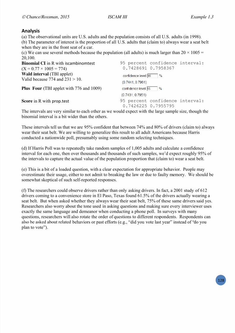
7/25/2019 Text: Investigating Statistical Concepts, Applications, and Methods
http://slidepdf.com/reader/full/text-investigating-statistical-concepts-applications-and-methods 129/428

7/25/2019 Text: Investigating Statistical Concepts, Applications, and Methods
http://slidepdf.com/reader/full/text-investigating-statistical-concepts-applications-and-methods 130/428
Chance/Rossman, 2015 ISCAM III Chapter 1 Summary
W!V
).<9!/@ H 01BB<@_
In this chapter, you have focused on making inferences based on a representative sample from a random process that can be repeated indefinitely under identical conditions or from a finite population, for asingle binary variable. You have learned how to model the chance variation in the binary outcomes that
arise from such a sampling process. You utilized simulation as a powerful tool for assessing the behavior of the outcomes and
estimating the likelihood of different results for the sample proportion. In particular, you saw youcould estimate the p-value of a test to measure how unlikely we are to get a sample proportion atleast as extreme as what was observed under certain conjectures (the null hypothesis) about the
process or population from which the sample was drawn. Then you used the binomial distribution to calculate one-sided and two-sided p-values exactly. As a third alternative for estimating p-values and confidence intervals, you considered the
normal approximation to the binomial distribution (the Central Limit Theorem for a sample proportion). In this case, we also found z-score values ( test statistics ). These are informative inaccompanying p-value calculations to provide another assessment of how unusual an observation
is. We often flag an observation as surprising or unusual if the |z-score| value exceeds 2.In each case, when the p-value is small, we have evidence that the observed result did not happen solelydue to the random chance inherent in the sampling process (a “statistically significant result”). Thesmaller the p-value, the stronger the evidence against the null hypothesis.
Still, we must keep in mind that we are merely measuring the strength of evidence we may be makinga mistake whenever we decide whether or not to reject a null hypothesis. If we decide the observedresult did not happen by chance and so reject the null hypothesis, there is still a small probability that thenull hypothesis is true and that the observed result did occur by chance (the probability of committing aType I error ). If we decide the result did happen by chance, there is still a probability that somethingother than random chance was involved (a Type II error ). It is important to consider the probabilities of
these errors when completing your assessment of a study. In particular, the sample size of the study caninfluence the probability of a Type II error and the related idea of power , which is the probability ofcorrectly rejecting a null hypothesis when it is false.
You began your study of confidence intervals as specifying an interval of plausible values for the process probability based on what you observed in the sample. These were the hypothesized parametervalues that generated two-sided p-values above the level of significance . In other words, they werethe parameter values for which your sample result would not be surprising. When the sample size islarge (large enough for the normal approximation to be valid), we saw that these confidence intervalshave a very convenient form: statistic + margin-of-error where margin-of-error = critical value ! standard error of statistic. The critical value is the number of standard errors you want to use
corresponding to a specified confidence level. Keep in mind that the level of confidence provides ameasure of how reliable the procedure will be in the long-run (which can vary by procedure and sampleconditions).
Finally, you saw that this reasoning process holds equally well when the sampling is from a finite population, where the randomness in our model comes from the selection of the observational units, notin the observational units’ individual outcomes. Here we took a bit more care to convince ourselves thatthe sample will be representative of the larger population. This is done by using random mechanisms to

7/25/2019 Text: Investigating Statistical Concepts, Applications, and Methods
http://slidepdf.com/reader/full/text-investigating-statistical-concepts-applications-and-methods 131/428

7/25/2019 Text: Investigating Statistical Concepts, Applications, and Methods
http://slidepdf.com/reader/full/text-investigating-statistical-concepts-applications-and-methods 132/428

7/25/2019 Text: Investigating Statistical Concepts, Applications, and Methods
http://slidepdf.com/reader/full/text-investigating-statistical-concepts-applications-and-methods 133/428

7/25/2019 Text: Investigating Statistical Concepts, Applications, and Methods
http://slidepdf.com/reader/full/text-investigating-statistical-concepts-applications-and-methods 134/428
Chance/Rossman, 2015 ISCAM III Chapter 1 Summary
W##
a487Q @%(%:%*7% +' M0)<B @ `':Q,?"7% L4*7+8'*, 8* )="?+%: H O0D K"*%\N%+"EPProbability (or z-score) Desired Function Name(options)*
Binomial Probability
Right tail probability of Binomial random variable X, P(X > k | ) iscambinomprob(k, n, pi, FALSE)
Left tail probability of Binomial random variable X, P(X < k | ) iscambinomprob(k, n, pi, TRUE)
Exact Binomial Test and Confidence Interval
Right/Left tail probability of Binomial random variable X, P(X > k | )iscambinomtest(k, n, pi, "greater")iscambinomtest(k, n, pi, "less")
Two-tailed probability in Binomial distribution, P(X < k or X > k2 | )w/ method of small P-values iscambinomtest(k, n, pi, "two.sided")
95% (two-sided) Binomial confidence interval iscambinomtest(k, n, conf.level = c(90, 95))
Normal Probability
Right/Left tail probability of Normal random variable X, P(X > x | , ) iscamnormprob(x, mu, sigma, "above", "x-axis-label")iscamnormprob(x, mu, sigma, "below", "x-axis-label")
Two-tailed probabilities in Normal distribution, P(X < x1 or X > x2 | , ) iscamnormprob(x1, mu, sigma, "outside", "x-axis-label", x2)
Probability between two values in Normal distribution, P(x1 < X < x2 | , ) iscamnormprob(x1, mu, sigma, "between", "x-axis-label", x2)
Inverse Normal Probability
z-score value with stated probability above/ below iscaminvnorm(probability, direction = "above")iscaminvnorm(probability, direction = "below")
z-score value with stated probability outside iscaminvnorm(probability, direction = "outside")
z-score value with stated probability between iscaminvnorm(probability, direction = "between")
Normal (z-test) Approximation for One Proportion and Confidence Interval (CI)
Right/Left tail probability of a proportion using Normal z-test, P( pˆ
> k/n | ) iscamonepropztest(k, n, pi, "greater")iscamonepropztest(k, n, pi, "less")
Two-tailed probability using Normal z-test, P( pˆ
< k/n or pˆ
> (1- k)/n | ) iscamonepropztest(k, n, pi, "two.sided")
95% (two-sided) Normal confidence interval iscamonepropztest(k, n, conf.level = c(90, 95))
* In addition to numerical output these functions provide a graphical representation.

7/25/2019 Text: Investigating Statistical Concepts, Applications, and Methods
http://slidepdf.com/reader/full/text-investigating-statistical-concepts-applications-and-methods 135/428

7/25/2019 Text: Investigating Statistical Concepts, Applications, and Methods
http://slidepdf.com/reader/full/text-investigating-statistical-concepts-applications-and-methods 136/428
Chance/Rossman, 2015 ISCAM III Chapter 2
W#R
CHAPTER 2: ANALYZING QUANTITATIVE DATA
This chapter parallels the previous one in many ways. The difference here is that these investigationswill involve a quantitative variable rather than a categorical one. This requires us to learn different toolsfor graphing and summarizing our data, as well as for statistical inference. In the end, you will find that
the basic concepts and principles that you learned in Chapters 1 still apply.
Section 1: Descriptive StatisticsInvestigation 2.1: Birth weights – Normal model, Assessing model fitInvestigation 2.2: How long can you stand it? – Skewed dataInvestigation 2.3: Cancer pamphlets - Application
Section 2: Inference for MeanInvestigation 2.4: The Ethan Allen – Sampling distributions for x Investigation 2.5: Healthy body temperatures – One-sample t -proceduresProbability Detour: Student’s t Distribution
Investigation 2.6: Healthy body temperatures (cont.) – Prediction intervalsSection 3: Inference for Other Statistics (optional)Investigation 2.7: Water oxygen levels – Sign testInvestigation 2.8: Turbidity – t -procedures with transformed dataInvestigation 2.9: Heroin treatment times - Bootstrapping
Example 2.1: Pushing On – One-sample t -proceduresExample 2.2: Distracted Driving? – Sign test
! " # $ % & ' ( ) & ' " (
+ & ) & ' % & ' , ) -
. / " , $ 0 & % 1
2 0 0
- ' , ) & ' / " % 1 ) "
3 4 $ & 5 / 3 %

7/25/2019 Text: Investigating Statistical Concepts, Applications, and Methods
http://slidepdf.com/reader/full/text-investigating-statistical-concepts-applications-and-methods 137/428

7/25/2019 Text: Investigating Statistical Concepts, Applications, and Methods
http://slidepdf.com/reader/full/text-investigating-statistical-concepts-applications-and-methods 138/428
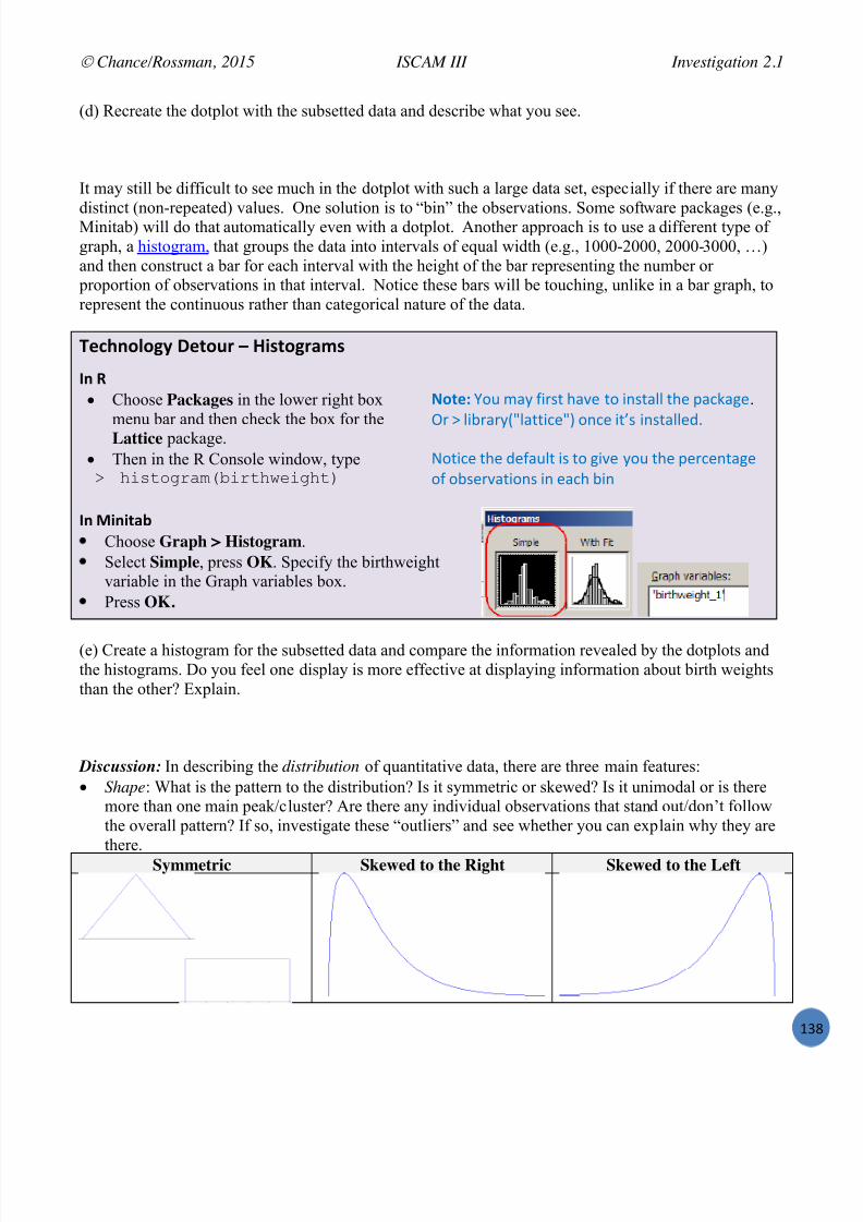
7/25/2019 Text: Investigating Statistical Concepts, Applications, and Methods
http://slidepdf.com/reader/full/text-investigating-statistical-concepts-applications-and-methods 139/428
Chance/Rossman, 2015 ISCAM III Investigation 2.1
W
(d) Recreate the dotplot with the subsetted data and describe what you see.
It may still be difficult to see much in the dotplot with such a large data set, especially if there are many
distinct (non- repeated) values. One solution is to “bin” the observations. Some software packages (e.g.,Minitab) will do that automatically even with a dotplot. Another approach is to use a different type ofgraph, a histogram, that groups the data into intervals of equal width (e.g., 1000-2000, 2000- 3000, …)and then construct a bar for each interval with the height of the bar representing the number or
proportion of observations in that interval. Notice these bars will be touching, unlike in a bar graph, torepresent the continuous rather than categorical nature of the data.
!%7=*'$'>6 2%+'4: – .8,+'>:";,
M* @ Choose Packages in the lower right box
menu bar and then check the box for theLattice package.
3'+%I D12 *&6 9'5(% +&4, %1 '.(%&-- %+, 8&)>&3,.Or > library("lattice") once it’s installed.
Then in the R Console window, type . 6?97CD3B0&L?376>;?D67*
]1%'), %+, ;,9&2-% '( %1 3'4, 612 %+, 8,5),.%&3,19 1=(,54&%'1.( '. ,&)+ ='.
M* B8*8+"# Choose Graph > Histogram . Select Simple , press OK . Specify the birthweight
variable in the Graph variables box. Press OK.
(e) Create a histogram for the subsetted data and compare the information revealed by the dotplots andthe histograms. Do you feel one display is more effective at displaying information about birth weightsthan the other? Explain.
Discussion: In describing the distribution of quantitative data, there are three main features: Shape : What is the pattern to the distribution? Is it symmetric or skewed? Is it unimodal or is there
more than one main peak/cluster? Are there any individual observations that stan d out/don’t followthe overall pattern? If so, investigate these “outliers” and see whether you can explain why they arethere.
Symmetric Skewed to the Right Skewed to the Left

7/25/2019 Text: Investigating Statistical Concepts, Applications, and Methods
http://slidepdf.com/reader/full/text-investigating-statistical-concepts-applications-and-methods 140/428
Chance/Rossman, 2015 ISCAM III Investigation 2.1
W#V
Center : Where is the distribution centered or clustered? What are typical values? Variability : How spread out is the distribution? How far do the observations tend to fall from the
middle of the distribution? What is the overall range (max – min) of the distribution?It is also very important to note any observations that do not follow the overall pattern (e.g, “outliers”)as they may reveal errors in the data or other important features to pay attention to.
(f) How would you characterize the shape, center, and variability of these birthweights? (Remember to put your comments in context, e.g., “The distribution of January birthweights in 2013 was …”)
(g) You may have noticed a few more lower weight babies than we might have expected (if we assume a“random” biological characteristic will be pretty symmetric and bell-shaped). Can you suggest anexplanation for the excess of lower birth weights seen in this distribution?
(h) Now, further subset the births2 data based on whether or not the pregnancy lasted at least 37 weeks(i.e., full_term = 1). Note: full_term values of 2 indicate missing values for this variable.[ R Hints : use “ !! ” for an equality comparis on or be clever in your inequality. Attach and use4;<D76&L?376>;?D67* to count observations.]How many observations do you end up with?
(i) After this step do we have a more symmetric distribution? What is a downside to subsetting thedataset in this way?
Let’s use this as our final dataset and use technology to calculate some helpful numerical summaries ofthe distribution, namely describing the center and variability.
!%7=*'$'>6 2%+'4: – 34;%:87"$ 04;;":8%, M* @. B77BI6&L?3769(* L5 2(, ='5%+(#e='5%+<,'3+% . ?9IB09200B31&L?376>;?D67Q A?D?79!]*f.%,5'.3 “digits = ” (8,)'9',( %+, .2*=,5 19 ('3.'9')&.% ;'3'%( 612 <&.% ;'(8-&6,;/ E,9&2-% '( #/
M* B8*8+"# Choose Stat > Basic Statistics > Display Descriptive Statistics . Specify the birthweight variable in the Variables box Optional : Under Statistics you can choose which numbers are calculated.
(j) Calculate and interpret the mean and the standard deviation of these data.

7/25/2019 Text: Investigating Statistical Concepts, Applications, and Methods
http://slidepdf.com/reader/full/text-investigating-statistical-concepts-applications-and-methods 141/428
Chance/Rossman, 2015 ISCAM III Investigation 2.1
W
(k) How would the mean and standard deviation compare if we had not removed the 9999 values?
Recall from Chapter 1 the normal probability distribution has some very nice properties and allows us to predict the behavior of our variable. For example, we might want to assume birth weights follow a
normal distribution and estimate how often a baby will be of low birth weight (under 2500 gramsaccording to the International Statistical Classification of Diseases, 10 th revision , World HealthOrganization, 2011) based on these data.
(l) Do these birth weight data appear to behave like a normal distribution? How are you deciding?
<,,%,,8*> B'5%$ L8+Many software programs will allow you to overlay a theoretical normal distribution to see how well itmatches your data, using the mean and standard deviation from the observed data.
(m) Overlay a normal model on the distribution of birthweight data and comment on how well the modelfits the data.
M* @. ?9IB0BAA<C30&L?376>;?D67* J'-- %&>, & 9,< (,)1.;( %1 &88,&5
M* B8*8+"#Right click on the graph and choose Add > Distribution Fit. Because the defaultdistribution is Normal, press OK .
Discuss any deviations from the pattern of a normal distribution.
Another method for comparing your data to a theoretical normal distribution is to see whether certain properties of a normal distribution hold true. In Chapter 1, you learned that 95% of observations in anormal distribution should fall within two standard deviations of the mean.
(n) Calculate the percentage of the birthweights that fall within 2 standard deviations of the mean bycreating a Boolean (true/false) variable:
M* @. >?76?<#9A ! &L?376>;?D67 . 0;B<&L?376>;?D67* )
#+9A&L?376>;?D67** l &L?376>;?D67 j 0;B<&L?376>;?D67* m#+9A&L?376>;?D67**
. 7BL4;&>?76?<#9A* M* B8*8+"#
Choose Calc > Calculator , store result in >?76?<#9A ,expression : I# . &0;B<&I#*)#+97A;H&I#**l I#j&0;B<&I#*m#+97A&I#**Press OK . A “1” indicates the statement is true, a “0” indicates the statement is false.
Now choose Stat > Tables > Tally Individual Variables and specify the new variable. Checkthe N12.%( and O,5),.%( boxes. Press OK .

7/25/2019 Text: Investigating Statistical Concepts, Applications, and Methods
http://slidepdf.com/reader/full/text-investigating-statistical-concepts-applications-and-methods 142/428
Chance/Rossman, 2015 ISCAM III Investigation 2.1
WPW
(o) How well does this percentage match to what would be predicted if the data were behaving like anormal distribution?
Another way to assess the “fit” of a probability model to the data is with a “probability plot” (akaquantile plot). Probability plots work roughly like this: The computer determines how manyobservations are in the data set, and then reports the z-scores it would expect for the 1/ n th percentiles for(also called quantiles ) for the probability model. The plot compares these z-scores to the observed data;if they “line up” then the graph supports that the data are behaving like a normal distribution. Whetheror not the observations follow a line can be easier to judge than whether a histogram follows a curve.
(p) Use technology to create a normal probability plot for the subsetted birth weight data. M* @
. \\<C30&L?376>;?D67Q AB7B[!U* ”datax” puts observed values on x :&B'( M* B8*8+"#
Choose Graph > Probability Plot , Single , press OK , specify the column of subsetted birthweights in the Graph variables box, and press OK .
Do the observations deviate much from a line? If so how? [ Hints: What does this suggest about how the birth weight data values differ from what we would predict for a normal distribution (e.g., smallestvalues are smaller than expected or larger than expected)? Is this consistent with what you saw in thehistogram?]
Discussion: Some software packages report a p-value with the normal probability plot. The nullhypothesis here is actually that the data do follow a normal distribution, so if you fail to reject this null
hypothesis you can say that the data do not provide strong evidence that they do not arise from anormally distributed population. (But keep in mind that large sample sizes will drive the p-value down,regardless of the actual shape of the population.) There are several different types of significance testsfor normality, but in this text we will focus on the visual judgement of whether the probability plotappears to follow a straight line.
Suppose we were willing to assume that in general birth weights are approximately normally distributedwith mean 3330 grams and standard deviation 475 grams. We can use this model to make predictions,like how often a baby will be of low birth weight , defined as 2500 grams or less.
(q) Use technology (e.g., Technology Detour with Investigation 1.8) to calculate the normal distribution
probability that a randomly selected baby will be of low birth weight. Include a well-labeled sketch withthe shaded area of interest.

7/25/2019 Text: Investigating Statistical Concepts, Applications, and Methods
http://slidepdf.com/reader/full/text-investigating-statistical-concepts-applications-and-methods 143/428

7/25/2019 Text: Investigating Statistical Concepts, Applications, and Methods
http://slidepdf.com/reader/full/text-investigating-statistical-concepts-applications-and-methods 144/428
Chance/Rossman, 2015 ISCAM III Investigation 2.2
WP#
Investigation 2.2: How Long Can You Stand It?
Diekmann, Krassnig, and Lorenz (1996) conducted a field study to explore whether drivercharacteristics are related to an aggressive response (Thanks to Jeff Sklar for pointing us to this article).The study was conducted at a busy intersection in Munich, West Germany, on two afternoons (Sunday
and Monday) in 1986. The experimenters sat in a Volkswagge n Jetta (the “blocking car”) and did notaccelerate after the traffic light turned green, and timed how long before the blocked car driver reacted(either by honking or flashing headlights). The response time (in seconds) is our variable of interest.Some values were “censored” in that the researcher stopped timing before the driver actually honked.This can happen if there is a time limit to the observation period and “success” has not been observedwithin that time period.
(a) How long do you think you would wait before you honked?
(b) The data can be found in +1.>'.3/%B%/ Use technology to create a histogram and describe the
behavior of the data – shape, center, spread, outliers (suggest an explanation?). Then overlay a normal probability model. Do these data behave like a normal distribution? If not, how do they deviate fromnormality? Also examine a normal probability plot and discuss how deviations from the line correspondto the normal name shape you are observing. [ Hint : Were the observed response times/quantiles placedon the vertical or the horizontal axis?]
(c) Compare the mean and median weight times. Which is larger? Why is it larger?
Definition: A numerical summary (statistic) is said to be resistant when it is not strongly influenced by achange in one or two extreme data values.When data are skewed to the right, the mean will be pulled in the direction of the larger values.
When data are skewed, we might often prefer to report the median as a “typical” value in the data set,rather than the mean which is pulled in the direction of the longer tail. In addition, you might not wantto cite the standard deviation as a “symmetric” measured of spread in the distribution.
Definition: Interquartile range (IQR) = upper quartile – lower quartile The lower quartile is a value such that roughly one-fourth of all the observations fall below it; the upperquartile is a value such that roughly one-fourth of all the observations fall above it. The IQR thenmeasures the width of the interval containing the middle 50% of the observations.
(d) Use technology to compute the interquartile range ( Hint : Run the descriptive statistics command andreport the lower and upper quartiles and then subtract). Write a one-sentence interpretation of this value.Would you consider it a resistant measure of spread? Explain.

7/25/2019 Text: Investigating Statistical Concepts, Applications, and Methods
http://slidepdf.com/reader/full/text-investigating-statistical-concepts-applications-and-methods 145/428

7/25/2019 Text: Investigating Statistical Concepts, Applications, and Methods
http://slidepdf.com/reader/full/text-investigating-statistical-concepts-applications-and-methods 146/428

7/25/2019 Text: Investigating Statistical Concepts, Applications, and Methods
http://slidepdf.com/reader/full/text-investigating-statistical-concepts-applications-and-methods 147/428
Chance/Rossman, 2015 ISCAM III Investigation 2.2
W
M* B8*8+"#Right click on the histogram of response times and choose Add > Distribution Fit . From theDistribution pull-down menu, select Exponential. Press OK . Or when creating a probability
plot, press the Distributions button and select Exponential.Describe the behavior of the exponential distribution. Does it appear to be a reasonable fit for these
data? Describe any deviations.
(k) Use technology to calculate the probability of a wait time under 2 seconds using the exponentialdistribution with mean 4.25 sec
M* @. 8;[8&#Q 3B7; ! ,$]=#_* OF^ g !G <+,. ^ fB8F*,&. _ P/!RG M* B8*8+"#
Choose Graph > Probability Distribution Plot. Select View Probability . Use the pull-down Distribution menu to select Exponential . Enter a scale parameter of 4.25. Under
Shaded Area select an X value of 2 and Left Tail.How does it compare to your estimate in (h) and the result in (i)?
(l) Repeat (j) and (k) with a “lognormal” distributio n. M* @
. \\84C7&3;98C<9;7?0;Q \4<C30&88C?<79&,#***
. ?9IB0AA4<C30&3;98C<9;7?0;*
. 84<C30&#Q 0;B<4CD ! (=(a(Q 9A4CD ! -=_#a_* M* B8*8+"#
Choose the Lognormal distribution with location 1.282 and scale 0.5285. Note: This is equivalent to fitting the normal distribution on the log-transformed data!
Discussion: There are of course, many other probability models we could look into. One limitation ofthe exponential distribution is assuming the mean and standard deviation are equal, clearly not the casefor these data. There are other more flexible distributions (e.g., Gamma and Weibull) that use two
parameters to characterize the distribution rather than only one.
(m) To what population are you willing to generalize these results? Explain. [ Hint : Think about how thedata were collected and what you learned about sampling methods in Chapter 1.]
(n) If you were to continue to explore this research area/ data set, what would you be interested ininvestigating next?

7/25/2019 Text: Investigating Statistical Concepts, Applications, and Methods
http://slidepdf.com/reader/full/text-investigating-statistical-concepts-applications-and-methods 148/428
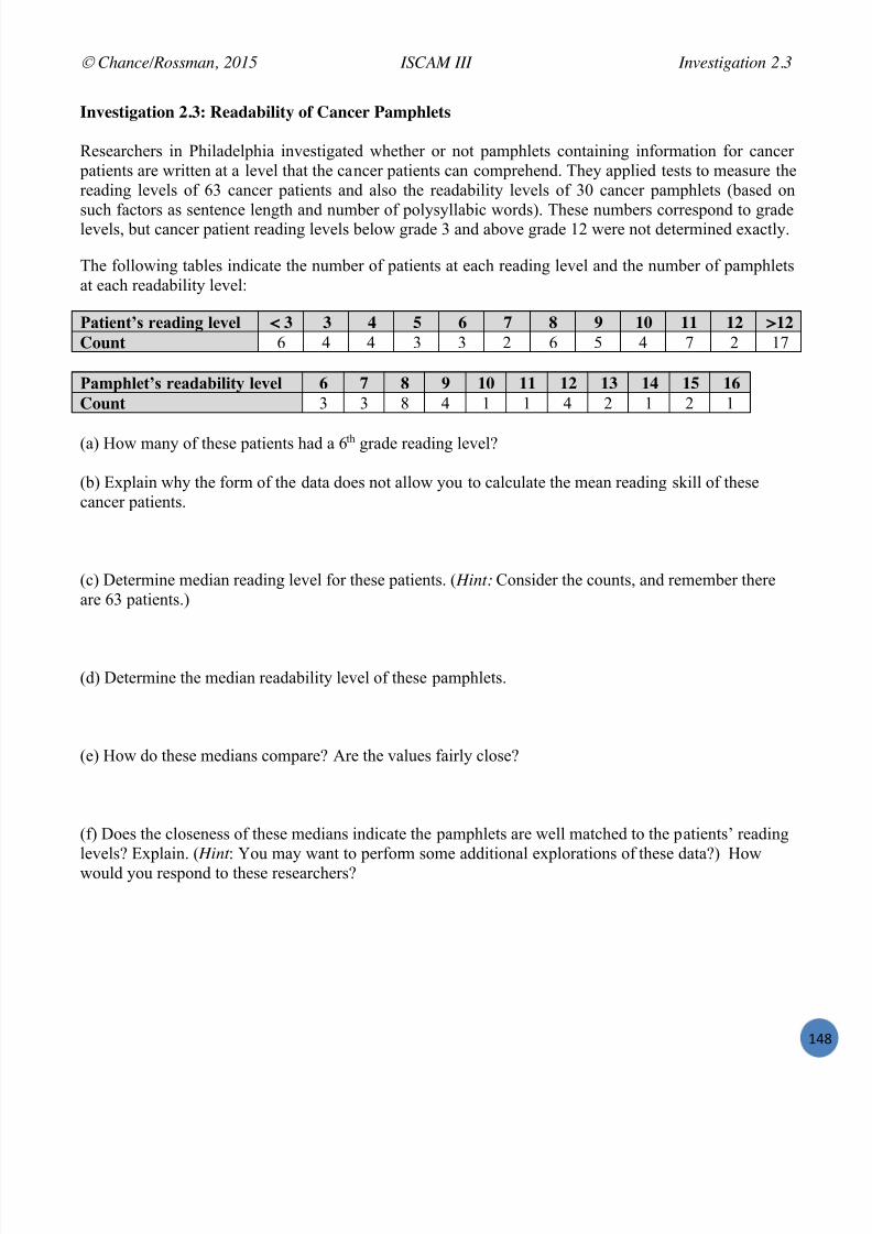
7/25/2019 Text: Investigating Statistical Concepts, Applications, and Methods
http://slidepdf.com/reader/full/text-investigating-statistical-concepts-applications-and-methods 149/428

7/25/2019 Text: Investigating Statistical Concepts, Applications, and Methods
http://slidepdf.com/reader/full/text-investigating-statistical-concepts-applications-and-methods 150/428

7/25/2019 Text: Investigating Statistical Concepts, Applications, and Methods
http://slidepdf.com/reader/full/text-investigating-statistical-concepts-applications-and-methods 151/428
Chance/Rossman, 2015 ISCAM III Investigation 2.4
W
SECTION 2: INFERENCE FOR POPULATION MEAN
In the previous section, you transitioned from categorical data to quantitative data. We started bylooking at graphs and numerical characteristics of the distribution, and here, we found that looking atthe variability of the distribution was often quite an important feature. With proportions, the sampleproportion tells us everything about the shape, center, and variability of the sample distribution. But withquantitative data we will need to consider all three of these characteristics, as well as possible outliersand other unusual observations (e.g., clustering). But often, like in Chapter 1, we want to makeinferences beyond our sample data to a larger population or process. In particular, with the Gettysburg
Address data, we saw that there is also a very predictable pattern to how sample means vary fromrandom sample to random sample, allowing us to estimate how close we expect our observed statistic(e.g., the sample mean) to be to the unknown population parameter (e.g, the population mean). We willnow further explore these theoretical results before considering other types of parameters as well (e.g.,the population median). The reasoning will be very similar but we will need to consider a newprobability model to take into account that we will also be estimating the variability in our quantitativevariable.
Investigation 2.4: The Ethan Allen
On October 5, 2005, a tour boat named the Ethan Allen capsized on Lake George in New York with 47 passengers aboard. In the inquiries that followed, it was suggested that the tour operators should haverealized that the combined weight of so many passengers was likely to exceed the weight capacity of the
boat. Could they have predicted this?
(a) The variable of interest in this study is weight of a passenger . For a sample of 47 passengers, make aconjecture as to the distribution (shape, center, variability) of this variable. Include a well-labeled sketchof your conjecture below (e.g., 47 dots or sketch an outline of the general pattern). Include a guess of thevalues of the sample mean x and the sample standard deviation s. [ Hint : Think about the size of atypical deviation from the mean, as well as the Empirical (95%) Rule.]
(b) Data from the Centers for Disease Control and Prevention indicate that weights of American adultsin 2005 had a mean of 167 pounds and a standard deviation of 35 pounds. (To convey that these are
population values, we will use Greek letters to represent their values, = 167 and = 35.) Use thisinformation to sketch a possible distribution of the weights of the population of adult Americans.
The maximum weight capacity of passengers that the Ethan Allen could accommodate was estimated to be 7500 pounds. If the tour boat company consistently accepted 47 passengers, what we want to knowis the probability that the combined weight of the 47 passengers would exceed this capacity.

7/25/2019 Text: Investigating Statistical Concepts, Applications, and Methods
http://slidepdf.com/reader/full/text-investigating-statistical-concepts-applications-and-methods 152/428
Chance/Rossman, 2015 ISCAM III Investigation 2.4
WRW
(c) What are the observational units and variable for this research question? Is this variable quantitativeor categorical? [ Hint : Notice that the probability of interest does not pertain to individual passengers.]
(d) Instead of focusing on the total weight of the 47 passengers, we can instead work with the average weight of the 47 passengers. Complete the following to indicate how these are equivalent:
Total weight of passengers > 7500 lbs when average weight of 47 passengers > .
So, to see how often the boat was sent out with too much weight, we need to know about the distributionof the average weight of 47 passengers from different boats (samples). Think about a distribution ofsample mean weights from different random samples of 47 passengers, selected from the population ofadult Americans.
(e) Where do you think the distribution of sample means will be centered?(f) Do you think the distribution of sample means would have more variability, less variability, or thesame variability as weights of individual people? Explain your answer.
(g) Do you think the probability of having the average weight exceed 159.574 pounds is larger orsmaller than the probability of the weight of any one passenger exceeding 159.574 pounds?
To investigate this probability, we will generate random samples from a hypothetical population ofadults’ weights. Open the WeightPopulations.xls data file and pretend each column is a different
population of 20,000 adult tourists, each with a population mean weight ( ) of 167 lbs and a populationstandard deviation ( ) of 35 lbs. Copy the data in the first column (818W) to the clipboard
and then open the Sampling from Finite Population applet: Press Clear , Click inside the Paste population data box, and paste the data from the clipboard. Press
Use Data .
(h) Describe the shape, mean ( ) and standard deviation( ) of this population distribution (shown in the histogram
below the window).
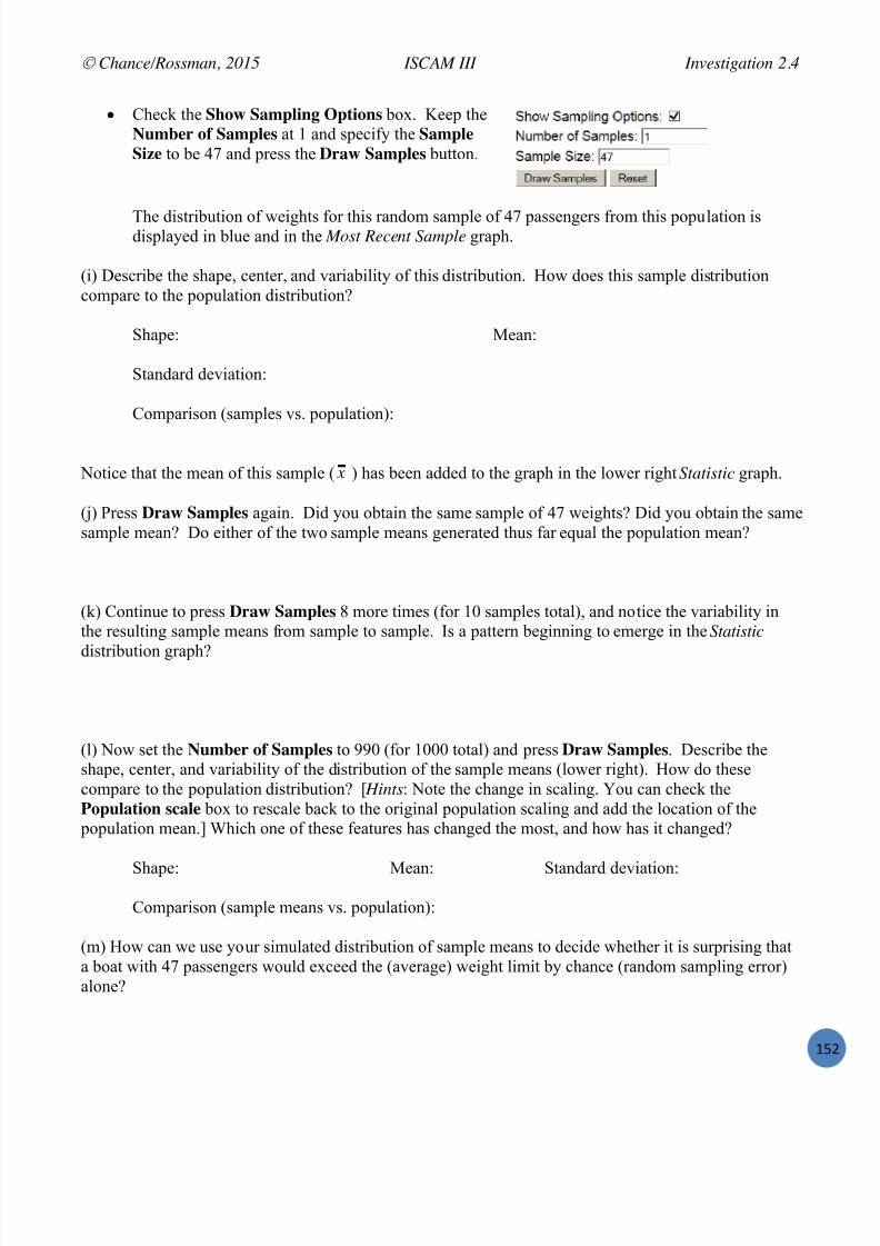
7/25/2019 Text: Investigating Statistical Concepts, Applications, and Methods
http://slidepdf.com/reader/full/text-investigating-statistical-concepts-applications-and-methods 153/428
Chance/Rossman, 2015 ISCAM III Investigation 2.4
W
Check the Show Sampling Options box. Keep theNumber of Samples at 1 and specify the SampleSize to be 47 and press the Draw Samples button.
The distribution of weights for this random sample of 47 passengers from this population isdisplayed in blue and in the Most Recent Sample graph.
(i) Describe the shape, center, and variability of this distribution. How does this sample distributioncompare to the population distribution?
Shape: Mean:
Standard deviation:
Comparison (samples vs. population):
Notice that the mean of this sample ( ) has been added to the graph in the lower right Statistic graph.
(j) Press Draw Samples again. Did you obtain the same sample of 47 weights? Did you obtain the samesample mean? Do either of the two sample means generated thus far equal the population mean?
(k) Continue to press Draw Samples 8 more times (for 10 samples total), and notice the variability inthe resulting sample means from sample to sample. Is a pattern beginning to emerge in the Statistic
distribution graph?
(l) Now set the Number of Samples to 990 (for 1000 total) and press Draw Samples . Describe theshape, center, and variability of the distribution of the sample means (lower right). How do thesecompare to the population distribution? [ Hints : Note the change in scaling. You can check thePopulation scale box to rescale back to the original population scaling and add the location of the
population mean.] Which one of these features has changed the most, and how has it changed?
Shape: Mean: Standard deviation:
Comparison (sample means vs. population):
(m) How can we use your simulated distribution of sample means to decide whether it is surprising thata boat with 47 passengers would exceed the (average) weight limit by chance (random sampling error)alone?
x

7/25/2019 Text: Investigating Statistical Concepts, Applications, and Methods
http://slidepdf.com/reader/full/text-investigating-statistical-concepts-applications-and-methods 154/428
Chance/Rossman, 2015 ISCAM III Investigation 2.4
WR#
(n) To investigate the question posed in (m), specify the sample mean of interest (159.574) in the CountSample box, use the pull-down menu to specify whether you want to count samples Greater Than , LessThan , or Beyond (both directions). Press Count . What conclusions can you draw from this count?
3'*\*':;"$ 9'?4$"+8'*To carry out the preceding simulation analysis, we assumed that the population distribution had a normalshape. But what if the population of adult weights has a different, non-normal distribution? Will thatchange our findings?
(o) Now copy and paste t he data from the “ 818! ” column in the WeightPopulations.xls data file.Describe the shape of this population and what it means for the variable to have this shape in thiscontext. How do the values of and compare to the previous population?
Shape: Mean: Standard deviation:
Comparison:
(p) Generate 1000 random samples of 47 individuals from this population. Produce a well-labeledsketch of the distribution of sample means below and note the values for the mean and standarddeviation. How does this distribution compare to the one in (l)?
Sketch: Mean:
SD:
Comparison:
(q) Again use the applet to approximate the probability of obtaining a sample mean weight of at least159.574 lbs for a random sample of 47 passengers from this population. Has this probability changedconsiderably with the change in the shape of the distribution of the population of weights?
(r) Repeat this analysis using the other population distribution (818# ) in the data file and summarizeyour observations for the three populations in the table below.
Distribution of sample means Shape Mean Standard deviationNormal ( = 167, = 35)Skewed right ( = 167, = 35)Uniform ( a = 106.4, b = 227.6)

7/25/2019 Text: Investigating Statistical Concepts, Applications, and Methods
http://slidepdf.com/reader/full/text-investigating-statistical-concepts-applications-and-methods 155/428
7/25/2019 Text: Investigating Statistical Concepts, Applications, and Methods
http://slidepdf.com/reader/full/text-investigating-statistical-concepts-applications-and-methods 156/428

7/25/2019 Text: Investigating Statistical Concepts, Applications, and Methods
http://slidepdf.com/reader/full/text-investigating-statistical-concepts-applications-and-methods 157/428
Chance/Rossman, 2015 ISCAM III Investigation 2.4
W
0+456 )'*7$4,8'*,Assuming the CDC values for the mean and standard deviation of adult Americans’ weights, μ = 167 lbsand σ = 35 lbs, we believe that the distribution of sample mean weights will be well modeled by anormal distribution (based both on the not extremely skewed nature of the variable and the moderatelylarge sample size of 47, which is larger than 30). Therefore, the Central Limit Theorem allows us to
predict that the distribution of x is approximately normal with mean 167 lbs and standard deviation35/ 47 ≈ 5.105 lbs. From this information , assuming the CDC data is representative of the populationof Ethan Allen travelers, we can estimate the probability of obtaining a sample mean of 159.57 poundsor higher to be 0.9264. Therefore, it is not at all surprising that a boat carrying 47 American adultscapsized. In fact, the surprising part might be that it didn’t happen sooner!
9:"7+87% 9:'#$%; RDU<(a) Use the Sampling from Finite Population applet or the Central Limit Theorem to estimate the
probability that the sample mean of 20 randomly selected passengers exceeds 159.57lbs, assuming anormal population with mean 167lbs and standard deviation 35lbs.
(b) Is the probability you found in (a) larger or smaller than the probability you found for 47 passengers?Explain why your answer makes intuitive sense.(c) Repeat (a) assuming a uniformly distributed population of weights. How do these two probabilitiescompare? [ Hint : Think about whether it is more appropriate to use the Sampling from Finite Populationapplet or the CLT to answer this question.](d) Explain why the calculation in (a) does not estimate the probability of the Ethan Allen sinking with20 passengers.
9:"7+87% 9:'#$%; RDUCUse the Sampling from Finite Population applet or the Central Limit Theorem to estimate the probabilitythat the sample mean of 47 randomly selected passengers would exceed 159.57lbs, assuming that
random samples are repeatedly selected from a population of 80,000 individuals with mean 167 lbs andstandard deviation 35 lbs. State any assumptions you need to make, and support your answerstatistically.

7/25/2019 Text: Investigating Statistical Concepts, Applications, and Methods
http://slidepdf.com/reader/full/text-investigating-statistical-concepts-applications-and-methods 158/428

7/25/2019 Text: Investigating Statistical Concepts, Applications, and Methods
http://slidepdf.com/reader/full/text-investigating-statistical-concepts-applications-and-methods 159/428

7/25/2019 Text: Investigating Statistical Concepts, Applications, and Methods
http://slidepdf.com/reader/full/text-investigating-statistical-concepts-applications-and-methods 160/428
Chance/Rossman, 2015 ISCAM III Investigation 2.5
WRV
So if we have a value for , we are fine. But what about the statistic suggested in (f); does thisstandardized statistic behave nicely and is this distribution again well modeled by a normal distribution?
(k) In the applet, change the Statistic option (above the graph) to t -statistic , the name for thestandardized sample mean using the standard error of the sample mean. Describe the shape of the
distribution of these standardized statistics from your 10,000 random samples.
(l) Check the box to Overlay Normal Distribution ; does this appear to be a reasonable fit? What p-value does this normal approximation produce? [ Hint : Enter your answer to (f) as the observed resultfor the t -statistic and count beyond.]
(m) Does the theory-based p-value from the normal distribution accurately predict how often we wouldsimulated a standardized statistic at least as extreme (in either direction) as the observed value of 1.73?Does it over predict or underpredict? [ Hint : How does the behavior of the distribution of thestandardized statistics most differ from a normal model?]
Discussion: If we zoom in on the tails of the distribution, we see that more of the simulated distributionlies in those tails than the normal distribution would predict.
To model the sampling distribution of the standardized statistic ( x )/(s/ n ), we need a density curvewith heavier tails than the standard normal distribution. William S. Gosset, a chemist turned statistician,showed in 1908, while working for the Guinness Breweries in Dublin, that a “t probability curve ” (seenext page) provides a better model for the sampling distribution of this standardized statistic when the
population of observations follows a normal distribution.
(n) Check the Overlay t-distribution box. What is the main visual difference in the t-distribution modelcompared to the normal distribution model? Does this t-distribution appear to be a better model for thesimulated sampling distribution? Is the theory-based p-value using the t -distribution closer to theempirical p-value than the theory-based p-value using the normal distribution?

7/25/2019 Text: Investigating Statistical Concepts, Applications, and Methods
http://slidepdf.com/reader/full/text-investigating-statistical-concepts-applications-and-methods 161/428
7/25/2019 Text: Investigating Statistical Concepts, Applications, and Methods
http://slidepdf.com/reader/full/text-investigating-statistical-concepts-applications-and-methods 162/428
Chance/Rossman, 2015 ISCAM III Investigation 2.5
WSW
But what about confidence intervals?
(p) Turn to the Simulating Confidence Intervals applet. Change the Method to Means, but keep the population set to Normal and z with . Set the population mean to 98.6, the population standarddeviation to 0.733, and the sample size to 13. Generate 1000 random samples from this population and
examine the running total for the percentage of 95% confidence intervals that successfully capture theactual value of the population mean . Is this “z with sigma” procedure behaving as it should? How areyou deciding?
(q) But more realistically, we don’t know and will use s in calculating our confidence interval.Predict what will change about the resulting confidence intervals from different random samples. [ Hint :Think of two main properties of confidence intervals.]
(r) Change the Method now to z with s . What percentage of these 1000 confidence intervals succeed incapturing the population mean of 98.6? Is this close to 95%? If not, is it larger or smaller?
(s) Repeat (r) with a sample size of n = 5.
Discussion: This “z with s” procedure produces a coverage rate (for successfully capturing the value ofthe population mean) that is less than 95%, because again the normal distribution doesn’t account for theadditional uncertainly resulting from sample to sample when we need to use both x and s. The fix will
be to multiply the standard error by a critical value larger than 1.96 to compensate for the additionaluncertainty introduced by estimating with s. The t-distribution will come to our rescue. Which t-distribution do we use? That will depend on our sample size; with smaller samples we need heavier tailsand with larger samples we need a distribution more like the normal probability model. The heaviness ofthe tails will be determined by the “degrees of freedom” of the t-distribution.
(t) Change the Method to t . How do the intervals visibly change? Is the coverage rate indeed closer to
95%?
This leads to a confidence interval formula with the same general form as the previous chapter)()( statisticof SE valuecriticalstatisticsample , where the critical value now comes from the t n – 1
(degrees of freedom = n – 1) distribution instead of the standard normal distribution.

7/25/2019 Text: Investigating Statistical Concepts, Applications, and Methods
http://slidepdf.com/reader/full/text-investigating-statistical-concepts-applications-and-methods 163/428
Chance/Rossman, 2015 ISCAM III Investigation 2.5
W
One-sample t -interval for : When we have a symmetric sample or a large sample size, anapproximate confidence interval for is given by:
nst x n /*1
Keep in mind that the critical value t * tells us how many standard errors we need to extend from thesample mean depending on how confident we want to be. Our goal is to develop a 100 ! C %confidence interval method that will capture the population parameter 100 ! C % of the time in the longrun.
(u) Find the t * value corresponding to a 95% confidence level and a sample size of n = 5 M* @I
. ?9IB0?<H7&=b_Q ]Q 5L;7>;;<5* M* B8*8+"#I
C Graph > Probability Distribution Plot > View Probability. C Select the t-distribution from the pull-down menu and set the degrees of freedom to 4. C Select Shaded Area and Define the Shaded Area By Probability. Set the Probability in Both
Tails to be .05. + 9:'#"#8$8+6 )"$74$"+': "??$%+I
C Specify 4 as the degrees of freedom C Check the box next to the less than symbol and then entire .025 in the probability box and
press Return. The t-value box should fill in.
How does this critical value compare to the corresponding z* value for 95% confidence?
t 4* = z* =
Comparison:
(v) Repeat (u) for the sample size of n = 13. How do the t -critical values compare for these differentsample sizes? Is this what you expected? Explain.
(w) Repeat (v) for the sample size of n = 130. How does this value compare to the earlier t * and z*values?
(x) Use the critical value from (w) to calculate a 95% confidence interval for the mean body temperatureof a healthy adult based on our sample ( x = 98.249, s = 0.733). Is this interval consistent with yourconclusion about the null hypothesis in (o)? Explain.

7/25/2019 Text: Investigating Statistical Concepts, Applications, and Methods
http://slidepdf.com/reader/full/text-investigating-statistical-concepts-applications-and-methods 164/428
Chance/Rossman, 2015 ISCAM III Investigation 2.5
WS#
!%7=*'$'>6 2%+'4: – -*% 0";?$% " \?:'7%54:%,
M* @, 612 )&. 2(, %+, %/%,(% )1**&.; <'%+ 5&< ;&%&(“x”) 15 '()&*1.,(&*8-,% <'%+ (2**&56 ;&%& .OR
7=7;97&[Q 02 ! B47;3<B7?H;!57>C=9?A;A5Q IC<G=4;H;4 ! =b_*
. ?9IB0C<;9B084;7&[LB3!ba=#]bQ 9A!=c((Q < !,(-Q 618C76;9?d;A !ba=^Q B47;3<B7?H; ! 57>C=9?A;A5Q IC<G=4;H;4 ! b_*where sd = sample standard deviation, s.
M* B8*8+"# Choose Stat > Basic Statistics > 1-Sample t . Specify the column of data or use the pull-down menu for
Summarized data and enter the sample size, mean, andstandard deviation.
Check the box to perform the hypothesis test and enter thehypothesized value of .
Under Options specify the direction of the alternative.(Use the two-sided option to get a confidence interval.)
Press OK twice.
M* !=%':6\C",%5 M*(%:%*7% "??$%+ Select One mean from the Scenario pull-down menu
You can check Paste data to copy and paste in the raw data, or typein the sample size, mean, and standard deviation. Press Calculate .
Check the box for Test of significance and enter the hypothesizedvalue of and set the direction of the alternative. Press Calculate .
Check the box for Confidence interval , enter the confidence leveland press Calculate CI .
(y) Verify your by-hand calculations with technology and summarize the conclusions you would drawfrom this study (both from the p-value and the confidence interval, including the population you arewilling to generalize to). Also include interpretations, in context, of your p-value and your confidencelevel.

7/25/2019 Text: Investigating Statistical Concepts, Applications, and Methods
http://slidepdf.com/reader/full/text-investigating-statistical-concepts-applications-and-methods 165/428
Chance/Rossman, 2015 ISCAM III Investigation 2.5
W
0+456 )'*7$4,8'*,The sample data provide very strong evidence that the mean body temperature of healthy adults is not98.6 degrees ( t = 5.46, two-sided p-value < 0.001). This indicates there is less than a 0.1% chance ofobtaining a sample mean as far from 98.6 as 98.249 in a random sample of 130 healthy adults from a
population with mean body temperature of 98.6 0F. A 95% confidence interval for the population mean
body temperature is (98.122, 98.376), so we can be 95% confident that the population mean bodytemperature among healthy adults is between 98.122 and 98.376 degrees. This interval is entirely lessthan 98.6, consistent with our having found very strong evidence to reject 98.6 as a plausible value forthe population mean. We are 95% confident, meaning if we were to repeat this procedure on thousandsof random samples, in the long-run roughly 95% of the resulting intervals would successfully capturethe population mean. We believe these procedures are valid because the sample size of 130 should belarge enough unless there is severe skewness or outliers in the population.
9:"7+87% 9:'#$%; RDV<Explore the last statements in the above results box using t confidence intervals:(a) Continue with the Simulating Confidence Intervals applet. Explore the coverage rate of the t -
procedure with random samples from an Exponential (skewed) population for n = 5, n = 100, and n =200. Assess and summarize the performance of this t -procedure in each case.(b) Repeat (a) for a Uniform population distribution with endpoints a = 80 and b = 85.
9:"7+87% 9:'#$%; RDVCA study conducted by Stanford researchers asked children in two elementary schools in San Jose, CA tokeep track of how much television they watch per week. The sample consisted of 198 children. Themean time spent watching television per week in the sample was 15.41 hours with a standard deviationof 14.16 hours.(a) Carry out a one-sample t -test to determine whether there is convincing evidence that average amountof television watching per week among San Jose elementary children exceeds fourteen hours per week.(Report the hypotheses, test statistic, p-value, and conclusion at the 0.10 level of significance.)(b) Calculate and interpret a one-sample 90% t -confidence interval for the population mean.(c) Comment on whether the technical conditions for the t -procedures are satisfied here. [ Hint : What canyou say based on the summary statistics provided about the likely shape of the population?]

7/25/2019 Text: Investigating Statistical Concepts, Applications, and Methods
http://slidepdf.com/reader/full/text-investigating-statistical-concepts-applications-and-methods 166/428
Chance/Rossman, 2015 ISCAM III Investigation 2.6
WSR
Investigation 2.6: Healthy Body Temperatures (cont.)
Reconsider the research question of Investigation 2.5 where a “one -sample t -test” found convincingevidence with sample mean body temperature of x = 98.249 0F and a sample standard deviation of s =0.733 0F against the hypothesis that = 98.6 in the population. In fact, we were 95% confident that
actually fell between 98.122 and 98.376 degrees (so not all that far from 98.6).
(a) So if you recorded a body temperature of 98.6 0 would you be convinced you were sick? Whattemperature values would you be concerned about?
(b) Is it true that approximately 95% of the temperatures in the sample fall inside your confidenceinterval? What percentage does? Do you think 95% of the temperatures in the population fall within theconfidence interval?
9:%587+8'* M*+%:F"$,It is very important to keep in mind that the confidence interval reported above only makes statementsabout the population mean, not individual body temperatures. But what if we instead wanted an intervalto estimate the body temperature of a single randomly selected healthy adult rather than the populationmean body temperature?
(c) Still using our same sample results, what one number would you use to predict a healthy bodytemperature? If you then considered the uncertainty (margin-of-error) in this estimate for predicting one
person’s body temperature, would you expected this margin -of-error to be larger or smaller then for predicting the population mean body temperature? Explain.
Estimate: Margin-of-error:
Explain:
To construct such a confidence inter val (often called a “prediction interval” to indicate that it will predict an individual outcome rather than the population mean), we need to consider both the sample-to-sample variation in sample means as well as the individual-to-individual variation in body temperatures.
(d) We will estimate this combined standard error of an individual value by s n/11 . Using thisformula, how will this compare to the standard error of the sample mean (larger or smaller)? Explain.
(e) Calculate this value for the body temperature data.
7/25/2019 Text: Investigating Statistical Concepts, Applications, and Methods
http://slidepdf.com/reader/full/text-investigating-statistical-concepts-applications-and-methods 167/428
7/25/2019 Text: Investigating Statistical Concepts, Applications, and Methods
http://slidepdf.com/reader/full/text-investigating-statistical-concepts-applications-and-methods 168/428
Chance/Rossman, 2015 ISCAM III Investigation 2.6
WST
0+456 )'*7$4,8'*,For one person to determine whether they have an unusual body temperature, we need a predictioninterval rather than a confidence interval for the population mean. A 95% prediction interval for the
body temperature of a healthy adult turns out to be (96.79, 99.71), a fairly wide interval. We are 95%confident that a randomly selected healthy adult will have a body temperature in this interval. This
prediction interval procedure is valid only if population of healthy body temperatures follows a normaldistribution, which seems like a reasonable assumption in this context
9:"7+87% 9:'#$%; RDY<(a) Examine the expression for a confidence interval for a population mean . What happens to the half-width of the interval as the sample size n increases? Describe its limiting behavior.(b) Examine the expression for a prediction interval for an individual observation. What happens to thehalf-width of the interval as the sample size n increases? Describe its limiting behavior.(c) Explain why the differences in your answers to (a) and (b) make sense.
9:"7+87% 9:'#$%; RDYCRecall the Stanford study on television viewing habits from Practice Problem 2.5B, with a sample sizeof 198, sample mean 15.41 and sample standard deviation 14.16.(a) Use this information to calculate a 95% prediction interval.(b) Provide a one-sentence interpretation of this interval.(c) Do you think this interval procedure is valid for these data? Explain.

7/25/2019 Text: Investigating Statistical Concepts, Applications, and Methods
http://slidepdf.com/reader/full/text-investigating-statistical-concepts-applications-and-methods 169/428
Chance/Rossman, 2015 ISCAM III Investigation 2.6
W
04;;":6 '( -*%\,";?$% " 9:'7%54:%,
Parameter: = the population mean
To test H 0: = 0
Test statistic: t 0 = ( x )/(s / n )Degrees of freedom = n 1
t -Confidence interval for x + t *n 1 s / n
Technical conditions: These procedures are considered valid if the sample distribution isreasonably symmetric or the sample size is at least 30.
Technology R: %/%,(% F;&%&7 +681%+ 7 &-%_`35,&%,5`7 `-,((`7 15 `%<1/(';,;`7 )1.9/-,4,-Gor 5&< ;&%&
'()&*1.,(&*8-,%FB=&57 (;7 .7 +681%+,('K,;7 &-%,5.&%'4,7 )1.9/-,4,-G (2**&56 ;&%& Minitab: Stat > Basic Statistics > 1-Sample t
You can paste in a column of data or input summarized data.Check the box to “Perform hypothesis test” and enter a hypothesized val ue for the
population mean. Under Options you can change the confidence level and set the direction ofthe alternative. (Use a two-sided alternative when calculating confidence intervals.)
Theory-Based Inference applet Use the pull-down menu to select One Mean . Specify the summary statistics (the samplesize, sample mean, and sample standard deviation s) or paste in the raw data. Check the
box for test of significance and specify the hypothesized value, use the button to specifythe direction of the alternative (< > for not equal) and press Calculate and/or check the
box for confidence interval, specify the confidence level and press Calculate CI.
Summary Prediction Intervals for Individual Observations
Prediction Interval: x + (t *n 1) s n/11 Valid only with normal population of observations

7/25/2019 Text: Investigating Statistical Concepts, Applications, and Methods
http://slidepdf.com/reader/full/text-investigating-statistical-concepts-applications-and-methods 170/428
Chance/Rossman, 2015 ISCAM III Investigation 2.7
WSV
SECTION 3: INFERENCE FOR OTHER STATISTICS
The previous section illustrated some very nice mathematical results for the distribution of the samplemean when sampling from an infinite process or a finite population. However, we also saw in Section 1that the mean may not be the parameter we are most interested in and/or may not even be possible tocalculate depending on the form of the data. In this section, you will look at a possible inferenceprocedure when the median is of interest, as well as a newer methodology that works for any statistic ofyour choosing.
Investigation 2.7: Water Oxygen Levels
Scientists often monitor the “health” of water systems to determine t he impact of different changes inthe environment. For example, Riggs (2002) reports on a case study that monitored the dissolvedoxygen downstream from a commercial hog operation. There had been problems at this site for severalyears (e.g., manure lagoon overflow), including several fish deaths in the previous three years justdownstream of a large swale through which runoff from the hog facility had escaped. The state pollutioncontrol agency decided to closely monitor dissolved oxygen downstream of the swale for the next threeyears to determine whether the problem had been resolved. In particular, they wanted to see whetherthere was a tendency for the dissolved oxygen level in the river to be less than the 5.0 mg/l standard.Sampling was scheduled to commence in January of 2000 and run through December of 2002. Themonitors took measurements at a single point in the river, approximately six tenths of a mile from theswale, once every 11 days.
(a) Identify the observational units in this study. Would you consider this sampling from a population orfrom a process?
(b) Because the dissolved oxygen measurements were taken in the same location at fixed time intervals,would you consider this a simple random sample? Do you think the sample is likely to be representativeof the river conditions? Explain.
Definition: A systematic sample takes selects observations at fixed intervals (e.g., every 10 th person inline). If the initial observation is chosen at random and there is no structure in the data matching up tothe interval size (e.g., every 7 th day), then such samples are generally assumed to be representative of the
population. In fact, we will often simplify the analysis by assuming they behave like simple random
samples.
(c) Examine the data from the first year in J&%,5h2&-'%6/%B%. Describe the shape, center, and variabilityof the distribution. In particular, how do the mean and median compare? Do these data appear to bewell-modelled by a normal distribution?

7/25/2019 Text: Investigating Statistical Concepts, Applications, and Methods
http://slidepdf.com/reader/full/text-investigating-statistical-concepts-applications-and-methods 171/428
Chance/Rossman, 2015 ISCAM III Investigation 2.7
W
(d) State the null and alternative hypotheses for testing whether the long-run mean dissolved oxygen inthis river is less than 5.0 mg/l (indicating too little oxygen in the water, causing problems in the aquaticcommunity structure).
(e) Is the one-sample t -test likely to be valid for these data? Explain why or why not.
(f) An alternative analysis involves recoded the ob servations as “compliant” and “not compliant.” If wesay a measurement is non-compliant when the dissolved oxygen is below 5.0 mg/l, how many non-compliant measurements do we have in this data set? What proportion of the sample is below 5.0 mg/l?[ Hint : What do you want to do with the observation that is equal to 5.0?]
(g) Carry out a test for deciding whether the proportion of measurements that fall below 5.0 mg/l isstatistically significantly larger than 0.50.
(h) If you decide that more than half of the time the river is non-compliant (that is, more than 50% ofmeasurements are below 5.0 mg/l), what does that imply about the long-run median dissolved oxygenlevel? Explain.
(i) Identify one advantage to this analysis over the one-sample t -test. Identify one disadvantage of thisanalysis over the one-sample t -test.
7/25/2019 Text: Investigating Statistical Concepts, Applications, and Methods
http://slidepdf.com/reader/full/text-investigating-statistical-concepts-applications-and-methods 172/428
Chance/Rossman, 2015 ISCAM III Investigation 2.7
WTW
(j) The researchers actually wanted to decide whether the river was non-compliant more than 10% of thetime. How would that change your analysis in (g) and would the p-value be larger or smaller?
0+456 )'*7$4,8'*,Both the mean (not shown) and of the median indicate that dissolved oxygen in this river tended to
below the 5.0 mg/l that was cited as the “action level.” Although we don’t have statistically significan tevidence that the long-run median DO level is below 5.0 (binomial p-value 0.30), the researchersactually wanted to engage in remedial action if the river is found to be in non-compliance significantlymore than 10% of the time. The exact binomial probability of observing 19 or more non-compliantvalues from a process with a 0.10 chance of non-compliance is 4.16 ! 10 -11 , leaving “little doubt that
the10% non-compliant criterion was exceeded at the monitoring site during 2000. ”
Discussion : When we use 0.50 as the hypothesized probability of success and we count how many ofour quantitative observations exceed some pre-specified level, this is called the sign test and correspondsto a test of whether the population median equals that pre-specified level. The sign test can beadvantageous over the t -test if the validity conditions for the t -test are not met (e.g., skewness in sample,not a large sample size). However, although this procedure focuses on how often you are above or belowthat level, it does not provide information about how far above or below as a confidence interval for themean could.
9:"7+87% 9:'#$%; RDZ Return to Practice Problem 2.2A. Carry out a test to determine whether there is convincing evidencethat the median student estimate of 30 seconds differs from 30. (State your hypothesis, statistic and/ortest statistic, and p-value.)

7/25/2019 Text: Investigating Statistical Concepts, Applications, and Methods
http://slidepdf.com/reader/full/text-investigating-statistical-concepts-applications-and-methods 173/428
Chance/Rossman, 2015 ISCAM III Investigation 2.8
W
Investigation 2.8: Turbidity
Another measure of water quality is turbidity, the degree of opaqueness produced in water by suspended particulate matter. Turbidity can be measured by seeing how light is scattered and/or absorbed byorganic and inorganic material. Larger nephelometric turbidity units (NTU) indicate increased turbidity
and decreased light penetration. If there is too much turbidity, then not enough light may be penetratingthe water, affecting photosynthesis to the surface and leading to less dissolved oxygen. Riggs (2002) provides 244 turbidity monthly readings (%25=';'%6/%B%) that were recorded between 1980-2000 from areach of the Mermentau River in Southwest Louisiana. The unit of analysis was the monthly meanturbidity (NTU) computed fr om each month’s systematic sample of 21 turbidity measurements. Theinvestigators wanted to determine whether the mean turbidity was greater than the local criterion valueof 150 NTU.
(a) Verify that a log-normal probability model is reasonable for these data.
(b) Carry out a log transformation and report the mean, median, and standard deviation of thetransformed data.
(c) Are the mean and median values in (b) similar to each other? Is the mean of the logged turbidityvalues similar to the log of the mean of the turbidity values? Is the median of the logged turbidity valuessimilar to the log of the median of the turbidity values?
Original scale: Transformed scale:mean = mean =
median = median =
log(mean) =log (median) =
(d) Explain why the median(log(turbidity)) is expected to be the same as log(median(turbidity)), but thisinterchangeability is not expected to work for the mean.
(e) Use a one-sample t -confidence interval to estimate the mean of the log-turbidity value for this river.
(f) Back-transform the endpoints of this interval to return to the original units.

7/25/2019 Text: Investigating Statistical Concepts, Applications, and Methods
http://slidepdf.com/reader/full/text-investigating-statistical-concepts-applications-and-methods 174/428
Chance/Rossman, 2015 ISCAM III Investigation 2.8
WT#
Discussion: Once you create a symmetric distribution, the mean and median will be similar. However,although transforming the data does not affect the ordering of the observations, it does impact thescaling of the values. So whereas the median of the transformed data is equal to taking the log of themedian of the original data (at least with an odd number of observations), this does not hold for themean. So when we back-transform our interval for the center of the population distribution, we will
interpret this in terms of the median value rather than the mean value.
0+456 )'*7$4,8'*,A 95% confidence interval based on the transformed data equals (4.20, 4.40). Therefore, we will say weare 95% confident that the median turbidity in this river is between 66.69 NTU and 81.45 NTU, clearlyless than the 150 NTU regulation. However, another condition for the validity of this procedure is thatthe observations are independent. Further examination of these data reveals seasonal trends.Adjustments need to be made to account for the seasonality before these data are analyzed.
9:"7+87% 9:'#$%; RD[ Return to the +1.>'.3/%B% data from Investigation 2.2.(a) Use the log transformation to calculate a 95% confidence interval for the mean log response time.(b) Back-transform and interpret the interval.(c) Outline a method for verifying that this procedure results in a 95% confidence interval for the
population median.

7/25/2019 Text: Investigating Statistical Concepts, Applications, and Methods
http://slidepdf.com/reader/full/text-investigating-statistical-concepts-applications-and-methods 175/428

7/25/2019 Text: Investigating Statistical Concepts, Applications, and Methods
http://slidepdf.com/reader/full/text-investigating-statistical-concepts-applications-and-methods 176/428
Chance/Rossman, 2015 ISCAM III Investigation 2.9
WTR
(c) Use technology to take a bootstrap sample from the heroin data. M* @I
. 9B084;, ! 9B084;&7?0;9Q #(aQ 3;84BI; ! UPJ'* M* B8*8+"#I
NUe. 9B084; #(a I] IcO don’t forget the semi :)1-1.
KJe". 3;84BI;= don’t forget the period Now calculate the median of your bootstrap sample. (Notice we could calculate any statistic we wanted.)
(d) Take another bootstrap sample. Did you get the same sample median? Why or why not?
To estimate the sample to sample variation in our statistic (e.g., the median), we now want to repeat this process a large number of times.(e) Use technology to create a bootstrap distribution from the heroin data.
!%7=*'$'>6 2%+'4: – C''+,+:"? 0";?$8*>
M*[ )5,&%, & -'(% 19 =11%(%5&8 (&*8-,( &.; %+,. &88-6 %+, *,;'&. %1 ,&)+ (&*8-,. 3;9B084;9 !4B8841&,:,---Q G2<I7?C<&?* 9B084;&7?0;9Q 3;84BI;!U**. LCC7973B80;A?B<9 ! 9B8841&3;9B084;9Q 0;A?B<*
M* B8*8+"# D12 *&6 <&.% %1 3,.,5&%, 1., 5,:(&*8-, =,915, '.)5,&('.3 %+, .2*=,5 19 5,:(&*8-,(Use a text editor (e.g., Tools > Notepad ) and create either a .mtb or a .mac macro:.mtb macro .mac macro9B084; #(a I] IcO3;84BI;=4;7 Ia&@,* ! 0;A?B<&Ic*4;7 @, ! @, m ,
Now save this file as "bootstrapmacro.mtb"(use the quotation marks). Make sure youkeep track of where this file goes.
Initialize k1: 4;7 @, ! ,Then select File > Other Files > Run anExec . Specify the Number of times toexecute and press Select File . Find the fileand press Open .
oNS"PheCC7973B88?<D .&*, %+, *&)51
%C @,!,:,---9B084; #(a I] IcO3;84BI;=4;7 Ia&@,* ! 0;A?B<&Ic*'<A%C'g%NS"PhThen save this file as “bootstrapmacro.mac“ (usethe quotation marks). Save this file and the Minitabworksheet in the same direction. Then to executethe file you can typeNUe. XLCC7973B80BI3C=0BI
You should now have a column of all the medians from 1000 different bootstrap samples.(f) Produce graphical and numerical summaries of the 1000 bootstrap medians. Describe the behavior ofthe bootstrap distribution.

7/25/2019 Text: Investigating Statistical Concepts, Applications, and Methods
http://slidepdf.com/reader/full/text-investigating-statistical-concepts-applications-and-methods 177/428
Chance/Rossman, 2015 ISCAM III Investigation 2.9
W
(g) Suggest a quick method for using the distribution in (d) to calculate a rough confidence interval forthe population median. Hint : Recall our usual estimate + 2 ! standard deviation of estimate . Calculateand interpret this interval.
Discussion: Once you get an estimate of the standard deviation of the statistic, there is still someconsideration of how to construct a confidence interval. In this case, the distribution of medians shouldlook fairly symmetric, so a symmetric confidence interval can work. In other cases, there are morecomplicated “adjustments” that can be made to get a bootstrap confidence interval. Discussion of thesemethods is beyond of the scope of this text, but you have seen an example of the power of bootstrapping
– you can create a distribution for any statistic that should have the same variability as the samplingdistribution of that statistic, without having to pretend you know anything about the population!
(h) Repeat this analysis, but now using the upper quartile (75% percentile) as the statistic.
M* @I. LCC7973B8\2B<7?4;9 ! 9B8841&3;9B084;9Q \2B<7?4;*. LCC973B8\2B<7?4;9iQ,k i(,, (%&%'(%')( 915 9'5(% (&*8-, . 288;3c_ ! LCC7973B8\2B<7?4;9i]E:]EQ k i(&4, h2 915 &-- 5,(&*8-,(
M* B8*8+"#: NUe. 9C37 Ic IaNUe. 4;7 Ib&@,* ! Ia&,ca*
0+456 )'*7$4,8'*,The distribution of treatment times was skewed to the right with a median of about 1 year (367.5 days)and interquartile range of 418.5 days. Because of the skewness and truncation in the data, we might
prefer the median or even the third quartile as the statistic. Based on a bootstrap simulation, anapproximate 95% confidence interval for the median treatment time in the population of heroin addictsis between 306 days and 430 days (but results will vary), while an approximate 95% confidence intervalfor the upper quartile is around 534 to 638 days (results will vary). The interval for the median includeslower values than a t -interval for the population mean (368, 437), because the t -procedure is morestrongly affected by the skewness in the data. We would like to generalize these data to all heroin
patients, but would like more information to insure that this sample is representative.
9:"7+87% 9:'#$%; RD]< (a) Apply this method to obtain an estimate of the standard deviation of the 25% trimmed mean. [ Hints :Create and sort a sample, then subset the middle 50% of the values and find the mean of those values.](b) What is an advantage to the trimmed mean compared to the mean?(c) What is an advantage to the trimmed mean over the median?
9:"7+87% 9:'#$%; RD]C Return to the +1.>'.3/%B% data from Investigation 2.2.(a) Suggest a reason why the Central Limit Theorem may not apply with these data.(b) Create and interpret an informal (+ 2SE) bootstrap confidence interval for the population median.

7/25/2019 Text: Investigating Statistical Concepts, Applications, and Methods
http://slidepdf.com/reader/full/text-investigating-statistical-concepts-applications-and-methods 178/428
Chance/Rossman, 2015 ISCAM III Example 2.1
WTT
Example 2.1: Pushing OnTry these questions yourself before you use the solutions following to check your answers.
As in many states, California mandates physical fitness testing at different grade levels. Therecommended number of push-ups for 12 year old males is 10-20 and for 13 year old males is 12-25. A
sample of 80 7th
grade males was obtained at a rural high school in Central California (Wetzel andHernandez, 2004). Data was gathered using the measurement techniques defined by the state. (The feetare together, hands will be shoulder width apart, the subjects back will be straight, and their eyes will belooking toward the horizon. The arms need to bend to a 90-degree angle, while keeping their back flat.The push-ups are counted at a set tempo without stopping to rest.)
A histogram and summary statistics of the sample data are below:
(a) Describe the distribution of the results in this sample.
(b) Suppose we take random samples of 80 males from a very large population. According to theCentral Limit Theorem, what can you say about the behavior of the sampling distribution of the samplemeans calculated from these samples?
(c) If this were a random sample from a population, would the sample data provide strong evidence thatthe population mean differs from 20 push-ups? Conduct a significance test to address this question.Also calculate confidence intervals to estimate the population mean with various levels of confidence.
(d) What precautions should we have in analyzing these results?

7/25/2019 Text: Investigating Statistical Concepts, Applications, and Methods
http://slidepdf.com/reader/full/text-investigating-statistical-concepts-applications-and-methods 179/428
Chance/Rossman, 2015 ISCAM III Example 2.1
W
(e) Would it be reasonable to use this sample to calculate a prediction interval for the number of push-ups by a 7 th grade male in California?
<*"$6,8,(a) For this sample, the distribution of the number of push-ups completed is slightly skewed to the right.The average number of push-ups by the 80 males in the sample was 15.49, with standard deviation 7.74
push-ups. Most students completed about 10-25 push-ups, with the maximum around 40 or so.(b) Because the sample size is large (80 > 30), the sampling distribution of sample means should beapproximately normal, regardless of the population shape, with mean , and standard deviation equal to
/ 80 . The exact values of (the population mean number of push-ups done by 7 th grade males) and (the population standard deviation) are unknown, but they should be in the ball park of 15.49 and 7.74,the sample statistics.(c) Test of significance : If this was a random sample from a larger population of 7 th graders, let represent the mean number of push-ups that would be completed in this population. We want to decidewhether is significantly different from 20.
H0: = 20 (the population mean number of push-ups is 20)Ha; ≠ 20 (the population mean differs from 20)
Because we are working with a quantitative response variable and the sample size is large, wewill model the sampling distribution of the standardized statistic with the t distribution with 80-1=79 degrees of freedom.
80/74.7
2049.15
/
0
ns
xt = 5.21
p-value = 2P(T 79 < 5.21) = 2(0.0000007) = 0.0000014
With such a small p-value, we easily reject the null hypothesis and conclude that the population meannumber of push-ups differs from 20.

7/25/2019 Text: Investigating Statistical Concepts, Applications, and Methods
http://slidepdf.com/reader/full/text-investigating-statistical-concepts-applications-and-methods 180/428
Chance/Rossman, 2015 ISCAM III Example 2.1
WTV
Confidence Intervals :
To construct a 95% confidence interval for ,we will use t *79 = 1.990
)80/74.7(990.149.15/*
1 nst x n =15.49 + 1.72 = (13.76, 17.21)
Verifying these calculations in Minitab, we would find:U;97 CG 02 ! #- H9 <C7 ! #-
g N;B< K7%;H K' N;B< b_X "Y U fa- ,_=]b-- c=c]-- -=a^_] &,(=c^c_Q ,c=#,#_* )_=#, -=---
Based on this sample, assuming it represents the larger population, we are 95% confident that theaverage number of push-ups completed by all 7 th graders in the population is between 13.76 and 17.21,so 20 is rejected as a plausible value at the 0.05 level of significance. We could also find 99% and99.9% confidence intervals for to be:
95%: )80/74.7(640.249.15/*1 nst x n = 15.49 + 2.28 = (13.21, 17.77)
99%: )80/74.7(418.349.15/*1 nst x n = 15.49 + 2.96 = (12.53, 18.45)
Thus, even with these stricter standards of 99% and 99.9% confidence, we still have reason to believethat the population mean is less than 20 push-ups. These results are consistent with the extremely small
p-value from the significance test above.
(d) We should be very cautious in generalizing these results as we don’t know if the push -up performance of the students sampled at this rural high school in Central California is representative of alarger population 7 th graders in the state. The margin of error calculated only takes into account theexpected amount of random sampling error, not any biases from our sampling methods.
(e) If we wanted to calculate a prediction interval, we would have the same concern that this sample maynot be representative of 7 th graders across the state, and the additional concern that the populationdistribution may not follow a normal distribution. We have reason to doubt that it does since the sampleshows some skewness to the right. So using these data to predict the number of push-ups by anindividual in this population would be risky.
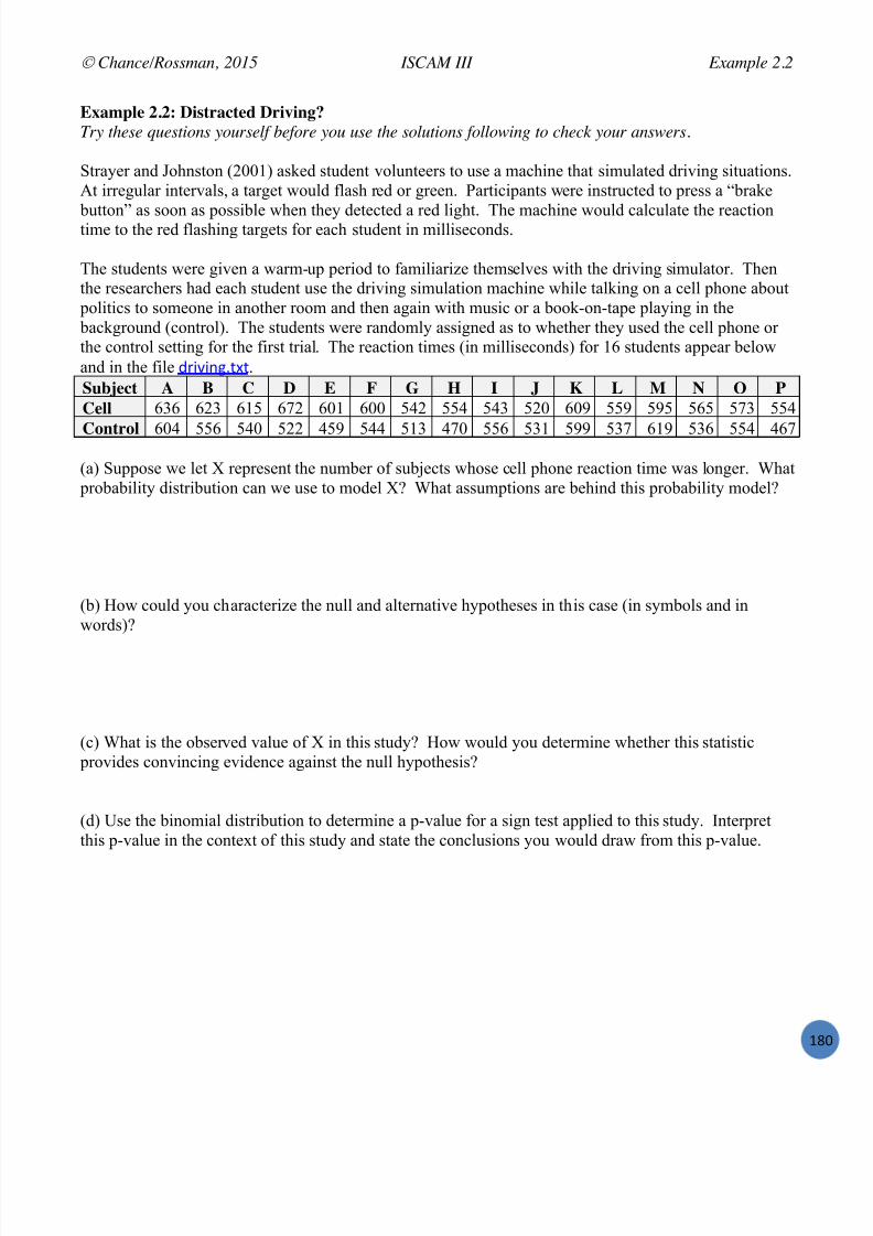
7/25/2019 Text: Investigating Statistical Concepts, Applications, and Methods
http://slidepdf.com/reader/full/text-investigating-statistical-concepts-applications-and-methods 181/428
Chance/Rossman, 2015 ISCAM III Example 2.2
W
Example 2.2: Distracted Driving?Try these questions yourself before you use the solutions following to check your answers.
Strayer and Johnston (2001) asked student volunteers to use a machine that simulated driving situations.At irregular intervals, a target would flash red or green. Participants w ere instructed to press a “brake
button” as soon as possible when they detected a red light. The machine would calculate the reactiontime to the red flashing targets for each student in milliseconds.
The students were given a warm-up period to familiarize themselves with the driving simulator. Thenthe researchers had each student use the driving simulation machine while talking on a cell phone about
politics to someone in another room and then again with music or a book-on-tape playing in the background (control). The students were randomly assigned as to whether they used the cell phone orthe control setting for the first trial. The reaction times (in milliseconds) for 16 students appear belowand in the file ;5'4'.3/%B%. Subject A B C D E F G H I J K L M N O PCell 636 623 615 672 601 600 542 554 543 520 609 559 595 565 573 554
Control 604 556 540 522 459 544 513 470 556 531 599 537 619 536 554 467
(a) Suppose we let X represent the number of subjects whose cell phone reaction time was longer. What probability distribution can we use to model X? What assumptions are behind this probability model?
(b) How could you characterize the null and alternative hypotheses in this case (in symbols and inwords)?
(c) What is the observed value of X in this study? How would you determine whether this statistic provides convincing evidence against the null hypothesis?
(d) Use the binomial distribution to determine a p-value for a sign test applied to this study. Interpretthis p-value in the context of this study and state the conclusions you would draw from this p-value.
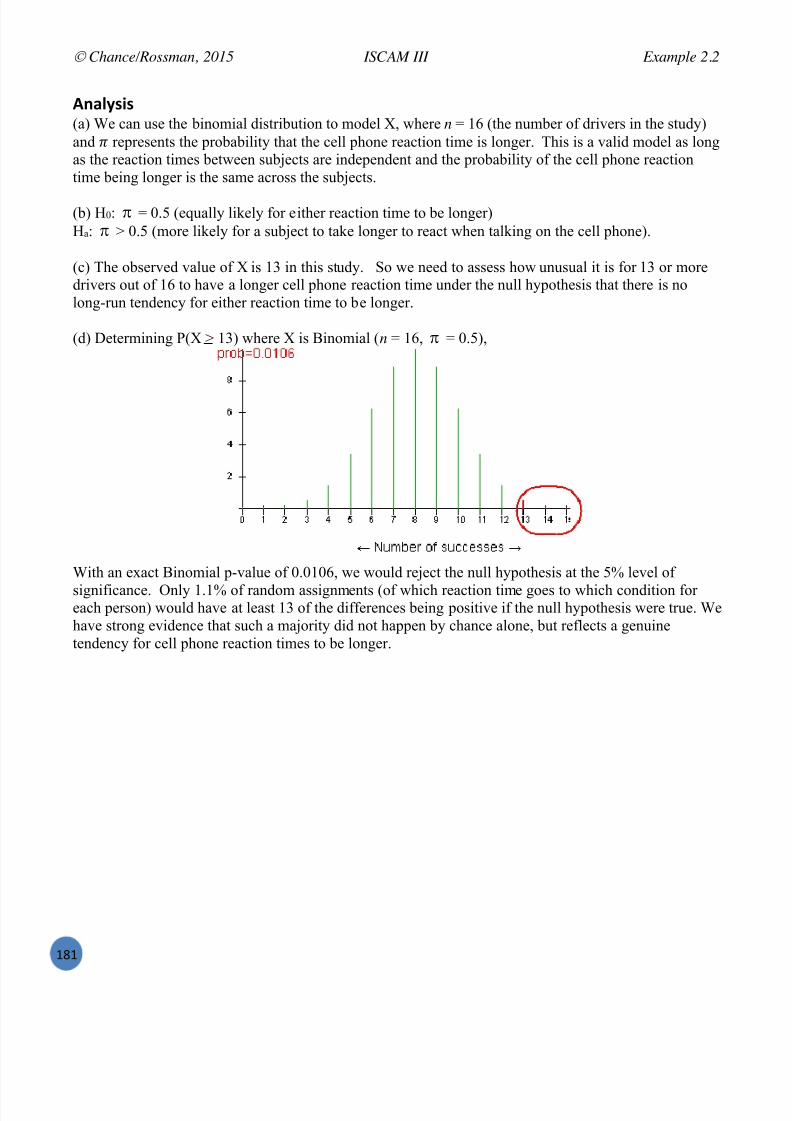
7/25/2019 Text: Investigating Statistical Concepts, Applications, and Methods
http://slidepdf.com/reader/full/text-investigating-statistical-concepts-applications-and-methods 182/428
Chance/Rossman, 2015 ISCAM III Example 2.2
WUW
<*"$6,8,(a) We can use the binomial distribution to model X, where n = 16 (the number of drivers in the study)and represents the probability that the cell phone reaction time is longer. This is a valid model as longas the reaction times between subjects are independent and the probability of the cell phone reactiontime being longer is the same across the subjects.
(b) H 0: = 0.5 (equally likely for either reaction time to be longer)Ha: > 0.5 (more likely for a subject to take longer to react when talking on the cell phone).
(c) The observed value of X is 13 in this study. So we need to assess how unusual it is for 13 or moredrivers out of 16 to have a longer cell phone reaction time under the null hypothesis that there is nolong-run tendency for either reaction time to be longer.
(d) Determining P(X > 13) where X is Binomial ( n = 16, = 0.5),
With an exact Binomial p-value of 0.0106, we would reject the null hypothesis at the 5% level ofsignificance. Only 1.1% of random assignments (of which reaction time goes to which condition foreach person) would have at least 13 of the differences being positive if the null hypothesis were true. Wehave strong evidence that such a majority did not happen by chance alone, but reflects a genuinetendency for cell phone reaction times to be longer.

7/25/2019 Text: Investigating Statistical Concepts, Applications, and Methods
http://slidepdf.com/reader/full/text-investigating-statistical-concepts-applications-and-methods 183/428
Chance/Rossman, 2015 ISCAM III Chapter 2 Summary
W
).<9!/@ R 01BB<@_
In this chapter, you focused on distributions of quantitative data, following up earlier discussion inInvestigation A. In exploring quantitative data, we start with a graph displaying the distribution, such asa dotplot or a histogram. The most relevant features include shape, center, and variability, as well as
deviations from the overall pattern. The appropriate numerical summaries of center include the meanand median, but keep in mind that the median is more resistant than the mean to outliers and skewness.The appropriate numerical summaries of variability include interquartile range (IQR) and standarddeviation, with the IQR also more resistant to outliers and skewness. Remember when examining thevariability of a data set, you are interested in the spread of the values that the variable takes (along thehorizontal axis). In summarizing data, the five-number summary can be very descriptive and you werealso introduced to boxplots, a graphical display of the five-number summary.
After examining the sample distribution, it may be appropriate to ask whether a sample statistic differssignificantly from some claim about the population. For example, whether the sample mean far enoughfrom a conjectured population mean to convince you that the discrepancy did not arise “by chance
alone .” You explored some simulation models, mostly to convince you that the t-distribution provides avery convenient approximation to the sampling distribution of the standardized statistic of a samplemean. This allowed us to approximate p-values and calculate confidence intervals. Keep in mind thatthe logic of statistical significance hasn’t changed – we assume the null hypothesis is true and determinehow often we would get a sample statistic at least as extreme as what was observed. You saw that thislikelihood is strongly affected by not only the sample size but also how much variability is inherent inthe data. You also learned about prediction intervals, as opposed to confidence intervals, for estimatingindividual values rather than the population mean.
These t procedures do come with some validity conditions and should be applied with extreme cautionwith small sample sizes or extreme skewness in the distribution. In this case, you could consider
transforming the variable to rescale the observations to a known probability distribution such as thenormal distribution. You can also apply the sign test which looks at the sign of the values rather than thenumerical outcome and allows you to apply the binomial distribution. Other approaches such as
bootstrapping are very flexible in the choice of statistic.
01BB<@_ -L `.<! _-1 .<J/ K/<@3/2 M3 !.M0 ).<9!/@ Numerical and graphical summaries for describing the distribution of a quantitative variable
C Focus on shape, center, and variability of the distribution, and deviations from overall pattern Properties of numerical summaries (resistance) How to describe, measure, and interpret variability of a quantitative variable Identifying and considering potential explanations for outliers Stating hypotheses in terms of a population mean One-sample t -procedures
C When appropriate to apply; Why helpfulC How to interpret resultsC Alternative approaches if not valid (e.g., data transformations)
Factors that affect the significance of the comparison (e.g., sample size, sample variability) Prediction intervals

7/25/2019 Text: Investigating Statistical Concepts, Applications, and Methods
http://slidepdf.com/reader/full/text-investigating-statistical-concepts-applications-and-methods 184/428
Chance/Rossman, 2015 ISCAM III Chapter 2 Summary
WU#
!/).3-K-N_ 01BB<@_ Summarizing data (dotplots, histograms, boxplots, mean, standard deviation, five-number summary) Simulating a sampling distribution from a finite population One-sample t -procedures Transforming data
)='87% '( 9:'7%54:%, (': <*"$6E8*> -*% B%"*
Study design One quantitative variable from large population or processDescriptive [ N1**&.;(
'()&*;1%8-1%+'(%135&* F-&%%'), 8&)>&3,G'()&*=1B8-1%or =1B8-1%'()&*(2**&56AA8-1%
C'.'%&= N1**&.;(b5&8+ a E1%8-1%b5&8+ a j'(%135&*b5&8+ a M1B8-1%$%&% a M&(') $%&%'(%')( a E'(8-&6 E,()5'8%'4, $%&%'b5&8+ a O51=&='-'%6 O-1%
Parameter = population mean or process mean (or use sign test or bootstrapping) Null Hypothesis H0: = 0 Simulation Random sample from finite population or bootstrappingCan use tprocedures if
Normal population (symmetric sample distribution) or large sample size (e.g.,larger than 30)
Test statistic t 0 = ( x )/( ns / )Confidenceinterval
x + nst n /*1
Predictioninterval
x + *1nt s n/11 (with normally distributed population)
R Commands %/%,(%FB7 &-%,5.&%'4,_`%<1/(';,;`7_X7 )1.9/-,4,- _ X/VRGraw data in “x” '()&*1.,(&*8-,% (2**&56 (%&%'(%')( xbar ( x , sample mean) sd (s, sample standard deviation) n (sample size) hypothesized mean ( 0) alternative (“less”, “greater”, or “two.sided”) Optional: conf.level (s)
Minitab $%&% a M&(') $%&%'(%')( a W:$&*8-, %Input variable column or summary statistics
7/25/2019 Text: Investigating Statistical Concepts, Applications, and Methods
http://slidepdf.com/reader/full/text-investigating-statistical-concepts-applications-and-methods 185/428
Chance/Rossman, 2015 ISCAM III Chapter 3
WUP
CHAPTER 3: COMPARING TWO PROPORTIONS
In this chapter, you will focus on comparing results from two groups on a categorical variable. Thesegroups could be samples from different populations or they could have been deliberately formed duringthe design of the study (a third source of possible randomness). You will again consider multiple ways
to analyze the statistical significance of the difference in the groups, namely simulation, exact methods,and normal approximations to answer whether the observed difference in the groups could havehappened “by chance alone.” You will also continue to consider issues of statistical confidence andtypes of errors. A key consideration to keep in mind will be the scope of conclusions that you can drawfrom the study based on how the data were collected.
Section 1: Comparing two population proportionsInvestigation 3.1: Teen hearing loss (cont.) – Tables, conditional props, bar graphs, z-proceduresInvestigation 3.2: Nightlights and near-sightedness – Association, confounding
Section 2: Types of Studies
Investigation 3.3: Handwriting and SAT scores – Observational studies, experimentsInvestigation 3.4: Have a nice trip – Random assignment, scope of conclusionsInvestigation 3.5: Botox for back pain – Designing experiments
Section 3: Comparing two treatment probabilitiesInvestigation 3.6: Dolphin therapy – Randomization testInvestigation 3.7: Is yawning contagious? – Fisher’s exact t estInvestigation 3.8: CPR vs. chest compressions – z-procedures
Section 4: Other StatisticsInvestigation 3.9: Flu vaccine – Relative riskInvestigation 3.10: Smoking and lung cancer – Types of observational studies, odds ratioInvestigation 3.11: Sleepy drivers – Application
Example 3.1: Wording of QuestionsExample 3.2: Worries about Terrorist Attacks
WUP
" # $ % & ' ( ) & ' " (
+ & ) & ' % & ' , ) -
. / " , $ 0 & %
2 0 0
- ' , ) & ' / " % ) "
3 4 $ & 5 / 3 %

7/25/2019 Text: Investigating Statistical Concepts, Applications, and Methods
http://slidepdf.com/reader/full/text-investigating-statistical-concepts-applications-and-methods 186/428

7/25/2019 Text: Investigating Statistical Concepts, Applications, and Methods
http://slidepdf.com/reader/full/text-investigating-statistical-concepts-applications-and-methods 187/428
Chance/Rossman, 2015 ISCAM III Investigation 3.1
W
Definition: The simplest statistic for comparing a binary variable between two groups is thedifference in the proportion of “successes” for each group. These proportions, calculated separatelyfor each group rather than looking at the overall proportion, are called conditional proportions . In this case, we compute the difference in the proportion of teens with some level of hearing loss
between the two years ( 94ˆ
p = 480/2928 06ˆ
p = 333/1771).
The next step is to examine an effective graphical summary for comparing the two groups.
!%7=*'$'>6 2%+'4: – 0%>;%*+%5 C": N:"?=,
M* @ Create (and view) a matrix in R to store the counts from the two-way table
. 6;B3?<D ! 0B73?[&I&]a-Q #]]aQ (((Q ,](a*Q <3C>!#Qm A?0<B0;9 ! 4?97&I&59C0; 4C995Q 5<C 4C995*Q I&5b]5Q 5-^5***. 6;B3?<D
Convert to a matrix of conditional proportions (margin =1 for row proportions, margin = 2 for
column proportions) . 6;B3?<D83C8 ! 83C8=7BL4;&6;B3?<DQ 0B3D?<!#*. 6;B3?<D83C8
Create a segmented bar graph. LB384C7&6;B3?<D83C8Q 4;D;<A!UQ 14BL!583C8C37?C<5*
M* B8*8+"# Enter the two-way table into the Minitab worksheet. Use
column names and row labels. Choose Graph > Bar Chart . Use the pull-down menu to indicate that the Bars represent
Values from a table. Select the Two-way table / Stack option and press OK . Enter the columns with the two-way table into the Graph
variables box (here C2 and C3). Enter the row labels into the Row labels box (here C1). Press Chart Options and select Show Y as Percent and
Within categories at level 1 . Press OK twice.
(f) Use technology to create numerical and graphical summaries for these summarized data. Write asentence or two comparing the distributions of hearing loss between these two studies. Be sure to report
an appropriate statistic.
(g) Is it possible that the two sample proportions (with some hearing loss) might have differed by thismuch even if the overall population proportion was the same for both years?

7/25/2019 Text: Investigating Statistical Concepts, Applications, and Methods
http://slidepdf.com/reader/full/text-investigating-statistical-concepts-applications-and-methods 188/428
Chance/Rossman, 2015 ISCAM III Investigation 3.1
WUT
M*(%:%*+8"$ 0+"+8,+87, The previous question should look very familiar. As we’ ve said before, it certainly is possible to obtainsample proportions this far apart, just by random chance, even if the population proportions (of teenswith some hearing loss) were the same. The question now is to ask how likely such a difference would
be if the population proportions were the same. We can answer this question by modeling the sampling
variability, arising from taking random samples from these populations, for the difference in two sample proportions. Investigating this sampling variability will help us to assess whether this particulardifference in sample proportions is strong evidence that the population proportions actually differ.
(h) Let 94 represent the proportion of all American teenagers in 1994 with at least some hearing loss,and similarly for 06. Define the parameter of interest to be 94 – 06, the difference in the population
proportions between these two years. State appropriate null and alternative hypotheses about this parameter to reflect the researchers’ conjecture that hearing loss by teens is becoming more prevalent.
Ho:
Ha:
(i) Explain in your own words what we want the p-value to measure in this case.
08;4$"+8'*(j) As before, we will begin our inferential analysis by assuming the null hypothesis is true. What“random process” are we simulating? What is the source of the randomness in this study? What do weneed to assume to perform this simulation?
(k) So under the null hypothesis we really only have one value of to estimate – the common population proportion with hearing loss for these two years. What is your best estimate for from thesample data? [ Hint : Think about combining the two years together.]
(l) Describe how you could carry out a simulation analysis to investigate whether the observeddifference in sample proportions provides strong evidence that the population proportions with hearingloss differed between these two time periods. [ Hint : Think about replicating the randomness in thestudy but in a world where the null hypothesis is true.]

7/25/2019 Text: Investigating Statistical Concepts, Applications, and Methods
http://slidepdf.com/reader/full/text-investigating-statistical-concepts-applications-and-methods 189/428
Chance/Rossman, 2015 ISCAM III Investigation 3.1
W
We will begin our simulation analysis by assuming the population proportion is actually this value ( =(480+333)/(2928+177) = 0.173). We simulate the drawing of two different random samples from this
population, one to represent the 1994 study and the other for the 2006 study. Because the population isvery large compared to the sample sizes, we will model this by treating the population as infinite andsampling from a binomial process. Then we examine the distribution of the difference in the conditional
proportions with some hearing loss between these two years. Finally, we repeat this random sampling process for many trials. [Note: We can assume = 0.173 without loss of generality, but you might wantto verify this with other values for as well.]
(m) Follow the commands below to randomly sample one “could have been” difference in conditional proportions under the null hypothesis :
1. Simulate taking one random sample of 2928 teenagers (representing the 1994 study) from a population in which = 0.173 have at least some hearing loss and count the number of successes(with hearing loss in the sample):
( _ !V!U7 )1**1. _ X/WT# M* @
. IC2<7,bb] ! 3L?<C0&,Q 9?d; ! #b#aQ 83CL!=,c(*
. IC2<7,bb] E'(8-&6( %+, 5,(2-%( M* B8*8+"#
Choose Calc > Random Data > Binomial Specify 1 row to generate, Store in column nIC2<7,bb]n , Number of trials = 2928,and Event probability = 0.173 (You need the single quotation marks around the columnname to refer to it directly.)
2. Now simulate (and view) taking a random sample of 1771 teenagers (for the 2006 study) from a population also with = 0.173 and count the number of successes in this sample.
Technology: Repeat the above steps but change the sample size and column/vector name.
3. Calculate (by hand) the difference in the conditional proportions with hearing loss for these two“could have been” samples. [ Hint: How do you do this based on the randomly generated “numbe r ofsuccesses” in each sample?]
(n) Will everyone in the class get the same answers to (m)? Explain.
(o) How does the difference in sample proportions you just generated at random, assuming that the twoyears have the same population proportion, compare to the observed difference in sample proportions inthe actual studies from (e)?
SIMILAR FURTHER FROM ZERO CLOSER TO ZERO
But to evaluate how unusual such a result is when the null hypothesis is true, we want to generate manymore outcomes assuming the null hypothesis to be true.

7/25/2019 Text: Investigating Statistical Concepts, Applications, and Methods
http://slidepdf.com/reader/full/text-investigating-statistical-concepts-applications-and-methods 190/428
Chance/Rossman, 2015 ISCAM III Investigation 3.1
WUV
(p) To create the null distribution of the differences in sample proportions, you will generate 1000random samples from each population and calculate the difference in conditional proportions each time,storing the results in 2 different vectors/columns:]2*=,5 19 5&.;1* (&*8-,( _ WXXX
M* @
. 86B7b] ! 3L?<C0&,---Q #b#aQ =,c(*$#b#a E'4';,( .2*=,5 19 (2)),((,( =6 (
. 86B7-^ ! 3L?<C0&,---Q ,cc,Q =,c(*$,cc, %1 3,% (&*8-, 851815%'1.( F^Y( G/
. 86B7A?GG9 ! 86B7b] ) 86B7-^ D12 .1< +&4, WXXX ;'99,5,.),(/ M* B8*8+"#
Choose Calc > Random Data > Binomial , generate 1000 rows of data and store innIC2<7,bb]n with Number of trials 2928 and Event probability .173.Choose Calc > Calculator , store the result in 83C8,bb] , with expression nIC2<7,bb]n$#b#a(NUe. 4;7 I# ! I,$#b#a ) Repeat for 2006 data but change the sample size, and store the counts in nIC2<7#--^n and thesample proportions in 83C8#--^ .Choose Calc > Calculator , store the result in A?GG, expression: n83C8,bb]n)n83C8#--^n You now have 1000 differences in p
ˆ
’s . (NUe. 4;7 I_ ! I# – I] )
(q) Display a histogram and summary statistics of the null distribution of differences in sample proportions:
M* @ . 8B3&0G3C>!I&(Q,** N5,&%,( # 51<( '. 35&8+ <'.;1< . 6?97&86B7b]*O 6?97&86B7-^* Z(, & (,*')1-1. %1 (,8&5&%, )1**&.;( . 6?97&86B7A?GG9Q 4BL;49!U* @. [$%2;'17 )&. .!!4 %+, 35&8+ <'.;1< . 0;B<&86B7b]*O 0;B<&86B7-^*. 0;B<&86B7A?GG9*. 9A&86B7b]*O 9A&86B7-^*. 9A&86B7A?GG9*
M* B8*8+"#Choose Graph > Histogram > Simple, OK. Specify n83C8,bb]n n83C8#--^n nA?GGn (double click on each in the left panel) in the Graph variables box. Press OK.Choose Stat > Basic Statistics > Display Descriptive Statistics and specify the threecolumns in the Variables box, press OK.
Describe the null distribution of the difference in sample proportions. Does it behave as you expected?In particular, does the mean of this distribution make sense? (How does it compare to the means of theindividual p
ˆ
distributions?) Explain.
(r) Now determine the empirical p-value by counting how often the simulated difference in conditional proportions is at least as extreme as the actual value observed in the study:

7/25/2019 Text: Investigating Statistical Concepts, Applications, and Methods
http://slidepdf.com/reader/full/text-investigating-statistical-concepts-applications-and-methods 191/428
Chance/Rossman, 2015 ISCAM III Investigation 3.1
W
I+,(, )1**&.;( )12.% +1< *&.6 ('*2-&%,; ;'99,5,.),( &5, =,-1< %+, 1=(,54,; (%&%'(%')F X/X!PG =6 )5,&%'.3 & M11-,&. 4&5'&=-, FW <+,. %+, (%&%,*,.% '( %52,7 X 1%+,5<'(,G7 (2**'.3%+, 1.,(7 &.; %+,. ;'4';'.3 =6 %+, .2*=,5 19 (&*8-,( '. %+, ('*2-&%'1./
M* @. 8HB42;!920&86B7A?GG9 j! )=-#]*$,---
. 8HB42; M* B8*8+"#
Choose Calc > Calculator , store result in 8HB42; ,expression : 920&A?GG j! )=-#]* $,---(NUe. 4;7 @,!920&nA?GGn j! )=-#]*$,---NUe. 83?<7 @, )
Report your empirical p-value and indicate what conclusion you would draw from it.
B"+=%;"+87"$ B'5%$(s) It turns out that there is no “exact” method for calculating the p -value here, because the difference intwo binomial variables does not have a binomial, or any other known, probability distribution.However, did the histogram you examined remind you of any other probability distribution?
(t) Overlay a normal curve on your null distribution and/or examine a normal probability plot to evaluatewhether the simulated differences appear to “line up” with observations from a standard normaldistribution.
M* @. ?9IB0BAA<C30&86B7A?GG9*. \\<C30&86B7A?GG9*
M* B8*8+"#Right click on the graph and choose Add > Distribution Fit. Because the default distribution is
Normal, press OK.Choose Graph > Probability Plot , Single , press OK , specify the column of simulateddifferences in the Graph variables box, and press OK.
Does the normal model appear to be a reasonable approximation to the null distribution?
9:'#"#8$8+6 2%+'4: There is a theoretical result that the difference in two normal distributions will also follow a normaldistribution. When our sample sizes ( n1 and n2) are large, we know the individual binomial distributionsare well approximated by normal distributions. Consequently, the difference of the sample proportions

7/25/2019 Text: Investigating Statistical Concepts, Applications, and Methods
http://slidepdf.com/reader/full/text-investigating-statistical-concepts-applications-and-methods 192/428
Chance/Rossman, 2015 ISCAM III Investigation 3.1
WVW
will be well approximated by a normal distribution as well. The mean of this distribution is simply thedifference in the means of the individual normal distributions.
(u) How does the variability (SD) of the difference in pˆ values compare to the variability of the
individual pˆ
distributions? Explain why this makes intuitive sense.
SIMILAR LARGER SMALLER
Explanation:
Central Limit Theorem for the difference in two sample proportionsWhen taking two independent samples (of sizes n1 and n2) from large populations, the distribution of thedifference in the sample proportions ( 21
ˆˆ
p p ) is approximately normal with mean equal to 1 – 2 and
standard deviation equal to SD( 21
ˆˆ
p p ) =2
22
1
11 )1()1(
nn
.
Under the null hypothesis H 0: 1 2 = 0, the standard deviation simplifies to
21
11)1(
nn
where is the common population proportion.
Technical Conditions: We will consider the normal model appropriate if the sample sizes are large,namely n1 1 > 5, n1(1 1) > 5, n2 2 > 5, n2(1 2) > 5, and the populations are large compared to thesample sizes.
Note: The variability in the differences in sample proportions is larger than the variability of individualsample proportions. In fact, the variances (standard deviation squared) add, and then we take the squareroot of the sum of variances to find the standard deviation.
However, to calculate these values we would need to know 1, 2, or . So again we estimate thestandard deviation of our statistic using the sample data.
Case 1: When the null hypothesis is true, we are assuming the samples come from the same population,so we “ pool” the two samples together to estimate the common population proportion of successes.That is, we estimate by looking at the ratio of the total number of successes to the total sample size:
21
21ˆ
nn
X X p =
sizesampletotal
successesof numbertotal
nn
pn pn
21
2211
ˆˆ
Then use we use this value to calculate the standard error of 21
ˆˆ
p p to be:
2121
11)
ˆ
1(ˆ
)ˆˆ
(nn
p p p pSE

7/25/2019 Text: Investigating Statistical Concepts, Applications, and Methods
http://slidepdf.com/reader/full/text-investigating-statistical-concepts-applications-and-methods 193/428
Chance/Rossman, 2015 ISCAM III Investigation 3.1
W
(v) Use these theoretical results to suggest the general formula for a test statistic and a method forcalculating a p-value to test H 0: 1 2 = 0 (also expressed as H 0: ) versus the alternativeHa: 1 2 < 0. (This is referred to as the two-sample z-test or two proportion z-test .)
Test statistic = z = −
=
(w) Calculate and interpret the value of the test statistic specified in (v) as applied to the hearing lossstudy.
94ˆ
p 06ˆ
p = pˆ
=
SE( 94
ˆ
p 06
ˆ
p )=
test statistic: z =
interpretation:
(x) Is the standard error close to the empirical standard deviation from your simulation results?
(y) Compute the p-value for this test statistic and compare it to your simulation results.
)'*(85%*7% M*+%:F"$Case 2: When we make no assumptions about the populations (for example, when we are not testing a
particular null hypothesis but only estimating the parameter), we will use a different formula toapproximate the standard deviation of 21
ˆˆ
p p .
(z) Using the above CLT result, suggest a general formula for a confidence interval for the difference in population proportions 1 – 2.
(aa) Calculate and interpret a 95% confidence interval to compare hearing loss of American teenagers inthese two years. Is this confidence interval consistent with your test of significance? Explain.

7/25/2019 Text: Investigating Statistical Concepts, Applications, and Methods
http://slidepdf.com/reader/full/text-investigating-statistical-concepts-applications-and-methods 194/428
Chance/Rossman, 2015 ISCAM III Investigation 3.1
WV#
Note: It is technically incorrect to say there has been a 0.1% to 4.7% increase, because “percentagechange” implies a multiplication of values, not an addition or subtraction as we are considering here. Itwould be acceptable to say that the increase is between 0.1 and 4.7 percentage points .
!%7=*87"$ )'*58+8'*,
The above Central Limit Theorem holds when the populations are much larger than the samples (e.g.,more than 20 times the sample size) and when the sample size is large. We will consider the lattercondition met when we have at least 5 successes and at least 5 failures in each sample (so there are fournumbers to check).
Note: A “Wilson adjustment” can be used with this confidence interval as before, this time putting oneadditional success and one additional failure in each sample. This adjustment will be most useful whenthe proportions are close to 0 or 1 (that is when the sample size conditions above are not met).
(bb) Summarize your conclusions from this study. Be sure to address statistical significance, statisticalconfidence, and the populations you are willing to generalize the results to. Also, are you willing to
conclude that the change in the prevalence of hearing loss is due to the increased use of ear buds amongteenagers between 1994 and 2006? Explain why or why not.
0+456 )'*7$4,8'*, We have moderate evidence against the null hypothesis (p-value 0.02, meaning we would get adifference in sample proportions 1
ˆ
p 2
ˆ
p as small as 0.024 or smaller in about 2% of random samplesfrom two populations with 1 = 2). We are 95% confident that the population proportion with somehearing loss is between 0.001 and 0. 047 higher “now” than ten years ago. We feel comfortabl e drawingthese conclusions about the populations the NHANES samples were selected from as they were randomsamples from each population (and there was no overlap in the populations between these two time
periods). However, there are many things that have changed during this time period, and it would not bereasonable to attribute this increase in hearing loss exclusively to the use of ear buds.
9:"7+87% 9:'#$%; TDH<(a) When we conducted the simulation analysis above, we used the same probability of “success”(having some hearing loss) for both years. Why did we do this?(b) How did we decide what common probability of success to use?(c) Why did we count how many samples of the simulation gave a result of 0.024 or smaller (explainthe 0.024 part and t he “or smaller” part).

7/25/2019 Text: Investigating Statistical Concepts, Applications, and Methods
http://slidepdf.com/reader/full/text-investigating-statistical-concepts-applications-and-methods 195/428
Chance/Rossman, 2015 ISCAM III Investigation 3.1
W
!%7=*'$'>6 2%+'4: – !G'\,";?$% E\?:'7%54:%,
!=%':6\C",%5 M*(%:%*7% "??$%+ Select Two proportions Check the box to paste in 2 columns of data (stacked or
unstacked) and press Use data or specify the samplesizes and either the sample counts or the sample proportions and press Calculate .
For the test, check the box for Test of Significance Keep the hypothesized difference at zero and set thedirection of the alternative, press Calculate .
For the confidence interval, check the box, specify theconfidence level and press Calculate CI
M* @ Use '()&*%<18518K%,(%which takes the following inputs:
C observed1 (either the number of successes or sample proportion for first group), n1 (samplesize for first group, observed2 (count or proportion), and n2
C Optional: hypothesized difference and alternative (“less”, “greater”, or “two.sided”) C Optional: conf.level
For example: a '()&*%<18518K%,(%FPUX7 !V!U7 ###7 WTTW7 X7 &-% _ `-,((`7 )1.9/-,4,-_ VRGfinds the p-value for a one-sided alternative as well as a 95% confidence interval for .
M* B8*8+"# Choose Stat > Basic Statistics > 2
Proportions . Specify columns of raw data (stacked or
unstacked) or select Summarized data andenter the number of successes (“Events”) ineach sample and the sample size (“Trials”) ofeach sample.
For a test, under Options select the correctAlternative hypothesis and use the Testmethod pull-down menu to select Use thepooled estimate of the proportion
For a confidence interval, under Options setthe confidence level, a two-sided alternative,and Estimate the proportions separately.
Click OK twice.
21

7/25/2019 Text: Investigating Statistical Concepts, Applications, and Methods
http://slidepdf.com/reader/full/text-investigating-statistical-concepts-applications-and-methods 196/428
Chance/Rossman, 2015 ISCAM III Investigation 3.1
WVR
04;;":6 '( ,8;4$"+8'* "*5 !# ?:'7%54:%, (': 7';?":8*> +G' ?'?4$"+8'* ?:'?':+8'*,
Parameter: 1 2 = the difference in the population proportions of success
To test H 0: 1 2 = 0
1. Simulation : Random samples from binomial processes with common
2. Two-sample z-test :
The test statistic z0 =
2
1
1
1)
ˆ
1(ˆ
2ˆ
1ˆ
nn p p
p p where
studyinnumbertotalsuccessesof numbertotal
nn X X
p 21
21ˆ
is well approximated by the standard normal distribution when n1 pˆ > 5, n1(1 p
ˆ ) > 5, n2 pˆ > 5
and n2(1 pˆ ) > 5, where p
ˆ
is the overall proportion of successes in the two groups put together.
Approximate (100 ! C)% Confidence interval for 1 2:
1. Two-sample z-interval :
An approximate (100 ! C )% interval: 2
22
1
1121
)ˆ
1(ˆ
)ˆ
1(ˆ
*ˆˆ
n p p
n p p
z p p
where z* is the 100 ! (1 C )/2 th percentile from the standard normal distribution.This method is considered valid when n1 1
ˆ
p > 5, n1(1 1
ˆ
p ) > 5, n2 2
ˆ
p > 5, and n2(1 2
ˆ
p ) > 5.
2. Or the Wilson adjustment can be made on the sample proportions and sample sizes first.
Note : We can simplify the technical conditions by verifying that you have independent random samplesfrom two processes or large populations (or one random sample classified by a binary variable) and atleast 5 successes and 5 failures in each group.
Technology: To perform the calculations for these two-sample z-procedures you can use the Theory-Based Inference applet ( %<1 851815%'1.() or Minitab ( $%&% a M&(') $%&%'(%')( a ! O51815%'1.() or'()&*%<18518K%,(% in R.
9:"7+87% 9:'#$%; TDHC USA Today reported that newspapers appear to be losing credibility over time (March, 2004). They cited
a nationwide sample of 1,002 adults, 18 years or older, interviewed via telephone (under the direction ofPrinceton Survey Research Associates) during the period May 6-16, 2002. Of the 932 respondents whowere able to rate the daily newspaper they were most familiar with, 591 rated the paper as “largely
believable” (a 3 or a 4 on the scale). When the same question was asked four years earlier (May 7 – 13,1998), 922 said they could rate their daily paper and of those, 618 rated the paper as “largely
believable.”(a) Are the technical conditions met to calculate the two-sample z-interval for these data? Explain.(b) Calculate and interpret a 95% confidence interval from these data.

7/25/2019 Text: Investigating Statistical Concepts, Applications, and Methods
http://slidepdf.com/reader/full/text-investigating-statistical-concepts-applications-and-methods 197/428
Chance/Rossman, 2015 ISCAM III Investigation 3.2
W
Investigation 3.2: Nightlights and Near-sightedness
Myopia, or near-sightedness, typically develops during the childhood years. Recent studies haveexplored whether there is an association between development of myopia and the use of night-lightswith infants. Quinn, Shin, Maguire, and Stone (1999) examined the type of light children aged 2-16
were exposed to. Between January and June 1998, the parents of 479 children who were seen asoutpatients in a university pediatric ophthalmology clinic completed a questionnaire (children who hadalready developed ser ious eye conditions were excluded). One of the questions asked was “Underwhich lighting condition did/does your child sleep at night?” before the age of 2 years. The followingtwo- way table classifies the children’s eye condition and whether or not they slept with some kind oflight (e.g., a night light or full room light) or in darkness.
Some light Darkness TotalNear-sighted 188 18 206Not near-sighted 119 154 273Total 307 172 479
Definition: When we have two variables, we often specify one to be the explanatory variable andthe other to be the response variable . The explanatory variable is the one that we think might beinfluencing or explaining changes in the response variable, the outcomes of interest.
(a) Which variable, lighting condition or eye condition, would you consider the explanatory variable inthis study and which the response variable?
(b) Calculate conditional proportions to measure the difference in the rate of near sightedness between
the children with and without lighted rooms in this sample. (Use appropriate symbols.) Also produce asegmented bar graph to compare the eye condition of the two lighting groups. Comment on what thisgraph reveals about differences in eye condition between these lighting groups. Do you think thisdifference will be statistically significant? Explain.
Discussion: In the previous investigation, the researchers literally took two different random samples
from two different groups of teens. In this study, the data arose from one sample and each child in thesample was classified according to two variables: lighting condition and eye condition . A naturalresearch question h ere might be “Does use of night lights and room lights increase the rate of near-sightedness in children?” In such a situation, we can instead phrase our hypotheses in terms of theassociation between the two variables:
H0: There is no association between lighting condition and eye condition Ha: There is an association between lighting condition and eye condition
We can also state these hypotheses in terms of underlying population probabilities:

7/25/2019 Text: Investigating Statistical Concepts, Applications, and Methods
http://slidepdf.com/reader/full/text-investigating-statistical-concepts-applications-and-methods 198/428
Chance/Rossman, 2015 ISCAM III Investigation 3.2
WVT
H0: light – darkness = 0 vs. H a: light – darkness > 0where i represents the probability of a near-sighted child in population i.
(c) Briefly discuss how you could modify the simulation procedure used in Investigation 3.1 to reflectthe changes in the study design.
It turns out, it will be valid to use the same inferential analysis procedures here as in Investigation 3.1 aslong as the samples (e.g., room light, darkness) can be considered independent of each other. Onecounter example would be if the observational units had been paired in some way (e.g., brothers andsisters). But if we don’t believe the responses of particular children in lit rooms in this study in any wayrelate to the responses of particular children in the dark rooms, we consider the samples independent ,even though they weren’t literally sampled separately, and use the same Central Li mit Theorem tospecify a normal distribution as a model of the sampling distribution of the difference in the two sample
proportions.
(d) Use technology to perform a two-sample z-test to compare the proportion with near sightedness between these two groups. Report the test statistic and p-value. Also report and interpret a 95%confidence interval from these data.
(e) Because the p-value is so small, would you be willing to conclude that the use of lights causes anincrease in the probability of near-sightedness in children? Explain. If not, suggest a possible alternativeexplanation for the significantly higher likelihood of near sightedness for children with lighting in theirrooms.
Discussion: When we find a highly significant difference between two groups, although we canconclude a significant association between the explanatory and response variables, we are not alwayswilling to draw a cause-and-effect conclusion between the two variables. Though many wanted to usethis study as evidence that it was the lighting that caused the higher rate of near-sightedness, for all weknow it could have been children with poorer vision that asked for more light to be used in their rooms.

7/25/2019 Text: Investigating Statistical Concepts, Applications, and Methods
http://slidepdf.com/reader/full/text-investigating-statistical-concepts-applications-and-methods 199/428
Chance/Rossman, 2015 ISCAM III Investigation 3.2
W
Or there could even be a third variable that is related to the first two and could provide the realexplanation for the observed association. Such a variable is a called a confounding variable .
Definition: In some studies, we may consider one variable the explanatory variable that we suspect hasan effect on the response variable. However, in some studies often there may be other confounding
variables that also differ between the explanatory variable groups and have a potential effect on theresponse variable.
Your alternative explanation in (d) probably identified a potential confounding variable. For example,eye condition of the parents may be related to the explanatory variable (parents with poorer sight aremore likely to use room lighting) and to the response variable (children of near-sighted parents are morelikely to be near-sighted themselves). Because this confounding variable changes with the explanatoryvariable, we have no way of separating out the effects of this variable and those of the explanatoryvariable. This prevents us from drawing a cause-and-effect conclusion between lighting condition andeye condition .
One way to visualize confounding is to examine a diagram of the study design. For the night-light andeye condition study we considered lighting the explanatory variable and eye condition the response.Some light
Children Eye condition
No light
Observational units Explanatory variable Response variable
But we are conjecturing the parents’ eye condition mig ht also be changing across the two groups.
Some light Mostly near sightedChildren parents Eye condition
No light Mostly parents withgood eyesight
So when those who had lighting in their room develop near-sightedness, there are two equally plausibleexplanations because two things have changed for that group and we can’t separate them out.
(f ) It has been suggested that “low birth weight” is a po ssible confounding variable in this study. Doesthis seem plausible to you? Describe circumstances under which this would be a confounding variable.

7/25/2019 Text: Investigating Statistical Concepts, Applications, and Methods
http://slidepdf.com/reader/full/text-investigating-statistical-concepts-applications-and-methods 200/428
Chance/Rossman, 2015 ISCAM III Investigation 3.2
WVV
(g) In this study, 70% of the children were Caucasian. Does this mean “race” is a possible confoundi ngvariable? What should you be concerned about? What about the region of the country where the clinicwas located?
Discussion: Keep in mind that the issue of confounding, and whether or not you can draw a cause-and-effect conclusion between explanatory and response variables, is very different from the issue ofgeneralizability. We are willing to generalize to a larger population when the study design involvesrandom sampling of observational units from the population. This is a separate question from how theobservational units were formed into subgroups.
0+456 )'*7$4,8'*,
With a very small p-value, we have extremely strong evidence that the relationship we observed in thesample data (use of light in the child’s room is associated with higher ra tes of myopia) did not occur bychance alone. There appears to be a genuine connection here, more than luck of the draw, but we can’tnecessarily draw a causal relationship between lighting and eyesight from this study. We should also becautious in generalizing these results too far beyond the type of families that visit this clinic in this partof the United States.

7/25/2019 Text: Investigating Statistical Concepts, Applications, and Methods
http://slidepdf.com/reader/full/text-investigating-statistical-concepts-applications-and-methods 201/428

7/25/2019 Text: Investigating Statistical Concepts, Applications, and Methods
http://slidepdf.com/reader/full/text-investigating-statistical-concepts-applications-and-methods 202/428
Chance/Rossman, 2015 ISCAM III Investigation 3.3
!XW
SECTION 2: TYPES OF STUDIES
In the previous investigation, we cautioned against jumping to a cause-and-effect conclusion when astatistically significant association is found between the response and explanatory variables. But whencan we potentially draw such a conclusion?
Investigation 3.3: Handwriting and SAT Scores
An article about handwriting appeared in the October 11, 2006 issue of the Washington Post . Thearticle mentioned that among students who took the essay portion of the SAT exam in 2005-06, thosewho wrote in cursive style scored significantly higher on the essay, on average, than students who used
printed block letters. Researchers wanted to know whether simply writing in cursive would be a way toincrease scores.
(a) Identify the explanatory and response variables in this study. Also classify the variables asquantitative or categorical.
Explanatory:
Response:
(b) Would you conclude from this study that using cursive style causes students to score better on theessay? If so, explain why. If not, identify a potential confounding variable, and explain how it providesan alternative explanation for why the cursive writing group would have a significantly higher averageessay score.
The article also mentioned a different study in which the same one essay was given to all graders. Butsome graders were shown a cursive version of the essay and the other graders were shown a version with
printed block letters. Researchers randomly decided which version the grader would receive. Theaverage score assigned to the essay with the cursive style was significantly higher than the average scoreassigned to the essay with the printed block letters.
(c) Explain a key difference between how this study was conducted and how the first study wasconducted.
(d) Would the difference cited in (c) make you more willing to draw a cause-and-effect conclusion between writing style and SAT score with the second study than with the first one? Explain.

7/25/2019 Text: Investigating Statistical Concepts, Applications, and Methods
http://slidepdf.com/reader/full/text-investigating-statistical-concepts-applications-and-methods 203/428
Chance/Rossman, 2015 ISCAM III Investigation 3.3
!X
Definition: An observational study is one in which the researchers passively observe and recordinformation about the observational units. In an experimental study , the researchers actively impose theexplanatory variable (often called treatment ) on the observational units (can also be called theexperimental units in an experiment).
(e) Classify the first and second study above as observational or experimental:
Study of 2006 exams:
Study of one response written both ways:
(f) Explain why the experimental study should be less susceptible to the potential for a confoundingvariables between the writing style and the score.
(g) Discuss one disadvantage to the experimental study compared to the observational study for thisresearch question.
0+456 )'*7$4,8'*, The second study determined for each judge whether they would grade the exam written in block letters
or in cursive letters. Because it was the same exam otherwise, there shouldn’ t be any other reason for thedifference in scores apart from the type of writing. For this reason, because the difference was
statistically significant, we will be willing to conclude that the writing style caused the difference inscores. However, this only tells us about that one exam and in the slightly artificial condition of askingthe judges to grade the exam. We don’t know whether the same effect would be found on other essays orconditions. By looking at the 2006 exams, we know that actual student papers were graded by actual
judges, a more realistic setting, but also with the potential for confounding variables between the writingstyle and grade, such as student preparation prior to the exam.
9:"7+87% 9:'#$%; TDTIn a study published in the July 2003 issue of the journal Psychosomatic Medicine , researchers reportedthat people who tend to think positive thoughts catch a cold less often than those who tend to thinknegative thoughts. The scientists recruited 334 initially healthy male and female volunteers aged 18 to54 years through advertisements in the Pittsburgh area, and they first interviewed them over a two week
period to gauge their emotional state, eventually assigning them a numerical score for positive emotionsand a numerical score for negative emotions. Then the subjects were quarantined before the researchersinjected rhinovirus, the germ that causes colds, into each subject’s nose. The subjects were thenmonitored for five days for the development of cold-like symptoms. Subjects scoring in the bottomthird for positive emotions were three times more likely to catch a cold than those scoring the top thirdfor positive emotions. According to the above definitions, is this an observational study or a randomizedexperiment? Would it be valid to draw a cause and effect conclusion from their results? Explain.

7/25/2019 Text: Investigating Statistical Concepts, Applications, and Methods
http://slidepdf.com/reader/full/text-investigating-statistical-concepts-applications-and-methods 204/428
Chance/Rossman, 2015 ISCAM III Investigation 3.4
!X#
Investigation 3.4: Have a Nice Trip
An area of research in biomechanics and gerontology concerns falls and fall-related injuries, especiallyfor elderly people. Recent studies have focused on how individuals respond to large posturaldisturbances (e.g., tripping, induced slips). One question is whether subjects can be instructed to
improve their recovery from such perturbations. Suppose researchers want to compare two suchrecovery strategies, lowering (making the next step shorter, but in normal step time) and elevating (usinga longer or normal step length with normal step time). Subjects will have first been trained on one ofthese two recovery strategies, and they will be asked to apply it after they feel themselves tripping. Theresearchers will then induce the subject to trip while walking (but harnessed for safety), using aconcealed mechanical obstacle.
Suppose the following 24 subjects have agreed to participate in such a study. Both males and femalewere recruited because females tend to have better balance (lower center of gravity).
Females: Alisha, Alice, Betty, Martha, Audrey, Mary, Barbie, Anna
Males: Matt, Peter, Shawn, Brad, Michael, Kyle, Russ, Patrick, Bob, Kevin, Mitch, Marvin,Paul, Pedro, Roger, Sam
(a) One way to design an experiment for this study would be to assign the eight females to use theelevating strategy and the 16 males to use the lowering strategy. Would this be a reasonable strategy? Ifnot, identify a better method for deciding who uses which strategy.
Definition: In a well-designed experiment, experimental units are randomly assigned to the treatmentgroups. Each unit is equally likely to be assigned to any of the treatments.
(b) Let’s explore this random assignment process to determine whether it does “work.” First, let’s focuson the sex variable. Suppose we put each person’s name on a slip, put those slips in a hat and mix themup thoroughly, and then randomly draw out 12 slips for names of people to assign to the elevatingstrategy. What proportion of this group do you expect will be male? What proportion of the loweringstrategy do you expect will be male? Do you think we will always get a 8/8 split of the male subjects (8males in each treatment group)?

7/25/2019 Text: Investigating Statistical Concepts, Applications, and Methods
http://slidepdf.com/reader/full/text-investigating-statistical-concepts-applications-and-methods 205/428
Chance/Rossman, 2015 ISCAM III Investigation 3.4
!X
(c) To repeat this random assignment a largenumber of times to observe the long-run behavior,we will use the Randomizing Subjects applet.Open the applet, and press the Randomize button.
What proportion of subjects assigned to Group 1 are men? Of Group 2? What is the difference in thesetwo proportions?
You will notice that the difference in the proportion male is shown in the dotplot in the bottom graph. Inthis graph, the observational unit is one repetition of the random assignment, and the variable is thedifference in proportions of men between the two groups.
(d) Press the Randomize button again. Was the difference in proportions of men the same this time?
(e) Change the number of replications from 1 to 198 (for 200 total, and press the Randomize button.The dotplot will display the difference between the two proportions of men for each of the 200repetitions of the random assignment process. Where are these values roughly centered?
(f) Click on the most extreme dot (positive or negative). The graph should update to show thegroups. What difference in proportion male did you find here? Did you ever get an absolutedifference as large as 0.6667 (a 12/4 split)? Which is more likely, ending up with a 12/4 split inmales or ended up with an 8/8 split in males?
(f) Does random assignment always equally distribute/balance the men and women between the twogroups?
(g) Is there a tendency for there to be a similar proportion of men in the two groups? How are youdeciding? What does this tell you about the plausibility of any later difference in the two groups beingattributed to females having better balance?
Discussion: A 12/4 split in males would be problematic, because then if the treatment group thathad all males s howed worse balance, we wouldn’t know whether it was because of the strategy theyuse or because they were all males and the other group was more likely to recover their balance
because they had mostly females. But with random assignment, such an unequal split is unlikely.Instead, the random assignment usually creates an 8/8 split or a 9/7 split. In this case, the groupsare balanced on the sex variable and sex is no longer confounded with recovery.
7/25/2019 Text: Investigating Statistical Concepts, Applications, and Methods
http://slidepdf.com/reader/full/text-investigating-statistical-concepts-applications-and-methods 206/428
Chance/Rossman, 2015 ISCAM III Investigation 3.4
!XR
(h) Prior research has also shown that the likelihood of falling is related to variables such aswalking speed, stride rate, and height, so we would like the random assignment to distribute thesevariables equally between the groups as well. In the applet, use the pull-down menu to switch fromthe sex variable to the height variable. The dotplot now displays the differences in average height
between Group 1 and Group 2 for these 200 repetitions. In the long-run, does random assignment
tend to equally distribute the height variable between the two groups? Explain.
(i) Suppose there is a “balance gene” that is related to people’s ability to recover from a trip. We didn’tknow about this gene ahead of time, but if you select the “R eveal gene? ” button and then select “gene”from the pull-down menu, the applet shows you this gene information for each subject and also how the
proportions with the gene differ in the two groups. Does this variable tend to equalize between the twogroups in the long run? Explain.
(j) Suppose there were other “ x-variables” th at we could not measure such as stride rate or walkingspeed. Select the “R eveal both? ” button and use pull -down menu to display the results for the x-variable(B:4&5). Does random assignment generally succeed in equalizing this variable between the two groupsor is there a tendency for one group to always have higher results for the x-variable? Explain.
Discussion : The primary goal of random assignment is to create groups that equalize any potential
confounding variables between the groups, creating explanatory variable groups that overall differ onlyon the explanatory variable imposed. Note that this “balancing out” applies equally well to variablesthat can be observed (such as sex and height) and variables that may not have been recorded (such asage or walking speed) or that cannot be observed (such as a hidden gene). Although we could haveforced variables like sex and height to be equally distributed between the two groups, the virtue ofrandom assignment is that it also tends to balance out variables that we might not have thought of aheadof time and variables that we might not be able to see or control. Thus, when we observe a “ statisticallysignificant” difference in the response variable between the two groups at the end of the study, w e feelmore comfortable attributing this difference to the explanatory variable (e.g., recovery strategyemployed), because that should have been the only difference between the groups.
(k ) Suppose the “tripping” study finds a statistically significant difference between the two strategies.What conclusion would you draw? For what population? What additional information would you needto know?

7/25/2019 Text: Investigating Statistical Concepts, Applications, and Methods
http://slidepdf.com/reader/full/text-investigating-statistical-concepts-applications-and-methods 207/428
Chance/Rossman, 2015 ISCAM III Investigation 3.4
!X
Keep in mind that cause-and-effect conclusions are a separate consideration from the generalizabilityof the results to a larger population. From now on we will consider each of these issues in our finalconclusion as shown in the table below (adapted from Ramsey and Schafer’s The Statistical Sleuth ):
Splitting units into groups
By random assignment No randomassignment
Selectionunits frompopulation
Randomsampling
A random sample isselected from one
population; units arethen randomly assignedto different treatmentgroups(e.g., survey incentives)
Random samplesare selected fromexisting distinct
populations(e.g., teen hearingloss)
Inferencescan be
generalizedto
populations
Not
randomsampling
A groups of study units
is found; units are thenrandomly assigned totreatment groups(e.g., tripping study)
Collections of
available unitsfrom distinctgroups areexamined(e.g., nightlights)
Potential forsamplingbias
Can draw cause andeffect conclusions
May beconfounding
variables
9:"7+87% 9:'#$%; TDU A team of researchers (Singer, et al., 2000) used the Survey of Consumer Attitudes to investigatewhether incentives would improve the response rates on telephone surveys. A national sample of 735households was randomly selected, and all 735 of the households were sent an “advance letter”explaining that the household would be contacted shortly for a telephone survey. However, 368households were randomly assigned to receive a monetary incentive along with the advance letter, andthe other 367 households were assigned to receive only the advance letter.(a) Identify the explanatory and response variables.(b) Is this an observational study or an experiment? Explain how you are deciding.(c) If these researchers find a statistically significant difference in the response rate between these twogroups, would it be reasonable to draw a cause-and-effect conclusion? Explain (including any additional
information you would need to know to decide).(d) To what population is it reasonable to generalize these results? Explain (including any additionalinformation you would need to know to decide).

7/25/2019 Text: Investigating Statistical Concepts, Applications, and Methods
http://slidepdf.com/reader/full/text-investigating-statistical-concepts-applications-and-methods 208/428
Chance/Rossman, 2015 ISCAM III Investigation 3.5
!XT
Investigation 3.5: Botox for Back Pain
A 2001 study (Foster, Clapp, Erickson, & Jabbari, Neurology , “Botulinum toxin A and chronic low back pain: A randomized, double- blind study” ) examined the efficacy of botulinum A (botox, used in variouscosmetic and medical procedures) in lower back pain. An excerpt from the journal article follows:
I+'5%6:1., )1.(,)2%'4, 8&%',.%( <'%+ )+51.') -1< =&)>
8&'. <+1 *,% %+, '.)-2('1. )5'%,5'& <,5,(%2;',;? WR 5,),'4,; !XX 2.'%( 19 =1%2-'.2* %1B'. %68, 07 PX 2.'%(Y('%, &% 9'4, -2*=&5
8&5&4,5%,=5&- -,4,-( 1. %+, (';, 19 *&B'*2* ;'()1*915%7 &.; WS 5,),'4,; .15*&- (&-'.,/ f&)+patient’s baseline level 19 8&'. &.; ;,35,, 19 ;'(&='-'%6 <&( ;1)2*,.%,; 2('.3 %+, 4'(2&-
&.&-132, ()&-, Fk0$G &.; %+, L(<,(%56 \1< M&)> O&'. h2,(%'1..&'5, FL\MOhG/ I+, &2%+15(5,,4&-2&%,; %+, 8&%',.%( &% # &.; U <,,>( F4'(2&- &.&-132, ()&-,G &.; &% U <,,>( FL\MOhG/
0% # <,,>(7 WW 19 WR 8&%',.%( <+1 5,),'4,; =1%2-'.2* %1B'. FT#/#lG +&; aRXl 8&'. 5,-',9 4( 912519 WS F!RlG '. %+, (&-'., 35128 F + _ X/XW!G/ 0% U <,,>(7 .'., 19 WR FSXlG '. %+, =1%2-'.2* %1B'.35128 &.; %<1 19 WS FW!/RlG '. %+, (&-'., 35128 +&; 5,-',9 F + _ X/XXVG/ [,8,&% L\MOh &% U <,,>((+1<,; '*8514,*,.% '. WX 19 WR FSS/TlG '. %+, =1%2-'.2* %1B'. 35128 4( %+5,, 19 WS FWU/UlG '.%+, (&-'., 35128 F + _ X/XWWG/ ]1 8&%',.% ,B8,5',.),; (';, ,99,)%(/
(a) Was this an observational study or an experiment? Explain how you are deciding.
(b) Explain why it was important to use a comparison (“control”) group in this study (rather than simplygiving botox to all subjects and then measuring whether they had experienced pain relief at the end ofthe study).
(c) Once a control group is formed, explain the purpose of using “normal saline.”
(d) Explain why it was important for the subjects not to know which treatment they were receiving.

7/25/2019 Text: Investigating Statistical Concepts, Applications, and Methods
http://slidepdf.com/reader/full/text-investigating-statistical-concepts-applications-and-methods 209/428
Chance/Rossman, 2015 ISCAM III Investigation 3.5
!X
(e) Did this study use random assignment or random sampling and why was this use of randomnessimportant?
(f) Explain why standardized measurements of pain were used. Do you think the researchers should bethe ones administering the measurement scales?
(g) Why is it important for the published article to outline the “ inclusion criterion”?
Definition : A randomized, comparative, double-blind experiment includes two or more groups beingcompared, random assignment of “subjects” to groups , and double-blindness (neither the subjects northe evaluators of the response variable knows which treatment group the subject is in, to guard againstthe placebo effect and other subjective biases). These types of studies, brought to the forefront ofscientific attention by R.A. Fisher (1935), are considered the gold standard for determining cause andeffect relationships between variables.
(h) For the night light and near-sightedness study, would it be feasible to conduct a randomized,comparative, double-blind experiment? Explain.
Keep in mind, it is not always feasible to design such a study. You also need to be cautious of the Hawthorne effect – people involved in a study sometimes act differently just by virtue of being in astudy – and other issues of realism and feasibility. For example, how do we assess the long-term effectsof second-hand smoking on pregnant women?
7/25/2019 Text: Investigating Statistical Concepts, Applications, and Methods
http://slidepdf.com/reader/full/text-investigating-statistical-concepts-applications-and-methods 210/428
Chance/Rossman, 2015 ISCAM III Investigation 3.5
!XV
9:"7+87% 9:'#$%; TDV<For each of the following research questions, describe how you would design an observational study toaddress the question and how you would design an experiment. In each case, identify which study youfeel is more appropriate. In particular, are there any ethical or logistical issues that might prevent youfrom carrying out the experiment?
(a) Are there effects of second-hand smoke on the health of children?
(b) Do people tend to spend more money in stores located next to food outlets with pleasing smells?
(c) Does cell phone use increase the rate of automobile accidents?
(d) Do people consume different amounts of ice cream depending on the size of the bowl used?
9:"7+87% 9:'#$%; TDVCResearchers conducted a randomized, double-blind trial to determine whether taking large amounts ofVitamin E protects against prostate cancer ( Journal of the National Cancer Institute, 1998). To studythis question, they enrolled 29,133 Finnish men, all smokers, between the ages of 50 and 69. The menwere divided into two groups: One group took vitamin E and a second group took a placebo. Theresearchers followed all the men for eight years and then determined how many had developed prostatecancer. They found that participants taking vitamin E were significantly less likely to develop prostatecancer.
(a) Explain what “randomized” means in this study and its purpose.
(b) Explain what “double - blind” means in the context of this study and its purpose.
(c) Explain what “significantly less likely” means in the context of this study.
(d) Based on this report, is it reasonable to conclude that taking vitamin E causes a reduction in the probability of developing prostate cancer? Explain your reasoning.
(e) Based on this report, what population is it reasonable to generalize these results to? Explain yourreasoning.
7/25/2019 Text: Investigating Statistical Concepts, Applications, and Methods
http://slidepdf.com/reader/full/text-investigating-statistical-concepts-applications-and-methods 211/428
Chance/Rossman, 2015 ISCAM III Investigation 3.6
!W
SECTION 3: COMPARING TWO TREATMENT PROBABILITIES
In the previous section, we saw potential benefits to using random assignment – creating groups thatwe are willing to consider equivalent. However, there is still the chance that “luck of the draw” couldlead to a higher success proportion for the response variable in one group. In this section you willexplore a method for calculating p-values that addresses how often random assignment could create adifference between the treatment groups at least as large as the one observed.
Investigation 3.6: Dolphin Therapy
Antonioli and Reveley (2005) investigated whether swimming with dolphins was therapeutic for patientssuffering from clinical depression. The researchers recruited 30 subjects aged 18-65 with a clinicaldiagnosis of mild to moderate depression through announcements on the internet, radio, newspapers, andhospitals in the U.S. and Honduras. Subjects were required to discontinue use of any antidepressantdrugs or psychotherapy four weeks prior to the experiment, and throughout the experiment. These 30subjects went to an island off the coast of Honduras, where they were randomly assigned to one of twotreatment groups. Both groups engaged in one hour of swimming and snorkeling each day, but onegroup (Dolphin Therapy) did so in the presence of bottlenose dolphins and the other group (Control) didnot. At the end of two weeks, each subject ’s level of depression was evaluated, as it had been at the
beginning of the study, and each subject was categorized as experiencing substantial improvement intheir depression symptoms or not. (Afterwards, the control group had one day session with dolphins.)
(a) Identify the observational units and variables in this study. Also indicate which variable is beingconsidered the explanatory variable and which the response variable.
Observational units:
Explanatory variable:
Response variable:
(b) Was this an observational study or an experiment? Explain how you are deciding.
The following two-way table summarizes the results of this experiment:Dolphin Therapy Control Group Total
Showed substantial improvement 10 3 13Did not show substantial improvement 5 12 17Total 15 15 30(c) Calculate the difference in the conditional proportions of substantial improvement between the twoexplanatory variable groups.
(d) Do the data appear to support the claim that dolphin therapy is more effective than the control program?

7/25/2019 Text: Investigating Statistical Concepts, Applications, and Methods
http://slidepdf.com/reader/full/text-investigating-statistical-concepts-applications-and-methods 212/428

7/25/2019 Text: Investigating Statistical Concepts, Applications, and Methods
http://slidepdf.com/reader/full/text-investigating-statistical-concepts-applications-and-methods 213/428
Chance/Rossman, 2015 ISCAM III Investigation 3.6
!W
Also calculate the difference in the conditional proportions (dolphin – control) from this first simulatedrepetition, and indicate whether this simulated result is as extreme as the observed result:
(h) Repeat this hypothetical random assignment five times and record four more “could have been”tables:Repetition 2: Repetition 3: Repetition 4: Repetition 5:
Dolphin ControlYesNo
Dolphin ControlYesNo
Dolphin ControlYesNo
Dolphin ControlYesNo
Note: You may have noticed that once you entered the number of improvers in the Dolphin Group intothe table, the other entries in the table were pre- determined due to the “fixed margins.” So for ourstatistic, we could either report the difference in the conditional proportions or the number of successes(improvers) in the Dolphin group as these give equivalent information.
(i) Pool your results for the number of successes (blue index cards) assigned to the Dolphin Group foryour 5 repetitions with the rest of your class and produce a well-labeled dotplot of the null distribution.
(j) What are the observational units and variable in the above graph? [ Hint : Think about what you wouldhave to do to add another dot to the graph. How should you label the horizontal axis?]
(k) Granted, we have not done an extensive number of repetitions, but how’s it looking so far? Does itseem like the actual experimental results (the observed 10/3 split) would be surprising to arise purelyfrom the random assignment process under the null model that dolphin therapy is not effective? Explain.
We really need to do this simulated random assignment process hundreds, preferably thousands of times.This would be very tedious and time- consuming with cards, so let’s turn to technology
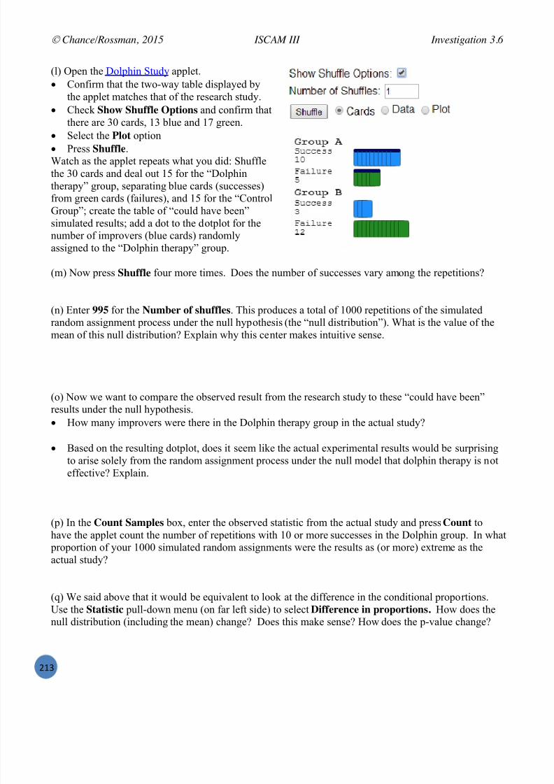
7/25/2019 Text: Investigating Statistical Concepts, Applications, and Methods
http://slidepdf.com/reader/full/text-investigating-statistical-concepts-applications-and-methods 214/428
Chance/Rossman, 2015 ISCAM III Investigation 3.6
!W#
(l) Open the Dolphin Study applet. Confirm that the two-way table displayed by
the applet matches that of the research study. Check Show Shuffle Options and confirm that
there are 30 cards, 13 blue and 17 green.
Select the Plot option Press Shuffle .
Watch as the applet repeats what you did: Shufflethe 30 cards and deal out 15 for the “Dolphin therapy” group, separating blue cards (successes)from green cards (failures), and 15 for the “Contro lGroup”; create the table of “could have been”simulated results; add a dot to the dotplot for thenumber of improvers (blue cards) randomlyassigned to the “Dolphin therapy” group.
(m) Now press Shuffle four more times. Does the number of successes vary among the repetitions?
(n) Enter 995 for the Number of shuffles . This produces a total of 1000 repetitions of the simulatedrandom assignment process under the null hypothesis (the “null distribution”) . What is the value of themean of this null distribution? Explain why this center makes intuitive sense.
(o) Now we want to compare the observed result from the research study to these “could have been”
results under the null hypothesis. How many improvers were there in the Dolphin therapy group in the actual study?
Based on the resulting dotplot, does it seem like the actual experimental results would be surprisingto arise solely from the random assignment process under the null model that dolphin therapy is noteffective? Explain.
(p) In the Count Samples box, enter the observed statistic from the actual study and press Count tohave the applet count the number of repetitions with 10 or more successes in the Dolphin group. In what
proportion of your 1000 simulated random assignments were the results as (or more) extreme as theactual study?
(q) We said above that it would be equivalent to look at the difference in the conditional proportions.Use the Statistic pull-down menu (on far left side) to select Difference in proportions. How does thenull distribution (including the mean) change? Does this make sense? How does the p-value change?
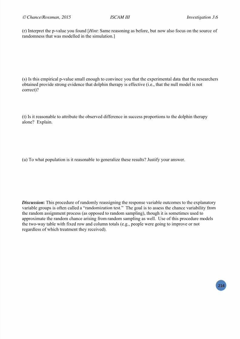
7/25/2019 Text: Investigating Statistical Concepts, Applications, and Methods
http://slidepdf.com/reader/full/text-investigating-statistical-concepts-applications-and-methods 215/428
Chance/Rossman, 2015 ISCAM III Investigation 3.6
!WP
(r) Interpret the p-value you found [ Hint : Same reasoning as before, but now also focus on the source ofrandomness that was modelled in the simulation.]
(s) Is this empirical p-value small enough to convince you that the experimental data that the researchersobtained provide strong evidence that dolphin therapy is effective (i.e., that the null model is notcorrect)?
(t) Is it reasonable to attribute the observed difference in success proportions to the dolphin therapyalone? Explain.
(u) To what population is it reasonable to generalize these results? Justify your answer.
Discussion : This procedure of randomly reassigning the response variable outcomes to the explanatoryvariable groups is often called a “randomization test.” The goal is to assess the chance variability fromthe random assignment process (as opposed to random sampling), though it is sometimes used toapproximate the random chance arising from random sampling as well. Use of this procedure modelsthe two-way table with fixed row and column totals (e.g., people were going to improve or notregardless of which treatment they received).

7/25/2019 Text: Investigating Statistical Concepts, Applications, and Methods
http://slidepdf.com/reader/full/text-investigating-statistical-concepts-applications-and-methods 216/428
Chance/Rossman, 2015 ISCAM III Investigation 3.6
!WR
0+456 )'*7$4,8'*,Due to the small p-value (0.01 < p-value < 0.05) from our “randomization test ,” we have moderatelystrong evidence that “luck of the draw” of the random assignment process alone is not a reasonableexplanation for the higher proportion of subjects who substantially improved in the dolphin therapygroup compared to the control group. Thus the researchers have moderate evidence that subjects aged
18 – 65 with a clinical diagnosis of mild to moderate depression (who would apply for such a study andfit the inclusion criteria) will have a higher probability of substantially reducing their depressionsymptoms if they are allowed to swim with dolphins rather than simply visiting and swimming inHonduras. Because this was a randomized comparative experiment, we can conclude that there ismoderately strong evidence that swimming with dolphins causes a higher probability of experiencingsubstantial improvement in depression symptoms. But with this volunteer sample, we should becautious about generalizing this conclusion beyond the population of people suffering from mild-to-moderate depression who could afford to take the time to travel to Honduras for two weeks.
9:"7+87% 9:'#$%; TDY< A recent study compared two groups: One group was reminded of the sacrifices that physicians have tomake as part of their training, and the other group was given no such reminder. All physicians in thestudy were then asked whether they consider it acceptable for physicians to receive free gifts fromindustry representatives. It turn ed out that 57/120 in the “sacrifice reminders” group answered that giftsare acceptable, compared to 13/60 in the “no reminder” group.(a) Identify the explanatory and response variables in this study.(b) Do you believe this study used random assignment? What would that involve?(c) Do you believe this study used random sampling? What would that involve?(d) Explain how you would carry out a simulation analysis to approximate a p-value for this study.[ Hint : How many cards? How many of each type? How many would you deal out? What would yourecord? How would you find the p-value?](e) A colleague points out that the sample sizes are not equal in this study, so we can’t dr aw meaningfulconclusions. How should you respond?
9:"7+87% 9:'#$%; TDYC How would you find a two-sided p-value for the dolphin study?

7/25/2019 Text: Investigating Statistical Concepts, Applications, and Methods
http://slidepdf.com/reader/full/text-investigating-statistical-concepts-applications-and-methods 217/428
Chance/Rossman, 2015 ISCAM III Investigation 3.7
!WS
Investigation 3.7: Is Yawning Contagious?
The folks at MythBusters , a popular television program on the Discovery Channel, investigated whetheryawning is contagious by recruiting fifty subjects at a local flea market and asking them to sit in one ofthree small rooms for a short period of time. For some of the subjects, the attendee yawned while
leading them to the room (planting a yawn “seed”), whereas for other subjects the attendee did notyawn. As time passed, the researchers watched (via a hidden camera) to see which subjects yawned.
(a) Identify the explanatory variable (EV) and the response variable (RV) in this study.
EV:
RV:
(b) Define the relevant parameter of interest, and state the null and alternative hypotheses for this study.Be sure to clearly define any symbols that you use.
Parameter:
H0:
Ha:
In the study they found that 10 of 34 subjects who had been given a yawn seed actually yawnedthemselves, compared with 4 of 16 subjects who had not been given a yawn seed.
(c) More people yawned in the “seed” group (10 vs. 4), but this comparison is not meaningful by itself.Why not, and what would be a better comparison to make?
(d) Create a two-table table summarizing the results, using the explanatory variable as the columnvariable .
Totals
Totals
(e) Explain what will change about the simulation used to find an empirical p-value in this study ascompared to the Dolphin Therapy study.

7/25/2019 Text: Investigating Statistical Concepts, Applications, and Methods
http://slidepdf.com/reader/full/text-investigating-statistical-concepts-applications-and-methods 218/428
Chance/Rossman, 2015 ISCAM III Investigation 3.7
!WT
(f) Open the Analyzing Two-way Tables applet. Paste in the raw data and press
Use Data or enter the titles andcounts of a two-way table and
press Use Table . (Or check the
2!
2 box and enter the cellvalues.) Check the Show Shuffle
Options box. Set Number of Shuffles to
1000 . Press Shuffle .
Briefly describe this randomization (null) distribution: What is its shape? What is the mean? What is thestandard deviation?
(g) Specify the observed value for the difference in the conditional proportions in the Count Samples box. Then indicate whether the research conjecture expected a larger or smaller proportion of successesin Group A by choosing Greater Than or Less Than from the pull-down menu. Then press the Count
button.
/A"7+ ?\F"$4% The simulations you have conducted in Investigations 3.6 (Dolphin Therapy) and above approximatedthe p-value for two-way tables arising from random assignment by assuming the row and column totalsare fixed. In this case, the probability of obtaining a specific number of successes in one group can becalculated exactly using the hypergeometric probability distribution. (We used the independent binomial distributions with the teen hearing loss study, where we wanted to sample separately from two
populations and the overall number of successes was not fixed in advance.)
Keep in mind, that under the null hypothesis, we are assuming the group assignments made nodifference and that there would be 14 successes (“yawners”) and 36 failures (“non -yawners”) betweenthe two groups regardless.
Because the random assignment makes every configuration of the subjects between the two groupsequally likely, we determine the probability of any particular outcome for the number of yawners andnon-yawners by first counting the total number of ways to assign 34 of the subjects to the yawn-seedgroup (and 16 to the no-yawn-seed group) in the denominator. The numerator is then the number ofways to get a particular set of configurations for that group, such as those consisting of 10 yawners and24 non-yawners.

7/25/2019 Text: Investigating Statistical Concepts, Applications, and Methods
http://slidepdf.com/reader/full/text-investigating-statistical-concepts-applications-and-methods 219/428
Chance/Rossman, 2015 ISCAM III Investigation 3.7
!WU
(h) How many ways altogether are there to randomly assign these 50 subjects into one group of 34(yawn-seed group) and the remaining group of 16 (no-yawn-seed group)? [ Hint : Recall what you sawearlier with the binomial distribution and counting the number of ways to obtain S successes and Ffailures in n trials. See the Technical Details in Investigation 1.1.]
(i) Now consider the 14 successes and the 36 failures. How many ways are there to randomly select 10of the successes? How many ways are there to randomly assign 24 of the failures to be in the yawn seedgroup? How should you combine these two numbers to calculate the total number of ways to obtain 10successes and 24 failures in the yawn-seed group, the configuration that we observed in the study?
Successes Failures
Total:
(j) To determine the exact probability that random assignment would produce exactly 10 successes and24 failures into the group of 34 subjects, divide your calculation in (i) by your calculation in (h).
(k) Explain why your answer to (j) is not yet the p-value for this study.
Result: The probability of obtaining k successes in Group A, with n observations, when sampled from atwo-way table with N observations, consisting of M successes and N M failures is:
P(X = k ) = C( M , k ) ! C( N M , n k ) / C( N , n)where C( N , n) = N !/[n!( N n!)] is the number of ways to choose n items from a group of N items.X represents the number of successes randomly selected for group A. X is a hypergeometric random
variable. Also note E(X) = n( M / N ) and SD(X) = )]1(/[))(( 2 N N n N M N nM .
In this study, we had N = 50 subjects and we defined yawning to be success so M = 14. We alsoarbitrarily chose to focus on the yawn-seed group, so n = 34. This calculation works out the same if youhad defined “not yawning” to be a success and/or if you had focused on the 16 people in the no -yawn-seed group. You just need to make sure you count consistently.
We will continue to define the p-value to be the probability of obtaining results at least as extreme asthose observed in the actual study. Because we expected more yawners in the yawn-seed group, the p-value is the probability of randomly assigning at least 10 of the yawners in the yawn-seed group.

7/25/2019 Text: Investigating Statistical Concepts, Applications, and Methods
http://slidepdf.com/reader/full/text-investigating-statistical-concepts-applications-and-methods 220/428
Chance/Rossman, 2015 ISCAM III Investigation 3.7
!WV
So far you have found P(X = 10) = C(14, 10) ! C(36, 24) / C(50, 34) = 0.2545.
(l) Calculate P(X = 11), P(X = 12), P(X = 13), and P(X = 14) using the hypergeometric probabilityformula.
P(X = 11) P(X = 12)
P(X = 13) P(X = 14)
Why do we stop at 14?
(m) Sum all five probabilities together (including P(X = 10)) to determine the exact p-value for theyawning study. How does this p-value compare to the empirical p-value from the applet simulation?Write a one or two sentence interpretation of this p-value.
Exact p-value: Comparison:
Interpretation:
Definition: Using the hypergeometric probabilities to determine a p-value in this fashion for a two-waytable is called Fisher’s Exact Test , named after R. A. Fisher.
(n) Calculate this hypergeometric probability using technology (see Technology Detour on next page).
(o) Set up and carry out the calculation to determine the exact p-value where you define the success to be “not yawning” and the group of interest to be the yawn seed group.
(p) Set up and carry out the calculation to determine the exact p-value, where you focus on the numberthat did not yawn in the no-yawn-seed group. Show that you obtain the same exact p-value as before.
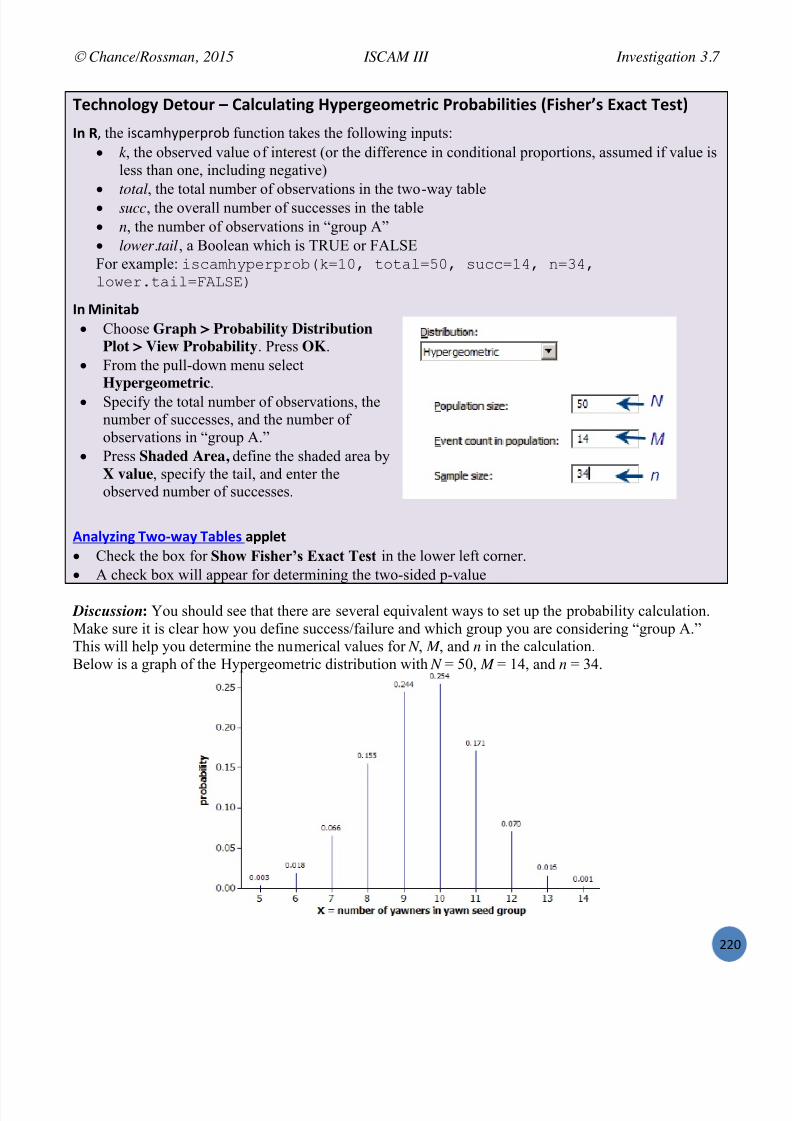
7/25/2019 Text: Investigating Statistical Concepts, Applications, and Methods
http://slidepdf.com/reader/full/text-investigating-statistical-concepts-applications-and-methods 221/428
Chance/Rossman, 2015 ISCAM III Investigation 3.7
!!X
!%7=*'$'>6 2%+'4: – Calculating Hypergeometric Probabilities (Fisher’s Exact Test)
M* @7the '()&*+68,5851= function takes the following inputs: k , the observed value of interest (or the difference in conditional proportions, assumed if value is
less than one, including negative)
total , the total number of observations in the two-way table succ , the overall number of successes in the table n, the number of observations in “group A” lower.tail , a Boolean which is TRUE or FALSE
For example: ?9IB0618;383CL&@!,-Q 7C7B4!_-Q 92II!,]Q <!(]Q4C>;3=7B?4!RSEK'*
M* B8*8+"# Choose Graph > Probability Distribution
Plot > View Probability . Press OK . From the pull-down menu select
Hypergeometric . Specify the total number of observations, the
number of successes, and the number ofobservations in “group A.”
Press Shaded Area, define the shaded area byX value , specify the tail, and enter theobserved number of successes.
<*"$6E8*> !G'\G"6 !"#$%, "??$%+ Check the box for Show Fisher’s Exact Test in the lower left corner. A check box will appear for determining the two-sided p-value
Discussion : You should see that there are several equivalent ways to set up the probability calculation.Make sure it is clear how you define success/failure and which group you are considering “group A.”This will help you determine the numerical values for N , M , and n in the calculation.Below is a graph of the Hypergeometric distribution with N = 50, M = 14, and n = 34.

7/25/2019 Text: Investigating Statistical Concepts, Applications, and Methods
http://slidepdf.com/reader/full/text-investigating-statistical-concepts-applications-and-methods 222/428
Chance/Rossman, 2015 ISCAM III Investigation 3.7
!!W
Using probability rules, you can show that the expected value of this distribution is n N M )/( =(14/50) ! 34 = 9.52 yawners in yawn seed group and the standard deviation of the probabilitydistribution is the square root of n ! ( M/N ) ! ( N – n)/ N ! ( N – M )/( N – 1) = 1.496 yawners.
(q) Compare this graph and the mean and standard deviation values to your simulation results.
(r) What conclusions will you draw from the p-value for this study?
(s) On the Mythbusters program, the hosts concluded that, based on the observed difference inconditional proportions and the large sample size, there is “ little doubt, yawning seems to becontagious.” Do you agree?
0+456 )'*7$4,8'*, With a large p-value of 0.513 (Fisher’s Exact Test), we do not have any evidence that the difference
between the two groups (with and without yawn seed) was not created by chance alone from the randomassignment process. If there was nothing to the theory that yawning is c ontagious, by “luck of the draw”alone, we would expect 10 or more of the yawners to end up in the yawn seed group in more than 50%of random assignments. Although the study results were in the conjectured direction, the difference
between the yawning proportions was not large enough to convince us that the probability of yawning istruly larger when a yawn seed is planted. The researchers could try the study again with a larger samplesize to increase the power of their test. The researchers also may want to be cautious in generalizing
these results beyond the population of volunteers at a local flea market. It’s also not clear hownaturalistic the setting of leading individuals to a small room to wait is.
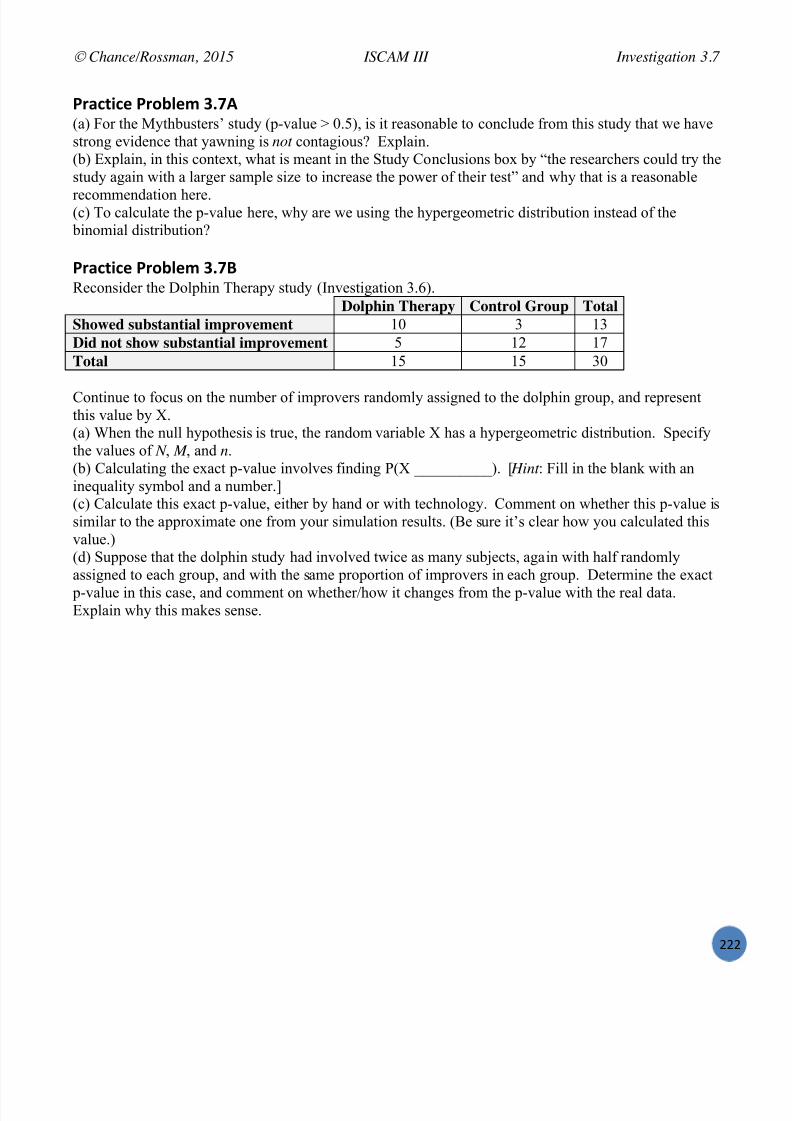
7/25/2019 Text: Investigating Statistical Concepts, Applications, and Methods
http://slidepdf.com/reader/full/text-investigating-statistical-concepts-applications-and-methods 223/428
Chance/Rossman, 2015 ISCAM III Investigation 3.7
!!!
9:"7+87% 9:'#$%; TDZ< (a) For the Mythbusters’ study (p -value > 0.5), is it reasonable to conclude from this study that we havestrong evidence that yawning is not contagious? Explain.(b) Explain, in this context, what is meant in the Study Co nclusions box by “the researchers could try thestudy again with a larger sample size to increase the power of their test” and why that is a reasonable
recommendation here.(c) To calculate the p-value here, why are we using the hypergeometric distribution instead of the
binomial distribution?
9:"7+87% 9:'#$%; TDZC Reconsider the Dolphin Therapy study (Investigation 3.6).
Dolphin Therapy Control Group TotalShowed substantial improvement 10 3 13Did not show substantial improvement 5 12 17Total 15 15 30
Continue to focus on the number of improvers randomly assigned to the dolphin group, and representthis value by X.(a) When the null hypothesis is true, the random variable X has a hypergeometric distribution. Specifythe values of N , M , and n.(b) Calculating the exact p-value involves finding P(X __________). [ Hint : Fill in the blank with aninequality symbol and a number.](c) Calculate this exact p-value, either by hand or with technology. Comment on whether this p-value issimilar to the a pproximate one from your simulation results. (Be sure it’s clear how you calculated thisvalue.)(d) Suppose that the dolphin study had involved twice as many subjects, again with half randomlyassigned to each group, and with the same proportion of improvers in each group. Determine the exact
p-value in this case, and comment on whether/how it changes from the p-value with the real data.Explain why this makes sense.

7/25/2019 Text: Investigating Statistical Concepts, Applications, and Methods
http://slidepdf.com/reader/full/text-investigating-statistical-concepts-applications-and-methods 224/428
Chance/Rossman, 2015 ISCAM III Investigation 3.8
!!#
Investigation 3.8: CPR vs. Chest Compressions
For many years, if a person experienced a heart attack and a bystander called 911, the dispatcherinstructed the bystander in how to administer chest compression plus mouth-to-mouth ventilation (acombination known as CPR) until the emergency team arrived. Some researchers believe that giving
instruction in chest compression alone (CC) would be a more effective approach. In the 1990s, arandomized study was conducted in Seattle involving 518 cases (Hallstrom, Cobb, Johnson, & Copass, New England Journal of Medicine , 2000). In 278 cases, the dispatcher gave instructions in standard CPRto the bystander, and in the remaining 240 cases the dispatcher gave instructions in CC alone. A total of64 patients survived to discharge from the hospital: 29 in the CPR group and 35 in the CC group.
(a) Identify the observational units, explanatory variable, and response variable. Is this an observationalstudy or an experiment?
Observational units:
Explanatory:Response:
Type of study: Observational Experimental
(b) Construct a two-way table to summarize the results of this study. Remember to put the explanatoryvariable in the columns.
(c) Calculate the difference in the conditional proportions who survived (CC – CPR). Does this seem to be a noteworthy difference to you?
(d) Use techn ology to carry out Fisher’s Exact Test (by calculating the corresponding hypergeometric probability) to assess the strength of evidence that the probability of survival is higher with CC alone ascompared to standard CPR. Write out how to calculate this probability, report the p-value, and interpret(on the next page) what it is the probability of.
p-value = P(X ) =where X follows a hypergeometric distribution with N = , M = , and n =

7/25/2019 Text: Investigating Statistical Concepts, Applications, and Methods
http://slidepdf.com/reader/full/text-investigating-statistical-concepts-applications-and-methods 225/428
Chance/Rossman, 2015 ISCAM III Investigation 3.8
!!P
Interpretation:
Because the sample sizes are large in this study, you should not be surprised that the distribution you
examined in (d) is approximately normal. The large sample sizes allow us to approximate thehypergeometric distribution with a normal distribution. Thus, with large samples sizes (e.g., at least 5successes and at least 5 failures in each group), an alternative to Fisher’s Exact Test is the two -sample z-test that you studied in Section 3.1.
(e) Use technology to obtain the two-sample z-test statistic and p-value for this study. Compare this p-value to the one from Fisher’s Exact Test; are they similar?
(f) Suggest a way of improving the approximation of the p-value.
(g) (Optional): Compare the normal approximation with a continuity correction to the hypergeometriccalculation. [ Hints: @. [7 use '()&*+68,5.15*F!V7 RWU7 SP7 !TU7 I[ZfG 15 2(, %+, 0.&-6K'.3 I<1:<&6I&=-,( &88-,% to compare the normal approximation to the hypergeometric calculation.]
(h) Do the data from this study provide convincing evidence that CC alone is better than standard CPRat the 10% significance level? Explain. How about the 5% level of significance?
(i) An advantage to using the z-procedures is being able to easily produce a confidence interval for the parameter. Use technology to determine a 90% confidence interval for the parameter of interest, andthen interpret this interval. [ Hint : Think carefully about what the relevant parameter is in this study.]

7/25/2019 Text: Investigating Statistical Concepts, Applications, and Methods
http://slidepdf.com/reader/full/text-investigating-statistical-concepts-applications-and-methods 226/428
Chance/Rossman, 2015 ISCAM III Investigation 3.8
!!R
(j) Suppose you had defined the parameter by subtracting in the other direction (e.g., CPR – CC insteadof CC – CPR). How would that change:
(i) the observed statistic?
(ii) the test statistic?
(iii) the p-value?
(iv) confidence interval?
9:"7+87% 9:'#$%; TD[(a) Researchers in the CPR study also examined other response variables. For example, the 911dispatcher’s instructions were completely delivered in 62% of episodes assigned to chest compression
plus mouth-to-mouth compared to 81% of the episodes assigned to chest compression alone.
(i) Calculate the difference in conditional proportions and compare it to the original study.(ii) Without calculating, do you suspect the p-value for comparing this new response variable between the two groups will be larger or smaller or about the same as the p-value youdetermined above? Explain your reasoning.
(b) The above study was operationally identical to that of another study and the results of the two studieswere combined. Of the 399 combined patients randomly assigned to standard CPR, 44 survived todischarge from the hospital. Of the 351 combined patients randomly assigned to chest compressionalone, 47 survived to discharge.
(i) Calculate the difference in conditional proportions and compare it to the original study.(ii) Without calculating, do you suspect the p-value for this comparison will be larger, smaller, or
the same as the p-value you determined? Explain your reasoning.
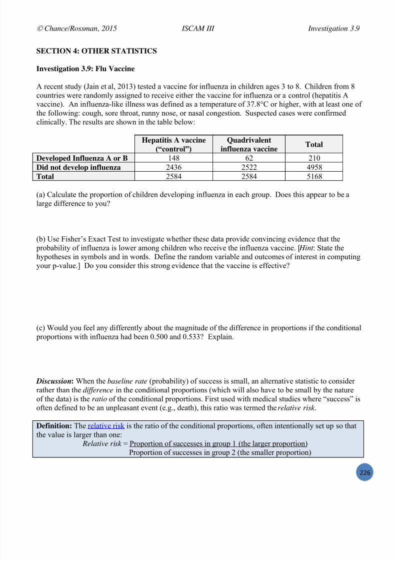
7/25/2019 Text: Investigating Statistical Concepts, Applications, and Methods
http://slidepdf.com/reader/full/text-investigating-statistical-concepts-applications-and-methods 227/428
Chance/Rossman, 2015 ISCAM III Investigation 3.9
!!S
SECTION 4: OTHER STATISTICS
Investigation 3.9: Flu Vaccine
A recent study (Jain et al, 2013) tested a vaccine for influenza in children ages 3 to 8. Children from 8
countries were randomly assigned to receive either the vaccine for influenza or a control (hepatitis Avaccine). An influenza-like illness was defined as a temperature of 37.8°C or higher, with at least one ofthe following: cough, sore throat, runny nose, or nasal congestion. Suspected cases were confirmedclinically. The results are shown in the table below:
Hepatitis A vaccine(“control”)
Quadrivalentinfluenza vaccine Total
Developed Influenza A or B 148 62 210Did not develop influenza 2436 2522 4958Total 2584 2584 5168
(a) Calculate the proportion of children developing influenza in each group. Does this appear to be alarge difference to you?
(b) Use Fisher’s Exact Test to investigate whether these data provide convincing evidence that the probability of influenza is lower among children who receive the influenza vaccine. [ Hint : State thehypotheses in symbols and in words. Define the random variable and outcomes of interest in computingyour p-value.] Do you consider this strong evidence that the vaccine is effective?
(c) Would you feel any differently about the magnitude of the difference in proportions if the conditional proportions with influenza had been 0.500 and 0.533? Explain.
Discussion : When the baseline rate (probability) of success is small, an alternative statistic to consider
rather than the difference in the conditional proportions (which will also have to be small by the natureof the data) is the ratio of the conditional proportions. First used with medical studies where “success” isoften defined to be an unpleasant event (e.g., death), this ratio was termed the relative risk .
Definition: The relative risk is the ratio of the conditional proportions, often intentionally set up so thatthe value is larger than one:
Relative risk = Proportion of successes in group 1 (the larger proportion)Proportion of successes in group 2 (the smaller proportion)

7/25/2019 Text: Investigating Statistical Concepts, Applications, and Methods
http://slidepdf.com/reader/full/text-investigating-statistical-concepts-applications-and-methods 228/428
Chance/Rossman, 2015 ISCAM III Investigation 3.9
!!T
The relative risk tells us how many times higher the “risk” or “likelihood” of “success” is in group 1compared to group 2.
(d) Determine and interpret the ratio of the conditional proportions who developed influenza betweenthe control and vaccinated groups in this study.
(e) Because we are now working with a ratio, we can also interpret this in terms of percentage change .Subtract one from the relative risk value and multiply by 100% to determine what percentage higher the
proportion who developed influenza is in the control group compared to the vaccine group.
Note: The efficacy of a vaccine is defined as (1 vaccinated risk /unvaccinated risk ) ! 100%.
Of course, now we would also like a confidence interval for the corresponding parameter, the ratio ofthe underlying probabilities of survival between these two treatments. When we produced confidenceintervals for other parameters, we examined the sampling distribution of the corresponding statistic tosee how values of that statistic varied under repeated random sampling. So now let’s examine the
behavior of the relative risk of conditional proportions using the Analyzing Two-Way Tables applet tosimulate the random assignment process (as opposed to simulating the random sampling from a
binomial process) under t he (null) assumption that there’ s no difference between the two treatments.[See the Technology Detour below for equivalent R/Minitab instructions.]
(f) Generate a null distribution for Relative Risks: Check the 2! 2 box Enter the two-way table into the applet and press Use Table . Generate 1000 random shuffles. This will take some time! Use the Statistic pull-down menu to select Relative Risk.
Describe the behavior of the null distribution of relative risk values.
(g) Where does the observed value of the relative risk from the actual study fall in the null distribution
of the relative risks? What proportion of the simulated relative risks are at least this extreme?
(h) What percentage of the simulated relative risks are larger than 1.28 (just so you have a non-zerovalue to compare to later)?

7/25/2019 Text: Investigating Statistical Concepts, Applications, and Methods
http://slidepdf.com/reader/full/text-investigating-statistical-concepts-applications-and-methods 229/428
Chance/Rossman, 2015 ISCAM III Investigation 3.9
!!U
But can we apply a mathematical model to this distribution?
(i) Why does it make sense that the mean of the simulated relative risks is close to the value 1? [ Hint :Remember the assumption behind your simulation analysis.]
(j) You should notice some slight skewness in the distribution of relative risk values. Explain why youwouldn’t be surprised for the distribution of this statistic to be skewed to the right (especially withsmaller sample sizes).
(k) In fact, this distribution is usually well modeled by a log normal distribution. To verify this, check
the ln relative risk box (in the lower left corner) to take the natural log of each relative risk value anddisplay a new histogram of these transformed values. Describe the shape of this distribution. Is thedistribution of the lnrelrisk well modeled by a normal distribution?
(l) What is the mean of the simulated lnrelrisk values? Why does this value make sense?
(m) What is the standard deviation of the lnrelrisk values?
(n) Calculate the observed value of ln( pˆ
1/ pˆ
2) for this study. Where does this value fall (near in themiddle or in the tail) of this simulated distribution of lnrelrisk values? Has the empirical p-valuechanged?
(o) If you found the empirical p-value using ln( pˆ
1/ pˆ
2), it would be identical to the empirical p-value
found in (i). Why? What did change about the distribution? [ Hint : What percentage of the simulated lnrel risk values are more extreme than ln(1.28), how does this compare to (h)?]

7/25/2019 Text: Investigating Statistical Concepts, Applications, and Methods
http://slidepdf.com/reader/full/text-investigating-statistical-concepts-applications-and-methods 230/428

7/25/2019 Text: Investigating Statistical Concepts, Applications, and Methods
http://slidepdf.com/reader/full/text-investigating-statistical-concepts-applications-and-methods 231/428
Chance/Rossman, 2015 ISCAM III Investigation 3.9
!#X
(w) Is the midpoint of this confidence interval for the population relative risk equal to the observedvalue of the sample relative risk? Explain why this makes sense.
(x) Suppose you used this method to construct a confidence interval for each of the 1,000 simulatedrandom samples that you generated in (f). Do you expect the value 1 to be in these intervals? All ofthem? Most of them? What percentage of them? Explain.
(y) Compare the confidence interval you just calculated to the one given by the applet if you now checkthe 95% CI for relative risk box.
0+456 )'*7$4,8'*, This study provided very strong evidence that children who receive the QIV vaccine are less likely to
develop influenza than those who receive a control vaccine (exact one-sided p-value < 0.001, z-score =6.08). An approximate 95% confidence interval for the difference in the probabilities indicates that the
probability of influenza (of any severity) is 0.023 to 0.044 (2.3 to 4.4 percentage points) lower whenreceiving the QIV vaccine.
However, focusing on the difference in “success” probabilities has some limitations. In particular, ifthe probabilities are small it may be difficult for us to interpret the magnitude of the difference betweenthe values. Also, we have to be very careful with our language, focusing on the difference in the
influenza probabilities and not the percentage change. An alternative to examining a confidence intervalfor the difference in the conditional probabilities is to construct a confidence interval for the relative risk(ratio of conditional probabilities). A large sample approximation exists for a z-interval for theln(relative risk) which can then be back-transformed to an interval for long-run relative risk. Many
practitioners prefer focusing on this ratio parameter rather than the difference. From this study, we are95% confident that ratio of the influenza probabilities is between 1.78 and 3.19. This means thatreceiving the placebo rather than the real vaccine raises the probability of developing influenza by
between 78% and 219%.An alternative would be to calculate the ratio in the other direction, using the relative risk of
developing influenza between the vaccinated group compared to the unvaccinated group ( 2ˆ
p 2/ 1ˆ
p =0.4189). This approach is called examining the “efficacy” of the vaccination. Using the same standard
error, a 95% confidence interval for the long-run relative risk is (0.313, 0.561). This means we are 95%confident that the use of the QIV vaccine reduces the probability of developing influenza by between(100 56.1) = 44% and (100 31.3) = 69%. In other words, we are 95% confident that the efficacy ofthe QIV vaccine in the larger population of children aged 3-8 years is between 44% and 69%.
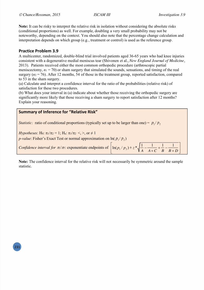
7/25/2019 Text: Investigating Statistical Concepts, Applications, and Methods
http://slidepdf.com/reader/full/text-investigating-statistical-concepts-applications-and-methods 232/428
Chance/Rossman, 2015 ISCAM III Investigation 3.9
!#W
Note: It can be risky to interpret the relative risk in isolation without considering the absolute risks(conditional proportions) as well. For example, doubling a very small probability may not benoteworthy, depending on the context. You should also note that the percentage change calculation andinterpretation depends on which group (e.g., treatment or control) is used as the reference group.
9:"7+87% 9:'#$%; TD]A multicenter, randomized, double-blind trial involved patients aged 36-65 years who had knee injuriesconsistent with a degenerative medial meniscus tear (Shivonen et al., New England Journal of Medicine , 2013). Patients received either the most common orthopedic procedure (arthroscopic partialmeniscectomy, n1 = 70) or sham surgery that simulated the sounds, sensations, and timing of the realsurgery ( n2 = 76). After 12 months, 54 of those in the treatment group, reported satisfaction, comparedto 53 in the sham surgery.(a) Calculate and interpret a confidence interval for the ratio of the probabilities (relative risk) ofsatisfaction for these two procedures.(b) What does your interval in (a) indicate about whether those receiving the orthopedic surgery aresignificantly more likely that those receiving a sham surgery to report satisfaction after 12 months?Explain your reasoning.
Summary of Inference for “Relative Risk”
Statistic: ratio of conditional proportions (typically set up to be larger than one) = 1
ˆ
p / 2
ˆ
p
Hypotheses : H0: 1/ 2 = 1; H a: 1/ 2 <, >, or ≠ 1 p-value : Fisher’s Exact Test or normal approximation on ln( 1
ˆ
p / 2
ˆ
p )
Confidence interval for 1/ 2: exponentiate endpoints of
D B BC A A
z p p 1111
*)ˆ
/ˆ
ln( 21
Note: The confidence interval for the relative risk will not necessarily be symmetric around the samplestatistic.

7/25/2019 Text: Investigating Statistical Concepts, Applications, and Methods
http://slidepdf.com/reader/full/text-investigating-statistical-concepts-applications-and-methods 233/428
Chance/Rossman, 2015 ISCAM III Investigation 3.9
!#!
!%7=*'$'>6 2%+'4: – 08;4$"+8*> @"*5'; <,,8>*;%*+
We can select observations from a hypergeometric distribution for the cell 1 counts and then computethe cell 2 counts and the number of failures based on the fixed row and column totals. With thisinformation you can compute the difference in conditional proportions, relative risk, etc. We should howto calculate p
ˆ
unvac below, the rest is up to you. Also keep in mind you can use “log” to calculate thenatural logs of values. Also recall how you created a Boolean expression in Investigation 3.1 to find the
p-value from the simulated results.
M* @ > VBIY<G"C2<7!3618;3&,----Q #,-Q ]ba_Q #_a]*
210 is the number of successes ( M ) 4985 is the number of failures ( N M) 2584 is the sample size ( n)
> J<HBIY<G"C2<7 ! #,-)VBIY<G"C2<7> J<HBI86B7 ! J<HBIY<G"C2<7$#_a]
M* B8*8+"# Choose Calc > Random Data > Hypergeometric
Number of rows: 10000Store samples in column: VBIY<G"C2<7 Enter the name you want for the column and specify N , M , and n
Choose Calc > Calculator , store in nJ<HBIY<G"C2<7n , expression: ,a()nJ<HBII"C2<7n Choose Calc > Calculator , store in nJ<HBI86B7n , expression: nJ<HBII"C2<7n$#_a]

7/25/2019 Text: Investigating Statistical Concepts, Applications, and Methods
http://slidepdf.com/reader/full/text-investigating-statistical-concepts-applications-and-methods 234/428
Chance/Rossman, 2015 ISCAM III Investigation 3.10
!##
Investigation 3.10: Smoking and Lung Cancer
After World War II, evidence began mounting that there was a link between cigarette smoking and pulmonary carcinoma (lung cancer). In the 1950s, three now classic articles were published on the topic.One of these studies was conduct ed in the United States by Wynder and Graham (“Tobacco Smoking as
a Possible Etiologic Factor in Bronchiogenic Cancer,” 1950, Journal of the American Medical Association ). They found records from a large number of patients with a specific type of lung cancer inhospitals in California, Colorado, Missouri, New Jersey, New York, Ohio, Pennsylvania, and Utah. Ofthose in the study, the researchers focused on 605 male patients with this form of lung cancer. Another780 male hospital patients with similar age and economic distributions without this type of lung cancerwere interviewed in St. Louis, Boston, Cleveland, and Hines, IL. Subjects (or family members) wereinterviewed to assess their smoking habits, occupation, education, etc. The table below classifies them asnon-smoker or light smoker, or at least a moderate smoker.
`6*5%: "*5 N:"=";None or Light smoker
(0-9 per day)
Moderate to Heavy smoker
(10-35+ per day)Total
Lung cancer patients 22 583 605Controls 204 576 780Total 226 1159 1385
(a) Calculate and interpret the relative risk of being a lung cancer patient for the moderate to heavy(“regular”) smokers compared to the None or Light “non -smokers.”
(b) Does this feel like an impressive statistic to you? Do you think it will be statistically significant?
(c) What is the estimate of the baseline rate of lung cancer from this table? Does that seem to be areasonable estimate to you? How is this related to the design of the study?
(d) Calculate and interpret the relative risk of being a control patient for the non-smokers compared tothe regular smokers. How does this compare to (a) and (b)?

7/25/2019 Text: Investigating Statistical Concepts, Applications, and Methods
http://slidepdf.com/reader/full/text-investigating-statistical-concepts-applications-and-methods 235/428
Chance/Rossman, 2015 ISCAM III Investigation 3.10
!#P
Definition: There are three main types of observational studies. Cross-classification study . The researchers categorize subjects according to both the explanatory
and the response variable simultaneously. For example, they could take a sample of adult malesand simultaneously record both their smoking status and whether they have lung cancer. Acommon design is cross-sectional , where all observations are taken at a fixed point in time.
Cohort study. The researchers identify individuals according to the explanatory variable and thenobserve the outcomes of the response variable. These are usually prospective designs and mayeven follow the subjects (the cohort ) for several years.
Case-control study . The researchers identify observational units in each response variable category(the “cases” and the “controls”) and then determine the explanatory variable outcome for eachobservational unit. How the controls are selected is very important in determining thecomparability of the groups. These are often retrospective designs in that the researchers may needto “look back” at historical data on the observational units.
(e) Would you classify the Wynder & Graham study as cross-classified, cohort, or case-control?Explain.
(f) Explain why using the relative risk (or even the difference in proportions) as the statistic can be problematic with case-control studies.
An advantage of case- control studies is when you are studying a “rare event,” you can ensure a largeenough numbe r of “successes” and fairly balanced group sizes. However, a disadvantage is that it does
not make sense to calculate “risk” or likelihood of success from a case -control study, because thedistribution of the response variable has been manipulated/determined by the researcher. Switching theroles of the explanatory and response often gives very different results for relative risk (changing ourmeasure of the strength of the relationship) and often really isn’t the comparison of interest stated by theresearch question. Consequently , conditional proportions of success and relative risk are notappropriate statistics to use with case-control studies . Instead, we will consider another way tocompare the uncertainty of an outcome between two groups.
Definition: The odds of success are defined as the ratio of the proportion of “successes” to the proportion of “failures ,” which simplifies to the ratio of the number of success es to failures.
groupthein failuresof number
grouptheinsuccessesof number
groupthein failuresof proportion
grouptheinsuccessesof proportionodds
For example, if the odds are 2-to-1 in favor of an outcome, we expect a success twice as often as afailure in the long run, so this corresponds to a probability of 2/3 of the outcome occurring. Similarly, ifthe probability of success is 1/10, then the odds equals (1/10)/(9/10) = 1/9, and failures is 9 times morelikely than success. It’s important to note how the “outcome” is defined. For example, in horse racing,odds are typically presented in terms of “losing the race,” so if a horse is given 2 -to-1 odds againstwinning a race, we expect the horse to lose two-thirds of the races in the long run.

7/25/2019 Text: Investigating Statistical Concepts, Applications, and Methods
http://slidepdf.com/reader/full/text-investigating-statistical-concepts-applications-and-methods 236/428
Chance/Rossman, 2015 ISCAM III Investigation 3.10
!#R
Definition: The odds ratio is another way to compare conditional proportions in a 2 ! 2 table.Odds ratio = (number of successes in group 1/number of failures in group 1)
(number of successes in group 2/number of failures in group 2)Like relative risk, if the odds ratio is 3, this is interpreted as “the odds of success in the ‘top’ group are 3times (or 200%) higher than the odds of success in the ‘bottom’ group.” However, the relative risk and
the odds ratio are not always similar in value.
(g) Calculate and interpret the odds ratio comparing the odds of lung cancer for the smokers to the oddsof lung cancer for the control group. Does this match (a)?
(h) Calculate and interpret the odds ratio for being in the control group for the non-smokers compared tothe smokers? Does this match (d) or (g)?
Key Results: A major disadvantage to relative risk is that your (descriptive) measure of the strength ofevidence that one group is “better” depends on which outcome you define a success as well as whichvariable you treat as the explanatory and which as the response. But a big advantage to odds ratio is thatit is invariant to these definitions (If your odds are 10 times higher to die from lung cancer if you are asmoker, then your odds of being a smoker are 10 times higher if you died from lung cancer). The onlyreal disadvantage is that the odds ratio is trickier to interpret (“higher odds” vs. the more natural “morelikely”). Thus, for case -control studies in particular, the odds ratio is the preferred statistic. However,when the success proportions are both small, the odds ratio can be used to approximate the relative risk.
(i) Let (“tau”) represent the population odds ratio of having lung cancer for those who are regularsmokers compared to those who are not regular smokers, so = 1/(1 1)/( 2/(1 2)). State the nulland alternative hypotheses in terms of this parameter.
(j) Use Fisher’s Exact Test to calculate the p -value. (Note: We get the same p-value no matter whichstatistic we use, why is that?)
But we still need a confidence interval for this new parameter as well.

7/25/2019 Text: Investigating Statistical Concepts, Applications, and Methods
http://slidepdf.com/reader/full/text-investigating-statistical-concepts-applications-and-methods 237/428
Chance/Rossman, 2015 ISCAM III Investigation 3.10
!#S
Theoretical Result: The sampling distribution of the sample odds ratio also follow a log-normaldistribution like the relative risk (for any study design). Thus, we can construct a confidence interval forthe population/treatment log-odds ratio using the normal distribution. The standard error of the samplelog-odds ratio (using the natural log) is given by the expression:
SE (ln odds ratio ) = DC B A
1111
where A, B, C , and D are the four table counts.
(k) Calculate this standard error and then use it to find an approximate 95% confidence interval for thelog odds ratio.
(l) Back-transform the end-points of the interval and (k) and interpret your results.
(m) Does your interval contain the value one? Discuss the implications of whether or not the intervalcontains the value one.
(n) Compare your results to the following R output:
(o) Summarize (with justification) the conclusions you would draw from this study (using both the p-value and the confidence interval, and addressing both the population you are willing to generalize toand whether or not you are drawing a cause-and-effect conclusion).
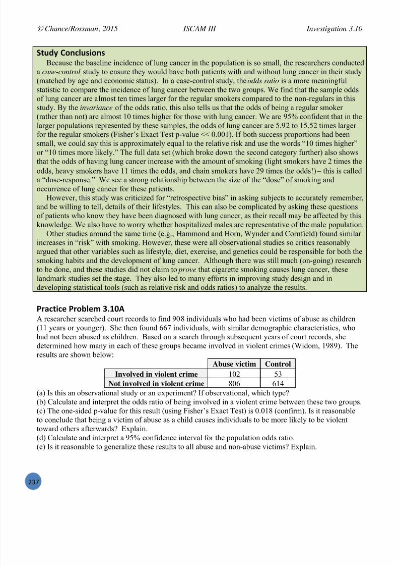
7/25/2019 Text: Investigating Statistical Concepts, Applications, and Methods
http://slidepdf.com/reader/full/text-investigating-statistical-concepts-applications-and-methods 238/428
Chance/Rossman, 2015 ISCAM III Investigation 3.10
!#T
0+456 )'*7$4,8'*,Because the baseline incidence of lung cancer in the population is so small, the researchers conducted
a case-control study to ensure they would have both patients with and without lung cancer in their study(matched by age and economic status). In a case-control study, the odds ratio is a more meaningfulstatistic to compare the incidence of lung cancer between the two groups. We find that the sample odds
of lung cancer are almost ten times larger for the regular smokers compared to the non-regulars in thisstudy. By the invariance of the odds ratio, this also tells us that the odds of being a regular smoker(rather than not) are almost 10 times higher for those with lung cancer. We are 95% confident that in thelarger populations represented by these samples, the odds of lung cancer are 5.92 to 15.52 times largerfor the regular smokers (F isher’s Exact Test p-value << 0.001). If both success proportions had beensmall, we could say this is approximately equal to the relative risk an d use the words “10 times higher”or “10 times more likely.” The full data set (which broke down the second category further) also showsthat the odds of having lung cancer increase with the amount of smoking (light smokers have 2 times theodds, heavy smokers have 11 times the odds, and chain smokers have 29 times the odds!) this is calleda “dose -response.” We see a strong relationship between the size of the “dose” of smoking andoccurrence of lung cancer for these patients.
However, this study was criticized for “retrospective bias” in asking subjects to accurately remember,and be willing to tell, details of their lifestyles. This can also be complicated by asking these questionsof patients who know they have been diagnosed with lung cancer, as their recall may be affected by thisknowledge. We also have to worry whether hospitalized males are representative of the male population.
Other studies around the same time (e.g., Hammond and Horn, Wynder and Cornfield) found similarincreases in “risk” with smoking. However, these were all observational studies so critics reasonablyargued that other variables such as lifestyle, diet, exercise, and genetics could be responsible for both thesmoking habits and the development of lung cancer. Although there was still much (on-going) researchto be done, and these studies did not claim to prove that cigarette smoking causes lung cancer, theselandmark studies set the stage. They also led to many efforts in improving study design and indeveloping statistical tools (such as relative risk and odds ratios) to analyze the results.
9:"7+87% 9:'#$%; TDHW<A researcher searched court records to find 908 individuals who had been victims of abuse as children(11 years or younger). She then found 667 individuals, with similar demographic characteristics, whohad not been abused as children. Based on a search through subsequent years of court records, shedetermined how many in each of these groups became involved in violent crimes (Widom, 1989). Theresults are shown below:
Abuse victim ControlInvolved in violent crime 102 53
Not involved in violent crime 806 614
(a) Is this an observational study or an experiment? If observational, which type?(b) Calculate and interpret the odds ratio of being involved in a violent crime between these two groups.(c) The one-sided p- value for this result (using Fisher’s Exact Test) is 0.018 (confirm). Is it reasonableto conclude that being a victim of abuse as a child causes individuals to be more likely to be violenttoward others afterwards? Explain.(d) Calculate and interpret a 95% confidence interval for the population odds ratio.(e) Is it reasonable to generalize these results to all abuse and non-abuse victims? Explain.

7/25/2019 Text: Investigating Statistical Concepts, Applications, and Methods
http://slidepdf.com/reader/full/text-investigating-statistical-concepts-applications-and-methods 239/428
Chance/Rossman, 2015 ISCAM III Investigation 3.10
!#U
9:"7+87% 9:'#$%; TDHWC(a) Suppose that individuals in Group 1 have a 2/3 probability of success, and those in Group 2 have a1/2 probability of success. Calculate and interpret the relative risk of success, comparing Group 1 toGroup 2.(b) Calculate and interpret the odds of success for Group 1.
(c) Calculate and interpret the odds ratio of success, comparing Group 1 to Group 2.(d) Suppose Group 3 has a 0.1 probability of success, and Group 4 has a 0.05 probability of success.Repeat questions (a) and (c).(e) In which case (Groups 1 and 2, or Groups 3 and 4) are the relative risk and odds ratio more similar?Why?
04;;":6 '( M*(%:%*7% (': -55, @"+8'
Statistic: ˆ = [ 1
ˆ
p /(1 1
ˆ
p )]/[ 2
ˆ
p /(1 2
ˆ
p )] = ( A ! D) / ( B ! C )(typically set up to be larger than one)
Hypotheses : H0: = 1; H a: <, >, or ≠ 1
p-value : Fisher’s Exact Test or normal approximation on ln( ˆ )
confidence interval for : exponential of DC B A
z 1111
*)ˆ
ln(
M* @I. G?96;3=7;97&0B73?[&I&BQ IQ LQ A*Q <3C>!#*Q B47 ! *
A BC D

7/25/2019 Text: Investigating Statistical Concepts, Applications, and Methods
http://slidepdf.com/reader/full/text-investigating-statistical-concepts-applications-and-methods 240/428
7/25/2019 Text: Investigating Statistical Concepts, Applications, and Methods
http://slidepdf.com/reader/full/text-investigating-statistical-concepts-applications-and-methods 241/428
Chance/Rossman, 2015 ISCAM III Investigation 3.11
!PX
0+"+8,+87"$ M*(%:%*7%(d) Outline the steps of a simulation that models the randomness in this study and helps you assess howunusual the statistic is that you calculated in (c) when the null hypothesis is true. Include a statement ofthe null and alternative hypotheses for your choice of parameter.
(e) Use technology to carry out your simulation and draw your conclusions. [ Hint : Be careful ofrounding issues in finding your p-value, make sure you are including observations as extreme as theobserved in your count.]
(f) Calculate and interpret a 95% confidence interval for your choice of parameter.
(g) Summarize (with justification) the conclusions you would draw from this study (using both the p-value and the confidence interval, and addressing both the population you are willing to generalize toand whether or not you are drawing a cause-and-effect conclusion).

7/25/2019 Text: Investigating Statistical Concepts, Applications, and Methods
http://slidepdf.com/reader/full/text-investigating-statistical-concepts-applications-and-methods 242/428
Chance/Rossman, 2015 ISCAM III Investigation 3.11
!PW
0+456 )'*7$4,8'*,The proportions of drivers who had not gotten a full night’s sleep in the previous week were 0.107 forthe case group of drivers who had been involved in a crash, compared to 0.075 for the control groupwho had not. Because these proportions are small, and because of the awkward roles of the explanatoryand response variables in this study (we would much rather make a statement about the proportion of
sleepless drivers who are involved in crashes), the odds ratio is a more meaningful statistic to calculate.The sample odds of having missed out o n a full night’s sleep were 1.59 times higher for the case groupthan for the control group. By the invariance of the odds ratio, we can also state that the sample odds ofhaving an accident are 1.59 times (almost 60%) higher for those who do not get a full night sleep thanthose who do. The empirical p-value (less than 5%) provides moderately strong evidence that such anextreme value for the sample odds ratio is unlikely to have arisen by chance alone if the proportion ofdrivers with sleepless nights was 0. 09 for both the population of “cases” and t he population of“controls.” (Using a one- sided Fisher’s Exact Test, we get p -value = 0.016.) A 95% confidence intervalfor the population odds ratio extends from 1.06 to 2.39 (1.04 to 2.45 with R). This interval providesstatistically significant evidence that the population odds ratio exceeds one and that, with 95%confidence, the odds of having an accident are about 1 to 2.5 times higher for the sleepy drivers than for
well rested drivers. We cannot attribute this association to a cause-and-effect relationship because thiswas an observational (case-control) study. We might also want to restrict our conclusions to NewZealand drivers.
9:"7+87% 9:'#$%; TDHHAnother landmark study on smoking began in 1952 (Hammond and Horn, 1958, “ Smoking and deathrates — Report on forty-four months of follow-up of 187, 783 men: II. Death rates by cause,” JAMA).They used 22,000 American Cancer Society volunteers as interviewers. Each interviewer was to ask 10healthy white men between the ages of 50 and 69 to complete a questionnaire on smoking habits. Eachyear during the 44-month follow-up, the interviewer reported whether or not the man had died, and if so,how. They ended up tracking 187,783 men in nine states (CA, IL, IA, MI, MN, NJ, NY, PA, WI).Almost 188,000 were followed up by the volunteers through October 1955, during which time about11,870 of the men had died, 488 from lung cancer. The following table classifies the men as having ahistory of regular cigarette smoking or not and whether or not they died from lung cancer . In this study,nonsmokers are grouped with occasional smokers, including pipe- and cigar-only smokers..";;'*5 "*5 .':*
Not regular smoker Regular smoker TotalLung cancer death 51 397 448
Alive or other cause of death 108,778 78,557 187,335Total 108,829 78,954 187,783
(a) Is this a case-control, cohort, or cross-classified study?(b) Calculate and interpret an odds ratio from the two-way table.(c) Produce and interpret a 95% confidence interval for the population odds ratio.(d) Are these results consistent with the Wynder and Graham study? Explain.

7/25/2019 Text: Investigating Statistical Concepts, Applications, and Methods
http://slidepdf.com/reader/full/text-investigating-statistical-concepts-applications-and-methods 243/428
Chance/Rossman, 2015 ISCAM III Example 3.1
!P!
Example 3.1: Wording of QuestionsTry these questions yourself before you use the solutions following to check your answers.
Researchers have conjectured that the use of the words “forbid” and “allow” can affect people’s!"#$%&#"# (% #)!*"+ ,)"#(-%&#. /()0"&(# -& 1& -&(!%0)2(%!+ #(1(-#(-2# 231## 4"!" !1&0%53+ 1##-6&"0 (%
1"! %&" %7 (8" 7%33%4-&6 ,)"#(-%	 /8%)30 +%)! 2%33"6" 133%4 #$""28"# %& 215$)# (81( 5-68( -&2-(" *-%3"&2": /8%)30 +%)! 2%33"6" 7%!;-0 #$""28"# %& 215$)# (81( 5-68( -&2-(" *-%3"&2":
<7 (8" == #()0"&(# 48% !"2"-*"0 (8" 7-!#( ,)"#(-%&> ? !"#$%&0"0 +"#. <7 (8" =@ #()0"&(# 48% !"2"-*"0 (8"#"2%&0 ,)"#(-%&> =A #1-0 &%.
B1C D0"&(-7+ (8" %;#"!*1(-%&13 )&-(# 1&0 (8" "E$31&1(%!+ 1&0 !"#$%&#" *1!-1;3"#.
B;C D# (8-# 1& %;#"!*1(-%&13 #()0+ %! 1& "E$"!-5"&(: D7 1& %;#"!*1(-%&13 #()0+> #)66"#( 1 $%("&(-132%&7%)&0-&6 *1!-1;3". D7 1& "E$"!-5"&(> "E$31-& (8" !%3"# %7 !1&0%5-F1(-%& 1&0 ;3-&0-&6 -& (8-# #()
B2C G%&#(!)2( 1 (4%H41+ (1;3" (% #)551!-F" (8"#" !"#)3(#.
B0C G%&#(!)2( 1 #"65"&("0 ;1! 6!1$8 (% 0-#$31+ (8"#" !"#)3(# 1&0 2%55"&( %& (8" !"31(-%-$ !"*"13"0 ;+ (8-# 6!1$8.
B"C I1#"0 %& "1!3-"! #()0-"#> !"#"1!28"!# "E$"2("0 $eople to be less likely to agree to “forbid” the#$""28"#> 3"10-&6 (% 5%!" &% !"#$%&#"# B1&0 (8)# 1$$"1!-&6 (% ;" -& 71*%! %7 81*-&6 (8" #$""28"#C>whereas they expected people to be comparatively less likely to agree to “allow” the speeches. J% (8"#"01(1 $!%*-0" #(!%&6 "*-0"&2" (81( (8"#" #()0"&(# !"#$%&0"0 5%!" $%#-(-*"3+ (%41!0 81*-&6 #)28 #$""28"#

7/25/2019 Text: Investigating Statistical Concepts, Applications, and Methods
http://slidepdf.com/reader/full/text-investigating-statistical-concepts-applications-and-methods 244/428
Chance/Rossman, 2015 ISCAM III Example 3.1
!P#
if their question was phrased in terms of “forbid” rather than “allow”? G1!!+ %)( 1 ("#( %7 #-6&-7-21&2"1&0 "E$31-& (8" 0"2-#-%& +%) 4%)30 51K" ;1#"0 %& (8" $H*13)". L!-(" 1 $1!16!1$8 #)551!-F-&6 +%)!2%&23)#-%&# -&23)0-&6 48"(8"! 1 21)#"H1&0H"77"2( 2%&23)#-%& 21& ;" 0!14& 1&0 (8" $%$)31(-%& +%) 14-33-&6 (% 6"&"!13-F" (8"#" !"#)3(# (%.
(f) In a 1976 study, one group of subjects was asked, “Do yo ) (8-&K (8" M&-("0 /(1("# #8%)30 7%!;-0 public speeches in favor of communism?”, whereas another group was asked, “Do you think the UnitedStates should allow public speeches in favor of communism?”. <7 (8" @NO #);P"2(# !1&0%53+ 1#K"0 (8"“forbid” version > =Q= 71*%!"0 (8" 7%!;-00-&6 %7 2%55)&-#( #$""28"#. <7 (8" @RA #);P"2(# 1#K"0 (8"
“allow” version, 189 favored allowing the speeches. G%&#(!)2( 1 #"65"&("0 ;1! 6!1$8 7%! (8"#" 01(1 1&02%55"&( %& 48"(8"! +%) ;"3-"*" (8" $H*13)" 7%! (8-# (1;3" 4-33 ;" 31!6"! %! #5133"! (81& (81( -&B"C. SE$31-& +%)! !"1#%&-&6.
<*"$6,8,B1C T8" %;#"!*1(-%&13 )&-(# -& (8-# #()0+ 1!" (8" #(1(-#(-2# #()0"&(#. T8" "E$31&1(%!+ *1!-1;3" -# (8" 4%!028%-2" -& (8" ,)"#(-%& (8"+ !"#$%&0"0 (% B21("6%!-213C 1&0 (8" !"#$%&#" *1!-1;3" -# 48"(8"! (8"-!response was in favor of the speeches (“yes” with the allow question and “no” with the forbid question,21("6%!-213C.
B;C T8-# 41# 1& "E$"!-5"&( ;"21)#" (8" 4%!0 28%-2" -& (8" ,)"#(-%& 41# !1&0%53+ 1##-6&"0 (% (8"#()0"&(#. U!"#)51;3+ (8" -&#(!)2(%! 5-E"0 )$ (8" %!0"! %7 (8" ,)"#(-%&&1-!"# $!-%! (% $1##-&6 (8"5 %)( (%
(8" #()0"&(#. T8-# -# -5$%!(1&( (% ",)13-F" %(8"! *1!-1;3"# ;"(4""& (8"#" (4% 6!%)$# #)28 1# $%3-(-213-&23-&1(-%&# 1&0 6"&0"!. T8" #()0"&(# 0-0 &%( K&%4 (81( (8"!" 4"!" (4% 0-77"!"&( 7%!5# %7 (8" ,)"#(-%&#% (8" #()0+ 41# ;3-&0. D7 (8"+ 810 !"13-F"0 (81( (8" -&#(!)2(%! 41# 7%2)#-&6 %& 8%4 (8"+ !"#$%&0"0 (%(8" (4% 4%!0#> (8"+ $!%;1;3+ 4%)30 81*" !"#$%&0"0 0-77"!"&(3+ "3-5-&1(-&6 1&+ #);2%-%)# "77"2( %7(8" 4%!0 28%-2".
B2C T4%H41+ (1;3"> 4-(8 (8" "E$31&1(%!+ *1!-1;3"> 4%!0 28%-2"> 1# (8" 2%3)5& *1!-1;3"> 1&0 0"7-&-&6 1“success” to mean that the student is in favor of such speeches:

7/25/2019 Text: Investigating Statistical Concepts, Applications, and Methods
http://slidepdf.com/reader/full/text-investigating-statistical-concepts-applications-and-methods 245/428
Chance/Rossman, 2015 ISCAM III Example 3.1
!PP
Allow Forbid TotalSuccess 8 12 20Failures 3 2 5Total 11 14 25
B0C V"!" -# (8" #"65"&("0 ;1! 6!1$8> 4-(8 4%!0 28%-2" 13%&6 (8" 8%!-F%&(13 1E-#> 1&0 #)22"## 0"7-&"0 1#71*%!-&6 (8" #$""28"# B+"# (% (8" 133%4 ,)"#(-%& 1&0 &% (% (8" 7%!;-0 ,)"#(-%&C.
L" #"" (81( 5%#( %7 (8"#" #()0"&(# 4"!" -& 71*%! %7 (8" #$""28"# B?NWC. T8"!" 41# 1 #3-68( ("&0"&2+ 7%!(8%#" !"#$%&0-&6 (% (8" 7%!;-0 ,)"#(-%& (% 1$$"1! 5%!" -& 71*%! B5%!" 3-K"3+ (% #1+ &%> 0% &%( 7%!;-#$""28"#C> N.?XY *"!#)# N.YAY. V%4"*"!> (8" 0-#(!-;)(-%& 4-(8-& (8" ;1!# 3%%K 71-!3+ #-5-31! 1&0 (8"1##%2-1(-%& 0%"# &%( 1$$"1! (% ;" #(!%&6.
B"C T8" &)33 8+$%(8"#-# 4-33 ;" (81( (8"!" -# &% "77"2( 0)" (% 4%!0-&6 %7 (8" ,)"#(-%&. /% -7133%4-# (8" probability someone says “yes” to the allow question and if 7%!;-0 -# (8" $!%;1;-3-(+ #%5"%&" #1+# &% (%(8" 7%!;-0 ,)"#(-%&9 VN9 133%4 – 7%!;-0 Z N1&0 ;1#"0 %& (8" $!-%! !"#"1!289 V19 133%4 – 7%!;-0 [ N
Fisher’s Exact Test indicates how often we expect to see as few as 8 or fewer successes in the allow6!%)$ B",)-*13"&(3+> 1( 3"1#( 1# 51&+ 1# =A #)22"##"# -& (8" 7%!;-0 6!%)$C. /% -7 4" 0"7-&" \ (% ;" (8"&)5;"! -& (8" 133%4 6!%)$ -& 71*%! %7 (8" #$""28"#> \ 7%33%4# 1 8+$"!6"%5"(!-2 0-#(!-;)(-%& 4-(8 ! ZAX> # Z AN> 1&0$ Z ==. T8" $H*13)" 4-33 ;" UB\ ?C.
11
25
5
5
6
20
11
25
4
5
7
20
11
25
3
5
8
20
)8( X P
Z N.RY?R

7/25/2019 Text: Investigating Statistical Concepts, Applications, and Methods
http://slidepdf.com/reader/full/text-investigating-statistical-concepts-applications-and-methods 246/428
Chance/Rossman, 2015 ISCAM III Example 3.1
!PR
G%&7-!5-&6 %)! 2132)31(-%&# )#-&6 ]9
Note, it would NOT be valid to use the normal approximation here because we do not have at least 5failures in both groups (normal approx. p-value equals 0.2149, with continuity correction equals 0.384)
Thus, if the word choice in the question had no effect, we would get experimental results at least thisextreme in about 38% of random assignments. This indicates that our experimental data is notsurprising and does not provide evidence that the wording of the question had an effect on these
students. Thus, we will not say the word choice in the question made a difference (though if the p-valuehad been small, because this was a randomized experiment, a cause-and-effect conclusion would have
been valid). Furthermore, we should be hesitant in generalizing these results beyond introductorystatistics students at this school. We do not know how these students were selected from this school norwhether these students might be representative of other college students. Perhaps this is a private schoolor the students tend to be more liberal than at other schools.
(f) If we again look at a segmented bar graph:
We see that in this study, individuals were lesslikely to be in favor of the speeches in general
(52%). More importantly, the difference between the two groups is a bit larger (0.606 0.438 = 0.169 in this study, compared to adifference of 0.130 before), providing strongerevidence that such a difference would nothappen due to chance alone and thus a smaller
p-value.
We must also take into account the fact that the group sizes are much, much larger in this study. Withsuch large sample sizes, even small differences between the groups may appear statisticallysignificant. Thus, with the larger samples and the slightly larger difference in success proportions, the
p-value from this study will be much smaller than that from the original study.
WUV
!PU
!P#
WSW
Xl
WXl
!Xl
#Xl
PXl
RXl
SXl
TXl
UXl
VXl
WXXl
0--1< Q15=';
Q&'-25,(
$2)),((

7/25/2019 Text: Investigating Statistical Concepts, Applications, and Methods
http://slidepdf.com/reader/full/text-investigating-statistical-concepts-applications-and-methods 247/428
Chance/Rossman, 2015 ISCAM III Example 3.2
!PS
Example 3.2: Worries about Terrorist AttacksTry these questions yourself before you use the solutions following to check your answers.
A 2004 Harris Interac tive poll asked respondents “ How often do you worry about the possibility of aterrorist attack in this country?” Parallel surveys were conducted online of a “nationwide cross -section”
of adults over the age 18 in the United States (between January 19 and 28) and in Great Britain (betweenJanuary 21 and 26). Of 3,378 American respondents, 45% don’t worry much or at all compared to 41%of 2,417 British respondents.
(a) Carry out a test of significance to determine whether the difference in these sample proportions isconvincing evidence of a difference in the population proportions. What conclusion does the test allowyou to draw about the population proportions who don’t worry much or at all about terrorist attacks?
(b) The responses to two other survey questions are given below. Without calculating, would the p-values for each of these comparisons be larger or smaller to the p-value in (a)?
US UK"How likely do you think it is thatthere will be a major terrorist attackin this country in the next twelvemonths?"
62% thought likely 64% thought likely
"How much confidence do you havein the ability of the government toreduce the likelihood of aterrorist attack?"
72% greatly or somewhatconfident
54% greatly or somewhatconfident
(c) The Harris Interactive website included the following statement:In theory, with probability samples of this size, one could say with 95 percent certainty that the results have a statistical precision ofplus or minus 1.7 percentage points (in the US poll, 2 percentage points in the UK poll) of what they would be if the entire adultpopulation had been polled with complete accuracy. Unfortunately, there are several other possible sources of error in all polls orsurveys that are probably more serious than theoretical calculations of sampling error. They include refusals to be interviewed (non-response), question wording and question order, and weighting. It is impossible to quantify the errors that may result fromthese factors. This online sample is not a probability sample.
- Where do the “1.7 percentage points” and “2 percentage points” figures come from?
- Why do you think they state that this online sample is not a probability sample?
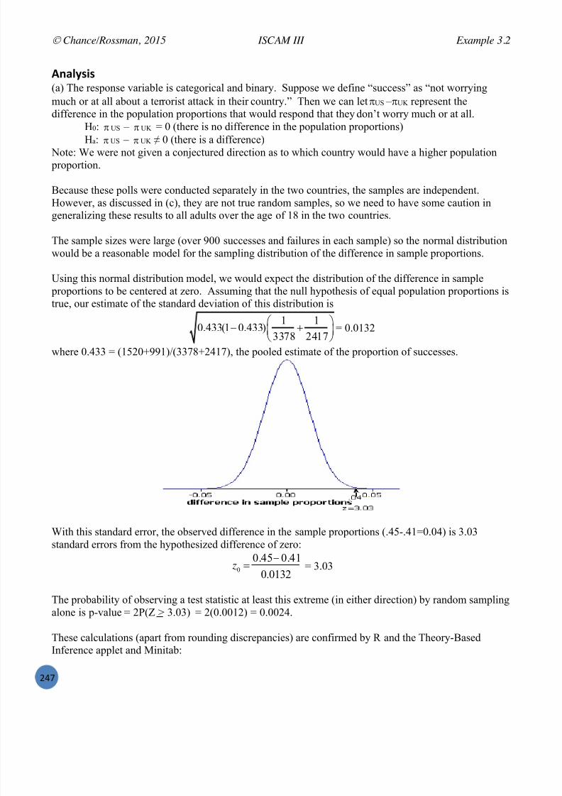
7/25/2019 Text: Investigating Statistical Concepts, Applications, and Methods
http://slidepdf.com/reader/full/text-investigating-statistical-concepts-applications-and-methods 248/428
Chance/Rossman, 2015 ISCAM III Example 3.2
!PT
<*"$6,8, (a) The res ponse variable is categorical and binary. Suppose we define “success” as “not worryingmuch or at all about a terrorist attack in their country.” Then we can let US – UK represent thedifference in the population proportions that would respond that they don’t worry much or at all.
H0: US – UK = 0 (there is no difference in the population proportions)
Ha: US – UK ≠ 0 (there is a difference) Note: We were not given a conjectured direction as to which country would have a higher population proportion.
Because these polls were conducted separately in the two countries, the samples are independent.However, as discussed in (c), they are not true random samples, so we need to have some caution ingeneralizing these results to all adults over the age of 18 in the two countries.
The sample sizes were large (over 900 successes and failures in each sample) so the normal distributionwould be a reasonable model for the sampling distribution of the difference in sample proportions.
Using this normal distribution model, we would expect the distribution of the difference in sample proportions to be centered at zero. Assuming that the null hypothesis of equal population proportions istrue, our estimate of the standard deviation of this distribution is
1 10.433(1 0.433)
3378 2417
= 0.0132
where 0.433 = (1520+991)/(3378+2417), the pooled estimate of the proportion of successes.
With this standard error, the observed difference in the sample proportions (.45-.41=0.04) is 3.03standard errors from the hypothesized difference of zero:
00.45 0.41
0.0132 z = 3.03
The probability of observing a test statistic at least this extreme (in either direction) by random samplingalone is p-value = 2P(Z > 3.03) = 2(0.0012) = 0.0024.
These calculations (apart from rounding discrepancies) are confirmed by R and the Theory-BasedInference applet and Minitab:

7/25/2019 Text: Investigating Statistical Concepts, Applications, and Methods
http://slidepdf.com/reader/full/text-investigating-statistical-concepts-applications-and-methods 249/428
Chance/Rossman, 2015 ISCAM III Example 3.2
!PU
U>C f3C8C37?C< d 7;97o3C28,: CL9;3H;A 92II;99;9 ! ,_#-Q9B084; 9?d; ! ((caQ 9B084; 83C8C37?C< !-=]_
o3C28#: CL9;3H;A 92II;99;9 ! bb,Q 9B084;9?d; ! #],cQ 9B084; 83C8C37?C< ! -=],
g244 618C76;9?9 : 8?,)8?# ! -S47;3<B7?H; 618C76;9?9: 8?,)8?# j. -d)97B7?97?I: (=-(8)HB42;: -=--#]]^
b_ X "C<G?A;<I; ?<7;3HB4 GC3 8?,)8?#:& -=-,],b]_^ Q -=-^_a-_]] *
With such a small p-value (e.g., less than 0.01), we reject the null hypothesis. If the population proportions had been equal, this tells us that there is a very small probability of random sampling aloneleading to sample proportions at least as far apart as those found by Harris. Therefore, we have strong

7/25/2019 Text: Investigating Statistical Concepts, Applications, and Methods
http://slidepdf.com/reader/full/text-investigating-statistical-concepts-applications-and-methods 250/428
Chance/Rossman, 2015 ISCAM III Example 3.2
!PV
evidence that the population proportions who worry little or not at all about terrorist attack is not thesame in the US and UK.
A 95% confidence interval for the difference in the population proportions is (0.014, 0.066). So we are95% confident that percentage of all Americans that were not worried was (in 2004) 1.4 to 6.6
percentage points higher than all Britons that were not worried about terrorist attack. This is not a largedifference in a practical sense, but we don’t believe a difference in sample proportions this large couldhave arisen by random sampling alone (in particular due to the large sample sizes).
(b) Because the sample sizes are the same but the difference in sample proportions would be smaller, the p-value for the “likelihood of attack” question would be larger. On the other hand, because the sample proportions are further apart for the “confidence in government to prevent attacks” question, the p-valuewould be even smaller. Thus, there would be more evidence that the populations of Americans andBritons differ in their opinions about government control over terrorism, but less evidence that theydiffer in their expectations for an attack.
(c) If we assume a population proportion of around 0.5, then for the US sample, the margin-of-error fora 95% confidence interval would be:
1.96 0.5(0.5) / 3378 = 0.0169.The margin-of-error for the UK sample will be a bit larger because the sample size was smaller:
1.96 0.5(0.5) / 2417 = 0.0199.If the population proportion turns out to be different from 0.5, the actual margin-of-error would besmaller. Thus, these calculations give us quick approximations to the maximal margins-of-error.
The above interpretations (p-value, confidence level, margin-of-error) rely on the samples beingrandomly selected from each population, so Harris provides a warning that their sampling method is not
by definition a probability sample. Because of this, we must have some cautions in generalizing theseresults to the larger populations (though the methods were at least similar in the two countries). Still,further investigation of Harris’ methodology (e.g., http://www.harrisinteractive.com/MethodsTools/DataCollection.aspx )reveals that they use many methods to “maintain the reliability and integrity in the sample” and the webis used as the response mechanism instead of, say, the telephone. This makes the Harris online pollmuch better than the ubi quitous “click here” non -scientific opinion polls found all over the web. Soalthough we must always worry about non-sampling errors (Investigation 1.15) with any poll, theseHarris polls can be considered as reliable as a telephone poll.

7/25/2019 Text: Investigating Statistical Concepts, Applications, and Methods
http://slidepdf.com/reader/full/text-investigating-statistical-concepts-applications-and-methods 251/428
Chance/Rossman, 2015 ISCAM III Chapter 3 Summary
!RX
).<9!/@ T 01BB<@_
In this chapter, you focused on comparing two groups on a categorical variable. You began by extendingthe simulations of sampling from a finite population to consider two independent random samples fromthe same population (same probability of success). You used a normal approximation to again findapproximate p-values and confidence intervals. You were soon cautioned against jumping to cause-and-effect conclusions when significant differences are found between the two samples. In particular,confounding variables are also a possibility with observational studies. In describing potentialconfounding variables, make sure you explain the connections to both the explanatory variable and theresponse variable, and how the confounding variable provides an alternative explanation to the observeddifference.
This led us to consider comparative experiments which utilize active imposition of the explanatoryvariable and random assignment to guard against confounding variables. In a properly designedexperiment, which may include placebos, double-blindness, and other controls, there should not be anyother substantial differences between the explanatory variable groups. Thus, if we do find a statisticallysignificant difference in the response variable, we will feel comfortable attributing that difference to theimposed explanatory variable.
Then we returned to approximating p-values through simulation, but this time modeling the randomassignment process under the null hypothesis. We “shuffled” the response s to the explanatory variablegroups, and then calculated a statistic with each shuffle to assess the null distribution of that statisticunder the null hypothesis. The hypergeometric probability distribution was seen again, this time as amathematical model for this random assignment process (leading to Fisher’s Exact Test for calculatingexact p-values). Again a normal probability model can also often be applied to approximate the p-valueand to obtain confidence intervals. Keep in mind that the normal model should be applied only withsuitably large sample sizes.
Lastly, you considered limitations to the difference in conditional probabilities as the parameter ofinterest and explored properties of relative risk and odds ratios as alternative ways to summarize theassociation between two categorical variables. In particular, with case-control studies, only the oddsratio provides a meaningful comparison. You applied your knowledge of simulation methods to obtainapproximate p-values for these statistics, learning the usefulness of transformations in normalizingdistributions. This allowed us to apply some normal-based methods for obtaining confidence intervalsfor the population relative risk and population odds ratio. Don’t forget to back -transform these intervalsto return to the original scale.

7/25/2019 Text: Investigating Statistical Concepts, Applications, and Methods
http://slidepdf.com/reader/full/text-investigating-statistical-concepts-applications-and-methods 252/428
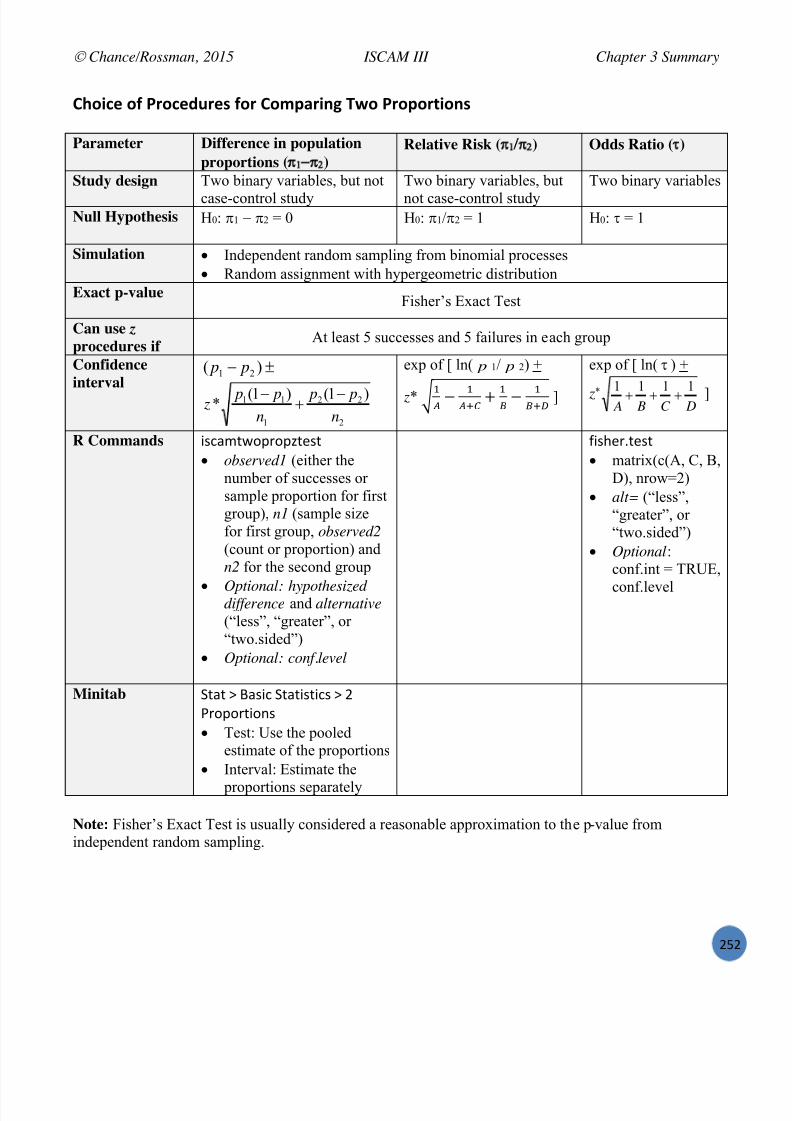
7/25/2019 Text: Investigating Statistical Concepts, Applications, and Methods
http://slidepdf.com/reader/full/text-investigating-statistical-concepts-applications-and-methods 253/428
Chance/Rossman, 2015 ISCAM III Chapter 3 Summary
!R!
)='87% '( 9:'7%54:%, (': )';?":8*> !G' 9:'?':+8'*,
Parameter Difference in populationproportions ( )
Relative Risk ( ) Odds Ratio ( )
Study design Two binary variables, but notcase-control study
Two binary variables, butnot case-control study
Two binary variables
Null Hypothesis H0: 1 2 = 0 H 0: 1/ 2 = 1 H 0: = 1
Simulation Independent random sampling from binomial processes Random assignment with hypergeometric distribution
Exact p-value Fisher’s Exact Test
Can use zprocedures if
At least 5 successes and 5 failures in each group
Confidenceinterval
)ˆˆ
( 21 p p
2
22
1
11 )ˆ
1(ˆ
)ˆ
1(ˆ
*n
p pn
p p z
exp of [ ln( pˆ
1/ pˆ
2) +
z* 1 1+ 1 1+ ]
exp of [ ln(ˆ
) +
z DC B A 1111 ]
R Commands '()&*%<18518K%,(% observed1 (either the
number of successes orsample proportion for firstgroup), n1 (sample sizefor first group, observed2 (count or proportion) andn2 for the second group
Optional: hypothesizeddifference and alternative (“less”, “greater”, or“two.sided”)
Optional: conf.level
9'(+,5/%,(% matrix(c(A, C, B,
D), nrow=2) alt= (“less”,
“greater”, or“two.sided”)
Optional :conf.int = TRUE,
conf.level
Minitab $%&% a M&(') $%&%'(%')( a !O51815%'1.( Test: Use the pooled
estimate of the proportions Interval: Estimate the
proportions separately
Note: Fisher’s Exact Test is usually considered a reasonable approximation to the p -value fromindependent random sampling.

7/25/2019 Text: Investigating Statistical Concepts, Applications, and Methods
http://slidepdf.com/reader/full/text-investigating-statistical-concepts-applications-and-methods 254/428
Chance/Rossman, 2015 ISCAM III Chapter 3 Summary
!R#
a487Q @%(%:%*7% +' M0)<B @ `':Q,?"7% L4*7+8'*, "*5 -+=%: @ )';;"*5,
9:'7%54:% 2%,8:%5 L4*7+8'* 3";% O-?+8'*,P$,% 28 %<1:<&6 %&=-, 6)&7'8")6$ 9 :6)&7'81 :,:21 .1 ;1 <=1 "7/> 9 ?1
dimnames = list(c(“row name”, “row name”),
c(“column name”, “column name”))) $,3*,.%,; =&5 35&8+ $,% 28 %<1:<&6 %&=-, &.; %+,. 2(, =&58-1%
=&58-1%F8518/%&=-,F*&%5'B.&*,7 *&53'._!G7 -,3,.; _ I7ylab = “Proportion”)
b,.,5&%, ;&%& 951* M'.1*'&- 5='.1*F.2*=,57 (&*8-, ('K,7 851=&='-'%6GN5,&%, & )1-2*. 19 # 35&8+( 8&5F*951<_)F#7WGGI<1 851815%'1. K:%,(%Y'.%,54&- '()&*%<18518K%,(%FBW7 .W7 B!7 .!7 +681%+,('K,;7
&-%,5.&%'4,7 )1.9/-,4,-G mBW )&. =, )12.% 15 851815%'1.j68,53,1*,%5') 851=&='-'%6 '()&*+68,5851=F>7 %1%&-7 (2))7 .7 -1<,5/%&'- _ Q0\$fG]15*&- &8851B'*&%'1. %1 +68,53,1*,%5') '()&*+68,5.15*F 56 86 96 (6 I[ZfYQ0\$fGb,.,5&%, ;&%& 951* +68,53,1*,%5') 5+68,5F.2*=,57 (&*8-, ('K,7 851=&='-'%6G
N5,&%, M11-,&. 915 4&-2,( =,-1< (1*, .2*=,5 5 F)5,&%'.3 &. ,*8'5')&- 8:4&-2,G (2*F;&%& g_ BGY.
Fisher’s Exact Test, confidence interval for odds ratio 9'(+,5/%,B%F*&%5'B7 &-%,5.&%'4,G
a487Q @%(%:%*7% +' B8*8+"# )';;"*5,
9:'7%54:% 2%,8:%5 B%*4$,3*,.%,; =&5 35&8+ b5&8+ a M&5 N+&5%b,.,5&%, ;&%& 951* M'.1*'&- N&-) a [&.;1* E&%& a M'.1*'&-j'(%135&* b5&8+ a j'(%135&*C,&.7 (%&.;&5; ;,4'&%'1.7 (2* 19 4&-2,( CIMa *,&. NW7 CIMa (%; NW7 CIMa (2* NW
$2**&56 (%&%'(%')( $%&% a M&(') $%&%'(%')( a E'(8-&6 E,()5'8%'4, $%&%'(%F15NUe. A;9I3?L; I, G
L4,5-&6 .15*&- )254, 1. +'(%135&* ['3+% )-')>7 0;; a E'(%5'=2%'1. Q'%]15*&- O51=&='-'%6 O-1% b5&8+ a O51=&='-'%6 O-1%I<1 851815%'1. K:%,(%Y'.%,54&- $%&% a M&(') $%&%'(%')( a ! O51815%'1.(
Use “not equal to” &-%,5.&%'4, 915 )1.9';,.), '.%,54&-j68,53,1*,%5') 851=&='-'%6 b5&8+ a O51=&='-'%6 E'(%5'=2%'1. O-1%b,.,5&%, ;&%& 951* +68,53,1*,%5') N&-) a [&.;1* E&%& a j68,53,1*,%5')N5,&%, M11-,&. 915 4&-2,( =,-1< (1*, .2*=,5 5 F)5,&%'.3 &. ,*8'5')&- 8:4&-2,G
N&-) a N&-)2-&%157 ,B85,(('1.? (2*F)T g_ BGY.CIMa -,% )WX _ F)T g_ BGCIMa -,% >W _ (2*FWXGY.
CIMa 85'.% >WFisher’s Exact Test $%&% a M&(') $%&%'(%')( a ! O51815%'1.(
7/25/2019 Text: Investigating Statistical Concepts, Applications, and Methods
http://slidepdf.com/reader/full/text-investigating-statistical-concepts-applications-and-methods 255/428
Chance/Rossman, 2015 ISCAM III Chapter 4
!RP
CHAPTER 4: COMPARISONS WITH QUANTITATIVE VARIABLES
This chapter parallels the previous one in many ways. We will continue to consider studies where thegoal is to compare a response variable between two groups. The difference here is that these studies willinvolve a quantitative response variable rather than a categorical one. The methods that we employ to
analyze these data will therefore be different, but you will find that the basic concepts and principles thatyou learned in Chapters 1 3 still apply. These include the principle of starting with numerical andgraphical summaries to explore the data, the concept of statistical significance in determining whetherthe difference in the distribution of the response variable between the two groups is larger than wewould reasonably expect from randomness alone, and the importance of considering how the data werecollected in determining the scope of conclusions that can be drawn from the study.
Section 1: Comparing groups – Quantitative responseInvestigation 4.1: Employment discrimination?
Section 2: Comparing two population means
Investigation 4.2: NBA Salaries – Independent random samples, t proceduresInvestigation 4.3: Left-handedness and life expectancy – Factors influencing significance
Section 3: Comparing for two treatment meansInvestigation 4.4: Lingering effects of sleep deprivation – Randomization testsInvestigation 4.5: Lingering effects of sleep deprivation (cont.) – Two-sample t -testsInvestigation 4.6: Ice cream serving sizes – Two-sample t -confidence intervalInvestigation 4.7: Cloud seeding – Strategies for non-normal data
Section 4: Matched Pairs DesignsInvestigation 4.8: Chip melting times – Independent vs. paired design, technology
Investigation 4.9: Chip melting times (cont.) – Inference (simulation, paired t -test)Investigation 4.10: Comparison shopping – ApplicationInvestigation 4.11: Smoke alarms – McNemar’s test (paired categorical d ata)
Example 4.1: Age Discrimination? – Randomization testExample 4.2: Speed Limit Changes – Two-sample t -proceduresExample 4.3: Distracted Driving? (cont.) – Paired t -procedures

7/25/2019 Text: Investigating Statistical Concepts, Applications, and Methods
http://slidepdf.com/reader/full/text-investigating-statistical-concepts-applications-and-methods 256/428
Chance/Rossman, 2015 ISCAM III Investigation 4.1
!RR
SECTION 1: COMPARING GROUPS – QUANTITATIVE REPONSE
@. %+'( )+&8%,57 <, <'-- 91)2( 1. )1*8&5'.3 %<1 35128( 1. & A2&.%'%&%'4, 5,(81.(, 4&5'&=-,/ 03&'.7 %+, 5,&(1.'.3'( (%'-- %+, (&*, &( '. N+/ W – #7 =2% <, <'-- (,, (1*, (*&-- )+&.3,( '. %+, ;,%&'-(/ J, (%&5% <'%+ & (*&--'.4,(%'3&%'1. %1 5,4',< >,6 ';,&( &.; %+,. <, 8&5&--,- N+&8%,5 # '. 9'5(% )1.(';,5'.3 5&.;1* (&*8-'.3 &.; %+,.5&.;1* &(('3.*,.%7 =1%+ 915 ()18, 19 )1.)-2('1.( =2% &-(1 915 +1< <, <'-- ;,('3. 125 ('*2-&%'1./
Investigation 4.1: Employment Discrimination?
Robert Martin turned 55 in 1991. Earlier in that same year, the Westvaco Corporation, which makes paper products, decided to downsize. They ended up laying off roughly half of the 50 employees in theengineering department where Martin worked, including Martin. Later that year, Martin went to court,claiming that he had been fired because of his age. A major piece of evidence in Martin’s case was
based on a statistical analysis of the relationship between the ages of the workers and whether they losttheir jobs.
Part of the data analysis presented at his trial concerned the ten hourly workers who were at risk oflayoff in the second of five rounds of reductions. At the beginning of Round 2 of the layoffs, there wereten employees in this group. Their ages were 25, 33, 35, 38, 48, 53, 55, 55, 56, 64. Three were chosenfor layoff: the two 55-year-olds (including Martin) and the 64-year old.
(a) Create stacked dotplots of the ages of the employees who were retained and laid off.
retained
laid offDo these data seem to support the claim that the laid-off employees tended to be older than those whowere not laid off?
(b) One way to measure this support is to compare the difference in the average ages of the two groups.Calculate the mean age of the employees that were laid off and the mean age of the employees that werenot laid off ( )
retained off laid x x .
(c) Although we see some evidence of an age difference, on average, between these two groups, it’s still possible that the employers just randomly decided which three employees to layoff. How would youexpect the behavior of these dotplots to compare if the layoff decisions had been made completely atrandom?

7/25/2019 Text: Investigating Statistical Concepts, Applications, and Methods
http://slidepdf.com/reader/full/text-investigating-statistical-concepts-applications-and-methods 257/428
Chance/Rossman, 2015 ISCAM III Investigation 4.1
!RS
(d) Describe how you could generate one “could have been” observation under this assumption that thelay-off decisions are made completely at random.
(e) If we consider the outcomes where three of the ten employees are laid off, how many of theseoutcomes are “as extreme” as the observed result? How many are “more extreme”? [ Hint : List the agesof the three employees that are laid off for these results.]
(f) How many different ways are there to form these two groups, three to be laid off and seven retained,if the decisions are made completely at random?
(g) How many of these random splits have three of the four oldest people in the laid-off group?
The dotplot below shows all possible values for the “difference in mean age” for the laid -off groupminus the retained group for all possible splits into 3 laid-off employees and 7 retained.
(h) What is the approximate average of this distribution? Is this what you expected?
(i) Is this distribution symmetric? Why or why not?
Discussion: Although we might suspect the distribution to be centered at zero, the graph is not expectedto be symmetric because the group sizes are unequal and we subtracted laid-off – retained. Also, thedata set is small so there will be “granularity” between the possible values for the difference.
(j) Which of the outcomes in the dotplot correspond to the outcomes you listed in (g)? [ Hint : Find thedifference in group means when the following ages are assigned to the laid-off group.]
55, 55, 56: 55, 55, 64:
55, 56, 64: 53, 56, 64:

7/25/2019 Text: Investigating Statistical Concepts, Applications, and Methods
http://slidepdf.com/reader/full/text-investigating-statistical-concepts-applications-and-methods 258/428
Chance/Rossman, 2015 ISCAM III Investigation 4.1
!RT
(k) Use your result from (f) and (g) to calculate an exact p-value for the null hypothesis that the lay-offdecisions were made completely at random. How can you interpret this p-value? [ Hint : How wasrandomness used in the study?]
(l) What do you conclude from the p-value you calculated in (k)? [ Hint : Think about the significance ofthe result and the type of study.]
(m) Remind the lawyers what limitations there are to the conclusions that can be made in this study.
0+456 )'*7$4,8'*,In this analysis, you assumed a null model – the lay-offs are made completely at random – and youconsidered all 120 possible assignments of 7 people to be retained and 3 people to be laid off. (Youcould have flipped a coin for each employee, but that would lay off 50% in the long-run rather thanfixing 3 to be laid off.) Of these 120 possible assignments, we want to know how many are “at least as extreme” as the observed result. If we focus on the outcomes where 3 of the 4 oldest people end up inthe laid-off group, only the 55, 56, 64 combination has a difference in means (17.33 years) larger thanwhat we observed (16.86, which can happen two ways). The 55, 55, 56 combination has a smallerdifference in means (13.04) and the 53, 56, 64 combination also does not quite have as large a differencein means (16.38). So the exact p-value = 3/120 = 0.025, which tells us that if these decisions had been
made completely at random, there is a 2.5% chance we would see a combination of ages at least asextreme as the actual outcome as measured by the difference in group means. This is moderate evidencethat the decision making process was not at random. If you do find this evidence compelling, you mustkeep in mind the observational nature of the data; we cannot draw any cause-and-effect conclusionsabout the reasons for the non-random lay-off decisions.
The reasoning process of statistical significance remains the same – how often would random chancegive me a result at least as extreme? We will still need to consider how we want to measure the groupdifferences (e.g., choice of statistic) and how we can approximate the p-value (e.g., by modelling thehypothetical randomness assumed by the null hypothesis), especially when a listing of all possibleoutcomes is not feasible. Large sample sizes will also again allow us to use a convenient confidence
interval formula. Once you have a p-value or confidence interval, you interpret them in the same way asin previous chapters, while also considering the limitations of the study design.
9:"7+87% 9:'#$%; UDH(a) Suppose the following individuals were laid off: 25, 35, 38. What would be the difference in themean age of those who were laid off and those who were retained?(b) What would be the exact p-value for this difference in means from part (a) if the alternativehypothesis was that there was a bias against the younger employees?

7/25/2019 Text: Investigating Statistical Concepts, Applications, and Methods
http://slidepdf.com/reader/full/text-investigating-statistical-concepts-applications-and-methods 259/428
Chance/Rossman, 2015 ISCAM III Investigation 4.2
!RU
SECTION 2: COMPARING TWO POPULATION MEANS
In this section, we want to focus on quantitative data arising from two independent random samples.We will first begin with a hypothetical situation to explore how our statistic should behave under certainassumptions about the populations. We will then discuss a theoretical result justifying use of a t- distribution for the reference distribution in finding p-values and confidence intervals.
Investigation 4.2: NBA SalariesThe file ]M0$&-&5',(!XWP/%B% contains season salaries (in millions of dollars) for all NBA basketball
players at the start of the 2014-15 season (posted Oct 16, 2014; downloaded from BallnRoll , July 2015).Players without a team affiliation or without a listed salary were not included in the data set.
(a) Do you expect salary data to be symmetric or skewed, and if skewed, in which direction? Explain.
(b) Which do you suspect will be larger, the mean or median salary? Explain.
2%,7:8?+8F% 0+"+8,+87,When using graphs to compare groups it is especially important that comparative graphs be drawn onthe same scale.
!%7=*'$'>6 2%+'4: – )';?":"+8F% N:"?=,
M* 2%,7:8?+8F% 0+"+8,+87, "??$%+ Copy the (&-&56 and )1.9,5,.), data to the clipboard. In the applet, check the Stacked box and confirmthe ordering of the category and quantitative variables. Paste the data into the Sample data window and
press Use Data . You have radio button options for Histograms and Boxplots.
M* @a ?9IB0AC784C7&7?0;Q 1;B3* @.82% A2&.%'%&%'4, %+,. )&%,315')&- 4&5'&=a 6?97CD3B0&p9B4B31q IC<G;3;<I;Q [,*,*=,5 %1 -1&; -&%%'), 8&)>&3,n 4B1C27 ! I&,Q#*Q <?<7!#-* N5,&%,( 4,5%')&- -&612%7 .2*=,5 19 ='.(a ?9IB0LC[84C7&9B4B31Q IC<G;3;<I;* L[a LC[84C7&9B4B31pIC<G;3;<I;Q 6C3?d!UPJ'Q 14BL!59B4B31 &0?4 W*5*

7/25/2019 Text: Investigating Statistical Concepts, Applications, and Methods
http://slidepdf.com/reader/full/text-investigating-statistical-concepts-applications-and-methods 260/428
Chance/Rossman, 2015 ISCAM III Investigation 4.2
!RV
M* B8*8+"# Choose Graph > Dotplot . Select One Y, With Groups option. Press OK . Specify quantitative variable in Graph variables box
and then click inside the Categorical variables boxand specify categorical variable.
Press OK .
Choose Graph > Histogram . Select Simple . Specify the quantitative variable in
the Graph variables box. Select Multiple Graphs . Select the By variables tab. Specify the categorical variable in the “separate
panels” box. Press OK twice. Optional : You can right click on Graph, select
Panel.., then Arrangement, setting 2 rows and 1column.
Choose Graph > Boxplot . Specify One Y, With Groups , press OK . Enter the quantitative variable in the Graph variables
box and then click in the Categorical variables boxand enter the categorical variable.
Press Scale and check the Transpose value andcategory scales box. FC&>,( +15'K1.%&-G
Press OK twice.
And we can easily calculate separate summary statistics for the two conferences:
!%7=*'$'>6 2%+'4: – 34;%:87"$ 04;;":8%,
M* @To get separate descriptive statistics for each group:. ?9IB09200B31&9B4B31Q IC<G;3;<I;*
Note: This adds the second (explanatory) variable. You still have the option of entering “digits = ” tospecify the number of significant digits you want displayed.
M* B8*8+"# Choose Stat > Basic Statistics > Display Descriptive Statistics . Specify the quantitative variable in the Variables box and then click in the By variables box and
specify the categorical variable. Optional : Under Statistics you can choose which numbers are calculated.

7/25/2019 Text: Investigating Statistical Concepts, Applications, and Methods
http://slidepdf.com/reader/full/text-investigating-statistical-concepts-applications-and-methods 261/428
Chance/Rossman, 2015 ISCAM III Investigation 4.2
!SX
(c) Create a comparative graph and calculate the difference in the population mean salaries between theEastern Conference and the Western Conference. (Notice that because the dataset lists salaries for all
players in the NBA, you are working with a population and not a sample.) What symbols should you useto reference to this difference?
(d) Also determine the population sizes and the population standard deviations and record these below,using appropriate symbols.
(e) Suppose we weren’t able to perform a census and only had resources to find the salaries for 40 players. How would you select the 40 players?
(f) Use technology to select a random sample of 20 players from each league:
!%7=*'$'>6 2%+'4: – 0%$%7+8*> M*5%?%*5%*+ @"*5'; 0";?$%,
M* @ %&>, & 5&.;1* (&*8-, 951* ,&)+ ;'4'('1.. >;979B084; ! 9B084;&9B4B31i>6?I6&IC<G;3;<I; !! 5>;97;3<5*kQ #-*. ;B979B084; ! 9B084;&9B4B31i>6?I6&IC<G;3;<I; !! 5;B97;3<5*kQ #-*. 9B4B31=9B084; ! AB7B=G3B0;&>;979B084;Q ;B979B084;*. <B0;9&9B4B31=9B084;* ! I&5>;97;3<5Q 5;B97;3<5*
M* B8*8+"#NUe. 2<97BI@ I_ I^ IcO (8-'% %+, %<1 )1.9,5,.),( '.%1 %<1 )1-2*.(KJe". 92L9 I]=NUe. 9B084; #- I^ Ia %&>, & 5&.;1* (&*8-, 951* ,&)+ )1-2*. NUe. 9B084; #- Ic Ib NUe. <B0; Ia n;B97 9B084;n Ib n>;97 9B084;n
(g) Create comparative graphs and descriptive statistics for these sample data. [Note: Your data iscurrently “unstacked” which requires a different approach than “stacked data” in most software.]
!%7=*'$'>6 2%+'4: – 1*,+"7Q%5 5"+"
M* @ +&4, %1 9'5(% (%&)> %+, ;&%& . K7BI@;A%B7B ! 97BI@&9B4B31=9B084;iQ I&5>;97;3<5Q5;B97;3<5*k*. <B0;9&K7BI@;A%B7B* ! I&59B4B315Q 5A?H?9?C<5*. ?9IB0AC784C7&K7BI@;A%B7BW9B4B31Q K7BI@;A%B7BWA?H?9?C<*. ?9IB09200B31&K7BI@;A%B7BW9B4B31Q K7BI@;A%B7BWA?H?9?C<*

7/25/2019 Text: Investigating Statistical Concepts, Applications, and Methods
http://slidepdf.com/reader/full/text-investigating-statistical-concepts-applications-and-methods 262/428
Chance/Rossman, 2015 ISCAM III Investigation 4.2
!SW
M* B8*8+"# Select Graph > Dotplot , and then Multiple Y’s, Simple option, press OK. Specify the East sample and West sample columns in the Graph variables box and press OK. Double click on the Data axis label and in the Text box enter a better axis label. Select Stat > Basic Statistics > Descriptive Statistics and enter both variables in the Graph
variables box.
Record the sample means and sample standard deviations for your samples. How do the sample resultscompare to the population results? What about the shapes of the samples?
(h) Calculate your difference in means and pool with the rest of your class.
(i) How would you describe the shape of this distribution? Is this what you expected?
(j) What is the approximate center of this distribution? Is this what you expected?
(k) But of course, what you really want to know about is the variability. Is there more or less variabilityin this distribution compared to the variability in each population (part (d))?
(l) We know there should be less variability because we are talking about sample means rather thanindividual observations. But how much variability do we expect to find in the distribution of samplemeans taken from the Western conference? What about the Eastern conference? Is the variability in the
difference in sample means larger or smaller than in the individual distributions?
(m) To confirm these observations, we need to take a lot more samples. Outline the simulation steps weneed to use.

7/25/2019 Text: Investigating Statistical Concepts, Applications, and Methods
http://slidepdf.com/reader/full/text-investigating-statistical-concepts-applications-and-methods 263/428
Chance/Rossman, 2015 ISCAM III Investigation 4.2
!S!
(n) Use a premade script or macro to carry out the simulation: M* @I Run the ]M0$&-&56$&*8-,(/[ script to generate 1000 repetitions. M* B8*8+"#: Use the ]M0$&-&56$&*8-,(/*%= or ]M0$&-&56$&*8-,(/*&) macro to generate 1000
repetitions. (For the latter, remember to save the macro and the data file in the same folder.)
Calculate the difference in sample means for each repetition. Examine and describe the distribution ofthe differences of sample means. [ Hint : Reconsider questions (i), (j), and (k).]
Key Result: A theorem similar to the Central Limit Theorem indicates that if we have two infinite,normally distributed populations, with means 1 and 2 and standard deviations 1 and 2, and we take
independent random samples from each population, the sampling distribution of 21 X X will follow a
normal distribution with mean 1 – 2 and standard deviation2
22
1
21
nn .
This is a nice theoretical result, but we seldom meet these conditions exactly.
(o) Identify two characteristics of our populations that do not agree with this statement.
A third, but perhaps the biggest, issue is that the population standard deviations are unknown.
(p) Suggest a formula for estimating the standard deviation of the difference in sample means.
So then what we really need to know about is the distribution of
2
22
1
21
2121 )()(
n
S
n
S
X X .
(q) Create this statistic for each repetition of your earlier simulation results and then examine thedistribution of this statistic. Is it approximately normal? Where is it centered?

7/25/2019 Text: Investigating Statistical Concepts, Applications, and Methods
http://slidepdf.com/reader/full/text-investigating-statistical-concepts-applications-and-methods 264/428
Chance/Rossman, 2015 ISCAM III Investigation 4.2
!S#
Discussion: The sample sizes of 20 for each group appear to be large enough for a t -distribution (even anormal distribution) to reasonably approximate the distribution of this statistic. If the populationdistributions had themselves been normally distributed (and large), then a t -distribution will be a goodapproximation of the statistic for any sample sizes. The more skewed the population shapes, the largerthe sample sizes need to be for you to safely use the t -distribution. Notice even with these very skewed
populations, because their shapes and sample sizes were similar, we didn’t need very large sample sizesat all for the standardized statistic to follow a t distribution. One remaining question is what to use forthe degrees of freedom for the t -distribution. In the one-sample case we used n – 1. For two samples,it’s actually more complicated. There is a “Welch -Satterwaite” approximation that involves the samplesizes and the unknown population standard deviations, though it doesn’t always result in integer values.We will leave this calculation up to technology. You only need to realize that the degrees of freedom arerelated to the sample sizes and as the sample sizes becomes large, the t-distribution loses more and moreof the heaviness in the tails and approaches the (standard) normal distribution. If you need to determinea p-value or critical value “by hand,” we suggest using the following simple approximation for thedegrees of freedom: min (n1 – 1, n2 – 1), the smaller of the two sample sizes minus one.
In this case, we could use 19 as the approximate degreesof freedom. Notice that this sample size is large enoughthat the t-distribution looks a lot like the normaldistribution as well, which should agree with yourobservation in (q). But we will continue to use the t-distribution rather than the normal distribution to stillaccount for additional variation from our estimates of the
population standard deviations.
Especially when the population shapes are similar and thesample sizes are similar, the t-distribution provides a
pretty good approximation to the sampling distribution of21 X X , even for non-normal populations.
04;;":6 '( +G'\,";?$% " ?:'7%54:%,
Parameter: = the difference in the population means
To test H 0: = 0
Test statistic:
2
22
1
21
0210
)(
ns
ns
x xt
t -Confidence interval for
)( 21 x x + t * 2
22
1
21
n
s
n
s
Approximate degrees of freedom:Compare this to a t-distribution with
degrees of freedom equal to the smaller ofthe two samples sizes minus one:min(n 1, n2) – 1.
Technical conditions: These procedures are considered valid if the sample distributions arereasonably symmetric or the sample sizes are both at least 20.
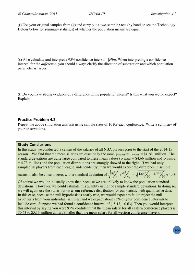
7/25/2019 Text: Investigating Statistical Concepts, Applications, and Methods
http://slidepdf.com/reader/full/text-investigating-statistical-concepts-applications-and-methods 265/428
Chance/Rossman, 2015 ISCAM III Investigation 4.2
!SP
(r) Use your original samples from (g) and carry out a two-sample t -test (by hand or see the TechnologyDetour below for summary statistics) of whether the population means are equal.
(s) Also calculate and interpret a 95% confidence interval. [ Hint : When interpreting a confidenceinterval for the difference , you should always clarify the direction of subtraction and which population
parameter is larger.]
(t) Do you have strong evidence of a difference in the population means? Is this what you would expect?Explain.
9:"7+87% 9:'#$%; UDRRepeat the above simulation analysis using sample sizes of 10 for each conference. Write a summary ofyour observations.
0+456 )'*7$4,8'*,In this study we conducted a census of the salaries of all NBA players prior to the start of the 2014-15season. We find that the mean salaries are essentially the same, eastern = western = $4.261 million. Thestandard deviations are quite large compared to these mean values ( eastern = $4.66 million and western = 4.73 million) and the population distributions are strongly skewed to the right. If we had onlysampled 20 players from each league, independently, then we would expect the difference in sample
means to also be close to zero, with a standard deviation of2
22
1
21
nn = 20
73.420
66.4 22 1.48.
Of course we wouldn’t usually know that, because we are unlikely to know the population standarddeviations. However, we could estimate this quantity using the sample standard deviations. In doing so,
we will again use the t distribution as our reference distribution for our statistic with quantitative data.In this case, because the null hypothesis is nearly true, we would expect to fail to reject the nullhypothesis from your individual samples, and we expect about 95% of your confidence intervals toinclude zero. Suppose we had found a confidence interval of ( 5.13, 0.63). Then you would interpretthis interval by saying you were 95% confident that the mean salary for all eastern conference players is$0.63 to $5.13 million dollars smaller than the mean salary for all western conference players.

7/25/2019 Text: Investigating Statistical Concepts, Applications, and Methods
http://slidepdf.com/reader/full/text-investigating-statistical-concepts-applications-and-methods 266/428
Chance/Rossman, 2015 ISCAM III Investigation 4.2
!SR
1,8*> !%7=*'$'>6 +' )"::6 '4+ +=% !G'\0";?$% " \!%,+,
In using technolo gy, you need to consider how the data are available: Do you have the “raw data”(meaning all the individual data values) or just the summary statistics (sample sizes, means, SDs)? Mostsoftware packages will assume raw data is “stacked” – each column represents a different variable (all
response variable values in one column, the explanatory variable in a second column). Also notice that being able to run the t -test with only the summary data is one advantage the t -test has over thesimulation. But also keep in mind that the t -output is valid only when the population distributions arenormal or the sample sizes are large. When reporting your results, make sure you specify whichtechnology you used, as different software use different degrees of freedom. You will also need to watchfor the direction of subtraction that the software uses automatically (often alphabetical by group name).
There is also a version of the two-sample t -test that makes an additional assumption – the populationstandard deviations are equal. The standardized statistic has the following form:
21
210
/1/1 nns
x xt
p where
2)1()1(
21
222
211
nnsnsn
s p , a pooled estimate of the common SD.
This “ pooled t -test” has some advantages (namely higher power), when the population standarddeviations are equal. However, this additional condition can be difficult to assess from your sample data.The benefits do not appear to outweigh the risks of applying this assumption whe n you shouldn’t. So inthis text we will focus on “unpooled t -tests” only.
!%7=*'$'>6 2%+'4: !G'\0";?$% " \!%,+ O4*?''$%5b ,4;;":6 5"+"P
M* @ The '()&*%<1(&*8-,% function takes the following inputs:C Group 1 mean, standard deviation, sample size (in that order) C Group 2 mean, standard deviation, sample size (in that order)
C Optional: hypothesized difference (default is zero)C Optional: alternative (“less”, “greater”, or “two.sided”) C Optional: conf.level
For example: ?9IB07>C9B084;7&[,!c_Q 9A,!,_Q <,!aaaQ [#!^^Q 9A#!,_Q <#!bbQ B47!5D3;B7;35*
M* B8*8+"# Choose Stat > Basic Statistics > 2-Sample t . Use the pull0down menu to select Summarized
data . Enter the summary statistics. Press Options and specify direction of Alternative. Press OK twice.
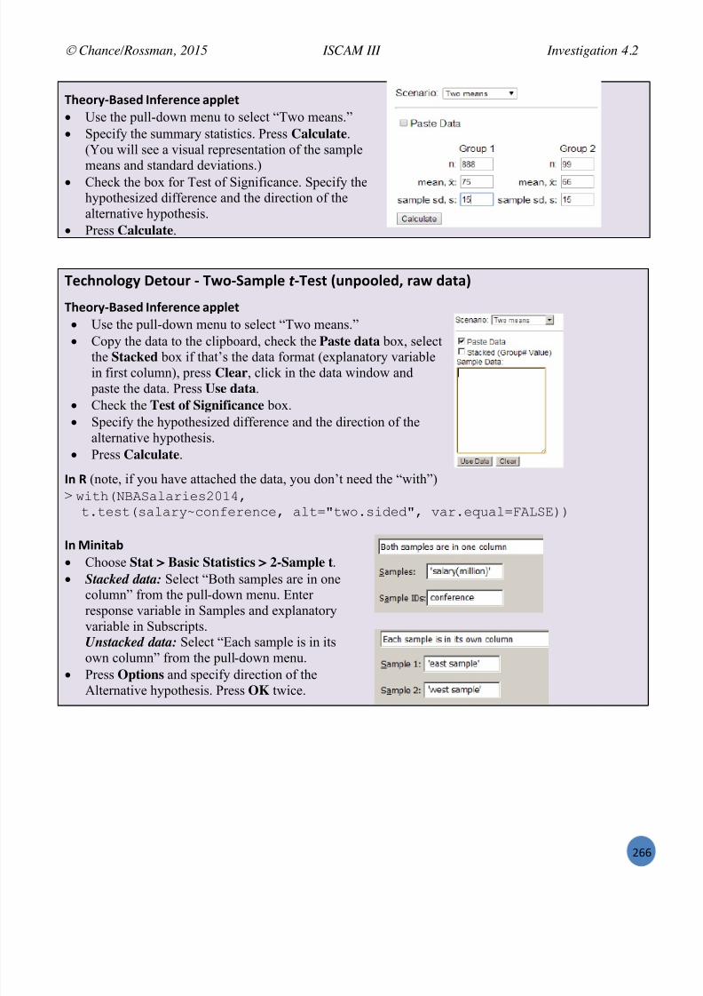
7/25/2019 Text: Investigating Statistical Concepts, Applications, and Methods
http://slidepdf.com/reader/full/text-investigating-statistical-concepts-applications-and-methods 267/428
Chance/Rossman, 2015 ISCAM III Investigation 4.2
!SS
!=%':6\C",%5 M*(%:%*7% "??$%+ Use the pull- down menu to select “Two means.” Specify the summary statistics. Press Calculate .
(You will see a visual representation of the samplemeans and standard deviations.)
Check the box for Test of Significance. Specify thehypothesized difference and the direction of thealternative hypothesis.
Press Calculate .
!%7=*'$'>6 2%+'4: \ !G'\0";?$% " \!%,+ O4*?''$%5b :"G 5"+"P
!=%':6\C",%5 M*(%:%*7% "??$%+ Use the pull- down menu to select “Two means.” Copy the data to the clipboard, check the Paste data box, select
the Stacked box if that’s the data format (explanatory variablein first column), press Clear , click in the data window and
paste the data. Press Use data . Check the Test of Significance box. Specify the hypothesized difference and the direction of the
alternative hypothesis. Press Calculate .
M* @ (note, if you have attached the data, you don’t need the “with”) > >?76&geSKB4B3?;9#-,]Q
7=7;97&9B4B31pIC<G;3;<I;Q B47!57>C=9?A;A5Q HB3=;\2B4!RSEK'**
M* B8*8+"# Choose Stat > Basic Statistics > 2-Sample t . Stacked data: Select “Both samples are in one
column” from the pull -down menu. Enterresponse variable in Samples and explanatoryvariable in Subscripts.Unstacked data: Select “Each sample is in itsown column” from the pull -down menu.
Press Options and specify direction of theAlternative hypothesis. Press OK twice.
7/25/2019 Text: Investigating Statistical Concepts, Applications, and Methods
http://slidepdf.com/reader/full/text-investigating-statistical-concepts-applications-and-methods 268/428
Chance/Rossman, 2015 ISCAM III Investigation 4.3
!ST
Investigation 4.3: Left-Handedness and Life Expectancy
Psychologist Stanley Coren has conducted several studies investigating the life expectancy of left-handers compared to right-handers, believing that the stress of being left-handed in a right-handed worldleads to earlier deaths among the left-handers. In one study Coren and Halpern (1991) sent surveys to
thousands of next-of-kin of recently deceased southern Californians and asked whether the person had been right-handed or left-handed. They were very careful in how they collected their data. First, theyconsulted a bereavement counselor who suggested that they not contact anyone unless at least 9 monthshad passed since the death. The counselor also suggested that they make the contact as gentle as possibleand not follow up or press people for responses. The researchers also decided that they would notcontact next of kin if the death had been a result of murder or suicide or if the deceased was a child age6 or younger. They received 987 replies and found that the average age of right-handed people at deathwas 75 years and for left-handed people it was 66 years.
(a) Is this an observational study or an experiment?
(b) Did the researchers take a random sample of left-handers and an independent random sample ofright-handers? Is it reasonable to consider these samples independent?
Even though the researchers did not take a random sample of left-handers and a separate random sampleof right-handers, we are still willing to consider these samples as independent because the results for onegroup should have no effect on the results for the other group. In a situation with two independentrandom samples, we can apply the two-sample t -test to make inferences about the difference in the
population means.
(c) The summary of the study reported the sample means; what additional information do we need toassess the statistical significance of their difference? Why is this information important?
(d) Let L represent the mean lifetime for the population of left-handers and let R represent the meanlifetime for the population of right-handers. State the null and alternative hypotheses for Coren andHalpern’s study (based on the research conjecture).
The table below lists some guesses for the sample size breakdown (based on estimates of the proportionof the population that are left-handed) and the sample standard deviations.
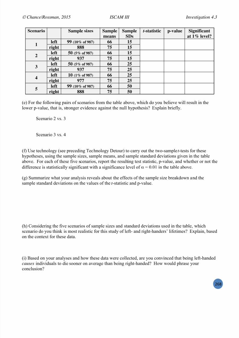
7/25/2019 Text: Investigating Statistical Concepts, Applications, and Methods
http://slidepdf.com/reader/full/text-investigating-statistical-concepts-applications-and-methods 269/428

7/25/2019 Text: Investigating Statistical Concepts, Applications, and Methods
http://slidepdf.com/reader/full/text-investigating-statistical-concepts-applications-and-methods 270/428
Chance/Rossman, 2015 ISCAM III Investigation 4.3
!SV
(j) Part of the motivation for this research was an earlier study by Porac and Coren (1981) that surveyed5147 men and women of all ages in North America. They found that 15% of ten-year-olds were left-handed, compared to only 5% of fifty-year-olds and less than 1% of eighty-year-olds. At the age of 85,right-handers outnumbered left-handers by a margin of 200 to 1. Suggest another explanation for these
puzzling findings that actually provides a counter-argument to the conclusion from the 1991 Coren and
Halpern study that left-handers tend to live shorter lives than right-handers.
0+456 )'*7$4,8'*, The difference in the sample mean lifetimes does appear to be statistically significant for all
reasonable choices of the sample sizes and the sample standard deviations, so we have strong evidencethat left-handers do tend to have shorter life spans than right-handers. However, there are numerouscautions to heed when drawing conclusions from such a study. This was a retrospective study withvoluntary response, and in fact the researchers reported that they tended to hear from the left-handedrelatives more often than right-handers, and they only heard from fewer than half of the familiescontacted. There is also no information given about the proportion of left-handers in the two southernCalifornia counties studied or the average ages of their residents now. In particular, one explanation forthe lower percentage of left-handers among the elderly is not that they have died younger but that it used
to be quite common practice to strongly encourage left-handed children to switch to being right-handed. Nowadays, that is less common (in fact many athletes love having this advantage!), and so there is ahigher percentage of left-handers among younger age groups. This helps to explain why the left-handerswho had died would tend to be younger. In other words, maybe the average age difference betweenliving left-handers and right-handers is also nine years.
These studies have actually become hot topics for debate as some other studies have not been able toreplicate Coren and Halpren’s results. Other prosp ective longitudinal studies in the United States(Marks and Williams, 1991; Wolf, D’Agostino, and Cobb, 1991) have not found a significant differencein age at death. Still others have found connections between handedness and accident rates, lower birthr ates, cancer, alcohol misuse, smoking, and schizophrenia. Alas, we don’t see any randomized,comparative experiments being conducted to answer these questions in the near future!
Discussion : You should have found that larger variability in each sample (so a larger SE) produces alarger p-value and therefore less convincing evidence that the population means differ. Or to put this ina more positive light: Reducing variability within groups makes it easier to distinguish between thegroups. You should also have found that a bigger discrepancy in sample sizes between the two groups
produces a larger p-value and therefore less convincing evidence that the population means differ.
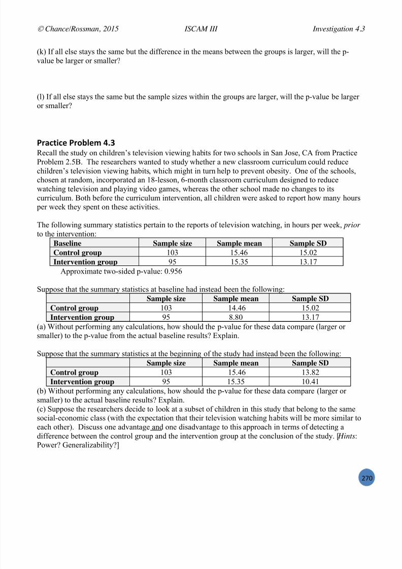
7/25/2019 Text: Investigating Statistical Concepts, Applications, and Methods
http://slidepdf.com/reader/full/text-investigating-statistical-concepts-applications-and-methods 271/428
Chance/Rossman, 2015 ISCAM III Investigation 4.3
!TX
(k) If all else stays the same but the difference in the means between the groups is larger, will the p-value be larger or smaller?
(l) If all else stays the same but the sample sizes within the groups are larger, will the p-value be largeror smaller?
9:"7+87% 9:'#$%; UDTRecall the study on children’s television viewing hab its for two schools in San Jose, CA from PracticeProblem 2.5B. The researchers wanted to study whether a new classroom curriculum could reducechildren’s television viewing habits, which might in turn help to prevent obesity. One of the schools,chosen at random, incorporated an 18-lesson, 6-month classroom curriculum designed to reducewatching television and playing video games, whereas the other school made no changes to its
curriculum. Both before the curriculum intervention, all children were asked to report how many hours per week they spent on these activities.
The following summary statistics pertain to the reports of television watching, in hours per week, prior to the intervention:
Baseline Sample size Sample mean Sample SDControl group 103 15.46 15.02Intervention group 95 15.35 13.17
Approximate two-sided p-value: 0.956
Suppose that the summary statistics at baseline had instead been the following:
Sample size Sample mean Sample SDControl group 103 14.46 15.02Intervention group 95 8.80 13.17
(a) Without performing any calculations, how should the p-value for these data compare (larger orsmaller) to the p-value from the actual baseline results? Explain.
Suppose that the summary statistics at the beginning of the study had instead been the following:Sample size Sample mean Sample SD
Control group 103 15.46 13.82Intervention group 95 15.35 10.41
(b) Without performing any calculations, how should the p-value for these data compare (larger orsmaller) to the actual baseline results? Explain.(c) Suppose the researchers decide to look at a subset of children in this study that belong to the samesocial-economic class (with the expectation that their television watching habits will be more similar toeach other). Discuss one advantage and one disadvantage to this approach in terms of detecting adifference between the control group and the intervention group at the conclusion of the study. [ Hints :Power? Generalizability?]

7/25/2019 Text: Investigating Statistical Concepts, Applications, and Methods
http://slidepdf.com/reader/full/text-investigating-statistical-concepts-applications-and-methods 272/428
Chance/Rossman, 2015 ISCAM III Investigation 4.4
!TW
SECTION 3: COMPARING TWO TREATMENT MEANS
I+, 85,4'12( (,)%'1. 91)2(,; 1. A2&.%'%&%'4, ;&%& &5'('.3 951* %<1 '.;,8,.;,.% 5&.;1* (&*8-,(/ I+'( (,)%'1.<'-- 91)2( 1. A2&.%'%&%'4, ;&%& &5'('.3 951* 5&.;1*'K,; ,B8,5'*,.%(/ J, <'-- &3&'. )1.(';,5 ('*2-&%'1.:=&(,;7,B&)%7 &.; %+,156:=&(,; 8:4&-2,(7 &( <,-- &( <+&% &((2*8%'1.( <, .,,; %1 *&>, 915 )1.9';,.), '.%,54&-(/
Investigation 4.4: Lingering Effects of Sleep Deprivation
Researchers have established that sleep deprivation has a harmful effect on visual learning (the subjectdoes not consolidate information to improve on the task). In a recent study Stickgold, James, andHobson (2000) investigated whether subjects could “make up” for sleep deprivation by getting a fullnight’s sleep in subsequent nights. This study involved randomly assigning 21 subjects (volun teers
between the ages of 18 and 25) to one of two groups: one group was deprived of sleep on the nightfollowing training with a visual discrimination task, and the other group was permitted unrestricted sleepon that first night. Both groups were allowed unrestricted sleep on the following two nights, and thenwere re- tested on the third day. Subjects’ performance on the test was recorde d as the minimum time (inmilliseconds) between stimuli appearing on a computer screen for which they could accurately reportwhat they had seen on the screen. Previous studies had shown that subjects deprived of sleep performedsignificantly worse the following day, but it was not clear how long these negative effects would last.The data presented here are the improvements in reaction times (in milliseconds), so a negative valueindicates a decrease in performance.
Sleep deprivation group ( n = 11): 10.7, 4.5, 2.2, 21.3, 14.7, 10.7, 9.6, 2.4, 21.8, 7.2, 10.0Unrestricted sleep group ( n = 10): 25.2, 14.5, 7.0, 12.6, 34.5, 45.6, 11.6, 18.6, 12.1, 30.5
0+456 2%,8>*(a) Is this an experiment or an observational study? Explain.
(b) Identify the explanatory (EV) and response (RV) variables. Also classify each as being categoricalor quantitative.
EV: type:
RV: type:
(c) Write out the null and alternative hypotheses, in words, for this research study.
(d) Is your alternative hypothesis one-sided or two-sided? What does this imply about the types ofresponse values you would expect to see in each treatment group? [ Hint : Positive or negative?]

7/25/2019 Text: Investigating Statistical Concepts, Applications, and Methods
http://slidepdf.com/reader/full/text-investigating-statistical-concepts-applications-and-methods 273/428
Chance/Rossman, 2015 ISCAM III Investigation 4.4
!T!
2%,7:8?+8F% 0+"+8,+87, The following dotplots reveal the distributions of improvements between the two groups:
(e) Do these data provide preliminary evidence that the harmful effects of sleep deprivation linger threedays later? Explain your reasoning. [ Hints : Are all the improvement scores in one group higher than allthe improvement scores in the other group? Is there a tendency for higher improvement scores in onegroup three days later?]
(f) There are several ways we could choose to measure the tendency observed in (e). A common choiceof statistic is of course the difference in group means. Calculate this statistic by subtracting the“deprived ” group’s value from the “ unrestricted ” group’s v alue.
Observed difference in sample means: x unrestricted x deprived =
(g) Is it possible that the differences seen here could have occurred just by chance variation, due to therandom assignment of subjects to groups, even if there were really no effect of the sleep condition onimprovement?
(h) As usual, we want to know how plausible it is for us to obtain a difference in sample means at leastas extreme as 15.92 by chance alone. What is the source of “chance” in this study?
(i) Outline the steps of a simulation analysis that would explore the “could have been” outcomes underthe null hypothesis by modelling the randomness described in (h).

7/25/2019 Text: Investigating Statistical Concepts, Applications, and Methods
http://slidepdf.com/reader/full/text-investigating-statistical-concepts-applications-and-methods 274/428
Chance/Rossman, 2015 ISCAM III Investigation 4.4
!T#
0+"+8,+87"$ M*(%:%*7%As with the “dolphin therapy” ex periment from Chapter 3, we again need to judge the strength ofevidence that the experimental data provide in support of the researchers ’ conjecture that sleepdeprivation has a harmful effect on learning. We are now working with a quantitative response variablerather than a categorical one, but we will use the same basic logic of statistical significance : We will ask
whether the observed experimental results are very unlikely to have occurred by chance variation if theexplanatory variable has no effect, that is, if the values in the two groups are interchangeable. Tosimulate this randomization test : We will take the observed response variable outcomes, randomlyassign these numerical values between the two groups, compute the statistic of interest (e.g., thedifference in group means), repeat this process a large number of times, and see how often the randomassignment process alone produces a difference in group means as extreme as in the actual researchstudy. This is similar to what you considered in Investigation 4.1. However, this time it is not reallyfeasible to list out all possible C(21,10) random assignments and consider the value of the statistic foreach one, so we will simulate a large number of random assignments instead. Note, we need to knowthe value of ( )21 x x , not just the “number of successes” as with the dolphin therapy study.
(j) Take a set of 21 index cards, and write each of the improvement values on a card. Then shuffle thecards and deal out 10 of them to rep resent the subjects randomly assigned to the “ unrestricted sleep ”group and 11 to represent the “sleep deprived group .” Calculate the mean of the improvements in eachgroup. Then calculate the difference in group means, subtracting in the same order as before.
Simulated difference in means ( x unrestricted x deprived ):
(k) Is your simulated result for the difference in means as extreme as the actual experimental result?Explain. Why is looking at this one simulated difference not enough to assess statistical significance?
(l) Combine your results with your classmates to produce a dotplot of the difference in group means .
Simulating more repetitions would provide a better understanding of how significant (i.e., unlikely tohave happened by random assignment alone) the observed experimental results are. In other words,more repetitions will enable us to approximate the p-value more accurately. We will again turn totechnology to perform the simulation more quickly and efficiently.

7/25/2019 Text: Investigating Statistical Concepts, Applications, and Methods
http://slidepdf.com/reader/full/text-investigating-statistical-concepts-applications-and-methods 275/428
Chance/Rossman, 2015 ISCAM III Investigation 4.4
!TP
(m) Open the Comparing Groups (Quantitative) applet.You will see dotplots of the research results.Verify the calculation of the observed difference ingroup means. (This applet subtracts the top rowfrom the bottom row.)
Check the Show Shuffle Options box. Select the Plot radio button. Press the Shuffle Responses button.
The applet combines all the scores into one pile,reassigns the group labels (red and black coloring)at random, and then redistributes the observationsto the two treatment groups, just like you did withthe index cards.
What did you find for the difference in groupmeans this time?
Is this more extreme than the observed differencein group means in the research study?
(n) Press Shuffle Responses four more times. With each new “could have been” result (each newrandom assignment), the applet calculates the difference in group means and adds a dot to the dotplot tothe right. Identify what the observational units and variable are for the dotplot on the far right.
Obs. units: Variable:
(o) As we conduct more and more repetitions, what do you expect the mean of this null distribution ofdifference in group means to be close to? Explain.
(p) Change the Number of repetitions from 1 to 995 (to produce a total of 1000 repetitions). PressShuffle Responses . Describe the shape, mean, and standard deviation of the resulting dotplot. Explainwhat is represented by this standard deviation.
Shape: Mean:
Standard deviation: Interpretation:
(q) Now enter the observed difference in group means (question (f)) from the research study into theCount Samples box, use the Greater Than option (to match our alternative hypothesis), and press theCount button. What does the applet report for the empirical p-value?

7/25/2019 Text: Investigating Statistical Concepts, Applications, and Methods
http://slidepdf.com/reader/full/text-investigating-statistical-concepts-applications-and-methods 276/428
Chance/Rossman, 2015 ISCAM III Investigation 4.4
!TR
(r) Provide an interpretation of this p-value in context (make sure you address the statistic, the source ofthe randomness in the study, an d what you mean by “more extreme”).
)'*7$4,8'*,(s) Significance: What conclusion would you draw from this simulation analysis regarding the questionof whether the learning improvements in the sleep deprived group are significantly lower (on average)than those in the unrestricted sleep group? Also explain the reasoning process by which your conclusionfollows from the simulation results.
(t) Causation: Does the design of this study allow you to conclude that the reduction in improvementscores is caused by the sleep deprivation? Explain.
(u) Generalizability: To what “population” is it reasonable to generalize these results?
/A"7+ ?\F"$4%SAlthough not as convenient as before, we can determine the exact p-value for this randomization test byconsidering all the different possible random assignments of these 21 subjects into groups of 11 and 10,determining the difference in means (or medians) for each, and then counting how many are at least asextreme as the observed difference.
The following histogram (produced using the IC0L< function in R, from the )1*='.&% package,assuming ?083H9 contains the response variable values) shows the distribution of all 352,716 possibledifferences in group means.

7/25/2019 Text: Investigating Statistical Concepts, Applications, and Methods
http://slidepdf.com/reader/full/text-investigating-statistical-concepts-applications-and-methods 277/428
Chance/Rossman, 2015 ISCAM III Investigation 4.4
!TS
?<A?I;9 ! ,:#,B44IC0L9 ! IC0L<&#,Q ,-*
A?GG9 ! ,:<IC4&B44IC0L9*
GC3 &? ?< ,:<IC4&B44IC0L9**rD3C28,!?083H9iB44IC0L9iQ?kkD3C28#!?083H9i9;7A?GG&?<A?I;9Q
B44IC0L9iQ?k*kA?GG9i?k!0;B<&D3C28,*)0;B<&D3C28#*
s
6?97&A?GG9* BL4?<;&H!,_=b#Q IC4!#*
approx. run time: 1 min
(v) Do your simulation results reasonably approximate this null distribution?
(w) It turns out that 2456 of the 352,716 different random assignments produce a difference in groupmeans of 15.92 milliseconds or larger. Use this information to determine the exact p-value of thisrandomization test. Is the approximate p-value from your simulation close?
Discussion: The exact randomization distribution consists of every possible random assignment andcalculates the statistic of interest (e.g., difference in means) for each one. Then we simply count howmany of the configurations result in a value of the statistic at least as extreme (as defined by thealternative hypothesis) as the actual observed result. As you might expect, it can be extremely tedious,even with computers, to list out all of these possible random assignments. And these group sizes arerelatively small! One shortcut is to only count how many assignments give results more extreme thanthe one observed, but as you will see we can often appeal to a mathematical model as well.
Note: You can carry out these simulations in R or Minitab as well, see the Technology Detour on thenext page.

7/25/2019 Text: Investigating Statistical Concepts, Applications, and Methods
http://slidepdf.com/reader/full/text-investigating-statistical-concepts-applications-and-methods 278/428
Chance/Rossman, 2015 ISCAM III Investigation 4.4
!TT
!%7=*'$'>6 2%+'4: – 08;4$"+8*> " @"*5';8E"+8'* !%,+ (': " a4"*+8+"+8F% @%,?'*,%
M* )';?":8*> N:'4?, Oa4"*+8+"+8F%P "??$%+ Copy and paste data (match the ordering of the explanatory and response variables) and press Use Data. Check the Show Shuffle Options box, specify the number of shuffles and press Shuffle ResponsesEnter the observed statistic in the Count Samples box, choose a direction (less than, greater than, or
beyond), and press Count.
M* @ F<'%+ $-,,8 E,85'4&%'1. 9'-, -1&;,; &.; &%%&)+,;G In the R Console, set the number of repetitions and initialize the vector that will store the differences.
. Y ! ,---- 2(, 288,5 )&(,
. A?GG ! - '.'%'&-'K,( %+, 4,)%15 Then create a loop that will mix up the order of the response variable values and calculate a difference inmeans with each new random assignment:.mmmm
.
.
.
GC3 &? ?< ,:Y*r3;3B<AC0 ! 9B084;&?083CH;0;<7*LC[84C7&3;3B<AC0pIC<A?7?C<Q6C3?dC<7B4!UPJ'*A?GGi?k!0;B<&3;3B<AC0i,:,-k* )0;B<&3;3B<AC0i,,:#,k*
sThen you can examine a histogram of diff and compute theempirical p-value as before. 6?97&A?GG*O BL4?<;&H !,_=b#Q IC4!#*920&A?GG .! ,_=b#*$Y
%+, -118 915 @ '%,5&%'1.( *'B,( 28 5,(81.(, 4&-2,(
*&%)+ 28 %+, ,B8-&.&%1564&5'&=-, 35128 ('K,(
&;;( 4,5%')&- -'., 8:4&-2,
M* B8*8+"#In a text editor (e.g., Tools > NotePad ) enter the following commands
oNS"Ph F.&*'.3 )1.4,.%'1. 915 9'-,G PB<AC0?dB7?C< F.&*, 915 %+'( 8&5%')2-&5 9'-,G %C @,!,:,--- %+, -118 915 >W '%,5&%'1.(
9B084; #, I# I( *'B,( 28 %+, fk 35128 -&=,-( 2<97BI@ I, I] I_O (,8&5&%,( %+, 5,(81.(, '.%1 %+, %<1 .,<92L9 I(= 35128( =&(,; 1. %+, *'B,; 28 5,(2-%( 4;7 I^&@,*!0;B<&I_*)0;B<&I]* )&-)2-&%,( %+, .,< (%&%'(%')7 (%15'.3 %+,*
'<A%C '. (2=(,A2,.% 51<( 'g%NS"Ph
Save the file, using double quotation marks, as “Randomization.mac” in the same directory as the data file . Then you will be able to type at the MTB prompt (To enable the command prompt, click in theSession window and then choose Editor > Enable Commands ):
NUe. X3B<AC0?dB7?C<NUe. 6?97 I^OKJe". 3;G;3;<I; , ,_=b#= &;;( 4,5%')&- -'.,
For a nice visual, do one randomization into C3, create the boxplots (C1 by C3) and then set the graph toautomatically update before running the macro (with a smaller number of iterations). Create a Booleancolumn and then tally to calculate the p-value.

7/25/2019 Text: Investigating Statistical Concepts, Applications, and Methods
http://slidepdf.com/reader/full/text-investigating-statistical-concepts-applications-and-methods 279/428
Chance/Rossman, 2015 ISCAM III Investigation 4.4
!TU
0+456 )'*7$4,8'*,These data come from a randomized, comparative experiment. The dotplots and descriptive statisticsreveal that, even three days later, the sleep-deprived subjects tended (on average) to have lowerimprovements than those permitted unrestricted sleep. To investigate whether this difference is largerthan could be expected from random assignment alone (assuming no real difference between the two
treatment conditions, our null hypothesis), you simulated a randomization test by assigning the 21measurements (improvement scores) to the two groups at random. You should have found that randomassignment alone rarely produced differences in group means as extreme as in the actual study (the“exact” p -value is less than 0.01). Thus, we have fairly strong evidence that the average learningimprovement is genuinely lower for the sleep deprived subjects. Moreover, because this was arandomized comparative experiment and not an observational study, we can draw a causal conclusionthat the sleep deprivation was the cause of the lower learning improvements. However, the subjects werecollege-aged volunteers, so we may not want to generalize these results to a much different population.
9:"7+87% 9:'#$%; UDU<Explain how the simulation analysis conducted in this section differs from that of the previous section.For example: What is the random process being simulated? What assumptions are underlying thesimulation?
9:"7+87% 9:'#$%; UDUC(a) Produce numerical and graphical summaries for the data in Q&>,$-,,8E,85'4&%'1./%B%, representing anew set of 21 responses for the sleep deprivation study. Comment on how the shapes, centers, andvariability for the two distributions compare between these data and the original data.(b) Use technology (see Technology Detour on previous page) to carry out a randomization test tocompare the improvements for the sleep deprived and unrestricted sleep groups using the hypotheticaldata. Indicate how you approximated the p-value.(c) How does the p-value for the hypothetical data compare to the p-value for the original data? Explainwhy this makes sense based on what you learned about how the data sets compared in (a).

7/25/2019 Text: Investigating Statistical Concepts, Applications, and Methods
http://slidepdf.com/reader/full/text-investigating-statistical-concepts-applications-and-methods 280/428
Chance/Rossman, 2015 ISCAM III Investigation 4.5
!TV
Investigation 4.5: Lingering Effects of Sleep Deprivation (cont.)
Reconsider the exact randomization distribution of the differences in sample means for the SleepDeprivation study. Previously you determined simulation-based p-values and the exact p-value. Now wewill explore modeling the randomization distribution of the difference in sample means with a
probability distribution.
(a) Does this distribution appear to be well modeled by a normal distribution?
(b) Suppose you want to use the normal model to approximate the p-value for obtaining a difference inmeans of 15.92 or larger under the null hypothesis or to compute a confidence interval. What otherinformation do you need to know?
To use the normal distribution, we need a measure of the variability in the randomization distribution.
In Investigation 4.2, we found that when we have independent random samples from infinite populationswe can use
2
22
1
21
21 )(nn
X X SD
where represents the “population” standard deviation. Because those values will almost surely beunknown, we can estimate them using the sample standard deviations, producing the “standard error” ofthe difference in sample means:
2
22
1
21
21 )(n
s
n
s X X SE
(c) For the sleep deprivation data, the sample standard deviations are:sunrestricted = 14.72 ms and sdeprived = 12.17 ms
Use these values to compute the standard error for the difference in sample means. Compare this to thestandard deviation you observed in the applet. In particular, have we over- or under- estimated thevariability?
Standard error =
Comparison:
7/25/2019 Text: Investigating Statistical Concepts, Applications, and Methods
http://slidepdf.com/reader/full/text-investigating-statistical-concepts-applications-and-methods 281/428
Chance/Rossman, 2015 ISCAM III Investigation 4.5
!UX
Discussion: This formula will underestimate the variability in the differences in sample means becausewith the random shuffling, we do not have “independent” samples. The overall sample mean for all 21observations is constant, so if one group ends up with a higher mean, the other group must end up with alower mean, leading to a larger difference in the group means. However, the real question is how thestandardized statistic behaves.
(d) Calculate and interpret the two-sample t -statistic from Investigation 4.4 for the Sleep Deprivationdata.
2
22
1
21
21
ns
ns
x xt =
(e) Use technology (e.g., Comparing Groups (Quantitative) applet) to examine a distribution of the t statistics for the Sleep Deprivation data. [In the applet, you can use the pull-down menu on the left tochange the choice of Statistic to t-statistic . Then check the box to Overlay t-distribution .] Does the t
probability distribution appear to be a reasonable model for the null distribution of the t -statistic?
The t-distribution comes to the rescue again and in most situations (moderate and large sample sizes)gives an adequate approximation to the exact randomization distribution. The next question is what touse for the degrees of freedom. We can use the same short-cut as in Section 2, the smaller of the twosample sizes minus one, or the “Welch -Satterwaite” approximation. [Keep in mind, this approximationis not always an integer.] For these data, technology reveals an approximate df of 17.56.
(f) Calculate the probability of obtaining a t -value of 2.69 or more, specifying 17.56 as the “Degrees ofFreedom.”
M* @: use ?9IB0783CL&#=^bQ AG!,c=_^Q 5BLCH;5* M* B8*8+"# : Choose Graph > Probability Distribution Plot (View Probability) . Use the pull-
down menu to select t as the distribution, enter 17.56 as the “Degrees of Freedom,” Shaded Area,X value, Right Tail, X value = 2.69
How does this probability compare to the exact p-value of 0.00696?
Discussion: Your analysis should reveal that the t-distribution provides a reasonable approximate modelfor the exact (standardized) randomization distribution. We can use the same standard error formulafrom Section 2; although this will underestimate the variability in our differences in group means, the t -statistic compensates for this in most situations and we find a reasonable approximation for the p-value.Will our randomization distribution always be well-modeled by a normal distribution (and therefore thetest statistic by a t-distribution)? No, but we will consider this a reasonable approximation as long aseither (similar to what you witnessed in Investigation 4.2):

7/25/2019 Text: Investigating Statistical Concepts, Applications, and Methods
http://slidepdf.com/reader/full/text-investigating-statistical-concepts-applications-and-methods 282/428
Chance/Rossman, 2015 ISCAM III Investigation 4.5
!UW
The data in both groups are symmetric and bell-shaped. When this is the case, we have evidencethat the “treatment populations” are normally distributed. When this is true, the randomizationdistribution of the differences in group means will also follow a normal distribution.
OR The two sample sizes are large. Typically the sample sizes can be as small as 5, especially if the
two groups have similar sample sizes and similar distribution shapes, but conventionally 30 isused as cut-off for how large each sample should be to use this approximation. Examine graphsof your data first. If the sample distributions are not symmetric or have unusual observations,you will want larger sample sizes.
In summary, we will often apply the two-sample t -procedures to both randomized experiments and toindependent random samples. The distinction between these two sources of randomness will be mostimportant in drawing your final conclusions (e.g., causation, generalizability).
(g) The next question is what to use for the parameter in such a randomized experiment. Suggestsymbols and an interpretation for the unknown parameter.
0+456 )'*7$4,8'*,The approximate p-value from the two-sample t -test (0.0076, df = 17.56) also provides very strongevidence that the observed difference between the two groups did arise by chance alone. Therefore, ifwe were to perform unlimited administrations of the same training and reaction time test under the exactsame conditions, we have convincing evidence that the theoretical mean of all improvement scores thatan individual would have under sleep deprivation is lower, three days later, than the theoretical mean ofall improvement scores that an individual would have with unrestricted sleep (i.e., μ sleepdeprived <μunrestricted ). Though we still need to worry about what larger population these individuals represent.
9:"7+87% 9:'#$%; UDVRecall the study on children’s television viewing habits from Practice Problems 2.5B and 4.3. Oneschool incorporated a new curriculum, the other school did not.(a) Explain how the randomization in this study could be improved (in principle, even if difficult in
practice, keeping in mind the goal of random assignment in general).The following summary statistics pertain to the reports of television watching at the conclusion of thestudy:
Follow-up Sample size Sample mean Sample SDControl group n1 = 103 1 x = 14.46 s1 = 13.82
Intervention group n2 = 95 2 x = 8.80 s2 = 10.41(b) Are these sample means significantly different? Conduct a two-sample t -test of whether the long-runmean number of hours of television viewing per week is higher without the intervention than with theintervention after six months. State the null and alternative hypotheses, and report the test statistic and p-value. Also indicate whether you would reject the null hypothesis at the 0.05 level.(c) Summarize your conclusion from this test, including a discussion of causation and generalizability.(d) Explain why the nonnormality of these distributions does not hinder the validity of using this t -test
procedure.

7/25/2019 Text: Investigating Statistical Concepts, Applications, and Methods
http://slidepdf.com/reader/full/text-investigating-statistical-concepts-applications-and-methods 283/428
Chance/Rossman, 2015 ISCAM III Investigation 4.6
!U!
Investigation 4.6: Ice Cream Serving Sizes
Researchers conducted a study in which they invited nutrition experts to an ice cream social ( Mindless Eating: Why we eat more than we think , Wansink et al., 2006). These experts were randomly giveneither a 17- or a 34-ounce bowl. They were then invited to serve themselves ice cream. The suspicion
was that even nutrition experts would tend to take more ice cream when given a larger bowl. Sampleresults for the actual volumes of ice cream taken (in ounces) are summarized in the following table:
Sample size Sample mean Sample SD17-ounce bowl 20 4.38 2.0534-ounce bowl 17 5.81 2.26
(a) Identify the explanatory and response variables in this study.
Explanatory: Response:
(b) Specify the null and alternative hypotheses for this research study, in symbols and in words.
(c) Would it be possible for you to carry out a randomization test using simulation with the information presented here? Explain.
(d) Use technology to carry out a two-sample t -test to determine whether individuals given a 34-oz bowlhave a tendency to serve themselves more ice cream than individuals given a 17-oz bowl. Be sure toreport your test statistic and p-value. Also state a conclusion that addresses the statistical significance ofthe data, whether you are willing to draw a cause and effect conclusion, and what population you arewilling to generalize the results to.
(e) Now that the significance test has provided moderately strong evidence that nutrition experts given alarger bowl tend to take larger servings, what might a natural follow-up question be?
7/25/2019 Text: Investigating Statistical Concepts, Applications, and Methods
http://slidepdf.com/reader/full/text-investigating-statistical-concepts-applications-and-methods 284/428
Chance/Rossman, 2015 ISCAM III Investigation 4.6
!U#
When a test of significance indicates that the difference between two group means is statisticallysignificant, it makes sense to estimate the magnitude of that difference in the population or treatmentmeans with a confidence interval. We will use the same two-sample t -confidence interval method fromInvestigation 4.5 to estimate a confidence interval.
(f) Use technology (see the Technology Detour to Investigation 4.2) to determine a 95% confidenceinterval. (Recall that you will need to chang e the alternative to “not equal” in Minitab.) Report theendpoints of the interval as well as the margin-of-error. Interpret the interval, being sure to specifyclearly the parameter being estimated.
Margin-of-error: Interval:
Interpretation of confidence interval:
(g) Is your confidence interval calculation consistent with what you found with the test of significance?Explain.
0+456 )'*7$4,8'*,In this study, we find that the observed difference in the average serving size taken by nutrition expertsusing a 34-oz bowl is significantly larger than for those using the 17-oz bowl (p-value 0.027). In fact,we can say that we are 95% confident that if we were to repeat these identical conditions indefinitely,
those using the larger bowls would take on average up to 2.8555 more ounces of ice cream. However,the two-sided p- value is larger than 0.05, so our 95% CI does include zero, and it’s plausible that thoseusing the smaller bowls will take on average up to 0.0255 more ounces of ice cream in the long-run.
9:"7+87% 9:'#$%; UDY(a) Calculate and interpret a 99% confidence interval for these data.(b) How will this interval change if we lower the confidence level to 90%? Explain, without performinga calculation.(c) How will the width and/or midpoint of this interval change if both sample standard deviations aredoubled? Be as specific as possible, and explain without determining the new confidence interval.(d) How will the width and/or midpoint of this interval change if both sample sizes are doubled? Be asspecific as possible, and explain without determining the new confidence interval.(e) How will the width and/or midpoint of this interval change if both sample means are increased bytwo ounces? Be as specific as possible, and explain without determining the new confidence interval.

7/25/2019 Text: Investigating Statistical Concepts, Applications, and Methods
http://slidepdf.com/reader/full/text-investigating-statistical-concepts-applications-and-methods 285/428
Chance/Rossman, 2015 ISCAM III Investigation 4.7
!UP
Investigation 4.7: Cloud Seeding
Our lives depend on rainfall. Consequently, scientists have long investigated whether humans canintervene and, as needed, help nature produce more rainfall. In one study, researchers in southernFlorida explored whether injecting silver iodide into cumulus clouds would lead to increased rainfall.
On each of 52 days that were judged to be suitable for cloud seeding, a target cloud was identified and a plane flew through the target cloud in order to seed it. Randomization was used to determine whether ornot to load a seeding mechanism and seed the target cloud with silver iodide on that day. Radar wasused to measure the volume of rainfall from the selected cloud during the next 24 hours. The results
below and in N-12;$,,;'.3/%B% (from Simpson, Alsen, and Eden, 1975) measure rainfall in volume unitsof acre- feet, “height” of rain across one acre.
Unseeded:1.0 4.9 4.9 11.5 17.3 21.7 24.4 26.1 26.3 28.6 29.0 36.6 41.1
47.3 68.5 81.2 87.0 95.0 147.8 163.0 244.3 321.2 345.5 372.4 830.1 1202.6
Seeded:4.1 7.7 17.5 31.4 32.7 40.6 92.4 115.3 118.3 119.0 129.6 198.6 200.7
242.5 255.0 274.7 274.7 302.8 334.1 430.0 489.1 703.4 978.0 1656.0 1697.8 2745.6
(a) Identify the observational/experimental units, explanatory variable, and response variable.
Observational/experimental units:
Explanatory:
Response:
(b) Is this an experiment or an observational study? Explain.
Below are graphical displays and summary statistics for these two distributions

7/25/2019 Text: Investigating Statistical Concepts, Applications, and Methods
http://slidepdf.com/reader/full/text-investigating-statistical-concepts-applications-and-methods 286/428
Chance/Rossman, 2015 ISCAM III Investigation 4.7
!UR
VB3?BL4; 73;B70;<7 g N;B< K7%;H N?<?020 t, N;A?B< t( NB[?0203B?<GB44 9;;A;A #^ ]]# ^_, ] cb ### ]]_ #c]^
2<9;;A;A #^ ,^]=^ #ca=] ,=- #(=c ]]=# ,a(=( ,#-#=^
(c) Based on the graphs and summary statistics, is there preliminary evidence that cloud seeding iseffective? (Include a calculation of the difference in the group means and in the group medians.)
(d) Would it be reasonable to apply a two-sample t -test to assess the statistical significance of thedifference in the sample means? Explain.
(e) Regardless of your answer to (d), carry out a two-sample t -test and a confidence interval to determinethe strength of evidence of higher average rainfall with the seeded clouds.
(f) What other approaches have you learned that could be applied here instead of a two-sample t -test toassess the statistical significance of the difference in group means?

7/25/2019 Text: Investigating Statistical Concepts, Applications, and Methods
http://slidepdf.com/reader/full/text-investigating-statistical-concepts-applications-and-methods 287/428
Chance/Rossman, 2015 ISCAM III Investigation 4.7
!US
One approach to compensate for the skewness and outliers in these rainfall distributions is to analyze thedifference in medians instead of the difference in means. Fortunately, an advantage of therandomization test is that it applies just as well, and just as easily, to comparing medians.
(g) Modify the previous R or Minitab code from the Technology Detour in Investigation 4.4 (remember
to load/attach the N-12;$,,;'.3/%B% data, to match the sample sizes in the actual study, and to considerthe difference in medians as the statistic), or use the Comparing Groups (Quantitative) applet, tocalculate an empirical p-value for the difference in medians for this study. [ Hint : What is the observeddifference?] Report the p-value and your conclusion about the effect of cloud seeding on median rainfallamounts.
(h) Would it be reasonable to model the randomization distribution for the difference in medians with anormal or t-distribution? Explain.
Although we can certainly use simulation this way, it is not feasible to find the “exact” randomizationdistribution for a data set of this size, and we also notice that the distribution of the difference inmedians has less “smoothness” than the distribution of the differences in means, as certain combinationsvalues are just not possible from a discrete distribution.
Another approach you saw earlier is to transform the data first.
(i) Determine the (natural) logged rainfall values. M* @, recall . 4<3B?<GB44 ! 4CD&3B?<GB44* M* B8*8+"#7 recall NUe. 4;7 "( ! 4CD&n3B?<GB44n* or use Calc > Calculator
(j) Create dotplots [ Hint : ?9IB0AC784C7 or Graph > Dotplot] of ln rainfall amounts by treatment.Would you consider the shapes of the distributions to be more symmetric than with the original data?
Would you consider the variability to now be more similar between the two groups?
Is there still evidence of a positive shift in (ln) rainfall amounts for the seeded clouds?
(k) Would you consider it more reasonable to apply two-sample t -procedures to the transformed rainfallamounts than the original data? Explain.

7/25/2019 Text: Investigating Statistical Concepts, Applications, and Methods
http://slidepdf.com/reader/full/text-investigating-statistical-concepts-applications-and-methods 288/428
Chance/Rossman, 2015 ISCAM III Investigation 4.7
!UT
(l) Calculate the one-sided p-value and the (two-sided) 95% confidence interval based on these data.[ Hint : Pay attention to the direction of subtraction by the technology.]
(m) How does this p-value compare to what you found from simulating a randomization distribution forthe difference in medians? What conclusion would you draw from this p-value?
Discussion: It is fairly straight- forward to “ back-transform ” our transformation by exponentiating theendpoints of the interval. But we will again focus on the median rather than the mean as the transformed
parameter. Also exponentiating an interval for a difference really gives us a ratio in the original scaling[10 1- 2
= 10 In other words, if group 1 is 2 points higher than group 2 on the log scale ( 1 = 2 + 2), then group 1 is 10 2+2 = 10 2(100) or 100 times higher in the original scale. Therefore, once weapply the back-transformation, we really have an interval of plausible values for the multiplicative
change in the median of the response variable.
(n) Perform the back-transformations and interpret the new confidence interval in terms of a ratio oftreatment medians.
0+456 )'*7$4,8'*,The rainfall distributions reveal that the rainfall amounts from the seeded clouds have a larger mean andlarger variability than from unseeded clouds, and both groups have very right-skewed distributions of
rainfall with several outliers. A two-sample t -test may not be valid for these data so we could consider arandomization test on the medians, but then we don’t have a convenient way to find a confidenceinterval. This is a situation where a ln-transformation is likely to be helpful in rescaling the data so thatthe t -procedures are more valid. Examining graphs of the transformed data confirm that the variabilityis now more similar and both shapes are symmetric. The two-sample t -test applied to the ln-transformeddata can thus be used as an approximation to the randomization test. Also, the confidence interval forthe difference in the ln rainfall can be back-transformed to provide a statement about the multiplicativetreatment effect of cloud seeding: We are 95% confident that the median volume of rainfall on dayswhen clouds are seeded is 1.3 to 7.7 times larger when clouds are seeded as opposed to when they arenot seeded. Because random assignment was used to assign the clouds to the seeding conditions, it issafe to interpret this as evidence that the seeding causes larger rainfall amounts on average.
Although the transformation again gives us a comparison of medians, which is often preferable withskewed data and/or outliers, keep in mind, sometimes we really prefer the parameter to be a mean than amedia n, such as when you want to focus on the “total” amount (population mean × population size).
9:"7+87% 9:'#$%; UDZCompare these two analyses to a two-sample t -test and a two-sample t -confidence interval on theoriginal data.

7/25/2019 Text: Investigating Statistical Concepts, Applications, and Methods
http://slidepdf.com/reader/full/text-investigating-statistical-concepts-applications-and-methods 289/428
Chance/Rossman, 2015 ISCAM III Investigation 4.8
!UU
SECTION 4: MATCHED PAIRS DESIGNS
In this section, you will again compare two sets of quantitative observations but with one key differencein how the data were collected. You will see advantages to collecting data with a “paired” design, andthen you will investigate how to make the corresponding changes in the appropriate analyses.
Investigation 4.8: Chip Melting Times
Suppose you want to compare the melting times of semisweet chocolate chips to peanut butter chipsusing the students in your class. To melt the chips, one chip will be placed on each student’s tongue andthen held against the roof of his or her mouth. The time until the chip is completely melted, without any“encouragement” by the student, will be recorded (in seconds).
2%,8>*(a) Describe a completely randomized experiment for conducting this study. Identify the experimentalunits and variables of interest. Classify the variables as explanatory and response, as well as quantitativeor categorical.
Design:
Experimental units:
Explanatory variable: Type:
Response variable: Type:
(b) Carry out this study in your class, submitting the data as instructed. Be sure to record which type ofchip you had and the melting time (in seconds ). Your instructor will then make the class results availableto you.
2%,7:8?+8F% 0+"+8,+87, (c) Load the data into R or Minitab. Examine stacked dotplots ( ?9IB0AC784C7 ) of the two sets ofmelting times as well descriptive statistics (e.g., Stat > Basic Statistics > Display Descriptive Statisticsor ?9IB09200B31&* possibly using <B=C0?7 ). Comment on how the shape, center, and variabilityof the two distributions compare.
Chocolate mean: Peanut butter mean:
Chocolate SD: Peanut butter SD:
Comparison:

7/25/2019 Text: Investigating Statistical Concepts, Applications, and Methods
http://slidepdf.com/reader/full/text-investigating-statistical-concepts-applications-and-methods 290/428
Chance/Rossman, 2015 ISCAM III Investigation 4.8
!UV
0+"+8,+87"$ M*(%:%*7% (d) Now carry out a two-sample t -test to analyze these data. Be sure to state the null and alternativehypotheses. Also comment on whether or not you believe the two-sample t -test is valid with these data.
(e) Suppose there truly is a difference in the average melting times by college students between thesetwo types of chips. Explain why you may not be able to detect this difference with this study.
<$+%:*"+8F% 0+456 2%,8>*(f) Is there a way to modify the experimental design that will give you a better chance of detecting adifference between melting times of these types of chips if one exists? Be sure to explain why you
believe this new design will be advantageous in detecting a difference between the two chips.
(g) Carry out the second phase of this study and again record the results for your instructor. Be sure toenter the requested information correctly (matching the time with the chip type no matter which you didfirst).
(h) Is this study still an experiment? Explain. Was randomness used? For what purpose? What are theobservational/experimental units? What variable will we analyze for each observational/ experimentalunit?
Type of study:
Randomness/Why:
Observational/experimental units:
Variable:
7/25/2019 Text: Investigating Statistical Concepts, Applications, and Methods
http://slidepdf.com/reader/full/text-investigating-statistical-concepts-applications-and-methods 291/428
Chance/Rossman, 2015 ISCAM III Investigation 4.8
!VX
Let’s again look at comparative dotplots and descriptive statistics for the chocolate times and the peanut butter times. This time when you copy in the data, the chocolate and peanut butter times are in twodifferent columns (“unstacked”) so we will create the graphs a little bit differently.
!%7=*'$'>6 2%+'4: – )';?":"+8F% 2'+?$'+, OG8+= 5"+" 8* ,%?":"+% 7'$4;*,P
M* @ (assuming dataset is called “chiptimes” with variables “choc” and “pb”) ....
K7BI@;A%B7B ! 97BI@&I6?87?0;9iQ I&5I6CI5Q58L5*k*<B0;9&K7BI@;A%B7B* ! I&50;477?0;5Q 5I6?8718;5*B77BI6&K7BI@;A%B7B*?9IB0AC784C7&0;477?0;Q I6?8718;Q <B0;9!I&57?0;95Q5I6?8 718;5**
M* B8*8+"# Choose Graph > Dotplot , and then Multiple Y’s, Simple . Press OK . Enter the two columns in the Graph variables box. Press OK .
(i) Also calculate descriptive statistics (mean and standard deviation) of the melting times as before(using the stacked data in R, putting both columns in the Variables box in Minitab).
Chocolate mean: Peanut butter mean:
Chocolate SD: Peanut butter SD:
How do the distributions of melting times, as revealed by these graphs and descriptive statistics,compare to your earlier analysis (from the randomized comparative experiment)?
(j) Would it be valid to carry out a two-sample t -test to compare the average chocolate chip times to theaverage peanut butter chip times for these new data (matched pairs experiment)? Explain.
When the data are paired (e.g., repeat observations on the same individual) we should not treat them asindependent samples as you considered doing in (i) and (j). This ignores the information that twomeasurements were taken for each person (we couldn’t mix up the values in the second column withoutaltering the information in the data). Instead you can analyze the differences in the times per person.

7/25/2019 Text: Investigating Statistical Concepts, Applications, and Methods
http://slidepdf.com/reader/full/text-investigating-statistical-concepts-applications-and-methods 292/428
Chance/Rossman, 2015 ISCAM III Investigation 4.8
!VW
(k) Calculate the differences between the chocolate chip times and the peanut butter chip times for each person (chocolate – peanut butter). [In R, you may have to attach “chiptimes” again.] Examine anddescribe a dotplot and descriptive statistics for these differences. Do they support a tendency for onechip to melt more slowly than the other? How are you deciding?
Mean difference: Standard deviation of differences:
(l) Does the pairing in the study design appear to have been helpful here? To decide, compare thestandard deviation of the differences to the individual peanut butter and chocolate chip standarddeviations.
(m) Do you believe the evidence for a difference between chocolate chips and peanut butter chips isstronger, weaker, or similar to the strength of evidence from the completely randomized design? In
particular, do you think a p-value we might get from these differences will be larger, smaller, or similarto what you would find from a two-sample t -test? Explain, being sure to consider factors that affect thesize of a p-value when comparing a quantitative response variable between two groups.
(n) Consider the following results from a paired experiment.
Suggest a scenario where the paired data would be pretty convincing that the chocolate chip meltingtime is shorter, despite the substantial overlap between the two distributions. Then suggest a scenariowhere the data are paired but a significant difference is not found in the melting times.

7/25/2019 Text: Investigating Statistical Concepts, Applications, and Methods
http://slidepdf.com/reader/full/text-investigating-statistical-concepts-applications-and-methods 293/428
Chance/Rossman, 2015 ISCAM III Investigation 4.8
!V!
Discussion: Typically when we collect data on chip melting data from our students, it is difficult to finda statistically significant difference between the melting times of the two types of chips because there isso much person-to-person variability in the melting times (and therefore a lot of overlap in the twodistributions). One way to control for this person-to-person variability is to have each person melt bothtypes of chips. Now any differences we see between times is more directly related to the chip type. (The
ultimate goal is to have chip type be the only difference between the two measurements.) If it is reallythe case that individual people have an effect on melting time, perhaps because of different bodytemperatures in their mouths or different melting techniques, those differences will now apply to bothtypes of chips, and we can instead focus on the differences between the chips times when they aremelted under identical conditions. Consequently, there should be much less variability in the differences than in the individual melting times. This decrease in variability will in turn increase our “power” todetect any underlying differences between the two chip types (even without technically increasing thesample size in the study). If the variability in the differences is not smaller, then this would be a casewhere the pairing didn’t really help (though also didn’t really hurt other than the additional timerequirement to collect the second set of observations). Do keep in mind that with paired designs,randomization is still very important. In a matched-pairs experiment, you should randomize which of the
two treatments each subject receives first. This will balance out any confounding variables related totime (e.g., learning curve) between the two chip types.
9:"7+87% 9:'#$%; UD[<Suppose that a baseball manager wants to study whether a player can run from second base to home
plate more quickly by taking a wide angle around third base or a narrow angle. Forty players areavailable to use as subjects in an experiment.(a) Suggest a better experimental design than randomly assigning 20 players to run each angle.(b) What is the primary advantage of the matched-pairs design in this study?
9:"7+87% 9:'#$%; UD[CFor each of the following research study designs, indicate whether the data collection plan will result intwo independent samples (completely randomized design) or dependent samples (matched-pairs design).(a) A farmer wants to see whether referring to cows by name increases their milk production. He selectshalf of his cows at random, gives them names, and frequently calls them by name. The other half of hiscows he does not call by name. Then he measures the milk production of each cow over a one-week
period.(b) A farmer wants to know whether hand-milking or machine-milking tends to produce more milk fromcows. He examines records of how much milk the cows have produced in the past, and order them frommost to least productive. For the top two milk producers, randomly assign one to hand-milking and theother to machine-milking. Do the same for the next two and the next two and so on.(c) You wonder whether students at your school tend to drive newer cars than faculty at yourschool. You take a random sample of 20 students and a random sample of 20 faculty members, and askeach person how old their car is.(d) To investigate whether knee surgery is effective, you randomly assign half of the subjects to receiveknee su rgery and the other half to undergo a “placebo” operation. (e) To investigate the effectiveness of an online language study program, participants were assigned toenroll in a six-week summer session, after which their language skills were assessed, and then to spendsix-weeks using an online program (Duolingo), after which their language skills were assessed.
7/25/2019 Text: Investigating Statistical Concepts, Applications, and Methods
http://slidepdf.com/reader/full/text-investigating-statistical-concepts-applications-and-methods 294/428
Chance/Rossman, 2015 ISCAM III Investigation 4.9
!V#
Investigation 4.9: Chip Melting Times (cont.)
In the previous investigation, you began to explore the advantages of a matched pairs experimentaldesign over a completely randomized design. Now you will focus on how to analyze data that has beencollected from a paired design. As always, you will first consider how to simulate a distribution ofpossible statistics assuming the null hypothesis and then you will consider the appropriateness of amathematical model.
(a) For the matched-pairs design that you collected (where each of you tried both types of chips),consider the differences in melting times as the response variable. Is this variable quantitative orcategorical? What are the observational units? Is there also an explanatory variable?
(b) Define an appropriate parameter to investigate whether one type of chip tends to melt slower than theother and state a null and an alternative hypothesis about this parameter.
08;4$"+8'*(c) Outline how you could use a coin to simulate a randomization test to compare the two sets ofmeasurements to assess how unusual it is for the average difference in times to be at least this differentfrom each other just by chance. Keep in mind that you want the simulation to mimic the randomization
process used in the study design, assuming the type of chip does not affect the melting times.
(d) Describe the components of the code (pseudo-code) you could use to carry out this simulation usinga computer.

7/25/2019 Text: Investigating Statistical Concepts, Applications, and Methods
http://slidepdf.com/reader/full/text-investigating-statistical-concepts-applications-and-methods 295/428
Chance/Rossman, 2015 ISCAM III Investigation 4.9
!VP
(e) Copy and paste the original raw data into the Matched Pairs Randomization applet: View the original data in a spreadsheet, with one column
for the peanut butter times and a second column for thechocolate chip times (each row is one person). You canalso include an initial column of identifiers (e.g., student
IDs or initials). In the applet, press Clear to empty the data window andthen paste in the three columns (with header information,column of IDs is optional but needs to be listed first), and
press Use Data . The dotplots should then show both setsof data, connecting the paired observations, and theirdifferences.
Check the Randomize box and press Randomize .For each pair , the applet will virtually “flip a coin” and ifit lands heads, the two observations for that person willchange positions. The new dotplots and the new set of
differences for these rearranged values will be displayed.The mean of these differences will appear in the bottomdotplot.
Uncheck Animate . Press Randomize four more times to get a sense of the
variability in the results from repetition to repetition. Change the number of randomizations from 1 to 995 (for
a total of 1000) and press Randomize .
(f) Explain what distribution is being displayed in the bottom dotplot.
(g) Where is the distribution of the average differences centered?
How surprising does our observed value for the mean difference appear to be, under the simulation’sassumption that type of chip does not affect melting time?
(h) Count the number of simulated Average Differences that are more extreme than what we observed
and report the empirical p-value. [ Hint : Be sure to consider the alternative hypothesis when decidingwhat to consider as “more extreme.”] What conclusion will you come to based on this p -value? Can youdraw a cause and effect conclusion? For what population?

7/25/2019 Text: Investigating Statistical Concepts, Applications, and Methods
http://slidepdf.com/reader/full/text-investigating-statistical-concepts-applications-and-methods 296/428
Chance/Rossman, 2015 ISCAM III Investigation 4.9
!VR
B"+=%;"+87"$ B'5%$(i) Does the randomization distribution appear that it would be well modeled by a normal distribution? Ifyou select the t -statistic radio button, do the standardized statistics appear well-modelled by a t -distribution?
Definitions: A paired t -test standardizes the mean of the differences from a matched-pairs design.)//()0( d d d ns xt
where d x is the sample mean of differences and sd is the sample standard deviation of the differences.The test statistic above assumes the hypothesized difference is zero, but this can be changed.
Technical conditions: When the distribution of differences is normally distributed or the sample size islarge (e.g., n > 30 pairs of observations), this t -statistic is well modeled by a t-distribution with n 1degrees of freedom.
A paired t -confidence interval for d has the form )/(*1 d d nd nst x
Note: These are a special case of the one-sample t-procedures that can be applied to a single sample ofquantitative data (see Investigation 2.5). In this case, the sample consists of the differences.
(j) Calculate and interpret the value of this test statistic, by hand, based on the summary statistics.
After calculating this test statistic, you can use the t-distribution to determine the p-value. You can alsouse technology to carry out the significance test calculations, as well as to determine a 95% confidenceinterval for the mean difference in the population.
!%7=*'$'>6 2%+'4: – 9"8:%5 " \+%,+,
M* @: 612 )&. 2(, %+, %/%,(% )1**&.; &( =,915, =2% (8,)'96 %+, ;&%& &5, 8&'5,;7 ,/3/7.m
7=7;97&I6CIQ 8LQ B47;3<B7?H;!5D3;B7;35Q IC<G=4;H;4 ! =b_8B?3;A!UPJ'*L[
. 7=7;97&0;477?0;pI6?8718;Q B47!5D3;B7;35Q 8B?3;A!UPJ'*
M* B8*8+"# Choose Stat > Basic Statistics > Paired t . Specify the two columns of data in t he “Sample 1” and
“Sample 2 boxes. Under Options specify the direction of the alternative. Press OK twice.

7/25/2019 Text: Investigating Statistical Concepts, Applications, and Methods
http://slidepdf.com/reader/full/text-investigating-statistical-concepts-applications-and-methods 297/428
Chance/Rossman, 2015 ISCAM III Investigation 4.9
!VS
(k) Report the test statistic and p-value for this paired t -test. How does the p-value compare to theempirical p-value from the simulated randomization test?
(l) We suspect the p-value for this analysis is smaller than the p-value for the two-sample t -testconducted for the first (completely randomized design) dataset. Explain why the power of the pairedstudy design is expected to be greater for the paired study than for the completely randomized design.
(m) Report and interpret the 95% confidence interval calculated using technology.
(n) How does this confidence interval compare to the one based on the unpaired (completely randomizeddesign) data study?
Discussion: Two compare two means, a more powerful study design than randomly assigning subjectsto two groups, if possible, is to pair the observations. This pairing accounts for the variability fromobservational unit to observational unit and allows for a more direct comparison between the twoconditions. For example, if two measurements are taken on each experimental unit, there should not beany other systematic differences between the measurements other than the treatment effect and randomchance. Randomizing will still be important in determining the order of the two treatments, therebyeliminating order as a potential confounding variable. By accounting for the unit-to-unit variability, thisshould increase the power of the test of significance, making it easier to detect a difference between thetwo conditions if one really exists. To analyze such data, perform a matched-pairs randomization test ora (one sample) t -test on the differences .
0+456 )'*7$4,8'*,
After carrying out a paired experiment comparing chocolate chip melting times to peanut butter chipmelting times, you probably saw some evidence of longer melting times for the peanut butter chips.Carrying out a paired t -test on the differences, you can assess the statistical significance of thisobserved time difference. You can also calculate a confidence interval for the mean difference (rather than the difference in means) to estimate the size of the underlying treatment effect, onaverage, for the overall process or population. You can judge whether the pairing was beneficial byseeing whether the variability in the differences is smaller than the variability of the melting times.

7/25/2019 Text: Investigating Statistical Concepts, Applications, and Methods
http://slidepdf.com/reader/full/text-investigating-statistical-concepts-applications-and-methods 298/428
Chance/Rossman, 2015 ISCAM III Investigation 4.9
!VT
9:"7+87% 9:'#$%; UD]Scientists have long been interested in whether there are physiological indicators of diseases such asschizophrenia. In a 1990 study by Suddath et. al., reported in Ramsey and Schafer (2002), researchersused magnetic resonance imaging to measure the volumes of various regions of the brain for a sample of15 monozygotic twins, where one twin was affected by schizophrenia and other not (“unaffected”). The
twins were found in a search through the United States and Canada, the ages ranged from 25 to 44 years,with 8 male and 7 female pairs. The data (in cubic centimeters) for the left hippocampus region of the
brain are in +'881)&*82(/%B%. The primary research question is whether the data provide evidence of adifference in hippocampus volumes between those affected by schizophrenia and those unaffected.(a) Calculate the difference in hippocampus volumes for each pair of twins (unaffected affected).(b) Calculate and interpret a 95% confidence interval for the mean volume difference using the paired t-interval. Also comment on the validity of this procedure.(c) Based on this confidence interval, is there statistically significant evidence that the mean differencein left hippocampus volumes is different from zero? Explain.
Investigation 4.10: Comparison Shopping
In 1999, student group at Cal Poly carried out a study to compare the prices at two different localgrocery stores. The inventory list for Scolari’s (a privately -owned local store) was broken into 32sheets, each with 30 items. A number between 01 and 30 was randomly generated, 17, and the 17 th itemon each sheet was selected. Each student was then responsible for obtaining the price of that item at
both Scolari’s and Lucky’s (which advertises itself as a discount grocery store). If the exact item wasnot available at both stores, the item was adjusted slightly (size or brand name) so that the identical itemcould be priced at both stores. Students at Cal Poly gathered two prices for a set of 29 items. The dataare available in (+188'.3VV/%B%/
(a) Identify the observational units, response variable, population, and sample in this study. Which storedo you suspect will have lower prices?
Observational units:
Response variable:
Population:
Sample:
Initial conjecture:
(b) Was this an experimental study or an observational study? Was this a simple random sample? Was ita probability sample? What is the advantage of this procedure over a simple random sample? Are thereany disadvantages in selecting the sample this way?

7/25/2019 Text: Investigating Statistical Concepts, Applications, and Methods
http://slidepdf.com/reader/full/text-investigating-statistical-concepts-applications-and-methods 299/428
Chance/Rossman, 2015 ISCAM III Investigation 4.10
!VU
(c) Did these students use independent samples or a paired design to collect their data?
(d) Define the parameter of interest and state the null and alternative hypotheses corresponding to your
initial conjecture.
Descriptive statistics for the items’ prices (in dollars) at each store, and for the differences in prices, aswell as a dotplot of the differences are shown here:
VB3?BL4; g N;B< K7%;H N?<?020 t, N;A?B< t( NB[?020E2I@19 (, #=]-a ,=^^- -=]b- ,=-b- ,=bb- #=cb- ^=bb-KIC4B3?9 #b #=_b( ,=c]# -=_-- ,=-#- #=(-- (=_a_ ^=cb-A?GG9 #b )-=,_^^ -=]-a( ),=#(-- )-=(#_- -=---- -=,--- -=c^--
After further investigation on the outliers, only the milk was found to be recorded incorrectly, twodifferent sizes, and it was removed from the data set.
(e) Does the pairing appear to have been useful here? Discuss both why you suspect pairing will be beneficial in this context and any evidence in the above output.
(f) Would applying a paired t -test appear to be appropriate for these data? Explain.
(g) Below is the output from R of a paired t -test and a 90% confidence interval:AB7B: K6C88?<DWE2I@19 B<A K6C88?<DWKIC4B3?97 ! ),=c](_Q AG ! #cQ 8)HB42; ! -=-]^(,B47;3<B7?H; 618C76;9?9: 732; A?GG;3;<I; ?< 0;B<9 ?9 4;99 76B< -9B084; ;97?0B7;9:
0;B< CG 76; A?GG;3;<I;9 )-=,,a#,](b- 8;3I;<7 IC<G?A;<I; ?<7;3HB4:
)-=#((c--_^- )-=--#c#a-,#
What conclusions can you draw from this output? Be sure to address significance, causation,generalizability, and confidence.
flour o urt Crest milk

7/25/2019 Text: Investigating Statistical Concepts, Applications, and Methods
http://slidepdf.com/reader/full/text-investigating-statistical-concepts-applications-and-methods 300/428
Chance/Rossman, 2015 ISCAM III Investigation 4.10
!VV
(h) Calculate (by hand) a 90% prediction interval (Investigation 2.6) based on this sample. Include aone-sentence summary of what this interval says.
(i) How does the width of this prediction interval in (h) compare to the width of the confidence intervalfor the population mean price difference in (g)? Explain why this makes sense. [ Hint : Which is harderto predict, the mean or the next observation?]
(j) Which interval, the prediction interval or the confidence interval, do you find more useful here?Explain.
0+456 )'*7$4,8'*, An important first step in data analysis is always to explore your data! With these data, wefound some unusual observations and upon further investigation realized that one data value had
been recorded in error (e.g., milk). In this case, we would be justified in removing thisobservations from the data file (we did not have any justification for removing the other outliers).After cleaning the data, we found that the price differences were slightly skewed to the left witha few outliers (flour, toothpaste, and frozen yogurt). The average price differ ence (Lucky’s –
Scolari’s) was $0.118, with a standard deviation of $0.359. The median price difference was$0. So though the sample did not show a strong tendency for one store to have lower prices, thesample mean difference was in the conjectured direction. A one-sided paired t-test found thatthe mean price difference between these two stores was significantly less than 0 ( t -value = 1.74,
p-value = 0.046) at the 10% level of significance, and even (barely) at the 5% level. A 90%confidence interval for the mean price difference was ( 0.234, 0.003). We are 90% confidentthat, on average, items at Scolari’s cost between 0.3 cents and 23 cents more than items atLucky’s. This seems like a small savings but could become practically significant for a verylarge shopping trip. (Note, the average savings is not the same as the savings we would expecton an individual item.) In fact, we are 90% confident that an individual item will be anywherefrom 74 cents more expensive at Scolari’s to 50 cents more expensive at Lucky’s . We feel
comfortable generalizing these conclusions to the population of all products common to the twostores because the data were randomly selected using a probability method (systematic randomsampling).
9:"7+87% 9:'#$%; UDHW(a) Reconsider the hippocampus values from Practice Problem 4.9 (+'881)&*82(/%B%). Calculate andinterpret a 95% prediction interval using these data.(b) Do you believe this is a valid procedure for these data? Explain.

7/25/2019 Text: Investigating Statistical Concepts, Applications, and Methods
http://slidepdf.com/reader/full/text-investigating-statistical-concepts-applications-and-methods 301/428
Chance/Rossman, 2015 ISCAM III Investigation 4.10
#XX
Summary of Procedures for Paired Differences
Test of H 0: d = 0
Randomization test (randomizing the sign of the difference)
Paired t -test (Valid with n > 30 or normal population of differences)Test statistic: t 0= ( d x )/(sd / n )Degrees of freedom = n 1
t -Confidence interval for d d x + t *n 1 sd / n Valid with n > 30 or normal population of differences
M* B8*8+"#: Stat > Basic Statistics > Paired tM* @I 7=7;97& …, 8B?3;A!UPJ'*
You can also apply one-sample t-procedures to the differences.

7/25/2019 Text: Investigating Statistical Concepts, Applications, and Methods
http://slidepdf.com/reader/full/text-investigating-statistical-concepts-applications-and-methods 302/428
Chance/Rossman, 2015 ISCAM III Investigation 4.11
#XW
Investigation 4.11: Smoke Alarms
A study published in the journal Pediatrics (Smith et al., 2006) addressed the important issue of how toawaken children during a house fire so they can escape safely. Researchers worked with a volunteersample of 24 healthy children aged 6-12 by training them to perform a simulated self-rescue escape
procedure when t hey heard an alarm. Researchers then compared the children’s reactions to two kindsof alarms: a conventional smoke alarm and a personalized recording of the mother’s voice saying thechild’s name and urging him or her to wake up. All 24 children were exposed to both kinds of alarms,with the order determined randomly.
(a) Identify the observational units, explanatory variable, and response variable. Are the variablesquantitative or categorical? Is this an observational study or an experiment? If this is an experiment, howwas randomization used?
Observational units:
Explanatory variable: Type:Response variable: Type:
Type of Study:
Randomness:
It turned out that one child did not wake up to either alarm, 14 woke up to both alarms, and 9 woke up tothe mother’s voice but not the conventional alarm. We could create a two -way table to summarize thesedata, again using the explanatory variable as the columns.
Conventional alarm Mother’s voice TotalAwakenedDid not awakenTotal
(b) Would this be an appropriate way to display and then analyze these data? Explain how you can tell.
(c) To maintain the pairing in the data, we could instead use a table as follow. Use the aboveinformation to complete the table.
Awakened toconventional alarm
Did not awaken toconventional alarm
Row total
Awakened to mother’s voice Did not awaken to mother’s voice Column total

7/25/2019 Text: Investigating Statistical Concepts, Applications, and Methods
http://slidepdf.com/reader/full/text-investigating-statistical-concepts-applications-and-methods 303/428
Chance/Rossman, 2015 ISCAM III Investigation 4.11
#X!
(d) At first glance, without doing any formal analysis, does it appear that the study provides evidencethat the alarm based on the mother’s voice is more effective at waking children than the conventionalalarm? Explain.
In this study, every child experienced both the conventional tone alarm and the mother’s voice alarm.Randomization was still used for each child, but only to determine which kind of alarm was experiencedfirst. This is again a matched pairs design, but with a categorical response. So the analysis question ishow do we focus on the differences in the reaction to the two alarms for each child?
Because of the paired nature of the experimental design, the data could be entered into a computer package as follows. Notice that, in keeping with convention, the observational units (children) are inrows and the variables are in columns:
Child # Response tomother voice
Response toconventional Child # Response to
mother voiceResponse toconventional
1 wake wake 13 wake wake2 wake wake 14 wake wake3 wake wake 15 wake not4 wake wake 16 wake not5 wake wake 17 wake not6 wake wake 18 wake not7 wake wake 19 wake not8 wake wake 20 wake not9 wake wake 21 wake not
10 wake wake 22 wake not11 wake wake 23 wake not
12 wake wake 24 not not
As always, the big question is: How surprising would the observed experimental result be, under the nullmodel that there’s really no difference in success rates between the two kinds of alarms? Also asalways, we can address this question by re- randomizing a large number of times to see what’s typicaland what’s unusual.
(e) Outline how you could conduct a simulation analysis to address this research question.

7/25/2019 Text: Investigating Statistical Concepts, Applications, and Methods
http://slidepdf.com/reader/full/text-investigating-statistical-concepts-applications-and-methods 304/428
Chance/Rossman, 2015 ISCAM III Investigation 4.11
#X#
Remember that every child was subjected to both treatments, and the randomization determined whichkind of alarm the child experienced first. So, we will re-randomize for each subject, assuming that theirtwo reactions (wake or not) would have been the same, but flipping a coin to decide which reaction goeswith the conventional tone and which with the mother’s voice.
Short-Cut: Notice that we can take a time-saving shortcut before we start this. Children #1-14 and #24had the same reaction for both treatments, so there’s no need to re -randomize for those children. Wewill focus on children #15-23, who had different reactions (one wake and one not) to the two treatments.For each of these nine children, we will flip a coin to determine whether the “wake” reaction goes withthe conventional alarm or with the mother’s voice alarm.
(f) Flip a coin nine times, once for each of children #15-23. If the coin lands heads, the wake reactionstays with the mother’s voice alarm and the not wake with the conventional alarm. But if it lands tails,the wake reaction moves to the conventional alarm and the not wake moves to the mother’s voice alarm.
Child # Response tomother voice
Response toconventional
Re-randomizedmother voice
Re-randomizedconventional voice
1 wake wake wake wake2 wake wake wake wake3 wake wake wake wake4 wake wake wake wake5 wake wake wake wake6 wake wake wake wake7 wake wake wake wake8 wake wake wake wake9 wake wake wake wake
10 wake wake wake wake11 wake wake wake wake12 wake wake wake wake
13 wake wake wake wake14 wake wake wake wake15 wake not16 wake not17 wake not18 wake not19 wake not20 wake not21 wake not22 wake not23 wake not24 not not not not
Create the table corresponding to your results:Awakened to
conventional alarmDid not awaken toconventional alarm
Row total
Awakened to mother’s voice 14Did not awaken to mother’s voice 1Column total 24

7/25/2019 Text: Investigating Statistical Concepts, Applications, and Methods
http://slidepdf.com/reader/full/text-investigating-statistical-concepts-applications-and-methods 305/428
Chance/Rossman, 2015 ISCAM III Investigation 4.11
#XP
(g) Is your simulated table as extreme (favoring the mother’s voice alarm) as the actual experimentaldata? How are you deciding?
(h) How many heads are needed to obtain a result at least as extreme as the actual experimental result?In other words, among the nine children who reacted differently to the two treatments, how many woketo the mother’s voice but not to the conventional alarm?
(i) We want to look at a much larger number of re-randomizations, so we will turn to the One ProportionInference applet. Specify 0.5 as the probability of success and 9 as the sample size. Set the Number of
samples to some large number like 1000. Press the Draw Samples button and describe the resultingdistribution. How often did we observe 9 or more successes?
(j) Does this approximate p-value suggest that the observed data (namely, all 9 who had differentreactions to the two alarms were awoken by the mother ’s voice) would be very unlikely to occur bychance alone, if there were no positive effect of the mother’s voice? Explain.
(k) Use the binomial distribution to calculate the exact p-value for this test. (You can press ExactBinomial in the applet). Be sure to specify the parameter values and also indicate how you perform thiscalculation.
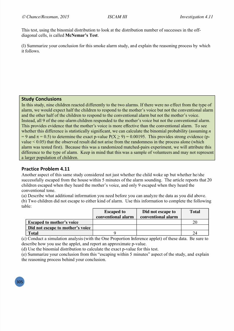
7/25/2019 Text: Investigating Statistical Concepts, Applications, and Methods
http://slidepdf.com/reader/full/text-investigating-statistical-concepts-applications-and-methods 306/428
Chance/Rossman, 2015 ISCAM III Investigation 4.11
#XR
This test, using the binomial distribution to look at the distribution number of successes in the off-diagonal cells, is called McNemar’s Test .
(l) Summarize your conclusion for this smoke alarm study, and explain the reasoning process by whichit follows.
0+456 )'*7$4,8'*, In this study, nine children reacted differently to the two alarms. If there were no effect from the type ofalarm, we would expect half the children to respond to the mother’s voice but not the conventional alarm
and the other half of the children to respond to the conventional alarm but not the mother’s voice.Instead, all 9 of the one-alarm children responded to the mother’s voice but not the conventional alarm.This provides evidence that the mother’s voice is more effective than the conventional alarm. To seewhether this difference is statistically significant, we can calculate the binomial probability (assuming n = 9 and = 0.5) to determine the exact p-value P(X > 9) = 0.00195. This provides strong evidence (p-value < 0.05) that the observed result did not arise from the randomness in the process alone (whichalarm was tested first). Because this was a randomized matched-pairs experiment, we will attribute thisdifference to the type of alarm. Keep in mind that this was a sample of volunteers and may not representa larger population of children.
9:"7+87% 9:'#$%; UDHHAnother aspect of this same study considered not just whether the child woke up but whether he/shesuccessfully escaped from the house within 5 minutes of the alarm sounding. The article reports that 20children escaped when they heard the mother’s voice, and only 9 escaped when they heard theconventional tone.(a) Describe what additional information you need before you can analyze the data as you did above.(b) Two children did not escape to either kind of alarm. Use this information to complete the followingtable:
Escaped toconventional alarm
Did not escape toconventional alarm
Total
Escaped to mother’s voice 20Did not escape to mother’s voice Total 9 24
(c) Conduct a simulation analysis (with the One Proportion Inference applet) of these data. Be sure todescribe how you use the applet, and report an approximate p-value.(d) Use the binomial distribution to calculate the exact p-value for this test.(e) Summarize your conclusion from this “escaping within 5 minutes” aspect of the study, and explainthe reasoning process behind your conclusion.

7/25/2019 Text: Investigating Statistical Concepts, Applications, and Methods
http://slidepdf.com/reader/full/text-investigating-statistical-concepts-applications-and-methods 307/428
Chance/Rossman, 2015 ISCAM III Example 4.1
#XS
Example 4.1: Age Discrimination?Try these questions yourself before you use the solutions following to check your answers.
In Investigation 4.1, you considered the case of Robert Martin and whether the sample of 10 employeesin his department provided evidence of age discrimination. Suppose we decide to focus on the long-run
difference in mean ages for those laid-off and those retained for the decision making process used bythis company.
(a) State the null and alternative hypotheses, in symbols, for this study. [ Hint : Define your symbols.]
(b) Recall the observed value of the sample statistic.
(c) Simulate a randomization test for these data and state your conclusion at the 0.01 level ofsignificance.
(d) Carry out a two-sample t -test for these data and hypotheses, and state your conclusion at the 0.01level of significance.
(e) Do these analyses reach the same conclusion? If not, which analysis should be used? Explain.
<*"$6,8,(a) Let fired not fired represent the difference in the average age of people that would be laid-off, in thelong run (by the overall process), and the average age of the people who would be retained. ( Don’tworry too much at this point about which stage of the firing process this analysis considers. Just keep in
mind that we are trying to say something beyond the observed means. We believe there is someunderlying difference in means and these data provide an estimate.)
H0: fired not fired = 0 (no overall difference in the average ages of those getting fired and not)Ha: fired not fired > 0 (those getting fired will tend to have higher ages than those not)
(b) 21 x x = 58.00 – 41.14 = 16.86 years

7/25/2019 Text: Investigating Statistical Concepts, Applications, and Methods
http://slidepdf.com/reader/full/text-investigating-statistical-concepts-applications-and-methods 308/428
Chance/Rossman, 2015 ISCAM III Example 4.1
#XT
(c) Using the Comparing Groups (Quantitative) applet, the empirical p-value (remembering to match thedirection of subtraction, which may vary depending on how you pasted the data in), the output belowshows an empirical p-value of 0.0225. Because 0.0225 > 0.01, we would not reject the null hypothesis atthe 0.01 level and conclude that this firing process was not more likely to fire individuals with largerages.
Note: You could also carry out this simulation in R. Y ! ,----O A?GG ! -. GC3 &? ?< ,:Y*r
3;3B<AC0 ! 9B084;&BD;*A?GGi?k ! 0;B<&3;3B<AC0i,:(k*)0;B<&3;3B<AC0i]:,-k*
s
(d) A two-sample t -test in Minitab or R:
Now p-value < 0.01, and we would reject the null hypothesis at the 0.01 level and conclude that thisfiring process was more likely to fire individuals with larger ages.
(e) The two-sample t -test yields a much smaller p-value, about 0.006, which implies much strongerevidence of an underlying age difference between the two populations (fired and not fired). However,
because of the small sample sizes (especially with the unbalanced groups), we would have majorconcerns about using the t -procedures for this study. The empirical p-value from the simulatedrandomization test is more trustworthy. In fact, in this stud y, it’s probably more work than we need todo, because with only 120 possible combinations it is not unreasonable to calculate the exact p-value.

7/25/2019 Text: Investigating Statistical Concepts, Applications, and Methods
http://slidepdf.com/reader/full/text-investigating-statistical-concepts-applications-and-methods 309/428
Chance/Rossman, 2015 ISCAM III Example 4.2
#XU
Example 4.2: Speed Limit ChangesTry these questions yourself before you use the solutions following to check your answers.
In 1995, the National Highway System Designation Act abolished the federal mandate of 55 miles perhour maximum speed limit and allowed states to establish their own limits. Of the 50 states (plus
District of Columbia), 32 increased their speed limits in 1996. The data in I5&99')Q&%&-'%',(/%B% shows the percentage change in interstate highway traffic fatalities from 1995 to 1996 and whether or not the stateincreased their speed limit. (Data from the National Highway Traffic Safety Administration as reportedin Ramsey and Schafer, 2002.)
(a) Identify the observational units and response variable of interest. Is this a randomized experiment oran observational study?
(b) Produce numerical and graphical summaries of these data and describe how the two groups compare.
(c) Are the technical conditions for a two-sample t -test met for this study? Explain.
(d) Carry out a two-sample t -test to determine whether the average percentage change in interstatehighway traffic fatalities is significantly higher in states that increased their speed limit. If you find asignificant difference, estimate its magnitude with a confidence interval.
(e) Discuss what the p-value in (d) measures.
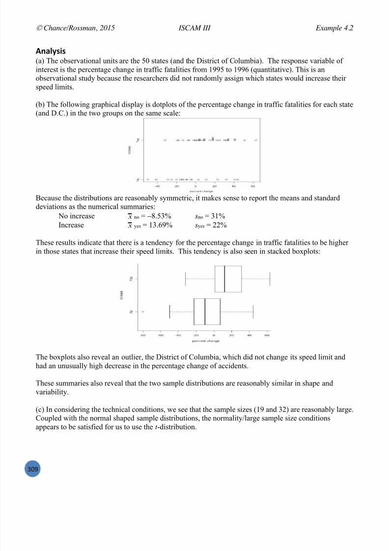
7/25/2019 Text: Investigating Statistical Concepts, Applications, and Methods
http://slidepdf.com/reader/full/text-investigating-statistical-concepts-applications-and-methods 310/428
Chance/Rossman, 2015 ISCAM III Example 4.2
#XV
<*"$6,8,(a) The observational units are the 50 states (and the District of Columbia). The response variable ofinterest is the percentage change in traffic fatalities from 1995 to 1996 (quantitative). This is anobservational study because the researchers did not randomly assign which states would increase theirspeed limits.
(b) The following graphical display is dotplots of the percentage change in traffic fatalities for each state(and D.C.) in the two groups on the same scale:
Because the distributions are reasonably symmetric, it makes sense to report the means and standarddeviations as the numerical summaries:
No increase x no = 8.53% sno = 31%Increase x yes = 13.69% syes = 22%
These results indicate that there is a tendency for the percentage change in traffic fatalities to be higherin those states that increase their speed limits. This tendency is also seen in stacked boxplots:
The boxplots also reveal an outlier, the District of Columbia, which did not change its speed limit andhad an unusually high decrease in the percentage change of accidents.
These summaries also reveal that the two sample distributions are reasonably similar in shape andvariability.
(c) In considering the technical conditions, we see that the sample sizes (19 and 32) are reasonably large.Coupled with the normal shaped sample distributions, the normality/large sample size conditionsappears to be satisfied for us to use the t -distribution.
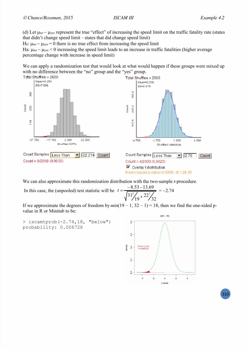
7/25/2019 Text: Investigating Statistical Concepts, Applications, and Methods
http://slidepdf.com/reader/full/text-investigating-statistical-concepts-applications-and-methods 311/428
Chance/Rossman, 2015 ISCAM III Example 4.2
#WX
(d) Let no yes represent the true “effect” of increasing the speed limit on the traffic fatality rate (statesthat didn’t change speed limit – states that did change speed limit)H0: no yes = 0 there is no true effect from increasing the speed limitHa: no yes < 0 increasing the speed limit leads to an increase in traffic fatalities (higher average
percentage change with increase in speed limit)
We can apply a randomization test that would look at what would happen if these groups were mixed upwith n o difference between the “no” group and the “yes” group.
We can also approximate this randomization distribution with the two-sample t -procedure.
In this case, the (unpooled) test statistic will be
3222
1931
69.1353.822
t = 2.74
If we approximate the degrees of freedom by min(19 1, 32 1) = 18, then we find the one-sided p-value in R or Minitab to be:
. ?9IB0783CL&)#=c]Q,aQ 5L;4C>5*83CLBL?4?71: -=--^c#a
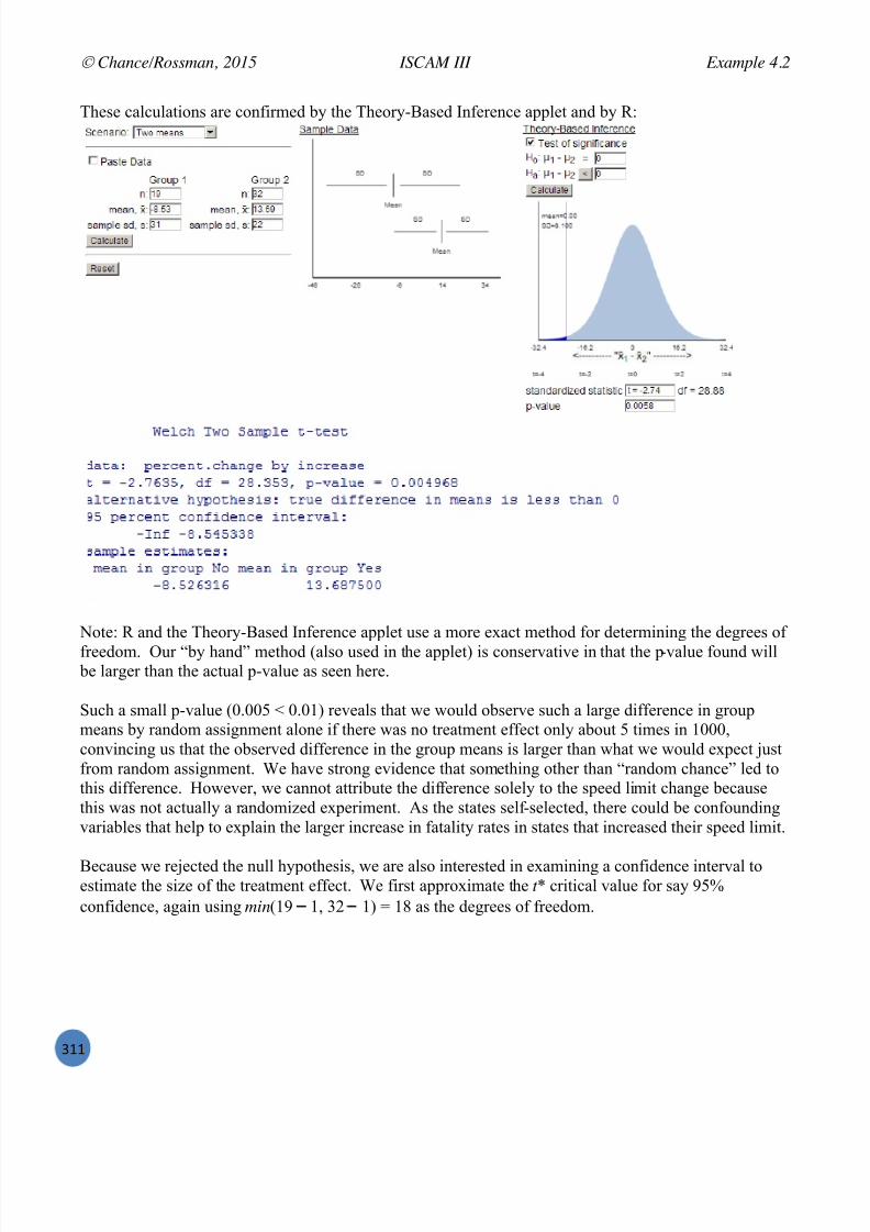
7/25/2019 Text: Investigating Statistical Concepts, Applications, and Methods
http://slidepdf.com/reader/full/text-investigating-statistical-concepts-applications-and-methods 312/428
Chance/Rossman, 2015 ISCAM III Example 4.2
#WW
These calculations are confirmed by the Theory-Based Inference applet and by R:
Note: R and the Theory-Based Inference applet use a more exact method for determining the degrees offreedom. Our “by hand” method (also used in the applet) is conservative in that the p -value found will
be larger than the actual p-value as seen here.
Such a small p-value (0.005 < 0.01) reveals that we would observe such a large difference in groupmeans by random assignment alone if there was no treatment effect only about 5 times in 1000,convincing us that the observed difference in the group means is larger than what we would expect justfrom random assignment. We have strong evidence that something other than “random chance” led tothis difference. However, we cannot attribute the difference solely to the speed limit change becausethis was not actually a randomized experiment. As the states self-selected, there could be confoundingvariables that help to explain the larger increase in fatality rates in states that increased their speed limit.
Because we rejected the null hypothesis, we are also interested in examining a confidence interval toestimate the size of the treatment effect. We first approximate the t * critical value for say 95%confidence, again using min(19 1, 32 1) = 18 as the degrees of freedom.

7/25/2019 Text: Investigating Statistical Concepts, Applications, and Methods
http://slidepdf.com/reader/full/text-investigating-statistical-concepts-applications-and-methods 313/428
Chance/Rossman, 2015 ISCAM III Example 4.2
#W!
. ?9IB0?<H7&=bc_Q ,aQ 5L;4C>5*76; CL9;3HB7?C< >?76 -=bc_ 83CLBL?4?71 L;4C> ?9#=,-,
Then the 95% confidence interval can be calculated,
3221
193110092.269.1353.8
22 = 22.2 16.85
We are 95% confident that the true “treatment effect” is in this interval or that the mean percentageincrease in traffic fatality rates is between 5.4 percentage points to 39.1 percentage points higher instates that increase their speed limit compared to states that do not increase their speed limit (continuingto be careful not to state this as a cause and effect relationship).
Before we complete this analysis, it is worthwhile to investigate the amount of influence that theoutlier (the District of Columbia) has on the results, especially because D.C. does have differentcharacteristics from the states in general. The updated R output (two-sided p-value) is below:
As we might have guessed, the mean increase in fatalities for the “No” group has increased sothat the difference in the group means is less extreme. This leads to a less extreme test statistic and alarger p-value (one-sided p-value = 0.01785/2 = 0.0089) so somewhat weaker evidence against the nullhypothesis in favor of the one-sided alternative hypothesis.
(e) The other technical condition is that we have independent random samples or random assignment togroups. We do not have either in this study, because we are examining the population of all states (andD.C.), and the states self-selected whether they changed their speed limit. Thus, any p-value wecalculate is in a sense hypothetical because we have all the states here, we might ask the question: wouldthe two groups look this different if whether or not they increased their speed limit had been assigned at
random?So the above p-value measures how often we would see a difference in group means at least thislarge based on random assignment to the two groups if there were no true treatment effect. Even thoughthis p-value is hypothetical, we still have some sense that the difference observed between the groups islarger than we would expect to see “by chance” even in a situation like this where it is not feasible tocarry out a true randomized experiment. This gives some information that can be used in policydecisions but we must be careful not to overstate the attribution to the speed limit change.

7/25/2019 Text: Investigating Statistical Concepts, Applications, and Methods
http://slidepdf.com/reader/full/text-investigating-statistical-concepts-applications-and-methods 314/428
Chance/Rossman, 2015 ISCAM III Example 4.3
#W#
Example 4.3: Distracted Driving?Try these questions yourself before you use the solutions following to check your answers.
Recall the Distracted Driving study from Example 2.2. The reaction times (in milliseconds) for 16students appear below and in the file ;5'4'.3/%B%.
Subject A B C D E F G H I J K L M N O PCell 636 623 615 672 601 600 542 554 543 520 609 559 595 565 573 554Control 604 556 540 522 459 544 513 470 556 531 599 537 619 536 554 467
(a) Analyze the differences in reaction times (cell phone minus control) for these subjects. Includenumerical and graphical summaries of the distribution of differences. Comment on what this descriptiveanalysis reveals about whether talking on a cell phone tends to produce slower reaction times.
(b) State the appropriate null and alternative hypotheses to be tested, in order to investigate the researchquestion of whether talking on a cell phone tends to produce slower reaction times.
(c) Conduct a simulation analysis of a randomization test for testing these hypotheses. Report theempirical p-value. Summarize the conclusion that you would draw from this analysis.
(d) Comment on whether the conditions for applying a paired t -test and t -interval are satisfied for thesedata.
(e) Conduct a paired t -test of these hypotheses. Report the value of the test statistic and the p-value.Indicate your test decision at the 0.05 and 0.01 significance levels, and summarize your conclusion.
(f) Produce and interpret a 95% t -confidence interval for the population mean difference. Also produceand interpret a 95% prediction interval. Comment on how these two intervals compare.
(g) Compare these analyses to that in Example 2.2. Which analysis would you recommend and why?

7/25/2019 Text: Investigating Statistical Concepts, Applications, and Methods
http://slidepdf.com/reader/full/text-investigating-statistical-concepts-applications-and-methods 315/428
Chance/Rossman, 2015 ISCAM III Example 4.3
#WP
<*"$6,8,(a) Analyzing the differences
The sample mean difference in reaction times (cell minus control) is d x = 47.125 milliseconds, with astandard deviation of sd = 51.331 milliseconds. The dotplot reveals that most of the differences are
positive, suggesting that subjects talking on a cell phone tend to take longer to react than subjectslistening to a book-on-tape.
(b) The null hypothesis says that the mean reaction time is the same among cell phone users as among book-on-tape listeners (H 0: cell – control = 0). The alternative says that the mean reaction time is largeramong cell phone users than among book-on-tape listeners (H a: cell – control > 0).
(c) We can carry out the simulation easily with the applet or with R.
Copying and pasting the data into the Matched Pairs appletwith 1,000 repetitions we get the results shown here.
Using R to carry out the simulation instead:N;B<%?GG9!-GC3 &? ?< ,:,----*r
0247?84?;3!9B084;&I&),Q,*Q ,^Qm 3;84BI;!UPJ'*
PB<AC0?d;A%B7B!A?GG;3;<I;9+0247?84?;3N;B<%?GG9i?k!0;B<&PB<AC0?d;A%B7B*s
L:'; @I The empirical p-value is the proportion of these 10,000 repetitions in which the mean differenceis 47.125 or more, because 47.125 is the value of the sample mean difference from the actualexperimental data. None of the 10,000 repetitions produced such a large mean difference, so theempirical p-value is 0. The simulation therefore shows that we would almost never get a result asextreme as the actual experiment did, if there were really no difference between reactions to cell phone

7/25/2019 Text: Investigating Statistical Concepts, Applications, and Methods
http://slidepdf.com/reader/full/text-investigating-statistical-concepts-applications-and-methods 316/428
Chance/Rossman, 2015 ISCAM III Example 4.3
#WR
vs. book-on-tape, so we have extremely strong evidence that the cell phone really does increase reactiontimes.
(d) Because the sample size (16) is fairly small, the t -procedures are valid only if the population ofdifferences follows a normal distribution. The dotplot of differences from these 16 subjects looks
roughly symmetric, so the t -procedures are probably valid to apply here.
(e) The test statistic isd d
d
ns
x 0 =
16331.51
125.47 ≈ 3.67 . The p-value is the probability that a t -
distribution with 15 degrees of freedom is 3.67 or larger; R reveals this p-value to be 0.001137. This p-value is very small, so we would reject the null hypothesis at the 0.05 and 0.01 significance levels. Theexperimental data provide very strong evidence that talking on a cell phone does cause an increase inmean reaction time, as compared to listening to a book-on-tape. The cause/effect conclusion is justified
because this is a randomized experiment with a very small p-value.
Note: This evidence is stronger than what we saw with the sign test in Example 2.2.
(f) A 95% confidence interval for the population mean difference d is: d x ± t *!d d ns , which is
47.125 ± 2.131(51.331)/ 16 , which is 47.125 ± 27.347, which is (19.778, 74.472). We can be 95%confident that the mean reaction time while talking on a cell phone is between roughly 20 and 75milliseconds longer than when listening to a book-on-tape.A 95% prediction interval for the difference in reaction times for a particular subject is:
d x ± t * d d ns /11 , which is 47.125 ± 2.131(51.331) 16/11 , which is 47.125 ± 112.753, which is
( 64.628, 159.878). We can be 95% confident that the an individual subject will react anywhere from65 milliseconds more quickly to 160 milliseconds more slowly talking on a cell phone as compared tolistening to a book-on-tape.
(g) An advantage of the sign test from Chapter 2 is we don’t need to rely on large sample sizes ornormality of the differences for the procedure to be valid. However, by ignoring some information in thedata, we would expect this procedure to have lower power and we lose information about the size of thedifference. The conditions for the t- procedure seem to be satisfactorily met here.

7/25/2019 Text: Investigating Statistical Concepts, Applications, and Methods
http://slidepdf.com/reader/full/text-investigating-statistical-concepts-applications-and-methods 317/428
Chance/Rossman, 2015 ISCAM III Chapter 4 Summary
#WS
).<9!/@ U 01BB<@_
In this chapter, you have again focused on comparing the outcomes for different groups, but forquantitative data. The tools for descriptive statistics are the same as in chapter 2 (e.g., means, medians,standard deviations, interquartile ranges, dotplots, histograms, and boxplots).
After exploring and comparing the groups descriptively, it may be appropriate to ask whether thedifferences observed could have arisen “by chance alone .” In other words, is the observed differencelarge enough to convince us that it arose from a genuine difference in the groups instead of from therandomness inherent in designing the experiment or in selecting the samples? Analogous to comparing
proportions in Chapter 3, we used simulation to approximate how often we would obtain a difference inmeans at least as extreme as observed just by chance (random sampling or random assignment). Thenwe learned of a “large sample” approach we can use in either case to approximate the null distribution ofthe standardized statistic, yielding the two-sample t -test. Keep in mind that the logic of statisticalsignificance hasn’t changed – we assume there is no effect or no population difference and determinehow often we would get a sample difference result at least as extreme as what was observed. You saw
that this chance is strongly affected by the amount of variability within the groups. It is very importantwhen reporting on your statistical study that you also mention the sample sizes. This helps you evaluatethe power and practical significance of the study results. You were also reminded that no matter howsmall a p-value is, we cannot draw cause-and-effect conclusions unless the data came from a properlydesigned randomized experiment.
You will often have the choice between a randomization-based test or the t -produces. The advantage tothe randomization procedures is they allow us to work with many types of statistics (such as median andtrimmed mean) where we do not have theoretical results on the large sample behavior of therandomization distribution. The advantage of the t -procedures is the ease in calculating confidenceintervals. It is always important to consider the technical conditions of an inference procedure before
applying the procedure (e.g., make sure you really have two independent samples). If data are paired,then you should consider one-sample procedures on the differences. Such pairing is often very useful inincreasing the efficiency of the study. These t -procedures are quite robust in calculating p-values andconfidence intervals.
Always keep in mind the importance of considering whether there is random sampling and/or randomassignment in the study design and how that impacts the scope of conclusions that you can draw fromyour study.
01BB<@_ -L `.<! _-1 .<J/ K/<@3/2 M3 !.M0 ).<9!/@ Stating hypotheses in terms of comparing two population or underlying treatment means The reasoning process behind a randomization test
C Calculating and interpreting p-values Two-sample t- procedures for comparing two groups
C When appropriate to apply, why helpfulC How to interpret resultsC Alternative approaches if not valid (e.g., data transformations)
Using technology to calculate two-sample t -procedures

7/25/2019 Text: Investigating Statistical Concepts, Applications, and Methods
http://slidepdf.com/reader/full/text-investigating-statistical-concepts-applications-and-methods 318/428
Chance/Rossman, 2015 ISCAM III Chapter 4 Summary`
#WT
Factors that affect the significance of the comparison (e.g., sample size, size of difference, andwithin-group variability)
Methods for reducing within-group variability Matched-pairs designs and analyses
!/).3-K-N_ 01BB<@_ Simulating a randomization test for different statistics Two-sample t -procedures Paired t -procedures
a487Q @%(%:%*7% +' M0)<B `':Q,?"7% L4*7+8'*, "*5 '+=%: @ )';;"*5,
9:'7%54:% 2%,8:%5 L4*7+8'* 3";% O'?+8'*,P$%&)>,; E1%8-1% '()&*;1%8-1% F5,(81.(,7 ,B8-&.&%1567 .&*,(G$%&)> ;&%& (%&)>F;&%&o7 )F`4&5W`7 `4&5!`GpGO&5&--,- E1%8-1%( F(%&)>,; ;&%&G '()&*;1%8-1% F5,(81.(,7 ,B8-&.&%156GO&5&--,- j'(%135&*( F(%&)>,; ;&%&G \1&; \&%%'), 8&)>&3,7 %+,. +'(%135&* Fq5,(81.(, r
,B8-&.&%1567 -&612%_)FW7!GGO&5&--,- M1B8-1%( F(%&)>,; ;&%&G =1B8-1%F5,(81.(,q,B8-&.&%1567 +15'K1.%&-_I[ZfG]2*,5')&- $2**&5',( '()&*(2**&56F5,(81.(,7 ,B8-&.&%156G%<1:(&*8-, , :851),;25,( %/%,(%F5,(81.(,q,B8-&.&%1567 &-%7 4&5/,A2&-_Q0\$fG%<1:(&*8-, , : 851),;25,( F(2**&56 ;&%&G '()&*%<1(&*8-,%FBW7 (W7 .W7 B!7 (!7 .!7 +681%+,('K,;7
&-%,5.&%'4,7 )1.9/-,4,-GO&'5,; , :%,(% %/%,(%F4W7 4!7 &-%,5.&%'4,7 )1.9/-,4,-7 8&'5,;_I[ZfG
a487Q @%(%:%*7% +' B8*8+"# )';;"*5,
9:'7%54:% 2%,8:%5 B%*4$%&)>,; ;1%8-1%( F(%&)>,; ;&%&G b5&8+ a E1%8-1%7 L., D7 J'%+ b5128($%&)>,; ;1%8-1%( F2.(%&)>,;G b5&8+ a E1%8-1%, Multiple Y’s, Simple $%&)> ;&%& E&%& a $%&)> a N1-2*.(
L5 CIMa (%&)> )W )! )#s $ZMNa (2=( )P/O&5&--,- j'(%135&*( F2.(%&)>,;G b5&8+ a j'(%135&*7 $'*8-,7 C2-%'8-, b5&8+(]2*,5')&- $2**&5',( $%&% a M&(') $%&%'(%')( a E'(8-&6 E,()5'8%'4, $%&%'(%')( <'%+ M6
k&5'&=-,%<1:(&*8-, , :851),;25,( F(%&)>,; ;&%&G $%&% a M&(') $%&%'(%')( a !:$&*8-, %7 $&*8-,( '. 1., )1-2*.%<1:(&*8-, , :851),;25,( F2.(%&)>,; ;&%&G $%&% a M&(') $%&%'(%')( a !:$&*8-, %7 $&*8-,( '. ;'99,5,.%
)1-2*.(%<1:(&*8-, , :851),;25,( F(2**&56 ;&%&G $%&% a M&(') $%&%'(%')( a !:$&*8-, %7 $2**&5'K,; ;&%&O&'5,; , %,(% $%&% a M&(') $%&%'(%')( a O&'5,; %

7/25/2019 Text: Investigating Statistical Concepts, Applications, and Methods
http://slidepdf.com/reader/full/text-investigating-statistical-concepts-applications-and-methods 319/428
Chance/Rossman, 2015 ISCAM III Chapter 4 Summary
#WU
)='87% '( 9:'7%54:%, (': )';?":8*> !G' B%"*,
Parameter Difference in populationmeans or treatment means( )
Difference in populationmedians or treatmentmedians
Mean difference
Study design Randomized experiment orindependent random samples
Randomized experiment orindependent random samples
Matched paireddesign
Null Hypothesis H0: 21 = 0 H0: population mediansequal
H0: diff = 0
Simulation Randomly assign response values between groups (seeComparing Groups (Quantitative) applet)
Flip a coin to seewhether to flip theorder of theobservations
Exact p-value All possible random assignmentsValid to use t-procedures if
Both sample sizes at least 30or both populationdistributions normal N/A
At least 30differences ordifferences arenormal
Test Statistic t 0= − 2 2+222 N/A = 0/√
Confidenceinterval ( x 1 x 2) t *
2
22
1
21
n
s
n
s
x t *n 1 s/ n
Predictioninterval
x t *n 1 sn/11
R Commands '()&*%<1(&*8-,% mean1, stddev1, n1,mean2, stdev2, n2
Optional: hypothesizeddifference and alternative (“less”, “greater”, or“two.sided”)
Optional: conf.level
%/%,(%F5,(8q,B87 &-%74&5/,A2&-_Q0\$fG
%/%,(% F-'(%W7 -'(%!7&-%7 )1.9/-,4,-78&'5,;_I[ZfG
Minitab $%&% a M&(') $%&%'(%')( a !:(&*8-, %
$%&% a M&(')$%&%'(%')( a O&'5,; %
TBI applet I<1 *,&.(
Note: You can also consider transforming the data before applying normal-based methods

7/25/2019 Text: Investigating Statistical Concepts, Applications, and Methods
http://slidepdf.com/reader/full/text-investigating-statistical-concepts-applications-and-methods 320/428
Chance/Rossman, 2015 ISCAM III Chapter 5
#WV
CHAPTER 5: COMPARING SEVERAL POPULATIONS, EXPLORING RELATIONSHIPS
The idea of comparing two groups has been a recurring theme throughout this course. In the previouschapters, you have been limited to exploring two groups at a time. You saw that often the same analysistechniques apply whether the data have been collected as independent random samples or from a randomizedexperiment, although this data collection distinction strongly influences the scope of conclusions that youcan draw from the study. You will see a similar pattern in this chapter as you extend your analyses toexploring two or more groups. In particular, you will study a procedure for comparing a categorical responsevariable across several groups and a procedure for comparing a quantitative response variable across severalgroups. You will also study the important notion of association between variables, first with categoricalvariables and then for studies in which both variables are quantitative. In this latter case, you will also learn anew set of numerical and graphical summaries for describing these relationships.
Section 1: Two Categorical VariablesInvestigation 5.1: Dr. Spock’s t rial – Chi-square test for homogeneity of proportionsInvestigation 5.2: Nightlights and near-sightedness (cont.) – Chi-square test for associationTechnology Exploration: Randomization test for chi-square statisticInvestigation 5.3: Newspaper credibility decline – Comparing distributions
Section 2: Comparing Several Population MeansInvestigation 5.4: Disability discrimination – Reasoning of ANOVAApplet Exploration: Randomization test for ANOVAInvestigation 5.5: Restaurant spending and music – ANOVA practiceApplet Exploration: Exploring ANOVA
Section 3: Two Quantitative VariablesInvestigation 5.6: Cat jumping – ScatterplotsInvestigation 5.7: Drive for show, putt for dough – Correlation coefficientsApplet Exploration: Correlation guessing gameInvestigation 5.8: Height and foot size – Least squares regressionApplet Exploration: Behavior of regression lines – ResistanceExcel Exploration: Minimization criteriaInvestigation 5.9: Money-making movies – Application
Section 4: Inference for RegressionInvestigation 5.10: Running out of time – Inference for regression (sampling)Investigation 5.11: Running out of time (cont.) – Inference for regression (shuffling)Investigation 5.12: B oys’ heights – Regression modelInvestigation 5.13: Cat jumping (cont.) – Confidence intervals for regression
Investigation 5.14: Housing prices – TransformationsTechnology Exploration: The regression effect
Example 5.1: Internet Use by RegionExample 5.2: Lifetimes of NotablesExample 5.3: Physical Education Class PerformanceExample 5.4: Comparing Popular Diets
! " # $ % & ' ( ) & ' " (
+ & ) & ' % & ' , )
- . / " , $ 0 & % 1
2 0 0
- ' , ) & ' / " % 1 ) "
3 4 $ & 5 /
3 %
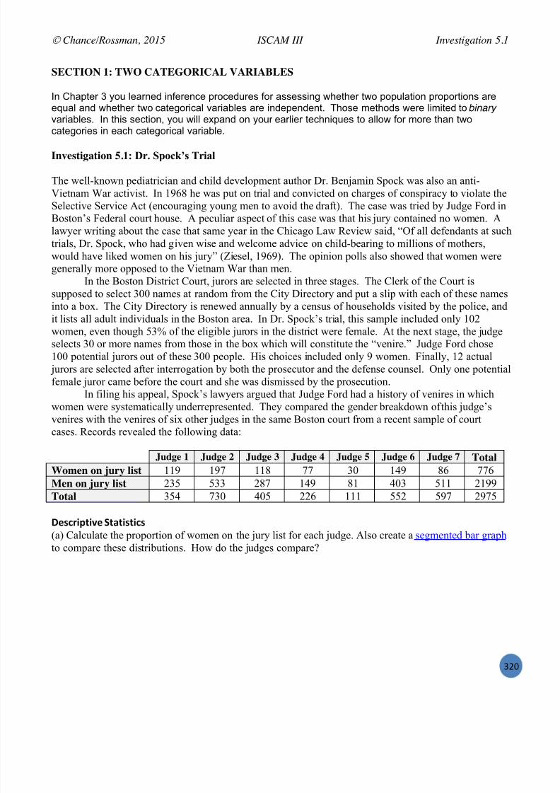
7/25/2019 Text: Investigating Statistical Concepts, Applications, and Methods
http://slidepdf.com/reader/full/text-investigating-statistical-concepts-applications-and-methods 321/428
Chance/Rossman, 2015 ISCAM III Investigation 5.1
#!X
SECTION 1: TWO CATEGORICAL VARIABLES
In Chapter 3 you learned inference procedures for assessing whether two population proportions areequal and whether two categorical variables are independent. Those methods were limited to binary variables. In this section, you will expand on your earlier techniques to allow for more than twocategories in each categorical variable.
Investigation 5. 1: Dr. Spock’s Trial
The well-known pediatrician and child development author Dr. Benjamin Spock was also an anti-Vietnam War activist. In 1968 he was put on trial and convicted on charges of conspiracy to violate theSelective Service Act (encouraging young men to avoid the draft). The case was tried by Judge Ford inBoston’s Federal court house. A peculiar aspect of this case was that his jury contained no women. Alawyer writing about the case that same year in the Chicago Law Review said, “Of all defendants at suchtrials, Dr. Spock, who had given wise and welcome advice on child-bearing to millions of mothers,would have liked women on his jury” (Ziesel, 1969). The opinion polls also showed that women weregenerally more opposed to the Vietnam War than men.
In the Boston District Court, jurors are selected in three stages. The Clerk of the Court issupposed to select 300 names at random from the City Directory and put a slip with each of these namesinto a box. The City Directory is renewed annually by a census of households visited by the police, andit lists all adult individuals in the Boston area. In Dr. Spock’s trial, this sample included only 102women, even though 53% of the eligible jurors in the district were female. At the next stage, the judgeselects 30 or more names from those in the box which wi ll constitute the “venire.” Judge Ford chose100 potential jurors out of these 300 people. His choices included only 9 women. Finally, 12 actual
jurors are selected after interrogation by both the prosecutor and the defense counsel. Only one potentialfemale juror came before the court and she was dismissed by the prosecution.
In filing his appeal, Spock’s lawyers argued that Judge Ford had a history of venires in whichwomen were systematically underrepresented. They compared the gender breakdown of this judge’svenires with the venires of six other judges in the same Boston court from a recent sample of courtcases. Records revealed the following data:
Judge 1 Judge 2 Judge 3 Judge 4 Judge 5 Judge 6 Judge 7 TotalWomen on jury list 119 197 118 77 30 149 86 776Men on jury list 235 533 287 149 81 403 511 2199Total 354 730 405 226 111 552 597 2975
2%,7:8?+8F% 0+"+8,+87, (a) Calculate the proportion of women on the jury list for each judge. Also create a segmented bar graph to compare these distributions. How do the judges compare?

7/25/2019 Text: Investigating Statistical Concepts, Applications, and Methods
http://slidepdf.com/reader/full/text-investigating-statistical-concepts-applications-and-methods 322/428
Chance/Rossman, 2015 ISCAM III Investigation 5.1
#!W
(b) Let i represent the probability of judge i selecting a female for the jury list. State a null and analternative hypothesis for testing whether these data provide reason to doubt that the proportion ofwomen on jury lists is the same for all seven judges.
Note : Your null hypothesis states only that the probabilities are equal; you are not specifying a particularvalue for this common probability. The alternative hypothesis can state only that at least one probabilitydiffers from the rest.
If the null hypothesis is true, then the long-run probability of a woman on the jury panel equalsthe same value for all seven judges.
34$$ B'5%$
(c) Suggest an estimate for this common (across all judges) probability that a juror is female.
(d) How many jurors were on Judge 1 ’s list ? If you suppose the long-run proportion of women in his juries was 0.261, how many of these jurors would you expect to be female? How many would youexpect to be male? ( Recall : An “expected value” does not need to be an integer.)
Female:
Male:(e) How many of the jurors on Judge 2 ’s list would you expect to be female if his long-run proportionwas also 0.261? How many would you expect to be male?
Female:
Male:
(f) Enter your expected counts below the observed counts in the following table.Judge
1
Judge
2
Judge
3
Judge
4
Judge
5
Judge
6
Judge
7Women on jury list
Observed
Expected
119 197 118
105.71
77
58.99
30
28.97
149
144.07
86
155.82
Men on jury listObserved
Expected
235 533 287
299.30
149
167.01
81
82.03
403
407.93
511
441.18 Total 354 730 405 226 111 552 597

7/25/2019 Text: Investigating Statistical Concepts, Applications, and Methods
http://slidepdf.com/reader/full/text-investigating-statistical-concepts-applications-and-methods 323/428
Chance/Rossman, 2015 ISCAM III Investigation 5.1
#!!
(g) Are the observed counts equal to the expected counts in each cell of the table? Is it possible that thelong-run probability of a female jury panel member is the same for each judge, and the differences
between the observed counts and the expected counts found in the table are due to random chancealone?
!%,+ 0+"+8,+87(h) Suggest a statistic for measuring the overall deviation between the observed counts and the expectedcounts. [ Hint : Write your statistic as a formula or rule for obtaining one number that takes into accountinformation in the sample relevant to comparing all seven groups.]
A common test statistic used to compare the observed and expected counts in a two-way table is theChi-squared test statistic :
r
i
c
j ij
ij ij
ected exp
ected expobserved
1 1
22
where r = number of rows and c = number of columns. This test statistic looks at the discrepancy between the observed and expected counts for each cell, squares the difference to ensure a positivecontribution , “standardiz es” by dividing by the expected count, and then sums across all cells.
(i) Calculate this test statistic for the above two-way table. [ Hint : Fill in the terms for the first two judges and then sum all of values together.]
18.441)18.441511(
93.407)93.407403(
03.82)03.8281(
01.167)01.167149(
30.299)30.299287(
82.155)82.15586(
07.144)07.144149(
97.28)97.2830(
99.58)99.5877(
71.105)71.105118(
22222
222222
(j) What types of test statistic values (large, small, positive, negative) constitute evidence against the nullhypothesis of equal long-run probabilities? Explain.
02.1106.001.095.151.0
22.3117.004.053.545.12

7/25/2019 Text: Investigating Statistical Concepts, Applications, and Methods
http://slidepdf.com/reader/full/text-investigating-statistical-concepts-applications-and-methods 324/428
Chance/Rossman, 2015 ISCAM III Investigation 5.1
#!#
08;4$"+8'*In order to approximate the p-value of this test, we need to examine how the test statistic varies underthe null hypothesis of equal probabilities. We will once again explore this null distribution first bysimulating a large number of random samples where the probability of a juror being female is the samefor each judge (under the null hypothesis).
(k) Outline the steps you would use to generate random data for each judge under the null hypothesisthat the probability of a juror being female is the same for each judge.
(l) Use a premade script or macro to carry out the simulation:
M* @I Run the $81)>/[ script to generate 1000 chi-square values. M* B8*8+"#: Use the $81)>$'*/*&) macro to generate 500 chi-square values. (Save an emptyworksheet and the macro in the same folder so you can use type NUe. XK8CI@K?0=0BI .)
(m) Describe the shape, center, and variability of the simulated null distribution.
(n) Based on your simulation, determine the proportion of simulated test statistic values that are as large
or larger than the test statistic value you computed in (i). Does this empirical p-value provideconvincing evidence that the difference between observed and expected counts that you observed islarger than we would expect by chance? What do you conclude about whether the seven judges all hadthe same long-run probability of a juror being female? Explain.
B"+=%;"+87"$ B'5%$Rather than rely on simulation to produce (approximate) p-values for this test, we can use a probabilitymodel to approximate the sampling distribution of the chi-square test statistic. We just need to find theright one.
(o) Use technology to determine whether a normal probability distribution appears to adequately predict the behavior of the simulated null distribution of this test statistic:

7/25/2019 Text: Investigating Statistical Concepts, Applications, and Methods
http://slidepdf.com/reader/full/text-investigating-statistical-concepts-applications-and-methods 325/428
Chance/Rossman, 2015 ISCAM III Investigation 5.1
#!P
M* @I To create a normal probability plot: > \\<C30&I6?9\HB42;9* M* B8*8+"#IChoose Graph > Probability Plot , then press OK (for Single), double click on
the column with the simulated chi-square values so it appears in the Graph variables box.Press OK .
What is your assessment?
(p) Use technology to whether a “chi -square” probability model appears to adequately predict the behavior of the simulated null distribution of this test statistic:Create a probability plot for the chi-square distribution with 6 degrees of freedom.
M* @I Create a qqplot with data randomly generated from a chi-square distribution> \\84C7&I6?9\920Q \I6?9\&88C?<79&,---*QAG ! ^**
M* B8*8+"#IThis is equivalent to a Gamma distribution with parameters shape = 6/2 = 3 and scale= 2. Double click on the blue guidelines in the probability plot. Then in the Edit distribution Fitwindow, select the Gamma distribution under the Options tab.
(q) What is your assessment of the fit of this model to the simulated test statistic values?
The Chi-Square distribution is skewed to the right and provides a reasonable model to the above teststatistic for large sample sizes. We will consider the chi-square distribution model appropriate if all ofthe expected counts are at least 1 and if at least 80% of the expected counts are at least 5.
When comparing several population proportions, the chi-square degrees of freedom are equal to thenumber of explanatory variable categories minus 1, c 1. This makes sense because once we specifythe number of observations in c 1 of the categories, the last category is forced to assume the value thatallows the observed counts to sum to the sample size.
For large sample sizes, we will use the chi-square distribution to approximate the p-value.
!%7=*'$'>6 2%+'4: – )=8\,c4":% 9:'#"#8$8+8%,
M* @IThe '()&*)+'(A851= function takes the following inputs xval = the observed value of the test statistic df = degrees of freedom for the chi-square distribution
M* B8*8+"#IChoose Graph > Probability Distribution Plot (View Probability) . Then select theChi-Square distribution with Degrees of freedom = 6. Select the Shaded Area tab, and specify theX value , with Right Tail , to be 62.68. Press OK .
(r) How does this p-value compare to the empirical p-value you determined in (n)?

7/25/2019 Text: Investigating Statistical Concepts, Applications, and Methods
http://slidepdf.com/reader/full/text-investigating-statistical-concepts-applications-and-methods 326/428
Chance/Rossman, 2015 ISCAM III Investigation 5.1
#!R
Discussion: If the null hypothesis is rejected, the conclusion we draw is that at least one of the population proportions differs from the rest, but we don’t have much information ab out which one. Itcould be that one explanatory variable group is behaving much differently than the rest or they could all
be different. One way to gain more information about the nature of the differences between the i values is to compare the components of the chi-square statistic sum.
(s) Return to the sum you calculated in (i). Which cell comparison(s) provide the largest (standardized)discrepancy between the observed counts and the expected counts?
(t) For the cells identified in (s), which is larger, the observed counts or the expected counts? Explainthe implications of this comparison.
(u) Which judge do you believe tried Dr. Spock’s case? Explain.
0+456 )'*7$4,8'*,
One judge clearly stood out compared to the others in these sample data. If we consider theseresults to be representative of the overall jury selection process, the very small p-value indicatesthat if in fact the judges’ selections of jurors were independent random processes with the same
probability of selecting a woman, then it would be almost impossible to observe sample proportions differing by this much by chance alone. Thus, the sample data provide strongevidence that the long-run probability of a juror being female is not the same among all seven
judges. The largest contributions to the X 2 test statistic, by far, come from judge 7, who hasmany more men than would be expected and many fewer women than would be expected on his
jury lists. This was indeed Judge Ford, the judge assigned to Dr. Spock’s case. In fact, there aretwo issues with this judge: The sampling from the city directory led to a far smaller percentage ofwomen (29%) than the city population (53%) across all the judges, and then the proportion of
women selected by Judge Ford dipped even lower to around 15% women. (By the way, the Courtof Appeals reversed Spock’s conviction on other grounds without reaching the jury selectionissue.) Although this p-value is hypothetical in nature (there was not a true random mechanismused in generating these outcomes), and we cannot draw a cause-and-effect conclusion because ofthe observational nature of the data, the p-value does provides a measure of how very surprisingthese results would be to occur by chance alone.

7/25/2019 Text: Investigating Statistical Concepts, Applications, and Methods
http://slidepdf.com/reader/full/text-investigating-statistical-concepts-applications-and-methods 327/428
Chance/Rossman, 2015 ISCAM III Investigation 5.1
#!S
!%7=*87"$ )'*58+8'*,The chi-square distribution is an approximation to the sampling distribution of the chi-square teststatistic when the data arise from independent binomial random variables. This approximation isconsidered valid as long as the average expected cell count is at least 5 and all of the individual expectedcell counts are at least one. Notice we are discussing the expected cell counts here, not the observed cell
counts. The data also need to have been collected from independent random samples or from arandomized comparative experiment.
The advantage of a Chi-Square Test is that it provides an overall p-value for all the comparisons at oncewhich controls the overall probability of a Type I error. If the p-value is not significant, we usually donot check all of the individual comparisons. If the p-value is significant, then we can do more formalfollow-up analyses to see where the difference(s) are arising. If we run many tests on the same data set,we are always concerned about an inflated overall Type I error rate.
04;;":6 '( )=8\0c4":% !%,+ '( .';'>%*%8+6 '( 9:'?':+8'*,
Numerical and graphical summaries: conditional proportions and segmented bar graphs
If the data are independent random samples from I different populations or processes and at least80% of the expected cell counts are at least 5 (and all are at least one), then the hypotheses
H0: 1 = … = I where i is the probability of success in population i.Ha: at least one i differs from the rest
can be tested using the chi-square teststatistic:
2
1 1
22
i
I
j ij
ij ij
ected exp
expected observed
The (upper-tail) p-value is calculated from the chi-square distribution with ( I 1) degrees offreedom.
Note: The chi-square calculations are not affected by which variable you treat as explanatory and whichas response.
9:"7+87% 9:'#$%; VDH
One question that you may be asking is why not just use the two-sample z procedures to compare pairsof proportions? We could do this for two groups at a time, e.g., comparing Judge 1 to Judge 2 and thenJudge 3 to Judge 5 and so on.(a) How many such two-group comparisons are there among these 7 judges?(b) If the level of significance is set to 0.05, what is the probability of a Type I error for any one of thesecomparisons?(c) What about the probability of at least one Type I error among these 21 comparisons – will that belarger or smaller than 0.05? Explain.

7/25/2019 Text: Investigating Statistical Concepts, Applications, and Methods
http://slidepdf.com/reader/full/text-investigating-statistical-concepts-applications-and-methods 328/428
Chance/Rossman, 2015 ISCAM III Investigation 5.1
#!T
!%7=*'$'>6 2%+'4: – )=8\0c4":% !%,+,
M* @ If you have the counts for the two-way table, can pass the table using the matrix command:. 98CI@7BL4; ! 0B73?[&I&,,bQ #(_Q ,bcQ _((Q ,,aQ #acQ ccQ ,]bQ
(-Q a,Q ,]bQ ]-(Q a^Q _,,*Q <IC4!c*. I6?9\=7;97&98CI@7BL4;* For the raw data (e.g., in 98CI@ ), create and pass in the frequency table, e.g.,
. I6?9\=7;97&7BL4;&98CI@**
M* B8*8+"# If the two way table has been entered into
I columns, choose Stat > Tables > Chi-Square Test for association . Use the pulldown menu to select Summarizeddata… and the specify the columnscontaining the observed counts.
Click OK .
If the raw data for each categoricalvariable are contained in two differentcolumns, choose Stat > Tables > CrossTabulation and Chi-Square . Leave“Raw data” selected in the drop -downmenu.
Specify the two variables rows andcolumns . Press the Chi-Square buttonand select “Chi -Square Analysis” to bedisplayed. Click OK twice.
When checking the Chi-square test box, you can also ask Minitab to report the expectedcounts, and the cell contributions (the terms being summed together to determine the chi-square statistic).
M* <*"$6E8*> !G'\G"6 !"#$%, "??$%+ Paste either the raw data (press Use
Data ) or the two-way table (press UseTable ) into the Sample data box, using
one word category names. Check the Show X 2 Output box.
The applet reports the observed 2 value, df,and cell contributions. (You can expand thiswindow by dragging out the lower rightcorner. Check the Show table box to see theobserved counts.)

7/25/2019 Text: Investigating Statistical Concepts, Applications, and Methods
http://slidepdf.com/reader/full/text-investigating-statistical-concepts-applications-and-methods 329/428
Chance/Rossman, 2015 ISCAM III Investigation 5.2
#!U
Investigation 5.2: Nightlights and Near-sightedness (cont.)
Recall from Investigation 3.2 we examined a simplified version of the study published by Quinn, Shin,Maguire and Stone (1999) that examined the relationship between the type of lighting children wereexposed to and subsequent eye refraction. Now we are able to look at 3 categories for each variable.
Below is the two way table and segmented bar graph from the study: Dark Night
lightRoomlight
Total
Far-sighted 40 39 12 91Normal 114 115 22 251Near-sighted 18 78 41 137Total 172 232 75 479
(a) What proportion of subjects in this study were classified as being far-sighted? As having normal
vision? As being near-sighted? [ Hint : Looking at the subjects all together now.]
Far-sighted: Normal: Near-sighted:
(b) If the children’s current eye conditions were not related to the level of lighting they were exposed to,what proportion of children in the darkness condition would be far-sighted? Have normal vision? Benear-sighted?
(c) What would the proportional breakdown of eye conditions look like in the night-light group and inthe room-light group if there was no association between eye condition and lighting level?
(d) Use your answers in (b) and (c) to calculate the expected number of children in each cell of the table,assuming that there is no relationship between lighting and eye refraction. [ Hint : For example, multiplythe number of children in the darkness group by the proportion who would have hyperopia in that groupif there were no relationship.] Record your answers in the table below next to the observed counts (thediagonal entries have been done for you).
Expected counts:Darkness Night light Room light Total
Far-sighted 40 ( 32.68 ) 39 ( ) 12 ( ) 91Normal 114 ( ) 115 ( 121.57 ) 22 ( ) 251Near-sighted 18 ( ) 78 ( ) 41 ( 21.45 ) 137Total 172 232 75 479
40 39 12
114
11522
18
7841
0%10%20%30%40%50%60%70%80%90%
100%
Darkness Night l ight Room l ight

7/25/2019 Text: Investigating Statistical Concepts, Applications, and Methods
http://slidepdf.com/reader/full/text-investigating-statistical-concepts-applications-and-methods 330/428
Chance/Rossman, 2015 ISCAM III Investigation 5.2
#!V
If we assume there is no relationship between the explanatory variable and the response variable, we cancalculate the expected count for each cell by calculating
Expected count = Row total Column totalTable total
This produces the same distribution of conditional proportions in each explanatory variable group.
This formula generalizes the approach you used in Investigation 5.1 to tables with more than 2 rowsand more than 2 columns.
(e) Are the observed counts equal to the expected counts in each cell of the above table? Is it possible, ifthere were no relationship between lighting condition and eyesight, that we might have observeddifferences this large just by random chance?
(f) Use technology to calculate a chi-square test statistic to measure the discrepancy between theobserved and expected counts for this table
r
i
c
j ij
ij ij
cted peex
cted peexobserved
1 1
22
where r = number of rows and c = number of columns. (See the previous technology detour to carry outthese calculations in R or Minitab.) What are the values of the chi-square statistic, degrees of freedom,and p-value? [You can also verify the expected counts that you computed in part (d). In R :)+'(A/%,(%F;&%&Ge,B8,)%,;]
Chi-square statistic:
df:
p-value:
The degrees of freedom for the chi-square test statistic with r rows and c columns isdf = ( r 1)(c 1)
(g) Minitab and R also report the chi-square contributions for each cell ( In R : )+'(A/%,(%F;&%&Ge5,(';2&-( for the unsquared versions). Which cell(s) contribute the most to the overall chi-square sum? Comparethe observed counts to the expected counts for those cells. What do these comparisons reveal about thenature of the relationship between children’s eye condition and level of lighting?
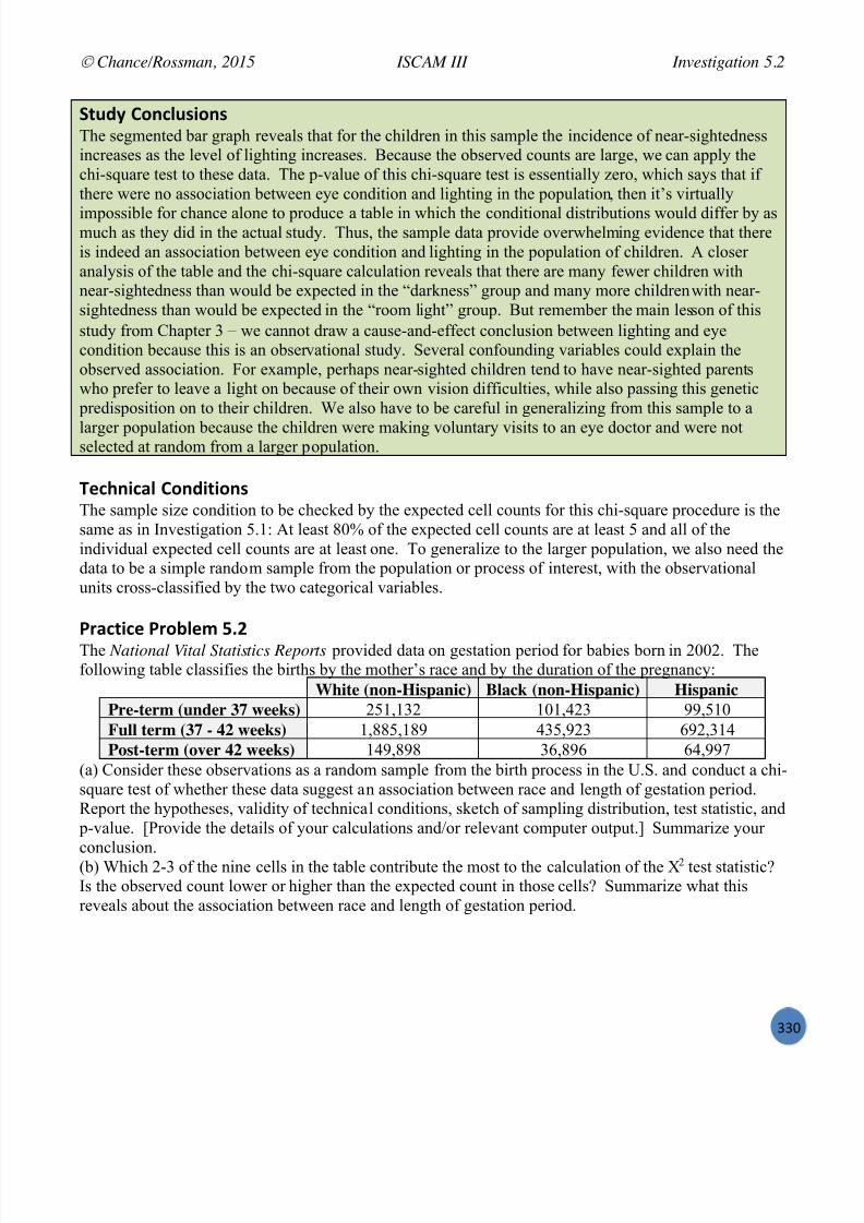
7/25/2019 Text: Investigating Statistical Concepts, Applications, and Methods
http://slidepdf.com/reader/full/text-investigating-statistical-concepts-applications-and-methods 331/428
Chance/Rossman, 2015 ISCAM III Investigation 5.2
##X
0+456 )'*7$4,8'*,The segmented bar graph reveals that for the children in this sample the incidence of near-sightednessincreases as the level of lighting increases. Because the observed counts are large, we can apply thechi-square test to these data. The p-value of this chi-square test is essentially zero, which says that ifthere were no association between eye condition and lighting in the population , then it’s virtually
impossible for chance alone to produce a table in which the conditional distributions would differ by asmuch as they did in the actual study. Thus, the sample data provide overwhelming evidence that thereis indeed an association between eye condition and lighting in the population of children. A closeranalysis of the table and the chi-square calculation reveals that there are many fewer children withnear-sightedness than would be expected in the “darkness” group and many more children with near-sightedness than would be expected in the “room light” group. But remember the main les son of thisstudy from Chapter 3 we cannot draw a cause-and-effect conclusion between lighting and eyecondition because this is an observational study. Several confounding variables could explain theobserved association. For example, perhaps near-sighted children tend to have near-sighted parentswho prefer to leave a light on because of their own vision difficulties, while also passing this genetic
predisposition on to their children. We also have to be careful in generalizing from this sample to a
larger population because the children were making voluntary visits to an eye doctor and were notselected at random from a larger population.
!%7=*87"$ )'*58+8'*,The sample size condition to be checked by the expected cell counts for this chi-square procedure is thesame as in Investigation 5.1: At least 80% of the expected cell counts are at least 5 and all of theindividual expected cell counts are at least one. To generalize to the larger population, we also need thedata to be a simple random sample from the population or process of interest, with the observationalunits cross-classified by the two categorical variables.
9:"7+87% 9:'#$%; VDRThe National Vital Statistics Reports provided data on gestation period for babies born in 2002. Thefollowing table classifies the births by the mother’s race and by the duration of the pregnancy:
White (non-Hispanic) Black (non-Hispanic) HispanicPre-term (under 37 weeks) 251,132 101,423 99,510Full term (37 - 42 weeks) 1,885,189 435,923 692,314Post-term (over 42 weeks) 149,898 36,896 64,997
(a) Consider these observations as a random sample from the birth process in the U.S. and conduct a chi-square test of whether these data suggest an association between race and length of gestation period.Report the hypotheses, validity of technical conditions, sketch of sampling distribution, test statistic, and
p-value. [Provide the details of your calculations and/or relevant computer output.] Summarize yourconclusion.(b) Which 2-3 of the nine cells in the table contribute the most to the calculation of the X 2 test statistic?Is the observed count lower or higher than the expected count in those cells? Summarize what thisreveals about the association between race and length of gestation period.

7/25/2019 Text: Investigating Statistical Concepts, Applications, and Methods
http://slidepdf.com/reader/full/text-investigating-statistical-concepts-applications-and-methods 332/428
Chance/Rossman, 2015 ISCAM III Investigation 5.2
##W
!%7=*'$'>6 /A?$':"+8'*I @"*5';8E"+8'* !%,+ (': )=8\,c4":% 0+"+8,+87What if our student involved random assignment rather than random sampling? How could we carry outa simulation analysis?
Suppose we wanted to analyze the Night Light study as a pseudo experiment and wanted to explore the
treatment effects of the lighting variable.(h) Outline the design of a simulation that will explore whether the association observed in our sampledata could plausibly have arisen from this random assignment process alone, using the chi-square teststatistic. [ Hint : Consider the data file with two columns, one for the response variable and one for theexplanatory variable.]
(i) Use technology to carry out this simulation. M* @I Create a function to store the chisq values (first initialize the vector), such as:01I6?9\ ! -GC3 &? ?< ,:,---* r
<;>3;G3BI7?C< ! 9B084;&3;G3BI7?C<*01I6?9\i?k – I6?9\=7;97&7BL4;&<;>3;G3BI7?C<Q 4?D67**W97B7?97?I
s M* B8*8+"#I Use the 5,95&)%'1./*%< worksheet and the %<1<&6/*&) macro. Remember to save
these files in the exact same folder (use quotations to force filename to end in mac). Use the Analyzing Two-way Tables applet. Copy and paste the two-way table (without totals and
using only one word variable names) into the Sample Data box and press Use Table . Make sure
the lighting condition is being used as the explanatory variable or press the (explanatory,response) button. Check the Show Shuffle Options box, enter a large number of shuffles, and press Shuffle . Use the pull-down menu to set the Statistic choice to the Chi-square ( 2) statistic.Check the box to Overlay Chi-square distribution. You can also check the Show 2 output boxto see the cell contributions.
(j) Does the randomization distribution appear to be well modeled by a chi-square distribution with df =4?
(k) Compute an empirical p-value based on the simulated chi-square values and compare it to the p-value calculated earlier. How do the p-values compare?
(l) If using R or Minitab, compute the p-value for each simulated chi-square value. M* @I Use '()&*)+'(A851= in your script M* B8*8+"#I Use Calc > Probability Distributions > Chi-Square and use your values (from
C20) in the Input column.Describe the shape, center, and variability of the distribution of these p-values. Explain why thisdistribution makes sense. [ Hint : Remember what assumption is behind the simulation.]

7/25/2019 Text: Investigating Statistical Concepts, Applications, and Methods
http://slidepdf.com/reader/full/text-investigating-statistical-concepts-applications-and-methods 333/428
Chance/Rossman, 2015 ISCAM III Investigation 5.2
##!
04;;":6 '( )=8\0c4":% !%,+ '( <,,'78"+8'*
Numerical and graphical summaries: conditional proportions and segmented bar graphs
If the data are a random sample from a larger population and the average expected cell count is at
least 5 (and all are at least 1) and you have classified each observational unit according to twocategorical variables, then the hypotheses:
H0: no association between variable 1 and variable 2 vs. H a: there is an association between variable 1 and variable 2
can be tested using the chi-square test statistic
r
i
c
j ij
ij ij
cted peex
cted peexobserved
1 1
22 .
The (upper-tail) p-value is calculated from thechi-square distribution with ( r 1)(c 1)degrees of freedom.
M* @ Create a matrix of the observed counts and use )+'(A/%,(%F*&%5'BG
To access the expected counts and (unsquared) chi-square contributions use)+'(A/%,(%F*&%5'BGe,B8,)%,; and )+'(A/%,(%F*&%5'BGe5,(';2&-(/
M* B8*8+"# Choose Stat > Tables > Chi-Square Test
for Association and specify the columnscontaining the table. Enter specify thecolumns with the two categoricalvariables or choose the Summarized dataoption and specify the columns containingthe table. Click OK .
Under Statistics, check the Chi-squaretest, expected cell counts, and each cell’scontribution to chi-square.
M* <*"$6E8*> !G'\G"6 !"#$%, "??$%+ You can paste in raw data or the two way table. Remember to use one word variable names
and categories. Check the Show Table and Show 2 output boxes.

7/25/2019 Text: Investigating Statistical Concepts, Applications, and Methods
http://slidepdf.com/reader/full/text-investigating-statistical-concepts-applications-and-methods 334/428
Chance/Rossman, 2015 ISCAM III Investigation 5.3
###
Investigation 5.3: Newspaper Credibility Decline
With the proliferation of the Internet and 24-hour cable news outlets, it has become much easier for people to hear much more information, much more quickly. However, this has led to speculation thatnews organizations attempt to convey information before it has been properly verified in an effort to
feed our impatience. USA Today reported that newspapers appear to be losing credibility over time(March, 2004). It cited a nationwide sample of 1,002 adults, 18 years or older, interviewed viatelephone (under the direction of Princeton Survey Research Associates) during the period May 6-16,2002. One of the questions asked was
O-,&(, 5&%, +1< *2)+ 612 %+'.> 612 )&. Mf\@fkf ,&)+ 153&.'K&%'1. 1. & ()&-, 19 P %1 W/ L. %+'( 9125point scale, “4” means you can believe all or most of what the organization says. “1” means you believ ,&-*1(% .1%+'.3 19 <+&% %+,6 (&6/ j1< <12-; 612 5&%, %+, =,-',4&='-'%6 19 F[f0E @IfC? [LI0If \@$IG 1.%+'( ()&-, 19 P %1 Wt
The interviewer then asked this question for several different news organizations (e.g., USA Today, NPR, MSNBC).
(a) Why is it important for the interviewer to rotate the list of organizations?
When asked about “The daily newspaper you are most familiar with,” the percentage distribution of the1002 responses in May, 2002 was:
Believe all oralmost all – 4 3 2
Believes almost nothing 1 Can’t Rate
20% 39% 25% 9% 7%
A similar study conducted in May, 1998 yielded the following results (981 responses).Believe – 4 3 2 Cannot Believe 1 Can’t Rate
27% 36% 24% 7% 6%
(b) Create a two-way table of counts to analyze the association between time and how people rate the believability of the daily newspaper they are most familiar with, among those who felt they could ratetheir daily newspaper. In other words, eliminate the “can’t rate” category from consideration. Alsoremember t o use the “explanatory variable” as the column variable and that the observed counts do needto be integers.

7/25/2019 Text: Investigating Statistical Concepts, Applications, and Methods
http://slidepdf.com/reader/full/text-investigating-statistical-concepts-applications-and-methods 335/428
Chance/Rossman, 2015 ISCAM III Investigation 5.3
##P
Discussion: If we have independent random samples from several populations as in Investigation 5.1, but the response variable has more than 2 categories ( r > 2), we can again extend the chi-square procedure. The expected counts and test statistic will be calculated exactly the same way as inInvestigation 5.2. The chi-square distribution with ( r 1) ! (c 1) degrees of freedom will be validwith the same technical condition on sample size and the null hypothesis is that the distributions of the
response variable are the same in all I populations. The alternative is that the I distributions are not allthe same.
You should notice that the mechanics are exactly the same whether you are testing homogeneity of proportions, comparing the distributions across several populations, or examining the association between two categorical variables. The difference lies in how the data were collected and therefore inthe scope of conclusions that can be drawn. In fact, these procedures are sometimes all phrased in termsof the association between variables, because this is mathematically equivalent to having the sameconditional distributions. Again, you need to consider the implications of whether or not the distributionof a variable was determined in advance by the researchers.
(c) State the null and alternative hypotheses, check the technical conditions, and carry out a chi-squaretest to assess whether the sample data provide strong evidence that the distribution of responses differs between the two years. State your conclusion in context.
)';?":8,'* +' +G'\,";?$% ! \+%,+If we collaps e the above table to focus on the “largely believable” (3 or 4) and “not largely believable”(1 or 2) breakdown, we obtain:
2002 sample 1998 sample TotalLargely believable 591 618 1209Not largely believable 341 304 645Total 932 922 1854
(d) Carry out a chi-square test to decide whether the difference in the population proportions giving alargely believable rating differed significantly between the two years.
(e) Now carry out a two-sided two-proportion z-test for this table. Report the test statistic and p-value.How do the p-values compare? What do you think is the relationship between the test statistics?

7/25/2019 Text: Investigating Statistical Concepts, Applications, and Methods
http://slidepdf.com/reader/full/text-investigating-statistical-concepts-applications-and-methods 336/428
Chance/Rossman, 2015 ISCAM III Investigation 5.3
##R
Discussion: The chi-square procedure can be used to compare two or more population proportions.When there are only two populations, the procedure is equivalent to a two-sided z-test for proportionsfrom Chapter 3. The chi-square statistic is equal to z2 and the chi-square p-value is equal to the two-sided p-value for the two-sample z-test. If the alternative hypothesis is two-sided, you can use either
procedure. If the alternative hypothesis is one-sided, then you should carry out the two-sample z-test to
obtain the one-sided p-value. If there are more than two populations, then you must use the chi-square procedure, which will only assess whether or not at least one population proportion differs from theothers.
For a 2 2 two- way table, another alternative is Fisher’s Exact Test as you learned in Chapter 3. It isalways appropriate to carry out Fisher’s Exact Test, though it may b e a bit less convenient with hugesample sizes (which becomes less of an issue with each new computer chip).
However, of all three of these procedures, the two-sample z-procedure is the only one that also enablesus to calculate a confidence interval to estimate the magnitude of the difference in the two population
proportions.
9:"7+87% 9:'#$%; VDT In February of 1993, NBC News admitted that it staged the explosion of a General Motors truck duringa segment of the program “Dateline NBC” in November of 19 92. The segment included crash footagethat explosively showed how the gas tanks of certain old GM trucks could catch fire in a sidewayscollision. In a nationwide poll of adults ( Times Mirror News Interest Index ) conducted in August, 1989,1507 respondents gave NBC news the following believability ratings.
Believe – 4 3 2 Cannot believe 1 Can’t rate32% 47% 14% 2% 5%
The same poll conducted Feb. 12-27, 1993 saw 2001 respondents give the following results:Believe – 4 3 2 Cannot believe 1 Can’t r ate
31% 42% 18% 6% 3%(a) Is the difference in believability ratings statistically significant between these two years? (Is this atest of homogeneity of proportions or a test of independence? Explain.)(b) Is this convincing evidence that the General Motors explosion caused a decrease in the believabilityof NBC News?

7/25/2019 Text: Investigating Statistical Concepts, Applications, and Methods
http://slidepdf.com/reader/full/text-investigating-statistical-concepts-applications-and-methods 337/428
Chance/Rossman, 2015 ISCAM III Section 5.1 Summary
##S
0%7+8'* VDH 04;;":6
This section introduced you to the chi-square test . You saw that this test arises in three differentsettings. One of these settings is comparing the proportions of success across two or more populations,when independent random samples are taken from the populations. Another setting is comparing the
entire distributions of a categorical response variable (which could include more than just twocategories) across two or more populations, again assuming independent random samples from each
population. The chi-square test in these two scenarios is testing homogeneity of proportions . The finalsetting to which the chi-square test applies is testing independence between two categorical variableswhen a random sample is drawn from a population and the observational units are classified accordingto two categorical variables.
You have found that the same chi-square test procedure applies to all of these settings. The test statisticis based on comparing observed counts in the two-way table to what counts would be expected if thenull hypothesis were true. You used simulation to investigate the sampling distribution of the chi-squaretest statistic, and studied the conditions under which that sampling/randomization distribution can be
well-approximated by the chi- squared probability distribution, providing an approximation of the test’s p-value. Finally, you learned that when the test indicates a statistically significant result, you can furtheranalyze the contributions of the individual cells in the table to the calculation of that test statistic to learnmore about the nature of the association. Example 5.1 presents an application of the chi-square
procedure.
7/25/2019 Text: Investigating Statistical Concepts, Applications, and Methods
http://slidepdf.com/reader/full/text-investigating-statistical-concepts-applications-and-methods 338/428
Chance/Rossman, 2015 ISCAM III Investigation 5.4
##T
SECTION 2: COMPARING SEVERAL POPULATION MEANS
In the previous section, you learned the chi-square test for comparing proportions among two or moregroups. One key point was that there are advantages to an overall procedure that compares theproportions simultaneously and controls the overall Type I error rate. When there are only two groups,this procedure was equivalent to the two-sided two-sample z -test for proportions. You will see a similarapproach in this section, addressing the issue of comparing two or more population means . Thetechnique you learn here will be used both for comparing population means based on independentrandom samples and also for assessing whether there is a treatment effect based on data from arandomized experiment.
Investigation 5.4: Disability Discrimination
The U.S. Vocational Rehabilitation Act of 1973 prohibited discrimination against people with physicaldisabilities. The act defined a disabled person as any individual who had a physical or mentalimpairment that limits t he person’s major life activities. In 1984, disabled individuals in the labor forcehad an unemployment rate of 7% compared to 4.5% in the non-impaired labor force.
Researchers conducted a study in the 1980s that examined whether physical disabilities af fect people’s perceptions of employment qualifications (Cesare, Tannenbaum, & Dalessio, 1990). The researchers prepared videotaped job interviews, using the same actors and script each time. The only difference wasthat the job applicant appeared with different disabilities:
No disability Leg amputation Crutches Hearing impairment Wheelchair confinement
Seventy undergraduate students were randomly assigned to view one of the videotapes, and they werethen asked to rate the candidate’s qualifications on a 1-10 scale. The research question is whethersubjects tend to evaluate qualifications differently depending on the applicant’s disability.
(a) Identify the observational units, explanatory variable, and response variable in this study. Identifyeach variable as quantitative or categorical. Is this an observational study or an experiment? Explain.
Observational units:
Explanatory: Type:
Response: Type:
Type of study:

7/25/2019 Text: Investigating Statistical Concepts, Applications, and Methods
http://slidepdf.com/reader/full/text-investigating-statistical-concepts-applications-and-methods 339/428
Chance/Rossman, 2015 ISCAM III Investigation 5.4
##U
(b) The mean applicant qualification scores for the five groups are amputee 4.429, crutches 5.921,hearing 4.050, none 4.900, and wheelchair 5.343. What additional pieces of information do you need inorder to decide whether these sample means are significantly different (more than you might expect bythe random assignment process alone)?
(c) State a null and an alternative hypothesis to reflect the researchers’ conjecture.
Null hypothesis:
Alternative hypothesis:
(d) Explain what a Type I error and a Type II error represent in this context.
Type I error:
Type II error:
(e) Consider the following sets of boxplots. What is the same and what is different about thedistributions displayed by these boxplots? In which group do you believe the evidence will be strongerthat at least one population mean differs from the others? Explain.
A: B:
Same:
Different:
Stronger evidence (A or B): Explain:

7/25/2019 Text: Investigating Statistical Concepts, Applications, and Methods
http://slidepdf.com/reader/full/text-investigating-statistical-concepts-applications-and-methods 340/428
Chance/Rossman, 2015 ISCAM III Investigation 5.4
##V
Discussion: In the above boxplots, the sample mean scores are roughly the same for graphs A and B(6.2, 4.4, 7.1, 3.1, 7.0)), but the variability within each group is much larger for the distributions in graphA. This larger amount of “within -sample” variation makes the difference s in sample means seem not asextreme compared to graph B. Graph B displays less within-sample variability and so the differences inthe sample means appear more extreme and provide more evidence that the crutches scores and the
hearing scores did not come from the same population with the same population mean. So, our goal incomparing the sample means will be to decide whether the differences in the sample means are largerthan what we would expect by random chance, where the amount of within-sample variation will give usan indication as how much we expect the response values to vary “by chance.”
(f) The actual data are stored in E'(&='-'%6f*8-16*,.%/ %B%. Produce parallel boxplots and descriptivestatistics of the qualification scores among the five groups. Record the descriptive statistics in the table
below.None Amputee Crutches Hearing Wheelchair
Sample sizeSample mean
Sample std. dev.
Do these data suggest evidence of a difference among the population means? Write a paragraphsupporting your statements.
Just as the chi-square test statistic provides a single number to compare how different sample
proportions are across several groups, we need a test statistic that simultaneously measures thedifferences in sample means among several groups. As noted above, we will do this by considering thevariation in the sample means from the overall mean, and assessing whether that variation is much largerthan would be expected based on the chance variation exhibited within the samples. (See the AppletExploration to explore another possible statistic.)
(g) What is the overall mean applicant qualification rating assigned by the 70 students?
(h) If we were to treat the five sample means as five observations, calculate the standard deviation ofthese five values. Then square the standard deviation to calculate the variance .
(i) Is it reasonable to allow each of these sample means to have the same relative contribution to ouroverall measure of variability between group means? Explain.

7/25/2019 Text: Investigating Statistical Concepts, Applications, and Methods
http://slidepdf.com/reader/full/text-investigating-statistical-concepts-applications-and-methods 341/428
Chance/Rossman, 2015 ISCAM III Investigation 5.4
#PX
Our measure of the variability between groups or “treatment effect” will be the weighted variance across the groups where the weights are the sample sizes.
(j) In this case, the sample sizes were equal to 14 in each group, so you can simply multiply your answerto (h) by 14 to measure the variability between groups:
Between-group variability =
In order to assess whether the sample group means vary enough to be considered statistically significant,we also need to consider the variability of qualification scores within each group. This will allow us todecide whether our deviations are larger than we would expect by chance. To take into accountinformation from all five groups, we will calculate the pooled variance across the groups (similar to
what was done in Investigation 3.5).
(k) Calculate the average variance across the five groups. [ Hint : Square each group’s standard deviationto obtain its variance, and then take the average of those five values.]
When the sample sizes are not equal, the more general formula for this pooled variance, weighted bysample size, is:
This provides an overall estimate of the “within -group” variability, which simplifies to the average ofthe group variances when the sample sizes are equal.
(l) In calculating a pooled variance, you are implicitly assuming that the variability is the same acrossthe groups. Explain how the sample statistics reveal that this is a reasonable belief for these data.
Our test statistic will consider the ratio of the variability between groups to the variability within groups.
(m) Calculate the ratio of your result from (j) divided by your result from (k).
(n) What is the smallest possible value that this ratio could ever assume? The largest?
15)()()()()( 2
552
442
332
222
11 x xn x xn x xn x xn x xn
.)1()1()1()1()1(
)1()1()1()1()1(54321
255
244
233
222
2112
nnnnnsnsnsnsnsns p
7/25/2019 Text: Investigating Statistical Concepts, Applications, and Methods
http://slidepdf.com/reader/full/text-investigating-statistical-concepts-applications-and-methods 342/428
Chance/Rossman, 2015 ISCAM III Investigation 5.4
#PW
(o) What types of values (large, small, positive, negative) will this ratio have when the null hypothesis isfalse, that is, when the population means are not all equal?
(p) Explain how we could simulate a randomization test to approximate the distribution of this teststatistic.
(q) Use technology to simulate such a randomization test by randomly assigning the 70 rating scores tothe five different disability groups (so that we are assuming no genuine treatment effect).
M* @I Modify the code used in Investigation 4.2. Remember to initialize the vector for storing thenew statistic. Use 7B8841 to keep track of group statistics. For example:. 0;B<9!7B8841&3B<AC0?d;AF9IC3;Q A?9BL?4?71Q 0;B<*. 9A9!7B8841&3B<AC0?d;AF9IC3;Q A?9BL?4?71Q 9A*
M* B8*8+"#I Use the PB<AC0%?9BL?4?71=0BI macro. M* +=% )';?":8*> N:'4?, Oa4"*+8+"+8F%P "??$%+I Copy and paste the raw data, being to clarify
which is the explanatory variable, and press Use Data . Check the Show Shuffle Options box,enter a larger number of shuffles, and press Shuffle Responses . Use the Statistic pull-downmenu to select the F-statistic .
(r) Calculate an empirical p-value for the ratio you calculated in (m). What conclusion would you draw based on this p-value?
Probability Result: For large samples, this sampling distribution is well modeled by an F distribution with parameters number of groups 1 and overall sample size number of groups , the degrees offreedom of the numerator and denominator respectively.

7/25/2019 Text: Investigating Statistical Concepts, Applications, and Methods
http://slidepdf.com/reader/full/text-investigating-statistical-concepts-applications-and-methods 343/428
Chance/Rossman, 2015 ISCAM III Investigation 5.4
#P!
!%:;8*'$'>6 2%+'4:We will compare I group means, where each group has n i observations. The overall sample sizewill be denoted by N = ni.
H0: There is no treatment effect or H 0: 1 = … = I Ha: There is a treatment effect or H a: at least one i differs from the rest
The between-group variability will be measured by looking at the sum of the squared deviationsof the group means to the overall mean, . Each group mean is weighted by the sample size ofthat group. We will refer to this quantity as the “sum of squares for treatment,” SST.
SST = I
iii x xn
1
2
We will then “average” these values by considering how many groups w ere involved. Thisquantity will be referred to as the “mean square for treatments.”
MST =)1( I
SST
Note, if we fix the overall mean, once we know I 1 of the group means, the value of the ith
mean is determined. So the degrees of freedom of this quantity is I 1.
The within-group variability will be measured by the pooled variance. In general, each term will be weighted by the sample size of that group. We will again divide by an indication of theoverall sample size across the group s. We will refer to this quantity as the “mean squares forerror,” MSE.
MSE = I N
sn I
iii
1
2)1( which has N I degrees of freedom.
The test statistic is then the ratio of these “mean square” quantities:
MSE MST
F
When the null hypothesis is true, this teststatistic should be close to 1. So larger valuesof F provide evidence against the nullhypothesis. The corresponding p-value comesfrom a probability distribution called the F distribution with I 1 and N I degrees offreedom.
We will use this F distribution to approximate both the sampling distribution of this test statisticin repeated samples from the same population (H 0: 1 = … = and the randomizationdistribution for a randomized experiment (H 0: no treatment effect) as long as the technicalconditions (see below) are met.Because we are focusing on the variance of group means, this procedure is termed Analysis ofVariance (ANOVA). With one explanatory variable, this is called one-way ANOVA.
x

7/25/2019 Text: Investigating Statistical Concepts, Applications, and Methods
http://slidepdf.com/reader/full/text-investigating-statistical-concepts-applications-and-methods 344/428
Chance/Rossman, 2015 ISCAM III Investigation 5.4
#P#
!%7=*'$'>6 2%+'4: – <3-J<
M* @ If you have the data in a response vector and an explanatory vector, you can use
(2**&56F&14F5,(81.(,q,B8-&.&%156GG
This will output the Mean Square values in the Mean Sq column, first for the treatment group (thedisability row) and then for the error term (Residuals).
M* B8*8+"# Choose Stat > ANOVA > One-Way . Enter Score as the response variable and
Disability as the Factor variable. Click OK .
Note: The “Response data are in a separatecolumn for each factor level” choice would beused if each sample occurred in its own column.Scroll up to see the ANOVA table, whichincludes the Mean Square column, first for thetreatment groups (the disability row) and thenfor the error term.
M* )';?":8*> N:'4?, Oa4"*+8+"+8F%P "??$%+ Paste data into Sample data box, being sure to clarify which is the explanatory variable. Press Use
Data . Check the Show ANOVA Table box.
(s) Verify that the F -statistic is then equal to the ratio of these two Mean Square values. Also verify thedf values (degrees of freedom) for each row. Report the p-value.
MST: MSE: F -statistic:
df numerator: df denominator:
p-value:

7/25/2019 Text: Investigating Statistical Concepts, Applications, and Methods
http://slidepdf.com/reader/full/text-investigating-statistical-concepts-applications-and-methods 345/428
Chance/Rossman, 2015 ISCAM III Investigation 5.4
#PP
!%7=*87"$ )'*58+8'*,There are several technical conditions required for this randomization distribution to be well modeled bythe F distribution: The distribution for each group comes from a normal population. The population standard deviation is the same for all the groups.
The observations are independent.When using this ANOVA F -test to compare several population means, we will check each condition asfollows: The normal probability plot (or dotplot or histogram) for each sample ’s responses is reasonably
well-behaved. The ratio of the largest standard deviation to the smallest standard deviation is at most 2. The samples are independent random samples from each population.
For simplicity, we will apply the same checks for a randomized experiment as well (with the lastcondition being met if the treatments are randomly assigned). If the first two conditions are not met,then suitable transformations may be useful.
(t) Is there evidence of non-normality in these sample data? Calculate the ratio of the largest to smalleststandard deviation; is this less than 2? (In the applet, check the box to Overlay F distribution to helpassess the fit.)
(u) Write a paragraph summarizing your conclusions for this study. Be sure to address issues ofcausation and generalizability as well as statistical significance.
0+456 )'*7$4,8'*,The distributions of qualification scores in the five treatment groups look reasonably symmetric withsimilar standard deviations, so it is appropriate to apply the Analysis of Variance procedure. There ismoderate evidence that the mean qualification ratings differ depending on the type of disability (p-value= 0.030). Descriptively, the candidates with crutches appear to have higher ratings on average, and thecandidates with hearing impairments tend to have slightly lower ratings. (Other follow-up procedurescould be used to determine which group means differ significantly from which others.) This was arandomized experiment, so we can attribute these differences in qualification scores to the disabilityshown. But we must be cautious about considering the students in this study to be representative of alarger population, particularly a population of employers who make actual hiring decisions.

7/25/2019 Text: Investigating Statistical Concepts, Applications, and Methods
http://slidepdf.com/reader/full/text-investigating-statistical-concepts-applications-and-methods 346/428
Chance/Rossman, 2015 ISCAM III Investigation 5.4
#PR
9:"7+87% 9:'#$%; VDU< Reconsider the boxplots from part (e). Explain how they compare and how this will affect thecalculation of the F -statistic and lead to different p-values. Explain based on how the F -statistic iscalculated which set of boxplots will have the smaller p-value.
9:"7+87% 9:'#$%; VDUCLifetimes of notable people in nine different occupational categories were gathered from The World
Almanac and Book of Facts .(a) How many different pairs of occupations can be considered?(b) Explain why conducting an ANOVA is different from conducting separate two-sample t -tests on all
possible pairs of occupations. Include an explanation for why it would be inappropriate to do all ofthose separate two-sample t -tests.(c) Would rejecting the null hypothesis in ANOVA allow you to conclude that every occupation beingstudied has a different population mean lifetime from every other occupation? Explain.
<??$%+ /A?$':"+8'*I @"*5';8E"+8'* !%,+ (': <3-J<
An alternative to using ANOVA for comparing a quantitative response variable across multiple groupsis to conduct a randomization test. As you have encountered with other scenarios, the randomizationtest involves
shuffling the observed values for one of the variables, say the response variable, recalculating the value of the statistic for the shuffled data, repeating that a large number of times to see the simulated null distribution of the statistic, and
then approximating a p-value based on where the observed value of the statistic falls in the simulated
null distribution.One advantage of the randomization test is that it can be performed on any reasonable statistic thatmeasures how much the response variable differs across the groups. You are no longer limited to usingthe ANOVA F -statistic, which might not have been the first statistic that would have occurred to you.
Reconsider the experiment from Investigation 5.4 about disability discrimination.
(a) State again the null hypothesis to be tested.
(b) Report again the sample mean qualification score for each group.Group None Amputee Crutches Hearing WheelchairSample mean
(c) Suggest a statistic for measuring how far apart these group means are. [ Hints : Your statistic should be a formula that produces a single number. Propose a statistic that is simpler and easier to calculatethan the F -statistic.]

7/25/2019 Text: Investigating Statistical Concepts, Applications, and Methods
http://slidepdf.com/reader/full/text-investigating-statistical-concepts-applications-and-methods 347/428
Chance/Rossman, 2015 ISCAM III Investigation 5.4
#PS
One simple but reasonable statistic is to calculate the average of all the absolute differences in samplemeans between pairs of groups. This statistic is called MAD (mean of absolute differences).
(d) How many pairs of groups are there in this study? [ Hint : Think combinations.]
(e) Why is it important to take the absolute values of the pairwise differences in group averages beforesumming them? [ Hint : Trying summing this without the absolute values.]
(f) Calculate the value of the MAD statistic for the disability discrimination.
After we calculate the value of the MAD statistic for the sample data, the next question is whether thisvalue is larger than would be expected by random chance if there were no treatment effect (i.e., if theresponse values would have turned out the same regardless of which explanatory group the person had
been assigned to). As we have done before in other situations, we can again investigate this question bysimulating the distribution of the MAD statistic under the null hypothesis.
(g) Open the Comparing Groups (Quantitative) applet to simulate anull distribution of these MAD statistics. Open theE'(&='-'%6f*8-16*,.%/%B% data file and paste the two columns (withcolumn names) into the applet; then press Use Data . Verify that thesample means agree with your answer to (a). Then report the valuethat the applet provides for the MAD statistic, and confirm that thismatches your answer to (f).
(h) Check the Show Shuffle Options box in the applet. Make sure that the radio button for the MADstatistic is checked. Press Shuffle Responses . Notice that the new dotplots and statistics are producedfor the shuffled data. Report the value of the MAD statistic for the shuffled data. Is this value moreextreme than the observed value of the MAD statistic from the experimental data? (How are youdeciding?)
(i) Press Shuffle Responses four more times. Record the four new values of the MAD statistic for theshuffled data. Are these all the same? Are any of them more extreme than the observed value of theMAD statistic from the experimental data?
(j) Now enter 995 for the Number of Shuffles and press Shuffle Responses , producing a total of 1000shuffles. Describe the shape of the null distribution of MAD statistic values. Is it symmetric or skewed?If it is skewed, in which direction is it skewed?
7/25/2019 Text: Investigating Statistical Concepts, Applications, and Methods
http://slidepdf.com/reader/full/text-investigating-statistical-concepts-applications-and-methods 348/428
Chance/Rossman, 2015 ISCAM III Exploration
#PT
(k) Is the null distribution centered at zero? Explain why your answer makes sense.
(l) In order to calculate an empirical p-value, you will count how many of the simulated MAD statisticsare equal to _______ or <larger or smaller>.
(m) In the Count Samples box enter the observed value of the MAD statistic and press Count . Reportthe empirical p-value.
(n) To obtain a more accurate approximation to the p-value, generate 9000 more random shuffles.Report the new empirical p-value.
(o) Interpret this p-value: It is the probability of obtaining a MAD statistic of ______ or ______,assuming that __________________________________________ .
(p) Based on the p-value, summarize the strength of evidence that the sample data provide against thenull hypothesis, in the context of this study. Also explain the reasoning process behind your conclusion.
The MAD statistic is fairly simple and intuitive, but it is not widely used. The F -statistic that youstudied earlier is far more commonly used, and the F -statistic has the advantage of taking into accountnot only the group means but also within-group variability. As a result, the F -statistic is more powerfulthan the MAD statistic.
(q) Explain what it means to say that the F -statistic is more powerful than the MAD statistic.
The applet conducts a randomization test based on the F -statistic as well as the MAD statistic.
(r) Use the pull-down Statistic menu to the F -statistic , and the null distribution changes from the MADstatistic to the F -statistic. Report the observed value of the F -statistic, which appears on the left side ofthe applet.
(s) Use the simulation results, and the observed value of the F -statistic, to determine an empirical p-value.

7/25/2019 Text: Investigating Statistical Concepts, Applications, and Methods
http://slidepdf.com/reader/full/text-investigating-statistical-concepts-applications-and-methods 349/428
Chance/Rossman, 2015 ISCAM III Exploration
#PU
(t) Check the box by Show ANOVA Table , and the applet reports more output including the p-value based on the F -distribution. Report this p-value. Is the empirical p-value from (s) close to thistheoretical p-value? Is the theoretical F -distribution, which is now overlaid on the simulated nulldistribution, a reasonable match?
(u) You have now calculated a p-value in three different ways, two using simulations of randomizationtests (with the MAD and F -statistics) methods and one based on the theoretical F -distribution. Are the
p-values all similar? Do they all lead to the same conclusion about the strength of evidence thathandicap type affects perception of qualification?
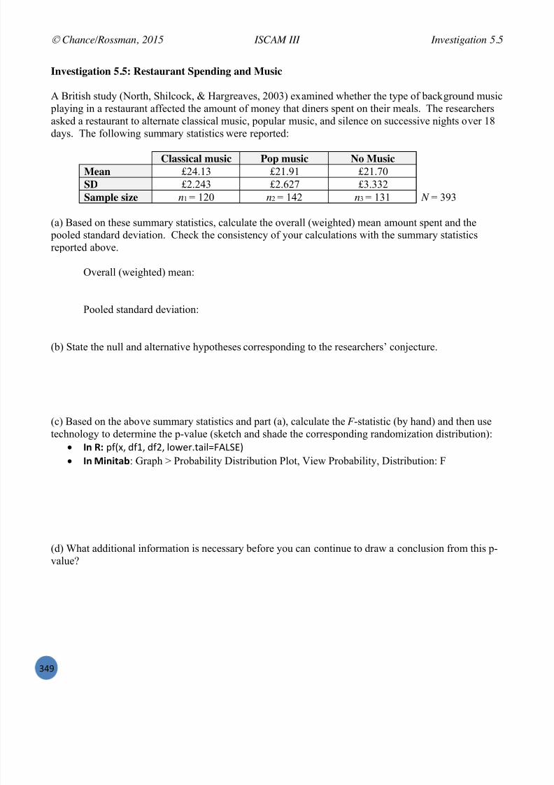
7/25/2019 Text: Investigating Statistical Concepts, Applications, and Methods
http://slidepdf.com/reader/full/text-investigating-statistical-concepts-applications-and-methods 350/428
Chance/Rossman, 2015 ISCAM III Investigation 5.5
#PV
Investigation 5.5: Restaurant Spending and Music
A British study (North, Shilcock, & Hargreaves, 2003) examined whether the type of background music playing in a restaurant affected the amount of money that diners spent on their meals. The researchersasked a restaurant to alternate classical music, popular music, and silence on successive nights over 18
days. The following summary statistics were reported:
Classical music Pop music No MusicMean £24.13 £21.91 £21.70SD £2.243 £2.627 £3.332Sample size n1 = 120 n2 = 142 n3 = 131 N = 393
(a) Based on these summary statistics, calculate the overall (weighted) mean amount spent and the pooled standard deviation. Check the consistency of your calculations with the summary statisticsreported above.
Overall (weighted) mean:
Pooled standard deviation:
(b) State the null and alternative hypotheses corresponding to the researchers’ conjecture.
(c) Based on the above summary statistics and part (a), calculate the F -statistic (by hand) and then usetechnology to determine the p-value (sketch and shade the corresponding randomization distribution):
M* @I 89FB7 ;9W7 ;9!7 -1<,5/%&'-_Q0\$fG M* B8*8+"#: Graph > Probability Distribution Plot, View Probability, Distribution: F
(d) What additional information is necessary before you can continue to draw a conclusion from this p-value?

7/25/2019 Text: Investigating Statistical Concepts, Applications, and Methods
http://slidepdf.com/reader/full/text-investigating-statistical-concepts-applications-and-methods 351/428
Chance/Rossman, 2015 ISCAM III Investigation 5.5
#RX
0+456 )'*7$4,8'*,In this study, a larger average amount was spent while classical music was playing. With such a largetest statistic and such a small p-value ( F = 31.48, p-value 0), we have very strong evidence that theobserved differences in the sample means could not have arisen by chance alone. However, we need toassess the technical conditions before we could know whether this inferential procedure is valid with
these data. Although the equal standard deviation assumption seems reasonable (because 3.332/2.243 <2), we do not have the sample data to examine the shapes of the sample distributions. Still, the samplesizes are large and the F procedure is fairly robust to departures from the normality condition. However,we should not consider these observations to be independent within each group, because the treatmentswere assigned to the evenings, not to the individual diners. In this sense, we only have a fewreplications per evening and ANOVA is not the appropriate analysis. Descriptively it appears that theaverage amount spent is larger when classical music is playing, but because of the confounding withevening, it’s possible that classical music was played on certain days of the week and that that lead tomore spending. This was a randomized experiment, so if it weren’t for the concern about independence,we would have been able to draw a cause-and-effect conclusion from the type of music played and theamount spent. We would want to be very cautious in generalizing these results to other restaurants and
even other times of the year.
<??$%+ /A?$':"+8'*I /A?$':8*> <3-J<
You will now explore the effects of such factors as the size of the difference in the population means,the overall population standard deviations, and the sample sizes on the F -test statistic and p-value.
Open the Simulating ANOVA Tables applet.The sliders and text boxes should specify:
23 as each population mean 120, 142, and 131 as the sample sizes 3 as the population standard deviation.
(e) Press the Draw Samples button. A sample will be selected from each population. What F -statisticand p-value did you obtain?
(f) Press the Draw Samples button again. Did you obtain the same F -statistic and p-value? Why not?
(g) Press the Draw Samples button 10-20 more times, watching how the boxplots, F , and p-valueschange. Did you ever obtain a p-value below 0.05? Is this possible? Would it be surprising? Explain.
7/25/2019 Text: Investigating Statistical Concepts, Applications, and Methods
http://slidepdf.com/reader/full/text-investigating-statistical-concepts-applications-and-methods 352/428
Chance/Rossman, 2015 ISCAM III Exploration
#RW
(h) Change the value of 1 to 24 . Press the Draw Samples button 10-20 times. Do the resulting p-values tend to be larger or smaller than in (g)? Explain why this makes sense.
(i) Change each of the sample sizes to 20 and press Draw Samples 10-20 times. Do the resulting p-values tend to be larger or smaller than in (h)? Explain why this makes sense.
(j) Press Draw Samples until you have a p-value < 0.3. Now change the value of to 7. (Drag theslider to decrease the value in increments of 0.1, or edit the orange value, watching how the p-valuechanges.) How does this affect the magnitude of the p-value? Explain why this relationship makessense.
(k) How does the p-value generally change if you now continue to increase the value of ? Explainwhy this relationship makes sense.
Discussion: If the null hypothesis is true, then the p-value should vary uniformly between 0 and 1. Inthis case, for example, the p-value will be less than 0.05 in 5% of all random samples, so 5% of samples
would you be led to reject the null hypothesis even when it is true. However, when there truly is adifference in the population means, our ability to detect that difference based on sample data is affected by several factors:
When the population means are further apart, the p-value is smaller. When the within-group variability is larger, the p-value is larger. When the sample sizes are larger, and there is a difference among the population means, then the p-value is smaller.

7/25/2019 Text: Investigating Statistical Concepts, Applications, and Methods
http://slidepdf.com/reader/full/text-investigating-statistical-concepts-applications-and-methods 353/428

7/25/2019 Text: Investigating Statistical Concepts, Applications, and Methods
http://slidepdf.com/reader/full/text-investigating-statistical-concepts-applications-and-methods 354/428
Chance/Rossman, 2015 ISCAM III Section 5.2 Summary
#R#
0%7+8'* VDR 04;;":6
Whereas the previous section dealt with comparing several groups on a categorical response variable,this one introduced you to comparing several groups on a quantitative response variable. You learnedhow to apply analysis of variance (ANOVA) to assess the significance of the differences among several
sample/treatment means. The test procedure is based upon a probability distribution known as the F -distribution. You have seen that the same ANOVA procedure applies whether the data were gathered asindependent random samples from several populations or from randomization of subjects to severaltreatment groups. (But like always, the scope of conclusions differs depending on how the data werecollected.) You have also found that ANOVA results are affected by the variability in sample means,the variability within samples/groups, and the sample sizes. Like always, you have examined technicalconditions that must be satisfied in order for this procedure to be valid; in addition to random samplingor random assignment, these conditions are that each group has a normal distribution and that thestandard deviations are similar across groups. Example 5.2 presents an application of the ANOVA
procedure.

7/25/2019 Text: Investigating Statistical Concepts, Applications, and Methods
http://slidepdf.com/reader/full/text-investigating-statistical-concepts-applications-and-methods 355/428
Chance/Rossman, 2015 ISCAM III Investigation 5.6
#RP
SECTION 3: RELATIONSHIPS BETWEEN QUANTITATIVE VARIABLES
In this section you will analyze data sets with two quantitative variables. The goal will be to describethe relationship between the variables. As always, you will start by learning some useful numerical andgraphical techniques for summarizing the data. Then you will explore how to use a mathematicalmodel of the relationship to make predictions of one variable from the other. In the next section you willthen move on to inferential techniques based on simulated sampling and randomization distributions aswell as a mathematical model.
Investigation 5.6: Cat Jumping Evolutionary biologists are often interested in “form -function relationships” to help explain evolutionhistory of say an animal species. Harris and Steudel (2002) investigated factors that are related to the
jumping ability of domestic cats. Because jump ability and height are largely dependent on takeoffvelocity, several traits were recorded for 18 healthy adult cats such as relative limb length, relativeextensor muscle mass, body mass, fat mass relative to lean body mass, and the percentage of fast-twitchmuscle fibers to see which might best explain maximum takeoff velocity (based on high-speed videos). Inthis investigation, you will examine the following data, also available in the file N&%c2*8'.3/%B%:
ID SexBody mass
(g)Hind limb
length (cm)Muscle mass
(g)Percentbody fat
Takeoff velocity(cm/sec)
A F 3640 29.1 51.15 29 334.5B F 2670 28.55 46.05 17 387.3C M 5600 31.74 95.9 31 410.8D F 4130 26.9 55.65 39 318.6E F 3020 26.11 57.2 15 368.7F F 2660 26.69 48.67 11 358.8G F 3240 26.74 64.55 21 344.6H M 5140 27.71 78.8 35 324.6I F 3690 25.47 54.6 33 301.4J F 3620 28.18 55.5 15 331.8K F 5310 28.45 68.8 42 312.6L M 5560 28.65 79.8 37 316.8M M 3970 29.82 69.4 20 375.6N F 3770 26.66 60.25 26 372.4O F 5100 27.84 60.7 41 314.3P F 2950 27.89 55.65 25 367.5Q M 7930 30.58 98.95 48 286.3R F 3550 28.06 79.25 16 352.5
(a) Identify the observational units and the primary response variable of interest here. Also classify thisvariable as quantitative or categorical.
Observational units:
Response variable: Type:

7/25/2019 Text: Investigating Statistical Concepts, Applications, and Methods
http://slidepdf.com/reader/full/text-investigating-statistical-concepts-applications-and-methods 356/428
Chance/Rossman, 2015 ISCAM III Investigation 5.6
#RR
(b) Open the N&%c2*8'.3/%B% data file and produce numerical and graphical summaries of the takeoffvelocity variable. Describe the distribution of takeoff velocities in this sample (shape, center, variability,unusual observations).
(c) Based on your analysis in (b), if you were going to randomly select a domestic cat, what is your best prediction of its takeoff velocity?
(d) Do you think there will be a relationship between a cat’s takeoff velocity and its body ma ss? If so,
do you think heavier cats will tend to have larger or smaller takeoff velocities than lighter cats?
We will need a new graphical summary to visually explore the relationship between two quantitativevariables, the scatterplot .
!%7=*'$'>6 2%+'4: – 07"++%:?$'+,
M* @. 84C7&LCA10B99Q H;4CI?71* or . 84C7&H;4CI?71pLCA10B99*. 9IB77;384C7&LCA10B99Q H;4CI?71* %+, ()&%%,58-1% 92.)%'1. '( '. %+, )&5 8&)>&3,
M* B8*8+"# Choose Graph > Scatterplot , with the Simple option. Click OK . Double click on velocity to enter this as the Y variable and then double click on bodymass to enter
this as the X variable. Click OK . [Or type NUe. 84C7 nH;4CI?71n+nLCA10B99n ]
(e) Describe the relationship between a cat’s takeoff velocity and its body mass, as displayed in thisscatterplot. Does this pattern confirm your expectation in (d)?

7/25/2019 Text: Investigating Statistical Concepts, Applications, and Methods
http://slidepdf.com/reader/full/text-investigating-statistical-concepts-applications-and-methods 357/428
Chance/Rossman, 2015 ISCAM III Investigation 5.6
#RS
(f) Do any of these cats appear to be outliers in the sense that its pair of values (body mass, takeoffvelocity) does not fit the pattern of the majority of cats? If so, identify the ID for that cat and describewhat’s different about this cat (in context).
!%:;8*'$'>6 2%+'4: Scatterplots are useful for displaying the relationship between two quantitative variables. If one variablehas been defined as the response variable and the other as the explanatory variable, we will put theresponse variable on the vertical axis and the explanatory variable along the horizontal axis.
In describing scatterplots you will describe the overall pattern between the two variables focusing primarily on three things:
Direction : Is there a positive association (small values of y tend to occur with small values of x andlarge values of y tend to occur with large values of x) or a negative association (small values of y tend to occur at large values of x and vice versa)?
Linearity : Is the overall pattern in the scatterplot linear or not? Strength : How closely are the observations following the observed pattern?
The above scatterplot reveals a fairly strong, negative association between body mass and takeoffvelocity, meaning that heavier cats tend to have a smaller takeoff velocity than larger cats. Therelationship is somewhat linear but has a bit of a curved pattern. There is one outlier cat (cat C) with avery high takeoff velocity despite having a very large body mass.
(g) Now produce a scatterplot of takeoff velocity vs. percentage of body fat. Describe the association.Would you say that the association with velocity is stronger than with body mass? More or less linear?
(h) For the other two variables (hind limb length and muscle mass), would you expect to see a positiveor negative association with takeoff velocity? Explain. Then look at scatterplots, and comment onwhether the association is as you expected.
7/25/2019 Text: Investigating Statistical Concepts, Applications, and Methods
http://slidepdf.com/reader/full/text-investigating-statistical-concepts-applications-and-methods 358/428
Chance/Rossman, 2015 ISCAM III Investigation 5.6
#RT
!%7=*'$'>6 2%+'4: – )'5%5 07"++%:?$'+,
M* @ Create the scatterplot as before, but pass a categorical variable as a color vector.
For example: . 84C7&H;4CI?71pLCA10B99Q IC4!9;[*
M* B8*8+"# Choose Graph > Scatterplot , with the “With Groups” option. Click OK . Enter the response and explanatory variables as before. Click in the Categorical variables box and enter the Sex column (e.g., double click on it in left
panel). Press OK .
(i) Now produce a coded scatterplot of takeoff velocity vs. body mass that uses different symbols formale and female cats (see Technology Detour above). Based on this graph, do you notice anydifferences between male and female cats with regard to these variables? Explain.
0+456 )'*7$4,8'*,These researchers reported that variation in cat maximum takeoff velocity was significantly explained
by both hind limb length (cats with longer limbs tended to have higher takeoff velocities) and fat massrelative to lean body mass (cats with lower fat mass tended to have higher takeoff velocities), but not toextensor muscle mass relative to lean mass or fast- twitch fiber content. They explained the “pervasive
effect” of body mass by the increase in muscle work invested in increasing the center of mass potentialenergy as compared with kinetic energy during takeoff.
Later in this chapter you will learn how they determined the statistical significance of theserelationships. First, we will examine a numerical measure of the strength of the association between twovariables.

7/25/2019 Text: Investigating Statistical Concepts, Applications, and Methods
http://slidepdf.com/reader/full/text-investigating-statistical-concepts-applications-and-methods 359/428
Chance/Rossman, 2015 ISCAM III Investigation 5.7
#RU
Investigation 5.7: Drive for Show, Putt for Dough
Some have cited “Drive for show, putt for dough” as the oldest cliché in golf. The message is that the best way to improve one’s scoring average in golf i s to focus on improving putting, as opposed to, say,distance off the initial drive, even though the latter usually garners more ooh’s and aah’s . To see
whether this philosophy has merit, we need to examine whether there is a relationship between puttingability and overall scoring, and whether that relationship is stronger than the relationship betweenscoring average and driving distance. The file 31-9,5(/%B% contains the 2004 statistics (through theHonda Classic on March 20) on the top 80 PGA golfers, downloaded fromhttp://www.pgatour.com/stats/ on March 20, 2004. Three of the variables recorded include: Scoring average : A weighted average which takes the stroke average of the field into account. It is
computed by adding a player’s total strokes to an adjustment, and dividing by the total rounds played. This average is subtracted from par to create an adjustment for each round. Keep in mindthat in golf low scores, as measured by number of strokes, are better than high scores.
Driving distance : Average number of yards per measured drive. These drives are measured on twoholes per round, carefully selected to face in opposite directions to counteract the effects of wind.
Drives are measured to the point where they come to rest, regardless of whether or not they hit thefairway. Putting average : On holes where the green is hit in regulation, the total number of putts is divided
by the total holes played.
(a) Do you expect the relationship between scoring average and driving distance to be positive ornegative? Explain.
(b) Do you expect the relationship between scoring average and putting average to be positive ornegative? Explain.
(c) Open the data file and examine a scatterplot of average score vs. driving distance and a scatterplot ofaverage score vs. average putts . Describe each scatterplot. Do the relationships confirm yourexpectations in (a) and (b)? Does one relationship appear to be stronger than the other? If so, which?

7/25/2019 Text: Investigating Statistical Concepts, Applications, and Methods
http://slidepdf.com/reader/full/text-investigating-statistical-concepts-applications-and-methods 360/428
Chance/Rossman, 2015 ISCAM III Investigation 5.7
#RV
To further analyze these data, we need a numerical way of measuring the strength of the association between the two variables. We will do this with the correlation coefficient .
The following are the above scatterplots with the x and y lines superimposed.
(d) For the average score vs. average putts scatterplot, in which quadrants are most of the points
located? For the average score vs. driving scatterplot? Which scatterplot seems to have fewer points inthe “non -aligned” quadrants?
Definition: A numerical measure of the strength of a linear relationship is the correlation coefficient , r .
n
i y
i
x
i
s y y
s x x
nr
111
where and s x are the mean and standard deviation of the explanatory variable, respectively, andand s y are the mean and standard deviation of the response variable.
Notice that when a point ( xi, yi) is in quadrant I or III, the term y y x x ii will be positive. When a point is in quadrant II or IV, this term is negative. Where there is a positive association, most of the points are in quadrants I and III, so the correlation coefficient is positive. Similarly, when there is anegative association, most of the points will be in quadrants II and IV, so the correlation coefficientturns out to be negative. The more observations that are in the “aligned” quadrants, and the closer the
points fall to a straight line, the larger the value of the correlation coefficient.
(e) Let x represent the average number of putts and y represent the average number of strokes. Use thedefinition of the correlation coefficient above to determine the measurement units of the correlationcoefficient r in terms of putts and strokes.
x y
III
III
III
IV III IV

7/25/2019 Text: Investigating Statistical Concepts, Applications, and Methods
http://slidepdf.com/reader/full/text-investigating-statistical-concepts-applications-and-methods 361/428
Chance/Rossman, 2015 ISCAM III Investigation 5.7
#SX
(f) If the correlation coefficient between two variables equals zero, what do you think the scatterplot willlook like?
(g) Suppose we find the correlation coefficient of a variable with itself. Substitute xi in for yi (and so x for y and s x for sy) in the above equation. Simplify. What is the correlation coefficient equal to?
(h) Do you think the correlation coefficient will be a resistant measure of association? Explain.
(i) The following scatterplots display 7 pairs of variables for these golfers. Rank these graphs in orderfrom strongest negative correlation to strongest positive correlation.A: B:
C: D:

7/25/2019 Text: Investigating Statistical Concepts, Applications, and Methods
http://slidepdf.com/reader/full/text-investigating-statistical-concepts-applications-and-methods 362/428
7/25/2019 Text: Investigating Statistical Concepts, Applications, and Methods
http://slidepdf.com/reader/full/text-investigating-statistical-concepts-applications-and-methods 363/428
Chance/Rossman, 2015 ISCAM III Investigation 5.7
#S!
(m) What does a correlation coefficient equal to zero signify?
(n) What does a correlation coefficient close to 1 or 1 signify?
(o) Which has a stronger correlation coefficient with scoring average: driving distance or average putts?Does this support the cliché? Explain.
0+456 )'*7$4,8'*, The correlation coefficient for scoring average and average putts indicates a moderately strong positivelinear association ( r = 0.444) whereas the correlation coefficient for scoring average and drivingindicates a weaker negative association ( r = 0 .265). This appears to support that putting performance ismore strongly related to a PGA golfer’s overall scoring average than the golfer’s driving distance, as thecliché would suggest. We must keep in mind that these data are only for only the first 2.5 months of theseason (when most golfers have played only around 6 – 8 events) and may not be representative of thescores and money earnings later in the year.
Discussion : The correlation coefficient, r , provides a measure of the strength and direction of the linear relationship between two variables. This is a unitless quantity which has the advantage that it will beinvariant to changes in scale (if we started looking at money in British pounds instead of Americandollars, our measure of the strength of the relationship will not change) or if we reverse which we callthe explanatory and response variables. A value of r close to zero indicates that the variables do nothave a strong linear relationship. However, this does not preclude them from having a very strong butnon-linear relationship. A scatterplot should be examined before interpreting the value of r . If therelationship is not linear, there are alternative measures of the strength of the association that can beused or the variables can be transformed and the transformed variables analyzed instead. If therelationship is linear, a correlation coefficient close to 1 or 1 indicates a very strong relationship. Thevalues of r form a continuum: as the linear association becomes weaker, the value of r becomes closer to
zero.
The correlation coefficient will always be a number between 1 and 1, inclusive. It will obtain the valueof 1 or 1 if the points fall along a perfect line (with negative or positive slope, respectively).

7/25/2019 Text: Investigating Statistical Concepts, Applications, and Methods
http://slidepdf.com/reader/full/text-investigating-statistical-concepts-applications-and-methods 364/428
Chance/Rossman, 2015 ISCAM III Exploration
#S#
<??$%+ /A?$':"+8'*I )'::%$"+8'* N4%,,8*> N";%
Open the Guess the Correlation applet. (a) Leave the number of points set to 25 and press
New Sample . The applet will display ascatterplot. Guess the value of the correlationcoefficient in this scatterplot and enter this guessinto the “Correlation guess” box . Then press theCheck Guess button.
How close was your guess? Were you surprised by the actual value? In what way? How mightyou guess differently the next time?
(b) Press the New Sample button, enter your guess for the value of the correlation coefficient for thisscatterplot, and press Enter . Describe how close you were and what adjustments you might make inyour thinking.
(c) Repeat this process for a total of 10 scatterplots (you do not need to record your results but youshould try to learn from the reveal of the actual values as you make your guesses). Do you think yourguessing ability improved by the last scatterplot? Explain.
(d) Check the Track Performance box. The first graph is “Guess vs. Actual” graph with the ( y = x) lineshown. Describe the behavior of the relationship between your guesses and the actual values of thecorrelation coefficients. Is there a strong correlation between your guesses and the actual values? Doesthis mean you are a good guesser? Explain.
(e) The next graph is the “Error vs. Actual” graph. Describe the behavior of the relationship betweenyour errors and the actual values of the correlation coefficients. Were some correlation coefficientseasier for you to guess than others? Use this graph to justify your answer.
7/25/2019 Text: Investigating Statistical Concepts, Applications, and Methods
http://slidepdf.com/reader/full/text-investigating-statistical-concepts-applications-and-methods 365/428
Chance/Rossman, 2015 ISCAM III Exploration
#SP
(f) The last graph is the “Error vs. Trial” graph. Describe the behavior of the relationship between yourerrors and the order in which you saw the graphs. Did your ability seem to improve over time? Use thisgraph to justify your answer.
(g) Suppose you guessed every value correctly; what would be the value of the correlation coefficient between your guesses and the actual correlations?
(h) Suppose each of your guesses was too high by 0.2 from the actual value of the correlationcoefficient. What would be the value of the correlation coefficient between your guesses and the actual
correlations?
(i) Does a correlation coefficient equal to 1 necessarily imply you are a good guesser? Explain.

7/25/2019 Text: Investigating Statistical Concepts, Applications, and Methods
http://slidepdf.com/reader/full/text-investigating-statistical-concepts-applications-and-methods 366/428
Chance/Rossman, 2015 ISCAM III Exploration
#SR
9:"7+87% 9:'#$%; VDZ<Suppose that we record the midterm exam score and the final exam score for every student in a class.What would the value of the correlation coefficient be if every student in the class scored:(a) Ten points higher on the final than on the midterm?(b) Five points lower on the final than on the midterm?
(c) Twice as many points on the final exam as on the midterm?Explain your answer in each part. [ Hint : You might first want to draw yourself a scatterplot ofhypothetical data that fit the stated conditions.]
9:"7+87% 9:'#$%; VDZC(a) The following scatterplots look at the relationships between house prices and four other variables.How does the strength of the linear relationship between price and square footage compare to thestrength of the relationships in the first 3 graphs?
(b) The correlations for these four graphs are0.284, 0.394, 0.649, 0.760
Which correlation coefficient do you think corresponds to which graph? Explain your reasoning.( Note : Each graph has the same number of houses, but you may have multiple houses indicated by anindividual dot.)
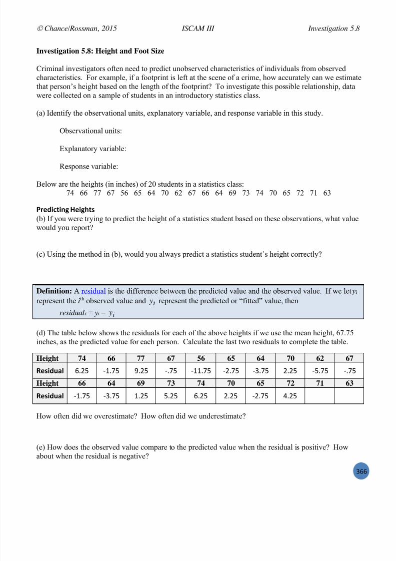
7/25/2019 Text: Investigating Statistical Concepts, Applications, and Methods
http://slidepdf.com/reader/full/text-investigating-statistical-concepts-applications-and-methods 367/428
Chance/Rossman, 2015 ISCAM III Investigation 5.8
#SS
Investigation 5.8: Height and Foot Size
Criminal investigators often need to predict unobserved characteristics of individuals from observedcharacteristics. For example, if a footprint is left at the scene of a crime, how accurately can we estimatethat person’s he ight based on the length of the footprint? To investigate this possible relationship, data
were collected on a sample of students in an introductory statistics class.
(a) Identify the observational units, explanatory variable, and response variable in this study.
Observational units:
Explanatory variable:
Response variable:
Below are the heights (in inches) of 20 students in a statistics class:
74 66 77 67 56 65 64 70 62 67 66 64 69 73 74 70 65 72 71 639:%587+8*> .%8>=+,(b) If you were trying to predict the height of a statistics student based on these observations, what valuewould you report?
(c) Using the method in (b), would you always predict a statistics student’s height correctly?
Definition: A residual is the difference between the predicted value and the observed value. If we let yi represent the ith observed value and i y
ˆ
repres ent the predicted or “fitted” value, then
residual i = yi – i yˆ
(d) The table below shows the residuals for each of the above heights if we use the mean height, 67.75inches, as the predicted value for each person. Calculate the last two residuals to complete the table.
Height 74 66 77 67 56 65 64 70 62 67
@%,854"$ S/!R :W/TR V/!R :/TR :WW/TR :!/TR :#/TR !/!R :R/TR :/TR
Height 66 64 69 73 74 70 65 72 71 63
@%,854"$ :W/TR :#/TR W/!R R/!R S/!R !/!R :!/TR P/!R
How often did we overestimate? How often did we underestimate?
(e) How does the observed value compare to the predicted value when the residual is positive? Howabout when the residual is negative?

7/25/2019 Text: Investigating Statistical Concepts, Applications, and Methods
http://slidepdf.com/reader/full/text-investigating-statistical-concepts-applications-and-methods 368/428
Chance/Rossman, 2015 ISCAM III Investigation 5.8
#ST
(f) How might you combine the residuals to measure the overall prediction error for these 20 students?
(g) Calculate the sum of the residuals from (d). Explain why taking the sum of residuals is not a useful
way to measure overall prediction error.
(h) Show mathematically that the sum of residual from the sample mean for any dataset equals zero. In
other words, show thatn
ii y y
1
)( = 0.
(i) Suggest two ways to get around the problem revealed in (g) and (h). In other words, suggestsomething related to but different from summing residuals to use as a useful measure of overall
prediction error.
(j) Suppose that you want to use a single number (call it m) for predicting height. Use calculus to
determine m, as a function of the data yi’s, to minimize the sum of squared residuals from that prediction. [ Hints : You are choosing m to minimize
n
ii m yS
1
2)( . Take the derivative with respect
to m, set it equal to zero, and solve for m.] Interpret your answer for m.
The Excel Exploration after this investigation asks you to consider minimizing other criteria, such as thesum of absolute residuals.

7/25/2019 Text: Investigating Statistical Concepts, Applications, and Methods
http://slidepdf.com/reader/full/text-investigating-statistical-concepts-applications-and-methods 369/428
Chance/Rossman, 2015 ISCAM III Investigation 5.8
#SU
9:%587+8*> .%8>=+, (:'; L''+$%*>+=, To see whether we can make better predictions of height by taking foot length into account, consider thefollowing scatterplot of the height (in inches) and foot length (in centimeters) for the sample of 20statistics students.
(k) Describe the association between height and foot length exhibited in this scatterplot. Is theassociation what you would have expected? Explain.
Open the Analyzing Two Quantitative Variables applet to see thescatterplot of the 20 students’ height and foot measurements . Check theShow Movable Line box to add a blue line to the scatterplot. The
equation for this initial line,
^
height = 67.75 + 0 foot size , predicts thesame height for all 20 students as you did in (d). (Note: the “hat” overheight indicates that the equation gives values for predicted height.)
If you now place your mouse over the green square on one of the ends of the line and drag, you canchange the slope of the line. You can also use the mouse to move the green square in the middle of theline up and down vertically to change the intercept of the line.
(l) Move the line until you feel your line “best” summarizes the relationship between height and foot
length for these data. Write down the final equation for your line. [ Hint : Use good statistical notation,which means to use variables names (not generic x and y) and to put a “hat” over the response v ariableto indicate prediction.]
(m) Did everyone in your class obtain the same line/equation?
r = .711

7/25/2019 Text: Investigating Statistical Concepts, Applications, and Methods
http://slidepdf.com/reader/full/text-investigating-statistical-concepts-applications-and-methods 370/428
Chance/Rossman, 2015 ISCAM III Investigation 5.8
#SV
(n) Does your line provide a better fit than your neighbor’s? Suggest a criterion for deciding which line“best” summarizes the relationship.
(o) Check the Show Residuals box to visually represent these residuals for your line on the scatterplot.The applet also reports the sum of the absolute residuals (or SAE, the sum of absolute errors). Recordthis SAE value for your line. What is the best SAE in the class? (Does “best” correspond to the smallestor the largest value of SAE?)
(p) A more common criterion for determining the “best” line is to instead look at the sum of the squared residuals (or sum of squared errors, SSE). Check the Show Squared Residuals box to visuallyrepresent them and to determine the SSE value for your line. What is the best SSE in the class?
(q) Continue to adjust your line until you think you have minimized the sum of the squared residuals.Report your new equation and new SSE value.
(r) Now check the Show Regression Line box to determine and display the equation for the line thatactually does produce the smallest possible sum of squared residuals. Report its equation and SSE value.Did everyone obtain the same line/equation this time? How does it compare to your line? (You can alsodisplay the residuals and the squared residuals for this line.)
Equation:
SSE:
Comparisons:
Definition : The line that minimizes the sum of squared residuals is called the least squares line , orsimply the regression line , or even the least squares regression line.
(s) Suggest a technique for determining (based on the observed data xi’s and yi’s) the values of the slopeand the intercept that minimize the SSE.

7/25/2019 Text: Investigating Statistical Concepts, Applications, and Methods
http://slidepdf.com/reader/full/text-investigating-statistical-concepts-applications-and-methods 371/428
Chance/Rossman, 2015 ISCAM III Investigation 5.8
#TX
K%",+ 0c4":%, @%>:%,,8'* K8*%I 2%:8F"+8'* '( )'%((878%*+,The least squares line y
ˆ
= b0 + b 1 x is determined by finding the values of the coefficients b0 and b1 that
minimize the sum of the squared residuals, SSE = ( yi - i yˆ
)2 =n
iioi xbb y
11 .
(t) Take the derivative with respect to b0 of the expression on the right. Then take the derivative of theoriginal expression with respect to b1. [ Hints : Use the chain rule, and remember to treat the data values
xi’s and yi’s as constants.]
(u) Set these (partial) derivatives equal to zero and solve simultaneously for the values of b0 and b1.[ Hints : Solve the first equation for b0. Then solve the second equation for b1 (substituting in theexpression for b0 using the summation notation).]

7/25/2019 Text: Investigating Statistical Concepts, Applications, and Methods
http://slidepdf.com/reader/full/text-investigating-statistical-concepts-applications-and-methods 372/428
Chance/Rossman, 2015 ISCAM III Investigation 5.8
#TW
You should have found expressions equivalent to the following.
n
xb yb
n
i
n
iii
1 11
0 and2
11
2
1 111
n
ii
n
ii
n
i
n
iii
n
iii
x xn
y x y xnb
With a little bit more algebra, you can show that the formulas for the least squares estimates of theintercept coefficient b0 and slope coefficient b1 simplify to:
b0 = y - b1 b1 = r s y/s x
(v) For the sample data on student s’ foot lengths ( x) and heights ( y), we can calculate these summarystatistics: = 28.5 cm, s x = 3.45 cm, y = 67.75 in and s y = 5.00 in, with r = 0.711. Use these statisticsand the formulas above to calculate the coefficients of the least-squares regression line. Confirm thatthese agree with what the applet reported for the equation of the least squares line.
(w) Use this least-squares regression line to predict the height of a person with a 28 cm foot length.Then repeat for a person with a 29-cm foot length. Calculate the difference in these two height
predictions. Does this value look familiar? Explain.
(x) Provide an interpretation of the slope coefficient ( b1) in this context.
(y) Provide an interpretation of the intercept coefficient ( b0) in this context. Is such an interpretationmeaningful for these data? Explain.
x
x

7/25/2019 Text: Investigating Statistical Concepts, Applications, and Methods
http://slidepdf.com/reader/full/text-investigating-statistical-concepts-applications-and-methods 373/428
Chance/Rossman, 2015 ISCAM III Investigation 5.8
#T!
Discussion: The slope coefficient of 1.03 indicates that the predicted height of a person increases by1.03 inches for each additional centimeter of foot length. In other words, i f one person’s foot length isone cm longer than another’s, we predict this person to be 1.03 inches taller than the other person.
Notice we are being careful to talk about the “ predicted ” change or “ average ” change, because these areestimates based on the least squares line, not an exact mathematical relationship between height and foot
length. The intercept coefficient can be interpreted as the predicted height for a person whose footlength is zero – not a very sensible prediction in this context. In fact, the intercept will often be too faroutside the range of x values for us to seriously consider its interpretation.
(z) Use the least squares regression line to predict the height of someone whose foot length is 44 cm.Explain why you should not be as comfortable making this prediction as the ones in (w).
Definition: Extrapolation refers to making predictions outside the range of the explanatory variablevalues in the data set used to determine the regression line. It is generally ill-advised.
/F"$4"+8*> +=% ;'5%$One way to assess the usefulness of this least-squares line is to measure the improvement in our
predictions by using the least-squares line instead of the y line that assumes no knowledge about theexplanatory variable.
(aa) In the applet, uncheck and recheck the Show Movable Line box. Check the Show SquaredResiduals box to determine the SSE if we were to use y as our predicted value for every x (foot size).Record this value.
SSE ( y ) =
(bb) Recall the SSE value for the regression line. Determine the percentage change in the SSE betweenthe y line and the regression line:
100% [(SSE ( y ) SSE (least-squares))/ SSE ( y )] =
Definition: The preceding expression indicates the reduction in the prediction errors from using the leastsquares line instead of the y line. This is referred to as the coefficient of determination , interpreted asthe percentage of the variability in the response variable that is explained by the least-squares regressionline with the explanatory variable. This provides us with a measure of how accurate our predictions will
be and is most useful for comparing different models (e.g., different choices of explanatory variable).The coefficient of determination is equal to the square of the correlation coefficient and so is denoted byr 2 or R2 (and is often pronounced “r -squared.”)
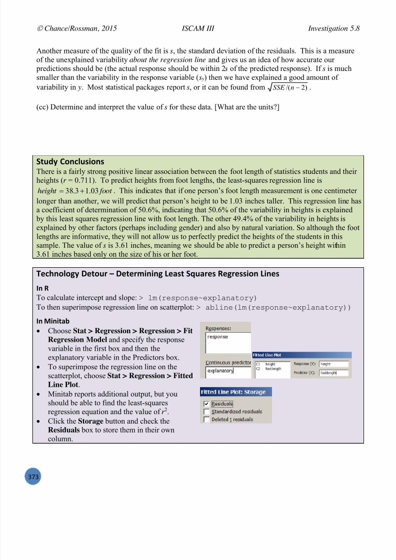
7/25/2019 Text: Investigating Statistical Concepts, Applications, and Methods
http://slidepdf.com/reader/full/text-investigating-statistical-concepts-applications-and-methods 374/428
Chance/Rossman, 2015 ISCAM III Investigation 5.8
#T#
Another measure of the quality of the fit is s, the standard deviation of the residuals. This is a measureof the unexplained variability about the regression line and gives us an idea of how accurate our
predictions should be (the actual response should be within 2 s of the predicted response). If s is muchsmaller than the variability in the response variable ( s y) then we have explained a good amount ofvariability in y. Most statistical packages report s, or it can be found from )2/( nSSE .
(cc) Determine and interpret the value of s for these data. [What are the units?]
0+456 )'*7$4,8'*, There is a fairly strong positive linear association between the foot length of statistics students and theirheights ( r = 0.711). To predict heights from foot lengths, the least-squares regression line is
foot eight h 03.13.38ˆ
. This indicates that if one person’s foot length measurement is one centimeterlonger than another, we will predict that person’s height to be 1.03 inches taller. This regression line hasa coefficient of determination of 50.6%, indicating that 50.6% of the variability in heights is explained
by this least squares regression line with foot length. The other 49.4% of the variability in heights isexplained by other factors (perhaps including gender) and also by natural variation. So although the footlengths are informative, they will not allow us to perfectly predict the heights of the students in thissample. The value of s is 3.61 inches, meaning we should be able to predict a person’s height wit hin3.61 inches based only on the size of his or her foot.
!%7=*'$'>6 2%+'4: – 2%+%:;8*8*> K%",+ 0c4":%, @%>:%,,8'* K8*%,
M* @To calculate intercept and slope: . 40&3;98C<9;p;[84B<B7C31*To then superimpose regression line on scatterplot: . BL4?<;&40&3;98C<9;p;[84B<B7C31**
M* B8*8+"# Choose Stat > Regression > Regression > Fit
Regression Model and specify the responsevariable in the first box and then theexplanatory variable in the Predictors box.
To superimpose the regression line on thescatterplot, choose Stat > Regression > FittedLine Plot .
Minitab reports additional output, but youshould be able to find the least-squaresregression equation and the value of r2.
Click the Storage button and check theResiduals box to store them in their owncolumn.

7/25/2019 Text: Investigating Statistical Concepts, Applications, and Methods
http://slidepdf.com/reader/full/text-investigating-statistical-concepts-applications-and-methods 375/428
Chance/Rossman, 2015 ISCAM III Investigation 5.8
#TP
9:"7+87% 9:'#$%; VD[For the Cat Jumping data set from Investigation 5.6:(a) Calculate and interpret the correlation coefficient between velocity and body mass.(b) Square the correlation coefficient to obtain r 2. Interpret the coefficient of determination in context.(c) Determine and interpret the slope of the least squares regression line.
(d) Determine and interpret the intercept of the least squares regression line. Explain what this valuemight signify in this context.(e) Determine and interpret the value of s.
<??$%+ /A?$':"+8'*I C%="F8': '( @%>:%,,8'* K8*%,
Open the Analyzing Two Quantitative Variables applet. Recall the 20 observations are height and footlength for a sample of statistics students.
(a) Check the Show Regression Line box. Does the regression line appear to do a reasonable job ofsummarizing the overall linear relationship in these data observations?
(b) If we were to add an observation with height 60 in and foot length 35 cm, predict whether, and if sohow, the regression line will change.
(c) Enter these coordinates in the Add/remove observations box ( x = 35, y = 60) and press the Add button. Report the new regression equation.
(d) Check the Move observations box. Click on this new observation (it should change color) and holdthe mouse button down and move the mouse vertically in both directions to change the y value of theobservation (try hard not to change the x value). The applet automatically recalculates the newregression line depending on the new location of the point. Is it possible to make the regression linehave a negative slope? Does the regression line appear to be affected by the location of this point? Isthe impact strong or weak? Does this match your prediction?
(e) Delete this new point and/or press the Revert button to return to the original data set. Now focus onthe point located at (29, 65). If we move this point vertically, predict how the regression line willchange. Do you think the change will be as dramatic as in (c)?

7/25/2019 Text: Investigating Statistical Concepts, Applications, and Methods
http://slidepdf.com/reader/full/text-investigating-statistical-concepts-applications-and-methods 376/428
Chance/Rossman, 2015 ISCAM III Exploration
#TR
(f) Repeat (d) using the point located at (29, 65). Does the regression line appear to be affected by thelocation of this point? Is the impact strong or weak (especially compared to the impact you witnessed in(d))?
(g) Which point was more influential on the equation of the regression line: (35, 60) or (29, 65)?Suggest an explanation for why the point you identified is more influential, keeping in mind the “least -squares crit erion.”
/A7%$ /A?$':"+8'*I B8*8;8E"+8'* ):8+%:8"
Another way to get around the problem revealed in (g) and (h) of Investigation 5.8, that the sum ofresiduals from the mean always equals zero, is to examine the sum of the absolute deviations.
(a) Using your results in the table in question (d) of Investigation 5.8, calculate the sum of the absolutevalues of the residuals, using the mean height as the predicted value.
Let’s investigate whether there is a better number (call it m) than the mean to use for predicting height,in order to minimize our prediction errors. In general, this sum of absolute residuals (or SAE, sum of
absolute errors) can be written: n
ii m ySAE
1
The problem with using the SAE is that it is not easily differentiable, so we cannot use calculus todetermine the optimal value for m. Instead, we will use Excel to explore the behavior of SAE as afunction of m. We will look for the value of m that minimizes SAE.
(b) Open the Excel spreadsheet document T;?D679=[49 . Notice that the 20 heights are in column A(sorted), and column B contains candidates for m from 65 to 70, in increments of 0.01. Click on cell C2,and notice that it contains a formula for SAE( m), which refers to the data values in column A and to thevalue of m from B2 (namely, m = 65 in that cell). Use Excel’s “fill down” featur e to calculate the valuesof SAE( m) for the remainder of column C. [ Hint : You can do this in one of several ways: With the C2cell selected, double click on the box in the lower right corner, or pull the right corner of the highlightedC2 cell down to the end of the column, or highlight C2 and the cells to be filled and choose Edit> Fill>Down.] Confirm that the SAE value for the sample mean (67.75) agrees with what you calculated in (a).

7/25/2019 Text: Investigating Statistical Concepts, Applications, and Methods
http://slidepdf.com/reader/full/text-investigating-statistical-concepts-applications-and-methods 377/428
Chance/Rossman, 2015 ISCAM III Exploration
#TS
(c) To produce a graph of SAE as a function ofm: Highlight columns B and C. Choose Insert >Scatter and then choose the first option in thesecond row (Scatter with Smooth Lines) toconstruct a graph of this function.
[ Hint : After you create the graph, you may wantto change the x-min and x-max values by doubleclicking on the horizontal axis and changing theMinimum and Maximum under Axis Options.]
Reproduce a rough sketch of this graph below, and comment on the shape of this function. Does it seemto follow a familiar form, such as linear or parabolic or exponential? Explain.
(d) Does there seem to be a unique value of m that minimizes this SAE( m) function? If so, identify it. Ifnot, describe all values of m that minimize the function. Also report the value of the SAE for thisoptimal value of m. [ Hint : Search through the entries in column C to find the smallest value, and thenread off the corresponding value in column B.]
Optimal m = SAE at the optimal m =
(e) Look through the sorted heights in column A. What do you notice about where this optimal value ofm is located in the list of sorted heights? Does this remind you of a familiar statistic?
(f) Suppose the tenth largest height (in row 11) had been 66 inches instead of 67. Make this change tothe spreadsheet (cell A11), and note that the graph of the SAE function is updated automatically. Nowis there a unique value of m that minimizes this SAE( m) function? If so, identify it. If not, describe allvalues of m that minimize the function, and also report the (optimal, minimum) value of the SAE.
Optimal m = SAE at the optimal m =
(g) Return the tenth largest height back to 67 inches. Now suppose the tallest person in the sample had been 80 inches tall instead of 77. Make this change to the spreadsheet (cellA21) and note how the graphof the SAE function changes. Also report the value of the SAE.
Optimal m = SAE at the optimal m =

7/25/2019 Text: Investigating Statistical Concepts, Applications, and Methods
http://slidepdf.com/reader/full/text-investigating-statistical-concepts-applications-and-methods 378/428
Chance/Rossman, 2015 ISCAM III Exploration
#TT
(h) Based on these findings, make a conjecture as to how one can determine, from a generic set of 20data values, the value that minimizes the sum of the absolute prediction errors from the data values.
(i) Consider a new minimization criterion: mean absolute error (MAE) criterion, which divides the SAEvalue by the number of observations. How would the MAE( m) function compare to the SAE( m)function? Would its minimum be achieved at the same value(s) of m? Explain.
Discussion : You should have found that the SAE function is piecewise linear . In other words, thefunction itself is not linear, but its component pieces are linear. In this case the function changes itsslope precisely at the data values. The SAE function (and MAE function) are minimized at the median
of the data and also at any value between (and including) the two middle values in the dataset (the 10th
and 11 th values in this case with n = 20 values). It is a convenient convention to define the median as theaverage (midpoint) of those two middle values. The MAE has a bit more natural interpretation – theaverage deviation of the values in the data set from the value of m.
Another criterion is to find the value of m that minimizes the sum of the squared deviations .
(j) Recall from (j) of Investigation 5.8 the value of m that minimizes the sum of the squared predictionerrors. Report this value of m for the height data.
(k) Make sure that the data values in column A are back to their original values. Then click on cell D2in the Excel spreadsheet, and notice that it gives the formula for the SSE (sum of squared errors)function. Fill this formula down the column and create a second graph to display the behavior of thisfunction. [ Hints : Click on column B and then hold the mouse down when you click on column D toheight just those two columns before you insert the graph. You will probably want to double click on the
y-axis scale to change its minimum value.] Does this function have a recognizable form, such as a polynomial? What is its shape? At what value of m is the function minimized? Does this value lookfamiliar?
(l) Suppose there had been a clerical error in entering the height of the tallest student. Change the heightof the tallest student from 77 inches to 770 and investigate the effect on the SSE function. Has the valueof m that minimizes SSE changed? By how much? How does this compare to the effect of this clericalerror on the SAE function and where it is minimized?

7/25/2019 Text: Investigating Statistical Concepts, Applications, and Methods
http://slidepdf.com/reader/full/text-investigating-statistical-concepts-applications-and-methods 379/428
Chance/Rossman, 2015 ISCAM III Exploration
#TU
Discussion: Although the SAE criteria would be more resistant to outliers, it does not always lead to aunique minimum (e.g., an even number of data values where the values of the middle pair are not equal).This has led to the more common criterion of least squares .
See the exercises for investigating additional minimization criteria, such as the median of absolute errors
and maximum of absolute errors.
Investigation 5.9: Money-Making Movies
Is there a tendency for movies that garner better reviews to also earn more money at the box office?USA Today (Wloszczyna & DeBarros, Feb. 25, 2004) investigated this by determining a rating score formovies released in 2003 based on a compilation of movie reviews published in 20 major newspapers andmagazines for over 300 movies. The *14',(X#/%B% data file contains these scores and how much moneythe movie made at the box office, in millions of dollars. A high composite score indicates that mostcritics loved the movie, and a low score indicates that most critics panned the movie.
(a) Identify the observational units in this study. Also identify the explanatory and response variables,and classify them as categorical or quantitative.
Observational units:
Explanatory:
Response:
(b) Produce a scatterplot to determine whether the critic scores appear to help predict the box office
gross. Describe the relationship between the two variables as exhibited in the scatterplot.
(c) Identify the two or three points that you believe have the largest (in absolute value) residuals. Identifythese movies by name
M* @I You can use a command like . 0CH?;9-(i9IC3; . b- l LC[=CGG?I; . #_-Q k M* B8*8+"#I Use the “brush” feature: Editor > Brush , and then Editor > Set ID variables
What does it mean for these movies to have such large residuals?

7/25/2019 Text: Investigating Statistical Concepts, Applications, and Methods
http://slidepdf.com/reader/full/text-investigating-statistical-concepts-applications-and-methods 380/428
Chance/Rossman, 2015 ISCAM III Investigation 5.9
#TV
(d) Determine, report, and interpret the value of the correlation coefficient.
(e) Use technology to determine the least squares regression line for predicting the box office gross fromthe composite critics’ score. Report the equation for th is line. Also interpret the slope and intercept ofthis line in context.
Equation of line:
Interpretation of slope:
Interpretation of intercept:
(f) Report the value of r2 and s provide interpretations in this context.
!%7=*'$'>6 2%+'4: – ):%"+8*> " )'5%5 07"++%:?$'+ G8+= 0%?":"+% K8*%,
M* @ Create the coded scatterplot: . 84C7&LC[=CGG?I;p9IC3;Q IC4!3B7?<D* Add the separate lines for each category, e.g.,:
. BL4?<;&40&LC[=CGG?I;i3B7?<D!!5o5kp9IC3;i3B7?<D!!5o5k**To cycle through the categories, create a column for the four categories and create a loop:. ICA;!I&5o5Q 5fo5Q 5fo),(5Q 5P5*. GC3 &? ?< ,:]*r
BL4?<;&40&LC[=CGG?I;i3B7?<D!!ICA;i?kkp9IC3;i3B7?<D!!ICA;i?kk*QIC4!?* s
To add a legend: . 4;D;<A&57C84;G75Q 4;D;<A!ICA;Q IC4!,:]Q 8I6!,*
M* B8*8+"#
Choose Graph > Scatterplot and choose the With Groups option. Enter the box office values and the ratings for the movies as before. In the Categorical variables box enter the “rating” variable (PG -13 etc.) and then click the box next to
“X-Y pairs from groups.” The resulting scatterplot should have the movies coded by rating. Right click on the scatterplot and choose Add > Regression Fit . Check the box to Apply same
groups … . Click OK .

7/25/2019 Text: Investigating Statistical Concepts, Applications, and Methods
http://slidepdf.com/reader/full/text-investigating-statistical-concepts-applications-and-methods 381/428
Chance/Rossman, 2015 ISCAM III Investigation 5.9
#UX
(g) Describe what this coded scatterplot reveals about whether the relationship between box officeincome and critic scores differs across the various rating categories. In particular, does any ratingcategory tend to have higher box office values than you would expect for the score they received fromthe critics? Is there a rating category tending toward lower box office revenues than expected? Explain.
(h) Repeat (g) using the movie genre (e.g., comedy) as the categorical variable.
(i) In analyzing these movies, the researchers also looked at the data set after removing the 6 movies thatearned more than $200 million. Subset the data (e.g., Investigation 2.1) and then examine the
scatterplot, correlation coefficient, and least-squares regression line for predicting the movie revenuefrom the critics’ rating score for these data.
New correlation coefficient: New least-squares regression line:
(j) Describe the effect of removing these 6 movies from the analysis.
Definition: An observation or set of observations is considered influential if removing the observationfrom the data set substantially changes the values of the correlation coefficient and/or the least squaresregression equation. Typically, observations that have extreme explanatory variable outcomes (far
below or far above ) are potentially influential. To measure the influence of an observation, it isremoved, and measures are calculated for how much the summary results change. It is not always thecase that the points with the largest residuals are the most influential.In this example you should have seen that removing those six movies actually makes the relationship
between box office income and critic scores much weaker ( r drops from 0.42 to about 0.3).
0+456 )'*7$4,8'*,
There does appear to be a weak relationship between the composite critics’ sco res and the amount ofmoney the movie makes at the box office, with higher rated movies making more money. If thecomposite critics’ score is 10 points higher, we predict the movie will make about 18.57 million moredollars. It is interesting to note that this regression line will tend to overestimate the amount of revenuefor an R rated movie and underestimate the revenue of action movies. If the top 6 grossing movies of2003 ( Bruce Almighty, Finding Nemo, Pirates of the Caribbean, The Lord of the Rings III, The Matrix
Reloaded, and X2: X-Men United ) are removed, the relationship is not as strong, but still shows a weak positive linear association ( r = 0.3).
x

7/25/2019 Text: Investigating Statistical Concepts, Applications, and Methods
http://slidepdf.com/reader/full/text-investigating-statistical-concepts-applications-and-methods 382/428
Chance/Rossman, 2015 ISCAM III Investigation 5.9
#UW
9:"7+87% 9:'#$%; VD](a) Which do you think will be more resistant to outliers, the regression line that minimizes the sum ofsquared errors or the regression line that minimizes the sum of the absolute errors? Explain.(b) Investigate your conjecture using the Analyzing Two Quantitative Variables applet. Write a short
paragraph summarizing your analysis and your observations.
0%7+8'* VDT 04;;":6
In this section you considered the association between two quantitative variables. Because this was yourfirst encounter with this type of analysis scenario, we returned to several themes from Chapter 1,including starting with graphical displays and numerical summaries. You learned that the relevantgraphical display for describing the association between two quantitative variables is a scatterplot , andthat some features to look for in a scatterplot are the direction , strength , and linearity of the association.The most common numerical summary of a linear association is the correlation coefficient , and youstudied some properties of this measure. Then you turned your attention to fitting a linear model to thedata, useful for predicting the value of the response variable based on an explanatory variable outcome.You studied the least squares criterion for determining this regression line and derived the equations forestimating the coefficients from sample data. With the regression line in hand, you can make
predictions for the response variable outcome based on the explanatory variable value. Just keep inmind that these predictions should be made only for x values within the range of the original data (andnot extrapolating beyond the original explanatory variable values. Finally, you examined properties ofregression lines, such as the coefficient of determination , which reveals how much of the variability inthe response variable is explained by the regression line, and influential observations , which havesubstantial effect on the regression line and typically arise from observations with extreme explanatoryvariable values.

7/25/2019 Text: Investigating Statistical Concepts, Applications, and Methods
http://slidepdf.com/reader/full/text-investigating-statistical-concepts-applications-and-methods 383/428
Chance/Rossman, 2015 ISCAM III Investigation 5.10
#U!
SECTION 4: INFERENCE FOR REGRESSION
In the previous section you learned graphical and numerical techniques for describing the relationshipbetween two quantitative variables, namely scatterplots and correlation coefficients. You also learned amethod for fitting a linear model to predict the value of one quantitative variable from another. But youonly described sample data in the previous section. In this section, you will again make the transition toinference : what can we conclude about a larger population or about the statistical significance of theassociation based on the sample results?
Investigation 5.10: Running Out of TimeMany communities offer racing events for amateur runners, such as 5K (approximately 3.1 miles) races.At the end of the event, awards are often given out to runners with the fastest times, often to the top threefinishers in different age groups. But does running time really change with age for amateur runners? Toinvestigate this, one of the authors downloaded the race results for a local 5K race in May 2013(I&--,6Ru!XW#/%B%). Data for 248 runners included age (in years) and finish time (in minutes).
(a) Identify the explanatory and response variables for this research question.
EV: RV:
(b) Do you expect the relationship between finish time and age to be positive or negative? Do you expectit to be linear (which implies what)? Do you think the association between these variables will bestatistically significant?
Direction:
Form:
Significance:
(c) Use technology to produce a scatterplot of finish time vs. age . [You can copy the data into Excel,using Data > Text to Columns and then delimiting by spaces, and then copy the last two columns (age,time in that order) into the Analyzing Two Quantitative variables applet.] Do you want to change any ofyour answers to (b) in light of this graph? Also discuss any other unusual features of the data.
(d) Remove the outlier (the name was a duplicate and the time was later dropped from the official
published results), and determine the least-squares regression equation for predicting finish time fromage. Interpret the slope coefficient in context.

7/25/2019 Text: Investigating Statistical Concepts, Applications, and Methods
http://slidepdf.com/reader/full/text-investigating-statistical-concepts-applications-and-methods 384/428
Chance/Rossman, 2015 ISCAM III Investigation 5.10
#U#
(e) Suppose we consider the remaining 247 runners to be a random sample from some larger population.Is it possible that there is no association between age and finishing time in this larger population, but we
just happened to find such an association in this sample? How might we investigate how plausible thisexplanation is?
!%:;8*'$'>6 2%+'4:To differentiate between the population regression line and the sample regression line, we will continueto use b0 and b1 to denote the sample statistics for the intercept and slope, respectively (or alternatively
ˆ
0 and ˆ
1). The corresponding population parameters will be denoted by 0 and 1.
(f) If there were no relationship between height and age in the population, what would this imply aboutthe value of the population slope? State null and alternative hypotheses to reflect the research questionthat 5K runner finishing times change with age. (Do you think they will increase or decrease?)
We now want to access the statistical significance of the association between variables in this sample.Following our usual logic, we will approach this question by assessing how unusual it would be to obtaina sample slope coefficient of b1 = 0.140 (or more extreme) with a random sample of 247 runners from a
population with no association between the variables (i.e., with a population slope coefficient of = 0).We will do this by creating such a population and repeatedly taking random samples from it, calculatingthe sample slope each time.
First, let’s think about what we want this population to look like.
(g) Determine the sample mean and standard deviation of the remaining individual variables in oursample:
Finish time Mean = Standard deviation =
Age Mean = Standard deviation =
Also determine the value of s from the regression model ( )2/( nSSE ) in (d) =
So one approach is to create a population that has similar characteristics as this sample, but with a population slope coefficient of zero.Technical note : You also want think about whether you want to model random sampling from a
bivariate population, or random sampling of finishing times at each age. We will start with the firstapproach, but classical regression theory (Investigation 5.12) assumes the second.

7/25/2019 Text: Investigating Statistical Concepts, Applications, and Methods
http://slidepdf.com/reader/full/text-investigating-statistical-concepts-applications-and-methods 385/428
Chance/Rossman, 2015 ISCAM III Investigation 5.10
#UP
In the Analyzing Two Quantitative Variables applet, check the Create Population box in the bottomleft corner. We will create a population of runners where there is no relationship between finish time andage . To match the above context: Set the population intercept to be equal to the mean
of the time variable, 32.36 . Because we are forcing
0, this says that the population regression line isconstant at y = 32.36 minutes. Set the x mean and x standard deviation to match
the values you found in (g) for age after removing theoutlier.
Set the value of sigma , representing the variabilityabout the population regression line, to equal thevalue of s from the regression model (should besmaller than the SD(Y) you found in (g)).
Press the Create Population button. Press Rescale .
Note: These values should appear in theapplet when you check Create Populationif you had pasted in the sample data first.
So the population of 20,000 runners we are creating here matches the characteristics of the observedsample data. The key difference here is that we are assuming the population slope is equal to zero.
(h) Check the Show Sampling Options box and set the sample size to be 247 and press the DrawSamples button. Did you obtain the same sample regression line (in blue) as from the observed raceresults or as in the hypothesized population (in red)?
(i) Press the Draw Samples button again. Make sure Show Regression Line is checked and record theregression line displayed in blue. Did you obtain the same sample regression line as in (h)?
Discussion : These questions reveal once again the omnipresent phenomenon of sampling variability .Just as you have seen that the value of a sample mean varies from sample to sample, the value of asample proportion varies from sample to sample, and the value of a chi-square statistic varies fromsample to sample, now you see that the value of a sample regression line also varies from sample tosample. Once again we can use simulation to explore the long-run pattern of this variation,approximating the sampling distributions of the sample slope coefficients and the sample interceptcoefficients.
(j) Change the Number of Samples from 1 to 20. Press the Draw Samples button. Describe the
pattern of variation that you see in the simulated regression lines.
(k) Now change the number of samples to 1000 and press the Draw Samples button. On the next page,describe the shape, mean, and standard deviation of this distribution.
7/25/2019 Text: Investigating Statistical Concepts, Applications, and Methods
http://slidepdf.com/reader/full/text-investigating-statistical-concepts-applications-and-methods 386/428
Chance/Rossman, 2015 ISCAM III Investigation 5.10
#UR
Shape:
Mean: Standard deviation:
(l) Is the mean of this distribution of sample slopes roughly what you expected? Explain.
(m) Now change the value of sigma from 8.265 to 4.29 and press Create Population . How does thischange the scatterplot?
(n) How do you think this will change the behavior of the distribution of sample slopes? (shape, center,
variability)
(o) Press the Draw Samples button. When you scroll down you should see the original dotplot at the bottom and a new dotplot for this value of at the top. Was your conjecture in (m) correct? Be sure tocomment on shape, center, and variability.
(p) Change the value of sigma back to 8.265 (and press Create Population ) but change the value of xstd from 16.89 to 8.45 . Press the Create Population button. How does this change the scatterplot?How do you think this will change the behavior of the distribution of sample slopes and the distributionof the sample intercepts?
Change to scatterplot:
Prediction:
(q) Press the Draw Samples button. Was your conjecture in (p) correct?
7/25/2019 Text: Investigating Statistical Concepts, Applications, and Methods
http://slidepdf.com/reader/full/text-investigating-statistical-concepts-applications-and-methods 387/428
Chance/Rossman, 2015 ISCAM III Investigation 5.10
#US
(r) Change the value of x std back to 16.89 ( Create Population ) and change the sample size from 247to 125 . Conjecture what will happen to the sampling distribution of the sample slopes.
(s) Press Draw Samples . Was your prediction correct?
(t) Summarize how each of these quantities affect the sampling distribution of the sample slope: The variability about the regression line, (sigma)
The variability in the explanatory variable, SD(X)
The sample size, n.
You should have made the following observations (when the technical conditions are met):C The distribution of sample slopes is approximately normal.C The mean of the distributions of sample slopes equals the population slope 1.C The variability in the sample slopes increases if we increase .C The variability in the sample slopes increases if we decrease s x.C The variability in the sample slopes decreases if we increase n.
(u) Explain why each of the last 3 observations make intuitive sense. [You may want to recall the pictures from the Applet Exploration.]
7/25/2019 Text: Investigating Statistical Concepts, Applications, and Methods
http://slidepdf.com/reader/full/text-investigating-statistical-concepts-applications-and-methods 388/428
Chance/Rossman, 2015 ISCAM III Investigation 5.10
#UT
(v) Are the last three observations consistent with the following formula for the standard deviation of thesample slope, SD(b1)? Explain.
21 )1(1
)( xsn
bSD
Back to the question at hand: Is it plausible that the observed sample slope ( b1 = 0.140) came from a population with no association between the variables and so a population slope 1 = 0?
(w) Return to (or recreate) the dotplot of the sample slopes for the first simulation. Where does 0.140fall in this null distribution? Is it plausible that the population slope is really zero and we obtained asample slope as big as 0.140 just by chance? How often did such a sample slope occur in your 1000samples? In all the samples obtained by the class?
(x) Change the population slope to .10 and press Create Population . Draw 1000 samples and examinethe new hypothesized population and the new sampling distribution of the sample slopes. (You maywant to press Rescale .) Where is the center? Roughly how often did you get a sample slope as big as0.140 or bigger? Does it seem plausible that the students’ regression line came from a popul ation with 1 = 0.10?
0+456 )'*7$4,8'*,These sample data provide extremely strong evidence of a relationship between age and finishing timefor the population of amateur runners similar to those in this sample. The above simulation shows that ifthere were no relationship in the population ( 1 = 0), then we would pretty much never see a sampleslope as large as 0.140 just by chance (random sampling). We should be a bit cautious in generalizing
these results to a larger sample as they were not a random sample. We might want to limit ourselves to5K racers in similar types of towns.
Discussion: As you have seen several times in this course, the sampling distribution of a statistic canoften be well described by a mathematical model. This is also true in the regression setting. As whenwe focused on analyzing the individual population mean or comparing two population means, we needto first consider a way to estimate the (nuisance) standard deviation parameter.

7/25/2019 Text: Investigating Statistical Concepts, Applications, and Methods
http://slidepdf.com/reader/full/text-investigating-statistical-concepts-applications-and-methods 389/428
Chance/Rossman, 2015 ISCAM III Investigation 5.10
#UU
(y) If represents the common standard deviation of the response values about the regression line,suggest a way of estimating from the sample data.
Discussion: If the conditions for the basic regression model (Investigation 5.12) are met, then if westandardize the sample slopes:
t 0 =)( 1
11bSE
b
where21
)1(
1)(
xsnsbSE and s =
n
i
in
residuals
1
2
2)(
,
these standardized values can be shown to be well approximated by a t-distribution with n 2 degrees offreedom. Note that we lose a second degree of freedom because we are estimating both the slope andthe intercept from the sample data.
(z) Using the standard deviation for the slopes you found in (k), calculate the test statistic.
Once we have the t -statistic or t -ratio, we can use the Student ’s t-distribution to compute one- or two-sided p-values depending on the research question regarding the slope.
Note: The t-distribution with n 2 degrees of freedom also provides a reasonable model for arandomization distribution that repeatedly re-randomizes the values of the explanatory variable andlooks at the distribution of the resulting sample slopes (see Applet Exploration).
(aa) Confirm the t -ratio and p-value calculations using technology. M* @I Use . 9200B31&40&7?0;pBD;** M* B8*8+"#I Select Stat > Regression > Regression > Fit Regression Model M* <??$%+?Uncheck the Create Population box, press Revert , and check the Regression Table
box.
9:"7+87% 9:'#$%; VDHW<Recreate this analysis (simulation as in (h) and (w) and t -test as in (z)) without first removing the outlier.Do the results change much? If so, how? In the expected manner? Explain.
9:"7+87% 9:'#$%; VDHWCThe official published results for the 2013 race can be found here . (a) Load these data into your technology and then compare the two datasets.(b) Identify a second difference (apart from Scharlach_1 disappearing) between the unofficial and theofficial results.(c) How does the strength of evidence of a relationship between time and age differ for this dataset?
7/25/2019 Text: Investigating Statistical Concepts, Applications, and Methods
http://slidepdf.com/reader/full/text-investigating-statistical-concepts-applications-and-methods 390/428
Chance/Rossman, 2015 ISCAM III Investigation 5.11
#UV
Investigation 5.11: Running Out of Time (cont.)
In the previous investigation, we analyzed the statistical significance of our sample data by replicatinghow often we might get a random sample of 247 runners (after removing an extreme outlier) with aslope this extreme from a larger population of runners that did not have an association betweenfinishing time and age . In other words, we assumed there was no association between finishing time and age and the pairing of these values for our runners was just arbitrary. This suggests another wayof assessing the statistical significance of our results.
(a) Paste the I&--,6Ru!XW#/%B% data file into the Analyzing Two Quantitative Variables applet. Press UseData and make sure age is used as the explanatory variable (if not press the (response, explanatory)
button to toggle their roles). Remove the outlier and check the Show Regression Line box and confirmthe equation.
Another way to investigate whether the association observed in these sample data could have arisen bychance is a randomization test that shuffles the outcomes for one of the variables and reexamines thecorrelation coefficient and/or sample slope for the shuffled or re-randomized data.
(b) Check the Show Shuffle Options box. Press the Shuffle Y-values box. Select the Plot radio button. Describe the blue line that appears. Is the association as strong as the one that we found in theactual data? How are you deciding?
(c) Press the Shuffle Y-values button 5-10 more times. Do you ever find a negative association? Areany of the associations as strong as the one observed by the student group? What pattern is beginning toemerge in the blue regression lines on the scatterplot?
(d) Change Number of Shuffles to some large number (like 1000 or the difference between how manyyou have done so far and 1000) and press the Shuffle Y-values button. Describe the shape, center, andvariability of the resulting distribution of re-randomized slopes. How does this distribution compare tothe one you found in Investigation 5-10(k)?
(e) Use the applet to estimate the p-value by using the Count Samples box: choosing to count “beyond”(for the two-sided p-value) and specifying the observed sample slope. Press Count .
7/25/2019 Text: Investigating Statistical Concepts, Applications, and Methods
http://slidepdf.com/reader/full/text-investigating-statistical-concepts-applications-and-methods 391/428
Chance/Rossman, 2015 ISCAM III Investigation 5.11
#VX
You should see many similarities between these distributions (from random sampling and randomshuffling). So let’s again consider applying the t -probability model to the standardized statistics.
(f) Use the standard deviation for the slopes found in (d) and standardize the value of the observedsample slope.
(g) Now select the radio button for t -statistic . Use the applet to estimate the p-value corresponding tothe observed t -statistic. How does it compare to the p-value you found in the previous Investigation?
(h) Check the box to Overlay t-distribution . Does it appear to be a reasonable model of the shuffled t -statistics distribution?
(i) Check the Regression Table box to confirm your calculations.
Discussion: It is interesting to compare these two analysis approaches. In Investigation 5.10, wemodeled repeated random sampling from a population but this required us to make certain assumptionsabout the data in the population (which we will spell out in more detail in the next Investigation). InInvestigation 5. 11, we didn’t make any assump tions about a larger population; instead we modeled whatthe sample data could look like if the observed response values had been randomly paired, over and overagain, with the observed explanatory variable values. This approach is sometimes referred to as“conditioning on the observed data.” It is not surprising that the results are similar for both approaches,
but some consider th e second approach to be more “flexible” and “less restrictive” in the assumptions itmakes. However, the first approach allows for more elegant mathematical derivations predicting howthe sampling distribution of sample slopes will behave.
If we had had a stronger association in our sample (and s and s y were less similar in value), you wouldhave seen more differences between these two approaches. In particular, the random shuffling will havea larger standard deviation of the sample slopes than the random sampling. We saw with randomsampling that the variability in the slopes is controlled by , not by SD(Y). However, with randomshuffling, any x-value can be paired with any y-value, so the slopes are able to “swing around” a littl emore freely especially with smaller sample sizes. When you view the Regression Table, the SD( b1)reported there will correspond to random sampling.
9:"7+87% 9:'#$%; VDHHConfirm the preceding paragraph using the height and footlength data of Investigation 5.8.

7/25/2019 Text: Investigating Statistical Concepts, Applications, and Methods
http://slidepdf.com/reader/full/text-investigating-statistical-concepts-applications-and-methods 392/428
Chance/Rossman, 2015 ISCAM III Investigation 5.12
#VW
Investigation 5.12: Boys’ Heights
Suppose we have data on the height (in centimeters) of boys for 3 different random samples at ages 2, 3,4. The data in +681j%/%B% are modeled after data from the Berkeley Guidance Study which monitoredthe height (and weight) of boys and girls born in Berkeley, California between January 1928 and June
1929.
(a) Which is the explanatory variable and which is the response variable?
Explanatory variable:
Response variable:
(b) Do you expect the 2-year-old boys to all have the same height? Do you expect the 3-year-old boysto all have the same height? Do you expect the mean height of the 3-year-old boys to be the same as themean height of the 2-year-old boys? Explain.
The regression equation for these sample data turns out to be ageheight 47.62.75^
, with a correlationcoefficient of r = 0.857.
(c) Is it possible that in the population of all Berkeley boys in the 1920s, there really is no linearrelationship between age (2-4 years) and height, but that we obtained a correlation coefficient andsample slope coefficient this large just by random chance? Explain.
(d) Describe how we might investigate the likelihood of obtaining such sample statistics by chancealone, if there really were no association between age and height in the population.

7/25/2019 Text: Investigating Statistical Concepts, Applications, and Methods
http://slidepdf.com/reader/full/text-investigating-statistical-concepts-applications-and-methods 393/428
Chance/Rossman, 2015 ISCAM III Investigation 5.12
#V!
One way to determine whether our sample slope is significantly different from a conjectured value of the population slope is to assume a mathematical model.
To understand the most basic regression model, consider conditioning your data set on a particular valueof x. For example, let’s look at the distribution of heights for each age group.
(e) Use the 618CT7 data to create stacked dotplots using the heights as the response variable and age asthe grouping variable. Compare the shape, center, and variability of the three distributions:
How would you describe the shape of each distribution?
Numerically, how do the means differ for the three distributions? Has the average heightincreased roughly the same amount each year?
Is the variability in the heights roughly the same for each age group?
The basic regression model specifies the following conditions: The relationship between the mean (expected value) of the response variable and the explanatory
variable is linear: E(Y at each x) = 0 + 1 x. The variability of the observations at each value of x, SD(Y at each x), is constant. We will refer to
this constant value as This means that the variability of the (conditional) response variabledistributions does not depend on x.
The distribution of the response variable at each value of x is normal.
To determine whether this mathematical model is appropriate we will check for three things: linearity,equal variance, and normality.
(f ) Do these conditions appear to be met for the Berkeley boys’ heights? Explain.

7/25/2019 Text: Investigating Statistical Concepts, Applications, and Methods
http://slidepdf.com/reader/full/text-investigating-statistical-concepts-applications-and-methods 394/428
Chance/Rossman, 2015 ISCAM III Investigation 5.12
#V#
Discussion: In the above example, checking the conditions was straight forward because we couldeasily examine the distribution of the heights at the 3 different values of x. When we don’t have manyrepeat values at each value of x we will need other ways to check these conditions. However, youshould notice that the only thing that changes about the distribution of the response as we change x is themean. So if we were to subtract the mean from each observation and pool these values together, then we
should have one big distribution with mean 0, standard deviation equal to , and a normal shape.
However we don’t know 0 and 1, the population regression coefficients, but we have their leastsquares estimates. If we subtract the fitted values from each response value, these differences are simplythe residuals from the least squares regression. So to check the technical conditions we will use residual
plots . The linearity condition is considered met if a plot of the residuals vs. the explanatory
variable does not show any patterns such as curvature.
The equal variance condition is considered met if a plot of the residuals vs. the explanatoryvariable shows the similarly variability in residuals across the values of x. The normality condition is considered met if a histogram and normal probability plot of the
residuals look normal. Another condition is that the observations are independent. We will usually appeal to the
data being collected randomly or randomization being used. The main thing is to make surethere is not something like time dependence in the data.
The above graphs show data that satisfy these conditions nicely, and in this case we would consider thet -procedures from Investigation 5.10 to be valid.
E(Y at x)= 0+ 1 x
Explanatory variable ( x)
sponseiable ( y)
Explanatory variable ( x)
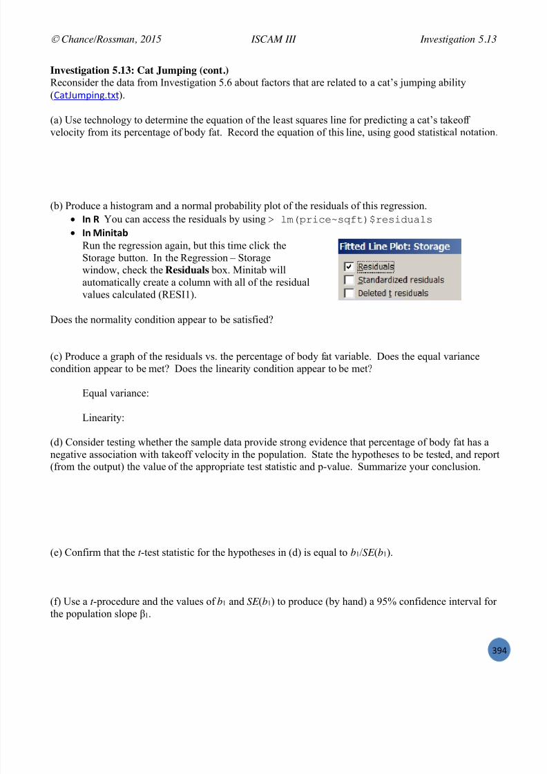
7/25/2019 Text: Investigating Statistical Concepts, Applications, and Methods
http://slidepdf.com/reader/full/text-investigating-statistical-concepts-applications-and-methods 395/428
Chance/Rossman, 2015 ISCAM III Investigation 5.13
#VP
Investigation 5.13: Cat Jumping (cont.)Reconsider the data from Investigation 5. 6 about factors that are related to a cat’s jumping ability(N&%c2*8'.3/%B%).
(a) Use technology to determine the equation of the least squares line for predicting a cat’s takeof f
velocity from its percentage of body fat. Record the equation of this line, using good statistical notation.
(b) Produce a histogram and a normal probability plot of the residuals of this regression. M* @You can access the residuals by using . 40&83?I;p9\G7*W3;9?A2B49 M* B8*8+"#
Run the regression again, but this time click theStorage button. In the Regression – Storage
window, check the Residuals box. Minitab willautomatically create a column with all of the residualvalues calculated (RESI1).
Does the normality condition appear to be satisfied?
(c) Produce a graph of the residuals vs. the percentage of body fat variable. Does the equal variancecondition appear to be met? Does the linearity condition appear to be met?
Equal variance:
Linearity:
(d) Consider testing whether the sample data provide strong evidence that percentage of body fat has anegative association with takeoff velocity in the population. State the hypotheses to be tested, and report(from the output) the value of the appropriate test statistic and p-value. Summarize your conclusion.
(e) Confirm that the t -test statistic for the hypotheses in (d) is equal to b1/SE (b1).
(f) Use a t -procedure and the values of b1 and SE (b1) to produce (by hand) a 95% confidence interval forthe population slope β 1.
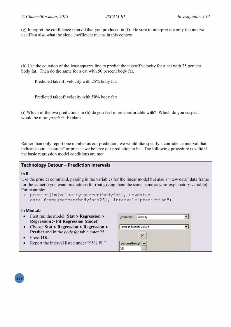
7/25/2019 Text: Investigating Statistical Concepts, Applications, and Methods
http://slidepdf.com/reader/full/text-investigating-statistical-concepts-applications-and-methods 396/428
Chance/Rossman, 2015 ISCAM III Investigation 5.13
#VR
(g) Interpret the confidence interval that you produced in (f). Be sure to interpret not only the intervalitself but also what the slope coefficient means in this context.
(h) Use the equation of the least squares line to predict the takeoff velocity for a cat with 25 percent body fat. Then do the same for a cat with 50 percent body fat.
Predicted takeoff velocity with 25% body fat:
Predicted takeoff velocity with 50% body fat:
(i) Which of the two predictions in (h) do you feel more comfortable with? Which do you suspectwould be more precise ? Explain.
Rather than only report one number as our prediction, we would like specify a confidence interval thatindicates our “accurate” or precise we believe our prediction to be. The following procedure is valid ifthe basic regression model conditions are met.
!%7=*'$'>6 2%+'4: – 9:%587+8'* M*+%:F"$,
M* @Use the 85,;')% command, passing in the variables for the linear model but also a “new data” data framefor the value(s) you want predictions for (but giving them the same name as your explanatory variable).For example:. 83;A?I7&40&H;4CI?71p8;3I;<7LCA1GB7*Q <;>AB7B!
AB7B=G3B0;&8;3I;<7LCA1GB7!#_*Q ?<7;3HB4!583;A?I7?C<5*
M* B8*8+"# First run the model ( Stat > Regression >
Regression > Fit Regression Model ).
ChooseStat > Regression > Regression >
Predict and in the body fat table enter 25. Press OK . Report the interval listed under “95% PI.”
7/25/2019 Text: Investigating Statistical Concepts, Applications, and Methods
http://slidepdf.com/reader/full/text-investigating-statistical-concepts-applications-and-methods 397/428
Chance/Rossman, 2015 ISCAM III Investigation 5.13
#VS
(j) Report the 95% prediction interval for the takeoff velocity of a cat with 25% body fat fromR/Minitab. Also determine the midpoint of this interval; does its value look familiar? Also interpretwhat this interval reveals.
Prediction interval:
Midpoint:
Interpretation:
(k) Repeat (j) to obtain a 95% prediction interval for the takeoff velocity of a cat with 50% body fat.Which interval is wider? Is this what you predicted in (i)?
As you saw in Investigation 2.6, the level of precision will also depend on whether we want to predictthe mean response or an individual response outcome.
Definition: Statistical packages compute both “prediction intervals” and “confidence intervals.” A prediction interval gives us the interval of plausible values for an individual response at a particularvalue of the explanatory variable. A confidence interval gives us the set of plausible values for themean response at a particular value of the explanatory variable.
!%7=*'$'>6 2%+'4: )'*(85%*7% M*+%:F"$,M* @I use ?<7;3HB4!5IC<G?A;<I;5 M* B8*8+"#I Now report the 95% CI output.
(l) What does R/Minitab report for the 95% confidence interval for the average takeoff velocity amongall cats that have 25% body fat? Also determine the midpoint of this interval; does its value lookfamiliar? Also interpret what this interval reveals.
Confidence interval:
Midpoint:
Interpretation:
(m) How does the interval in (l) compare to the interval in (j)? Why does this relationship make sense?Explain.

7/25/2019 Text: Investigating Statistical Concepts, Applications, and Methods
http://slidepdf.com/reader/full/text-investigating-statistical-concepts-applications-and-methods 398/428
Chance/Rossman, 2015 ISCAM III Investigation 5.13
#VT
0+456 )'*7$4,8'*,Technology tells us that we are 95% confident that a cat with 25% body fat would have a takeoffvelocity between 292.4 and 405.3 cm/sec. But if we were to consider the population of all cats with25% body fat, we are 95% confident that the mean takeoff velocity of these cats is between 335.5 and362.2 cm/sec, a much narrower interval. These procedures are valid because the analysis of the residual
plots did not reveal any strong departures from the basic regression model conditions.
Note: As with other t procedures, these procedures are fairly robust to the normality condition if youhave a larger sample size except the prediction interval calculation.
9:"7+87% 9:'#$%; VDHT Reconsider the 5K race results (I&--,6Ru!XW#/%B%) from Investigation 5.10.(a) Determine and interpret a 95% confidence interval for the mean finishing time of all 25-year-oldrunners in the population.(b) Joy Montoya, a 43-year-old female, did not appear in the first set of results. Use these data to predicther finishing time.(c) How do the intervals in (a) and (b) compare – Midpoint? Width? Explain why each has changed (ornot) the way it has.(d) Repeat (b) and (c) for Laure James, a 53-year-old female who also didn’t appear in the originalresults.(e) Do you consider the above interval calculations to be valid? (Examine and discuss residual plots.)
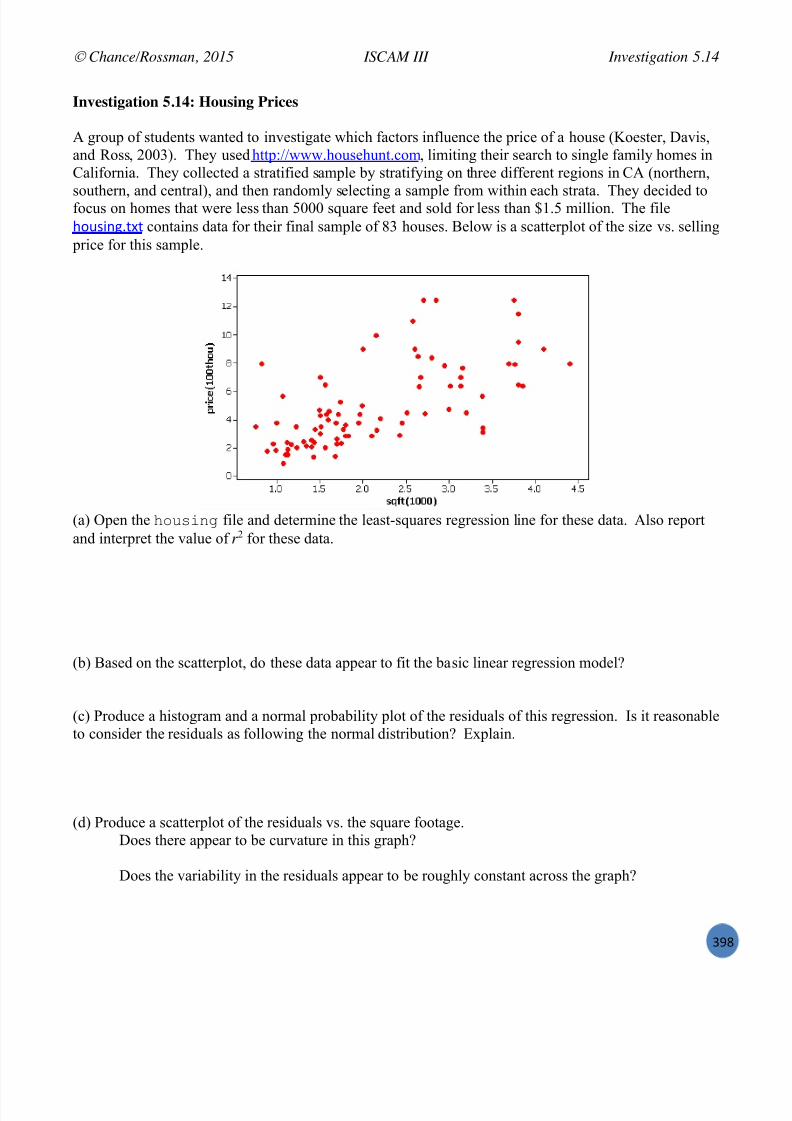
7/25/2019 Text: Investigating Statistical Concepts, Applications, and Methods
http://slidepdf.com/reader/full/text-investigating-statistical-concepts-applications-and-methods 399/428
Chance/Rossman, 2015 ISCAM III Investigation 5.14
#VU
Investigation 5.14: Housing Prices
A group of students wanted to investigate which factors influence the price of a house (Koester, Davis,and Ross, 2003). They used http://www.househunt.com , limiting their search to single family homes inCalifornia. They collected a stratified sample by stratifying on three different regions in CA (northern,
southern, and central), and then randomly selecting a sample from within each strata. They decided tofocus on homes that were less than 5000 square feet and sold for less than $1.5 million. The file+12('.3/%B% contains data for their final sample of 83 houses. Below is a scatterplot of the size vs. selling
price for this sample.
(a) Open the 6C29?<D file and determine the least-squares regression line for these data. Also reportand interpret the value of r 2 for these data.
(b) Based on the scatterplot, do these data appear to fit the basic linear regression model?
(c) Produce a histogram and a normal probability plot of the residuals of this regression. Is it reasonableto consider the residuals as following the normal distribution? Explain.
(d) Produce a scatterplot of the residuals vs. the square footage.Does there appear to be curvature in this graph?
Does the variability in the residuals appear to be roughly constant across the graph?

7/25/2019 Text: Investigating Statistical Concepts, Applications, and Methods
http://slidepdf.com/reader/full/text-investigating-statistical-concepts-applications-and-methods 400/428
Chance/Rossman, 2015 ISCAM III Investigation 5.14
#VV
Discussion : It takes a while to become comfortable interpreting these residual plots, but the housingdata do appear to have some problems. The residuals appear to cluster closer to zero for the smallerhouses and to have more variability for the larger houses. This violates the condition of a constantstandard deviation for each value of x. There is also a very slight hint of some curvature in this graph.The distribution of the residuals is clearly non-normal. This residual analysis gives us several reasons to
not apply the basic regression model to these data.
When the regression model conditions are violated, we can often transform the data in the hopes that thenew variables do meet the conditions.
(e) Take the log base 10 of both the house prices and sizes, storing the results as logprice and logsqft .[ Hint : In Minitab, use Calc > Calculator or the 4;7 command. Also keep in mind that both R andMinitab assume natural log when use the “log” function. In Minitab use “logten” and in R use “log10”.] Produce the scatterplot and determine the regression equation to model the relationship between thesetwo variables, storing the residuals. Examine the residual plots (histogram of residuals and residualsversus explanatory variable). Do these transformed variables appear to be more suitable for the basic
regression model? Explain.
(f) Interpret the slope coefficient in the regression model using the log transformed variables.
(g) Use the least squares regression line to predict the cost of a 3,000 square foot house. [ Hints :Substitute log 10(3000) into the right hand side of the equation to obtain a prediction for the log 10(price) ,and then raise 10 to this power to determine the predicted price. Similarly, you can back transform theendpoints of the confidence and prediction intervals from R/Minitab.]
Discussion: The log transformation has made improvements for both the normality condition and theequal variance condition. It is not uncommon for one transformati on to “correct” more than one
problem. We could continue to explore other transformations (e.g., square root and powertransformations) until we find transformed data that are more appropriate for the basic regression model.Although these transformations are useful, we then have to be careful in how we interpret the regressioncoefficients and make predictions. If possible, it is usually most useful to “back -transform” to theoriginal scale.

7/25/2019 Text: Investigating Statistical Concepts, Applications, and Methods
http://slidepdf.com/reader/full/text-investigating-statistical-concepts-applications-and-methods 401/428
Chance/Rossman, 2015 ISCAM III Investigation 5.14
PXX
9:"7+87% 9:'#$%; VDHU The datafile <&-*&5%/%B% contains data on the number of stores and the number of SuperCenters thatWal-Mart had in operation between 1989 and 2002.(a) Create a scatterplot of the number of SuperCenters that Wal-Mart has had in operation versus time.(b) Would it be appropriate to use the basic regression model for these data? Explain.
(c) Transform the SuperCenters variable by taking the square root. Would it be appropriate to use the basic regression model for the relationship between this variable and year? Explain.(d) Transform the SuperCenters variable by taking the natural log. Would it be appropriate to use the
basic regression model for the relationship between this variable and year? Explain.(e) Choose the best model from either (c) or (d) (and justify your choice), find the least-squaresregression equation and use it to predict how many SuperCenters Wal-Mart had in operation in 2003.(f) Report and interpret a 95% prediction interval for 2003.
04;;":6 '( M*(%:%*7% (': @%>:%,,8'*
To test H 0: 1 = hypothesized slope vs. H a: 1 ≠ hypothesized slope
The test statistic: t =)( 1
1bSE
sloped hypothsizeb follows a t-distribution with df = n 2
An approximate 100 ! C% confidence interval formula is b1 + t n 2 SE(b1) where t n 2 is the100 ! (1 C)/2 percentile of the student t-distribution with n 2 degrees of freedom.
These procedures are valid as long as L: There is a linear relationship between the response and explanatory variable.
I: The observations are independent. N: The response follows a normal distribution for each value of x. E: The standard deviation of the responses is the equal at each value of x.
These conditions are checked by examining the residual plots: residuals vs. explanatory variable andhistogram/normal probability plot of the residuals.
The Analyzing Two Quantitative Variables applet, Minitab ( Stat > Regression > Regression > FitRegression Model ), and R ( .9200B31&40&3;98C<9;p;[84B<B7C31* all automatically reportthe two-sided p-value. This p-value can be divided in half to obtain a one-sided p-value (assuming theobserved slope is in the direction conjectured).
Discussion : Typically we are most interested in testing whether the population slope coefficient equalszero, as that would suggest that the population regression line is flat and so the explanatory variable is ofno use in predicting the response variable. Because testing whether the slope coefficient is zero testswhether the regression model with this explanatory variable is of any use, it is sometimes called a modelutility test .

7/25/2019 Text: Investigating Statistical Concepts, Applications, and Methods
http://slidepdf.com/reader/full/text-investigating-statistical-concepts-applications-and-methods 402/428
Chance/Rossman, 2015 ISCAM III Exploration
PXW
There are situations where we might want to test other values of the population slope, for example 1 =1 (do x and y change at the same rate?). We can also use the same approach to carry out tests andcreate confidence intervals for the population intercept. However, these are less useful in practice, inparticular because the intercept is often far outside the range of data and does not have a meaningfulinterpretation.
Checking the technical conditions is an important step of the process. Notice that you will typically fitthe regression model first to obtain the residuals to allow you to assess the model. As with ANOVA,these t procedures are fairly robust to departures from normality. If the conditions are violated, you canagain explore transformations of the data.
!%7=*'$'>6 /A?$':"+8'*I !=% @%>:%,,8'* /((%7+
In the 2013 Masters golf tournament, Spaniard Sergio Garcia had a score of 66 in the first round but ascore of 76 in the second round. Keep in mind that in golf, lower scores are better than higher scores. Isthis evidence that he choked? The data file C&(%,5(W#/%B% contains golfers’ scores in the first two roundsof the 2013 Masters.
(a) Use technology to construct a scatterplot of second round score vs. first round score. Also calculatethe correlation between these two. Does it reveal an association between scores in these two rounds? Ifso, is it positive or negative? Would you call it weak, moderate, or strong?
(b) Use technology to sort the data according to the golfers’ first -round scores: M* @
. 01AB7B!AB7B=G3B0;&DC4G;3Q 3C2<A,Q 3C2<A#*
. 9C37AB7B!01AB7BiC3A;3&01AB7BiQ#k*Qk M* B8*8+"#
NUe. 9C37 I,)I( I_)IcOKJe". L1 I#=Or Choose Data > Sort , entering movie, score, and rating in the Sort columns box and score inthe By column box.
List the ten golfers who scored lowest in the first round, along with their scores in both rounds. Thenlist the ten golfers who scored highest in the first round, along with their scores in both rounds.
(c) How many of the “top ten” from the first round improved (scored lower) in the second round thanthe first? How many of the “bottom ten” from the first round improved?
(d) Which group saw more people improve? Is this difference small or substantial?

7/25/2019 Text: Investigating Statistical Concepts, Applications, and Methods
http://slidepdf.com/reader/full/text-investigating-statistical-concepts-applications-and-methods 403/428
Chance/Rossman, 2015 ISCAM III Exploration
PX!
(e) Determine the median second round score for the two groups (the “top ten” from round one and the“bottom ten” from round one). Which group tended to score better (lower) in the second round?
(f) Add the “ y = x” line t o your scatterplot. M* @I .4?<;9&3C2<A,Q 3C2<A,* M* B8*8+"#I Right click on your scatterplot and choose Add > Calculated Line . Enter the sorted
scores as the Y column and as the X column.Identify any golfers by name who improved in the second round after scoring in the top ten of the firstround. Identify any golfers by name who did worse in the second round after scoring in the bottom tenof the first round.
(g) Do you think the “ y = x” line does a good job of summarizing the relationship? How do you think the regression line will compare? Will the slope be greater or smaller?
(h) Add the y line to the scatterplot. M* @I . BL4?<;&6!0;B<&3C2<A,** M* B8*8+"#I Right click on your scatterplot and choose Add > Reference Lines . Enter 74.196 in
the “Show reference lines at Y values ” box and click OK .Do you think this line does a good job of summarizing the relationship? How do you think theregression line will compare? Will the slope be greater or smaller?
(i) Now add the regression line to the scatterplot. M* @I . BL4?<;&40&3C2<A,p3C2<A#*Q IC4!(* M* B8*8+"#I Right click on the scatterplot and choose Add > Regression Fit .
Where does the regression line fall compared to the two earlier lines?
(j) Determine the regression equation. Is the slope less than one? Explain why this is to be expectedwhenever the two standard deviations are similar.[ Hint : Recall that the slope coefficient can be expressed as b = r(s y)/(s x).]
7/25/2019 Text: Investigating Statistical Concepts, Applications, and Methods
http://slidepdf.com/reader/full/text-investigating-statistical-concepts-applications-and-methods 404/428
Chance/Rossman, 2015 ISCAM III Exploration
PX#
(k) Explain why your answer to (j) suggests that golfers with poor first round scores will tend to improve but golfers with good first round scores will tend to worsen.
This phenomenon is sometimes called the regression effect or regression to the mean. Sir FrancisGalton first discussed this effect in the late 1880s when he examined data on the heights of parents andchildren, calling it regression to mediocrity. 0%7+8'* VDU 04;;":6
You continued to study least squares regression in this section, turning to issues of inference . Youlearned the conditions of the basic regression model (linearity, independence, normality, and equalvariance), and once again you used simulation to study the approximate sampling distribution assumingthe null hypothesis is true, this time for sample regression coefficients. You found that the t-distributioncan be used to perform significance tests and construct confidence intervals for regression coefficient
parameters and for predicted values, based on sample data. The primary significance test of interest isusually whether the sample data provide evidence of an association in the population between the twovariables, which is equivalent to testing whether the population slope coefficient equals zero. You alsolearned how to use residual plots to check the technical conditions associated with the basic regressionmodel. Example 5.3 illustrates an application of regression analysis.

7/25/2019 Text: Investigating Statistical Concepts, Applications, and Methods
http://slidepdf.com/reader/full/text-investigating-statistical-concepts-applications-and-methods 405/428
Chance/Rossman, 2015 ISCAM III Example 5.1
PXP
Example 5.1: Internet Use by RegionTry these questions yourself before you use the solutions following to check your answers.
The Pew Internet and American Life Project examines how Americans use the internet. In 2002 theorganization took random samples of people from across the country and asked questions about their use
of the internet. Consider the following information from this study:Northeast South Midwest WestSample size 3973 4332 4929 5137
# of internet users 2417 2372 2831 3259Analyze these data to address the question of whether internet use varies across these four regions of thecountry. Include graphical and numerical summaries as well as a test of significance. Summarize yourconclusions.

7/25/2019 Text: Investigating Statistical Concepts, Applications, and Methods
http://slidepdf.com/reader/full/text-investigating-statistical-concepts-applications-and-methods 406/428
Chance/Rossman, 2015 ISCAM III Example 5.1
PXR
<*"$6,8,We will treat the samples taken by the Pew organization as independent random samples from these fourregions of the country. With a binary response variable (internet user or not) and more than two groupsto compare, we will use a chi-square analysis.
Let i represent the actual population proportion of internet users in region i. Then the hypotheses to betested are:
H0: NE = S = MW = W
(The population proportions of internet users are the same for all four regions.)Ha: The population proportion of internet users is different in at least one region.
The two-way table of observed counts is:Northeast South Midwest West Total
Internet users 2417 2372 2831 3259 10,879Non-internet users 1556 1960 2098 1878 7492Total 3973 4332 4929 5137 18,371
The sample proportions of internet users in the four regions are:Northeast South Midwest West Total
Proportion of internet users .608 .548 .574 .634 .592
A segmented bar graph to display these data is:
We notice that the proportions of internet users do not vary too much across these four regions. Thewest has the highest proportion, with about 63% internet use, and the south has the smallest with only55% internet use.
To see whether at least one of these regions is statistically significant different from the others, we usetechnology to determine the expected counts, chi-square test statistic, and p-value. Below is Minitaboutput:
0%
20%
40%
60%
80%
100%
N o r t h e
a s t
S o u t h
M i d w
e s t
W e s t
region
Non-internet users
Internet users

7/25/2019 Text: Investigating Statistical Concepts, Applications, and Methods
http://slidepdf.com/reader/full/text-investigating-statistical-concepts-applications-and-methods 407/428
Chance/Rossman, 2015 ISCAM III Example 5.1
PXS
'[8;I7;A IC2<79 B3; 83?<7;A L;4C> CL9;3H;A IC2<79"6?)K\2B3; IC<73?L27?C<9 B3; 83?<7;A L;4C> ;[8;I7;A IC2<79
gC376;B97 KC276 N?A>;97 u;97 UC7B4, #],c #(c# #a(, (#_b ,-acb
#(_#=c] #_^_=(] #b,a=ac (-]#=-_,=c__ ,]=_c, #=^]_ ,_=]c(
# ,__^ ,b^- #-ba ,aca c]b#,^#-=#^ ,c^^=^^ #-,-=,( #-b]=b_
#=_]a #,=,_a (=a], ##=]^a
UC7B4 (bc( ]((# ]b#b _,(c ,a(c,
"6?)K\ ! a]=]^-Q %R ! (Q f)VB42; ! -=---
This procedure is valid because all of the expected counts are far larger than 5, and we areassuming that the Pew organization took independent random samples across the regions. Their reportmentions that they used random digit dialing with extensive follow- up efforts, but it’s not clear whetherthey took independent samples within these regions or took a nationwide sample and treated region asone of the variables. Either way the chi-square analysis is valid.
The p-value is extremely small (0.000 to three decimal places), indicating that the differencesobserved in the sample proportions would almost never occur by chance if the population proportionswere really equal across the four regions. Thus, we have overwhelming evidence to reject the nullhypothesis and conclude that the proportions of internet users are not the same in these four regions.
In an effort to say a little bit more, we can examine the cell contributions. We see that the largestcontributions occur in the West and South. The West had more internet users, 3259, (and so fewer non-internet users) than would have been expected if the proportions were all the same, 3042.05, and theSouth had fewer internet users, 2372, (and so more non-users) than would have been expected, 1766.66.The observed counts in the Northeast and Midwest regions were fairly close to the expected counts.
In conclusion, the sample data provide very strong evidence that the population proportions ofinternet users differ across regions of the United States. The differences in the sample proportions arelarger than can reasonably be explained by random sampling variation. The large sample sizes in thisstudy help to render the differences among the samples statistically significant even though the sample
proportions seem to be fairly similar in practical terms.

7/25/2019 Text: Investigating Statistical Concepts, Applications, and Methods
http://slidepdf.com/reader/full/text-investigating-statistical-concepts-applications-and-methods 408/428
Chance/Rossman, 2015 ISCAM III Example 5.2
PXT
Example 5.2: Lifetimes of Notables
The 1991 World Almanac and Book of Facts contained a section on “noted personalities” in a total ofnine occupational categories. The lifetimes of these people can be found in the -'9,%'*,(Q2--/%B% data file.Analyze these data to address the question of whether the average lifetimes across these occupational
categories differ significantly. Include graphical and numerical summaries as well as a test ofsignificance. Summarize your conclusions.
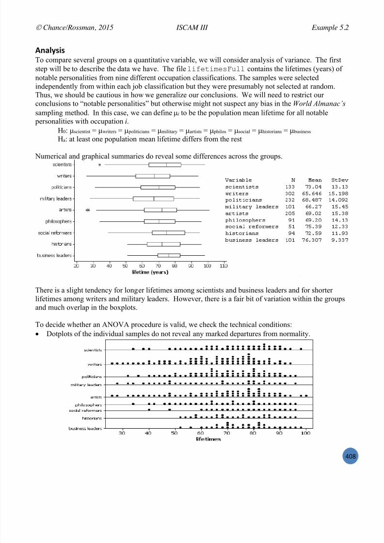
7/25/2019 Text: Investigating Statistical Concepts, Applications, and Methods
http://slidepdf.com/reader/full/text-investigating-statistical-concepts-applications-and-methods 409/428
Chance/Rossman, 2015 ISCAM III Example 5.2
PXU
<*"$6,8,To compare several groups on a quantitative variable, we will consider analysis of variance. The firststep will be to describe the data we have. The file 4?G;7?0;9R244 contains the lifetimes (years) ofnotable personalities from nine different occupation classifications. The samples were selectedindependently from within each job classification but they were presumably not selected at random.
Thus, we should be cautious in how we generalize our conclusions. We will need to restrict ourconclusions to “notable personalities” but otherwise might not suspect any bias in the World Almanac’s sampling method. In this case, we can define i to be the population mean lifetime for all notable
personalities with occupation i.H0: scientist = writers = politicians = military = artists = philos = social = historians = business Ha: at least one population mean lifetime differs from the rest
Numerical and graphical summaries do reveal some differences across the groups.
There is a slight tendency for longer lifetimes among scientists and business leaders and for shorterlifetimes among writers and military leaders. However, there is a fair bit of variation within the groupsand much overlap in the boxplots.
To decide whether an ANOVA procedure is valid, we check the technical conditions: Dotplots of the individual samples do not reveal any marked departures from normality.

7/25/2019 Text: Investigating Statistical Concepts, Applications, and Methods
http://slidepdf.com/reader/full/text-investigating-statistical-concepts-applications-and-methods 410/428
Chance/Rossman, 2015 ISCAM III Example 5.2
PXV
The ratio of the largest to smallest standard deviations (15.45/9.34) is less than 2 so we will assumethat the population variances are equal.
We have independent samples from each population though the randomness condition isquestionable.
Although we do not have randomness in this study, we will still explore whether the difference betweenthe sample means is larger than we would expect by chance.
The large test statistic F = 9.36 and small p-value (0.000 < 0.001) provide strong evidence that the population mean lifetime for at least one of these occupations differs from the rest.
Because this was an observational study, we cannot draw any cause and effect conclusions and asdiscussed above we should be cautious in generalizing these conclusions beyond the 1310 individuals inthe study as they were not randomly selected. For the individuals in this study, there appears to besomething other than random chance to account for the differences we observed in their lifetimes.

7/25/2019 Text: Investigating Statistical Concepts, Applications, and Methods
http://slidepdf.com/reader/full/text-investigating-statistical-concepts-applications-and-methods 411/428
Chance/Rossman, 2015 ISCAM III Example 5.3
PWX
Example 5.3: Physical Education Class Performance
A physical education teacher at a junior high school in Central California wanted to determine whetherthere is a relationship between seventh- graders’ times to run a mile and how many push -ups they can dounder controlled conditions. She collected the data in OfN-&((/%B% as part of the mandated state physical
fitness testing program. Analyze these data to address the question of whether they provide evidence ofa relationship between these two variables. Include graphical and numerical summaries as well as a testof significance. Summarize your conclusions.

7/25/2019 Text: Investigating Statistical Concepts, Applications, and Methods
http://slidepdf.com/reader/full/text-investigating-statistical-concepts-applications-and-methods 412/428
Chance/Rossman, 2015 ISCAM III Example 5.3
PWW
<*"$6,8,Because we have two quantitative variables here (time to run one mile and number of push-ups), theappropriate analysis would be regression. We first want to examine numerical and graphical summaries.When you open f'"4B99 you will notice that the mile run times have been recorded in “time format.”We want to convert this to numerical values. For example, in Minitab choose Data > Change Data Type
> Data/Time to Numeric. Specify C3 as the column to be changed and C4 as the storage location for theconverted values. The data are now numeric, but in terms of a 24-hour day. To convert these back tominutes, type
NUe. 4;7 I_!I]+#] or use Calc > Calculator, letting miletime = 24*c4. Now you should have the number of minutes (including the fraction of minute) for each student.
Because we aren’t considering either of these as a response v ariable, it does not matter which variablewe denote as the y-variable and which as the x-variable. If we plot mile time vs. push-ups, we see thereis a strong negative association.
Students who do more push-ups also tend to run the mile in faster times. However, there is someevidence that the relationship is not linear. There is also an unusual observation, a student who did alarger number of push-ups but was one of the slowest runners. Carrying out the regression andexamining residual plots confirms these observations.

7/25/2019 Text: Investigating Statistical Concepts, Applications, and Methods
http://slidepdf.com/reader/full/text-investigating-statistical-concepts-applications-and-methods 413/428
Chance/Rossman, 2015 ISCAM III Example 5.3
PW!
The residual vs. explanatory variable graph also reveals some differences in the amount of variation inthe residuals at different values of the explanatory variable (indicating a violation of the constantvariance condition).
It appears that transforming these data might be helpful. Because both distributions appear skewed to
the right (if you looked at histograms of each variable individually), we could considering taking the logof each variable. The log-log scatterplot does appear more well behaved. (We have used log base ten but natural logs would also work.)
We still have some outliers but appear to now have a linear relationship. If we also examine thenormality of the residuals:
This condition also seems to be reasonably met for the transformed data. There is slight evidence ofskewness to the right in the residuals but coupled with the large sample size we will not be concernedwith this minor deviation.
The correlation coefficient for the transformed variables is 0 .624, indicating a moderately strongnegative linear relationship between log(time) and log(push-ups). The least-squares regression equation
is computed by Minitab to be^
log mile = 1.23 0.213 log( push-ups ). The intercept coefficient here
would indicate the predicted log-time for a student who only completes 1 push up (so log( push-ups ) = 0)to be 1.23. This corresponds to a time of 10 1.23 or about 17 minutes. The slope coefficient predicts theaverage multiplicative change in the log-mile times for each unit increase in log( push-ups ). A unitincrease in “log( push-ups )” corresponds to the push -ups increasing by a factor of 10. So for each 10fold increase in the number of push-ups (e.g., 1 push up to 10 push-ups), the mile time decreases onaverage by a factor of 10 .213 = 0.61. [Note: our prediction for 10 push-ups is 1.017, corresponding to101.107 10.4 minutes, which is 0.61(17).]

7/25/2019 Text: Investigating Statistical Concepts, Applications, and Methods
http://slidepdf.com/reader/full/text-investigating-statistical-concepts-applications-and-methods 414/428
Chance/Rossman, 2015 ISCAM III Example 5.3
PW#
If we test the significance of this correlation:Let represent the true population slope between log(time) and log(push-ups)H0: = 0 (there is not association between these two variables)Ha: ≠ 0 (there is an association)
We find a test statistic of t = -10.48 and a two-sided p-value of approximately 0.
Note: This p-value is the same as reported by Minitab with the sample correlation coefficient.
With such a small p-value (< 0.001) we would consider the relationship between log(time) and log(push-ups) to be statistically significant. Although we need to have some caution in generalizing these resultsto other schools, we can eliminate “random chance” as an explanation for the strong log -log relationshipobserved in this sample.
If we wanted to use this model to carry out predictions, we need to keep the transformed nature of thevariables in mind. For example, if a student completed 25 push-ups during that portion of the test, wewould predict 1.23 0.213 log 10(25) = 0.932 for the log-time and therefore 10 .932 = 8.56 minutes for themile time. We also need to start being a little cautious in predicting the mile time for such a largenumber of push-ups as we do not have a large amount of data in this region and our estimate will not beas precise.
In summary, there is a strong negative relationship between number of push-ups and time to run a milefor this 7 th and 8 th graders as we would expect (those students who do more than the average number of
push-ups will tend to be the same students who complete a mile faster, in a below average time). Thisrelationship can be considered statistically significant after performing log transformations, however, wehave to be cautious in generalizing these results beyond this sample as the students were not randomlyselected from a larger population of junior high students. Because this is an observational study, we arenot claiming that doing more push-ups will cause the mile time to decrease.We also saw in an earlier example that there was a statistically significant difference between males andfemales on these tasks and we might want to consider incorporating that variable into our analysis aswell. For example, a coded scatterplot shows that the males tended to do more push-ups and also tendedto be slightly faster than females on the mile times.

7/25/2019 Text: Investigating Statistical Concepts, Applications, and Methods
http://slidepdf.com/reader/full/text-investigating-statistical-concepts-applications-and-methods 415/428
Chance/Rossman, 2015 ISCAM III Example 5.3
PWP
We can actually carry out a multiple regression analysis to predict mile time from both push ups and
gender .
This analysis reveals that push-ups are strongly related to mile times even after adjusting for gender(meaning this association is strong among the females and also among the males), but if you know thesomeone’s push -up count, it is not that valuable to also know their gender.

7/25/2019 Text: Investigating Statistical Concepts, Applications, and Methods
http://slidepdf.com/reader/full/text-investigating-statistical-concepts-applications-and-methods 416/428
Chance/Rossman, 2015 ISCAM III Example 5.4
PWR
Example 5.4: Comparing Popular Diets
Dansinger, Griffith, Gleason et al. (2005) report on a randomized, comparative experiment in which 160subjects were randomly assigned to one of four popular diet plans: Atkins, Ornish, Weight Watchers,and Zone (40 subjects per diet). These subjects were recruited through newspaper and television
advertisements in the greater Boston area; all were overweight or obese with body mass index values between 27 and 42. Among the variables measured were Which diet the subject was assigned to Whether or not the subject completed the twelve-month study The subject’s weight loss after two months, six months, and twelve months (in kilogra ms, with a
negative value indicating weight gain) The degree to which the subject adhered to the assigned diet, taken as the average of 12 monthly
ratings, each on a 1-10 scale (with 1 indicating complete non-adherence and 10 indicating fulladherence)
Data for the 93 subjects who completed the 12-month study are in the file N1*8&5'.3E',%(/ %B%.
Some of the questions that the researchers studied are:(a) Do the average weight losses after 12 months differ significantly across the four diet plans?(b) Is there a significant difference in the completion/dropout rates across the four diet plans?(c) Is there a significant positive association between a subject’s adherence level and his/ her amount ofweight loss?(d) Is there strong evidence that dieters actually tend to lose weight on one of these popular diet plans?
For each of these research questions, first identify the explanatory variable and the response variable,and classify each as categorical or quantitative. Then use graphical and numerical summaries toinvestigate the question, and summarize your findings. Next, identify the inference technique that can
be used to address the question, and apply that technique. Be sure to include all aspects of the
procedure, including a check of its technical conditions. Finally, summarize your conclusions for eachquestion. Write a paragraph summarizing your findings from these four analyses. [ Hint : To determinethe completion rate for each diet, count how many of the 93 subjects who completed the study are ineach diet group and compare those counts to the 40 that were originally assigned to each diet.]

7/25/2019 Text: Investigating Statistical Concepts, Applications, and Methods
http://slidepdf.com/reader/full/text-investigating-statistical-concepts-applications-and-methods 417/428
Chance/Rossman, 2015 ISCAM III Example 5.4
PWS
<*"$6,8,(a) Effect of diet plan on average weight loss: The explanatory variable is diet plan, which is categorical.The response variable is amount of weight loss after 12 months, which is quantitative. Boxplots andnumerical summaries follow:
A?;7 g N;B< K7%;H N;A?B< YtPS7@?<9 #, (=b# ^=-_ (=b- b=,_ (all in kilograms) h3<?96 #- ^=_^ b=#b _=]_ ^=a, (all in kilograms) uD7 uB7I6 #^ ]=_b _=(b (=^- ^=a_ (all in kilograms) vC<; #^ ]=aa ^=b# (=]- a=^( (all in kilograms)
These boxplots and statistics seem to indicate that the four diets do not differ substantially with regard toweight loss after 12 months. The mean and median weight loss are both positive for all four diets,indicating that subjects did tend to lose some weight on these diets, roughly 4-6 kilograms on average.The boxplots also show substantial overlap between the four distributions. The means and medians arevery similar for three of the diets, with the Ornish diet having a somewhat larger mean and medianweight loss (6.56 and 5.45 kilograms, respectively) than the others. All four distributions of weight lossappear to be fairly symmetric, perhaps a bit skewed to the right. The variability in weight losses is alsosimilar across all four diet plans, with the Ornish diet having the most variability, largely due to its onesmall and three large outliers.
Because we have a categorical explanatory variable and a quantitative response variable, we will apply
ANOVA to these data. The technical conditions appear to be met: The subjects were randomly assignedto diet plans, the distributions look fairly normal (see the following normal probability plots), and thestandard deviations are similar (ratio of largest to smallest is 9.29/5.39, which is less than 2).
! " # $
%#"&'$ )*++
!"#$
%$&'() %+),($-.
/-#&.(
0)1&#.
2343533653

7/25/2019 Text: Investigating Statistical Concepts, Applications, and Methods
http://slidepdf.com/reader/full/text-investigating-statistical-concepts-applications-and-methods 418/428
Chance/Rossman, 2015 ISCAM III Example 5.4
PWT
The hypotheses are:
H0: A = O = W = Z, where i represents the underlying treatment mean weight loss after 12 monthswith diet i. This hypothesis says that the treatment mean is the same for all four diets.
Ha: that at least two of the treatment means differ; in other words, that at least one diet does have adifferent treatment mean than the others
Minitab produces the following ANOVA table: KC23I; %R KK NK R fA?;7 ( cc=^ #_=b -=_] -=^_b'33C3 ab ]#b(=c ]a=#UC7B4 b# ](c,=(
The small F -statistic ( F = 0.54) and large p-value (0.659) reveals that the experimental data provideessentially no evidence against the null hypothesis. The p-value reveals that differences among thegroup means at least as big as those found in this experiment would occur about 66% of the time byrandomization alone even if there were no true differences among the diets. In other words, thetreatment means do not differ significantly, and there is no evidence that these four diets producedifferent average amounts of weight loss.
(b) Effect of diet plan on completion rate: The explanatory variable is diet plan, which is categorical.The response variable is whether the subject completed the study or dropped out, which is alsocategorical.
The two-way table of completion/dropout status by diet plan, followed by completion proportions and asegmented bar graph:
Atkins Ornish WeightWatchers
Zone
Completed 21 20 26 26Dropped out 19 20 14 14Completion proportion .525 .500 .650 .650
%#"&'$ )*++
, # - . # /
$
73433643
88
83
93
53
5
73433643
88
83
93
53
5
0)1&#. /-#&.(
%$&'() %+),($-. !"#$
,-*010")"$2 ,)*$ *3 %#"&'$ )*++:"-;+< 6 89= >?

7/25/2019 Text: Investigating Statistical Concepts, Applications, and Methods
http://slidepdf.com/reader/full/text-investigating-statistical-concepts-applications-and-methods 419/428
Chance/Rossman, 2015 ISCAM III Example 5.4
PWU
This preliminary analysis appears to reveal that the completion rates are very similar across the four diet
plans. Weight Watchers and Zone tied for the highest completion rate (62.5%), with Ornish having thelowest completion rate (50%), but these do not seem to differ substantially.
To test whether these differences in the distributions of the categorical response variable are statisticallysignificant, we can apply a chi-square test of the hypotheses:
H0: A = O = W = Z, where i represents the underlying completion rate after 12 months with diet i(diet does not have an effect on completion rate)
Ha: at least two of the underlying completion rates differ (there is a difference in underlyingcompletion rates across the 4 diets)
Minitab produces the following output:
u;?D67S7@?<9 h3<?96 uB7I6;39 vC<; UC7B4, #, #- #^ #^ b(
#(=#_ #(=#_ #(=#_ #(=#_-=#,a -=]_] -=(#_ -=(#_
# ,b #- ,] ,] ^c,^=c_ ,^=c_ ,^=c_ ,^=c_-=(-# -=^(, -=]_, -=]_,
UC7B4 ]- ]- ]- ]- ,^-
"6?)K\ ! (=,_aQ %R ! (Q f)VB42; ! -=(^a
Checking the technical conditions of the chi-square procedure, we note that the subjects were randomlyassigned to a diet plan group and that all expected counts in the table are larger than 5 (smallest is16.75), so we are justified in applying the chi-square test. The p-value of 0.368 says that if there were nodifference in the underlying completion rates (i.e., no treatment effect) of completion among the fourdiet plans, then it would not be surprising (probability 0.368) to obtain experimental completion
proportions that differ as much as these do. Because this p-value is not small, we can conclude only that
0%10%20%30%40%50%60%70%80%90%
100%
Atkins Ornish WeightWatchers
Zone
Dropped outCompleted

7/25/2019 Text: Investigating Statistical Concepts, Applications, and Methods
http://slidepdf.com/reader/full/text-investigating-statistical-concepts-applications-and-methods 420/428
Chance/Rossman, 2015 ISCAM III Example 5.4
PWV
the experimental data do not provide evidence to suggest that the completion proportions differ acrossthese four diet plans.
(c) Association between adherence and weight loss: The explanatory variable is adherence level. Thisvariable is quantitative. (It could be considered categorical if it were simply on a 1 10 scale, but it is the
average of 12 such values and so should be treated as quantitative.) The response variable is weightloss, which is quantitative.
A scatterplot of weight loss vs. adherence level follows:
This graph reveals a moderately strong, positive, linear relationship between weight loss and adherencelevel. The correlation coefficient can be found to be r = 0.518. The scatterplot and correlationcoefficient both suggest that there is a positive association between these variables, that subjects withhigher adherence levels tend to lose more weight.
We can fit a regression line for predicting weight loss from adherence level:
This model indicates that for each additional step on the adherence level scale, the subject is predicted tolose an additional 2.4 kilograms of weight.
1!'#-#/.# )#4#)
% #
" & ' $ ) * + +
538@AB97245
23
43
53
3
653
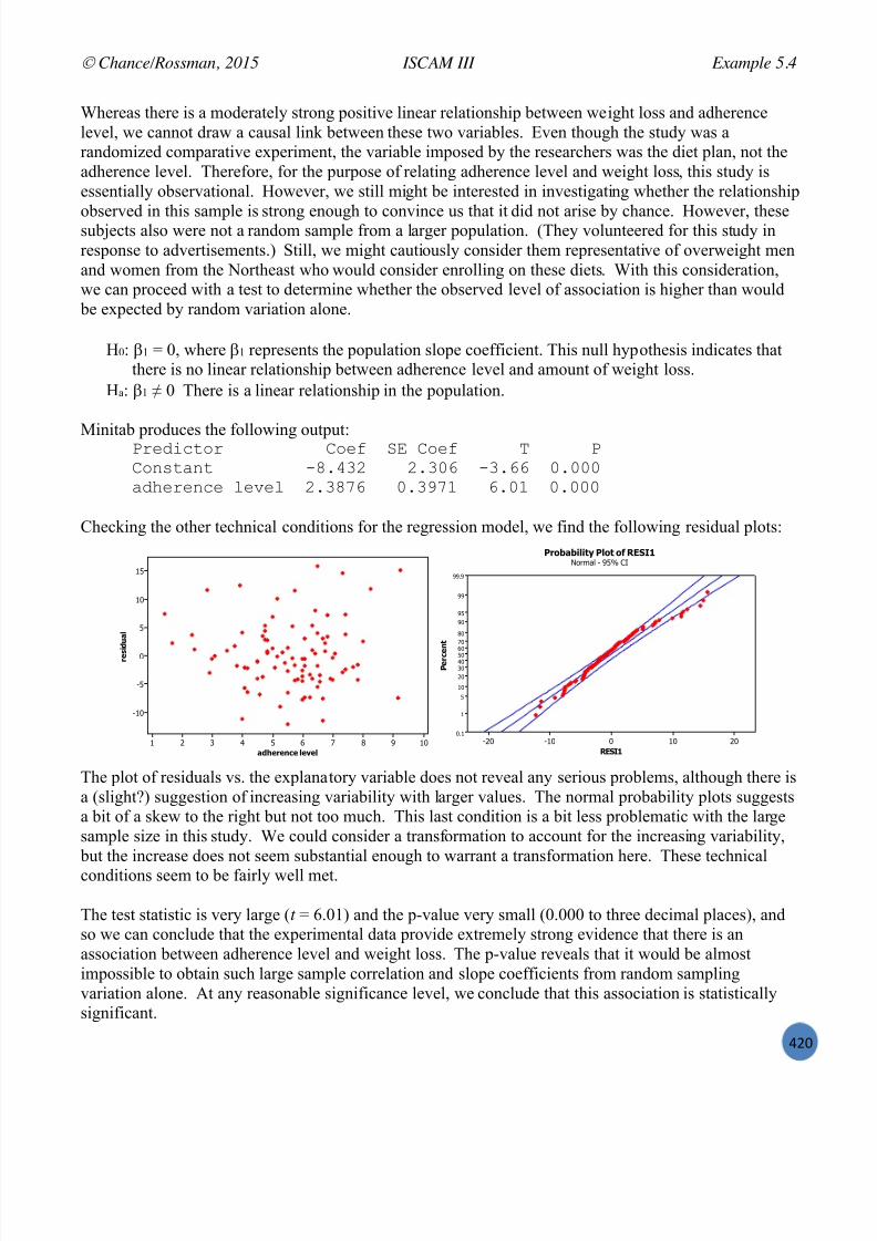
7/25/2019 Text: Investigating Statistical Concepts, Applications, and Methods
http://slidepdf.com/reader/full/text-investigating-statistical-concepts-applications-and-methods 421/428
Chance/Rossman, 2015 ISCAM III Example 5.4
P!X
Whereas there is a moderately strong positive linear relationship between weight loss and adherencelevel, we cannot draw a causal link between these two variables. Even though the study was arandomized comparative experiment, the variable imposed by the researchers was the diet plan, not theadherence level. Therefore, for the purpose of relating adherence level and weight loss, this study isessentially observational. However, we still might be interested in investigating whether the relationship
observed in this sample is strong enough to convince us that it did not arise by chance. However, thesesubjects also were not a random sample from a larger population. (They volunteered for this study inresponse to advertisements.) Still, we might cautiously consider them representative of overweight menand women from the Northeast who would consider enrolling on these diets. With this consideration,we can proceed with a test to determine whether the observed level of association is higher than would
be expected by random variation alone.
H0: 1 = 0, where 1 represents the population slope coefficient. This null hypothesis indicates thatthere is no linear relationship between adherence level and amount of weight loss.
Ha: 1 ≠ 0 There is a linear relationship in the population.
Minitab produces the following output:f3;A?I7C3 "C;G K' "C;G U f"C<97B<7 )a=](# #=(-^ )(=^^ -=---BA6;3;<I; 4;H;4 #=(ac^ -=(bc, ^=-, -=---
Checking the other technical conditions for the regression model, we find the following residual plots:
The plot of residuals vs. the explanatory variable does not reveal any serious problems, although there isa (slight?) suggestion of increasing variability with larger values. The normal probability plots suggestsa bit of a skew to the right but not too much. This last condition is a bit less problematic with the largesample size in this study. We could consider a transformation to account for the increasing variability,
but the increase does not seem substantial enough to warrant a transformation here. These technicalconditions seem to be fairly well met.
The test statistic is very large ( t = 6.01) and the p-value very small (0.000 to three decimal places), andso we can conclude that the experimental data provide extremely strong evidence that there is anassociation between adherence level and weight loss. The p-value reveals that it would be almostimpossible to obtain such large sample correlation and slope coefficients from random samplingvariation alone. At any reasonable significance level, we conclude that this association is statisticallysignificant.
1!'#-#/.# )#4#)
- # + " ! 5 1
)
538@AB97245
59
53
9
3
69
653
6789:
, # - . # /
$
43533653643
88C8
88
8983
@3A3B393732343
53
9
5
3C5
,-*010")"$2 ,)*$ *3 6789::"-;+< 6 89= >?
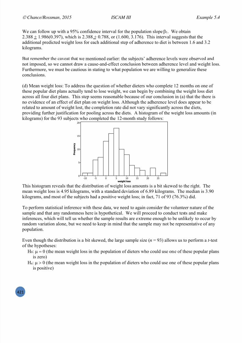
7/25/2019 Text: Investigating Statistical Concepts, Applications, and Methods
http://slidepdf.com/reader/full/text-investigating-statistical-concepts-applications-and-methods 422/428
Chance/Rossman, 2015 ISCAM III Example 5.4
P!W
We can follow up with a 95% confidence interval for the population slope 1. We obtain2.388 + 1.986(0.397), which is 2.388 + 0.788, or (1.600, 3.176). This interval suggests that theadditional predicted weight loss for each additional step of adherence to diet is between 1.6 and 3.2kilograms.
But remember the caveat tha t we mentioned earlier: the subjects’ adherence levels were obse rved andnot imposed, so we cannot draw a cause-and-effect conclusion between adherence level and weight loss.Furthermore, we must be cautious in stating to what population we are willing to generalize theseconclusions.
(d) Mean weight loss: To address the question of whether dieters who complete 12 months on one ofthese popular diet plans actually tend to lose weight, we can begin by combining the weight loss dietacross all four diet plans. This step seems reasonable because of our conclusion in (a) that the there isno evidence of an effect of diet plan on weight loss. Although the adherence level does appear to berelated to amount of weight lost, the completion rate did not vary significantly across the diets,
providing further justification for pooling across the diets. A histogram of the weight loss amounts (in
kilograms) for the 93 subjects who completed the 12-month study follows:
This histogram reveals that the distribution of weight loss amounts is a bit skewed to the right. Themean weight loss is 4.95 kilograms, with a standard deviation of 6.89 kilograms. The median is 3.90kilograms, and most of the subjects had a positive weight loss; in fact, 71 of 93 (76.3%) did.
To perform statistical inference with these data, we need to again consider the volunteer nature of thesample and that any randomness here is hypothetical. We will proceed to conduct tests and makeinferences, which will tell us whether the sample results are extreme enough to be unlikely to occur byrandom variation alone, but we need to keep in mind that the sample may not be representative of any
population.
Even though the distribution is a bit skewed, the large sample size ( n = 93) allows us to perform a t -testof the hypotheses:
H0: (the mean weight loss in the population of dieters who could use one of these popular plansis zero)
Ha: (the mean weight loss in the population of dieters who could use one of these popular plansis positive)
%#"&'$ )*++
; - # < 5 # / . 2
494359539369653
43
59
53
9
3

7/25/2019 Text: Investigating Statistical Concepts, Applications, and Methods
http://slidepdf.com/reader/full/text-investigating-statistical-concepts-applications-and-methods 423/428
Chance/Rossman, 2015 ISCAM III Example 5.4
P!!
The test statistic turns out to be to t 0 = 92.69389.6
095.4, producing a p-value of essentially zero. This
suggests that the sample data provide overwhelming evidence that the population mean weight lossexceeds zero, that is, that dieters on these plans do tend to lose weight on average. A 95% confidenceinterval for turns out to be (3.53, 6.36), so we can be 95% confident that the population mean weightloss is between 3.53 and 6.36 kilograms.
We can cautiously follow this up with a 95% prediction interval for the weight loss of an individual
dieter: 931
189.6986.195.4 , which is 4.95 + 13.76, which is ( 8.81, 18.71). This interval implies
that, with 95% confidence, we can assert only that an individual dieter is predicted to see a weightchange anywhere between a gain of 8.8 kilograms and a loss of 18.7 kilograms. However, the slightskewness in the sample data leads us to question the validity of this prediction interval because thenormality condition is essential for this procedure.
We could also perform a “sign test ” of the hypotheses. A sign test reduces the analysis to counting howmany “positive” and “negative” differences there are and determining whether we have significantlymore of one that then other.
H0: = 0.5 (half of the population of all potential dieters would lose positive weight on one of thesediet plans)
Ha: > 0.5 (more than half of the population of all potential dieters would lose positive weight on oneof these diet plans)
The data reveal that 71 of 93 subjects had positive weight loss. The binomial distribution (with parameters n = 93 and = 0.5) reveals that the p-value of P(X > 71) equals essentially zero ( z ≈ 5.08) .Thus, this sign test leads to a similar conclusion: overwhelming evidence that more than half of the
population would lose positive weight.
Because of the volunteer nature of the sample, it is not completely clear to what population we cangeneralize these results. Moreover, even though we concluded that the mean weight loss is significantlylarger than zero, we cannot attribute the cause to the diet. Without the use of a comparison group of
people who did not participate in a diet plan, we cannot conclude that the diet alone is responsible forthe tendency to lose weight. Perhaps even the power of suggestion from being in the study was asufficient cause for these individuals to lose weight on average.
Summarizing our findings from this study: We do not have convincing evidence to suggest that one of these popular diet plans produces
more weight loss on average than another.
We do not have convincing evidence to suggest that completion rates differ among the four diet plans.
We do have very strong evidence to suggest that dieters on one of these plans will lose weight, between 3.5 and 6.5 kg on average, subject to the caveat that the dieters in this study may not berepresentative of a larger population of overweight people.
We do have significant evidence that those who adhere to a diet more closely do tend to losemore weight (subject to the same caveat).

7/25/2019 Text: Investigating Statistical Concepts, Applications, and Methods
http://slidepdf.com/reader/full/text-investigating-statistical-concepts-applications-and-methods 424/428
Chance/Rossman, 2015 ISCAM III Chapter 5 Summary
P!#
).<9!/@ V 01BB<@_
In this chapter, you explored procedures for analyzing two or more groups and for analyzingrelationships. As in earlier chapters, you saw that different study designs could lead to the samemathematical computations, but also remember to consider the study design when drawing your final
conclusions. In particular, you should think about which variables were controlled by the researchersand which were not.
A very common procedure to use with two-way tables is the chi-square procedure. You saw that thisreduces to the two-sample z-test in the case of two groups. The chi-square procedure is a large sample
procedure and Fisher’s Exact Test can be used with smaller sample sizes. A parallel procedure forcomparing several means is Analysis of Variance, which models the ratio of the variability betweengroups to the variability within groups using the F distribution.
Regression is a very important field of study and your next course in statistics will probably be entirelyabout regression models. We scratched the surface here by looking at the appropriate numerical and
graphical summaries for analyzing the relationship between two quantitative variables (scatterplots andcorrelation coefficient) and least squares regression models for linear relationships. In deciding whetheryou have a statistically significant relationship, the t -statistic uses the common test statistic form thatyou saw in earlier chapters (observed – hypothesized)/standard error, where the standard error of thesample slopes depends on the sample size, the variability in the x values and the vertical spread aboutthe regression line.
These calculations are complex to carry out by hand, but our focus is on knowing when to use which procedure, how to check the validity of the procedure, and how to interpret the resulting output.Learning to effectively interpret and communicate statistical results is at least as important a skill aslearning which computer menus to use!
!/).3-K-N_ 01BB<@_ In this chapter, you learned how to use Minitab/R to perform chi-square tests, ANOVA, and
inference for regression. You also learned how to create scatterplots, including coded scatterplots,and calculate correlation coefficients.
You used applets to explore properties of F -statistics, regression lines, and regression coefficients.Though we hope these have given you some memorable visual images, you will generally use R orMinitab to carry out specific analyses.
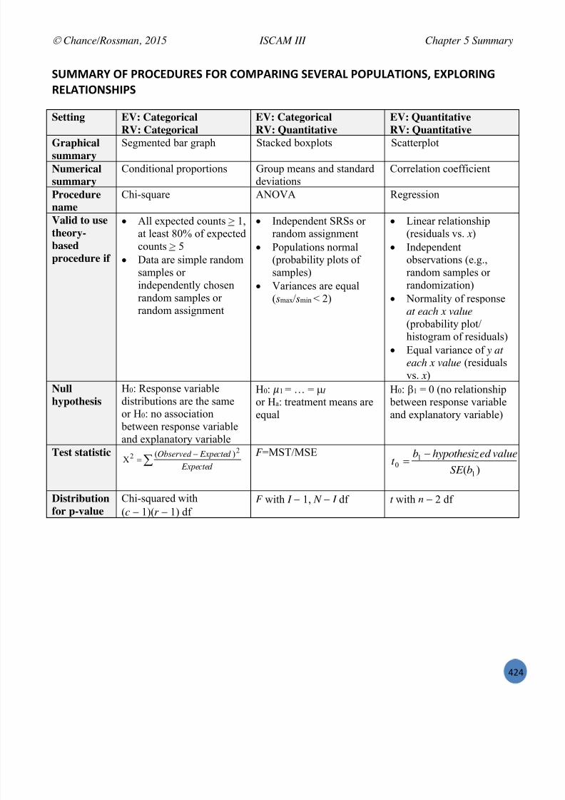
7/25/2019 Text: Investigating Statistical Concepts, Applications, and Methods
http://slidepdf.com/reader/full/text-investigating-statistical-concepts-applications-and-methods 425/428
Chance/Rossman, 2015 ISCAM III Chapter 5 Summary
P!P
01BB<@_ -L 9@-)/21@/0 L-@ )-B9<@M3N 0/J/@<K 9-91K<!M-30b /d9K-@M3N@/K<!M-30.M90
Setting EV: CategoricalRV: Categorical
EV: CategoricalRV: Quantitative
EV: QuantitativeRV: Quantitative
Graphicalsummary
Segmented bar graph Stacked boxplots Scatterplot
Numericalsummary
Conditional proportions Group means and standarddeviations
Correlation coefficient
Procedurename
Chi-square ANOVA Regression
Valid to usetheory-basedprocedure if
All expected counts > 1,at least 80% of expectedcounts > 5
Data are simple randomsamples orindependently chosenrandom samples orrandom assignment
Independent SRSs orrandom assignment
Populations normal(probability plots ofsamples)
Variances are equal(smax/smin < 2)
Linear relationship(residuals vs. x)
Independentobservations (e.g.,random samples orrandomization)
Normality of responseat each x value(probability plot/histogram of residuals)
Equal variance of y ateach x value (residualsvs. x)
Nullhypothesis
H0: Response variabledistributions are the sameor H0: no association
between response variableand explanatory variable
H0: 1 = … = I or H a: treatment means areequal
H0: 1 = 0 (no relationship between response variableand explanatory variable)
Test statistic Expected
Expected Observed 22 )( F =MST/MSE
)( 1
10 bSE
valueed hypothesizbt
Distributionfor p-value
Chi-squared with(c 1)(r 1) df
F with I 1, N I df t with n 2 df

7/25/2019 Text: Investigating Statistical Concepts, Applications, and Methods
http://slidepdf.com/reader/full/text-investigating-statistical-concepts-applications-and-methods 426/428
Chance/Rossman, 2015 ISCAM III Chapter 5 Summary
P!R
a487Q @%(%:%*7% +' M0)<B @ `':Q,?"7% L4*7+8'*, "*5 -+=%: @ )';;"*5,
9:'7%54:% 2%,8:%5 L4*7+8'* 3";% O-?+8'*,P]15*&- O51=&='-'%6 O-1% AA.15*F;&%&GO51=&='-'%6 O-1% AA8-1%F;&%& 951* ;'(%5'=2%'1.7 6125 ;&%&G
O51=&='-'%',( 951* N+':$A2&5, ;'(%5'=2%'1. '()&*)+'(A851=FB4&-7 ;9G5,%25.( 288,5 %&'- 851=&='-'%6
N+':(A2&5, I,(% )+'(A/%,(%F%&=-,F;&%&GG)+'(A/%,(%F%&=-,F;&%&GGe,B8,)%,; e5,(';2&-(
L.,:<&6 0]Lk0 (2**&56F&14F5,(81.(,q,B8-&.&%156GO51=&='-'%',( 951* Q ;'(%5'=2%'1. 89FB7 ;9W7 ;9!7 -1<,5/%&'-_Q0\$fG$)&%%,58-1% 8-1%F,B8-&.&%1567 5,(81.(,GN155,-&%'1. )1,99')',.% )15FB7 6G\,&(% $A2&5,( [,35,(('1. \'., -*F5,(81.(,q,B8-&.&%156G
-*F5,(1.(,q,B8-&.&%156Ge5,(';2&-(N1;,; $)&%%,58-1% 8-1%F5,(81.(,q,B8-&.&%1567 )1-_35128(G
@.9,5,.), 915 5,35,(('1. (2**&56F-*F5,(81.(,q,B8-&.&%156GGO5,;')%'1. '.%,54&-( 85,;')%F-*F5,(81.(,q,B8-&.&%156G7
.,<;&%&_;&%&/95&*,F,B8-&.&%156:4&-2,G7'.%,54&- _ `85,;')%'1.` 15 `)1.9';,.),`G
$28,5'*81(, * _ 5 -'., -'.,(F5,(81.(,7 5,(81.(,G$28,5'*81(, 5,35,(('1. -'., &=-'.,F-*F5,(81.(,q,B8-&.&%156GG
a487Q @%(%:%*7% +' B8*8+"# )';;"*5,
9:'7%54:% 2%,8:%5 B%*4O51=&='-'%6 O-1% b5&8+ a O51=&='-'%6 O-1%O51=&='-'%',( 951* N+':$A2&5, ;'(%5'=2%'1. b5&8+ a O51=&='-'%6 E'(%5'=2%'1. O-1%N+':(A2&5, I,(% $%&% a I&=-,( a N+':$A2&5, I,(% 915 0((1)'&%'1.
$%&% a I&=-,( a N51(( I&=2-&%'1. &.; N+':$A2&5,L.,:<&6 0]Lk0 $%&% a 0]Lk0 a L.,:<&6O51=&='-'%',( 951* Q ;'(%5'=2%'1. b5&8+ a O51=&='-'%6 E'(%5'=2%'1. O-1%$)&%%,58-1% b5&8+ a $)&%%,58-1%N155,-&%'1. )1,99')',.% $%&% a M&(') $%&%'(%')( a N155,-&%'1.\,&(% $A2&5,( [,35,(('1. \'., $%&% a [,35,(('1. a Q'%%,; \'., O-1%
$%15&3,? [,(';2&-(N1;,; $)&%%,58-1% b5&8+ a $)&%%,58-1%7 J'%+ b5128(@.9,5,.), 915 [,35,(('1. $%&% a [,35,(('1. a [,35,(('1. a Q'% [,35,(('1. C1;,-
O5,;')%'1. @.%,54&-( 09%,5 52..'.3 %+, *1;,-?$%&% a [,35,(('1. a [,35,(('1. a O5,;')%
$28,5'*81(, * _ 5 -'., 5'3+% )-')>7 0;; a N&-)2-&%,; \'.,$28,5'*81(, 5,35,(('1. -'., $%&% a [,35,(('1. a Q'%%,; \'., O-1%
5'3+% )-')> 1. ()&%%,58-1%7 0;; a [,35,(('1. Q'%

7/25/2019 Text: Investigating Statistical Concepts, Applications, and Methods
http://slidepdf.com/reader/full/text-investigating-statistical-concepts-applications-and-methods 427/428
Chance/Rossman, 2015 ISCAM III Index
P!S
M32/d
Addition rule, 16Adjusted Wald interval, 90Alternative hypothesis, 37ANOVA, 342Applet
Analyzing two quantitative variables, 368,389
Analyzing two-way tables, 217, 331Comparing groups (quantitative), 277, 341,
346Dolphin study, 213Guess the Correlation, 363Matched pairs randomization, 294
Normal probability calculator, 73, 83One proportion inference, 23, 41Power simulation, 55Random Babies, 13Randomizing subjects, 204Reese's Pieces, 66Sampling from finite population, 151Sampling words, 104Simulating ANOVA tables, 350Simulating confidence intervals, 86, 93Theory-Based inference, 79
Bar graph, 20, 33
Baseline rate, 226Basic regression model, 392Biased, 97Binary, 36Binomial distribution, 27Binomial intervals, 50Binomial power, 63Binomial probabilities, 34Binomial rejection region, 62Binomial test, 38Blinding (experiment), 208
Boxplot, 144Case-control study, 234Categorical, 36Center of distribution, 139Central limit theorem
sample proportion, 69, 106Central Limit Theorem
difference in proportions, 191Chi-square distribution, 324Chi-square test statistic, 322Coefficient of determination, 372Cohort study, 234Comparative experiment, 208Comparing two proportions, 195Complement rule, 16Conditional proportions, 186Confidence interval, 49Confidence level, 87Confounding variables, 198Continuity correction, 78Convenience sample, 97Correlation coefficient, 359Coverage rate, 87Critical value, 84Cross-classified study, 234Cross-sectional design, 234Distribution, 138Double blind, 208Duality, 51Exact binomial inference, 53Expected value, 16, 43Experimental study, 202
Experimental units, 202Explanatory variable, 196Extrapolation, 372F distribution, 342F statistic, 342Finite population correction factor, 113Fisher's exact test, 219Hawthorne effect, 208Homogeneity of proportions, 326Hypergeometric distribution, 217, 218hypergeometric random variable, 112
Hypotheses, 37Hypothesized value, 49Independence, 28Influential observation, 380Intercept coefficient, 371Interquartile range, 143Interquartile range (IQR), 144
7/25/2019 Text: Investigating Statistical Concepts, Applications, and Methods
http://slidepdf.com/reader/full/text-investigating-statistical-concepts-applications-and-methods 428/428
Chance/Rossman, 2015 ISCAM III Index
Least squares line, 369Least squares regression line, 369Level of significance, 55Linear association, 356Long-run proportion, 13
Margin-of-error, 84Matched-pairs design, 288Mean of absolute differences (MAD), 346Mutually exclusive, 28
Negative association, 356 Non-sampling errors, 108 Normal approximation to binomial, 79 Normal probability calculations, 72 Normal probability curve, 68 Null distribution, 21 Null hypothesis, 37
Null model, 21Observational study, 202Observational units, 36Odds, 234Odds ratio, inference, 238One proportion z-intervals, 85One proportion z-procedures, 116One proportion z-test, 81One sample t -test, 163One sample z-interval, 84One-sided alternative, 45Outlier, 144Paired data, 290Paired t -procedures, 300Paired t -test, 295Parallel dotplots, 137, 258, 290Parallel histograms, 138
p-value, 24Quantitative, 36Random assignment, 203Random variable, 15Randomization test, 277, 278
Randomized experiment, 208Regression line, 369Rejection region, 55Relative frequency, 13 Relative risk, 226Relative risk, inference, 231Residual, 332, 343, 366Residual plots, 393Response variable, 196Retrospective design, 234Sample, 95
Sample size, 36Sampling frame, 98Sampling variability, 97Scatterplot, 355Scope of conclusions, 25Segmented bar graphs, 186Shape of distribution, 138Sign test, 422Significance, 24Simple random sample, 97Simple random sample, selecting, 98, 260Skewed distributions, 138Skewed to the left, 138Skewed to the right, 138Slope coefficient, 371Spread. See VariabilitySquared residuals, 367, 369