Application of Geotechnical Data toResource Planning in Southeast Alaska

United States Department of Agriculture Forest Service

Pacific Northwest Research Station

General Technical Report PNW-198 January 1987

W.L. Schroeder and Douglas N. Swanston

This file was created by scanning the printed publication. Text errors identified by the software have been corrected;

however, some errors may remain.

W.L. SCHROEDER is professor of geotechnical engineering, Oregon State Univer-sity, Civil Engineering Department, Corvallis, Oregon 97331. DOUGLAS N. SWANSTON is principal research geologist, Pacific Northwest Research Station, Forestry Sciences Laboratory, P.O. Box 909, Juneau, Alaska 99802.

Authors

Abstract Schroeder, W.L.; Swanston, Douglas N. Application of geotechnical data to resource planning in southeast Alaska. Gen. Tech. Rep. PNW-198. Portland, OR: U.S. Department of Agriculture, Forest Service, Pacific Northwest Research Sta-tion; 1987. 22 p.

Recent quantification of engineering properties and index values of dominant soil types in the Alexander Archipelago, southeast Alaska, have revealed consistent diagnostic characteristics useful to evaluating landslide risk and subgrade material stability before timber harvesting and low-volume road construction. Shear strength data are summarized and grouped by Soil Conservation Service soil series, by the Unified Soil Classification system, and by geologic origin. Such groupings allow the selection of strength parameters for slope and subgrade stability analyses based on existing knowledge of the terrain and on available inventory data. Parameters are expressed by mean and minimum values so that both average and conserv-ative evaluations can be made, depending on management requirements. Engineering procedures were used to incorporate the parameters into planning and project-level investigations to identify areas of unstable terrain, to assess levels of landslide risk, and to define suitability of materials for road construction.

Keywords: Slope stability, subgrade stability, soil properties (physical), southeast Alaska, Alaska (southeast).

Contents 1 Introduction

2 The Developing Data Base

3 Required Data

13 Analysis

16 Combining Reconnaissance and Analysis

17 Road Subgrades and Bases

21 Conclusions

21 Metric Equivalents

22 Literature Cited

Introduction Slope failures in coastal Alaska occur primarily as debris avalanches in shallow hillslope depressions. The susceptibility of such sites to failure is a function of slope gradient, overburden depth, 1/ soil strength, and the soil's ability to absorb and transmit water. A controlling factor in almost all failures is the development of a temporary water table in these depressions during high-intensity, long-duration rainfall. Positive porewater pressures generated by this subsurface water reduce soil effective stresses 2/ within the depressions and may either directly initiate a landslide or render the site susceptible to failure during some external loading event, such as windthrow or rockfall.

Timber harvesting in coastal Alaska usually requires construction of access and haul roads. These roads must be built in unfavorable circumstances: weather and soil moisture conditions are poor throughout the year, and freezing is often a pos-sibility; many roads are built on muskeg that, during normal construction, would be removed or avoided; and access for equipment is costly and difficult. In spite of these problems, roads are being built, and planning for the roads must be based on available information on using naturally occurring vs. imported soil and rock.

This paper discusses the developing geotechnical and hydrological data bases and shows how the information, coupled with simplified engineering analysis procedures, can be used in resource allocation and project planning studies. Techniques are suggested for analyzing natural slopes using the infinite slope method and for analyzing slopes created by road cuts using an approximate circular arc procedure. These techniques are fairly well developed. Only general guidelines for using natural materials for roadway construction are given.

Results of analyses are intended only for resource allocation and for planning studies. Stability evaluations for specific sites and subgrade strength analyses re-quire detailed, site-specific investigations.

1/Overburden depth refers to the residual and colluvial soils and organic debris overlying bedrock and dense glacial till.

2/ Effective stress is a force per unit area that tends to cause compression or deformation of the solid phase of the soil. In this case, the effective stress is due to the weight of the solid in the depressions exerted along an impermeable bedrock or glacial till surface.

1

The Developing Data Base

2

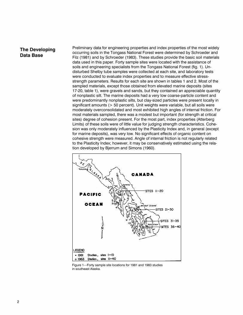
Preliminary data for engineering properties and index properties of the most widely occurring soils in the Tongass National Forest were determined by Schroeder and Filz (1981) and by Schroeder (1983). These studies provide the basic soil materials data used in this paper. Forty sample sites were located with the assistance of soils and engineering specialists from the Tongass National Forest (fig. 1). Un-disturbed Shelby tube samples were collected at each site, and laboratory tests were conducted to evaluate index properties and to measure effective stress-strength parameters. Results for each site are shown in tables 1 and 2. Most of the sampled materials, except those obtained from elevated marine deposits (sites 17-20, table 1), were gravels and sands, but they contained an appreciable quantity of nonplastic silt. The marine deposits had a very low coarse-particle content and were predominantly nonplastic silts, but clay-sized particles were present locally in significant amounts (> 50 percent). Unit weights were variable, but all soils were moderately overconsolidated and most exhibited high angles of internal friction. For most materials sampled, there was a modest but important (for strength at critical sites) degree of cohesion present. For the most part, index properties (Atterberg Limits) of these soils were of little value for judging strength characteristics. Cohe-sion was only moderately influenced by the Plasticity Index and, in general (except for marine deposits), was very low. No significant effects of organic content on cohesive strength were measured. Angle of internal friction is not regularly related to the Plasticity Index; however, it may be conservatively estimated using the rela-tion developed by Bjerrum and Simons (1960).

Figure 1––Forty sample site locations for 1981 and 1983 studies in southeast Alaska.

3

Table 1––Results of indexed property tests of undisturbed southeast Alaska forest soils, by site number

A wide variety of material was sampled. Variability in test results between types and even within types of material was great and made strict comparisons difficult. There were, however, enough similarities in engineering characteristics to allow reasonable groupings by (1) Soil Resource Inventory series, (2) Unified Soil Clas-sification system (USC), and (3) geologic origin designations (tables 3, 4, and 5, respectively). Because of difficult logistics and the large geographic area sampled, the number of samples for each grouping was not large (minimum 4, maximum 7); statistical evaluation of the data therefore has limitations. The data do, however, provide estimates of properties and their range within groupings. The mean and the fifth percentile of soil strength variables for each grouping were estimated using laboratory test results (tables 6, 7, and 8). The fifth percentile is the value such that 5 percent of the values of a normally distributed sample population are less than this. The normal distribution of these engineering properties has been demonstrated in the Pacific Northwest under similar geomorphic and climatic con-ditions (Schroeder and Alto 1983). The fifth percentile therefore represents a reasonable estimate of a minimum property value. The mean values may be used for general assessment of soil behavior; the fifth percentile should be used in sen-sitive situations where the consequences of occasional failures are especially undesirable.

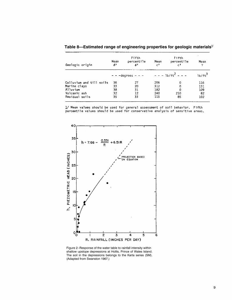
Hydrologic data have been quantified for only a few critical areas, but the general relations to site stability are known. Existing data can be used effectively to estimate the influence of storms on slope stability for planning-level risk assess-ment. Swanston (1967) developed initial data on ground-water level fluctuations in permeable materials within shallow upslope depressions at Hollis, Prince of Wales Island, and related them to 24-hour rainfall intensities. The materials were Karta soils (which classify as SM soils by the USC system) derived from the weathering of glacial tills. These soils have a low content of nonplastic silt and consequently exhibit high permeabilities. The characteristics of these materials are represented by sites 3 and 8 in table 1. Because of the high permeabilities, the response of water table level to rainfall intensity is rapid. The relation between ground-water height (h in inches) and 24-hour rainfall intensity (R in inches per day) is curvi- linear (fig. 2) and is expressed by the equation:

h = 7.66 - 0.331 + 6.51R . R

(1)

As rainfall intensity increases, water level rises rapidly at first, but at a decreasing rate as rainfall continues, and reaches an upper limit determined by the thickness of the soil profile.

More detailed work in progress at Kennel Creek on Chichagof Island (Sidle in press,Sidle and Swanston 1980, 1981) indicates a similar general response of degree of saturation to rainfall intensity for less pervious materials in the Kupreanof Series (SM-MH soils in the USC system) (sites 23 and 26 in table 2). The response ap-pears, however, to be much more closely related to maximum 2-hour rainfall inten-sity, antecedent 24-hour rainfall, and duration of a storm.

4

5

Table 2 ––Results of consolidated, undrained triaxial shear tests of undisturbed southeast Alaska forest soils, by site number

6

Table 3––Samples grouped by Soil Resource Inventory (SRI) soil type

Table 4––Samples grouped by Unified Soil Classification (USC) soil type

7

Table 5––Samples grouped by geologic origin

8

Table 7––Estimated range of engineering properties for Unified Soil Classifica-tion (USC) soil types1/

Table 6––Estimated range of engineering properties for Soil Resource Inven-tory (SRI) soil types 1/

.

9

Table 8––Estimated range of engineering properties for geologic materials1/

Figure 2--Response of the water table to rainfall intensity within shallow upslope depressions at Hollis, Prince of Wales Island. The soil in the depressions belongs to the Karta series (SM). (Adapted from Swanston 1967.)

Landslide Risk Analysis Procedures

Required Data

10

Prellwitz (1985) recommends a three-level approach to landslide risk analysis. Each successive level requires a more detailed look at the potential for mass instability. Briefly described, Prellwitz’ recommended analysis levels include the following:

Level I––Resource allocation; provides managers with an overview of landslide potential that is adequate for resource allocation planning.

Level II––Project planning; predicts response of slide-prone areas to various harvesting systems and transportation routes.

Level III––Critical site stabilization; evaluates stabilization techniques at critical sites before and after any construction.

Figure 3 gives a general outline for any landslide risk assessment. Elements of it can be incorporated in either a level I or a level II analysis; either analysis requires topographic mapping and geologic reconnaissance studies. The geologic recon-naissance study identifies bedrock and structural control in an area, defines limiting characteristics of terrain and materials, and delineates areas where mass movement historically has been a problem. In level I studies, these areas usually are designated as "high-risk zones" and are avoided in resource allocation plans or are identified for more intensive evaluation. Soil properties usually are not quan- tified nor are engineering analyses made. Risk assessment is based largely on an inductive evaluation of the area, which is based on observation. In level II studies, more specific site investigations are incorporated to identify critical zones of in- stability and to provide a way to determine where cutting units and roads will be located.

The engineering methods presented here supplement the experience-based assessment procedures commonly used for resource allocation planning. The methods provide an analytical approach to identify a range of risk levels within apotentially troublesome area and to assign criteria for efficient and effective management.

Data required to use the objective analysis method include:

1. Slope data––natural slope angle and the slope angle and height of the road cut. These are obtained from topographic maps, field measurements, and preliminary construction plans.

2. Ground-water levels––location of the ground-water surface during critical periods. In southeast Alaska this is usually between September and December. Swanston's (1967) analysis of ground-water fluctuations in response to 24-hour rainfall inten-sities for shallow, permeable soils is shown in figure 2. To use figure 2, it is neces-sary to determine, for the location of landslide risk assessment, a rainfall associated with the project requirements. Isohyte maps of 24-hour rainfall intensity for different recurrence intervals in southeast Alaska were plotted by Miller (1963). An example for a 10-year recurrence interval is shown in figure 4.

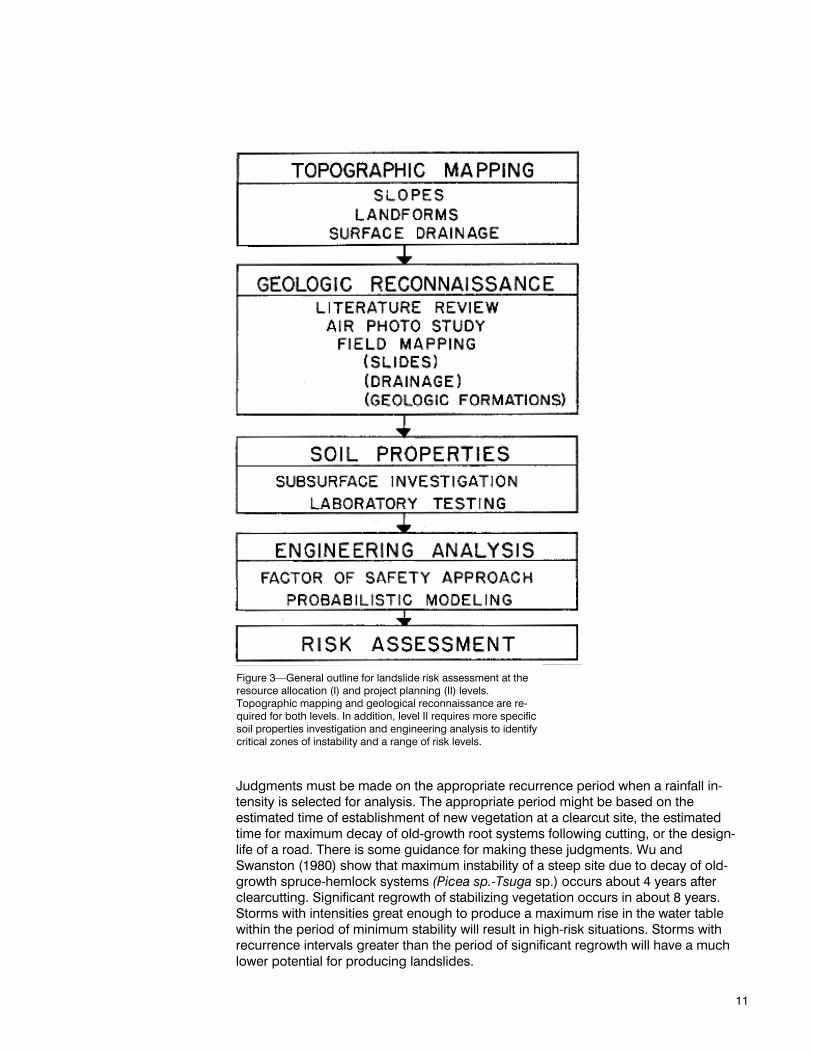
Figure 3––General outline for landslide risk assessment at the resource allocation (I) and project planning (II) levels. Topographic mapping and geological reconnaissance are re-quired for both levels. In addition, level II requires more specific soil properties investigation and engineering analysis to identify critical zones of instability and a range of risk levels.

Judgments must be made on the appropriate recurrence period when a rainfall in-tensity is selected for analysis. The appropriate period might be based on the estimated time of establishment of new vegetation at a clearcut site, the estimated time for maximum decay of old-growth root systems following cutting, or the design-life of a road. There is some guidance for making these judgments. Wu and Swanston (1980) show that maximum instability of a steep site due to decay of old-growth spruce-hemlock systems (Picea sp.-Tsuga sp.) occurs about 4 years after clearcutting. Significant regrowth of stabilizing vegetation occurs in about 8 years. Storms with intensities great enough to produce a maximum rise in the water table within the period of minimum stability will result in high-risk situations. Storms with recurrence intervals greater than the period of significant regrowth will have a much lower potential for producing landslides.

11

Figure 4–– Ten-year recurrence interval, 24-hour rainfall pattern for southeast Alaska, in inches (Miller 1963).

The piezometric head on the y-axis of figure 2 is the water level above an imper-vious subsurface. Soil depth above this impervious surface must also be known to do a stability analysis. In the typically shallow soils found at unstable sites in south-east Alaska, soil depth can be obtained readily by using probes or augers. For deeper soil sites or where large quantities of rock are entrained in the overburden profile, a seismograph can be used. For level I (planning) analyses, estimates of soil depth based on Soil Resource Inventory (SRI) maps are usually adequate.

3. Data on soil properties are summarized in tables 6, 7, and 8. Any of these tables can be used to assign soil properties for analysis according to terrain infor-mation available to the user. In the tables, mean soil shear strength variables (φ') and (c'), and bulk (saturated) unit weights (γ) are given. Also shown are more con-servative (fifth percentile) values of the shear strength parameters. The minimum values are derived by subtracting two standard deviations from the mean parameter to obtain an approximate lower 95-percent confidence limit. By this method, the parameter indicated represents, approximately, the lower strength limit for 95 per-cent of the soil group. The accuracy of these lower limits can be only approximated because of the small number of samples in each soil group. Where better data are available, or where individual sites have been identified for further project level analysis, the user should develop and assign more appropriate soil strength parameters. In level II site investigations, particular care should be taken when directly applying these assigned values. Natural variation in soil properties and structural weaknesses (for example, the presence of a weak layer at the soil/rock interface) may result in overestimation of material strength.

12

Analysis This section explains the recommended procedures for level I or level II analysis (refer to fig. 3). A geologic reconnaissance is desirable at both levels to define con-trolling terrain characteristics and to identify those areas with a history of active landsliding. In addition, site investigations should be conducted in identified critical areas for level II to facilitate location of final cutting unit boundaries and road cor-ridors. The investigations should include, at a minimum, preparation of field-developed cross sections and collection of data on site-specific soil properties and structure. Step-by-step procedures are:

1. Obtain a topographic map of the study area.

2. Prepare an overlay map of the slopes in the study area using convenient slope ranges; suggested ranges are 0-30 percent, 30-50 percent, 50-60 percent, and more than 60 percent.

3. Identify areas with a history of active landsliding by using aerial photographs, ground reconnaissance, or available landslide inventories.

4. Identify dominant soil types and depths for each portion of the study area within each slope range selected in step 2. Choose strength parameters, φ’, and c', and a bulk unit weight, γ, from tables 1, 2, or 3. Mean values normally are used, but minimumvalues may be chosen for especially sensitive areas.

5. Select the recurrence interval for the 24-hour rainfall to be used in the stability assessment. Research has shown that landslide frequency is greatest in clearcut- tings 3 to 5 years after logging (Swanston 1974). Conservative estimates of land- slide risk could, therefore, be based on a 10-year recurrence interval; less conservative estimates could be based on a 5-year return interval.

6. Determine, from figure 2, the estimated ground-water height (piezometric head), h, for the selected 24-hour rainfall.

7. Use simplified engineering procedures and estimated or field-developed strength parameters to determine the potential instability of natural slopes and slopes created by cuts for roads.

Natural slopes––Use equation (2), the infinite slope equation, to compute the factor of safety (FS) for various slope classes:

(2)

In equation (2), c', φ’. and γ are taken from tables 6, 7, or 8. The soil depth is z. If h is the ground-water height from step 6, above, then m = h/z. The unit weight of water, γw, is 62.4 pounds per cubic foot (lb/ft3). Other units may be used in equa-tion (2), but all units must be dimensionally consistent. Slope angle, in degrees, is represented by β, which is equal to the angle whose tangent is the percent of the slope divided by 100.

13

Cut slopes––Slopes caused by cuts made for roads are presumed to be stable at the time of excavation. In special cases, where previously existing landslides are transected by a cut, this would not necessarily be true. For purposes of risk analysis, such areas would be identified in the geologic reconnaissance phase and be assessed separately. Typically, cut slopes become unstable during the rainy season.

In addition to steps 1-6, above, it is necessary to know the proposed angle (β) of the cut slope and the slope height to compute the relative stability of proposed cut slopes. For logging roads, a proposed cut slope angle is estimated and height limits for the slope are chosen based on roadway width requirements, road align-ment, and topography.

For cohesion less soils (c' = 0), the factor of safety is computed using equation (2). The first term is set equal to zero and β is set equal to the angle of the cut slope above the horizontal. For cohesive soils, calculations are based on the method illustrated in figure 5.

Examples––Suppose the impact on slope stability from roads and from logging a watershed in the upper elevations of northern Chichagof Island must be estimated. A geologic reconnaissance of the watershed has been completed by using aerial photographs and limited ground reconnaissance. There are no significant bedrock exposures. The dominant soil type is a weathered glacial till with an average depth of 6 feet. The overlay map of the slopes has been completed, and it shows the following distribution of natural slope classes:

Slope class Slope angle Percent of watershed area

From table 8, the following soil properties are selected:

φ‘' (mean) = 36° c ' (mean) = 206 pounds per square foot (lb/ft2) γ ’ (mean) = 116 pounds per cubic foot (lb/ft3) φ’’ (minimum) = 27° c ' (minimum) = 0 pounds per square foot (lb/ft2)

For a 10-year recurrence interval, the estimated 24-hour rainfall is 10 inches (from fig. 4). From figure 2, for a projection of 10 inches of rainfall per day in drainage depressions, h = 73 inches or about 6 feet. Therefore m = 1. For natural slopes and under average conditions, from equation (2):

14

0-30 percent30-50 percent50-60 percent> 60 percent

0-16.7°16.7-26.6°

26.6-31 °>31 °

265218

4

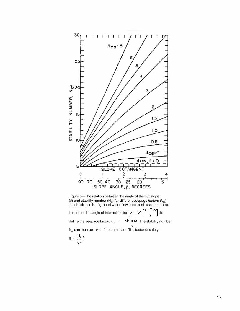
Figure 5––The relation between the angle of the cut slope (β) and stability number (Ncf) for different seepage factors (λcφ) in cohesive soils. If ground water flow is present, use an approx-

15

imation of the angle of internal friction ,to define the seepage factor, λcφ = The stability number, Ncf can then be taken from the chart. The factor of safety Is =

Combining Reconnaissance and Analysis

For the various slope classes, the range in the factor of safety (FS) would be:

Slope class Percent of watershed area FS S _

0-30 percent30-50 percent50-60 percent> 60 percent

265218

4

Very high-2.202.20-1.411.41-1.23

<1.23

Now consider the proposed roads in the watershed. Preliminary plans indicate that the cuts for roads will be as high as 15 feet and that the slope inclination will be 1/2 (horizontal):1 (vertical). Previously selected soil properties are applicable, as is the water level resulting from rainfall infiltration for the 10-year, 24-hour rainfall.

First, (3 = arc tan (2) = 63.4°. Because of the heavy downslope seepage, an ap-proximation must be made for φ to use figure 5:

which leads to:

Note that the soil depth, z, is less than the full depth of the cut. Therefore, the cut height, H, is equal to z, or 6 feet. Then from figure 5, Net = 6.3 and:

The result indicates that the soil mantle over rock in the deepest proposed cuts would be stable (FS >1) and would have an adequate (>1.5) factor of safety.

The areas with greatest landslide risk are those where landslides have happened before, where analysis indicates they should happen again, and where there will be unacceptable consequences if they do happen. The areas with least risk are those where there have been no slides, where analysis shows that there should not have been slides, and where the consequences would be tolerable if there were slides. In between these limits there is a gradation of risk that can be as-signed according to criteria listed in table 9.

The descriptions "low," "moderate," and "high" are subjective only. Risk levels can also be quantified based on probability. To do so requires a large data base to determine confidence in parameters for soil shear strength and in ground-water response to rainfall. Because this data base is not presently available for south- east Alaska, we did not quantify risk based on probability.

16

(4)

(3)

(5)

Road Subgrades and Bases

Table 9––Supplemental criteria for assessing the risk of landslides

To use table 9, begin with the landslide history and use data from ground recon-naissance or aerial photographs. If the area under consideration has frequent land-slides or is presently involved in active sliding, if the calculated factor of safety is less than 1.25, and if a new slide would produce unacceptable consequences, the area is a high-risk area. It should be avoided, or the risks should be reduced in some way. For other, less well-defined situations, judgments must be made con-cerning weights to be assigned to each criterion in table 9 to arrive at an overall risk level. For instance, in an area with no landslide history (low risk), where the calculated factor of safety is 1.3 (moderate risk), and where the consequences of an actual slide are tolerable (low risk), an activity capable of triggering a slide could probably be done without great risk.

In our hypothetical watershed on Chichagof Island, there was no notable landslide history and no especially sensitive areas to be affected by landslides. The stability analysis for natural slopes indicates, according to table 9, that clearcutting on slopes up to about 50 percent would be generally acceptable and should not pro-duce significant sliding in the cut units. The risk goes up as slopes approach 60 percent but is still generally acceptable. Slopes steeper than 60 percent should not be logged. The analysis therefore indicates, based on slope stability risks, that up to 96 percent of the watershed may be cut. The leave areas should be shown on the overlay map. Slopes adjacent to proposed roads in the watershed should be stable. The analysis cannot be interpreted to mean that there would be no slides in the cut units and along roads because all slide-susceptible areas, of course, may not be adequately represented in the data base.

Costs for timber access and haul roads in southeast Alaska vary dramatically ac-cording to the suitability of onsite materials for roadway construction. Most road building in the Alaska Region (of the USDA Forest Service) requires development of offsite quarries, and transport costs can be very high. Quarry development may result in a major environmental impact. Where materials from within the road align-ment can be used for construction, both dollar savings and aesthetic benefits result. In a few areas, depending on joint spacing and construction methods, ex-cavations can be used for fill. Unfortunately, on steep ground it is difficult to blast rock small enough for fill and to keep it at the site.

17

Surfacing for roads requires good quality material. In southeast Alaska surfacing usually comes from natural materials that most often consist of pit run, screened, or crushed quarry rock. Asphalt and concrete surfacing are seldom used. The re-quired thickness of rock varies according to the strength of the underlying subgrade materials. Conditions throughout southeast Alaska are generally poor for road construction. The wet climate, the predominance of soils with considerable fines content, and the standard practices currently followed by the road building in-dustry result in circumstances that make quality road construction difficult, at best. Rather than building conventional roads on compacted subgrades with thin layers of base materials (less than 16 inches), subgrade reinforcement to depths ranging from 2 to 10 feet is needed to support vehicles.

Tables 1 and 4 provide Unified Soil Classification (USC) designations for soils represented in the data base. Table 4 relates these classes to both soil series and geologic origin. The classes of soils to be expected in a given management area can be forecast from geology and soil survey maps.

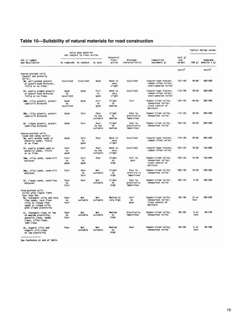
Table 10 ranks soils for road construction purposes according to their Unified Soil Classification designation; the ranking runs from highest quality to lowest. Table 4 is arranged the same way. Base course-type materials usually serve as the road surface. It is beyond the scope of this paper to provide design criteria for surface thickness of Forest Service roads. Such designs are more properly handled by regional or area engineering staffs. However, this section provides the basis for a general assessment of the suitability of natural materials for road construction. Such an assessment is consistent with the level of definition provided by landslide risk analysis at level I or level II (Prellwitz 1984).

Consider, for example, the hypothetical watershed on northern Chichagof Island that was discussed earlier. The area is underlain predominantly by weathered glacial tills. Table 4 shows that these are typically coarse soils, usually gravels, with considerable plastic fines. Table 1 indicates that fines content might range between about 20 and 50 percent.

Table 10 shows that weathered glacial tills would be good subgrade materials, even if subject to frost action, but they contain too much fine material to be suitable for a base course beneath a paved surface or a wearing surface. Further, the high fines content does not allow good drainage and, in the climate of southeast Alaska, probably makes such soils difficult to compact and to work with equipment during most of the year. A road constructed on these materials would require an im-ported surfacing.

The foregoing example considers the expected suitability of onsite road building materials in one of the higher quality (upper portion of table 4) materials in the data base. The evaluation indicates that properly placed and compacted, the material is good as a subgrade; however, actual field conditions are likely to work against good construction practices. Timber access and haul road construction in south-east Alaska usually will be difficult and expensive because other materials are of typically lower quality.

18

19

Table 10—Suitability of natural materials for road construction

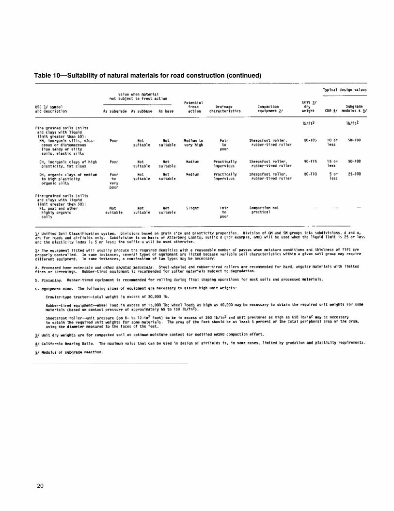
Table 10—Suitability of natural materials for road construction (continued)

20

Conclusions

Metric Equivalents

Extensive quantification of geotechnical information on surficial materials in southeast Alaska is lacking. A data base is developing, however, that links engineering properties and index values to dominant soil types as designated and mapped by the USDA Forest Service, Alaska Region, Soils Resource Inventory. This information, coupled with simplified engineering analysis procedures, can be used in resource allocation and project planning analyses to determine the poten-tial instability of natural slopes and of slopes created by cuts for roads. The infor-mation is also useful for assessing the suitability of these soils as road subgrades and bases.

1 inch (in) = 2.54 centimeters (cm) 1 foot (ft) = 0.31 meter (m) 1 mile (mi) = 1.61 kilometers (km) 1 pound-mass (lb) = 0.45 kilogram mass 1 square inch (in2) = 6.47 square centimeters (cm2) 1 square foot (ft2) = 0.09 square centimeter (cm2) 1 cubic inch (in3) = 16.39 cubic centimeters (cm3) 1 cubic foot (ft3) = 0.03 cubic meter (m3) 1 pound-force (Ibf) = 4.45 newtons (N) 1 pound-force per square inch (lbf/in2) = 0.07 kilogram-force per square centimeter (kgf/cm2) 1 pound-mass per cubic inch (lb/in3) = 27680.0 kilograms-mass per square meter (kg/cm3) 1 pound-force per square foot (lbf/ft2) = 4.88 kilograms-force per square meter (kgf/m2) 1 pound-mass per cubic foot (lb/ft3) = 16.02 kilograms-mass per cubic meter (kg/m3)

21

Literature Cited

22

Bjerrum, L.; Simons, N.E. Comparison of shear strength characteristics of nor- mally consolidated clays. In: Proceedings, Specialty conference on shear strength of cohesive soils; [date of conference unknown]; [location of conference unknown]. [Location of publisher unknown]: American Society of Civil Engineers; 1960: 711-726.

Miller, John. Probable maximum precipitation and rainfall frequency data for Alaska. Tech. Pap. 47. Washington, DC: U.S. Department of Commerce, En-vironmental Science Services Administration, Weather Bureau; 1963. 69 p.

Prellwitz, R.W. A complete three-level approach for analyzing landslides on forest lands. In: Proceedings, A workshop on slope stability--problems and solutions in forest management; 1984 January 6-8; Seattle, WA. Gen. Tech. Rep. 180. Portland, OR: U.S. Department of Agriculture, Forest Service, Pacific Northwest Forest and Range Experiment Station; 1985: 94-98.

Schroeder, W.L. Geotechnical properties of southeast Alaskan forest soils. Cor- vallis, OR: Oregon State University, Civil Engineering Department; 1983. 46 p.

Schroeder, W.L.; Alto, J.V. Soil properties for slope stability analysis: Oregon and Washington coastal mountains. Forest Science. 29(4): 823-833; 1983

Schroeder, W.L.; Filz, G. Engineering properties of southeast Alaska forest soils. Corvallis, OR-: Oregon State University, Civil Engineering Department; 1981.

51 p.

Sidle, R.C. Shallow groundwater fluctuations in unstable hillslopes in coastal Alaska. Zeitschrift fur Gletscherkunde und Glazialgeologie. [In press].

Sidle, R.C.; Swanston, D.N. Groundwater response to rainfall in shallow upslope depressions of coastal Alaska. Transactions of the American Geophysical Union. 61(46): 960; 1980. Abstract.

Sidle, R.C.; Swanston, D.N. Storm characteristics affecting piezometric rise in unstable hillslopes of southeast Alaska. Transactions of the American Geophysical Union. 62(45): 856; 1981. Abstract.

Swanston, D.N. Soil-water piezometry in a southeast Alaska landslide area. Res. Note PNW-68. Portland, OR: U.S. Department of Agriculture, Forest Service, Pacific Northwest Forest and Range Experiment Station; 1967. 17 p.

Swanston, D.N. The forest ecosystem of southeast Alaska. 5: Soil mass move-ment. Gen. Tech. Rep. PNW-17. Portland, OR: U.S. Department of Agriculture, Forest Service, Pacific Northwest Forest and Range Experiment Station; 1974. 22 p.

Wu, T.H.; Swanston, D.N. Risk of landslides in shallow soils and its relation to clearcutting in southeastern Alaska. Forest Science. 26(3): 495-510; 1980.

Schroeder, W.L.; Swanston, Douglas N. Application of geotechnical data to resource planning in southeast Alaska. Gen. Tech. Rep. PNW-198. Portland, OR: U.S. Department of Agriculture, Forest Service, Pacific Northwest Research Sta-tion; 1987.22 p.

Recent quantification of engineering properties and index values of dominant soil types in the Alexander Archipelago, southeast Alaska, have revealed consistent diagnostic characteristics useful to evaluating landslide risk and subgrade material stability before timber harvesting and low-volume road construction. Shear strength data are summarized and grouped by Soil Conservation Service soil series, by the Unified Soil Classification system, and by geologic origin. Such groupings allow the selection of strength parameters for slope and subgrade stability analyses based on existing knowledge of the terrain and on available inventory data. Parameters are expressed by mean and minimum values so that both average and conserv-ative evaluations can be made, depending on management requirements. Engineering procedures were used to incorporate the parameters into planning and project-level investigations to identify areas of unstable terrain, to assess levels of landslide risk, and to define suitability of materials for road construction.

Keywords: Slope stability, subgrade stability, soil properties (physical), southeast Alaska, Alaska (southeast).

The Forest Service of the U.S. Department of Agriculture is dedicated to the principle of multiple use management of the Nation's forest resources for sustained yields of wood, water, forage, wildlife, and recreation. Through forestry research, cooperation with the States and private forest owners, and management of the National Forests and National Grasslands, it strives––as directed by Congress––to provide increasingly greater service to a growing Nation.

The U.S. Department of Agriculture is an Equal Opportunity Employer. Applicants for all Departmentprograms will be given equal consideration without regard to age, race, color, sex, religion, or national origin.

Pacific Northwest Research Station 319 S.W. Pine St. P.O. Box 3890 Portland, Oregon 97208

U.S. Department of Agriculture Pacific Northwest Research Station 319 S.W. Pine Street P.O. Box 3890 Portland, Oregon 97208

BULK RATE POSTAGE + FEES PAID USDA-FS

PERMIT No. G-40

Official Business Penalty for Private Use, $300

do NOT detach label