Embed Size (px)
Citation preview

i
Wayne E. Etter
Professor
Department of Finance
and
Real Estate Center
Texas A&M University
College Station, Texas

ii
Dr. R. Malcolm Richards, Director
Advisory Committee: Don Ellis, Del Rio, chairman; Conrad Bering, Jr.,Houston, vice chairman; Michael M. Beal, College Station; Patsy Bohannan,The Woodlands; Dr. Donald S. Longworth, Lubbock; Andrea Lopes Moore,Houston; John P. Schneider, Jr., Austin; Richard S. Seline, Alexandria, VA;Jack Tumlinson, Cameron; and Pete Cantu, San Antonio, ex-officiorepresenting the Texas Real Estate Commission.
© 1995, Real Estate Center. All rights reserved.
Publication 1055ISBN 1-56248-008-1

iii
Contents
Preface vii
1 Introduction to Real EstateInvestment Analysis
Investment by Design 1
2 Real Estate Investors in Today’sEconomic Environment
Why Investors Invest 7
U. K. Investors Seek Diversity 11
3 Real Estate Risks
Complexities of Real Estate Investment 17
4 Real Estate Economics
Price Elasticity of Demand 23
Scarcity Benefits Investors 28
Using Economic Rent Theory 33
External Obsolescence 38

iv
5 Real Estate Market Research
Case Study: Wilma and the FTZ 44
Analyzing Housing Markets for the Elderly 49
6 Financial Feasibility Analysis
Profitable Apartment Construction 55
7 Assembling the Data
Conducting a Multi-Year Analysis 60
8 Evaluating the Data
How Present Value Works 72
Using Present Value Analysis 78
Calculating Mortgage Loans 84
Estimating Value 89
Direct Capitalization or DiscountedCash Flow Analysis? 95
9 Analyzing Risk and the Useof Debt
Debt Financing: Rewards and Risks 100
Appraising in Difficult Markets 105
Towards Evaluating Commercial Properties 110

v
10 Asset Management
Asset Management Essentials 114
San Felipe Court: A Successful Renovation 118
A Matter of Assumptions 123
Buy or Lease? The Commercial PropertyDecision 127
Distressed Property Decisions 132
The Disinvestment Decision 138
About the Authors 145

vi
Preface
This volume is a collection of short articles that, with oneexception, were previously published by the Real Estate Center.Most of them were written for publication in the “Instructor ’sNotebook” series in Tierra Grande; several were co-authored withcolleagues at the Real Estate Center or with other real estate profes-sionals. Although initially they were not planned for publication in asingle volume, they gradually accumulated until their compilation asa real estate investment analysis primer seems reasonable.
The articles are organized as they would be for an actualclass. Introductory articles provide an overview of real estate invest-ment and development. Only after developing an awareness of theunique nature of real estate are technical topics introduced. Evenwith these topics, however, the goal is to explain the basic analyticaltools instead of offering “cook book solutions.” With a thoroughunderstanding of these tools, a broad variety of real estate problemscan be addressed.
“Investment by Design” sets forth the basic steps for realestate investment analysis: determine market support, test financialfeasibility, determine the adequacy of the return to equity andcompare property’s value to its cost. These four points are thecornerstones of the real estate development and investment coursesoffered at Texas A&M University.
“Why Investors Invest” and “U.K. Investors Seek Diversity”both reach the same general conclusion: real estate investors wantquality properties that will provide income and appreciation over theanticipated holding period. To help understand the real estate risksthese investors face, the major risks of income-producing real estateand the particular characteristics that accentuate its riskiness areexamined in “Complexities of Real Estate Investment.”
The application of economic analysis to real estate marketsis explored in “Price Elasticity of Demand,” “Scarcity Benefits

vii
Investors,” “Using Economic Rent Theory” and “External Obsoles-cence.” Knowledge of these basic economic concepts can turn aseries of real estate market observations into a solid understanding oftheir significance with the further potential of predicting where themarket will go next.
“Wilma and the FTZ” and “Analyzing Housing Markets forthe Elderly” lay out the process of real estate market research.Although each article deals with a specific real estate product, bothdemonstrate that the principles of real estate market research can beapplied broadly.
“Profitable Apartment Construction” provides a definitionand an illustration of financial feasibility analysis. Determining if aproposed development (or redevelopment) can generate sufficientrental income to cover operating expenses, support sufficient debt tofinance the property and provide a satisfactory cash return to theowner is, perhaps, the most basic format for real estate financialanalysis.
“Conducting a Multi-Year Analysis” sets out the basic processfor estimating cash flow from operations and resales. Although notpreviously published by the Real Estate Center in this format, thisvolume could not be considered a real estate investment primerwithout its inclusion.
Present value techniques for evaluating the assembled dataare examined in “How Present Value Works,” “Using Present ValueAnalysis” and “Calculating Mortgage Loans.” Then, building on thebasic internal rate of return and net present value calculations, theconcepts of direct capitalization and investment value are examinedin “Estimating Value” and “Direct Capitalization or Discounted CashFlow Analysis.”
The advantages and risks of using debt to finance income-producing real estate are examined in “Debt Financing: Rewards andRisks” and “Appraising in Difficult Markets.” Because debt intro-duces financial risk (see “Complexities of Real Estate Investment”), aproperty’s total risk can become excessive when too much debt isused. “Towards Evaluating Commercial Properties” presents anapproach for controlling a property’s total risk.
Asset management has emerged as an important area of realestate investment. “Asset Management Essentials” and “San FelipeCourt: A Successful Renovation” outline and illustrate the use ofdecision-making techniques for choosing a strategy to maximize thevalue of an income-producing property. “A Matter of Assumptions”

viii
examines the importance of the assumptions made by asset manag-ers when estimating a building’s value on a tenant-by-tenant basiswhile “Leasing versus Buying” illustrates the decision-makingprocess a commercial or industrial space user would apply in makingthat decision. “Distressed Property Decisions” explores an importantarea of asset management, while procedures for deciding to sell orhold a property are outlined in “The Disinvestment Decision.”
Together, the articles provide basic information about avariety of real estate development and investment topics. Conse-quently, whether information is sought about a particular technique,such as income capitalization, or about the broad process of investingin income-producing real estate, this volume should be useful.
Because the articles were published over a period of severalyears, the particular market conditions analyzed or described at thetime of their original publication may have changed. The principlesillustrated, however, remain useful.
I wish to thank the co-authors for their contributions. Theysupplied ideas, data and text and also suggested analytical ap-proaches, reviewed drafts and provided many helpful suggestions.
Also, I wish to thank the Real Estate Center staff for theirhelp in preparing these articles for publication, especially Dr. Shirley E.Bovey for her careful and thoughtful editing. Without their efforts,this volume could not have been published.
Wayne E. EtterJanuary 1995

INTRODUCTION TO REAL ESTATE INVESTMENT ANALYSIS 1
Investmentby DesignEvaluating the potential of a proposed real estate investment
requires a carefully designed, analytical plan. By logically arranging aseries of questions, a plan can be developed that minimizes thechance of overlooking an important fact about the property.
Questions are answered through a careful evaluation of thespecific data assembled for the analysis. When there is a lack ofdata, no further consideration should be given to the proposed realestate investment until the data are available; the temptation toignore the question must be resisted. Of course, prior to beginningthe analysis, the investor must establish criteria for evaluationwhether or not an answer to a question is satisfactory. Althoughthere can be any number of questions, they can be considered underfour broad categories.
Determine Market SupportThe presence of sufficient market support is determined by
analyzing the supply and demand for space within a defined marketarea. Factors that define market areas vary according to propertytype; a retail space market is defined differently than an office space
October 1988
Wayne E. Etter
Introduction to RealEstate InvestmentAnalysis
1

INVESTMENT BY DESIGN2
market. In no case are market areas defined simply by drawingcircles having radii of one or two miles. Within a defined marketarea, the supply and demand for space for particular marketsegments is then identified.
What types of space are available in the market? How muchspace of each type is available in the market? What types of spaceusers are in the market now? What types of space are in demand?What changes in the demand for space are foreseen? What is theunderlying cause of the expected change in future demand? Is anexpected increase in the demand for space related to the expansion ofbusinesses within the market area that will require additional officespace? Or, is an expected increase in the demand for retail shoppingspace related to an increased residential population in the market?When will there be a need for additional space?
By answering these questions, the investor can determine ifthere is an unmet need for space in the market area. If so, theresearch should conclude with an estimate of the number of squarefeet of space required and the price users are willing to pay for it.
Marketing research usually is thought of in connection withnew developments. Developers, lenders and investors want to knowif there will be sufficient demand for the to-be-built space. Butmarketing research can play an equally important role when aninvestor is considering changing a property’s existing use or when aninvestor is considering investing in a property when the use willremain the same.
How does “choosing a good location” differ from marketingresearch? Good locations are important and are based on the needsof particular activities. For instance, certain commercial activitiesrequire minimum lot sizes along a major arterial street with particu-lar kinds of ingress and egress. Additional requirements may includeeasy access to wholesalers, shippers, customers or market centers.Locating such a site does not automatically make it suitable for theactivity, however. There must be adequate demand for the space; agood location cannot assure demand.
What are the benefits of good marketing research? Obvi-ously, identification of an unmet need increases the probability ofsuccess. The late Professor James A. Graaskamp suggested theidentification of an unmet need provides a competitive edge for theinvestor that can result in a fully leased property–perhaps at apremium rent. This competitive edge provides the best defenseagainst future properties entering the market–satisfied tenants areless likely to move to a competing property. Because a property’s

INTRODUCTION TO REAL ESTATE INVESTMENT ANALYSIS 3
value is a function of its ability to generate rent, an increased rentresults in an increased value. Ultimately, the investor will enjoy agreater rate of return from the identification of an unmet need.
In addition, marketing research can protect against theconsequences of the competitive price cutting that takes place inoverbuilt markets. Although reducing the rental rate in an overbuiltmarket may cause some additional space to be leased, the lower ratealso may result in less total rent being collected. For example,decreasing the rental rate for retail space will bring some additionalspace users into the market, but it is unlikely to result in substantialnumbers of entrepreneurs deciding to enter the retail business orencourage existing retailers to expand. These decisions will dependon factors other than the price of retail space.
Furthermore, because all other owners will likely decreasetheir rental rates as well, the rental income of all owners will declineif the average market rental rate declines sufficiently. Thus, pricecutting by the owners of vacant retail space in such a market willneither significantly increase the demand for space nor provide theinvestor with a superior competitive position. Good marketingresearch can help an investor avoid overbuilt markets. If there are nostrong indications that the investment under consideration will fillan unmet need, it should not be given further consideration.
Test Financial FeasibilityThe investor, having established that a particular property
will fill an unmet need, next tests the project’s financial feasibility.If the property can generate adequate net operating income tosupport sufficient debt to finance the property and provide asatisfactory cash return to the developer-investor, the project isfinancially feasible. This is a test of the property’s ability to gener-ate adequate cash in the short run. Making this determinationrequires answers to questions such as: How much will the projectcost? How much rent will the project produce? What are theexpected operating expenses? How much net operating income willthe project generate? Given current market conditions and lendingrequirements, how large a loan will the net operating income sup-port? And, given the estimated cost of the project and the desiredequity contribution of the developer-investor, can the project befinanced? A project’s financial feasibility is best explained as abalance among the:
• property’s expected cost,• property’s expected operating performance,

INVESTMENT BY DESIGN4
• lender’s requirements and mortgage market conditions and• investor’s required before-tax, cash-on-cash return.
If there is a proper balance among these factors, the propertyshould generate enough rent to pay all the operating expenses, torepay the debt used to finance the property and meet the investor’sexpected cash return. Properties that do not meet this test have littlepromise even when there is a demand for the space. And, whenproperties promise little in the short run, it is risky to assume thatthey will improve in the long run. If, however, an investor deter-mines there is both a demand for the space and the property isfinancially feasible, the analysis moves to long-term considerations.
Is After-Tax Return to Equity Sufficient?The expected after-tax rate of return from a real estate
investment is determined by the expected benefits of the invest-ment–after-tax cash flow and appreciation–and the cash required topurchase the property. The expected rate of return can then becompared with the minimum return the investor requires toundertake the investment. The investor’s required return is estab-lished by examining the returns available from other investmentshaving a similar level of risk.
A proper calculation of the rate of return involves the use ofpresent value techniques so that the rate will reflect both the amountand timing of the cash inflows and outflows. This rate is known asthe internal rate of return.
Why must the project’s after-tax internal rate of return beconsidered even if the project is financially feasible? The investor’srequired return, as used in the determination of financial feasibility,is based on a single year’s before-tax income–it is a short-termmeasure and does not encompass the period during which theinvestment is expected to be held. As a consequence, the investormust consider the effect of taxes, financing and future events on theproperty; this is the essential contribution made by the after-taxinternal rate of return calculation.
Real estate is particularly affected by future events because ofits characteristics: large economic size, physical immobility and longeconomic life. In short, a property investment involves a relativelysizable dollar investment that cannot be moved and that mustgenerate income during a long period. Thus, successful real estateinvesting involves making decisions about the future level of rents,operating expenses, appreciation rates and tax laws. These, in turn,

INTRODUCTION TO REAL ESTATE INVESTMENT ANALYSIS 5
depend on the rate and direction of urban growth, price inflation,international events, political events and so forth.
As the information is gathered, the investor necessarily willbe addressing questions about risk. Risk exists in all projects, butsome are more risky than others. The degree of risk depends on thedifference between expected and actual outcomes. If the expectedoutcome is guaranteed, then the risk is negligible; if there is substan-tial uncertainty about the expected outcome, then the risk is great.For a single project, the best way to reduce risk is to improve theanalysis of the variables that produce the project’s expected rate ofreturn. In this way, the spread between expected and actual out-comes can be minimized.
As the scope of discounted cash flow analysis is examined,one of its prime benefits becomes clear. In gathering the datarequired to make the analysis, much will be learned about theinvestment under consideration. Estimating the rate of return maybe secondary to the knowledge gained from gathering the informa-tion. Nevertheless, the prospective investment must promise asatisfactory rate of return or its consideration should be abandoned.
Compare Value to CostThe investment value of any asset is equal to the present
value of its future cash flows, discounted at the appropriate rate. Aproperty’s investment value is not the same as fair market value orloanable value. It is the value that an investor determines afterestablishing a set of investment requirements and expectations aboutthe property; this value is compared to a property’s offering price orcost to see if it exceeds the cost of the property.
The investor anticipates cash benefits in the form of after-taxcash flow and appreciation. The lender generally receives a mortgagepayment in an amount agreed upon in advance but also may expect ashare of other benefits such as rents, cash flow or appreciation. Itusually is assumed that the amount loaned is equal to the presentvalue of the lender’s expected benefits discounted at the lender’srequired rate of return (generally the face interest rate of the loan). Aproperty’s investment value is equal to the present value of all thecash benefits expected by the equity investor, discounted at theinvestor’s required rate of return, plus the amount of themortgage.
The property’s investment value is based on all the projec-tions, assumptions and so forth that have been made by the equityinvestor and the lender. In addition, the required rate of return and

INVESTMENT BY DESIGN6
the specific tax rates are taken into account. Thus, the investmentvalue is for a particular property and for a particular set of circum-stances. Because it is not an estimate of fair market value, there isno reason to expect that the property can be purchased for theestimated investment value. Rather, this is the value of the propertyunder a particular set of circumstances, and if unreasonable assump-tions, projections and so forth are made, the investment valuecalculated for a particular investor may be different from theproperty’s market price.
However, the terms of purchase, financing or a particularinvestor’s tax situation can increase the property’s investment value.This may explain why one investor may be willing to pay more fora property than another: the assumptions used and the termsavailable produce a higher estimate of investment value. Never-theless, if the property’s investment value does not equal or exceedits cost, the property should not be purchased.
ConclusionAs the investor progresses through the analysis, the
property’s suitability as an investment will be established. If theanswer to any one of the questions is negative, the analysis should beabandoned. There is no logical reason to proceed to any of theremaining questions. Furthermore, positive answers to one or moreof the questions should not induce the investor to disregard a nega-tive answer to the next question. By adhering to a carefully designedanalytical plan, an investor can maximize the probability of choosingreal estate investments that will prove successful in the long run.

REAL ESTATE INVESTORS IN TODAY’S ECONOMIC ENVIRONMENT 7
Why InvestorsInvestAssembling real property investment portfolios and develop-
ing property requires money. Do investors supply funds for realestate investment and development because they like real estate? Ordo they supply their money in exchange for an expected returnappropriate for the level of risk? Or are they initially more concernedwith the expected return than with risk?
As they did in the early 1980s, today’s individual investorssupply considerable money for real estate. Studying investors’ appar-ent motivations during these two periods provides insight into afuture capital-raising approach for the real estate industry.
Then: Tax Benefits ReignSeveral key factors produced the surge of investor interest in
income-producing real estate during the 1980s.First, the Economic Recovery Tax Act of 1981 was a principal
stimulant of this escalation as individual investors sought to takeadvantage of the expanded real estate tax benefits. Second, inflation-ary economic conditions also caused many investors to anticipaterapid appreciation of their real estate investment.
Summer 1994
Wayne E. Etter
Real Estate Investorsin Today’s EconomicEnvironment
2

INVESTMENT BY DESIGN8
Third, many investments depended heavily on moneyborrowed from deregulated, federally insured financial institutions tomagnify the benefits of tax shelter and expected appreciation for theindividual investor. Investors could deduct interest and depreciationexpense on the entire property and enjoy all the benefits of theproperty’s appreciation even though their equity investment mightbe quite small.
Because of the emphasis on tax benefits, which appeared tobe automatic, and similar expectations about property appreciation,individual investors and syndicators sometimes analyzed the actualproperty only superficially. Risk was of little obvious concern; data onthe supply and demand for space, rents, vacancy rates, operatingexpenses and the actual rates of property appreciation for surround-ing property often were ignored.
The circumstances of the early 1980s that fueled individualreal estate investment expansion changed significantly by late 1986.Because of the extensive unneeded development that took place insome areas during the early 1980s, the prospect for property appre-ciation and sufficient cash flow to service debt was reduced. Inaddition, the 1986 Tax Reform Act significantly affected the status ofreal estate as a tax-sheltered investment; the tax benefits enjoyed inthe past by real estate investors were no longer available. Conse-quently, commercial real estate values declined, and lenders wereforced to foreclose on many properties.
These points are well known to anyone familiar with thehistory of commercial and multifamily real estate during the 1980s.Two points should be emphasized, however. First, investors expectedhigh yields; syndications projecting internal rates of return in excessof 20 percent were common. Second, many investors seemed oblivi-ous to the proposition that real estate is risky. As a consequence, thelarge expected returns caused money to pour into real estate, butwhen the commercial real estate market collapsed, many investorswere disillusioned.
Now: Attractive Cash YieldsAccording to the National Association of Real Estate Invest-
ment Trusts, the total value of real estate investment trust (REIT)shares offered during 1993 was about $12.8 billion. The graph showsannual equity offerings were less than $2 billion in nine of thepreceding 11 years.
Why are REITs suddenly so popular? Because they invest inreal estate? Not really. They are popular with investors because their

REAL ESTATE INVESTORS IN TODAY’S ECONOMIC ENVIRONMENT 9
current cash yield is attractive. In some cases, falling interest rateshave made REIT shares attractive relative to certificates of deposit.Rather than replace maturing higher yield CDs with lower yieldCDs, some investors buy REIT shares.
REITs are similar to stock mutual funds; individual investorspurchase shares that represent an undivided interest in the propertiesowned by the REIT. REITs do not pay corporate taxes if they passthrough 95 percent of their portfolio income to their shareholders.REIT shares are traded on the stock exchange; thus, they are a highlyliquid, particularly when compared to the real estate limited partner-ship interests owned by many investors in the 1980s.
During the past few months, a number of institutions havesold foreclosed properties from their portfolios at reported prices of asmuch as 50 percent less than their original valuation. Many of thesedistressed properties were purchased by REITs. When investors buythe REIT shares, money is provided to pay for the purchased proper-ties plus the organizers’ and underwriters’ fees and profit.
Developers that need cash to pay debts on already developedproperties are taking advantage of the demand for REIT shares byorganizing REITs. REITs are popular with developers because theyprovide capital for development when few sources are available. TheREIT sells shares to investors and buys the developers’ properties.

INVESTMENT BY DESIGN10
Wall Street firms like REITs because they provide activity forunderwriting departments and merchandise to sell. And the demandfor REIT shares is credited with firming or increasing prices in thecommercial property market.
What about the risk of owning REIT shares? As with the realestate investors of the 1980s, it is not clear that today’s REIT inves-tors are thinking about risk.
Notably, some high-quality REITs are offered. Today, mostREITs are issuing stock to finance the purchase of completed proper-ties. This is in sharp contrast to their activities in the early 1970swhen they used short-term funds to make high interest rate develop-ment and construction loans.
Nevertheless, a portfolio of distressed properties does notautomatically become a portfolio of sound properties, even if they arepurchased by an REIT for 50 percent of their original value. Thequality of each property in the portfolio depends on the usual set oflocal market factors. If the portfolio’s income does not materialize,the value of the REIT’s shares will decrease.
Lessons LearnedThree lessons can be gleaned from this historical compari-
son. First, these two groups of investors sought real estate invest-ments for yield. Real estate is just another investment.
Second, the two investors’ groups had different expectations.The first group consisted of high-income investors who sought highyields through tax benefits and appreciation. Some of today’s inves-tors want only to do better than the current yield on certificates ofdeposit; interest-rate-sensitive investors could sell their shares if CDyields increase. Although packaged quite differently, real estateinvestments can fulfill different expectations.
Third, the first group left the real estate market after theirlosses. Initially, they paid little attention to risk, and they paid aprice for their inattention. The second group likely will leave too iftheir expectations are not realized. What will happen to the value ofREIT shares remains to be seen, but if significant numbers of REITportfolios are too risky or if interest rates increase sufficiently,investors are likely to lose again.
The large expected returns of the 1980s were achieved byintroducing significant business and financial risk, whereas mostREITs today are making nonleveraged property purchases at pricesbelow replacement cost. Thus, they avoid some of the problems thatthe limited partnerships of the 1980s had–too much debt combined

REAL ESTATE INVESTORS IN TODAY’S ECONOMIC ENVIRONMENT 11
with inflated purchase prices necessary to magnify the value of taxshelter benefits. However, foreclosed properties may suffer frominadequate demand in their specific markets even though no debtfinancing is involved and even though they were purchased at lowprices.
Defining the OpportunityThe two periods offer the real estate industry an opportunity
to study investors’ motives and develop an appropriate product totake advantage of these motives. Investors will supply equity funds tothe real estate industry in return for a satisfactory expected yieldwith little apparent concern for risk. However, they exit the marketwhen their expectations are not realized.
If the real estate industry develops a nonspeculative productwith limited risk and a satisfactory return, the industry might berewarded with a steady source of equity funding. As the currentdemand for REIT shares by ordinary investors illustrates, the productneed not provide unusually high expected returns. This is importantbecause historically real estate returns have not been unusually high.
The challenge to those who seek capital in the real estateindustry is not to develop a complex financial product; rather, it is tolimit the issuance of securities to those backed by quality properties.Such a practice will produce a high quality security that will find aready market. Because these securities will have a reasonable risk,their yield can be competitive with that of other securities of similarrisk. To achieve this, however, will require that real industry partici-pants develop a discipline rarely seen during the last decade.
Although many Americans believe the purchase of U.S. realestate by foreign investors is not desirable, others disagree. In par-ticular, many Texas real estate brokers are interested in foreign realestate investors because they anticipate sizable purchases in theTexas market.
This article examines a major group of United Kingdom(U.K.) property market investors and their present motivation to
U. K. Investors SeekDiversity
April 1991
Wayne E. EtterAndrew E. Baum

INVESTMENT BY DESIGN12
invest in the U.S. real estate market. According to the Survey ofCurrent Business, U.K. investors have the largest foreign directinvestment in U.S. real property. These investors are dominated bytwo types of institutional investors: pension funds and insurancecompanies.
U.K. pension funds and insurance companies purchaseexisting properties and finance the development of new propertiesthat are added to their portfolios upon completion. They also mayform partnerships to fund pooled property vehicles managed bymerchant banks or life insurance companies. Each property in apension fund portfolio is owned for the fund’s sole benefit and ispurchased for the particular fund in an all-equity transaction.
Properties owned by life insurance companies may be generalcompany investments or held for the benefit of a particular pensionfund managed by the insurance company or as one of several invest-ments included in a unit scheme. From time to time, the pensionfunds and life insurance companies sell properties to adjust theirportfolios; trading activity increased greatly during the 1980s.
As of December 1988, about 8.5 percent of U.K. pensionfunds’ net assets were invested in property. Although the proportionof assets invested in property is about the same as it was in Decem-ber 1985, property investment increased about £5 billion during thethree-year period. About 15.3 percent of U.K. insurance companies’net assets were invested in property as of December 1988, an in-crease of almost 1 percent since December 1985. In absolute terms,insurance companies held about £14.6 billion more property invest-ments at the end of 1988 than at the end of 1985.
Why Do They Invest in Real Estate? Although there aremany reasons why U.K. pension funds and insurance companieshold real estate, the following three are important. First, real estate isexpected to produce a reasonable return for a reasonably low risk.Furthermore, real estate returns are believed to have little or nocorrelation with returns from their other principal investments(common stocks, bonds and mortgages for the most part). Thus, theeffects on portfolio yields and values caused by adverse commonstock, credit market conditions or both will not be accentuated bysimultaneously adverse changes in the real estate market.
Second, real estate is held by pension funds and insurancecompanies because their competitors hold real estate. In one survey,pension fund managers indicated their most important comparativeperformance standard is the performance of other property funds.

REAL ESTATE INVESTORS IN TODAY’S ECONOMIC ENVIRONMENT 13
Therefore, they imitate their competitors’ investment strategies,attempting to do at least as well. Third, real estate is considered ahedge against inflation. Because payments to beneficiaries often arelinked to the inflation rates, pension funds and insurance companiesinvest in real estate expecting to offset inflationary effects.
Why Do They Invest Abroad? Many U.K. investors seekgeographic portfolio diversification of both their security and propertyportfolios. Because the U.K. property market is small relative to thefunds available for investment, opportunities to use funds in the U.K.market are limited. Therefore, these investors must diversify throughforeign real estate markets. Foreign markets also may offer high returnsand low correlation with U.K. real estate. Keen competition for suitableinvestment properties in the U.K. property market drives down U.K.property yields. Many U.K. investors are seeking larger investmentreturns than they believe are available in the U.K. market.
What Are Their Investment Requirements? When investingabroad, U.K. investors seek top quality buildings with strong marketpositions. These properties have little business risk and are expectedto produce regular income and to increase in value over time.Returns from foreign properties must compare favorably withproperty returns currently available in the United Kingdom.
Generally, property portfolios are expected to have a highertotal yield than equity, bond and mortgage portfolios. To be consid-ered for acquisition, properties should have an expected internal rateof return (also known in the United Kingdom as the total return) of15 to 20 percent. Presently, the expected return on U.K. equities isabout the same as for property, while the return on governmentbonds and mortgages is about 12 percent and 14 percent, respec-tively. Currently, the U.K. overall capitalization rate (known there asthe initial yield) is about 6 percent for retail properties, 7 percent foroffice properties and 10 percent for industrial properties.
Short-term vs. Long-term Performance. A recent study ofU.K. property pension fund investors indicates that real estate isgenerally considered a long-term investment by them, but thecomments of some interviewed managers indicate that in recentyears there is more pressure for short-term investment performance.Short-term is defined by a majority of these managers as one year orless; likewise, a majority consider the long-term to be five to tenyears or more. The most important investment objective for themajority of the interviewed managers short-term and long-term is toprovide good performance.

INVESTMENT BY DESIGN14
Measuring Current Performance. In the United Kingdom, aproperty’s current performance usually is measured by its annualtotal return:
(1) Total return = Income return + Capital return
The components of total return are defined as follows:
(2) Income return = Annual income
Current value
The tenant ordinarily bears all operating expenses of theproperty; the owner generally considers the rental income as theproperty’s annual income. Thus, the income return is the same asthe overall capitalization rate used by U.S. real estate investors. Thisreturn is equivalent to a current after-tax return for a U.K. pensionfund–they are tax exempt and typically make 100 percent equitypurchases. Although life insurance companies also make 100 percentequity purchases, they are only partially tax exempt.
(3) Capital return = Current value - Previous period value
Previous period value
The capital return is simply the percentage change in aproperty’s current value from its previous period value. This measureof the return is dependent on periodic appraisals of the property and issubject to error.
While U.K. institutional investors are concerned with aproposed investment’s expected internal rate of return over theanticipated holding period, expectations about both current incomeand appreciation must regularly be achieved. Only properties offeringthis potential are of interest to these investors.
Where Are Their Investment Opportunities? U.K. pensionfunds and insurance companies invest in real properties, both in theUnited Kingdom and overseas. Americans are aware of the activitiesof foreign real estate investors in the United States and mightassume the U.S. property market dominates the attention of foreigninvestors. In addition to providing opportunities for geographicdiversification and reasonable returns, the United States possessespolitical and economic stability–on a relative scale, the United Statescontinues to be a haven for those concerned with investment safety.
Currently, however, real estate investment opportunities inWestern and Eastern Europe are emerging that will compete withU.S. properties for the attention of U.K. (and other foreign) investors.Why is this?

REAL ESTATE INVESTORS IN TODAY’S ECONOMIC ENVIRONMENT 15
First, the dramatic changes in Eastern Europe are encourag-ing many investors to supply funds needed by these emerging marketeconomies for real estate development.
However, current developments in Western Europe are evenmore significant. The 12 European countries (including the UnitedKingdom) of the European Union (E.U.) became a single market onDecember 31, 1992; soon three additional European countries willjoin the E.U. Their land area is about one fourth that of the UnitedStates, but their 1986 population was about one-third greater.Although such comparisons are difficult, the 12 E.U. countries’ 1987gross national product nearly equalled that of the United States.
Becoming a single market means there is free movement ofgoods, labor, services and capital among E.U. countries. Furthermore,there will be a “harmonization” of laws, indirect taxation, agricul-tural policies and so forth. Eventually, they hope to achieve monetaryunion; if they do, it will be possible for E.U. investors and businessesto shift funds among E.U. countries without foreign exchange risk.Thus, the E.U. is about to emerge as an important market area–onethat is much stronger economically than were the 12 independentcountries with trade barriers, conflicting laws and tax policies and 12monetary systems.
These changes are expected to produce increased economicactivity with significant real estate investment opportunities. Thisaccounts for the present intensity of interest in European real estate bymany institutional property market investors.
What about Texas Real Estate? Texas properties will becompeting with many other markets now for U.S. and foreigninvestors. Attracting U.K. investors is particularly worthwhilebecause they usually make 100 percent equity purchases; mortgagefinancing (that is difficult to arrange in Texas) is not required tofacilitate U.K. purchases.
Texas properties are low-cost by international standards andinstitutional investors such as pension funds still desire broadgeographic diversification. To interest U.K. investors, however, Texasbrokers must offer sound properties in areas with high demand andsupply constraints. Interested Texas real estate brokers must realizethat U.K. investors want only properties that will produce regularcurrent income and appreciation during the anticipated holdingperiod.
Texas real estate brokers with properties to present to U.K.investors may wish to contact one of the following firms.

INVESTMENT BY DESIGN16
Baring, Houston & Saunders Healey & BakerProperty Consultants 29 St. George Street104-106 Leadenhall Street Hanover SquareLondon EC3A 4AA London WIA 3BG
Debenham Tewson Hillier Parker & Chinnocks 77 Grosvenor Street3 - 5 Swallow Place London W1A 2BTLondon W1A 4NA
Jones Lang WoottonRichard Ellis Chartered SurveyorsBerkeley Square House 22 Hanover SquareLondon W1X 6AN London W1A 2BN
Edward Erdman Knight Frank & Rutley6 Grosvenor Street 20 Hanover SquareLondon W1X 0AD London W1R 0AH
Fletcher King SavillsStratton House 20 Grosvenor HillStratton Street London W1X 0HQLondon W1X 5AE

REAL ESTATE RISKS 17
Complexities of RealEstate InvestmentReal estate investments generate cash flows from three
principal sources: operations, appreciation and equity build-up.• Cash flow from operations represents the cash benefit the
property provides after operating expenses, debt service andincome tax are paid from the rental income. These benefits areexpected throughout the investment’s economic life.
• Appreciation represents an important source of real estatereturns. Over time, well-located and well-maintained propertiesare expected to generate increased income that will be reflectedin higher property value.
• Equity build-up results from the periodic reduction in themortgage. These benefits can be obtained only if the property isrefinanced, or it is sold at a sufficiently high price.
As investors estimate the present value of these future cashbenefits, they are necessarily concerned with risk exposure becausethe value of any asset is equal to the present value of its future cashflows. If an investor is certain the actual cash flows will be the samein amount and timing as those expected when the investment is
July 1991
Wayne E. Etter
Real EstateRisks
3

INVESTMENT BY DESIGN18
made, the investor will not consider it risky. If, however, the prob-ability of variation between expected and actual cash flows is high,the investment will be considered risky. Because investors expect ahigher return from undertaking a risky investment, they apply higherdiscount rates when they estimate the present value of an invest-ment. The result? A stream of risky cash flows is worth less than astream of more certain cash flows.
Real Estate Investment CharacteristicsThe risks of an income property’s future cash flows cannot
be evaluated without understanding how they are related to realestate characteristics. Although real estate investments have manycharacteristics, three are particularly important.
First, real estate investments are physically immobile–theycannot be moved. Second, they have a long economic life–they mustproduce cash returns over a long period if their cost is to be recov-ered. Economic life is the time required for the property’s cost to berecovered from operations; it differs from the investor’s expectedholding period. Even when an investor anticipates a five- or ten-yearholding period, the future buyer of the property anticipates a satisfac-tory cash flow during a future holding period and so on.
Third, they have a large economic size–a single propertyrequires a large dollar investment compared to the minimum pur-chase of common stock, for instance. Although it is difficult to relatethese three characteristics to each of the seven risks, the characteris-tics accentuate real estate’s risk exposure.
Relationship of Characteristics to RisksBusiness Risk. Real estate’s physical immobility and long
economic life are strongly associated with business risk–the risk offailing to generate sufficient income. This failure can result fromattracting too few tenants, lower than anticipated rental rates causedby high vacancies in competing properties, declining business condi-tions in the market area and so on.
Consider the plight of a shopping center owner when demo-graphic changes adversely affect the center’s market area. Thecenter’s tenants can follow their customers to other neighborhoodsand markets, but the shopping center cannot be moved. Its ownermust suffer the consequences of reduced cash flow from operationsand lowered expectations of cash flow from appreciation and equitybuild-up. And because the shopping center has a long economic life,it must sustain its operational cash flow for a long period.

REAL ESTATE RISKS 19
A property may appear to be ideally located when it isconstructed; the adverse demographic changes may take place someyears after its construction. Because of the property’s long economiclife, the center’s cost may not be recovered even after generatingsufficient cash flow for several years.
Management Risk. Real estate’s physical immobility andlong economic life also are strongly associated with managementrisk–the risk of failing to respond properly to changing businessconditions to maintain the efficiency and profitability of the property.Because real estate cannot be moved and must sustain its cash flowduring its economic life, the probability of changing business condi-tions is high during the property’s economic life.
Considering the shopping center example, one might askwhat a good manager could have done to predict the demographicchanges and react to minimize their impact on the property’s cashflow. Some investment managers may perceive such changes inbusiness conditions and act rapidly to forestall their effect, whileothers may take no action or act improperly.
Financial Risk. Because real estate investments traditionallyare financed with debt, financial risk is significant; furthermore, realestate’s physical immobility, long economic life and large economicsize accentuate the financial risk. Because the debt is unlikely to berepaid in a short time, the property must generate adequate cashflow throughout its long economic life.
As with business risk, many changes can occur during thistime that adversely affect the property’s income stream. Because theproperty cannot be moved, the probability of changes adverselyaffecting the owner’s ability to meet the mortgage payment isincreased. Real estate’s large economic size often requires invest-ments to be financed with high loan-to-value ratio turns into anequal disadvantage when the property’s income declines.
Financial leverage is truly a “two-edged sword.” This is aparticularly significant risk when the terms of financing are arrangedduring periods of high interest rates.
Political Risk. Because real estate is located permanentlywithin a particular political jurisdiction, it is subject to thecommunity’s attitude toward property. Accordingly, it is subject tozoning, land-use regulations and building codes imposed by thatjurisdiction. Because of its long economic life, such regulation mightbecome more severe during the economic life. But increased regula-tion can prevent competition, thus enhancing the value of existing

INVESTMENT BY DESIGN20
properties. Finally, large projects may be reviewed more strenuouslyby regulators at all levels.
Of course, the long economic life also subjects the investor totax law changes. For instance, the 1986 Tax Reform Act altered realestate’s status as a tax sheltered investment. Prior to the act, manyinvestors expected tax benefits to be a significant portion of totalcash flow; when this portion of the investment’s cash benefits waseliminated, the value of their investment declined. The act alsoincreased the capital gains tax liability generated by the sale of realestate. Many investors anticipated a lower rate of capital gainstaxation when they invested. Thus, they not only must anticipate alarger tax on the sale, they also may expect a future buyer to offerless for the property because for that buyer the expected flow of cashbenefits has been reduced.
Inflation Risk. Because real estate investments have a longeconomic life, investors must correctly anticipate the inflation ratefor the long term. When future cash flows are reinvested, they willbuy less than expected if the inflation rate is greater than expected;furthermore, future cash flows may be less than expected as a resultof inflation–operating expenses may exceed expectations, forexample.
Although inflationary gains should not be confused withappreciation, real estate values generally have performed well duringperiods of moderate inflation. However, higher than expectedinflation rates may induce others to purchase and develop real estateto hedge against inflation. If, as a result, the supply of rentable spaceexceeds the demand for rentable space, rental rates and propertyvalues will fall. Finally, inaccurate inflation forecasts result inchoosing inaccurate discount rates that can have an important effecton the present value of future benefits.
Liquidity Risk. Real estate’s physical immobility and largeeconomic size make it particularly subject to liquidity risk. Itsphysical immobility makes it unique–a severe hindrance to selling itquickly without loss. The liquidity of real estate investments also ishampered because of their large economic size–the buyer of theproperty must invest more cash than required for many otherinvestments.
Interest Rate Risk. Real estate investment’s long economiclife and large economic size increase the exposure to interest raterisk. Because many investors value properties by capitalizing theirnet operating income, i.e., net rental income less the property’s

REAL ESTATE RISKS 21
operating expenses, the capitalization rate is an important determi-nant of value. Although there are two basic approaches to developingthis rate, both approaches produce a result that is highly correlatedwith interest rates.
Some investors use discounted cash flow analysis to valueproperties, but their discount rates also are related positively tointerest rates. Because of real estate’s long economic life, fluctua-tions in market interest rates during that period are virtually certain.
As interest rates rise, property values will fall and vice versa.An investor wanting to sell a property may find that a prospectivebuyer reduces the offering price because of rising interest rates. Thelarge economic size requires many real estate investments to befinanced largely with debt, thereby making such investments evenmore interest sensitive. Although fixed-income securities are theusual example for this type of risk, income properties clearly are notimmune.
The lesson for today’s real estate investor is clear. As recentevents have shown, real estate is not a riskless investment. Failureto recognize the threat of the combined effect of business risk andfinancial risk seems particularly important.
Many speculative properties were financed with high debt-to-equity ratios–sometimes in excess of 90 percent. The mortgagepayments on such properties were large because of the high debt-to-equity ratio and interest rate levels; in many cases, the investorneeded a 95 percent occupancy rate to generate sufficient net operat-ing income to service the debt. When the supply of space exceededdemand, rent concessions were made in an attempt to fill the proper-ties with tenants. Although rent concessions may have attractedtenants in some cases, they were little help to the market as a whole.
The other risks of real estate were present, too. Manyproperties were developed by inexperienced developers and purchasedas investments by inexperienced investors. Thus, the managementexpertise needed to avert disaster was not available. Too, manyinvestors were affected by the tax law changes–the result of theirexposure to political risk. Lost tax shelter benefits and the increasedcapital gains tax rate hit the investor hard–not only were theinvestor’s expectations of cash flow and appreciation benefits re-duced, buyers also had reduced expectations and offered less for theproperty as a result.
Many investors expected the inflation rates of the 1970s andearly 1980s to continue and, therefore, they believed the price of real

INVESTMENT BY DESIGN22
properties would continue to increase. Many of these investmentswere dependent on price appreciation to provide a satisfactory returnto the investor, but the inflation rate decline signaled an end to theexpected rate of property appreciation. Because of the excess supplyin some markets, rental rates and property values have decreased.
In such markets, real estate’s liquidity risk also is signifi-cant–investment properties are not easy to sell today. Perhapsinterest rate risk has had the least effect on investors in the recentpast. Although capitalization rates and discount rates have risen,this probably reflects an adjustment for risk rather than changes inthe interest rate.
Many investors have suffered because of their exposure tothese risks. Furthermore, investors have suffered because they donot understand the relationship between real estate characteristicsand the risks of ownership. Thus, a substantial number of propertiesand their owners fell victim to these risks and to the fundamentalcharacteristics of real estate during the recent economic slump.
Real Estate Investment Risks
Real estate investments are subject to a number of risks, butthey are usually considered under the following headings:
Type Risk
Business The property will fail to generate sufficientincome.
Management The property’s managers will fail to respondproperly to changes in the business environ-ment and, therefore, fail to earn a satisfactoryreturn.
Financial The property will have inadequate income tomeet debt service requirements.
Political A government action adversely affects theproperty or the investor.
Inflation Cash benefits received in the future will haveless purchasing power than an equal cashbenefit received today.
Liquidity A property cannot be sold quickly without lossor large selling expense.
Interest The property’s value will decrease because ofincreased interest rates.

REAL ESTATE ECONOMICS 23
Price Elasticityof DemandReal estate prices and rents are established in the market
through the interaction of supply and demand. Although most realestate brokers and investors acknowledge the importance of supplyand demand, some have not considered the efficacy of this knowl-edge in analyzing real estate markets.
The determination of the market price of an acre of land isillustrated in Figure 1. The supply curve illustrates that the eco-nomic supply of a particular type of real estate is relatively fixed inthe short run; the demand curve shows the price elasticity ofdemand for a particular type of real estate product. Discussions ofthis concept often involve consumer products such as butter andwheat; in this article the usefulness of the concept to real estatebrokers and investors is explained and illustrated.
What Is Price Elasticity of Demand?Price elasticity of demand is the percentage change in the
quantity demanded that results from a percentage change in priceand is useful in analyzing markets. If prices are increased (decreased)
October 1991
Wayne E. EtterIvan W. Schmedemann
Real EstateEconomics
4

INVESTMENT BY DESIGN24
and quantity demanded decreases (increases) proportionally morethan the price change, then demand is price elastic. Accordingly, asshown in Figure 2, the demand curve slopes down and to the right atan angle of more than 45 degrees. If the change in quantity demandedis less than proportional to the change in price, the demand is priceinelastic, and the demand curve slopes down and to the right at anangle of less than 45 degrees.
What are the requirements for a product to be price elastic–that is, the change in quantity demanded is more than proportionalto the change in price? A product’s price elasticity of demand isrelatively elastic if it has one or more of these characteristics:
• Close substitutes. If a product has many close substitutes,buyers turn to substitute products when prices increase; theypurchase fewer substitutes when prices decrease.
• Important percentage of buyers’ budgets. When a product isan important fraction of buyers’ budgets, buyers tend to reduceexpenditures for a product as its price increases; if the productis not an important fraction of buyers’ budgets, price increasesare tolerated.
• Many uses. Purchases of products with many uses decline inresponse to price increases; substitute products are purchased to
Figure 1

REAL ESTATE ECONOMICS 25
replace lower priority uses. Purchases of these products increasein response to price decreases as purchases for inferior uses areincreased.
Figure 2
Analyzing Land InvestmentsThe concept of price elasticity of demand may be used to
analyze land investments. Assume an investor is considering pur-chasing and developing a 200-acre wooded, rolling tract in a ruralcattle-producing area. The intention is to maximize the tracts resalevalue.
The tract could be cleared and planted with grass–making itideal for cattle. Or, the woods could be retained, gullies converted tolakes rather than reshaped and grassed, existing wildlife habitatenhanced rather than destroyed and other amenities added–makingit ideal for recreation. Assuming equivalent development costs, theinvestor’s dilemma is to choose the development plan that willmaximize the property’s resale price.
How can the concept of price elasticity be applied here? Theinvestor should select the development plan that produces theproduct with the greatest price inelasticity. Why? Because the priceof such a product may be increased with the least negative effect onthe quantity demanded. And which product will have the greatestprice inelasticity? To answer this question, land is examined in termsof the requirements for price elasticity.

INVESTMENT BY DESIGN26
Do land parcels have close substitutes? Although each landparcel is unique, many land parcels are close substitutes for otherland parcels. This is particularly true of agricultural land, but it alsois true of much urban land. This characteristic makes the demandfor land price elastic.
Does the purchase of land represent a large percentage of abuyer’s budget? Most land purchases involve large dollar amounts;as a result, land purchases are an important part of the purchaser’sbudget. Small tracts generally command a higher per acre pricebecause more buyers can afford small tracts. This makes the demandfor small tracts somewhat more inelastic than for larger parcels withsimilar characteristics.
Do land parcels have many uses? Most land parcels havealternative uses. As the price of land increases, inferior uses will begiven up; as the price of land decreases, it will return to inferior uses.This characteristic makes the demand for land with many uses priceelastic.
There is little the investor can do to make a land purchasean unimportant part of the future buyer’s budget or eliminate land’smultiple use potential. But the investor can select the developmentplan that results in the product with the fewest substitutes.
One of the investor’s tasks in making this choice is toanalyze the local land market to determine the availability of closesubstitutes for each type of development. Of course, each parcel ofland is unique, but there may be close substitutes in the vicinity.
If the investor clears the land and plants grass in an areawhere cattle raising is common, there will be other similar propertiesnearby; the potential for raising the price of the property is limited bythe availability and price of close substitutes. Further, cattle pricesand production costs will affect the market price of such land.
Because the site is in a cattle-raising area, recreationaldevelopment of the property could result in a property with few closesubstitutes in that area; if so, the price elasticity of demand will berelatively inelastic for recreational use of the land. Given some levelof demand for this type of property in the area, the property maycommand a greater resale price when developed for recreationalpurposes than when developed as a cattle ranch. Careful marketresearch should clarify this dilemma.
Analyzing Changes in Apartment Rental RatesPrice elasticity of demand may be used to predict the out-
come of price changes in the real estate market. For example, assume

REAL ESTATE ECONOMICS 27
an urban apartment market with 95 percent occupancy. Further,assume a particular quality or type of apartment unit. What happensif apartment owners increase rents (within limits) in response toincreased demand? Apartments also can be examined in terms of therequirements for price elasticity.
Do apartments have close substitutes? In one sense, alltypes of housing are substitutes for other types–all are shelter. But aremost tenants able to move from apartments to single-family housesif apartment rents increase? Many will be unable or unwilling topurchase a single-family home. (Of course, some single-family homesare rented and may compete with apartments.) If other types ofhousing are not affordable or not desired, they are not close substi-tutes for apartments. Thus, apartment rents can be increased with-out a loss in revenue because few substitutes are available. There-fore, the demand for apartments under these conditions is priceinelastic.
Do apartment rents represent an important part of abuyer’s budget? Yes, apartment renters are price conscious. Thisfactor seems to make apartments less price inelastic. Prospectivetenants may decrease their consumption of apartment space if rentsare increased, although existing tenants are not likely to do so.Furthermore, apartments are lumpy goods; it is impossible to makesmall adjustments to the quantity consumed.
Do apartments have many uses? No, their use is normallylimited to residential use. Therefore, other uses of the space will notbe given up as rents are increased. On this point, the demand forapartments does not seem to be price elastic.
Because of the first and third reasons, the demand forapartments is considered to be relatively price inelastic within alimited price range. What does this suggest about raising apartmentrents to increase income? Because market rents are established bysupply and demand, an individual apartment owner cannot raise therent for a standard apartment. But when market demand increasesrelative to supply, rental rates can be increased because the demandfor apartments is price inelastic. There are few feasible substituteswithin an area available to apartment dwellers, and it is difficult forthem to economize on their space consumption even though theirrent is increased.
Furthermore, because apartments do not have other uses,tenants using the space for inferior purposes will not give up units asrent increases. Thus, with sufficient demand, an increase in the

INVESTMENT BY DESIGN28
rental rate normally results in a less-than-proportional decrease inthe quantity of space demanded.
Real Estate Market ResearchReal estate market research should be used to avoid markets
in which an investor must engage in competitive price cutting to sellor lease real estate. For example, assume investors overestimate thedemand for apartment space and, therefore, increase the supply ofapartment space beyond the amount required to satisfy the demand.Furthermore, what if apartment owners respond to their mistake bya competitive reduction of rental rates to attract tenants? Decreasingthe rental rate will bring some tenants into the market, but it isunlikely to result in substantial numbers of persons in a given localmarket deciding to rent apartments or persons in other areas decid-ing to move to the market to take advantage of the reduced rentalrates. These decisions depend on factors other than the rental rate.The best way to avoid this situation is to invest in apartments withfew close substitutes and an effective demand.
Thus, to take advantage of the concept of price elasticity ofdemand, real estate brokers and investors should locate space orproduct shortage through market research. In such a market, asustainable competitive edge can be achieved by supplying a differen-tiated real estate product for which there is a demand; tenants orbuyers pay a full price for the product.
The combination of a general oversupply of investment realestate in many areas of the United States and the 1986 Tax ReformAct has changed the thrust of real estate investment analysis. Priorto the 1986 Tax Reform Act, appreciation was assumed to be anautomatic by-product of real estate and tax benefits flowed fromowning it. Users’ demand for space was ignored. Investors’ interestsappeared to be well served by a steady supply of newly developedproperties.
Scarcity BenefitsInvestors
October 1991
Wayne E. EtterIvan W. Schmedemann

REAL ESTATE ECONOMICS 29
Today, however, successful real estate investors must locateproperties that are in short supply relative to user demand. Scarcityoffers three primary benefits to income property investors. Scarcity
• enables investors to increase rents in response to increaseddemand,
• enables investors to avoid decreasing rents as a response tocompetition from similar properties and
• increases a property’s market value.
Increasing RentThe concept of price elasticity of demand was considered in
the previous section. Its principal lesson is that income propertieshave a relatively price inelastic demand because such space has fewsubstitutes and few alternative uses. This means that if there is notan excess supply of a specific type of space relative to effectivedemand, investors can (within a limited range) raise rents in re-sponse to increased demand. This is because space consumerscannot shift to substitutes in the short run or discontinue inferioruses of the space when rental rates are increased.
Examination of this economic concept suggests that realestate investors should seek differentiated real estate investmentsfor which there is an effective demand. Such properties are rela-tively scarce and their users tolerate price increases if demand issufficient. Alternatively, investors should avoid markets with anabundant supply of an undifferentiated, homogeneous product.
Avoiding Price CompetitionA second benefit of owning a property in short supply is
avoiding the need for competitive pricing. For instance, assume thesupply of retail space is increased (from S1 to S2) without a corre-sponding shift in the demand for retail space (see Figure 1). Decreas-ing the price per square foot may bring some retail space users intothe market, but it is unlikely to result in substantial numbers ofentrepreneurs entering retailing or to encourage existing retailers toexpand. These decisions depend on factors other than the price ofretail space.
The financial consequences of cutting price to attract retailtenants are illustrated by the supply and demand functions in Figure1. At a price of $1.20 per square foot per month, 20,000 square feetof space are leased, and the rental income is $24,000 per month. At aprice of $1.05 per month, 22,000 square feet of space are leased, andthe rental income is $23,100 per month.

INVESTMENT BY DESIGN30
Similarly, cutting the office space or apartment rental ratewhen supply exceeds demand is unlikely to increase the short-rundemand for space. How many businesses will lease additional officespace because rental rates decrease if they do not need the additionalspace? How many apartment dwellers lease additional space becauserental rates decrease if they do not need the additional space? In eachcase, changes other than the price are required to increase thequantity of space demanded for offices and apartments.
These considerations suggest a diminishing marginal utilityfor space–each square foot of additional space has less value to theuser than did the preceding square foot. Because businesses andconsumers have limited budgets, they normally will not lease spacethey cannot use, no matter how much the rental rate declines.Although some owners will decrease rental rates as a competitivetool to attract tenants, in time, no one will be better off. When otherowners cut the rental rate first, however, it will be necessary to meetthe competition. But this necessity can be avoided by investing indifferentiated (unique) properties.
A property in short supply relative to demand commands agreater rent than those readily available. The greater rent per squarefoot results in more net operating income per square foot that isnormally capitalized into increased value per square foot. For
Figure 1

REAL ESTATE ECONOMICS 31
example, assume two properties cost the same per square foot, butone’s locational advantage allows its owner to charge a greater rent.The effect on value is illustrated in Figure 2.
Locating Unmet NeedsBecause of these benefits, real estate investors should
conduct market research to identify market segments where spaceis and will continue to be in short supply relative to effectivedemand. By identifying markets with unmet needs and supplyingthose needs, real estate investors can achieve a sustainable competi-tive edge and reap the benefits of scarcity.
Many real estate investors disregard the benefits of marketresearch. Some investors even view careful market research as anunnecessary impediment to the development and investmentprocess. However, market research aids in reducing risk in theinvestment and development process.
Although scarcity may be defined as an absolute spaceshortage of one of the specific property types (for example, multifam-ily residential, office, industrial or retail space), there may be productgaps within any broadly defined property type. Because individualproperties within each property type can be differentiated by factorssuch as quality, design, amenities, site layout and location, an unmetneed may exist within one of the subgroups.
Within the multifamily residential category, for example,properties are located in small communities, medium-size cities andlarge cities. Each of these multifamily subgroups can have marketsubsets such as housing for low-income families, youngprofessionals, retired persons and college students. Furthermore,
Figure 2
Property
1 2
Rent per sq. ft. $0.50 $0.55
Operating expense per sq. ft. 0.15 0.15
Net operating income per sq. ft. 0.35 0.40
Capitalization rate 0.10 0.10
Capitalized value per sq. ft. $3.50 $4.00

INVESTMENT BY DESIGN32
design, quality and site layout can distinguish a project from itscompetition. Finally, locational advantages that link the site andresidents’ jobs, schools and retail centers can minimize the cost oftravel (in money, time and stress) and provide a comparativeadvantage for the investor.
Superior location alone can differentiate a property; however,its competitive edge can be sustained only if it is properly developedand managed. Thus, a skillful combination of location and manage-ment can be used to maintain the property’s competitive position.
By systematically analyzing the supply and demand for spacewithin these subgroups, the investor can locate investment opportu-nities. Thus, real estate market research is an important means oflocating properties that provide the benefits of scarcity. Such researchinvolves more than choosing among the various property types.
Lending Standards, Government ControlDuring the early 1980s, eager lenders financed the steady
supply of income properties to investors. Now lenders have adoptedmore stringent real estate loan standards. This situation differsconsiderably from the early 1980s when many properties werefinanced even though demand appeared to be insufficient to justifythe property.
Only properties with a strong market position can obtainfinancing. If the investor with an outstanding investment opportu-nity receives financing or presently owns a quality property, then theinvestor can be less concerned about competition from future devel-opment. Unless sufficient demand supports the new property, it willnot receive financing. If new market entrants are limited to preleasedproperties, the potential for competitive price competition is reduced.
Investors with solid properties were made worse off in thepast when weak projects were financed because their completionoften resulted in competitive properties. Thus, the lack of currentdebt availability contributes to scarcity by limiting the developmentof competitive buildings and creates investor interest in renovatingexisting properties with good locations.
Investors also may focus on areas governed by strict planningand development controls. Local regulation of real estatedevelopment is a special means of achieving a sustainable monopolyposition. Such control is limited in the United States, but othercountries, such as the United Kingdom, regulate developmentextensively.

REAL ESTATE ECONOMICS 33
Many investors have viewed planning and developmentcontrols as obstacles to the free flow of desirable investment proper-ties to the market. Of course, it can be argued that developers’interests are harmed by excessive regulation–developers generallyfocus on supplying space in response to demand. Furthermore, spaceconsumers’ interests also may be harmed by excessive regulation–they may pay premium rents because of scarcity. On the other hand,the cost of excess development is significant to investors, developers,financial institutions and taxpayers.
Although some might oppose such regulation, investorsmust consider the benefits of scarcity–in such an environment, theirproperty becomes more valuable. Thus, their interests are served byregulation that restricts the supply of competitive properties. Accord-ingly, careful investors seek out markets with supply constraints.
Real estate investors must bear in mind the benefits ofproperties that are in short supply relative to tenant demand. Thepotential for loss is reduced while the potential for gain is enhanced.Accordingly, they should conduct market research to select suitableproperties for investment. Rigorous lending standards and theregulation of real estate development also reduce the risk to currentproperty market investors.
Using EconomicRent Theory
January 1991
Wayne E. EtterIvan W. Schmedemann
Analyzing real estate markets is an important task for realestate brokers and investors. Using appropriate economic theoryyields a greater likelihood of correct and consistent results. Why?Because theories are predictive devices. In other words, economictheories help to make estimates about future events. If theoriescannot do this, they still may be interesting, but they have littlepractical value.
Economic rent theory is useful for real estate market analy-sis. Although this may seem a rather obscure (or even impractical)topic to many (and some may never have heard of it), it can provideuseful insights when one must form an opinion about the futurecourse of a real estate market. This discussion illustrates how to useeconomic rent theory for analyzing the Texas apartment market.

INVESTMENT BY DESIGN34
Reviewing a number of apartment appraisals in several Texascities results in two major observations about the state’s apartmentmarket.
• The final estimate of value often is less than the cost of con-structing a new apartment building.
• The overall capitalization rates (net operating income/reportedsales price) vary among the cities and markets.
For a real estate broker or an investor, a proper interpretationof these observations is important. As is well known, the early 1980sfeatured substantial overbuilding as anticipated tax benefits andappreciation appeared sufficient to provide satisfactory returnswithout any consideration of fundamental property economics. Thequestion, “Are there sufficient tenants willing to pay sufficient rent toproduce a positive cash flow?”, often went unasked and unanswered.
The 1986 Tax Reform Act erased tax benefits and theoversupply of property stopped the expectation of immediateproperty appreciation. Today, income and long-term growth arevalued, but the supply of and demand for apartment space hasresulted in low rents and much slower growth expectations.Therefore, estimated market values often are less than the cost ofconstructing new apartments. Accordingly, there is little newapartment construction in most Texas cities.
Turning to the second observation, one assumes areas withlower overall capitalization rates are markets in which apartmentbuyers are willing to pay a higher price for the income stream than inareas with higher overall capitalization rates. These buyers appar-ently believe the demand for apartment space, rents and, in time,apartment values will increase. Because buyers do not have equiva-lent expectations about other areas, they will pay less for the incomestreams there.
The real estate broker or investor interested in analyzingthese observations and making predictions about a local apartmentmarket can use economic analysis.
Market rents are set by supply and demand. In the shortrun, the supply of apartment space is fixed–additional apartmentspace may require a year to 18 months to be planned, built andoffered to the market. Likewise, an oversupply of apartment spacewill not evaporate quickly.
The demand for apartment space results from a number offactors, but changes in population, employment, single-familyhousing costs and interest rates are important influences.

REAL ESTATE ECONOMICS 35
Figure 1A illustrates how supply and demand interact toestablish the local market’s apartment rental rate. Where demandD1, for example, equals supply, the market rental rate is P1 withtenants using Q1 units of apartment space.
Also in Figure 1A, the effect of an increase in demand isshown–the demand curve shifts to the right. Up to a point, thedemand can be met by absorbtion of available space as shown by thedemand curve shift from D1 to D2. Rental rates have risen to P2 withtenants using Q2 units of space. If the demand curve shifts farenough to the right beyond D3, the rental rate rises, but in the shortrun, there is no additional space to lease. Therefore, the supply curvebecomes vertical. Tenants are competing with one another for alimited supply of space.
Real estate brokers or investors who foresee, within a reason-able time, the shift in the demand curve from D1 to D2 or beyondmight recommend or consider the purchase of the property even ifthe present overall capitalization rate is low. They might do so evenif the property does not currently produce a positive before-tax cashflow. With rising rents and satisfactory management, the propertyshould begin to produce a positive before-tax cash flow. Furthermore,because the present low capitalization rate is an indicator of expectedhigher future rents, the capitalization rate will rise when the higherrental rates are achieved, provided that continuing rental rate in-creases are not expected. If continuing rental rate increases areexpected, however, the capitalization rate could remain low. Thiswould result in the increased income stream being capitalized into ahigher property value.
Figure 1

INVESTMENT BY DESIGN36
The apartment market can be analyzed further using eco-nomic rent theory. Economic rent theory is based on the principlethat an owner of existing apartment space will continue supplyingspace if the marginal revenue (the revenue from supplying an addi-tional apartment unit exceeds the marginal cost (the cost of supply-ing one more apartment unit). Thus, the supplier will stop supplyingwhen the revenue from renting the apartment equals the cost ofsupplying the apartment. At that point, supplying an additional unitwill make the owner worse off as marginal revenue (which equalsaverage revenue per unit) equals marginal cost. This means the costof achieving 100 percent occupancy through additional advertising,management expenses, reduced rent or all three may exceed thebenefit of the additional rental income received. Thus, for a particularproperty, the optimum occupancy level may be less than 100 percent.
As illustrated in Figure 1A, the rental rate is dependent onthe supply and demand for apartment space. For any level of occu-pancy, total revenue is equal to the quantity of apartment unitsleased multiplied by the unit rental rate (see Figures 1B, 1C, 1D).
Total cost includes all the factors of production–land, labor,capital and management. Normally, as the number of units rented bya single owner increases, the average unit cost first decreases becausethe fixed costs are spread over larger quantities of output. Likewise,the marginal cost declines. At some point, however, the marginalcost begins to rise because of inefficiencies that result in increasedcosts. This, in turn, causes the average unit cost of supplying anapartment unit to increase. At any level of output, total cost equalsthe quantity of apartment units leased multiplied by the average unitcost (see Figure 1B, 1C, 1D).
When demand is large relative to supply, the owner is able tocharge a high rental rate. It may be that at this rental rate, totalrevenue exceeds total cost–when this is the case, the amount ofrevenue in excess of total cost is known as economic rent (or netreturn). Because total costs include all production factors (includingmanagement compensation), markets in which economic rent isbeing produced will attract competitors seeking abnormal profits.When competitors enter the market and demand is unchanged, themarket rental rate will decline, and the abnormal profits or economicrent will disappear.
To illustrate, Figure 1 depicts the property at each of thethree stages of demand. At demand D1, price P1 is established andquantity Q1 units of space are leased. At this price, total revenue

REAL ESTATE ECONOMICS 37
(P1 x Q1) is less than total cost (C1 x Q1) and a loss (negative eco-nomic rent) results.
Over time, demand improves to D2 and the price increases toP2. The apartment owner supplies space equal to quantity Q2. At thisprice, total revenue (P2 x Q2) is equal to total cost (C2 X Q2). There isno economic rent, but all costs of production are covered at thisprice. Rental concessions have vanished.
When the demand curve shifts to D3, however, the priceincreases to P3, and the quantity of space supplied increases to Q3. Atthis rental rate, total revenue (P3 x Q3) is greater than total cost (C3 xQ3); economic rent exists. This means the rewards of owning apart-ments are such that others could be attracted to supply space withthe expectation of earning above-average profits.
Assuming an owner’s property is well managed and main-tained, how should the owner view the prospect of competition fromnew construction? Today, many Texas apartment owners face thissituation.
Economic rent theory can assist in analyzing this aspect ofthe Texas apartment market because it is based on the soundbusiness principle that total costs must be covered before additionalresources will be brought into production–in this case apartmentspace. Total costs include the cost of land, labor, capital andmanagement. If expected apartment rents are sufficient to coverthese costs and more, then new apartments will be built. Translatedinto investment terms, the expected rate of return is greater thanthe required return.
For this analysis, it is important to remember that todaymany apartment properties with 90 percent or greater occupancyrates at market rents have market values that are less than theirreplacement costs. It is, therefore, possible that an existing propertypurchased at a depressed price can produce economic rent (returns inexcess of the cost of land, labor, capital and management). A newproperty, however, could not produce economic rent at currentmarket rents.
Consider, for example, Figure 2. It begins at the last stage ofFigure 1. The existing property produces economic rent as previouslydemonstrated, but, because of the cost of new construction, the newproperty has higher costs at all levels of output and, therefore,produces negative economic rent at current market rents. Of course,some rental premium may be possible because the property is new,but rents higher than the current market are required if the property

INVESTMENT BY DESIGN38
Figure 2
ExternalObsolescenceThe discussion of economic rent theory illustrates how an
existing property purchased at a depressed price can produce anadequate return at current market rents, but a new property can not.
As illustrated in the figure, the higher costs of new construc-tion cannot be covered by current market rents, and a loss results.But, until market rents increase, current owners are protected fromthe competition of new properties. In general, when this conditionexists, appraisers conclude that a property has sustained externalobsolescence. Although real estate appraisers spend a good deal ofeffort trying to measure external obsolescence precisely, manyinvestors may not understand the importance of external obsoles-cence when making the investment decision.
External obsolescence, sometimes called economic or envi-ronmental obsolescence, is “the diminished utility of a structurebecause of negative influences from outside the site.” Normally,
October 1992
Wayne E. EtterIvan W. Schmedemann
is to produce an economic rent. If the required increase is large, theowner of an existing property is protected (at least temporarily) fromthe competition of new properties.

REAL ESTATE ECONOMICS 39
external obsolescence is found when an existing property becomessubject to negative influences: e.g., a declining neighborhood causesan otherwise well-constructed and well-maintained building tocommand less rent than comparable buildings receive in otherneighborhoods. Its reduced ability to generate adequate rent isattributed to external obsolescence.
Estimating External ObsolescenceReal estate appraisers normally use three approaches to
estimate value: the cost approach, the sales comparison approachand the income capitalization approach. When the independent useof each approach produces three approximately equal valueestimates, the logic of market participants is confirmed.
By comparing the actual sale prices for comparable propertiesand the cost of a new property, the belief that buyers will pay nomore for an existing property than the cost of constructing a compa-rable property is asserted. Likewise, by comparing a property’scapitalized income value with the prices buyers are paying forcomparable properties and the cost of constructing a comparableproperty, the belief that the price buyers pay for a property is afunction of its ability to produce income is asserted. Sometimes,however, the cost approach value estimate is considerably more thanthe value estimate of the other two approaches. When this occurs,the appraiser must discover if the cause of the difference is externalobsolescence.
When expected rents decline and buyers pay less for proper-ties because of the reduced income stream, the income capitalizationapproach and the sales comparison approach produce smaller marketvalue estimates. Although land costs may decline, the other costs ofconstructing a new property probably will not decline. Therefore,external obsolescence is estimated and deducted from the subjectproperty’s depreciated replacement or reproduction cost so that inthe final value indication, the cost approach estimate will be closer tothose from the other two approaches.
Of course, estimating external obsolescence requires anappropriate methodology. If external obsolescence is improperly esti-mated, the cost approach cannot be used to confirm the other valueestimates that take into account the market effects of the reduced rent.
Estimating the amount of external obsolescence is normallydone by capitalizing the rent loss caused by the negative economicinfluence. The rent loss is estimated by comparing the subject’s rentwith that of comparable properties in other neighborhoods. External

INVESTMENT BY DESIGN40
obsolescence is also estimated by examining the difference in salesprices of comparable properties within and outside the affectedneighborhood.
With either approach, the calculated amount is allocatedbetween land and improvements. Only the amount allocated toimprovements is deducted from the depreciated reproduction orreplacement cost of the improvements because the current marketvalue of land is used in the cost approach. Any decline in land valueresulting from negative influences from outside the site will bereflected in the land’s current market value estimate.
At present, however, numerous properties have marketvalues that are less than their depreciated replacement orreproduction cost plus land. This condition generally is attributableto an oversupply of the property type within these markets and/or adecline in general economic conditions rather than to the morelimited causes of a declining neighborhood in the midst of othereconomically healthy neighborhoods. These properties’ inability togenerate sufficient rent to justify their construction also may beattributed to external obsolescence, but how is external obsolescenceto be estimated using the usual methods if the entire city hassuffered an economic decline and few properties are left unaffected?What will serve as the standard for comparison?
A suggested approach for estimating external obsolescenceunder such circumstances is to estimate the rental rate necessary to
Period of Protectionfrom the Competition of New Construction

REAL ESTATE ECONOMICS 41
support new construction and the time period that will elapse beforeactual market rents increase sufficiently to support new construction.The difference between the two rental rates is rent loss; the presentvalue of the rent loss is used as the basis for estimating theproperty’s external obsolescence.
Another suggested approach is to compare the property’s costwith its investment value. The property’s investment value isestimated using assumptions about expected rental rates, operatingexpenses, financing, required return and so forth.
Both suggested approaches are dependent on assumptionsabout the future. If the amount of external obsolescence is based onestimates of the future, it is difficult to evaluate the estimate’squality. If the appraiser’s estimate of future rental rates and otherimportant data is incorrect, the estimate of economic obsolescence isuseless or misleading.
What might serve as a useful measure of economic obsoles-cence under such circumstances? If there are sufficient sales ofcomparable properties, another approach is to calculate the cost toreplace or reproduce each of the comparable sales. The differencebetween their market price and their cost may be attributed toexternal obsolescence. If this calculation is made for several proper-ties, a percentage reduction could be developed from sales data andapplied to the subject property.
Why Is External ObsolescenceImportant to Investors?When there is external obsolescence, the cost of constructing
a comparable new property (including land cost) will exceed itsmarket value and little, if any, new construction is expected to takeplace. Thus, the concept of external obsolescence is important toinvestors who are considering purchasing an existing property; theproperty’s estimated economic obsolescence can serve as an indicatorof the likelihood of competition from new buildings. In particular, arelatively large amount of economic obsolescence suggests highermarket rents will be necessary before new construction is feasible.
For example, an investor may be considering the purchase ofa 20,000 square-foot building with an estimated market value of$300,000. The estimated cost (including land) of constructing acomparable property is $600,000. If the property has no physicaldeterioration or functional obsolescence, the $300,000 differencebetween the property’s market value and the cost to construct acomparable property is attributable to external obsolescence.

INVESTMENT BY DESIGN42
If the property’s current rental rate is $3.42 per square footper year (28.5 cents per square foot per month) and the buyer of theproperty receives the financing assumed in Table 1, a cash-on-cashreturn of approximately 12 percent will be received.
The calculation of the rental rate necessary to support newconstruction is presented in Table 2. The difference between thecurrent market rental rate (28.5 cents per square foot) and the rentalrate required to support new construction (39 cents per square foot)is the investor’s margin of safety.
Of course, the investor must estimate the time required formarket rental rates to increase to the necessary level to make newconstruction feasible. The time required will depend on the supplyand demand for space within the market area and the expected rateof increase in land and construction costs.
If the particular market has significant vacancies, rental rateswill climb slowly unless a sharp upsurge in demand is expected. Onthe other hand, if the vacant space is not really suitable for satisfyingfuture demand, rental rates may quickly increase sufficiently tosupport new construction even though some properties remainvacant. Nevertheless, investors who carefully pick among existingproperties can gain some protection from the competition of newproperties.
Table 1. Expected Cash-on-Cash Returnfrom Existing Property
Expected purchase price $300,000Estimated loan amount (10.5%, 25 years) 210,000Required equity investment $ 90,000Estimated potential gross income $ 68,400Estimated vacancy and collection loss (20%) 13,680Estimated effective gross income $ 54,720Estimated operating expenses 20,000Net operating income $ 34,720Annual debt service 24,030Before-tax cash flow $ 10,690
Cash-on-cash return = Before-tax cash flow Equity investment
11.9% = 10,690
90,000

REAL ESTATE ECONOMICS 43
Table 2. Estimating the Required Rental Rateto Support New Construction
Estimated cost of land and improvements $600,000Estimated loan amount 420,000Estimated equity required $180,000 Required rental rate:Annual debt service (10.5%, 25 years) 48,060Required cash-on-cash return (12%) 21,600Required net operating income 69,660Estimated operating expenses 20,000Estimated required effective gross income 89,660Estimated vacancy rate (5%) 4,719Estimated potential gross income 94,379
Estimated monthly per square-foot rental rate $ 0.39

INVESTMENT BY DESIGN44
Case Study: Wilmaand the FTZ
The oversupply of developed commercial real estate inmost Texas markets means little new commercial developmentactivity in these markets in the near term. Those who hope tocontinue some level of development or redevelopment activity woulddo well to reflect on an important point made by the late ProfessorJames A. Graaskamp of the University of Wisconsin at Madison. Hesays that developers cannot be successful if they supply a productthat is already in the market. Instead, they must seek an unmetneed; in supplying that unmet need, they must achieve a sustainablecompetitive edge that will allow them to reap the benefits of theirmonopoly position. These benefits were analyzed in “Scarcity Ben-efits Investors.”
Identifying an unmet need and designing a strategy toachieve a sustainable, competitive edge are not easy tasks. Thissection provides a case analysis of one real estate developer ’s pursuitof these goals.
July 1992
Wayne E. EtterJohn Y. Massey
Real Estate MarketResearch
5

REAL ESTATE MARKET RESEARCH 45
Wilma Southwest, Inc.Wilma Southwest, Inc., of Houston is a subsidiary of Wilma
International, a development firm headquartered in the Netherlands.Wilma undertakes property development projects on its own andwith joint-venture partners. Because Wilma and its investors areconservative and because of the well-known difficulties of developingin the Houston market, speculative development is avoided.
In the early 1980s, Wilma owned 457 acres near Houston’sIntercontinental Airport with good access to the city’s freewaysystem and to rail transportation; Wilma executives wanted todevelop the site to its maximum value. This property was marketedas Central Green Business Park.
Wilma’s land could have been developed for a variety ofusers, but lenders and investors required developments to demon-strate financial feasibility. This meant that before constructionbegan, Wilma needed to locate tenants willing to lease the completedspace at rental rates sufficient to service the debt and provide anadequate return to Wilma’s investors.
With other completed space in the market area remainingunleased, Wilma’s site had to fill special needs if it were to bedeveloped. Although near the airport, it was not the only site there.Likewise, it was not the only site with access to Houston’s freewaysystem and to rail transportation. Thus, Wilma needed to devise adevelopment strategy taking advantage of these attributes andpermitting the site to fulfill an unmet need that competitive sitescould not supply.
Finding the Unmet NeedMarket segmentation means dividing a market into distinct
subsets of customers. Many manufacturing and service firms usethis approach to aid in product development and marketing; it alsocan be applied to real estate markets. In the case of real estate, themarket is divided into tenant subsets with the goal of locating one ormore subsets with unmet needs. Thus, it is a conceptual approach toisolating an unmet need.
The distinction between market segmentation and productdifferentiation is important. For real estate markets, product differen-tiation means supplying several product styles in hopes that varioususers will find at least one of the styles attractive or acceptable, e.g.,office spaces varying in size and quality.
The distinction between market segmentation and marketarea also must be borne in mind. A market area has boundaries; it is

INVESTMENT BY DESIGN46
a defined geographical area. Distinct subsets of customers may existwithin the defined geographical area. Thus, medical doctors desiringoffice space are a distinct subset of customers; they may desire tolease office space in particular market areas.
Development StrategyBecause Wilma Southwest was a subsidiary of a Dutch
parent firm, developing sites for firms involved in international tradewas not unknown to them. And because Houston is an importantforeign trade hub with both an international airport and a majorseaport, many importing and exporting firms are located in Houston.Therefore, Wilma began to seek a way to attract these firms toCentral Green Business Park.
To assist in attracting these firms, Wilma Southwest soughta foreign trade zone (FTZ) designation from the Foreign Trade ZonesBoard (a U.S. government agency) in mid-1985. When a site isestablished as an FTZ, it is deemed to be outside the United Statesfor duty and revenue purposes, even though it is physically locatedwithin the country’s borders. This attracts firms engaged in import-ing and exporting for the following reasons.
• Normally, duty payments are made when imported goods arrivein the United States. If the goods are imported and warehousedin an FTZ, however, duty payments are delayed until the goodsare shipped to a U.S. customer. Delaying the payment providesa time value of money benefit for the importer-exporter locatedin the FTZ.
• The duty payments made when goods are imported into theUnited States can be avoided by the importer-exporter locatedin an FTZ if goods are exported after storage, sorting, testing orrepackaging. A business location outside the FTZ does notprovide this advantage.
• Often the duty on parts is charged at a higher rate than theduty on the finished products. Because duty is not paid whenparts are imported into the FTZ, finished products can beassembled within the FTZ and then sold to U.S. customers.Duty on the finished products will be charged at the lower rate.Assembling products outside the FTZ will not provide thisadvantage.
• Sometimes part of imported material becomes scrap during theassembly or manufacturing process. Because duty is not paidwhen parts are imported into the FTZ and assembled intofinished products, duty on the scrap will be avoided when the

REAL ESTATE MARKET RESEARCH 47
products are sold to U.S. customers. In addition, duty on thefinished products may be charged at the lower rate. Assemblingproducts outside the FTZ will not provide this advantage.
• Imported goods and goods stored for export are federally exemptfrom the annual personal property tax levied by localgovernments.
For these reasons, locating in an FTZ could prove attractiveto an import-export firm, even though competing space locatedoutside an FTZ might be otherwise competitive in design, price orlocation. In fact, an import-export firm considering leasing spacewithin an FTZ could estimate the added value of the location. If, forexample, the duty saved is $50,000, a tenant occupying 36,000square feet saves $1.39 per square foot per year (a little less than 12cents per square foot per month). Increased volume over time couldfurther raise the location’s value.
The FTZ also would provide Wilma with a sustainablecompetitive edge. Although other FTZs could be approved in thearea, authorities would prefer the current one to be fully developedbefore approving others. And the application process for a new FTZtakes 12 months to two years. This gave Wilma adequate time tofind sufficient tenants to test the quality of the idea.
Success of the StrategyIn late 1987, Wilma obtained an FTZ designation for ap-
proximately 13 acres of their total 457 acres at Central GreenBusiness Park. After this designation, progress was slow. Eventually,Phase I–a 100,000 square-foot multi-tenant office-warehouse com-plex–was completed in January 1986 and totally leased. The complexwas sold to an investor group in 1989.
Construction of Phase II, a second office-warehouse complex,was initiated in August 1990, the only project of this type con-structed in the north Houston market during 1990. By year’s end, 90percent of this 104,000-square-foot facility was preleased at ratesthat supported the cost of the new construction. Phase II was com-pleted in January 1991 and fully leased by January 1992.
As the business benefits of the FTZ became known, theincreased interest by potential tenants caused Wilma to considerexpanding their FTZ. An application to increase the FTZ from 13acres to approximately 43 acres was submitted in November 1990.The request was granted in April 1991. A second increase, requestedin June 1991 to expand the FTZ from 43 acres to 156 acres, wasapproved in December 1991.

INVESTMENT BY DESIGN48
Not all Phase I and II tenants were engaged in internationalcommerce; about 43 percent of the Phase II tenants chose the projectbecause it was located in the FTZ. Obviously, Central Green Busi-ness Park had a broad appeal. Among the tenants attracted toWilma’s Phase I and II developments in Central Green Business Parkbecause of the FTZ were:
• two distributors of imported industrial valves;• seven freight forwarding firms (assist other businesses in their
export activities);• three customshouse brokerage firms (assist other businesses in
their import activities);• several firms that crate exports for shipment;• a specialist in handling dangerous goods; and• an international parcel-package-letter express delivery service.
Wilma Southwest, Inc., recognized firms in the import-export business as a particular market segment. The increasingimportance of foreign trade to the U.S. and Texas economies and thepotential effects of the North American Free Trade Agreement onTexas-Mexican commerce suggest an increasing need for space inFTZs.
Because FTZs provide specific financial advantages to firmsengaged in international commerce, there may be other developmentopportunities in the market. Knowledgeable real estate brokers maywish to discuss the advantages of FTZs with their clients whenappropriate.
What Is the Lesson?Real estate development can succeed in difficult markets.
The key is to locate tenants who need something not currentlyavailable in the market and deliver that product to them. In addition,the developer must secure the strongest monopoly position possible bybeing the first to recognize an opportunity so that the competitive edgecan be maintained.
REAL ESTATE MARKET RESEARCH 49
The U.S. population over 65 years old was estimated to be30.9 million (12.5 percent of the total) in 1989. It is expected togrow to more than 59.7 million (20 percent of the total) by 2025.Most of the growth, however, is projected to occur after 2010. Theelderly often are seen as a promising market for new housing, butthe identification of promising elderly housing markets is difficult.
The elderly populations have a number of demographic,health and socioeconomic characteristics that must be considered toproperly assess these markets. Some of the more important show theelderly population:
• will increase rapidly by 2025, with most growth occurring after2010;
• comprises 40 to 50 percent of the elderly in the age groups over75 in which health problems substantially limit independentliving (this suggests that those 65-74, rather than older seg-ments of the elderly, are the prime target group for independentforms of living);
• has a much higher proportion of women than the population asa whole, and these women are increasingly likely to live aloneeven at older ages;
• is much less likely to move than the nonelderly and generallywish to remain close to children who provide social and physi-cal support;
• is a much higher proportion of the racial majority than of theminority population and will be slower to reflect the racial-ethnic changes occurring in the population as a whole;
• is likely to prefer housing options that allow independent livingat moderate costs; and
• has limited resources or they are in homes that may be difficultto sell or which they may be hesitant to sell.
These factors suggest that those most likely to purchaseelderly housing services will be among geographic populations with
Analyzing HousingMarketsfor the Elderly
April 1991
Wayne E. EtterSteve H. Murdock

INVESTMENT BY DESIGN50
growing concentrations in the youngest elderly age groups. Thesefactors further suggest that such services may require the develop-ment of products intended to meet the needs of elderly women whoare likely to live alone. Furthermore, the population using elderlyhousing and other real estate services is likely to be those elderlyliving near to the site where the services will be provided; the elderlyare unlikely to migrate unless the destination is an area with uniquenatural beauty or other special features.
Because of the diverse characteristics of the elderly popula-tion and localized differences, there is little doubt that detailedmarket research is essential prior to initiating a project intendedfor an elderly market. To successfully market housing to the elderlyrequires the identification of a particular market segment with unmetdemand within a particular market area that can be supplied profitably.
Elderly Housing CategoriesReal estate market research is the analysis of supply and
demand for a particular type of property within a particular marketarea. Housing especially designed for the elderly is typically separatedinto three categories. This means that a particular type of housingmust be the focus of the analysis. A description of the three catego-ries follows.
• Independent Living Facilities are characterized by communi-ties for persons over a certain minimum age (about 50). Theseliving facilities do not provide health care facilities, and resi-dents are expected to care for themselves.
• Congregate Care Facilities include persons who cannot func-tion independently; thus, they are usually older (typically 75 to85) than those in independent living facilities. Although suchfacilities usually do not provide health care services, they doprovide meals, maid service and various daily activities for theresidents.
• Assisted Living Facilities provide assistance to residents inmost areas of daily life, including personal (bathing and dress-ing) and medical care. Residents are usually older (85 years andolder) than residents in the other two types of facilities.
Defining Market AreaBecause the desire to remain within a community is an
important consideration to the elderly, the market area for a particu-lar project is small. Generally, therefore, only areas within the

REAL ESTATE MARKET RESEARCH 51
immediate community or metropolitan area should be included as apart of a housing development’s market.
Areas without significant numbers of elderly are poor choicesfor developing such housing unless the available amenities have anexceptional appeal.
Analyzing Supply by ProductAn inventory of specially constructed housing for the elderly
must be developed and should include certain information abouteach housing development within the defined market area. First, themarket orientation of each development must be defined. Determineif existing developments provide independent living, congregate careor assisted living facilities. Next, collect information that differenti-ates projects within each of the three market orientations. For eachdevelopment, determine the:
• product features,• tenant amenities,• availability of medical services,• group activities and• quality of management.
Finally, data that provide market information about each develop-ment is needed. This information includes:
• date sales or leasing began (or will begin),• amount of space leased,• amount of vacant space available for lease,• amount of space per month leased during the past 12 months and• current sales prices or rental rate and terms.
Although such data provide information about supply, theyalso are indicators of demand. When data are collected in sufficientdetail, it may be possible to identify particular product types withhigh occupancy rates, those that have experienced large amounts ofabsorbed space in the past year or both. Although more research isrequired, these product types may represent areas of potentialopportunity for the developer.
Analyzing DemandBecause of the demographic conclusions, a key question for
the developer considering entering this market in a particular area is:“What is the effective demand for a particular type of housingespecially designed for the elderly?” Effective demand is demandbacked by the ability to purchase. Answering this question requiresmarket research. Although a number of elderly might like to move to

INVESTMENT BY DESIGN52
specially designed housing (or even need to), how many of them canafford it?
Because of the importance of age and the type of housingselected, the elderly within a particular market area must beanalyzed by age groups. For example, before building a particularnumber of independent living units, the developer’s research mustfocus on potential space users 65 to 74 years old–the populationgroup most likely to select such housing.
If the developer’s project is to be successful, not only mustthere be a sufficient number of elderly within the proper age group,there also must be a sufficient number within the group with theincome to afford the offered housing. Therefore, the demand must beestimated by income levels as well as by age.
Finally, there must be a sufficient number of the proper agewho have sufficient income to afford the housing and who desire tomove to a particular type of housing for the elderly. When thenumber of persons who both can afford and desire a particular type ofhousing currently unavailable within their market area is deter-mined, the developer will know the extent of the unmet need withinthe market area. The number of elderly falling into this category maybe much smaller than anticipated. Thus, this information is neces-sary to avoid making an incorrect decision and potential financialdisaster.
Secondary Sources of InformationIn most forms of marketing analysis, U.S. Census and other
secondary data play a key role. Such data are likely to be particularlyuseful because of the 1990 Census. It is important to know the typesand sources of available data.
A useful Census data source for isolating possible marketareas for the development of housing for the elderly is the Public-UseMicrodata Sampling Units (PUMS). This data series divides Texasinto a number of sampling areas. For each area, substantial data areavailable. For example, assume a developer is interested in supplyinghigh quality retirement housing to married couples 65 to 74 yearsold. Because these retirement units are high quality, the developerestimates annual household income must be $40,000 or more.
The PUMS data illustrate how they can be used to assist inthe analysis. Comparing the data for the two areas reveals the firstarea to have much more potential than the second. Area A has alarge number of married householders in the relevant age group, a

REAL ESTATE MARKET RESEARCH 53
large number of householders who rent (and are more likely to movethan those who own) and a substantial number with householdincomes of $40,000 or more.
PUMS Data for Area A, 19801980198019801980
Age
65-69 70-74
Number of households 19,520 18,100Number of married households 9,300 7,880Number of rental housing 6,080 5,480Number having income over $40,000 1,900 1,300
Area B has less than 10 percent of the number of total house-holds and married households in the relevant age groups. In addi-tion, the number of households in rental housing and the numberhaving incomes more than $40,000 is small. Clearly, further analysisof Area A is warranted.
PUMS Data for Area B, 1980
Age
65-69 70-74
Number of households 1,680 980Number of married households 880 540Number of rental housing 220 220Number having income over $40,000 120 0
Primary Data for Marketing AnalysesWhen a promising market area is identified, primary data
are collected to estimate the proportion of the potential market thatwould actually move into the proposed development. Primary dataobtained by personal interviews, telephone interviews, mail surveysand other means are used to make this estimate.
Although questionnaire and personal interview design arebest left to those familiar with doing marketing research, the devel-oper must review the questions to be asked to ensure that the marketresearch will provide the desired information. If the developer is

INVESTMENT BY DESIGN54
intent on developing a particular type of housing for the elderly, thenthe market research must be addressed to an identified age group andhousehold type–not the elderly population in general. On the otherhand, a developer may be willing to supply any identified, unmetneed. In this case, the market research is stratified by age group sothat data about each age group are obtained, and the potential ofvarious types of housing can be evaluated.
The developer needs information about the range of respon-dents’ income to determine the development quality desired and thatcan be sustained in a specific market area. The questions also mustestablish the respondents’ interest in leaving their present housing ifhousing with the desired features becomes available at an appropri-ate price.
With this information, the number of households that can beexpected to move to the project within a reasonable time can beestimated. This is an estimate of the unmet need of a particularmarket segment in a specific market area. From this estimate, theproject’s definition will evolve in the following terms:
· orientation,· size,· quality and features and· selling price and rental rates.
Project definition is a function of the number of elderly inthe proper age group with the means to afford the housing and thedesire to move to it. The project must appeal to the correct agegroup, have the number of units required by the market and havefeatures the segment wants.
Despite expected growth of the elderly population, developersof housing for the elderly should proceed cautiously. The principalgrowth of the elderly population is expected after 2010. Moreover,the diverse characteristics of the present elderly population and theirgeneral desire to remain within a familiar community may limit theeffective demand for a particular type of elderly housing product inthe target market area. Although market research can assist inidentifying promising market areas, it cannot eliminate the risk ofdeveloping housing for the elderly.

FINANCIAL FEASIBILITY ANALYSIS 55
Profitable ApartmentConstructionA previous section examined the importance of external
obsolescence for real estate investors. When there is widespreadexternal obsolescence in a market, current property owners areprotected from the competition of new properties until market rentsincrease. This is a case analysis of the Bryan-College Station studenthousing market. It illustrates how current property owners areprotected from the potential competition of new apartments in themarket area.
Student Housing MarketAt present, the Bryan-College Station student rental housing
market occupancy rates are near 100 percent from Septemberthrough May; summer occupancy rates and rental rates are rising.Students (and parents) often complain that rents are too high andthat apartments are too hard to locate at the beginning of the fallsemester. But several weeks after the fall semester begins, everyoneseems to be settled.
For the past several years, Texas A&M University hasimplemented an enrollment management plan to limit the student
January 1993
Wayne E. Etter
Financial FeasibilityAnalysis
6

INVESTMENT BY DESIGN56
population on its main campus to 41,000. Previous efforts to controlenrollment through raising admission standards did not affect totalenrollment. At present, however, financial limitations related to thestate’s budget problems are likely to force Texas A&M to controlenrollment. On the other hand, Texas A&M’s enrollment is notlikely to decline; more than 14,000 freshman applications werereceived for the fall 1992 semester, and only 6,100 were accepted.Thus, future demand for student housing appears steady.
Despite the expected level of student demand for housing,rising rental rates and the near-zero vacancy rate, little private sectorhousing has been added since 1984. Students wonder why additionalrental units are not being constructed by the private sector.
The answer to private sector involvement requires an exami-nation of the financial feasibility of constructing new apartments.The key to this analysis is the level of costs and rents, assuming thatdemand for the space exists. First, however, the role of the currentlow expectations of property appreciation and the current absence ofany real estate tax shelter benefits in the lack of apartment develop-ment since 1984 is examined.
Appreciation and Tax Shelter BenefitsA decade ago, most real estate investors expected their
properties to appreciate rapidly. Perhaps these expectations wereunwarranted, but it was not unusual for investors to use estimatedannual property appreciation rates of 12 percent or more. The 1981Economic Recovery Act created a huge demand by investors forresidential and commercial real estate because paper losses generatedby rapid depreciation could be used to offset investors’ other taxableincome. Often the combination of expected appreciation and taxshelter benefits could offset the fact that a property’s rent wasinsufficient to cover operating expenses and debt service. The inves-tor still believed that a satisfactory return would be had when theproperty was sold after a five-to-seven-year holding period.
With the passage of the 1986 Tax Reform Act, tax shelterbenefits were eliminated, and, therefore, the after-tax cash benefits ofowning real estate were sharply reduced. The reduction in cashbenefits from the tax law changes was accentuated by the onset ofrecession in Texas. A fall in the market value of many multifamilyresidential properties followed. Many properties went into default asinvestors considered it unwise to continue making mortgagepayments on loans that exceeded the property’s market value.

FINANCIAL FEASIBILITY ANALYSIS 57
Purchasers of these defaulted properties bought them for less thantheir replacement cost and were able to obtain a positive cash flowfrom the property despite the low market rents then prevailing.
Construction CostsToday, investors have only modest expectations of property
appreciation and tax shelter benefits are not available. As a result, amultifamily property investor must anticipate that rents will coverall operating costs and debt service as well as provide a 10 to 11percent current cash return on the equity invested. Under thesecircumstances, the following question arises: Are rental rates suffi-cient to justify new apartment construction? A large gap between thecurrent and the required rental rate means it will be some timebefore new construction will occur.
If a proposed apartment complex can generate adequaterental income to cover operating expenses, support sufficient debt tofinance the property and provide a satisfactory cash return to theowner, it is financially feasible to develop the property. The first stepin making this determination is to estimate the property’s cost.
Current market information suggests that two-bedroom,two-bathroom apartments and three-bedroom, two-bathroomapartments have the highest demand in the Bryan-College Stationstudent housing market. Students have a high preference for theseapartments because they can share the kitchen and living area whilehaving their own bedroom, thereby reducing the per student costwhile maximizing their privacy. Thus, for the purposes of thisanalysis, the cost of constructing a 925-square-foot two-bedroom,two-bathroom apartment and an 1,100-square-foot three-bedroom,two-bathroom apartment was estimated.
To estimate land costs, construction of 20 units per acre isassumed, although the maximum apartment density in the city ofCollege Station is 24 units per acre. Apartment developers prefer topurchase land that costs no more than $1.75 to $2 per square foot orabout $75,000 to $85,000 an acre. A price of $80,000 per acre isused in the analysis; therefore, the unit land cost is $4,000.
Because no apartment construction has occurred in theBryan-College Station market area for several years, the baseconstruction cost is taken from the Marshall Valuation Service andadjusted for time and the local economy. The cost of built-ins,parking lot, recreation facilities and landscaping is based onMarshall Valuation Service and local estimates. A 12 percent

INVESTMENT BY DESIGN58
entrepreneurial profit is considered reasonable. As reported in Table 1,the apartment units’ respective estimated costs are $48,051 and$54,110.
Required Rental RatesTo estimate the rent required to support the construction of
these apartments, the following operating and financing assumptionswere used.
• Amount of financing: 80 percent of total cost• Terms of financing: 10 percent, 30 years• Required cash-on-cash return: 11 percent• Vacancy and bad debt loss: 5 percent• Operating expense ratio: 30 percent
The monthly unit rent and rent per square foot required tosupport the apartment construction are presented in Table 2. Theserequired rental rates are higher than the spring 1992 average highrental rates reported by Branson Research Associates for Bryan-College Station student housing market.
The difference between the nine-month lease rate and theone-year lease rate is important. Although the market is moving inthe direction of one-year leases, the average high rental rates forspring 1992 are an unknown mixture of lease arrangements. Tocompete for tenants, the owners of a new apartment complex willnot be able to demand that tenants sign one-year leases, but chargingthe required nine-month rental rate would put them at a seriouscompetitive disadvantage relative to owners of existing apartments.
Table 1. Estimated Apartment Construction Costs
Two-bedroom Three-bedroom two-bath two-bath
Construction cost (sq. ft.) $35.63 $34.88Unit size 925 1,100Unit construction cost $32,958 $38,368Built-ins 1,200 1,200 Other unit costsLandscaping and pool 1,765 1,765Parking 2,280 2,280Office and laundry 700 700Land 4,000 4,000Entrepreneurial profit 5,148 5,797Total estimated cost $48,051 $54,110

FINANCIAL FEASIBILITY ANALYSIS 59
Thus, market rental rates must increase by a considerable amount toencourage new construction. And, the cost of new construction islikely to continue rising.
But such an increase is not likely in the short-run becausemarket rents are established by supply and demand; an individualapartment owner cannot raise the rent for a typical apartment to thelevel required to support new construction. However, owners ofproperly maintained, well-located properties purchased for pricesbased on past or current market rents will be able to graduallyincrease their rental rates while maintaining their occupancy. Rentalrates can be increased gradually because few alternatives exist in thelocal student housing market, and students will find it difficult toeconomize on their space needs, i.e., the demand for apartments isprice inelastic.
On the other hand, an increase large enough to justify newconstruction is unlikely because current apartment owners do notneed such rates for profitable operation. If demand remains steady,current property owners will be protected from the competition ofnew properties for several years.
Table 2. Estimated Rental Rate Requiredto Support Construction
Two-bedroom Three-bedroom two-bath two-bath
Construction cost $48,051 $54,110Mortgage loan (80% of cost) 38,441 43,288Equity investment $9,610 $10,822Required before-tax cash flow for 11% return on equity 1,057 1.190Mortgage payment (10%, 30 years) 4,078 4,592Required net operating income $5,135 $5,782Operating expenses 2,370 2,669Required effective gross income $7,505 $8,451Vacancy and collection loss 395 445Required gross possible income $7,900 $8,896Estimated required monthly rent per unit One-year lease $658 $741 Nine-month lease 878 988*Average high market rent (an unknown mixture of lease terms)Spring 1992 $509 $715
*Source: Branson Research Associates, Bryan, Texas

INVESTMENT BY DESIGN60
Conducting a Multi-YearAnalysisThe expected rate of return from a real estate investment is
determined by the expected benefits of the investment–cash flow andappreciation–and the cash required to purchase the property. Althoughthere are a number of popular nondiscounted measures of the rate ofreturn, a proper calculation uses present value techniques so that therate will reflect the timing of the cash inflows and outflows.
Equally important, however, is the need for good data. Ex-pected rate of return means nothing if the projected costs and benefitsused in the calculation are incorrect.
Real estate is particularly affected by future events because ofthree important characteristics: physical immobility, long economiclife and large economic size. In short, a property investment involvesa relatively large dollar investment that cannot be moved and thatmust generate income for a long period. Thus, successful real estateinvesting involves decisions about the future level of rents, operatingexpenses, appreciation rates and tax laws. These, in turn, depend onthe rate and direction of urban growth, price inflation, internationalevents, political events and so forth.
As the information is gathered, the investor necessarily willbe addressing questions about risk. Risk exists in all projects, but
January 1995
Wayne E. Etter
Assembling the Data 7

ASSEMBLING THE DATA 61
some are more risky than others. The degree of risk depends on thedifference between expected and actual outcomes. If the expectedoutcome is guaranteed, then the risk is negligible; if the expectedoutcome is uncertain, then the risk is large. For a single project, thebest way to reduce risk is to improve the analysis of the variables thatproduce the project’s expected rate of return. In this way, the spreadbetween expected and actual outcomes can be minimized.
As the scope of the analysis is examined, one of its primebenefits becomes clear: in gathering the data required to make theanalysis, much will be learned about the investment under consider-ation. Estimating the rate of return may be secondary to the knowl-edge gained from gathering the information. Nevertheless, the pro-spective investment must promise a satisfactory rate of return or beabandoned.
Most real estate investment decisions and market valuationsare made using either net operating income or before-tax cash flowfrom operations and resale. For some individual real estate invest-ment decisions, however, estimating after-tax cash flow from opera-tions and resales is desirable. The calculations are illustrated in theappendix.
Analyzing income-producing real estate requires all expectedcash flows to be specified. These flows can be categorized as thoseassociated with the project’s
• origination,• operation and• termination.
Project OriginationTo estimate the cash investment required for an existing
property, the amount of mortgage financing is netted against totalpurchase price. To estimate the cash investment required for ato-be-developed property, the amount of mortgage financing is nettedagainst estimated total project cost.
Assume these basic facts of a project origination: Cost of land $130,680 Cost of building 612,080 Total cost $742,760 Mortgage (12%, 25 years) -557,070 Initial equity $185,690

INVESTMENT BY DESIGN62
Project OperationBefore-tax cash flow from operations for each year is esti-
mated from the project’s expected rent, vacancy rate, operating ex-penses and mortgage payment.
Estimating net operating incomeWith the cost estimated, additional market information is
needed to prepare pro forma or projected operating statements.Specifically, estimates of rental rates, vacancy rates and operatingexpenses are needed for the property. These data can be obtained fromthe feasibility analysis if one is available.
Square feet of net leasable space 20,000 Rent per square foot per year (0.55 x 12) $6.60 Potential gross income $132,000 Miscellaneous income 0 Less vacancy and collection loss (5%) -6,600 Effective gross income $125,400 Less operating expense -36,000 Net operating income $89,400
Before-tax cash flow from operationsBefore-tax cash flow from operations is estimated by subtract-
ing the expected mortgage loan payment from net operating income(NOI). For example:
Net operating income $89,400 Mortgage payment -71,026 Before-tax cash flow $18,374
Calculating the amount of the mortgage loan payment re-quires the loan amount and the mortgage constant. For the exampleproperty, the annual payment is calculated as follows:
Loan amount x mortgage constant = annual payment $557,070 x .1275 = $71,026
Preparing multi-year projectionsIn addition, the following data will be needed to complete the
specification of before-tax cash flow from operations for the holdingperiod:
• estimated holding period,

ASSEMBLING THE DATA 63
• estimated rental growth rate,• estimated operating expense growth rate,• estimated vacancy rates and• annual mortgage payment for remaining years of estimated hold-
ing period.
Using an estimated holding period of five years, an estimatedrental growth rate and operating expense growth rate of 3 percent,NOI and before-tax cash flow from operations can be estimated for theexample property. These estimates are presented in Table 1.
Table 1. Before-Tax Cash Flow to Equity from Operations
YYYYYear 1ear 1ear 1ear 1ear 1 Y Y Y Y Year 2ear 2ear 2ear 2ear 2 Y Y Y Y Year 3ear 3ear 3ear 3ear 3 Y Y Y Y Year 4ear 4ear 4ear 4ear 4 Y Y Y Y Year 5ear 5ear 5ear 5ear 5
Gross possible income $132,000 $135,960 $140,039 $144,240 $148,567 Less vacancy and collection loss -6,600 -6,798 -7,002 -7,212 -7,428Effective gross income $125,400 $129,162 $133,037 $137,028 $141,139 Less operating expense -36,000 -37,080 -38,192 -39,338 -40,518Net operating income $89,400 $92,082 $94,844 $97,690 $100,620 Less mortgage payment -71,026 -71,026 -71,026 -71,026 -71,026Before-tax cash flow from operations $18,374 $21,056 $23,818 $26,663 $29,594
Project TerminationThe net resale price and the before-tax cash flow from the
resale are estimated from the expected resale price, expected sellingexpenses and the unpaid mortgage balance.
Estimating the expected resale priceThe project’s expected resale price is of particular concern
because significant appreciation is often required to produce a satisfac-tory rate of return. By carefully examining the project’s current valueand its expected resale price, the investor can estimate the apprecia-tion potential of the property and the contribution of this componentto the project’s rate of return.
Evaluating the property’s current value. There is a relation-ship between a property’s NOI and its value. When the followingcalculation is made using the subject property’s data, the result isknown as the overall capitalization rate.
NOI Value

INVESTMENT BY DESIGN64
Using the property’s total cost or purchase price and itsestimated NOI for the first “normal” year–the year in which expectedoccupancy will be obtained–the overall capitalization rate can becalculated. By comparing the property’s overall capitalization ratewith the market capitalization rate for similar properties, thereasonableness of the price that the investor is paying for the propertycan be evaluated. For instance, if the property under consideration isoffered for sale at an overall capitalization rate of 8.5 percent butsimilar properties are selling for 10 percent market capitalization rates,the investor should seek the reason(s) for the price difference. If theoriginal purchase price is too great, the investor must expect a smallerincrease in the project’s value because a future buyer cannot beexpected to pay too much for the property.
Estimating the expected resale price. The expected resaleprice at the end of the holding period is estimated by using theexpected market capitalization rate to capitalize the NOI projected forthe year following the sale. The NOI for the year following the sale isused because the buyer at the end of year five will purchase theproperty’s future NOI rather than its past NOI. For example, toestimate the resale price at the end of a five-year holding period:
NOI (year 6) Expected resale price = ————————————— Market capitalization rate
$103,639 $1,036,391 = ————
.10The expected resale price should appear reasonable when
compared to expected changes in the NOI and the market. Forexample, if no rent increase is projected, this approach will make itdifficult to justify an increase in the property’s value over time. Ofcourse, annually increasing rents are a common assumption. Further-more, a property that has operated successfully for several years may beconsidered less risky than a newer property. In this case, a lowercapitalization rate may be used to estimate the resale price than wasused in evaluating the purchase price.
A second approach to evaluating the expected resale price is tocalculate the annual compound rate of growth necessary for theproperty to appreciate to the expected resale price. Does this rate ofgrowth seem reasonable when compared to recent growth rates ofsimilar properties in the area? And, is it reasonable to assume that

ASSEMBLING THE DATA 65
this rate of appreciation will continue in the market? Local real estatebrokers are a good source for obtaining this information.
Net resale price and before-taxcash flow from resaleWith the expected resale price estimated, expected selling
expenses are deducted to arrive at the net resale price. When theunpaid mortgage balance is deducted from the net resale price, theresult is called before-tax cash flow from resale. For example:
Expected resale price $1,036,391Less selling expenses -41,456Net resale price $ 994,935Less unpaid mortgage balance -530,528Before-tax cash flow from resale $ 464,408
The procedure for calculating the unpaid mortgage balance ispresented in “Calculating Mortgage Loans.”
SummaryThe final result of the preceding calculations is the summary
of all before-tax cash flows to equity–both from operations and theexpected proceeds from the resale of the property. A summary ofthese projected cash flows for the example property is presented inTable 2.
Table 2. Before-Tax Cash Flow to Equity
YYYYYear 1ear 1ear 1ear 1ear 1 YYYYYear 2ear 2ear 2ear 2ear 2 YYYYYear 3ear 3ear 3ear 3ear 3 YYYYYear 4ear 4ear 4ear 4ear 4 YYYYYear 5ear 5ear 5ear 5ear 5Before-tax cash flow from operations $18,374 $21,056 $23,818 $26,663 $ 29,594
Before-tax cash flow from resale 464,408
Before-tax cash flow to equity $18,374 $21,056 $23,818 $26,663 $494,002
Appendix
After-tax cash flow from operationsAfter-tax cash flow from operations is estimated by subtracting
estimated income tax liability from before-tax cash flow from opera-tions. The project’s taxable income must be estimated first. Taxableincome is calculated as:

INVESTMENT BY DESIGN66
Potential gross income $132,000Miscellaneous income 0 Less allowance for vacancy and collection loss (5%) -6,600Effective gross income $125,400 Less operating expenses -36,000Net operating income $ 89,400 Less: Depreciation -21,331 Interest -66,848 Amortized financing costs -0Taxable income $ 1,221
Thus, it is necessary to calculate the annual depreciation andthe annual amortized financing costs and to separate the mortgagepayment into its principal and interest components.
Depreciation. The modified accelerated cost recovery system(MACRS) is used to depreciate income-producing real estate placed inservice after 1986. This depreciation system is not related to theproperty’s physical depreciation or useful life. Furthermore, currentlaw permits the depreciation of income-producing real estate evenwhen it appreciates.
Current tax law requires income-producing real estate to bedepreciated according to the tables shown in Table 3. Note that Table3.A is to be used for the depreciation of residential property; Table 3.Bis for the depreciation of nonresidential property. Assuming a residen-tial property is placed in service in January, the first year’s depreciationis calculated as follows:
Depreciable value x recovery percentage = depreciation $612,080 x .03485 = $21,331
Interest. For the example property, the first year’s interestpayment is calculated:
Loan amount x interest rate = interest payment $557,070 x .12 = $66,848
Permanent Financing Costs. Permanent financing costs areamortized for the term of the mortgage loan using the straight-linemethod. Had the mortgage lender charged a 2 percent fee for theexample loan, an additional cost of $11,141 would be incurred.Amortizing this amount for the 25-year life of the mortgage results inan annual amortization of $445.

ASSEMBLING THE DATA 67
Table 3. Depreciation Rates
Table 3.A
Residential Rental Property (27.5- year)
Use the column for the month of taxable year placed in service
Year 1 2 3 4 5 6 7 8 9 10 11 12
1 3.485% 3.182% 2.879% 2.576% 2.273% 1.970% 1.667% 1.364% 1.061% 0.758% 0.455% 0.152%
2-9 3.636% 3.636% 3.636% 3.636% 3.636% 3.636% 3.636% 3.636% 3.636% 3.636% 3.636% 3.636%
Table 3.B
Nonresidential Real Property (39-year)
Use the column for the month of taxable year placed in service
Year 1 2 3 4 5 6 7 8 9 10 11 12
1 2.461% 2.247% 2.033% 1.819% 1.605% 1.391% 1.177% 0.963% 0.749% 0.535% 0.321% 0.107%
2-39 2.564% 2.564% 2.564% 2.564% 2.564% 2.564% 2.564% 2.564% 2.564% 2.564% 2.564% 2.564%
Note:Note:Note:Note:Note: Depreciation rates may change as new tax laws go into effect. Thesetables are current as of January 1995. Future users may wish to contact the IRSor a tax consultant to verify depreciation rates in effect at that time.
A complete residential rental property depreciation table may be found inDepreciation, Department of the Treasury, Internal Revenue Service, Publica-tion 534 (Rev. Dec. 1987), pp. 30-31.
Source:Source:Source:Source:Source: 1994 Instructions for Form 4562, Department of the Treasury,Internal Revenue Service, p. 7.

INVESTMENT BY DESIGN68
Income Tax Liability. The estimated income tax payment iscalculated by applying the appropriate income tax rate to the estimatedtaxable income. For the purposes of illustration, the marginal tax rateof 28 percent is assumed. Thus:
Net operating income $89,400 Less: Depreciation -21,331 Interest -66,848 Amortized financing costs -0Taxable income $ 1,221Tax rate .28Income tax $ 342
If taxable income is negative, the loss is carried forward.Losses carried forward accumulate until they are offset by positivetaxable income or the property is sold.1 For example:
Taxable Loss carried Net carried Net taxableYear income forward forward income Tax due
1 $(43,920) $43,920 $43,920 $ 0 $ 02 (22,685) 22,685 66,605 0 03 4,678 0 61,926 0 04 34,348 0 27,578 0 05 66,519 0 0 38,940 10,903
It is possible that no income tax will be paid while theproperty is held; the accumulated losses are used to offset the capitalgain when the property is sold.
There are two exceptions to the foregoing for some investors.First, rental real estate annual operating losses of as much as$25,000 can be used to offset active trade or business income andportfolio income for investors with adjusted gross incomes of asmuch as $100,000. The offset is reduced 50 cents for each $1 morethan $100,000 of adjusted gross income; thus, for investors withadjusted gross incomes of $150,000 or more, there is no allowableoffset. Investors who use this exception must be actively engaged inthe management of the rental real estate; they may not be limitedpartners and must own at least a 10 percent interest in the rental realestate.
Second, investors may deduct unlimited real estate losses if(a) more than half of all personal services they perform during theyear are for real property trades or (real estate related) businesses inwhich they materially participate and (b) they perform more than750 hours of service per year in those real estate activities. Material

ASSEMBLING THE DATA 69
participation requirements are met if the investor is involved in realestate operations on a regular, continuous and substantial basis. Thisprovision may be especially useful for real estate professionals.2
After-tax cash flow from operations. The final step requiredto estimate after-tax cash flow from operations is to subtract theestimated income tax payment from estimated before-tax cash flowfrom operations. Thus:
Before-tax cash flow from operations $18,374Less income tax liability -342After-tax cash flow from operations $18,032
Using the data from Table 1, after-tax cash flow from opera-tions can be estimated for the example property. These estimates arepresented in Table 4.
Table 4. After-Tax Cash Flow to Equity from Operations
Year 1 Year 2 Year 3 Year 4 Year 5Net operating income $89,400 $92,082 $94,844 $97,690 $100,620Depreciation 21,331 22,255 22,255 22,255 22,255Interest 66,848 66,347 65,786 65,157 64,452Taxable Income $ 1,221 $ 3,480 $ 6,804 $10,278 $ 13,913Before-tax cash flow from operations $18,374 $21,056 $23,818 $26,663 $ 29,594Income tax liability 342 974 1,905 2,878 3,896After-tax cash flow from operations $18,032 $20,081 $21,913 $23,786 $ 25,698
After-tax cash flow from resale. The after-tax cash flow fromresale is determined by subtracting any capital gains tax from thebefore-tax cash flow from resale. Thus:
Expected resale price $1,036,391Less selling expenses -41,456Net resale price $ 994,935Less unpaid mortgage balance -530,528Before-tax cash flow from resale $ 464,408Less capital gains tax -101,508After-tax cash flow from resale $ 362,900

INVESTMENT BY DESIGN70
Determining the capital gain tax. The capital gain tax iscalculated as follows:
Step 1Cost of land $130,680Cost of improvements 612,080Total cost $742,760 Less accumulated depreciation -110,352Adjusted basis $632,408
Step 2Resale price $1,036,391 Less selling expense -41,456Net resale price $ 994,935 Less adjusted basis -632,408Capital gain $ 362,527
Step 3Capital gain $ 362,527Less accumulated loss carry forward -0
Net taxable gain $ 362,527 Tax rate x .28Capital gain tax $ 101,508
For the purposes of illustration, the maximum capital gain taxrate of 28 percent is assumed.
SummaryThe final result of the preceding calculations is the summary
of all after-tax cash flows to equity–both from operations and theexpected proceeds from the resale of the property. A summary of theseestimated cash flows for the example property is presented in Table 5.
Table 5. After-Tax Cash Flow to Equity
YYYYYear 1ear 1ear 1ear 1ear 1 YYYYYear 2ear 2ear 2ear 2ear 2 Y Y Y Y Year 3ear 3ear 3ear 3ear 3 Y Y Y Y Year 4ear 4ear 4ear 4ear 4 Y Y Y Y Year 5ear 5ear 5ear 5ear 5
After-tax cash flow from operations $18,032 $20,081 $21,913 $23,786 $ 25,698After-tax cash flow from resale 362,900
After-tax cash flow to equity $18,032 $20,081 $21,913 $23,786 $388,598

ASSEMBLING THE DATA 71
Notes
1Income is segregated into active trade or business income,passive investment income and portfolio income. All real estateincome from operations or gains is classified as passive investmentincome. If the property produces an operating tax loss after thededuction of interest and depreciation, the loss can be used only tooffset positive income from other passive investments. If the realestate investor has no other passive investments that produce positiveincome, the loss can be carried forward and used to offset positivepassive income in the future, or it can be written off when theproperty is sold. Thus, the project may not produce any taxableincome for a number of years but neither will it produce tax shelter.Unless an investor has properties that are producing taxable income,investing in a property that produces losses will have little attraction.Prior to the 1986 Tax Reform Act, the opposite was true.
2Jerrold J. Stern, “Passive Loss Rules Eased for Real EstateProfessionals,” Tierra Grande (Spring 1994), pp. 17-18.

INVESTMENT BY DESIGN72
How Present ValueWorksPresent value analysis is one of the fundamental tools of
financial analysis. Although making a proper and thorough financialanalysis involves present value analysis, it is not the most importantstep in financial analysis.
Present value is simply a way of dealing with expected cashoutlays and benefits to be paid out and received over time. When theanalyst is satisfied with the quality of the financial data, presentvalue analysis is used to calculate a proposed investment’s expectednet present value or internal rate of return so that each project underconsideration can be measured against the investor’s required return.Present value analysis also is used by real estate appraisers.
Today, many people are proficient at using financial calcula-tors and personal computer software programs for making presentvalue calculations. However, many people also have difficulty withpresent value calculations when they confront a problem not coveredby the examples in the calculator manual–knowing a series ofkeystrokes or how to input data does not demonstrate a knowledge ofpresent value.
January 1990
Wayne E. Etter
Evaluatingthe Data
8

EVALUATING THE DATA 73
Present value analysis is based on the idea that more is betterthan less and that sooner is better than later; both the magnitudeand the timing of the cash flows are considered. Having more ben-efits from the investment sooner means that they can be reinvestedsooner; given that the reinvestment takes place at a positive rate ofinterest, present value analysis allows a present sum of money to becompared with a larger sum to be received in the future.
Present value analysis helps to decide if the future benefitsare sufficient, given their cost. Although present value analysis is afundamental tool of all investment decision making, it is particularlyimportant in real estate investment analysis because income-produc-ing properties usually have rather long recovery periods.
Real estate investments, like all other investments, involvethe expenditure of funds to obtain the right to receive a set of uncer-tain, future cash flows. Thus, there are three essential elements tothe investment: a cash outlay, expected cash flows (or benefits), andan interval between the time of making the investment and receivingits benefits.
Because present value analysis is an important communica-tion system, the following conventions are used when analyzingincome-producing properties. First, it is usually assumed that cashoutlays are made at the beginning of the period of analysis, some-times called time zero. Second, it is usually assumed that positive ornegative cash flows occur at the end of the period. Third, the periodis usually one year.
Problems involving leases, compound interest or compoundgrowth rates may be calculated for periods other than a year. Whenlease agreements are being analyzed, the payments may be paid atthe beginning of the period, and the length of the period must bespecified (month, quarter, year). Compound interest and compoundgrowth rate problems require the specification of the time of pay-ment and the length of the period.
Present value analysis is based on the concept of compoundinterest–how much must be invested today at a given rate to accu-mulate to $1 over a specified number of years (or other period)?Thus, the amount that must be invested now is dependent on therate of compound interest and the length of time the investment isleft to accumulate. The compound sum of $1 table, for example,includes the following information:

INVESTMENT BY DESIGN74
Number of years (periods) 10%
1 1.100
2 1.210
3 1.331
These entries are calculated with the formula (1 + i)n with ibeing the interest rate and n being the number of years (periods). Forexample, (1 + 0.10)3 = 1.331. The entry “1.331” shows that if $1 isinvested now and left to compound at the rate of 10 percent for threeyears, the investment’s accumulated value will be $1.331:
$1.00 Initial investment+ .10 Interest for year 1$1.10 Balance at the end of year 1+ .11 Interest for year 2$1.21 Balance at the end of year 2+ .121 Interest for year 3$1.331 Final value
How does a present value table differ from a compoundinterest table? The present value of $1 table, for example, includesthe following information:
Number of years (periods) 10%
1 0.909
2 0.826
3 0.751
These entries are calculated with the formula 1 / (1 + i)n
with i being the interest rate and n being the number of years (peri-ods). For example, 1 / (1 + 0.10)3 = 0.751. The entry “0.751” saysthat if 75.1 cents are invested now and left to compound at the rate of10 percent for three years, the investment’s terminal value will be $1:
$0.7510 Initial investment+ .0751 Interest for year 1$0.8261 Balance at the end of year 1+ .08261 Interest for year 2$0.90871 Balance at the end of year 2+ .090871 Interest for year 3$0.999571 (= $1) Final value

EVALUATING THE DATA 75
Thus, the difference between the compound interest tableand the present value table is that the compound interest table isused to calculate the amount $1 will become if invested for a certainnumber of periods at a particular interest rate. The present valuetable is used to calculate the number of cents that must be invested fora certain number of periods at a particular interest rate to become $1.
Compound interest tables and present value tables areavailable widely. They are found in many real estate textbooks andare published in special books of financial tables.
Suppose an investor wishes to value a series of annual cashbenefits. Present value analysis is applied to this problem by multi-plying the expected benefits by the proper present value factor. If theexpected cash benefits are $1,000 at the end of years 1, 2 and 3, andthe required return is 10 percent, the problem is solved as follows.
Annual 10% Present Cash Value Present
Year Benefit Factor Value
1 $1,000 x .909 = $9092 1,000 x .826 = 8263 1,000 x .751 = 751
Present value of benefits $2,486
The calculated present value of the three annual cash ben-efits is $2,486. What does this mean? It means that if the investor issatisfied that a 10 percent return is appropriate for this investment,then a maximum price of $2,486 can be paid for the right to thesefuture cash flows. The present value of each year’s cash benefit, ifleft to compound at 10 percent for the respective number of years,will have a terminal value of $1,000 as previously demonstrated.
If the investor believes that a 15 percent return is moreappropriate, the maximum price that can be paid for the benefits is$2,284:
Annual 15% Present Cash Value Present
Year Benefit Factor Value
1 $1,000 x .870 = $8702 1,000 x .756 = 7563 1,000 x .658 = 658
Present value of benefits $2,284

INVESTMENT BY DESIGN76
Why does the lower rate generate a higher present value?This result is logical if the annual $1,000 payments are consideredthe fixed benefits of the investment. Less will be paid for the benefitsif they are to provide a 15 percent return on investment instead of a10 percent return. Thus, for investments with a fixed incomestream, their rate of return and value vary inversely. As requiredreturn rises, investment value declines.
Although some believe that inflation is the reason that futuredollars are brought to their present value, present value analysis hasnothing directly to do with inflation. Future dollars are worth lessbecause they are not available now; if they were, they could bereinvested. Future dollars also may be worth less because of theirexpected lower buying power but, in that case, a higher reinvestmentrate will equalize the expected rate of inflation. This process isidentical to that of investors demanding higher interest rates duringperiods when higher rates of inflation are expected.
An annuity is a finite stream of equal periodic cash benefits.When calculating the present value or the rate of return of an annu-ity, the present value of $1 received annually for N years table maybe used to reduce the computations required. For example, thepresent value of a three-year annual annuity of $1,000 per year iscalculated as follows:
$1,000 annual payment x 2.283 factor for three years, 15 percent $2,283 present value of the annuity
Such benefit streams are encountered in real estate analysiswhen lease payments, mortgages and other financial instruments arebeing analyzed, but they are encountered rarely otherwise.
The analysis of income-producing properties usually involvescash flows that vary from year to year and may be negative in someyears. These cash flow patterns can be handled as easily as equalannual payments using present value analysis.
Annual 10% Present Cash Value Present
Year Benefit Factor Value
1 $2,400 x .909 = $2,1822 2,000 x .826 = 1,6523 -1,000 x .751 = -7514 400 x .683 = 2735 -1,000 x .621 = -621
Present value of benefits $2,735

EVALUATING THE DATA 77
In an earlier example, the present value of receiving $1,000annually for three years was determined to be $2,486 at a 10 percentdiscount rate. What is the effect of speeding up the rate of the cashbenefits while holding the total constant? For example, what is thepresent value of the stream if $2,000 is received the first year and$500 in years two and three?
Annual 10% Present Cash Value Present
Year Benefit Factor Value
0 $2,000 x .909 = $1,8181 500 x .826 = 4132 500 x .751 = 375
Present value of benefits $2,606
The result is an increase in the present value of the incomestream; the stream is more valuable because the extra $1,000 isreceived sooner and can be invested for two years. This will morethan offset the effect of the smaller cash benefits in years two andthree.
Just as present value results in an investment having ahigher value if cash flows are received sooner, present value results inhigher values when cash outlays are delayed. Thus, investmentanalysis must take the timing of cash outlays into account. Forinstance, a total cash outlay of $1 million, when spread over threeyears, has the following present value:
Annual 10% Present Cash Value Present
Year Benefit Factor Value
0 $200,000 x 1.000 = $200,0001 400,000 x .909 = 363,6002 400,000 x .826 = 330,400
Present value of benefits $894,000
With a basic understanding of how present value works, thetechnique can be applied to investment decision making. Usingpresent value to calculate an investment’s internal rate of return andnet present value will be considered next.

INVESTMENT BY DESIGN78
The basic idea of present value reveals the attributes thatcause present value analysis to be used for analyzing investments.
• All cash flows during the life of the investment are considered.This includes the investment outlay, both positive and negativeoperating cash flows and appreciation.
• The timing of all cash flows is considered. Present value analy-sis makes those projects with delayed investment outlays orthose producing cash flows sooner more attractive than thoseprojects with immediate investment outlays or those producingdelayed cash flows.
• Present value analysis considers an investor’s desire to reinvestthe cash benefits derived from the investment.
Present value analysis is used to determine a project’sacceptance or rejection by calculating a proposed investment’s netpresent value and internal rate of return. This discussion focuses onthe investor’s required rate of return and these two present valuetechniques.
An investor uses different required rates of return for differ-ent investments because the risk of all investments is not the same;normally, as the level of risk increases, the required rate of return isincreased. Although risk considerations are beyond the scope of thisarticle, it is necessary to understand only that an investor establishesa required rate of return for all investments being considered. Thelevel of risk inherent in each investment is reflected in the requiredrate of return.
Net Present Value. Using the investor’s required return tocalculate the present value of the future benefits and subtracting theinvestment’s cost from the present value of the future benefits givesthe investment’s net present value. For example, an investor with arequired rate of return of 15 percent is considering an investmentthat costs $2,284 and promises $1,000 annual cash benefits for threeyears. What is the net present value?
Using Present ValueAnalysis
April 1990
Wayne E. Etter

EVALUATING THE DATA 79
Annual 15% Present Cash Value Present
Year Benefit Factor Value
1 $1,000 x .870 = $ 8702 1,000 x .756 = 7563 1,000 x .658 = 658
Present value of benefits $2,284Cash outlay 2,284
Net present value $ 0
If the net present value is zero (the present value of thefuture benefits is equal to their cost), the investment’s return will beequal to the investor’s required rate of return. A better understandingof how a net present value of zero provides the required rate of returncan be had by considering the following example:
Investment OutstandingYear Cash Flow 15% Return Recovery Investment
0 -$2,284 $2,284.001 1,000 $342.60 $657.40 1,626.602 1,000 243.99 756.01 870.593 1,000 130.59 869.41 $ 1.18
As shown, the first year’s cash flow of $1,000 provides theinvestor with a 15 percent return on the $2,284 invested for the firstyear and reduces the amount of unrecovered investment by $657.40.By the end of the third year, the amount invested has been recov-ered–the small remainder results from rounding–and the investor hasearned 15 percent each year on the amount of the unrecoveredinvestment. Thus, the rate of return accounts for both the return onand the return of the investment.
The present value of an income stream discounted at therequired rate of return is the price that must be paid for the futurebenefits if the required rate of return is to be earned. When thepresent value of the benefits exceed their cost, the net present valueis positive, and the investor receives a return in excess of the re-quired return. If the net present value is negative, the investment’sreturn will be less than the investors required return. For any givenset of cash benefits and cash outlay, an increase in the required rate

INVESTMENT BY DESIGN80
of return decreases the investment’s net present value. If the requiredreturn becomes too great, the net present value becomes negative.
When two or more projects are being compared, they can beranked according to their net present value. All other things beingequal, the project with the largest net present value will be selectedbecause it will maximize the investor’s wealth.
Internal Rate of Return. An investment’s expected rate ofreturn can be compared directly with the investor’s required return.In the discussion of net present value, it was observed that there is aparticular rate of discount that will make the net present value equalto zero. This rate is known as the internal rate of return. To find thisrate, trial discount rates are chosen until the rate that results in a netpresent value of zero is found. As Figure 1 shows, a positive netpresent value of $37 is obtained with a discount rate of 14 percent.Because a net present value of zero is desired, a higher rate, say 16percent, is tried. This rate yields a negative $38 net present value.Finally, a discount rate of 15 percent is used and a net present valueof zero results.
Financial calculators and electronic spreadsheet programsmake this calculation in a similar fashion–electronic spreadsheetprograms, for instance, require a “guess” rate to begin the calculationof the internal rate of return.
As with the net present value method, the internal rate ofreturn is used to compare alternatives. When two or more projectsare being compared, the projects can be ranked according to theirinternal rate of return; each also is compared with the investor’srequired rate of return. This comparison is shown in Figure 2.

EVALUATING THE DATA 81
Projects A and B have internal rates of return in excess of theinvestor’s required rate of return and are acceptable; projects C andD have internal rates of return less than the investor’s required rateof return and are not acceptable. If only one project can be funded,the project with the largest internal rate of return ordinarily will beselected because choosing it will maximize the investor’s wealth(assuming that all alternatives are equal in risk).
To use present value analysis, one must have a clear under-standing of net present value and the internal rate of return methods.Many investors calculate both the net present value and the internalrate of return for each investment. Others prefer to use only theinternal rate of return because they understand the general conceptof rate of return. Therefore, they rely on it to determine if aninvestment’s return is adequate relative to the required rate of returnand for ranking alternative investments.
Is the use of the internal rate of return instead of net presentvalue in real estate investment analysis a problem? Ordinarily, this isnot a problem because both usually result in the same ranking ofalternative investments. However, this question arises because it ispossible for an investor choosing between two mutually exclusivealternatives (choosing between financing proposals, for example) todiscover that one alternative generates the largest net present valueand the other generates the largest internal rate of return. Althoughthe circumstances that result in such conflicts are not common inthe analysis of income properties, exploring this question providesadditional insight into these two approaches to measuring aninvestment’s expected return.

INVESTMENT BY DESIGN82
Although investors have many goals, their ultimate invest-ment goal is assumed to be wealth maximization. Using this as aguide, the example of an investment costing $2,284 and providing$1,000 annual cash benefits for three years will be re-examined. Itwas shown that this investment provides the investor with a 15percent internal rate of return.
Annual 15% Present Cash Value Present
Year Benefit Factor Value
1 $1,000 x .870 = $ 8702 1,000 x .756 = 7563 1,000 x .658 = 658
Present value of benefits $2,284Cash outlay 2,284
Net present value $ 0Internal rate of return 15%
However, if $2,284 is invested in an alternative investmentat a 15 percent compound rate for three years, it will become $3,474.Why would an investor not prefer this investment to one thatproduces three annual cash flows of $1,000? Because a basic assump-tion of present value analysis is that cash flows are reinvested. If eachof the $1,000 cash flows is reinvested at 15 percent when it isreceived, the future value of these cash flows is $3,474:
Accumulation Cash Flowfrom Previous Reinvested at Interest
Year Year End of Year at 15% Total
1 $ 0 $1,000 $1,000
2 1,000 1,000 $150 2,150
3 2,150 1,000 324 3,474
Thus, because of the reinvestment of the cash flows at 15percent, both investments will accumulate to the same future value.If the reinvestment of the annual $1,000 cash flows is not possible orif reinvestment will take place at a rate less than 15 percent, thealternative investment providing $3,474 in three years would bepreferred. Accordingly, it can be seen that when an internal rate of

EVALUATING THE DATA 83
return is being calculated, it is assumed that the cash flows will bereinvested at the internal rate of return. But when a large internalrate of return is calculated, it may not be possible to find otherinvestments with equally large expected returns in which to reinvestthe cash flows.
On the other hand, in the calculation of the net presentvalue, the required rate of return is the reinvestment rate. Therequired rate of return should reflect realizable returns in the marketfor a given level of risk; furthermore, it is assumed that an investorwill not invest at a rate less than the required rate of return; if thishappens, the required rate of return has been improperly established.
The net present value method is used to choose betweenalternatives when there is a ranking conflict between the net presentvalue and the internal rate of return. Why? With the net presentvalue method, reinvestment of the cash flows takes place at theinvestor’s required rate of return, but with the internal rate ofreturn method, reinvestment of the cash flows must take place atthe internal rate of return. The internal rate of return can varyfrom project to project; this, in turn, results in a varying reinvest-ment rate assumption from project to project. However, the reinvest-ment rate assumption is constant from project to project when thenet present value method is used. Furthermore, when the cash flowsare reinvested at the required rate of return, the project with thelargest net present value will maximize the investor’s wealth.
Calculating the net present value also is superior to calculat-ing the internal rate of return if the annual cash flows change frompositive to negative to positive during the holding period. Underthese circumstances, calculating the internal rate of return can resultin multiple internal rates of return. No such possibility exists whencalculating net present value.
Once the proper interpretation of the net present valuemethod is firmly grasped, another advantage appears–it is easier tocalculate than the internal rate of return. Only a present value tableand a simple calculator are required whereas a financial calculator or acomputer is necessary to quickly calculate the internal rate of return fora real estate investment having uneven cash flows over a long holdingperiod.

INVESTMENT BY DESIGN84
Calculating MortgageLoans
April 1992
Wayne E. Etter
Mortgage loan calculations are based on present valueconcepts. Although they usually are made with a calculator or acomputer, learning how present value basics can be used to calculatethe payment provides the understanding needed to solve practicalmortgage calculation problems.
Present Value BasicsA borrower obtains a $100,000, 10 percent, 25-year loan.
Repayment of this loan requires 25 annual payments of $11,017.Because the annual payments are equal, they are an annuity, and itspresent value can be calculated. Using a discount rate of 10 percent(and ignoring rounding error), the present value of the annuity isequal to the amount of the loan.
Annual payment x Annuity factor = Present value (10%, 25 years) of payments
$11,017 x 9.077 = $100,000
The annuity factor can be calculated by solving for thepresent value of a $1-per-year payment, discounted at 10 percent for25 years or obtained from a present value table.
These terms can be rearranged to calculate the loanpayment:
Loan amount x 1 = Annual payment
Annuity factor
$100,000 x 1
= $11,017
9.077
Usually, however, the appropriate mortgage constant is usedto calculate the payment. Mortgage constant tables are found inmany real estate textbooks and are published in special books offinancial tables. The mortgage constant can be calculated by solvingfor the payment of a $1 loan using the appropriate interest rate andrepayment term.

EVALUATING THE DATA 85
Loan amount x Mortgage constant = Annual payment (10%, 25 years) $100,000 x .11017 = $11,017
Examination of these two methods indicates that the annuityfactor and the mortgage constant are reciprocals:
1 = Mortgage constant
Annuity factor
When monthly mortgage payments are required, monthlymortgage constants rather than annual mortgage constants are used.Although most mortgage loans are repaid monthly, annual mortgageloan payments normally are used for illustration.
If the borrower actually receives $100,000 from the lenderand then pays the $11,017 annually to the lender, the lender earnsand the borrower pays a true rate of 10 percent on the loan. In fact,10 percent is the internal rate of return because 10 percent is the rateof discount that makes the present value of the loan payments equalto the loan amount. If less than $100,000 is received by the borrowerbut payments of $11,017 are still made, then the true rate is greaterthan 10 percent. This situation occurs when points or other financ-ing costs are paid by the borrower to the lender.
Figure 1. Illustration of a Declining-BalanceMortgage Loan
Loan amount: $100,000Interest rate: 11%Term: 10 yearsMortgage constant: 0.1698014Payment: $16,980.14
Year Payment Interest Principal Balance
1 $16,980.14 $11,000.00 $5,980.14 $94,019.86 2 16,980.14 10,342.18 6,637.96 87,381.90 3 16,980.14 9,612.01 7,368.13 80,013.77 4 16,980.14 8,801.52 8,178.62 71,835.15 5 16,980.14 7,901.87 9,078.27 62,756.88 6 16,980.14 6,903.26 10,076.88 52,679.99 7 16,980.14 5,794.80 11,185.34 41,494.65 8 16,980.14 4,564.41 12,415.73 29,078.92 9 16,980.14 3,198.68 13,781.46 15,297.4610 16,980.14 1,682.72 15,297.42 0.05
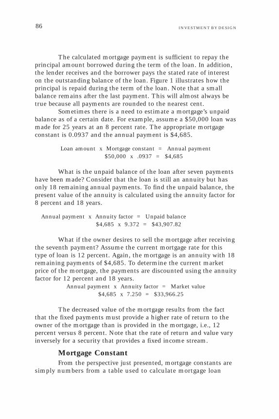
INVESTMENT BY DESIGN86
The calculated mortgage payment is sufficient to repay theprincipal amount borrowed during the term of the loan. In addition,the lender receives and the borrower pays the stated rate of intereston the outstanding balance of the loan. Figure 1 illustrates how theprincipal is repaid during the term of the loan. Note that a smallbalance remains after the last payment. This will almost always betrue because all payments are rounded to the nearest cent.
Sometimes there is a need to estimate a mortgage’s unpaidbalance as of a certain date. For example, assume a $50,000 loan wasmade for 25 years at an 8 percent rate. The appropriate mortgageconstant is 0.0937 and the annual payment is $4,685.
Loan amount x Mortgage constant = Annual payment$50,000 x .0937 = $4,685
What is the unpaid balance of the loan after seven paymentshave been made? Consider that the loan is still an annuity but hasonly 18 remaining annual payments. To find the unpaid balance, thepresent value of the annuity is calculated using the annuity factor for8 percent and 18 years.
Annual payment x Annuity factor = Unpaid balance $4,685 x 9.372 = $43,907.82
What if the owner desires to sell the mortgage after receivingthe seventh payment? Assume the current mortgage rate for thistype of loan is 12 percent. Again, the mortgage is an annuity with 18remaining payments of $4,685. To determine the current marketprice of the mortgage, the payments are discounted using the annuityfactor for 12 percent and 18 years.
Annual payment x Annuity factor = Market value $4,685 x 7.250 = $33,966.25
The decreased value of the mortgage results from the factthat the fixed payments must provide a higher rate of return to theowner of the mortgage than is provided in the mortgage, i.e., 12percent versus 8 percent. Note that the rate of return and value varyinversely for a security that provides a fixed income stream.
Mortgage ConstantFrom the perspective just presented, mortgage constants are
simply numbers from a table used to calculate mortgage loan

EVALUATING THE DATA 87
payments. Although this is true, mortgage constants also indicate thecash cost of borrowing money in much the same way as the interestrate for other types of loans. For example, on a $100,000, 12 percent,interest-only loan, the borrower expects to pay $12,000 annualinterest.
Annual interest
= Interest rate
Loan amount
$12,000 = 12 percent
$100,000
Because the mortgage loan payment includes principal andinterest, the annual payment must be larger than the amountsufficient to pay the annual interest. If a 12 percent, $100,000mortgage loan is to be repaid in 25 years, the annual payment is$12,750.
Mortgage constant x Loan amount = Loan payment .1275 x $100,000 = $12,750
Rearranging terms:
Loan payment (principal + interest) = Mortgage constant
Loan amount
$12,750 = .1275 percent
$100,000
Thus, the mortgage constant, like the interest rate, expressesthe cash cost of borrowing money. Because of this, the mortgageconstant is often quoted as an indicator of borrowing costs in amanner similar to the interest rate. When this is done, the mortgageconstant is expressed in percentage terms, not as a decimal fraction–12.75 percent, not 0.1275.
The mortgage constant at a particular interest rate alwaysexceeds that interest rate because it includes the amount neces-sary to repay the loan over the life of the loan and pay the intereston the loan. Therefore, extending the maturity of the loan reducesthe payment because the principal repayment is spread over moreyears. Thus, the mortgage constant is a function of the interest rateand the maturity. A review of a mortgage constant table reveals thatas the loan maturity is increased, the mortgage constant decreasesfrom one plus the interest rate to a value almost equal to the interestrate (the interest rate is the mathematical limit of the function).

INVESTMENT BY DESIGN88
Figure 2. Reduction in Annual Payments Requiredto Amortize a $1,000 Loan
at Selected Rates and Maturities
Interest Annual payment Decrease from Rate (%) 15 years 20 years 15-year payment (%)
6 $102.96 $ 87.19 15.328 116.83 101.85 12.82
10 131.47 117.46 10.6612 146.83 133.88 8.82
Interest Annual payment Decrease from Rate (%) 20 years 25 years 20-year payment (%)
6 $ 87.19 $ 78.23 10.278 101.85 93.68 8.02
10 117.46 110.17 6.2112 133.88 127.50 4.76
Interest Annual payment Decrease from Rate (%) 25 years 30 years 25-year payment (%)
6 $ 78.23 $ 72.65 7.138 93.68 88.83 5.18
10 110.17 106.08 3.7112 127.50 124.14 2.63
For example, mortgage payments were calculated at fourdifferent interest rates and for increasing maturities. These compari-sons are presented in Figure 2. The mortgage constant and, therefore,the annual cost of borrowing decreases as the maturity of the loanincreases. Note, however, that the percentage decrease is largestwhen the loan term is increased from 15 to 20 years and thedecrease is least when the loan term is increased from 25 to 30years. Further note that at higher interest rates there is less to begained in the way of mortgage payment reduction from extending theloan’s maturity than there is at lower interest rates.
The ready availability of calculators and computers allowsmost mortgage loan calculations to be made quickly and easily.Sometimes, however, solving a problem requires more than knowl-edge of the proper calculator keystrokes. In such cases, basic presentvalue concepts such as annuities and mortgage constants can be usedto assist in problem solving. Knowledge of these concepts providesgreater understanding of the usefulness of the result.

EVALUATING THE DATA 89
Now that the basics of present value have been presented,the use of present value techniques to estimate the value of income-producing real estate will be examined. Although some investmentconsiderations are introduced, the main focus of this series continuesto be explaining the mechanics of present value techniques.
As demonstrated in this section, the present value of all theexpected cash benefits, discounted at the appropriate discount rate isthe maximum price that can be paid for the expected cash benefits ifthe required return is to be obtained. This maximum price may becalled the property’s investment value. Investors should seekproperties with investment values in excess of their cost.
The real estate investor anticipates cash benefits in the formof after-tax cash flow from operations and resale. When debt is used,the mortgage lender generally receives periodic mortgage payments ofa predetermined amount but also may expect a share of otherbenefits such as rents, cash flow or appreciation. Thus, an incomeproducing property’s investment value is equal to the presentvalue of all cash benefits expected by the equity investor, discountedat the investor’s required rate of return, plus the cash benefitsexpected by the lender, discounted at the lender’s required rate ofreturn.
Estimating a property’s investment value is important. Thepresent value approach reflects all variables that contribute to aproperty’s investment value and that an investor considers in mak-ing the investment decision. If the property’s investment value doesnot equal or exceed its purchase price or cost to develop, the propertyshould not be considered further.
The property’s cash benefits are based on projections andassumptions about expected rental rates, vacancy rates and operatingexpenses, financing terms and loan amount, tax rates and theprojected holding period made by the equity investor and the lender.Because these projections and assumptions result in estimating theafter-tax cash flow from operations and resale (the equity investor’sbenefits) and the property’s estimated debt service (the lender’s
July 1990
Wayne E. EtterEstimating Value
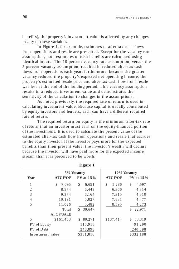
INVESTMENT BY DESIGN90
benefits), the property’s investment value is affected by any changesin any of these variables.
In Figure 1, for example, estimates of after-tax cash flowsfrom operations and resale are presented. Except for the vacancy rateassumption, both estimates of cash benefits are calculated usingidentical inputs. The 10 percent vacancy rate assumption, versus the5 percent vacancy assumption, resulted in reduced after-tax cashflows from operations each year; furthermore, because the greatervacancy reduced the property’s expected net operating income, theproperty’s estimated resale price and after-tax cash flow from resalewas less at the end of the holding period. This vacancy assumptionresults in a reduced investment value and demonstrates thesensitivity of the calculation to changes in the assumptions.
As noted previously, the required rate of return is used incalculating investment value. Because capital is usually contributedby equity investors and lenders, each can have a different requiredrate of return.
The required return on equity is the minimum after-tax rateof return that an investor must earn on the equity-financed portionof the investment. It is used to calculate the present value of theestimated after-tax cash flow from operations and resale that accruesto the equity investor. If the investor pays more for the expectedbenefits than their present value, the investor’s wealth will declinebecause the investor will have paid more for the expected incomestream than it is perceived to be worth.
Figure 1
5% Vacancy 10% VacancyYear ATCF/OP PV at 15% ATCF/OP PV at 15%
1 $ 7,695 $ 6,691 $ 5,286 $ 4,5972 8,574 6,443 6,366 4,8143 9,374 6,164 7,315 4,8104 10,191 5,827 7,831 4,4775 11,026 5,482 8,595 4,273
Total $ 30,647 $ 22,971ATCF/SALE
5 $161,453 $ 80,271 $137,414 $ 68,319PV of Equity 110,918 91,290PV of Debt 240,898 240,898Investment value $351,816 $332,188

EVALUATING THE DATA 91
The lending rate is the lender’s required rate of return, but itis not necessary to discount the lender’s expected benefits to find thepresent value of the lender’s portion: the loan amount is equal to thepresent value of the lender’s expected benefits (mortgage receipts,plus expected participation, if any) discounted at the lender’s re-quired rate of return (the lending rate). Thus, as shown in Figure 1,investment value may be calculated by adding the loan amount tothe present value of the equity benefits.
The property’s perceived risk, the terms of purchase, itsfinancing or a particular investor’s tax situation can affect theproperty’s investment value for a particular investor. Thus, oneinvestor is willing to pay more for a particular property than anotherinvestor. For example, the effect of using a 25 percent required rate ofreturn instead of 15 percent in calculating investment value is shownin Figure 2. The difference in the two investment values resultsentirely from the difference in the investor’s required rate of return,which reflects a difference in the investor’s perception of the theproperty’s risk. The degree of risk depends on the difference betweenexpected and actual outcomes. If the expected outcome is guaran-teed, then the risk is negligible; if there is great uncertainty about theexpected outcome, then the risk is significant. The usual assumptionis that riskier investment streams are discounted at higher rates.
The effect of debt financing on a property’s investment valuealso can be analyzed. For example, the effect of increasing theamount of debt from 75 percent of cost to 90 percent of cost when
Figure 2
Year ATCF/OP PV at 15% PV at 25%
1 $ 7,695 $ 6,691 $ 6,1562 8,574 6,443 5,4873 9,374 6,164 4,7994 10,191 5,827 4,1745 11,026 5,482 3,613
Total $ 30,647 $ 24,229ATCF/SALE
5 $161,453 80,271 52,905PV of Equity $110,918 $ 77,134PV of Debt 240,898 240,898Investment value $351,816 $318,032

INVESTMENT BY DESIGN92
there is positive financial leverage is presented in Figure 3. If no otherassumptions are changed, this change increases the property’sinvestment value. Such a result is entirely in accord with what isobserved in the real world: when lenders finance more generously,investors are willing to pay higher prices for property. Althoughinvestors may not make such calculations, they do understand thebenefits of using more debt. Of course, they may not always considerthe consequences of additional risk accompanying the additionaldebt.
Thus, the investment value is for a particular property andfor a particular set of circumstances. Because it is not an estimate ofmarket value, the investor cannot necessarily expect to purchase orsell the property for the estimated investment value; rather, this isthe value of the property using a particular set of assumptions; ifunreasonable assumptions are made, the investment value calculatedfor a particular investor may vary from the property’s market price.
Obviously, these factors also affect the property’s expectedinternal rate of return and net present value of equity as well. How-ever, the present value approach to estimating investment value isimportant because it is possible to determine the effect of particularassumptions on the property’s investment value, and, therefore, it ispossible to explain why particular investors are willing to pay a pricefor a property while other investors believe the property is overpriced:the assumptions used and the terms available produce a higherestimate of investment value. Negotiations between buyers and
Figure 3
75% Debt 90% DebtYear ATCF/OP PV at 15% ATCF/OP PV at 15%
1 $ 7,695 $ 6,691 $ 2,143 $ 1,8632 8,574 6,443 3,313 2,5053 9,374 6,164 4,518 2,9714 10,191 5,837 5,759 3,2935 11,026 5,482 7,038 3,499
Total $ 30,647 $ 14,131ATCF/SALE
5 $161,453 80,271 116,903 58,121PV of Equity $110,918 $ 72,252PV of Debt 240,898 289,877Investment value $351,816 $362,129

EVALUATING THE DATA 93
sellers revolve about terms and price; therefore, the calculatedinvestment value may be compared to a property’s cost or offeringprice.
Income capitalization often is used to estimate a property’scurrent or future market value. Typically for this purpose, aproperty’s net operating income (NOI) for an appropriate year isdivided by the overall capitalization rate derived from the market.Assume, for example, that a property’s estimated NOI is $10,000and an overall capitalization rate of 10 percent is used.
Net operating incomeEstimated market value =
Overall capitalization rate
$10,000 $100,000 =
.10
Income capitalization and ordinary present value calcula-tions can be combined to estimate market value. For example,assume a property’s NOI is expected to increase from $5,000 to$10,000 per year over a five-year period and then stabilize at$10,000 per year. Capitalizing the first year’s NOI produces a valueof $50,000, which undervalues the property; capitalizing the stabi-lized NOI produces a value of $100,000, which overvalues theproperty. But by adding the present value of the NOI for years onethrough five to the present value of the property’s capitalized value atthe end of year five, a better estimate of the property’s market valueis obtained. These calculations are presented in Figure 4.
Figure 4
Capitalized Present ValueYear NOI Value at 10%
1 $ 5,000 $4,545.452 6,000 4,958.683 7,000 5,259.204 8,000 5,464.115 10,000 6,209.21
10,000 = $100,000 62,092.13
.10 $88,528.79

INVESTMENT BY DESIGN94
However, what if the demand for space is currently depressedand the property’s expected increase in NOI is based on an expectedincrease in demand for space? Although the analyst may beconvinced that the demand will recover by the fifth year, the analystis concerned that the projected demand levels in the early years willnot be achieved. It may be prudent, therefore, to reflect thisperceived risk by adopting the unusual approach of discounting theNOI in the early years at a higher rate than the later years when theNOI is approaching the stabilized level (see Figure 5). A comparisonof Figures 4 and 5 indicates that the riskier income stream has thelower value.
Figure 5
Capitalized Discount Present ValueYear NOI Value Rate (%) at 10%
1 $ 5,000 12.0 $ 4,464.292 6,000 11.5 4,826.163 7,000 11.0 5,118.344 8,000 10.5 5,365.885 10,000 10.0 6,209.21
10,000 = $100,000 10.0 62,092.13
.10 $88,076.01
Appraisal reports sometimes contain calculations similar tothose in Figure 4 and 5. These should be examined closely; inparticular, the discount rate selected should be carefully explainedand justified. In some cases, the discount rate is related to returnsavailable from securities such as U.S. government bonds orcertificates of deposit rather than the property market. However,when the same income stream is being valued, the discount rateand the capitalization rate ought to be derived from the samesource.
Because of recent developments in financial calculators andpersonal computer software, it is possible to solve quickly a numberof real estate present value problems. Even with such assistance,however, it is necessary to know how present value works. Providingthis knowledge is the purpose of the last three sections.

EVALUATING THE DATA 95
Many commercial property market brokers, lenders andowners use real estate appraisals having an income approach valueestimate derived from direct capitalization and discounted cash flow(DCF) analyses. The differences between these methods and theirappropriate use are the focus of this section.
To estimate value with direct capitalization, a property’sstabilized net operating income (NOI) is divided by the marketcapitalization rate (Figure 1). Estimating value with DCF analysisrequires estimates of each year’s NOI along with the property’sexpected reversion value at the end of the analysis period. Usuallythe analyst uses income capitalization to estimate the reversion.These expected cash benefits are then discounted at the appropriaterate to obtain the market value estimate, also shown in Figure 1.
Estimating Net Operating IncomeAlthough these calculations are simple and straightforward,
they depend on the appraiser’s assumptions or estimates. Whenusing direct capitalization, the property’s stabilized NOI must beestimated. This estimate is developed from market data (rentalrates, vacancy and collection loss rates and operating expense data)for comparable properties in the market area; it represents theappraiser’s opinion of how the property ought to perform.
Because the appraiser’s opinion is based on observed marketdata, it’s difficult to quibble with his or her NOI estimate. When amarket is “normal,” the notion of stabilized NOI is particularlyuseful.
But two areas are of special concern. First, what if theproperty has significant vacancy at the time of the appraisal? Obvi-ously, no one develops a property with the expectation of significant,permanent vacancy. So, the appraiser may use a market vacancy rate(or the anticipated vacancy rate when the property is fully leased)
Direct Capitalizationor Discounted CashFlow Analysis?
Fall 1994
Wayne E. Etter

INVESTMENT BY DESIGN96
Figure 1. Estimating Value with Direct Capitalizationand DCF Analysis
NOI $10,000Value = ————————— = ––—— = $100,000
Capitalization rate .10
Year NOI Reversion Total1 $10,000 $10,0002 10,000 10,0003 10,000 10,0004 10,000 10,0005 10,000 $100,000 $110,000
Present value at 10% = $100,000
rather than the property’s actual vacancy rate. This results in alarger NOI for the subject property and may overstate the property’svalue. Second, if the property’s future NOI is expected to increasebecause of greater demand for space that leads to higher rental rates,direct capitalization of a single year’s NOI may understate theproperty’s value.
Because DCF analysis permits annual adjustments in rentalrates, vacancy and collection loss rates and operating expenses, DCFanalysis can be used to reflect a buyer’s expectations of increasingNOI over time. When a property is expected to become fully leasedduring the next three to five years, for example, the current vacancyrate can be reduced until the desired occupancy is reached.
This specification of expected changes results in realisticNOI estimates throughout the period–a result far superior to capital-izing a single year’s NOI. On the other hand, just assuming that thevacancy rate will be reduced during the three-year period may lead tooverestimating NOI.
DCF analysis is ideally suited for situations such as this.However, DCF analysis does not add much useful information whenthe subject property is fully leased and no changes in occupancy orthe external environment are anticipated that will affect NOI. Asshown in Figure 1, the present value of a series of equal annual cashflows is equivalent to the capitalized value.

EVALUATING THE DATA 97
It is not an error to use DCF analysis to value a propertywhen no significant change in NOI is expected. However, appraisalreport users should understand that this technique’s results are nobetter than those produced by a correct application of direct capitali-zation. Of course, if both techniques, properly used, achieve similarvalues, the estimated value has greater credibility.
Selecting Capitalization and Discount RatesTheoretically, concerns about capitalizing a single year’s NOI
are eliminated by the appraiser’s skill in deriving the market capitali-zation rate from comparable sales. If the market capitalization rate isderived from sales of properties with vacancy rates comparable to thesubject and with comparable buyer expectations about becomingfully leased (or for increased NOI), the subject property’s value couldbe estimated with an unadjusted NOI and the market capitalizationrate.
Buyers who expect their properties’ occupancy levels toimprove pay prices that reflect this expectation. Likewise, buyerswho expect the future NOI of their properties to increase pay pricesreflecting that expectation. In both cases, expectations are reflectedby observed capitalization rates.
The appraiser’s problem arises when appropriatecomparables cannot be located. In this case, the appraiser mustdevelop the capitalization rate and estimate the NOI from the bestavailable comparables to produce a market value estimate thatreflects these expectations.
For DCF analysis, an appropriate discount rate is used toconvert the NOI estimates to a value estimate. When DCF analysisis used to estimate a property’s market value, the discount rateought to be extracted from the market using the data of comparableproperties. Thus, the need for appropriate comparables is the samefor DCF analysis and for direct capitalization. (When DCF analysisis used for investment analysis, the investor’s required rate of returnought to be used to discount the expected cash flow.)
Deriving a discount rate from the market is more difficultthan estimating the market capitalization rate. For each comparableproperty used in the derivation, the buyer’s expectations about futureNOI and reversion would have to be determined. This would allowcalculation of the discount rate that equates these expectations to thepurchase price. (Estimating the market capitalization rate requiresonly each comparable property’s NOI and the reported sales price.)

INVESTMENT BY DESIGN98
After obtaining the discount rate for each comparable prop-erty, the analyst would select the appropriate discount rate for thesubject property. The process is the same as choosing the appropriatecapitalization rate from comparable sales.
While this procedure is possible, it would be difficult inpractice. Therefore, the discount rate often is estimated by adding arisk premium and a liquidity premium to a relatively risk-free rate ofreturn, such as the U.S. Treasury bill rate or to the yield of someother security. This built-up rate is used to discount the expectedcash flows. Although a theoretically correct approach, its use re-quires a serious attempt to ascertain the risk and return differencesbetween the subject property and the security.
Investor surveys offer another approach for selecting anappropriate discount rate. Such surveys report investors’ expecta-tions for several different property types. The obvious problem withtheir use is that they report general expectations rather than theexpectations for a specific property in a specific market.
Sometimes several different discount rates are tried; the ratethat results in a market value estimate approximately the same asthat obtained with direct capitalization is selected. Then, thereasonableness of this rate of return is verified by comparing it toinvestor returns in other markets.
Figure 2. A Comparison of Direct Capitalizationand DCF Analysis with Income Growth
Year NOI Reversion Total1 $10,000 $10,0002 10,500 10,5003 11,000 11,0004 11,500 11,5005 12,000 $125,000 $137,000
Present value at 14.6% = $100,000
NOI $10,000Value = ————————— = ——— = $100,000 Capitalization rate .10

EVALUATING THE DATA 99
Normally, the discount rate is greater than the capitalizationrate. Why? As reported in Figure 1, if no change in cash flows isanticipated, the discount rate is equal to the capitalization rate.However, as Figure 2 shows, an increasing income stream requiresthat the discount rate be greater than the capitalization rate if thetwo separately determined values are to be equal. (They must beequal because the property can not have two values.) Therefore,because forecasts of increasing income are common, the discountrate used is normally greater than the discount rate. In fact, in aperfect world, the discount rate is equal to the capitalization rate plusthe weighted average of the net operating income and the propertyvalue annual growth rates.
Choice Difficult, NecessaryDirect capitalization and DCF analysis are each appropriate
in certain circumstances. In particular, direct capitalization is wellsuited for properties expected to have stable NOI; DCF analysis iswell suited for properties expected to have fluctuating NOI. Selectingthe appropriate capitalization rate and discount rate may sometimesbe difficult for both techniques.
A prime benefit of DCF analysis is that in gathering the datarequired to estimate NOI for the analysis period, a good deal islearned about the subject property’s prospects. A DCF analysisrequires careful consideration of expected supply and demand for aparticular type of space and operating expenses. Properly done, suchan analysis can provide much information not apparent throughdirect capitalization.
Often, however, the primary use of DCF analysis is theconfirmation of the direct capitalization market value estimate.Despite the fact that for some properties the NOI estimates used inDCF analysis may be more accurate, independent confirmation ofthe direct capitalization market value estimate requires an appropri-ate discount rate. Merely using a discount rate that seems reason-able to get a value estimate with DCF analysis approximately equalto the value estimate obtained with direct capitalization is not aconfirmation.

INVESTMENT BY DESIGN100
Debt Financing:Rewards and RisksUsing debt to finance income-producing real estate is an
accepted practice. Although the rewards of debt financing can besignificant, so are the risks. Unfortunately, many investors anticipateonly the rewards of debt financing and give little attention to risks.
Obviously, when debt financing is arranged, both the lenderand the investor anticipate that income will be adequate to servicethe debt; in fact, the usual assumption is that a property’s netoperating income will increase during theholding period. With fixed debt service,this assumption results in an improvingmargin of safety during the holdingperiod (Figure 1).
Nevertheless, the use of debtgives rise to financial risk–the risk thatthere will be inadequate income to meetdebt service requirements. Althoughthere may be a trend toward the use ofless debt in some real estate syndications,the possible benefit of using less debt is
October 1989
Wayne E. Etter
Analyzing Riskand the Use of Debt
9

ANALYZING RISK AND THE USE OF DEBT 101
not well understood. In today’s market, however, considerationshould be given to revising the accepted practice of using as muchdebt as can be obtained to finance real estate. This could create anew investment product with reduced risk that appeals to investorswary of traditionally financed real estate.
Why Use Debt?The expected after-tax rate of return from a real estate
investment is determined by the expected benefits of the invest-ment–after-tax cash flow and appreciation–and the cash required topurchase the property. Investors determine a proposed real estateinvestment’s expected rate of return and compare the result with theminimum return required to undertake the investment. A furthertest is a comparison of the property’s estimated investment valuewith its cost. A property’s investment value is equal to the presentvalue of all the cash benefits expected by the equity investor, dis-counted at the investor’s required rate of return, plus the amount ofthe mortgage.
Real estate investors wish to use debt if its use will increasethe after-tax return on equity (ATRE) and the property’s investmentvalue. Using debt this way is known as financial leverage. For in-stance, the ATRE and the investment value were calculated for atypically structured income property using varying amounts of debtwith the following results:
Amount of debt (%) ATRE (%) Investment value ($)
None 13.26 301,198 50 17.23 334,943 75 23.84 351,815 90 37.27 361,329
When the amount of debt is held constant at 75 percent andthe interest rate is varied, the following results are obtained:
Interest rate (%) ATRE (%) Investment value ($)
10 27.04 362,97412 23.84 351,81514 20.42 340,10616 16.77 327,50618 13.26 314,82920 9.90 302,103

INVESTMENT BY DESIGN102
Analyzing these results reveals that the ATRE and theinvestment value of the property increase as a larger proportion ofthe property is financed with debt having a constant cost. Also theATRE and the investment value decrease as the interest rate isincreased when the proportion of financing is held constant. Eventu-ally, the ATRE and the investment value, when financed with high-cost debt, are less than the property’s ATRE and the investmentvalue without debt. Thus, the beneficial effects of debt financing arelimited–expensive debt is worse than no debt.
Other factors also affect whether or not the use of debt isfavorable. If the expected benefits (after-tax cash flow and apprecia-tion) increase for reasons such as increased rent levels, reducedvacancy rates or operating expenses, increased rate of appreciation orreduced tax rates, the expected ATRE and the investment value willincrease at any given debt level or interest rate. Therefore, increasedinvestor expectations justify the use of higher cost debt. Duringperiods of rapid property appreciation, high interest rates will notdeter investors from using debt financing to buy properties.
An investor is indifferent between two investment opportuni-ties having the same expected rate of return only if they have thesame risk. Thus, the returns of various investments often are com-pared by evaluating both their risk and their expected return. Theusual assumption is that riskier investments have increased returns(Figure 2). Such investments also can have increased losses; theline represents expected returns.
Risk exists in all projects, but some are more risky thanothers. The degree of risk depends on the difference between ex-pected and actual outcomes. If the expected outcome is guaranteed,then the risk is negligible; if there is great uncertainty about theexpected outcome, then the risk is significant.
As earlier stated, financial risk ispresent when debt is used. Because theinvestor and the lender believe that thedebt can be managed when the property isfinanced, the principal source of financialrisk is unanticipated variation in theproperty’s income stream over time.There is a particularly important connec-tion between business risk (the risk offailing to generate sufficient income),management risk (the risk of failing torespond properly to changes in the

ANALYZING RISK AND THE USE OF DEBT 103
business environment and, therefore, failing to earn a satisfactoryreturn) and financial risk (the risk of having inadequate income tomeet debt service requirements).
If a project is believed to have little business and manage-ment risk, then a high proportion of potential gross income could becommitted to the payment of operating expenses and debt service. Ifthe opposite is true, a much lower proportion of potential grossincome should be committed to the payment of operating expensesand debt service. A project’s operating expenses are somewhat fixedin the short-run and vary directly with potential gross income overtime; the operating expense ratio should be constant over time.Limiting the total funds available for the payment of operatingexpenses and debt service has a direct impact on the amount offunds available for debt service and, therefore, the amount of debt,called allowable debt.
Projects believed to have little business and management risk(i.e., there is little expected variation in the income stream) couldhave higher levels of debt without creating excessive financial risk.On the other hand, projects believed to have significant exposure tobusiness and management risk should have much less debt so thatexcessive financial risk is not created. For example, assume twoproperties are identical except for risk:
Low-risk High-riskproperty property
Potential gross income $100,000 $100,000Percentage allowed for operating expenses and debt service .90 .60Funds available for operating expenses and debt service $90,000 $60,000Operating expenses 30,000 30,000Available for debt service $60,000 $30,000Divide by mortgage constant .1275 .1275Allowable debt $470,588 $235,294
At any given mortgage constant, $60,000 will service twiceas much debt as $30,000. This approach allows the risky buildingmuch less debt financing and achieves a result similar to what isobserved in other types of enterprises. Risky businesses must borrowless than safer ventures.

INVESTMENT BY DESIGN104
What Are the Benefits of This Approach?The foregoing approach to risk results in some properties
being financed with much less debt than is considered normal. But,for either building, the use of more debt to increase the expectedATRE or investment value increases the likelihood of default.
Suppose, therefore, that a property is financed with morethan the amount of allowable debt to raise its expected ATRE andinvestment value. This will cause total risk to exceed an acceptablelevel given the investors’ required return. Under such a circum-stance, investors should increase their required rate of return. Theadditional return expected from the additional debt is not withoutadditional risk–greater risk must be matched by a greater requiredreturn–and, therefore, the calculated increase in the ATRE is not anadditional benefit received without cost. Likewise, when estimating aproperty’s investment value, investors must apply a higher discountrate to the expected benefit stream. As a result, the beneficial effectof using more debt may be offset by the effect of the higher discountrate with the possible result of a decrease in the property’s invest-ment value.
On the other hand, it is possible to use even less debt or nodebt to further reduce the exposure to financial risk and, thereby,reduce total risk. Using less debt (or no debt) should increase theinvestment quality of a property; such a course of action shouldresult in investors reducing their required rate of return for theproperty and applying a lower discount rate when calculating invest-ment value. As a result, the reduced benefits from using less debtmay be offset by the willingness of investors to accept a lower ATREand by the effect of the lower discount rate with the possible result ofan increase in the property’s investment value.
Assume, for instance, that a commercial property is leased toquality tenants; the lease has several years to run and there is reasonto believe the current tenants will wish to renew their lease. Theproperty may be classified as a low-risk property because there is areasonable probability that the difference between the property’sexpected income stream and actual income stream will be small. Ifthe property is conservatively financed (perhaps even 100 percentequity), it will be even more attractive to conservative investors.Under such circumstances, the property’s income stream will behighly predictable; investors will pay a premium price for such aproperty.

ANALYZING RISK AND THE USE OF DEBT 105
Next consider a property characterized by more business andfinancial risk–fewer quality tenants with less assurance of leaserenewal when the current leases expire. There is a greater probabilitythat there will be a difference between the expected income streamand the actual income stream. Financing such a property with, say,75 percent debt may result in the property’s total risk being exces-sive. But, if this property is financed with less than 75 percent debt(again, perhaps even 100 percent equity), investors may view theproperty as an attractive investment. Properly estimated, theproperty’s investment value may be higher with less or no debt.
Thus, the question is: Can an investor’s lower required rateof return or discount rate offset the beneficial effects of financialleverage on a property’s expected rate of return and investmentvalue? If so, income-producing real estate could be transferred fromthe high-risk investment category when it is financed with a largeproportion of debt to a much lower risk category. Only by relatinginvestors’ required returns with risk and by calculating the invest-ment value of a property using various assumptions can this ques-tion be answered. If the answer is positive, more investors might beattracted to real estate because income-producing real estate canbecome a much less risky investment.
The real estate appraisal process depends on sales of compa-rable properties and other market data. Although adjustments can bemade when the sold properties are not perfectly comparable to thesubject property, some sales are required. However, there have beenfew recent property sales in some markets, and bid and ask pricemay differ considerably.
Today, therefore, real estate appraisers often work in marketswhere sales of comparable properties are infrequent or nonexistent.To value properties in such a difficult market, they must use tech-niques to compensate for the lacking market data.
This article examines the effect of few comparable sales onone aspect of the appraisal process.
Appraising inDifficult Markets
January 1992
Wayne E. Etter

INVESTMENT BY DESIGN106
Approaches to Real Estate AppraisalThere are three commonly accepted approaches to estimat-
ing value: the sales comparison approach, the cost approach and theincome approach. Each is dependent on accurate market data. But ina market characterized by few sales and little development activity,certain data are difficult to obtain.
• Sales comparison approach. The estimate of market value isbased on recent sales of comparable properties. A lack of recentcomparable sales reduces this approach’s contribution to thefinal estimate of value.
• Cost approach. The estimate of market value is based on thecost of developing a similar property. When market values areless than the cost of developing a new property, little, if any,development takes place and the cost approach’s contribution tothe final estimate of value is limited.
• Income approach. The estimate of market value is based onthe relationship between the income and value of similarproperties. A lack of recent sales of comparable propertiesmakes it difficult to estimate the relationship between incomeand value. When sufficient recent sales are not available,appraisers sometimes use other methods, such as the band ofinvestment approach, to estimate the relationship.
Because the sales comparison approach obviously cannot beused when there are few, if any, recent sales of comparable propertiesand because the cost approach explains little when the cost ofdevelopment exceeds the market value, appraisers rely on the incomeapproach in such markets.
Income Capitalization ApproachTo estimate a property’s market value by the income capitali-
zation approach, the property’s stabilized net operating income(NOI) is divided by the appropriate overall capitalization rate (OAR).
NOI is a proxy for the investor’s expected benefits–the after-tax cash flow from operations and resale (NOI ignores debt and taximplications). NOI is estimated by using market rents and vacancyrates, typical operating expenses and so forth. The OAR is estimatedfrom comparable properties–comparable properties’ NOI is dividedby their reported sales price and the OAR is obtained. Thus, theresulting value is estimated from market data; if the data are gath-ered from actual comparables, the resulting value estimate is reliable.
The price paid by an investor for the expected benefitsreflects the investor’s required return. The OAR is not a real rate of

ANALYZING RISK AND THE USE OF DEBT 107
return; rather, it reflects the relationship between a proxy for theexpected benefits and the price paid for those benefits. As the per-ceived risk of receiving the benefits is reduced, the investor will pay agreater price for the benefits (and vice versa).
Appraisers also use the band of investment approach toestimate the OAR. This approach recognizes that income-producingreal estate typically is financed with a mixture of debt and equity andthat each financing source must receive a satisfactory return. If thereare no recent comparable sales, the OAR cannot be derived frommarket data, but the band of investment approach can be used toestimate the OAR if financing is available on the assumed terms.
When using the band of investment approach, the OAR isestimated by taking a weighted average of the lender’s requiredreturn (the mortgage constant) and the investor’s required equitycapitalization rate (before-tax cash flow divided by the initial equityinvestment).
In theory, the OAR estimated by the band of investmentapproach is equal to the OAR estimated from comparable salesbecause both approaches should yield the same value. Thus:
NOI=
NOI= Value
OAR1 OAR2
OAR1 = market data approachOAR2 = band of investment approach
The method used to estimate the OAR does not matter ifthe assumed financing terms are available. But, what if the OAR isestimated by the band of investment approach and the assumedfinancing terms are not actually available in the market? This is animportant question. Although many income properties cannot befinanced today, many appraisers continue to assume the availabil-ity of typical financing when they estimate the value of suchproperties. To answer this question, the role of financial leveragemust be considered.
The purpose of financial leverage is to enhance the investor ’safter-tax return on equity. If there is less debt (or no debt), the after-tax return on equity is reduced, holding all other variables constant.Of course, using less debt reduces the project’s financial risk and aninvestor might reduce the required rate of return because of theproject’s reduced financial risk. (For a more complete discussion offinancial leverage, see “Debt Financing: Rewards and Risks.”)

INVESTMENT BY DESIGN108
However, using less debt than has been typical (especially ifthe typical debt is nonrecourse debt), may be viewed as an increasedrisk by the investor who must now contribute a larger percentage ofequity than before. The investor may require a larger return onequity, even though the project’s financial risk is reduced. At the veryleast, the advantage of financial leverage is lost and the investor mayoffer less for the property to earn the same after-tax return when theproperty is acquired with reduced debt or no debt.
Consider, for example, an income property producing a$39,000 NOI. Assuming that it can be financed with 75 percent debthaving a 12.75 percent mortgage constant and that the equityinvestor’s required capitalization rate is 10.3 percent, the estimatedOAR is 12.1 percent and the property’s estimated value is $322,314.
Proportion x CostDebt .75 .1275 = .096Equity .25 .1030 = .026OAR .121*
NOI $39,000Value = = $322,314
OAR .121
(* difference due to rounding)
Further assume that an investor uses a discounted cash flowmodel with specific assumptions about rent, vacancy rates, operatingexpenses, holding period, resale price and so forth to calculate theexpected after-tax internal rate of return on equity (ATIRRE). If theinvestor uses these assumptions along with a $322,314 purchaseprice and the foregoing financing terms, the expected ATIRRE isapproximately 24 percent. If the investor discovers that lenders willlend only 60 percent of the purchase price, what is the OAR and theproperty’s estimated value? If the debt and equity proportions arechanged, the following result is obtained.
Proportion x Cost
Debt .60 .1275 = .077Equity .40 .1030 = .041OAR .118
NOI $39,000Value = = = $329,950
OAR .118

ANALYZING RISK AND THE USE OF DEBT 109
This, however, is an error. The property’s value actually willdecrease (rather than increase from $322,314 to $329,950) be-cause of the reduced financing. Why? If the investor requires anATIRRE of approximately 24 percent to undertake the investment,the purchase price must decrease, holding constant all factors exceptfinancing. Using the same assumptions as before, an ATIRRE ofabout 24 percent results when the investor pays $289,000 andobtains a loan equal to 60 percent of the purchase price using amortgage constant of 0.1275. Thus, the property’s capitalization rateis 13.5 percent instead of 11.8 percent; this implies a required equitycapitalization rate of 14.5 percent.
NOI $39,000 = OAR = = .135
Value 289,000
Proportion x CostDebt .60 .1275 = .077Equity .40 .1450 = .058OAR .135
What if financing is unavailable? If the investor’s requiredATIRRE remains the same, the price must decrease to approximately$208,600. Holding all other factors constant, the property’s capitali-zation rate and equity capitalization rate increase to 18.7 percent.
NOI $39,000= OAR = = .187
Value 208,600
Proportion x CostDebt n.a. nil = nilEquity 1.00 .1870 = .187OAR .187
Relationship to Current MarketHow do these calculations relate to the current market?
They help to explain the gap between the sellers’ expected price andthe price buyers are willing to pay. Potential buyers are noting boththe reduced expectations about rental income and the lack oftypical financing. In the absence of market transactions, manyappraisal reports rely on the band of investment approach (or one ofthe similar approaches) to derive an OAR. However, to assumefinancing terms that are not available overstates the property’sestimated market value, even though the property’s NOI may beappropriately stabilized.

INVESTMENT BY DESIGN110
Towards EvaluatingCommercialPropertiesMany lenders no longer actively pursue commercial real
estate loans. Because of the widespread delinquencies of commercialreal estate loans made in the 1980s, lenders apparently believe othersectors offer fewer problems, more opportunities or both. Addition-ally, bank risk-based capital regulations and proposed insurancecompany regulations require significantly more capital for commer-cial real estate loans than for some other types of loans and assets.
The amount of capital required is based on the risk class ofthe particular loan or asset. For example, investments in U.S.government securities are considered risk-less; commercial realestate loans are in the most risky category. A bank with assetsconcentrated in commercial real estate loans (or other assetsconsidered equally risky) needs more capital than if it invests in lessrisky assets or loans. Because capital has a cost, many commercialbanks find that investing in U.S. government securities is moreprofitable than extending commercial real estate loans. With similarrules set to take effect in the life insurance industry, that industry’srole as a supplier of commercial real estate loans may diminish.
Among lenders who consider making new commercial realestate loans, many are unwilling to make them on a nonrecoursebasis; they require personal guarantees in addition to liens on theproperty. While other sources of commercial real estate financing,such as real estate investment trusts, are increasingly important, theissue of evaluating project risk appears to be central to the currentproblems of financing commercial real estate.
Almost everyone who considers the problem of analyzingcommercial real estate suggests increasing the discount rate as ameans of compensating for risk. Increasing the discount rate reducesthe present value of the estimated cash flows and, therefore, theproperty’s value because it is risky. Although this approach is correct,this section focuses on controlling risk rather than adjusting for
Spring 1994
Wayne E. Etter

ANALYZING RISK AND THE USE OF DEBT 111
risk. Paying a smaller price for risky real estate does not eliminatethe risk–the buyer just loses less.
Although several risks affect real estate value, three risks–financial, business and management–are discussed here. Financialrisk (the possibility of inadequate income to service debt) is presentwhen debt is used. The investor and the lender must be convincedthat the debt can be managed if the pro forma projections madewhen the property is financed are achieved. The principal reasonswhy the debt service requirements may not be met are business risk(the property may fail to generate sufficient income) and manage-ment risk (the property’s managers may fail to respond properly tochanges in the business environment and, therefore, fail to earn asatisfactory return).
A property’s income stream is the principal determinant ofits value and the source of the loan’s repayment unless the loan isotherwise secured. Thus, if the property’s income stream varies overtime, there is great potential for default if the loan amount is deter-mined, for example, by assuming a 95 percent occupancy rate andlending 75 percent of a property’s capitalized value.
If the degree of business and management risk is assessedand variation in the property’s income stream over time is highlyprobable, less debt should be used.
Rating properties according to the expected stability of theincome stream permits lenders to loan an appropriate amount forspecific properties so total risk is not excessive. Although this wouldbe a new approach to financing real estate, it is similar to the ap-proach used in home mortgage lending.
A prospective homebuyer cannot get a large loan just becausean expensive home is being purchased. This is true even though theloan amount normally is limited to a percentage of the home’s value;this allows the lender to foreclose on the asset in the event of adefault and sell it for an amount equal to or greater than the unpaidloan balance. However, foreclosure and sale are the lender’s lastresort; lenders prefer to have the loan repaid as agreed.
To help ensure this result, lenders qualify the prospectiveborrower’s ability to repay the loan by considering the applicant’scurrent income and financial situation, credit history and employ-ment record. If the applicant has an erratic income or employmenthistory or if an excessive proportion of the applicant’s currentmonthly income is required to service the requested loan, the lenderrefuses to grant the loan. Evaluating the stability of a commercial

INVESTMENT BY DESIGN112
property’s expected income stream is an entirely analogous analyticalproblem.
As in home mortgage lending, the beginning point inassessing the riskiness of a commercial property’s income stream isdeveloping a list of factors contributing to income stream fluctations.The factors must be developed separately for each property type(multifamily residential, office, retail, industrial). Furthermore, themajor property types must be subdivided into groups of properties ofvarying size. Other property categories are possible. The importantpoint is to compare only like properties within the relevant marketarea.
What factors are included? The following suggestions are astarter list; they are not all-inclusive.
• Economic differences among market areas are important.• Supply and demand conditions in the property’s market area
must be evaluated. Determine if an unmet need can be satis-fied. How much vacant space exists currently in the market?How likely is new space to enter the market? What is theattitude of local planning authorities toward new space?
• The competitive position of the property must be assessed.Evaluate the property’s site, age, size, construction quality anddesign relative to similar properties.
• The property’s performance must be assessed. Analyzeoccupancy, tenants’ credit quality, type of lease, average leaserates and length of lease. When appropriate, tenant mix must beevaluated.
• Additional factors must be considered for to-be-developedproperties. These include the developer’s reputation andexperience and the amount of pre-leasing. However, to-be-developed properties should be scrutinized more than seasonedproperties because they have no market or operating history.Many properties developed in the 1980s never achieved theirpro forma projections; perhaps to-be-developed propertiesshould be financed with more equity than seasoned propertiesuntil their pro forma projections are achieved.
Identifying these factors is an ideal project for organizationsof real estate professionals. Once general agreement is reached aboutwhich factors should be included and their relative importance, arating scale could be constructed.
Rating a property forces the analyst to consider carefully eachproperty characteristic in relation to other comparable properties in

ANALYZING RISK AND THE USE OF DEBT 113
the market area. For example, “Retail Center A” with several “momand pop” tenants on month-to-month leases has a much less predict-able income stream than “Retail Center B” with national credittenants on income long-term leases. Thus, Retail Center A receives alower score because it has more business and management risk. Forthe more subjective factors, scaling may be difficult.
A property’s total score varies inversely with business andmanagement risk; a low score indicates more business and manage-ment risk. When this is the case, the amount of debt financing shouldbe limited because the addition of financial risk creates excessive totalrisk. For example, assume two properties are identical except for risk:
High-risk Low-riskproperty property
Potential gross income $100,000 $100,000Percentage allowed for oper- ating expenses and debt service x .60 x .90
Funds available for operating expenses and debt service $60,000 $90,000Operating expenses - 30,000 - 30,000
Available for debt service $30,000 $60,000
Divide by mortgage constant .1275 .1275
Allowable debt $235,294 $470,588
At any given mortgage constant, $60,000 will service twiceas much debt as $30,000. This approach allows the risky buildingmuch less debt financing and achieves a result similar to what isobserved in other enterprises. Risky businesses qualify for less debtthan safer ventures.
Should an acceptable means of rating projects be developed,the regulators might reduce the amount of capital required whenlenders grant an appropriate amount of credit to finance commercialreal estate. And even when debt financing is not used, an analysis ofa property’s business and management risk is useful. A properassessment of such risk assists in the assembly of all-equity portfo-lios with a given risk level.
Finally, a project risk rating scale recognized by the marketwould increase real estate’s liquidity. Illiquidity is a major real estaterisk; if illiquidity can be reduced, there is a positive impact on realestate values.

INVESTMENT BY DESIGN114
10Asset Management
Asset ManagementEssentials
For the past several years, asset management has been muchdiscussed in real estate circles. Generally, this term describes adecision-making technique for choosing a strategy to maximize thevalue of an income-producing property.
This process is applied to a broad range of problems such asanalyzing the impact on value of a proposed property refurbishmentor considering the impact on value of gaining or losing a specifictenant. Often competing strategies are under consideration, but theone that maximizes the property’s value should be chosen.
Maximizing value is the goal of financial managers in manyindustries outside real estate. For example, when financial managersmake plant expansion or product-line decisions, they often usediscounted cash flow analysis–a technique that helps select thecourse of action giving the maximum present value.
Discounted cash flow analysis techniques have been adoptedby asset managers in the real estate industry for two basic reasons.First, these techniques are made easy by powerful financial calcula-tors and personal computers. Second, and much more important,
April 1993
Wayne E. Etter

ASSET MANAGEMENT 115
until recently, real property values appeared to increase withoutmanagement; the goal was to finance and build. Management of thecompleted asset did not appear necessary.
Eventually, the degree of overbuilding and its effects becameobvious. Today, properties require management because an annualincrease in value can no longer be taken for granted. With excessleasable space, competing successfully for tenants has become animportant goal of asset managers attempting to maintain or increaseproperty values. With this competition, the asset manager mustmake a number of decisions that could affect the property’s value.For example, how will refurbishing a property affect the occupancyrate? Or, how will increasing or decreasing the rental rate affectoccupancy? These actions affect the income stream and, in turn, thevalue of the property.
Analyzing the impact on value of such changes requiresaccurate estimates of their impact on the future income stream.When the effects are properly specified, discounted cash flow analysiscan be used to calculate whether the estimated change in the incomestream will have a positive or a negative effect on the property’svalue. Thus, there are two stages in the asset management process:developing an asset management plan to generate the data necessaryfor the analysis and analyzing the plan’s impact on the property’s value.
Developing the Asset Management PlanDeveloping the asset management plan is the most impor-
tant part of the analysis because it is the basis for selecting the beststrategy. The plan enables the asset manager to quantify the differ-ences between competing proposals and/or the status quo. The planmust be developed in detail for each alternative strategy underconsideration and should include the following points.
First, the asset manager must have a comprehensive marketstudy for the property. The market study should provide informationabout the types of space available in the market, the amount of spaceavailable, the type of space being demanded, the changes expected inthe supply and demand for space and any currently unmet marketneeds. Finally, the market study should provide an estimate of theprice prospective tenants (or buyers) are willing to pay for the space.
Second, a pro forma operating budget must be developed foreach alternative strategy being considered. The market studyprovides information about the number of square feet to be leasedand the likely rental rate. Other data to be forecast for the holdingperiod include the expected operating expenses and the marketing
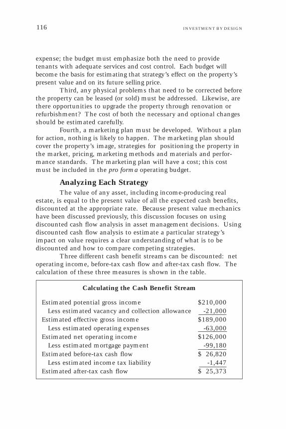
INVESTMENT BY DESIGN116
expense; the budget must emphasize both the need to providetenants with adequate services and cost control. Each budget willbecome the basis for estimating that strategy’s effect on the property’spresent value and on its future selling price.
Third, any physical problems that need to be corrected beforethe property can be leased (or sold) must be addressed. Likewise, arethere opportunities to upgrade the property through renovation orrefurbishment? The cost of both the necessary and optional changesshould be estimated carefully.
Fourth, a marketing plan must be developed. Without a planfor action, nothing is likely to happen. The marketing plan shouldcover the property’s image, strategies for positioning the property inthe market, pricing, marketing methods and materials and perfor-mance standards. The marketing plan will have a cost; this costmust be included in the pro forma operating budget.
Analyzing Each StrategyThe value of any asset, including income-producing real
estate, is equal to the present value of all the expected cash benefits,discounted at the appropriate rate. Because present value mechanicshave been discussed previously, this discussion focuses on usingdiscounted cash flow analysis in asset management decisions. Usingdiscounted cash flow analysis to estimate a particular strategy’simpact on value requires a clear understanding of what is to bediscounted and how to compare competing strategies.
Three different cash benefit streams can be discounted: netoperating income, before-tax cash flow and after-tax cash flow. Thecalculation of these three measures is shown in the table.
Calculating the Cash Benefit Stream
Estimated potential gross income $210,000 Less estimated vacancy and collection allowance -21,000Estimated effective gross income $189,000 Less estimated operating expenses -63,000Estimated net operating income $126,000 Less estimated mortgage payment -99,180Estimated before-tax cash flow $ 26,820 Less estimated income tax liability -1,447Estimated after-tax cash flow $ 25,373

ASSET MANAGEMENT 117
When the net operating income is used to estimate the valueresulting from a particular strategy, no consideration is being given tofinancing or taxes. Thus, the before-tax cash flow or after-tax cashflow should be used when the asset manager’s decision involveschoosing among financing alternatives or analyzing tax impacts.
Because mutually exclusive strategies to maximize theproperty’s value are being considered, the strategy producing thelargest net present value is chosen. Net present value is equal to thepresent value of the expected income stream plus the present valueof the property’s estimated value at the end of the analysis periodminus the strategy’s cost. This result is compared with the netpresent value of the property if no change is made.
When before-tax cash flow or after-tax cash flow fromoperations and resale is chosen as the benefit stream to discount,only the value of the equity interest is estimated; to estimate theproperty’s value, therefore, the mortgage financing amount must beadded to the present value of the equity. To compare competingstrategies, each strategy’s cost must be subtracted from theproperty’s estimated value. As before, the final value is comparedwith the property’s value if no change is made.
The appropriate discount rate must be applied to the benefitstream selected. In general, the following relationships should beused as a guide in choosing the appropriate discount rate.
Cash benefit stream Appropriate discount rateNet operating income Capitalization rateBefore-tax cash flow Before-tax, cash-on-cash return
After-tax cash flow After-tax return on equity
Sometimes the discount rate is estimated by examiningreturns available from securities such as U.S. government bonds,certificates of deposit or corporate bonds. Although such compari-sons are interesting from a risk-return standpoint, the appropriatediscount rate should be obtained from the property market.
Once the detailed elements of the plan are developed, dis-counted cash flow analysis may be used to choose the optimalstrategy. Today, however, discounted cash flow analysis is not as wellregarded as it once was.
For example, Cushman and Wakefield reports that “manyinvestors seem to have lost faith in cash flow forecasts and reportplacing more emphasis on direct capitalization of current (as opposedto forecasted) net operating income.” However, the poor investmentdecisions of the past decade based on discounted cash flow analysis

INVESTMENT BY DESIGN118
Renovating an income-producing property is an ideal applica-tion of asset management techniques. The first step in usingthese techniques is the development of an asset management plan.
The plan should include a market study, a careful determina-tion of the plan’s cost and an analysis of the renovation’s impact onthe income stream and the property’s value. Then, using the datadeveloped in the asset management plan, the decision maker mustdetermine if the renovation is justified by the increase in theproperty’s value. This article demonstrates the application of assetmanagement techniques to the proposed renovation of St. RegisPlace, a Houston mixed-use complex.
The property, located in the Galleria-River Oaks area is a242,909-square-foot, 325-unit apartment complex. In addition, a54,975-square-foot office-retail development is on the site. Thecomplex was constructed in 1954 and needed substantial repairwhen renovation was proposed in 1990.
The April 1990 monthly operating statement was typical ofthe property’s performance prior to renovation.
Rental income Apartments $108,982 Office-retail 26,182 Total $135,164 Operating expenses 76,222 Net operating income $ 58,942 Annualized net operating income $707,304
San Felipe Court:A SuccessfulRenovation
Fall 1993
Wayne E. EtterE.J. Cummins, Jr.
techniques resulted from flawed assumptions, such as unrealisticoccupancy and rental rates, rather than from the techniques them-selves. The importance of making proper forecasts will be consideredin “A Matter of Assumptions.”

ASSET MANAGEMENT 119
Based on the actual rent collections and assuming 95 percentof the total space was occupied, the average monthly rental rate forthe unrenovated apartments was 47.2 cents per square foot. Theaverage monthly rental rate for the unrenovated office-retail spacerate was 50.1 cents per square foot. Capitalizing the annualized netoperating income at 10 percent yields an estimated April 1990market value of $7,073,040.
Asset Management PlanThe existing office-rental space tenants agreed to remain and
pay an increased rental rate after the renovation. However, a com-prehensive study of the local apartment market was made to deter-mine if sufficient tenant demand would exist for the renovatedapartments. The apartment market area contains multiple employ-ment centers within five to ten minutes driving time of the site,many retail attractions, hotels and several high-income residentialneighborhoods. The location of the complex relative to employmentwas an important reason for tenants choosing to live there.
Within the market area there had been limited constructionof new apartments, some renovation of existing apartments andsome existing apartments being operated without renovation. Occu-pancy rates generally in excess of 95 percent were found for eachcategory, indicating a strong demand for each.
However, monthly rental rates showed marked differences.Depending on the size and type of unit, monthly rents in five newlyconstructed apartment developments ranged from 85 cents to $1 persquare foot whereas monthly rents in five renovated apartmentdevelopments ranged from 75 cents to 90 cents per square foot.Monthly rental rates for apartments in five unrenovated develop-ments ranged from 50 cents to 75 cents per square foot per month.
Thus, within one market area, demand came from threedistinct market segments or tenant types. Because of this, therequired rental rates for a renovated project seemed achievable in themarket area; current tenants would be replaced by other tenantswilling to pay higher rents.
To attain these higher rental rates, the property had to be re-positioned in the market. This was to be accomplished in part byrenaming the complex–San Felipe Court–and renovating inside andout. External renovation included:
• construction of a new facade;• re-roofing, pool repair and parking improvements; and• new security gate and landscaping.

INVESTMENT BY DESIGN120
Internal renovation included:• new floor coverings;• new appliances;• new ceiling fans, light fixtures and mini-blinds;• painting; and• refinishing cabinets and counters.
The estimated cost of these renovations was $1.75 million.In addition, the office space renovation was estimated to cost$250,000 for a total of approximately $2 million. Thus, theessential questions to be answered by the analysis are, first, whetheror not the renovation will increase the property’s value by more thanthe renovation’s cost and, second, whether or not the expectedreturn on the incremental investment is sufficient.
To answer the first question, a pro forma December 1993operating statement was prepared. By then, the renovation’s effecton the property’s income stream was expected to be complete. A68.6 cents estimated average monthly rental rate was used to figurethe rent collections for the renovated apartments, and a 68.8 centsaverage monthly rental rate was applied to the renovated office-retailspace. These rental rates seemed achievable given the market studyfindings. A 5 percent vacancy rate was assumed. The pro formastatement was as follows:
Rental income Apartments $ 166,636 Office-retail 37,823Total $ 204,459 Less 5% vacancy 10,223 Effective gross income $ 194,236Operating expenses 110,434Net operating income $ 83,802Annualized net operating income $1,005,624
Capitalizing the annualized net operating income at 10percent yielded an estimated value of slightly more than $10 mil-lion–a value increase of about $3 million between April 1990 andDecember 1993.
Thus, a $2 million renovation was expected to increasevalue by $3 million. Had the value increase been less than theestimated renovation costs, the analysis would have ended at thatpoint.

ASSET MANAGEMENT 121
Of course, the sufficiency of the expected return on incre-mental investment was another important consideration beforeproceeding with the renovation. Estimating the return allowed theexpected return to be compared with those of other investmentopportunities. In this case, the incremental $2 million investmentwas planned to take place during a 24-month period with the bulk ofrenovation to be completed within 12 months. The $3 millionincrease in value was assumed to be realized at the end of 42 monthsto permit the calculation of the internal rate of return. In addition,the change (positive or negative) in monthly net operating incomeduring the 42 months was treated as a positive or negative benefit, asappropriate. The expected return on the incremental investmentwas approximately 25.8 percent.
With San Felipe Court’s location and the market area de-mand for space, the expected 25.8 percent return was consideredattractive given the low risk. The asset management plan wasadopted, financing was obtained and the renovation began. Whatwere the results?
Renovation ResultsThe renovations began in April 1990 and were largely
completed by September 1991, somewhat ahead of schedule.Renovation costs totaled $1,821,463. The accompanying
graphs show an overview of the results achieved by the renovationdecision.
Figure 1: San Felipe Court Rent CollectionsApril 1990 to April 1993

INVESTMENT BY DESIGN122
Monthly rental collections through April 1993 are shown inFigure 1. The increase in rental collections during the period demon-strates that the asset management plan succeeded. The plannedincrease in rental rates for the renovated property was achievedbecause San Felipe Court’s location made it a desirable place to live,and the renovation made tenants willing to pay higher rent to livethere.
In Figure 2, a three-month moving average of the property’sestimated monthly change in value is compared to the cumulativeamount of renovation expenditure. The property’s monthly valuewas estimated by capitalizing the annualized net operating income.Then, the monthly change in value was estimated by subtractingeach month’s value from the estimated April 1990 value.
The property’s estimated value declined when the renovationbegan as those units vacated for renovation did not generate rent. Asthe renovation proceeded, however, rental collections and theproperty’s estimated value began to increase. The goal of a $3
Figure 2. Estimated Value Change Comparedto Cumulative Renovation Expenditures

ASSET MANAGEMENT 123
A Matterof AssumptionsAsset management generally describes the use of decision-
making techniques to choose a strategy for maximizing the value ofan income-producing property. (See previous article on page 114 foroverview.) Often, discounted cash flow (DCF) analysis is used tohelp select the course of action that maximizes value. However, notechnique can yield a good decision if inappropriate assumptions areused in the analysis. The importance of assumptions is the focushere.
Today’s asset managers commonly use computerized DCFanalysis programs that calculate a property’s net operating income(NOI) and the expense of maintaining the NOI; before-tax cash flowand after-tax cash flow are not considered. These programs focus onpresent and future leases on a tenant-by-tenant basis to estimate aproperty’s value and require specific assumptions about the propertyon a tenant-by-tenant basis. In addition to selecting a time period foranalysis, discount rate and a terminal capitalization rate, therequired assumptions for each present lease include:
1. current rental rate and rental growth rate,2. estimated vacancy and collection loss,3. current operating expense and operating expense growth rate
and4. proportion of operating expense passed through to the tenant
according to the terms of the lease.
million value increase was reached in December 1992–one yearearlier than planned. Although the renovation and repositioning ofSan Felipe Court was a success, a renovation can accomplish onlylimited goals.
In general, overspending will not make an old propertycompetitive with new properties; after renovation, the property willstill be an old property. On the other hand, if renovation spending isinsufficient, the property’s planned repositioning will not beachieved; repositioning the property requires more than performingneeded maintenance. Thus, the extent of the renovation must bebased on a carefully developed plan for the property.
Summer 1993
Wayne E. Etter

INVESTMENT BY DESIGN124
For a present tenant’s lease that expires prior to the end ofthe analysis period or for a space that is currently vacant, additionalrequired assumptions include:
• items one to four if the current tenant is expected to renew thelease,
• leasing commissions to secure the current tenant’s leaserenewal,
• time required to locate a new tenant if the current tenant doesnot renew the lease or the space is currently vacant,
• alteration costs required to attract a new tenant,• leasing commissions to secure the new tenant and• items one to four for the new tenant.
With these data as inputs, the DCF program is used toestimate the entire property’s annual NOI for the analysis periodand its reversion value at the end of the analysis period. The DCFprogram is then used to calculate the present value of these future cashbenefits, i.e., the estimated property value.
The necessary assumptions appear rather straightforwardand well within the experience of most asset managers. Many usersmight not question the effect of an individual assumption on thefinal value estimate. However, they are important. To illustratetheir significance, the following example demonstrates the effect ofdifferent assumptions on the present value of a single rental unit’sNOI.
The Riverside Center is a multi-tenant retail building withnine leasable units totaling 46,344 square feet. Unit 2 contains5,221 square feet and is currently leased at a monthly rental rate of45 cents per square foot; the lease has three remaining years. Thebuilding manager estimates an annual 2 percent vacancy and collec-tion loss.
Operating expenses are estimated to increase at an annualrate of 5 percent; all operating expenses are passed through to thetenant. A 2 percent commission will be paid for lease renewal; a 4percent commission will be paid for a replacement tenant. Allrenewals are based on three-year leases.
Typically, an asset manager might assume that the currenttenant in Unit 2 will renew the lease at a market rent, say 52 centsper square foot per month, when the lease expires. Using theseassumptions to prepare a five-year analysis, the asset managerproduces the NOI forecast reported in Table 1. With a discount rateof 12 percent, the estimated present value of Unit 2’s NOI is$103,526.

ASSET MANAGEMENT 125
Table 1: NOI Forecast for Unit 2
Year 1 Year 2 Year 3 Year 4 Year 5
Gross Rental Income $28,193 $28,193 $28,193 $32,579 $32,579Expected Expense Recapture 7,022 7,373 7,742 8,129 8,536Gross Potential Income 35,216 35,567 35,935 40,708 41,115Less: Vacancy and Collection Loss 564 564 564 652 652Expected Effective Gross Income 34,652 35,003 35,372 40,057 40,463Less: Turnover Rent Loss 0 0 0 0 0 Expected Expense Recapture Loss 0 0 0 0 0 Operating Expenses 7,022 7,373 7,742 8,129 8,536Net Operating Income 27,630 27,630 27,630 31,927 31,927Other Expenditures Alterations 0 0 0 0 0 Commissions 0 0 0 1,955 0Cash Flow After Other Expenditures 27,630 27,630 27,630 29,973 31,927Present Value of Net Operating Income 104,768Less Present Value of Other Expenditures 1,242
Total Present Value $103,526
Although any number of assumptions can be made aboutUnit 2’s future, two are chosen to illustrate their effect on thepresent value of Unit 2’s NOI. First, what if Unit 2 is vacated at theend of year three and no replacement tenant is located? This wouldnot be an unusual assumption for a small retail property. Were thisto occur, not only would the unit not produce income in years fourand five, Unit 2’s pro rata share of operating expenses but also wouldbe borne by the owner during years four and five. Thus, NOI isnegative in years four and five. As reported in Table 2, the presentvalue of the NOI is $56,352–a significant reduction from the firstestimate of $103,526.
Second, what if Unit 2 is vacated by the current tenant at theend of year three, but a replacement tenant is located? Again, this isnot an unusual assumption, but it does require the asset manager toestimate the time needed to locate the new tenant.
With this assumption, the amount of rent and expenserecapture lost while the property is vacant can be estimated. Also,the asset manager must estimate the per square foot cost of makingany property alterations necessary to meet the needs of the newtenant.
Assuming three months are required to locate a new tenantand make the necessary alterations at a cost of $3.47 per square foot,the present value of the NOI is $84,303. These are critical assump-tions. For example, if six months are required to locate another

INVESTMENT BY DESIGN126
tenant, and the alteration costs are $4 per square foot, the presentvalue of the NOI declines to $76,076. As shown in Table 2, bothpresent values sharply differ from that reported in Table 1.
Selecting the course of action that will maximize a property’svalue is another important use of such DCF programs. For example,an asset manager may be negotiating a lease renewal with Unit 2’scurrent tenant. If the lease is renewed at 52 cents per square foot permonth, and no alterations are required, the estimated present valueof the NOI is $103,526 as reported in Table 1. Suppose, however,that the current tenant is negotiating for a lower rental rate.
If the current tenant does not renew the lease, a number ofresults are possible. But, if the asset manager assumes that a re-placement tenant can be found in three months if alteration costs of$3.47 per square foot are incurred to satisfy the replacement tenant’srequirements, the present value of Unit 2’s NOI will decline to$84,303 as previously reported.
Table 2: A Comparison of Alternative Assumptions
Assumption Present value of NOI
1. Unit 2’s lease renewed by current tenant $103,5262. Unit 2 vacated at the end of year 3 56,3523. Unit 2 occupied by replacement tenant (1) 84,303
Unit 2 occupied by replacement tenant (2) 76,076
Using a DCF model, the asset manager can determine thateven if the current tenant’s monthly rental rate is reduced to 25cents, it is sufficient to produce a present value equal to that ofseeking a new tenant if alterations are required. If the current tenantagrees to a rate greater than 25 cents per square foot per month, andno alterations are required, the property’s value will be greater thanif a new tenant is secured at 52 cents per square foot per month.
Rather ordinary assumptions have a significantly differentimpact on the property’s value. In the example, a difference of about$47,000 in the property’s value results from altering one assumptionabout one rental unit.
Three observations seem warranted. First, each of theexample assumptions is ordinary; the user of a report based on theDCF program might not question an asset manager who made anyone of them or appreciate the impact on value of such ordinary

ASSET MANAGEMENT 127
assumptions. Second, while it may be reasonable to assume a certainfuture event, forecasting the details of that event may be difficult ifnot impossible. For example, estimating the time required to re-leasea unit and the per square foot costs of the alterations required to re-lease it more than three years in the future is not likely to be accu-rate. Third, when a DCF program is being used to estimate thevalue of a larger property and these assumption are made for a largenumber of tenants, the impact of the assumptions on the property’svalue may be significant.
Clearly, such DCF programs have the potential to producemore accurate property value estimates. For an asset manager toachieve that potential, however, requires considerable experience andsophistication in making the required assumptions.
Buy or Lease?The CommercialProperty Decision
January 1995
Wayne E. EtterFred F. Caldwell
The decision to buy or lease the space needed for conductingthe firm’s business activities is important. Although space costs aresignificant business expenses, the buy or lease decision is more thana financial decision. This article focuses on the analytical frameworkfor making this decision.
Although there are many variations, the buy or lease decisiontypically arises in the following circumstances:
1. A business requires new or additional space. Its needscan be satisfied by leasing space or by constructing or buying a single-tenant or a multi-tenant building.
2. A business is currently leasing satisfactory space in asingle-tenant or a multi-tenant building and has the opportunity topurchase the building.
The decision is a three-part process: the market analysis, thefinancial analysis and other considerations.
Market AnalysisReal estate market research considers those factors that affect
the supply and demand for a particular type of space within the

INVESTMENT BY DESIGN128
specific market area. Conducting this research is a vital step indeciding to buy or to lease because the property must be a good realestate investment if it is purchased. Market information is crucial tonegotiating a competitive lease if the property is not purchased.
If rental rates are expected to rise (or fall) during the analysisperiod, property values should rise (or fall) as well. When it isconcluded that rental rates and property values will increase, buyingthe property is supported and vice versa. Because these conclusionsare so important for the financial analysis, the data used to reachthem must be carefully developed through market analysis.
For a basic outline of the real estate market research process,see “Development by Design.”
Financial AnalysisIn making the buy or lease decision, the financial analysis is
used to identify the financial advantage of one alternative over theother. The principal focus of the analysis is to choose the alternativethat will provide the needed space at the least net cost. To determinethis, the present value of the after-tax cost and benefits of owning theproperty is compared with the after-tax cost of leasing the space. Allother things being equal, the course of action with the least net costis chosen. Because lease payments, operating expenses, depreciationand interest are deductible expenses, the analysis is usually made onan after-tax basis.
When the choice is between buying or constructing a multi-tenant building and leasing space, the consequences of becoming alandlord are added to the analysis. By investing sufficient equity topurchase or construct a multi-tenant building, the owner acquiresthe present value of the after-tax income stream from the building’sother tenants and the present value of the building’s after-tax cashflow from resale and avoids the present value of the after-tax cost ofleasing space.
The firm’s required rate of return (or its cost of capital) isused as the discount rate to calculate the present value of the cost tolease and the cost to own. Because different firms have differentrequired rates of return (or cost of capital), they might use the sameassumptions about the costs and benefits of buying or leasing butreach different conclusions about the best course of action.
The basic elements of a buy or lease analysis are illustratedin the table. Assume the owner of an unincorporated business witha 31 percent marginal tax rate can either purchase a building or leaseit for five years. If it is purchased for $100,000 plus $3,000 closing

ASSET MANAGEMENT 129
costs, the initial cash investment will be $28,000. The balance canbe financed with a $75,000, 9.5 percent, 20-year mortgage. Thebuilding’s depreciable value is $83,000. The first year’s operatingexpenses of $3,500 are estimated to increase 3 percent annually.Because annual operating expenses, depreciation and interest are tax-deductible, the actual annual cash outflow associated with purchas-ing the building is the sum of the operating expenses and the mort-gage payment less the tax shield provided by the deductible expenses.To make an appropriate comparison with a five-year lease, it isnecessary to assume the property will be sold at the end of the fifthyear and to estimate the after-tax cash flow from resale. Theproperty’s estimated resale price at the end of the fifth year is$116,000; the estimated after-tax cash flow from resale is $33,454.
If the building is leased for five years, the first year’s leasepayment will be $10,000. The following year’s lease payments arescheduled to increase 3 percent annually. Annual lease paymentswill be due in advance. The tenant will pay all operating expenses;annual operating expenses are estimated to be the same as if thebuilding is purchased. Because the lease payments and the operatingexpenses are tax deductible, the after-tax cost of leasing is the sum ofthe lease payment and operating expenses less the tax shield pro-vided by the deductible expenses.
Using a cost of capital of 10 percent, estimating the after-taxcost of buying the property and leasing the property is illustrated inthe table. These calculations indicate a financial advantage forbuying the property; however, this advantage is dependent upon theassumptions made about the resale of the property at the end of thefifth year. Without the resale benefits, the total cost of leasing theproperty is less than buying the property. Therefore, the assumptionof a 3 percent annual increase in the property’s value is critical. Thisindicates the dependence of the financial analysis on the marketanalysis.
The use of a resale assumption does not imply that theproperty must be sold; rather, it is used to estimate the net equity inthe property so that buying can be compared with leasing over thelife of the lease.
Other ConsiderationsBecause most leasing literature concerns leasing business
equipment, such as a truck, the buy or lease decision usually istreated purely as a financial decision. Whether leased or purchased,there is no difference in the truck’s ability to do the job. Thus, the

INVESTMENT BY DESIGN130
decision of whether to buy or lease a truck is about determining themost financially advantageous way to gain the use of the truck forthe analysis period.
The decision of whether to buy or lease real estate is muchmore than a financial decision, although the financial analysis isimportant. The following points must be considered:
1. Business enterprises need space to conduct their businessactivities, but in most cases, real estate is not their principal busi-ness. If the firm leases needed space, it can adjust the amount ofleased space as market requirements change. If the firm owns realestate, adapting quickly to changes in the market may be moredifficult because of the time required to plan and construct a propertyor to buy a property when more space is needed or to sell the prop-erty when less space is needed. A retailer, for example, may prefer tolease space so that store locations can be changed in response tomarket shifts.
On the other hand, an owner may enjoy greater flexibility inusing the property than a tenant. As space needs change, an ownercan make choices that support these needs.
2. If a multi-tenant building is constructed or purchased, thebusiness also becomes a landlord. Aside from the other conse-quences of owning real estate, how will being a landlord fit in withother business activities?
3. An existing building can be inspected to determine itsquality and its suitability for the business enterprise before it isleased or purchased. In certain markets, an existing building’smarket value may be less than its replacement cost; if the space issuitable for the business, it can be obtained at an attractive price.How does buying an existing property differ from constructing theproperty? A newly constructed property should have no functional(or other) obsolescence and should be designed especially for theuser’s needs; however, when completed the new building may beunsatisfactory and may have cost more than planned or both.
4. Balance sheet issues may be important to a companymaking the buy or lease decision. For example, future borrowingrestrictions resulting from real estate debt may be a concern; if so,leasing to keep real estate off the balance sheet may be an attractiveoption.
ConclusionThe buy or lease decision melds the market and financial
analyses with other business considerations. This might result in a

ASSET MANAGEMENT 131
decision to lease even though purchasing the property appears to befinancially advantageous. The possibility of such an outcomeemphasizes the difference between purchasing real estate and otherbusiness assets.
Buy or Lease AnalysisA. BuyA. BuyA. BuyA. BuyA. Buy
YYYYYear 0ear 0ear 0ear 0ear 0 YYYYYear 1ear 1ear 1ear 1ear 1 YYYYYear 2ear 2ear 2ear 2ear 2 YYYYYear 3ear 3ear 3ear 3ear 3 YYYYYear 4 Year 4 Year 4 Year 4 Year 4 Year 5ear 5ear 5ear 5ear 5
Equity investment $28,000
Operating expense $ 3,500 $ 3,605 $ 3,713 $ 3,825 $ 3,939Depreciation 2,043 2,128 2,128 2,128 2,128Interest 7,125 6,993 6,849 6,691 6,519Total expense $12,668 $12,726 $12,690 $12,644 $12,586Tax rate 0.31 0.31 0.31 0.31 0.31Tax shield $ 3,927 $ 3,945 $ 3,934 $ 3,920 $ 3,902
Operating expense 3,500 3,605 3,713 3,825 3,939Interest 7,125 6,993 6,849 6,691 6,519Principal 1,386 1,518 1,662 1,820 1,992Tax shield (3,927) (3,945) (3,934) (3,920) (3,902)
Annual after-tax cost of buying $ 8,084 $ 8,171 $ 8,290 $ 8,416 $ 8,548
After-tax cash flow resale $33,454
B. LeaseB. LeaseB. LeaseB. LeaseB. LeaseYYYYYear 0ear 0ear 0ear 0ear 0 YYYYYear 1ear 1ear 1ear 1ear 1 YYYYYear 2ear 2ear 2ear 2ear 2 YYYYYear 3ear 3ear 3ear 3ear 3 YYYYYear 4 Year 4 Year 4 Year 4 Year 4 Year 5ear 5ear 5ear 5ear 5
Lease payment $10,000 $10,300 $10,609 $10,927 $11,255Operating expense 3,500 3,605 3,713 3,825 3,939 Total expense $10,000 $13,800 $14,214 $14,640 $15,080 $3,939 Tax rate 0.31 0.31 0.31 0.31 0.31 0.31 Tax shield $ 3,100 $ 4,278 $ 4,406 $ 4,538 $ 4,675 $1,221Lease payment 10,000 10,300 10,609 10,927 11,255Operating expense 3,500 3,605 3,713 3,825 3,939Less tax shield (3,100) (4,278) (4,406) (4,538) (4,675) (1,221)Annual after-tax cost of leasing $ 6,900 $ 9,522 $ 9,808 $10,102 $10,405 $2,718

INVESTMENT BY DESIGN132
C. Summary of the AnalysisC. Summary of the AnalysisC. Summary of the AnalysisC. Summary of the AnalysisC. Summary of the Analysis
BuyingBuyingBuyingBuyingBuying LeasingLeasingLeasingLeasingLeasing
Initial outlay $28,000 $ -0-
Present value of annual cost $31,387 $40,046Total cost $59,387 $40,046Present value of after-tax cash flow from resale (20,772) -0-Net cost $38,614 $40,046
Distressed PropertyDecisions
April 1990
Wayne E. EtterScott Shaffer
Today, there are numerous distressed Texas properties. Many,unable to generate sufficient net operating income (NOI) to servicedebt, have been foreclosed and are in the hands of the original lender.Further, the deterioration of the Texas commercial real estate marketresulted in the downfall of several of the state’s major commercialbanks and savings and loan associations (S&Ls).
In many cases, the problems of distressed properties can nolonger be solved by the particular financial institution that made theloan. Instead, solving these problems is the responsibility of publicand private successor institutions. In addition to managing acquiredproperty, public agencies must wrestle with the larger issue ofdisposing of entire institutions. While real estate literature has littleto offer with regard to the latter, much is known about the process ofanalyzing distressed property.
Whether the final decision about these properties is made bya private institution (commercial bank or S&L) or a public institu-tion (the Federal Deposit Insurance Corporation or the ResolutionTrust Corporation), ideally, the decision will be made best if a properanalytical approach is used to evaluate and manage these properties.
Losses suffered from nonfull repayment represent a signifi-cant federal insurance problem that ultimately becomes a taxpayerproblem, but it is not related to the current market value of specific

ASSET MANAGEMENT 133
properties. Failure to grasp this distinction results in an overstate-ment of the current real estate overhang and postpones the recoveryof Texas real estate markets. While national attention is focused onthe disposition of distressed real estate, similar energy has yet to bespent on analyzing the institutional failures that contributed to thecrises. Analysis of such institutional problems is outside the focus ofthis article.
Cost ConsiderationsThe lender originally extends a loan with the expectation
that the borrower will repay it with interest. (Throughout the re-mainder of this article, lender shall be used to denote the party towhom the task of managing distressed real estate has fallen.) How-ever, the analysis of a problem property requires recognizing that thequestion has become one of selecting the course of action providingthe maximum recovery. In some cases, this solution will recover lessthan the amount owed. Thus, the concept of sunk cost is an impor-tant consideration for the lender in dealing with a problem property;the amount owed is not unimportant, but it is not relevant formaking decisions. No future course of action can affect the amountpreviously loaned; such actions can affect only the amount of recov-ery. If a course of action is the best available solution, it must not berejected because it will not result in full repayment of the loan.
Opportunity cost also is important when considering holdinga nonperforming property or working with the borrower rather thanselling the property at its current value. If the property is sold, theproceeds of the sale can be invested or loaned elsewhere to earnprofits for the lender. Thus, opportunity cost is the profit foregonefrom other possible courses of action. Although the ultimate payoffmay be higher if the property is held, the opportunity cost of holdingthe property must be considered. Finally, the out-of-pocket costs ofholding a nonperforming property or working with the borrowermust be considered. Utilities, insurance, property taxes, mainte-nance, attorney fees, security and other costs of property manage-ment must be considered.
Proceeding with the analysis first requires identification ofthe problem. Is the principal reason for the property’s difficulty themarket (a lack of demand for space), physical or management? Inmany cases, some element of each is involved; generally, however,the most significant problem will be an apparent lack of demand forthe space. If the property is complete, but empty, there likely aremarket problems. If the property is incomplete, it may be because

INVESTMENT BY DESIGN134
there would be insufficient tenants to successfully operate theproperty.
Physical problems with ingress, egress, signage, visibility,quality of construction and so forth inhibit leasing the property orachieving the expected rental rate. The cost of correcting theseproblems needs to be weighed against the probability that theirsolution results in the property being leased. In some cases, theproperty may be incomplete, and a decision must be made aboutcompleting the property. Again, it is necessary to consider whetherthe property can be leased when it is completed. The cost of elimi-nating any environmental hazards also must be taken into account.
Management problems may exist as well. Developers with-out adequate management skills may not be aware of possiblesolutions or the need to test their feasibility. When this is the case,lenders need to supply the expertise.
Solutions and OptionsWith the property’s primary problems identified, there are
four broad solutions available to the lender. The analytical problem isnot only to judge which of the proposed solutions is best but also todecide whether or not the best solution makes the lender better off.
The first option is to sell the property “as is” for its cur-rent market value. The property’s value may equal only the landvalue because the improvement is deemed useless. Presumably thisresults in a loss to the lender, but this may be the best course ofaction if the project has little future. By disposing of the property, theout-of-pocket holding costs and the opportunity costs of keeping itwill be avoided.
The second option is to hold the property or work with theborrower to avoid default until market conditions improve. How-ever, this option results in both out-of-pocket holding costs andopportunity costs to the lender.
The third option is to advance the funds necessary toimprove the project, and then sell it. This may involve completingor rehabilitating the property, initiating a new marketing program orrestructuring financial arrangements. This requires deciding whetheradvancing the additional funds will make the project financiallyfeasible and whether the project’s value will increase by more thanthe newly invested funds. As well as the added investment, thisoption involves both out-of-pocket holding costs and opportunitycosts.

ASSET MANAGEMENT 135
The fourth option is the same as the third except that,after advancing the funds necessary to improve the project, it isoperated rather than sold. This option involves the same consider-ations as option three in determining if the additional funds willmake the project economically feasible and if the project’s value willincrease by more than the amount of the added funds advanced.
In considering the third and fourth options, lenders mustmake economic judgments about the merits of acquiring a propertyand investing adequate funds to cause it to perform at the highestlevel possible in the current market. Over time the lender expects tobe rewarded by an enhanced market value for the property. Lendersmust be convinced that the property is a good investment at the pricepaid for it: the sum of the property’s current market value plusrehabilitation cost.
Economic FeasibilityNext, the economic feasibility of each proposed solution
must be established. An income property is economically feasible ifthere is an adequate demand for the space and if it can generateadequate NOI to support sufficient debt to finance the propertyand provide a satisfactory cash return to its owner. Thus, ascer-taining a proposed solution’s economic feasibility requires bothmarket research and financial feasibility analysis.
Market research is, of course, usually considered in connec-tion with new developments. Developers, lenders and investors wantto know if there will be sufficient demand for the to-be-built spacefor it to be taken up when the project is put on the market. Butmarket research also can play an equally important role for problemproperties.
In the case of many distressed properties, no market researchwas carried out prior to the property’s development. Making thedecisions that were described previously requires considerabledependence on a market study and, therefore, the first step withalmost all problem properties is to undertake a market study. Forsuch properties, the market research report should provide informa-tion beyond that ordinarily found in a report prepared for newdevelopments.
Market research analyzes the supply and demand for spacewithin a given market and should provide answers to questions suchas:
• What types of space are available in the market?• How much space of each type is available?

INVESTMENT BY DESIGN136
• What types of space users are in the market now?• What types of space are being demanded?• What changes in the demand for space are foreseen?• What is the underlying cause of the expected change in future
demand?• Is an expected increase in the demand for space because of the
expansion of businesses within the market area?• Is an expected increase in the demand for retail shopping space
related to an increased residential population in the market?• When will there be a need for additional space?• Are there any current unmet needs for space?
If there is no unmet demand for space in the market areathat the property can supply now or later, the property should be soldfor its current value. If there is an unmet need for space that theproperty can reasonably be expected to supply, the research shouldprovide an estimate of the number of square feet of space required,the price that space users are willing to pay and an estimate of thetime required to lease.
The market study might show that the property is unsuitedfor its intended use. If this conclusion is reached, the costs andbenefits of retro-fitting for conversion to another use must beevaluated.
The report also should address the property’s physicalproblems, if any. Are there physical shortcomings to correct beforethe property can be leased at the anticipated rental rate?
Finally, the report should address the implementation of amarketing plan for the property. Merely identifying an unmet need isinsufficient; the market must be aware of the available space.
Although the market study is an important test for possiblesolutions, the analyst also must test the proposed solution’s financialfeasibility before implementing it. Given the current market value ofthe property and the proposed solution’s cost, it is financially feasibleif the property can generate adequate net operating income to sup-port sufficient debt to finance the property and provide a satisfactorycash return to a potential buyer. The determination of financialfeasibility is dependent on the following information.
• Given a solution’s implementation, how much rent will theproject produce; what are the expected operating expenses; andhow much NOI will the project generate?
• Given current market conditions and lending requirements,how large a loan will the NOI support?

ASSET MANAGEMENT 137
• Given the probable equity contribution of a potential buyer, canthe property be financed?
But even if a solution is found to be financially feasible, itmust be evaluated further by comparing the property’s expectedincrease in value as a result of the proposed solution with the cost ofthe proposed solution–is the increase in value greater than the cost ofimprovements? If not, the property should be sold immediately forits current market value. Making this decision is dependent on thefollowing information:
• What is the estimated maximum price a potential buyer willpay for the property?
• Given the current market capitalization rate, what is theestimated capitalized income value of the property?
• What is the estimated market value of the property now?• What is the estimated cost of the solution?• Will there be any special out-of-pocket holding costs?
Financially feasible solutions that require holding the prop-erty until a higher market value is achieved must be tested withdiscounted cash flow analysis. To pursue the final stage of theanalysis, it is necessary to estimate the following.
• How long must the property be held for the proposed plan towork?
• What cash benefits will be received during the holding period?• What is the estimated maximum price a potential buyer can
pay at the end of the holding period?• What is estimated capitalized income value of the property at
the end of the holding period?• What rate of discount should be applied to the expected cash
benefits during the holding period and the expected resaleproceeds? What is the opportunity cost of not selling theproperty for its current value?
The solution chosen should be both economically feasibleand provide the greatest present value differential over immediatelyselling the property for its current value plus the cost of the solution.If none of the proposed solutions provides a positive present valuedifferential, it should be sold as is.

INVESTMENT BY DESIGN138
The DisinvestmentDecision
October 1990
Wayne E. EtterReal estate investment is studied diligently, but
disinvestment (the decision to sell or hold a property) rarely isconsidered. Unfortunately, lack of knowledge about disinvestmentcan diminish an investor’s return because sometimes portfolioperformance is improved by selling a property and buying anotherproperty or other asset with a higher expected return. This sectionfocuses on the fundamentals of making the decision to sell or holda property.
Fundamentals of DisinvestmentAlthough a holding period must be selected when estimating
a property’s net present value (NPV) or after-tax internal rate ofreturn on equity (ATIRRE), the decision to sell does not depend onthe expiration of the assumed holding period nor take place at somepredetermined time. An investor dare not make an investmentanticipating a seven-year holding period, for instance, and give theproperty no further consideration for seven years. Instead, theprocess of deciding whether to sell or hold the property should becontinual. Effectively, this process results in regular review ofcurrent investments with the whole range of analysis techniques:market research, financial feasibility study and discounted cash flowdiagnosis. Each of these techniques is used to make the disin-vestment decision in the same way as in the investment decision.
The decision to sell or hold the property is made by compar-ing the NPV or ATIRRE of
• selling the property and reinvesting the resale proceeds in aproperty (or alternative investment) with equivalent risk to thatof
• continuing the investment in the property.All other things being equal, the course of action with the
largest NPV or ATIRRE should be selected.To compare, new investment opportunities are identified and
their expected cost and cash benefits estimated to determine theirexpected NPV and ATIRRE. Then, these values are compared with

ASSET MANAGEMENT 139
the NPV and ATIRRE of the current property if it is kept by theinvestor. Calculating these values involves estimating the property’scurrent market value and its resale proceeds to estimate the currentequity investment in the property. In addition, after-tax cash flows fromoperations during the anticipated holding period and from resale at theend of the holding period are estimated.
An Example CalculationThis discussion focuses on the use of discounted cash flow
analysis in making the disinvestment decision (the fundamentals ofmarket research and financial feasibility analysis have been pre-sented elsewhere).
An example property, purchased by an investor five yearsago, illustrates the analysis. The initial equity investment and theestimated (pro forma) after-tax cash flows from operations and resaleat the time the property was purchased are presented in Figure 1.Now, suppose the five-year period has elapsed. Although there is anopportunity to sell this property for $450,000, the owner is consider-ing keeping it because prospects seem promising. If the property isretained for another five years, what is the estimated NPV andATIRRE?
Answering this question first requires identifying the currentequity investment. This is the amount that the investor can reinvestelsewhere if the property is sold and is, therefore, the amountcommitted to this property if it is kept. Put another way, this is theopportunity cost of continuing the investment. Thus, whenestimating the rate of return and NPV of keeping the property, theestimated after-tax cash flow from resale should be used as thecost of the investment rather than the amount of the initial equityinvestment.
Figure 1(Based on Original Pro Forma
Rather than Actual Cash Flows)
Equity After-tax After-taxYear Investment Cash Flow Resale Proceeds 0 $80,299 1 $7,695 2 8,574 3 9,374 4 10,191 5 $11,026 $161,453
Internal rate of return: 23.84%Required rate of return: 15%Net present value: $30,618

INVESTMENT BY DESIGN140
Although the original equity investment was $80,299 (seeFigure 1), the investor now has estimated recoverable equity of$159,989 if the property is sold for $450,000 (see Figure 2); this isthe opportunity cost of holding the property. The increase from$80,299 results from appreciation and repaying the loan.
Figure 2(Based on Today’s Market Analysis)
Expected sales price $450,000
Less: Selling expenses 18,000
= Net sales price 432,000
Less: Unpaid mortgage balance 229,420
= Before-tax cash flow $202,580
Less: Capital gains tax 42,591
After-tax cash flow from resale $159,989
If the example property is held for another five years, theestimated after-tax cash flow from operations and resale reported inFigure 3 are expected. For this example, these cash flow projectionswere estimated by continuing the original assumptions made forgrowth rates and other variables.
Figure 3(Based on Holding Property an Additional Five Years)
Equity After-tax After-taxYear Investment Cash Flow Resale Proceeds
5 (end of year) $159,9896 $11,8797 12,7498 13,6359 14,53710 $15,453 $219,791
Internal rate of return: 14.0%Required rate of return: 15%Net present value: -$5,785
The investor’s required return is 15 percent and continuingto hold the property results in a negative NPV of -$5,785 and anATIRRE of 14 percent, which is less than the required rate of return(Figure 3). Based on these calculations, the property should be soldbecause it does not meet the investor’s requirements.

ASSET MANAGEMENT 141
Of course, even if the property’s NPV is positive and itsATIRRE in excess of 15 percent, it should be sold if another invest-ment opportunity offers a higher return with equivalent perceivedrisk. Practically speaking, however, such a sale will not occurunless the improvement in return is worthwhile.
Why would a property that had a positive NPV and anacceptable ATIRRE at the time of acquisition be unacceptable now?And, in particular, why is this true when the estimated after-tax cashflows from operations and its market value are expected to increaseat the same annual rate during the next five years as the previousfive years? The answer is that the equity in the property hasincreased relatively more than the expected benefits, causing theNPV and ATIRRE to decline to unacceptable levels.
What about the property’s cash-on-cash return? The after-tax, cash-on-cash return calculated with the initial equity investmentis reported in Figure 4. Because after-tax cash flow from operationsincreases annually and the initial equity is held constant, there is theappearance of increased cash-on-cash return. However, using theopportunity cost of continuing the investment rather than the initialequity as the denominator for years six through ten provides addi-tional evidence of the investment’s decreased current return (Figure4, column 2).
Figure 4
After-tax After-tax Cash-on-Cash Return Cash-on-Cash Return
Year on Initial Equity (%) on Fifth Year Equity (%)
1 9.58 2 10.68 3 11.67 4 12.69 5 13.73 6 14.79 7.42 7 15.88 7.97 8 16.98 8.52 9 18.10 9.0910 19.24 9.66
Another explanation of the property’s reduced return is thatby holding it the investor is not taking as much advantage of finan-cial leverage as when the property was purchased. Financial leverageis the use of debt to increase the investor’s ATIRRE; when debt isused effectively, the return to equity increases as the proportion ofcost financed by debt increases. The original loan-to-value ratio was

INVESTMENT BY DESIGN142
75 percent; the current loan-to-value ratio is 51 percent (Figure 5).The loan balance has decreased, the property’s value has increasedand the benefits of financial leverage have decreased.
Presumably, the property is appreciating because net operat-ing income is increasing; this may result in an increasing debt-coverage ratio and a decreasing break-even occupancy ratio for theproperty (Figure 6). By selling the property and reinvesting the after-tax resale proceeds, the investor can recapture the benefits of finan-cial leverage in another property rather than provide the lender withgreater security.
Figure 5
Loan amount = Loan-to-value ratioProperty value
$240,888 = 75% (year property purchased)$321,197
$229,420 = 51% (current year)$450,000
Finally, either a larger property or more than one propertymight be purchased with the after-tax cash flow from resale. If aproperty is appreciating and the debt is being reduced, then theopportunity cost of continuing with the property increases with time.Unless the expected benefits increase even faster than equity, atsome point the sale of the property will be attractive because theequity freed from the property can be used to acquire properties withgreater returns than the property being held.
Figure 6
Debt Break-evenYear Coverage Occupancy
1 1.27 0.812 1.31 0.803 1.35 0.784 1.39 0.775 1.43 0.756 1.47 0.747 1.52 0.738 1.56 0.729 1.61 0.70
10 1.66 0.69

ASSET MANAGEMENT 143
Refinancing the PropertyThe foregoing example assumes the investor is willing and
able to sell the property if the NPV or ATIRRE of another option isgreater. Presumably, the investor can locate other investment oppor-tunities that do meet the minimum requirements. In the real world,however, this may not always be the case. For example, an investormay be in a comfortable position with a property–it has a highoccupancy rate, a positive after-tax cash flow and is appreciatingnicely. Selling it to achieve a larger expected NPV in another propertymay be viewed as risky and unappealing. Or, selling the currentproperty at a favorable price may be difficult because of marketinefficiencies; the characteristics of investment real estate precludeits being bought and sold like securities.
An alternative to selling is to refinance the property. Thisallows the investor to hold a known property while reducing theequity investment and increasing the benefits of financial leverage.For example, the owner of the example property could increase theamount of debt to $283,500 and maintain a 1.25 debt coverage ratio;this would reduce the equity investment (or opportunity cost) ofholding the investment to $107,373–a reduction of $52,616. If theinvestment is continued for another five years, the estimated after-tax cash flow from operation and sale also must be adjusted; thelarger loan amount results in larger interest payments and a largerremaining mortgage balance at the end of the tenth year. Thesechanges are summarized in Figure 7.
Figure 7
Equity After-tax After-taxYear Investment Cash Flow Resale Proceeds5 (end of year) $107,3736 $ 8,2657 9,4508 10,0969 11,04210 $12,009 $158,991
Internal rate of return: 16.2%Required rate of return: 15%Net present value: $4,928
The refinancing has a favorable effect on the property’s rateof return. The estimated NPV is positive, and the ATIRRE is 16.2percent. Because the investor’s required return is 15 percent, keeping

INVESTMENT BY DESIGN144
the property is now an acceptable option. In addition, the investorhas $52,616 to invest elsewhere, but an expected return of at least15 percent must be obtained. However, the property should be soldrather than refinanced if another investment opportunity offers ahigher return with equivalent risk.

145INDEX
Aboutthe AuthorsWayne E. Etter is professor of finance with the Real Estate
Center and the Department of Finance at Texas A&M University.He teaches in the Land Economics and Real Estate (LERE) programin the College of Business and Graduate School of Business at TexasA&M. After an early career in banking, he began his academicprofession at Ohio University. He came to Texas A&M in 1969.
Etter holds a Ph. D. in finance from The University of Texasat Austin. He is the author of numerous articles and writes exten-sively for the Center.
Andrew E. Baum holds the chair in land management at theUniversity of Reading, Reading, United Kingdom.
Fred F. Caldwell is president of CNI Commercial Real Estateand Patrick Thomas Properties. He holds a Texas real estate broker ’slicense.
E. J. Cummins, Jr. is the manager of the San Felipe jointventure and holds a Texas real estate broker ’s license.
Ivan W. Schmedemann has been head of the LERE programsince it began in 1972. He holds a Ph. D. in agricultural economicsfrom Texas A&M and is a professor in that department. His profes-sional interests include appraisal and rural land economics. Heserves on the board of directors of the Natural Resources Foundationof Texas.
Scott Shaffer is senior associate of CDS Research.
John Y. Massey is president of BYL International, Inc., aconsulting firm in international trade. He holds a Texas real estatesales license and is a licensed U.S. Customshouse Broker.
Steve H. Murdock is director of the Texas State Data Centerand head of the Department of Rural Sociology, Texas AgriculturalExperiment Station, The Texas A&M University System.