Embed Size (px)
Citation preview

Diogo Filipe Lima Tavares
Tests of intraday trading rules for the
FTSE-100 index
Universidade do Minho
Escola de Economia e Gestão
abril de 2017
Dio
go F
ilipe L
ima T
avare
sTe
sts
of
intr
ad
ay t
rad
ing
ru
les f
or
the
FT
SE
-10
0 in
dex
Min
ho |
2017
U


Diogo Filipe Lima Tavares
Tests of intraday trading rules for the
FTSE-100 index
Universidade do Minho
Escola de Economia e Gestão
abril de 2017
Master Thesis
Master in Finance
This work was realized under the supervision of
Professor Nelson Manuel P. B. Areal, PhD

iii
ACKNOWLEDGMENTS
The accomplishment of this study would not be possible without the contribution of some
people, to whom I express all my gratitude.
Starting with Professor Nelson Areal, I thank him all the counseling, support and guidance.
Without his collaboration and constant sharing of knowledge this work would be
impossible to accomplish.
Additionally, to all my friends and colleagues who shared with me the misadventures of
the last months in the making of this work, and of the last few years on the path that lead
me here. In such spirit, I must address a special word of gratitude to Diogo Rodrigues,
Francisco Costa, Hernâni Monteiro, João Castanho, João Saleiro and Ulisses Soares.
Finally to my mother and to Mariana, I reserve a special thanks for all the support and
words of advice given through the path that lead to the conclusion of this work.


v
ABSTRACT
The history of scientific research on the matter of the behavior of investors goes as far as
the 16th
century.
However, most scrutiny and accomplishments occurred in the past century, and for most of
that period the great debate has been centered on the question of market efficiency. The
discussion has started in the 1960s and until this day there is still debate.
Accordingly, in this study, I investigate if there is a technical trading rule, from a set of
well-known trading rules, which can generate abnormal returns on the intraday data from
the FTSE 100 Index from the period starting in January 2000 to December 2010. In other
words, I try to attest for the validity of the weak form of the Efficient Market Hypothesis
(EMH).
More precisely, I define and implement 5680 trading rules that use past information and
test if they provide abnormal returns, testing the statistical significance of the results with
the Superior Predictive Ability (SPA) test by Hansen (2005).
In that regard, the study allow to confirm the validity of the weak form of the EMH, since
no tested rule can systematically outperform a buy and hold strategy. This result comes as
no surprise considering the results achieve by similar studies, such as Marshall et al. (2008)
Bajgrowicz and Scaillet (2012), Duvignage et al. (2013) and Chaboud et al. (2014).
These results contrast with other studies that also use trading rules with intraday data and
refute the EMH. However their conclusions were not based on robust tests to data
snooping.
In addition, further conclusions can be traced considering the duration and number of
trades. The less time a portfolio is on the market for a given rule, the better is its
performance. This can be indicative that the rules tested don’t generate value on their own
merits, instead their results may simply be due to luck and to a small exposure to the
market.
Key words: Technical analysis; Intraday data; Superior Predictive Ability test;
Efficient Market Hypothesis.


vii
RESUMO
O início da história do conhecimento científico relativo ao comportamento do investidor é
datado ao século XVI.
Contudo, somente no último século o assunto tem vindo a ser alvo de maior atenção, e na
maior parte desse período tem-se debatido a questão da eficiência dos mercados. A
discussão começou na década de 60 e ainda hoje se debate.
Por consequência, neste estudo tento investigar a existência de uma técnica de transação de
um conjunto de técnicas, pertencentes à análise técnica, de conhecimento prévio e bem
documentadas na literatura, que consiga gerar rendibilidades anormais nos dados
intradiários do índice FTSE 100, no período com inicio em Janeiro de 2000 e término em
Dezembro de 2010.
Em detalhe, foram definidas e implementadas 5680 regras de transação que usam
informação histórica, testando se geram rendibilidades anormais com o recurso ao teste
SPA de Hansen (2005).
Nesse sentido, o estudo permitiu confirmar a validade da forma fraca da teoria dos
mercados eficientes, uma vez que nenhuma regra testada conseguiu, sistematicamente,
bater o mercado. Este resultado não é de todo uma surpresa considerando os resultados
obtidos por estudos do género, por exemplo Marshall et al. (2008) Bajgrowicz e Scaillet
(2012), Duvignage et al. (2013) e Chaboud et al. (2014).
Esses resultados contrastam com outros estudos que também usaram regras de transação
com dados intradiários e refutaram a teoria dos mercados eficientes. Contudo, essas
conclusões não se fundamentaram em testes de robustez ao snooping dos dados.
Adicionalmente, podem-se presumir ulteriores conclusões tendo em consideração a
duração e o número de transações. Quanto menor o tempo de exposição do portfolio no
mercado para uma determinada regra, melhor é a sua performance. Isto pode ser sinal de
que as regras testadas não conseguem gerar valor por si só, pelo contrário, os seus
resultados parecem ser obtidos de uma combinação de aleatoriedade e pouca exposição ao
mercado.
Palavras-chave: Análise técnica; Base de dados intradiária; Teste Superior Predictive
Ability; Teoria dos mercados eficientes.


ix
TABLE OF CONTENTS
ACKNOWLEDGMENTS ................................................................................................................................ III
ABSTRACT ................................................................................................................................................... V
RESUMO ................................................................................................................................................... VII
TABLE OF CONTENTS .................................................................................................................................. IX
LIST OF FIGURES ......................................................................................................................................... XI
LIST OF TABLES ........................................................................................................................................ XIII
LIST OF ACRONYMS AND ABREVIATIONS .................................................................................................. XV
CHAPTER 1 ................................................................................................................................................ 17
1. INTRODUCTION ............................................................................................................................... 17
CHAPTER 2 ................................................................................................................................................ 19
2. LITERATURE REVIEW ........................................................................................................................ 19
2.1. MODERN FINANCE, THE RANDOM WALK HYPOTHESIS AND EMH ................................................................ 20
2.2. INTRADAY TECHNICAL ANALYSIS ............................................................................................................ 23
2.3. DATA SNOOPING MEASURES ................................................................................................................ 28
CHAPTER 3 ................................................................................................................................................ 31
3. DATA ............................................................................................................................................... 31
3.1. SUMMARY ....................................................................................................................................... 31
3.2. DATA VERIFICATION ........................................................................................................................... 32
3.3. DATA AGGREGATION .......................................................................................................................... 34
3.4. RISK FREE RATE ................................................................................................................................. 34
CHAPTER 4 ................................................................................................................................................ 35
4. METHODOLOGY ............................................................................................................................... 35
4.1. TECHNICAL TRADING RULES ................................................................................................................. 36
4.1.1. Filter rules ................................................................................................................................ 37
4.1.2. Moving averages ..................................................................................................................... 38
4.1.3. Support and resistance ............................................................................................................ 38
4.1.4. Channel breakouts ................................................................................................................... 39
4.2. PERFORMANCE MEASUREMENT ............................................................................................................ 40
4.3. DATA SNOOPING MEASURES ................................................................................................................ 40
CHAPTER 5 ................................................................................................................................................ 43
5. RESULTS AND ANALYSIS ................................................................................................................... 43
5.1. RESULTS FOR THE AVERAGE RETURN CRITERION ....................................................................................... 43
5.1.1. Overview .................................................................................................................................. 43
5.1.2. Duration of trades.................................................................................................................... 50
5.1.3. Number of trades ..................................................................................................................... 53
5.1.4. Number of winning and losing trades ...................................................................................... 56
5.1.5. Returns ..................................................................................................................................... 59
5.2. SUPERIOR PREDICTIVE ABILITY TEST....................................................................................................... 61
CHAPTER 6 ................................................................................................................................................ 63
6. CONCLUSIONS AND SUGGESTIONS FOR FUTURE WORK .................................................................. 63
6.1. CONCLUSIONS................................................................................................................................... 63
6.2. SUGGESTIONS FOR FUTURE RESEARCH .................................................................................................... 64
REFERENCES .............................................................................................................................................. 67
APPENDIX ................................................................................................................................................. 75
APPENDIX 1 – OBSERVATIONS OUT OF CHRONOLOGICAL ORDER (ELIMINATED FROM THE DATASET). ................................ 75
APPENDIX 2 – TRADING RULES PARAMETERS ........................................................................................................ 76
2.1. Filter rules ....................................................................................................................................... 76
2.2. Moving averages ............................................................................................................................. 76
2.3. Support and resistance.................................................................................................................... 77
2.4. Channel Breakouts .......................................................................................................................... 77

xi
LIST OF FIGURES
FIGURE 1 – FIRST DAILY OBSERVATION. ..................................................................................................................... 33
FIGURE 2 – LAST DAILY OBSERVATION. ...................................................................................................................... 34
FIGURE 3 – AVERAGE ANNUALIZED RETURN, BY YEAR (ANNUALIZED VALUES). ................................................................... 46
FIGURE 4 – AVERAGE RETURN PER RULE, OVER THE ENTIRE PERIOD (2000 TO 2010), ANNUALIZED VALUES. .......................... 46
FIGURE 5 – AVERAGE EXCESS RETURN OVER THE BUY AND HOLD STRATEGY, BY YEAR (ANNUALIZED VALUES). .......................... 47
FIGURE 6 - AVERAGE EXCESS RETURN OVER THE BUY AND HOLD STRATEGY, FOR THE ENTIRE PERIOD (ANNUALIZED VALUES). ...... 48
FIGURE 7 - AVERAGE EXCESS RETURN OVER THE RISK FREE RATE, BY YEAR. ....................................................................... 49
FIGURE 8 - AVERAGE EXCESS RETURN OVER THE RISK FREE RATE, FOR THE ENTIRE PERIOD. ................................................... 49
FIGURE 9 – MEAN DURATION OF TRADE BY YEAR, FOR THE FILTER RULES GROUP. ............................................................. 51
FIGURE 10 - MEAN DURATION OF TRADE BY YEAR, FOR THE MOVING AVERAGES GROUP. ................................................... 51
FIGURE 11 – MEAN DURATION OF TRADE BY YEAR, FOR THE SUPPORT AND RESISTANCE GROUP. ......................................... 52
FIGURE 12 - MEAN DURATION OF TRADE BY YEAR, FOR THE CHANNEL BREAKOUTS GROUP. ................................................ 52
FIGURE 13 - MEAN NUMBER OF TRADES BY YEAR, FOR THE FILTER RULES GROUP. ............................................................. 54
FIGURE 14 - MEAN NUMBER OF TRADES BY YEAR, FOR THE MOVING AVERAGES GROUP. .................................................... 54
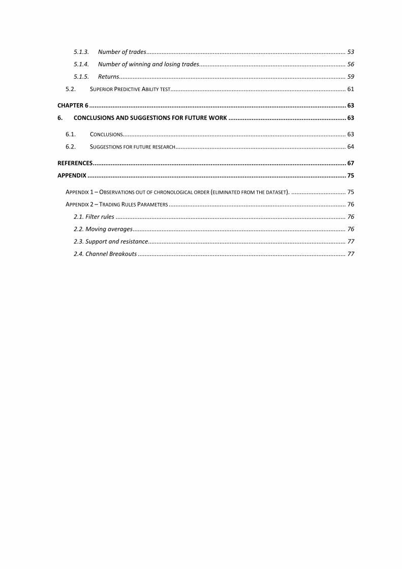
FIGURE 15 - MEAN NUMBER OF TRADES BY YEAR, FOR THE SUPPORT AND RESISTANCE GROUP. ........................................... 55
FIGURE 16 - MEAN NUMBER OF TRADES BY YEAR, FOR THE CHANNEL BREAKOUTS GROUP. ................................................. 55
FIGURE 17 - MEAN NUMBER OF WINNING/LOSING TRADES BY YEAR, FOR THE FILTER RULES GROUP. .................................... 57
FIGURE 18 - MEAN NUMBER OF WINNING/LOSING TRADES BY YEAR, FOR THE MOVING AVERAGES GROUP. ........................... 57
FIGURE 19 - MEAN NUMBER OF WINNING/LOSING TRADES BY YEAR, FOR THE SUPPORT AND RESISTANCE GROUP. .................. 58
FIGURE 20 - MEAN NUMBER OF WINNING/LOSING TRADES BY YEAR, FOR THE CHANNEL BREAKOUTS GROUP. ......................... 58
FIGURE 21 – MEAN RETURN BY YEAR, FOR THE FILTER RULES GROUP. ............................................................................ 59
FIGURE 22 - MEAN RETURN BY YEAR, FOR THE MOVING AVERAGES GROUP. .................................................................... 60
FIGURE 23 - MEAN RETURN BY YEAR, FOR THE SUPPORT AND RESISTANCE GROUP. ........................................................... 60
FIGURE 24 - MEAN RETURN BY YEAR, FOR THE CHANNEL BREAKOUTS GROUP. ................................................................. 61


xiii
LIST OF TABLES
TABLE 1 - DATABASE NUMBER OF OBSERVATIONS BY YEAR. ........................................................................................... 32
TABLE 2 - NUMBER OF TECHNICAL TRADING RULES USED. ............................................................................................. 36
TABLE 3 – AVERAGE PROPERTIES BY TRADING FAMILY, FOR THE ENTIRE PERIOD. ................................................................ 45
TABLE 4 - COMPARISON OF THE AVERAGE TRADING DURATION FOR THE ENTIRE PERIOD, BY GROUP OF RULES. ........................ 53
TABLE 5 - SPA TEST RESULTS. ................................................................................................................................. 62


xv
LIST OF ACRONYMS AND ABREVIATIONS
CNBC - Consumer News and Business Chanel
DJIA – Dow Jones Industrial Average
EMH – Efficient Market Hypothesis
FIPS - Fixed Income Pricing System
FTSE 100 Index - Financial Times Stock Exchange 100 Index
FX - Foreign Exchange
GMT - Greenwich Mean Time
LSEG - London Stock Exchange Group
MIB30 - Milano Italia Borsa 30 Index
NASD - National Association of Securities Dealers
NASDAQ - National Association of Securities Automated Quotations
NYSE - New York Stock Exchange
S&P 500 – Standard and Poors 500
SPA test – Superior Predictive Ability test
SPDR – Standard and Poor’s Depository Receipts
UK - United Kingdom
USA – United States of America


CHAPTER 1 - INTRODUCTION 17
CHAPTER 1
1. INTRODUCTION
For most of its life, the field of finance as debated the question of market efficiency. The
discussion has started in the 1960s and until this day there is still debate, be it among
academics or practitioners, about the question of markets efficiency.
Among the scientific research on modern Finance those studies that are rated amongst the
most influential on the matter are the 1953 Maurice Kendall’s study that brought to light
the random movement of stock prices, coined as the random walk hypothesis (Kendall,
1953), and 1965 Eugene Fama’s work presenting, for the first time, the concept and
definition of efficient markets. As he puts it, in an efficient market information is reflected
on market prices, and thus prices should follow a random walk (Fama, 1965). Although
this theory would later suffer some alterations by its own author (Fama, 1970, 1991), the
underlying idea of the Efficient Market Hypothesis (EMH) is that a market is efficient if
the prices fully reflect all available information.
Moreover, Fama defines the EMH in three forms, the weak form that implies that markets
are efficient, reflecting all market historical information, the semi-strong form according to
which the market is efficient reflecting all publicly available information, and finally the
strong form that defines an efficient market in the sense that prices reflect all information
both public and private (Fama, 1970).
Through the decades that followed these theories have been put under scrutiny, with
several studies coming forward with contrary ideas. But in essence most of the academic
world accepts the EMH and the random walk hypothesis.
The same cannot be said about practitioners, laying here the great discrepancy between the
two sides of this area. Some market participants state that it is possible to predict the
movements of the market just by taking into account the past prices and movements
(technical analysis), which goes against the EMH.

18 CHAPTER 1 - INTRODUCTION
For example, studies on the matter, such as Carter and Van Auken (1990), Allen and
Taylor (1992), Lui and Mole (1998), and Oberlenchner (2001), consistently find that the
practitioners emphasize technical analysis over fundamental analysis the shorter the time
frame of forecasting. According to Marshall et al. (2008) practitioners place twice as much
importance on technical analysis for intraday horizons when compared with a longer
horizon of one year.
Consequently, it is only fitting that given the referred importance that practitioners deposit
on technical trading, especially on short periods of time, and the abundance of studies,
even those using intraday data, that find evidence for and against, the question of the
profitability of the technical analysis, and thus the markets efficiency, remains current for
both academics and market participants.
Accordingly, with this study, I investigate if there is a technical trading rule, from a set of
well-known trading rules, which can generate abnormal returns on the Financial Times
Stock Exchange (FTSE) 100 Index from the period starting in January 2000 to December
2010.
In order to accomplish those goals, from the several existing ways to test the weak form of
the EMH, I define and implement trading rules that use past information and test if they
provide abnormal returns (Lo et al., 2000; Jegadeesh, 2000).
Finally, in order to test the statistical significance of the results I use the Superior
Predictive Ability test by Hansen (2005).

CHAPTER 2 – LITERATURE REVIEW 19
CHAPTER 2
2. LITERATURE REVIEW
The knowledge about human behavior when one is faced with investment decisions has
evolved substantially since Keynes’s animal spirits theory, resulting from the book entitled
The General Theory of Employment, Interest and Money (Keynes, 1936). This theory
conveys that the investor takes decisions based on random-like thinking, in such way that
the stock market is comparable with a beauty contest. More precisely, Keynes says that
“most, probably, of our decisions to do something positive, the full consequences of which
will be drawn out over many days to come, can only be taken as a result of animal spirits,
of a spontaneous urge to action rather than inaction, and not as the outcome of a weighted
average of benefits multiplied by quantitative probabilities”.
In fact, this chapter follows with a review of the literature on the area which is subject to
this study, intraday trading, more specifically the part dedicated to technical analysis. Since
this is narrowly connected with the definition of the market efficiency and the random
walk hypothesis I also present a small recap of the state of knowledge on the subject.
Consequently I start by presenting a brief summary of the academic advances that led to,
and followed, the formulation of the random walk hypothesis, and the EMH. More
precisely, its origin, motivation, definition and the evolution on the literature about the
subject, that presents strong arguments in favor and against it.
To end the chapter, I define and present statistical tests that account for data snooping used
for studies in financial economics.

20 CHAPTER 2 – LITERATURE REVIEW
2.1. Modern Finance, the random walk hypothesis and EMH
The history of scientific research on the matter of the behavior of investors goes a long
way back. According to Sewell (2011) it can be traced as far as the 16th
century, when
Girolamo Cardano, an Italian mathematician, wrote that “the most fundamental principle
of all in gambling is simply equal conditions, e.g. of opponents, of bystanders, of money,
of situation, of the dice box, and of the die itself. To the extent to which you depart from
that equality, if it is in your opponents favor, you are a fool, and if in your own, you are
unjust”. Since then the evolution of the scientific knowledge on the matter has been
constantly evolving.
However, on the subject of the modern finance and more precisely the subject of technical
analysis and the efficiency of the markets, most changes on the perception that we have
about the role of the investor in the markets has occurred in the 1950s, 1960s and 1970s,
fundamentally due to researchers such as Milton Friedman, Paul Samuelson, Maurice
Kendall, Eugene Fama, Kenneth French, and Michael Jensen.
The most significant advances on this field started in 1953, when Milton Friedman pointed
out that, due to arbitrage, the case for the EMH (which only latter would be presented and
defined as we know it now) can be made even in situations where the trading strategies of
investors are correlated (Friedman, 1953).
In the same year the first effort was made to make public the randomness of the movement
of stock prices, by Maurice Kendall. He analyzed 22 price-series at weekly intervals and
found that they were random (Kendall, 1953).
Later on, around 1955, it was credited to Louis Bachilier’s work on his PhD in
mathematics from 1900, later published in book form entitled The Game, the Chance and
the Hazard (translated from the original Le Jeu, la Chance et le Hasard) from 1914, a first
insight on the theory presented in 1953 by Kendall (Bernstein, 1992).
Effectively, according to Bachelier, “past, present and even discounted future events are
reflected in market price, but often show no apparent relation to price changes” and “if the
market, in effect, does not predict its fluctuations, it does assess them as being more or less
likely, and this likelihood can be evaluated mathematically” (Dimson and Mussavian,
2000).
Nevertheless, the first criticism to the random walk hypothesis did not take long to appear.
In 1961, Houthakker resorted to stop-loss sell orders, finding patterns on the prices, and
finding also leptokurtosis, nonstationarity and non-linearity (Houthakker, 1961).

CHAPTER 2 – LITERATURE REVIEW 21
In the year that followed, Mandelbrot suggested that the tails of the distribution of returns
follow a power law (Mandelbrot, 1962). Cootner went as far as suggesting that the stock
market do not follow a random walk (Cootner, 1962), and Osborne found out that stocks
tend to be traded in concentrated bursts, which is a deviation from a simple random walk
(Osborne, 1962).
For some of those criticisms there are possible explanations within the framework of the
random walk hypothesis. For example, the model for error clustering by Berger and
Mandelbrot (1963) serves as justification for the Mandelbrot’s critique in the previous year
(Sewell, 2011), and the spectral analysis on market prices made by Granger and
Morgenstern (1963) allowed them to conclude that short-run movements of the series obey
the simple random walk hypothesis.
The situation described before persisted in the subsequent years, with the arrival of several
studies in favor or against the random walk hypothesis and the EMH (Bernstein, 1992; Lo,
1997; Dimson and Mussavian, 1998; Farmer and Lo, 1999; Sewell, 2011).
The most prominent works in favor of such theories began with Eugene Fama’s discussion
of Mandelbrot’s work in previous years, namely the stable paretian hypothesis, concluding
that the tested market data conforms to the distribution (Fama, 1963).
Godfrey et al. (1964) tested the random walk hypothesis on the stock market, concluding
that it is the only mechanism that is consistent on describing the “unrestrained pursuit of
the profit motive by the participants in the market”.
In the following year, Eugene Fama reviews previous studies and concludes that there is
strong evidence in favor of the random walk hypothesis, presenting, for the first time, a
definition of the concept of efficient markets (Fama, 1965).
Still in 1965, Paul Samuelson contributes for an extension on the perception of the markets
efficiency, focusing on a martingale process instead of a random walk, and stating that “in
competitive markets there is a buyer for every seller. If one could be sure that a price
would rise, it would have already risen” (Samuelson, 1965).
This is followed by 1966 Mandelbrot’s work, where he concludes that in competitive
markets with rational risk-neutral investors, returns are unpredictable, thus prices follow a
martingale (Mandelbrot, 1966).
In 1967, Roberts introduces for the first time the distinction between weak and strong form
of the market efficiency (Roberts, 1967). While Fama et al. (1969), considered the first
ever event study, concluded that the stock markets are indeed efficient.

22 CHAPTER 2 – LITERATURE REVIEW
Fama (1970) defined an efficient market as a market where prices reflect all the available
information, also making the distinction between weak form, semi-strong form and strong
form of the EMH.
The decade that followed brought some other relevant studies, from which stand out
Makiel (1973), Samuelson (1973), Grossman (1976), Fama (1976), and Jensen (1978). The
last one introduced the distinction between the statistical and the economic efficiency.
Jensen stated that a market is efficient with respect to a specific information set, if it is
impossible to make economic profits by trading on the basis of that information set.
Adding that “by economic profits, we mean the risk adjusted returns net of all costs”
(Jensen, 1978).
In other words, Jensen intended to show that even if one can prove a market is inefficient
by analyzing its prices, the same conclusion can be proved wrong when an investor tries to
replicate the techniques and processes evaluated, since there are costs associated to each
buy and sell operation. This is of most importance as most of studies relied on an approach
that not accounted for costs and, mistakenly, draw conclusions against the EMH from the
results obtained.
These studies were followed in the next decades by publications of the like of Black
(1986), Eun and Shim (1989), Fama (1991, 1998), Makiel (1992, 2003), Metcalf and
Malkiel (1994), Chan et al. (1997), Lewellen and Shanken (2002), Chen and Yeh (2002),
Lo (2008), and Yen and Lee (2008). All of them favoring the case of the EMH and the
random walk hypothesis.
Even more recently, Bajgrowicz and Scaillet (2012) attest on favor of the markets
efficiency. In this study the authors test the performance of technical trading rules on the
Dow Jones Industrial Average (DJIA) index in the period from 1897 to 2011, using the
false discovery rate (FDR), a new approach to data snooping, and proving wrong Brock et
al. (1992), a similar study that used basically the same database and technical trading rules,
but that led to different conclusions.
In the opposite side of the discussion there were also several studies trying to refute the
random walk hypothesis as well as the EMH.
Indeed some of the most notable work, at an initial stage, was done by Sydney S.
Alexander (Alexander, 1961, 1964), who concluded that the Standard and Poors (S&P)
industrial index did not follow a random walk. Being followed by De Bondt and Thaler
(1985), study where the authors discovered overreaction on the stock prices. This study is
considered, by many, as the start of the behavioral finance research.

CHAPTER 2 – LITERATURE REVIEW 23
Additionally, Eugene Fama and Keneth French find, in 1988, that 25 to 40 percent of the
variation of long horizon returns is predictable from past returns (Fama and French, 1988).
Whereas, Chan et al. (1996) found evidence that markets respond gradually to new
information leading to periods of mispricing.
An extended number of other studies, also making the case against the EMH, accompanied
these works.
In the decades of 1960 an 1970 the most notable works were accomplished by Steiger
(1964), Granger and Morgenstern (1970), Kemp and Reid (1971), Beja (1977), and Ball
(1978).
In the following decades the critiques rose in number with the works of the like of
Grossman and Stiglitz, (1980), LeRoy and Porter (1981), Stiglitz (1981), Shiller (1981,
1989, 2000), Roll (1984), Summers (1986), Keim and Stambaugh (1986), French and Roll
(1986), Lo and MacKinlay (1988, 1999), Cutler et al. (1989), Laffont and Maskin (1990),
Lehmann (1990), Jegadeesh (1990), Chopra et al. (1992), Bekaert and Hodrick (1992),
Jegadeesh and Titman (1993), Huang and Stoll (1994), Haugen (1995, 1999), Bernstein
(1999), and Shleifer (2000) only to mention a few.
Even in the most recent years literature still emerges against the EMH (Wilson and
Marashdeh, 2007; Lee et al., 2010).
This schism and continuous exchange of arguments is well summarized by Schwert in the
article Anomalies and Market Efficiency, where he identifies the documented anomalies,
finding that most of them disappeared, perhaps revealing some ephemeral market
inefficiencies, finding also other new anomalies (Schwert, 2002).
2.2. Intraday technical analysis
Effectively one can conclude that this is an area of great debate and thus of great
importance in Finance, be it for academics or practitioners.
In fact here lies the great discrepancy between the two sides of this area. In one hand we
have the academics who, despite the divergences made clear above, always favored the
idea that it is not possible to predict future price movements using the past price
movements (technical analysis). In the other hand there are the market participants among
whom there is the perception that it is possible to predict the movements of the market just
by taking into account the past prices and movements.

24 CHAPTER 2 – LITERATURE REVIEW
The same statute of schism is not applicable to fundamental analysis. According to Lo et
al. (2000), “it has been argued that the difference between fundamental analysis and
technical analysis is not unlike the difference between astronomy and astrology”,
complementing that “among some circles, technical analysis is known as “voodoo
finance”.
Additionally, Lo et al. (2000) point out that the explanation behind this difference of
treatment could be associated with the “unique and sometimes impenetrable jargon used by
technical analysts”, adding that “some of which has developed into a standard lexicon that
can be translated”. Be it as it may, the truth is that the discrepancy of treatment of the two
approaches is very different depending if the subject is an academic or market participant.
The disposition of academics towards technical analysis, or charting as it is also referred, is
well put by Makiel: “Technical analysis is anathema to the academic world. We love to
pick on it. Our bullying tactics are prompt by two considerations: (1) the method is
patently false; and (2) it is easy to pick on. And while it may seem a bit unfair to pick on
such a sorry target, just remember: it is your money we are trying to save” (Makiel, 1981).
Regardless, studies on the matter, such as Carter and Van Auken (1990), Allen and Taylor
(1992), Lui and Mole (1998), and Oberlenchner (2001), consistently find that the market
participants emphasize technical analysis over fundamental analysis the shorter the time
frame of forecasting. According to Marshall et al. (2008) they place twice as much
importance on technical analysis for intraday horizons when compared with a longer
horizon of one year.
This notion is a lot more relevant when authors such as Manahov et al. (2014) state that the
discrepancy between academic studies related to technical trading, in the Foreign
Exchange (FX) market, and practitioners is largely due to the fact that academic research
limits their trading strategies to daily observations.
Having that in mind, the study of intraday technical analysis becomes of great importance
on the matter of market efficiency.

CHAPTER 2 – LITERATURE REVIEW 25
To the best of my knowledge, the first study published using a higher trading frequency
came up in 1985 entitled An investigation of transactions data for NYSE stocks by Wood et
al. (1985). On it the authors tested a large sample of New York Stock Exchange (NYSE)
stocks, examining them on a minute-by-minute transaction data period over two time
periods, from September 1971 to February 1972 (data from 946 stocks) and the entire
calendar year of 1982 (data from 1138 stocks). They found evidence of differences in
return distributions among trades occurring overnight, during the first thirty minutes of
trading day, at market close and during the rest of the day. Moreover, they realize that all
positive returns are earned during the first thirty minute of the trading day and at the
market close, and that in the rest of the day market returns are normally distributed and
autocorrelation is substantially reduced (Wood et al., 1985).
Almost a decade later, Froot and Perold (1995) examine short-run autocorrelation of stock-
index returns, finding that it has been declining dramatically in recent years. Over the
period of 1983-1989 the returns on S&P 500 went from being highly positively correlated
to practically uncorrelated. The paper shows that positive index autocorrelation found in
earlier studies was a result of high autocorrelation on the 1960s and 1970s, vanishing by
the late 1980s. The explanation for such is attributed to “inefficient processing of market-
wide information”, pointing out “that recent technological and institutional improvements
in the processing of this information has removed much of the autocorrelation”. In their
study the authors used 15 minute returns, and they did not test for data mining.
Los (1999) tests and concludes that none of nine Asian currencies exhibited complete
efficiency during the year of 1997. The author tested the stationarity and the serial
independence of the price changes on minute-by-minute data for nine currencies during the
period starting in January 1, 1997 to December, 30 1997, and, as Froot and Perold (1995),
he did not conduct data snooping tests.

26 CHAPTER 2 – LITERATURE REVIEW
Already on the new millennium, Busse and Green (2002) examine the influence of live TV
analysis on individual stocks during the trading day. In that regard they test 322 individual
stocks featured on Morning Call and Midday Call of the network CNBC - Consumer News
and Business Chanel (both programs are highly regarded by market participants). They use
the simple mean of the intraday price changes and conduct the nonparametric bootstrap
algorithm from Barclay and Litzenberger (1988) to determine the statistical significance.
The conclusions to which they arrive are that in one hand the prices adjust within seconds
of the initial mention, and in the other hand, traders who execute within 15 seconds of the
initial mention make small but significant profits by trading on positive reports. In this
study, the authors focus is not the market efficiency per se, rather the time of response
from prices to news and big announcements. Even though, the fact that at a given period of
time there are investors who can profit from stock prices, taking only into account past
patterns (in this case a specific TV show indication and the market reaction to it), attests
for market inefficiencies.
In the ensuing year, Hotchkiss and Ronen (2002) go on favor of the market efficiency,
since they conclude that the bond market is quick to incorporate information, even at short
return horizons. To get to that conclusion the authors used a dataset based on daily and
hourly transactions for 55 high-yeld bonds included on the Fixed Income Pricing System
(FIPS) from the National Association of Securities Dealers (NASD) between January 1995
and October 1995.
An opposite view is portrayed by Cassese and Guidolin (2004), once they examine the
pricing and informational efficiency of the most important Italian stock index, the Milano
Italia Borsa 30 (MIB30), in the period from April, 6 1999 to January, 31 2000. They found
it quite inefficient, with a numerous percentage of the analyzed data (up to 40% of the
data) violating non-arbitrage condition. Although, in order to reach to that conclusion, the
authors did not account for transaction costs, they state that, even if transaction costs are
considered, there are significant arbitrage opportunities.
Chordia et al. (2005) study the stocks listed on the NYSE from 1993 to 2002 and conclude
that daily returns are not serially correlated while order imbalances on the same stocks are
highly persistent. The authors add that this is due to the fact investors react promptly to
order imbalances, taking 5 to 60 minutes in the process, also that short-term (5 minutes)
return predictability has been declining and that market liquidity and efficiency are
positively correlated. The authors did not conduct any significant test to control for data
mining.

CHAPTER 2 – LITERATURE REVIEW 27
At their turn, Marshal et al. (2008) conclude that, for the Standard and Poor’s Depository
Receipts (SPDR), intraday technical analysis is not profitable. The authors tested 7846
technical trading rules on data from 2002 and 2003, and controlled for data snooping
through the application of the Brock et al. (1992) bootstrap methodology and the Sullivan
et al. (1999) reality check test.
Chordia et al. (2008) perform a study on a sample of large and actively traded NYSE firms
over a period of ten years (from 1993 to 2002) complemented later by Chung and Hrazdil
(2010) on a broader study that included all NYSE traded firms. Both papers focus on the
dynamics between liquidity and market efficiency, leading to the (same) conclusion that
there is positive correlation between the two variables, being the effect amplified during
periods of information release. In other words, according to both studies, liquidity
enhances market efficiency.
A few years later, Scholstus and Dijk (2012) tried to find the relationship between the
speed of trading and its performance. In order to accomplish it, the authors used data from
S&P500, National Association of Securities Automated Quotations (NASDAQ) 100 and
Russell 2000, from the period from January 6 of 2009 to September 30 of 2009. The study
revealed that speed has an important role on the performance of the technical trading rules,
being the ones with lower delays those with better (positive) average returns.
Other recent study that gave ground to the EMH was published in 2013. The authors tested
the intraday predictive power using technical trading strategies on the 30 constituents of
the DJIA index. They concluded that there is no abnormal return over the buy-and-hold
strategy (Duvinage et al., 2013).
Furthermore, according to Chaboud et al. (2014), that focused on high frequency
algorithmic trading on the FX, there is an improvement on price efficiency and a reduction
on arbitrage opportunities associated primarily with automated (computer generated)
trading.
Manahov et al. (2014) found evidence of statistical and economical significance of excess
returns on the FX, even after accounting for the transaction costs. In this study, the authors
did not conduct a robustness test on their results.
Indeed the existing literature on intraday technical analysis seems to be skewed on favor of
the EMH and the random walk hypothesis, since most of studies point out that, after the
consideration of transaction costs and data snooping measures, there are no trading
strategies that can, consistently, beat the market, even considering trading strategies with
shorter time frames.

28 CHAPTER 2 – LITERATURE REVIEW
Nonetheless, the fact that there is still some literature that try and succeed in finding flaws
to the EMH and the random walk hypothesis, attest for the validity, even nowadays, of the
question of the markets efficiency.
2.3. Data snooping measures
According to Leamer (1978) the empirical tests in financial economics which are free from
data instigated biases are close to none. So in this kind of studies there is always the risk
that the results are driven by data mining.
Following the same path, Lo et al. (1990) states that tests of financial asset pricing models
may result in misleading inferences when properties of the data are used to construct the
test statistics. Such tests are often based on returns to portfolios of common stock, where
portfolios are constructed by sorting on some empirically motivated characteristic of the
securities such as market value of equity.
Dimson and Marsh (1990) finds that “even apparently innocuous forms of data-snooping
significantly enhance reported forecast quality, and that relatively sophisticated forecasting
methods operated without data-snooping often perform worse than naive benchmarks”.
Moreover, Brock et al. (1992) adds that “the more scrutiny a collection of data receives,
the more likely “interesting” spurious patterns will be observed”.
In order to illustrate the conundrum of data snooping, Bajgrowicz and Scaillet (2012) use a
good anecdote. They state the following, “imagine you put enough monkeys on typewriters
and that one of the monkeys writes The Iliad in ancient Greek. Because of the sheer size of
the sample, you are likely to find a lucky monkey once in a while. Would you bet any
money that he is going to write The Odyssey next?”.
The same argument can be applied to trading rules. If one looks hard enough, a trading rule
will eventually generate abnormal returns, even if it lacks predictive ability.
Indeed, a good part of the literature evidence in favor of the predictive ability of technical
trading rules can be draw back to studies made without accounting for data snooping
biases. This is an issue that is transversal to most studies that were undertaken in the past,
for both intraday and daily datasets.
Examples of this effect are Brock et al. (1992), Levich and Thomas (1993) and Osler and
Chang (1999).
The possibilities to avoid such problems have been under greater discussion for the past 30
years, with special focus in the past decade.

CHAPTER 2 – LITERATURE REVIEW 29
In fact, Brock et al. (1992) presents a study were the authors conduct a test of significance
for the set of technical trading rules employed, through the use of bootstrap.
Diebold and Mariano (1995) produces a test intended to compare forecast, but actually has
been largely used to compare models. However, Giacomini and White (2003) refers that
this test is conservative when applied to short-horizon forecasts, since the model
parameters are estimated using a rolling window of data, rather than an expanding one.
Other example of a well documented and widely used test is the reality check for data
snooping (RC) of White (2000). The author created a test for comparing multiple
forecasting models or rules. This procedure compares the total number of rules or models
under estimation to a benchmark, and tests if the benchmark is significantly outperformed
by any model used in that comparison.
This test would be refined by Hansen (2005), in the sense that it accounts for the variation
of the outperformance of each model compared with the benchmark. This relative
calculation results in a test less sensitive to the inclusion of poor and irrelevant alternatives.


CHAPTER 3 - DATA 31
CHAPTER 3
3. DATA
For the purpose of the study, I used the intraday database on the FTSE 100 Index available
on the School of Economics and Management, at the University of Minho. This database
aggregates a total of 11 years of data, from January 2000 until December 2010, which,
compared to the data commonly used on existing literature, is a considerable time frame,
being, from a theoretical point of view, large enough to deliver robust results.
On the remainder of this chapter, I present a summary of the data on the database, some
checks that were done in order to guarantee that there are no values mistakenly
incorporated in the database, the aggregation of the data into lower frequencies, and,
finally, the description of the risk free used.
3.1. Summary
The database has a total of 20,188,968 observations, distributed annually as showed on
Table 1.
More precisely, from 2000 to 2008 there are about half a million observations each year,
whereas in the last two years that number increases for more than 1.3 million in 2009, and
more than 14 million in 2010. This happens because prior to December 2009 prices were
made recorded on a 15 seconds interval (approximately), and from that date on prices
entries were made with greater frequency (they were registered as changes occurred).

32 CHAPTER 3 - DATA
Table 1 - Database number of observations by year.
Year Number of observations
2000 507,628
2001 463,828
2002 461,734
2003 471,774
2004 495,214
2005 495,707
2006 498,224
2007 455,235
2008 516,510
2009 1,331,934
2010 14,491,180
3.2. Data verification
According to the London Stock Exchange Group (LSEG) the trading hours for the FTSE
100 index starts at 08:00 and ends at 16:30 Greenwich Mean Time (GMT), except on the
last working day preceding Christmas and New Year’s Eve, when it opens at 08:00 and
closes at 12:30 GMT (London Stock Exchange Group - Official website of the London
stock exchange, 2016).
Accordingly, the first and last daily observations on the database are presented on Figure 1
and on Figure 2, respectively.
Regarding the first daily observation, as expected, most of them occur precisely at 8 am.
Even though, there are a few days where the first observation is not at 8 am or at an
approximate time. In fact some days have the first entry from as late as 10 am. Besides that
there are other values worthy of attention, exactly 3 prices which are registered past 12:00.
On the same premise, the last daily observation (represented on Figure 2) was also verified.
Here, the observations are not in line with the first ones in each trading day. There a lot
more discrepancies on the last recorded price.
For both cases, I conduct some verifications. I start by verifying if there are any reasons for
those abnormal time stamps, and found that there are technical reasons for some of them.
Then I proceed to compare the prices on the database to the prices on other database,
namely the Thomson Reuters/Datastream database, and concluded that there are no major
errors on the database and therefore decided to keep all records.

CHAPTER 3 - DATA 33
I also checked if there are any records outside trading days.
In order to do that, I resorted to the institutional website of the United Kingdom (UK)
government, obtaining the bank holidays on which it is not supposed to exist observations.
After verification, no observations were found on weekends or holidays (UK Government.
Official website of the UK government services and information, 2016).
Furthermore, there are a few working days when there are no observations, for example the
9/11 terrorist attacks on the World Trade Center.
Next, I checked for the existence of observations off chronological order. Indeed there
were 81 prices that entered off the correct chronological order. Those entries were
eliminated from the dataset.
Figure 1 – First daily observation.

34 CHAPTER 3 - DATA
Figure 2 – Last daily observation.
3.3. Data aggregation
When looking to Table 1 the main characteristic from the data that stands out is the
different number of observations in the last two years compared to the previous ones. Such
difference, as said before, is due to the change on the time frequency of the records of
index values in the database.
Since all trading rules considered assume that returns are calculated over the same time
period, I aggregated returns to a five minute interval.
The time frame of 5 minutes was chosen in accordance to other studies, such as Marshall et
al. (2008).
3.4. Risk free rate
For the purpose of the analysis, the risk free rate used was obtained from the
Thomson/Reuters database. The risk free rate here considered is the pound overnight
middle rate provided by the Bank of England.

CHAPTER 4 - METHODOLOGY 35
CHAPTER 4
4. METHODOLOGY
In order to find if there is a technical trading rule that can generate abnormal, risk adjusted,
returns, in other words, to test the weak form of the EMH, there are three common
approaches. One is to find and test some kind of calendar regularity or anomaly; another
form consists in analyzing the properties of the series (e.g. sample correlations, run tests,
variance ratio tests); and yet another approach is to implement trading rules that use past
information.
In fact, I use the later. In accordance, I define and implement trading rules that use past
information and test if they provide abnormal returns (Lo et al., 2000; Jegadeesh, 2000).
Effectively, the set of technical trading rules employed on the study were the ones
purposed by several other studies, e.g. Sullivan et al. (1999), Marshall et al. (2008),
Bajgrowicz and Scaillet (2012). Those techniques are known previously to the period of
the data under analysis, hence avoiding data mining issues (Marshall et al., 2008).
Finally, for the test of profitability it is often used the Brock et al. (1992) bootstrapping
methodology, the White’s Reality Check bootstrapping technique for data snooping
(Sullivan et al., 1999, 2001, White, 2000), and the Superior Predictive Ability test (Hansen,
2005).
On this study I use the Superior Predictive Ability test (Hansen, 2005), from now on
referred as SPA test, since it is more powerful and less sensitive to the inclusion of poor
and irrelevant alternatives, when compared to the other approaches (Hansen, 2005).
Indeed, in the reminder of this chapter I present definitions for the technical trading rules
employed, the measurements of performance and then, in more depth, the test to assess the
statistical significance of the results.

36 CHAPTER 4 - METHODOLOGY
4.1. Technical Trading Rules
Regarding the technical trading rules employed on this study, I looked for rules that were
of common knowledge prior to the time frame of the data under analysis. This, according
to Lakonishok and Smidt (1988), Lo and MacKinlay (1990), and Pesaran and Timmerman
(1995), tends to avoid data snooping bias. This is well put by Marshall et al. (2008), “the
application of new trading rules, or new specifications of existing trading rules, to
historical data introduces the chance of data snooping bias. It is quite possible that the rules
have been tailored to the data series in question and are only profitable because of this”.
Effectively, the rules employed were from four families of trading rules, filter rules,
moving averages, support and resistance, and channel breakouts, used on several studies on
the subject, such as Brock et al. (1992), Sullivan et al. (1999), Marshall et al. (2008) and
Bajgrowicz & Scaillet (2012).
On Table 2 are presented the number of technical trading rules used on the study. A total of
5680 rules were tested, 600 of the filter rules, 3780 of the moving averages, 180 of the
support and resistance and 1120 of the channel breakouts family.
Table 2 - Number of technical trading rules used.
Family of trading rules Number of rules
Filter rules 600
Moving averages 3780
Support and resistance 180
Channel breakouts 1120
Total 5680

CHAPTER 4 - METHODOLOGY 37
4.1.1. Filter rules
In order to define and implement the trading rules from the filter rules family, first used by
Alexander (1961), I resorted to Fama and Blume (1966) and to Sullivan et al. (1999). Both
papers state that when a daily closing price of a security moves up or down at least x per
cent (being x a value to be defined) one should buy and hold that security, or short sell,
respectively. From there, each subsequent day, one should check the closing price,
watching for two different possibilities, if the price goes down (or rises on the second
scenario) for more than x per cent the following action should be to sell (buy) the security,
otherwise if the price goes up (down) it becomes the price of reference for it to be
compared to the closing price in the next day, on all other price movements the position
remains unchanged.
Since the database used is not composed of daily prices, but rather of intraday prices, the
definitions cited for daily prices should be adapted accordingly. So the “closing price” is
assumed as the last price prior to the current period under consideration.
Additionally to the standard filter rules described, there are some variations that I consider
for this study.
Starting with the price of reference, which on the standard form is the subsequent high
(low) if the position is long (short), it can be also defined as the most recent price that is
greater (less) than the e previous prices.
I also consider the possibility of a neutral position to be taken when the price decreases
(increases) y percent from the previous high (low).With y less than x.
Finally, another variation to the standard filter is imposed by allowing a position to be
held, be it long or short, for a given, c, number of periods, ignoring all other signals
generated during that period.

38 CHAPTER 4 - METHODOLOGY
4.1.2. Moving averages
Moving averages are among the groups of trading rules with wider use and discussion on
technical trading literature. Its usage dates to the 30s, when Gartley (1935) mentioned that
“in an uptrend, long commitments are retained as long as the price trend remains above the
moving average. Thus, when the price trend reaches a top, and turns downward, the
downside penetration of the moving average is regarded as a sell signal… Similarly, in a
downtrend, short average. Thus, when the price trend reaches a bottom, and turns upward,
the upside penetration of the moving average is regarded as a buy signal”.
Brock et al. (1992) stated that the idea behind this particular technique is to smooth out an
otherwise volatile series.
Accordingly, a buy signal is generated when the short-period moving average rises above
the long-term moving average, and vice-versa, when the short-period moving average falls
below the long–period moving average a sell signal is generated. Therefore, the portfolio is
always on the market, either with long or short positions.
As before, some variations of the standard moving averages were considered.
The first variation was introduced by applying a band filter on the moving average, which
resulted on the reduction of the number of buy and sell signals by eliminating what Brock
et al. (1992) describes as “whiplash” signals when the long and short period moving
averages are close. In other words, the fixed percentage band filter requires the buy or sell
signal to exceed the moving average by a fixed multiplicative amount, b.
The second variation considered was the time delay filter, which requires the buy or sell
signal to be the same for a given number of periods, d. Only if a signal repeats itself for a
number of periods equal to d, action is taken in order to act according to the signal.
The third and final variation is the same as the one used for the Filter Rules (on 4.1.1). A
position is held for c periods, ignoring all other signals during that period.
4.1.3. Support and resistance
Support and resistance is another group of technical trading rules with a well documented
usage. According to Sullivan et al. (1999) it can be traced to Wyckoff (1910).

CHAPTER 4 - METHODOLOGY 39
In its simplest form, a buy signal is generated when the price rises above the resistance
level (local maximum). The logic behind this rule relies on the belief that many investors
are willing to sell at a peak, leading to a potential selling pressure that causes resistance to
the price penetration of the previous maximum. Though, if the price breaks through this
pressure point and surpasses the resistance level, this should be perceived as a buy signal
(Brock et al., 1992).
The same reasoning can be followed for sell signals. If the price drops below the support
level (local minimum) a sell signal is generated.
As for the other groups of trading rules, I implemented some variations to the basic form
defined above. Those were the same implemented for the moving averages, a fixed
percentage band filter, b, a time delay filter, d, and position holding for c periods.
4.1.4. Channel breakouts
Sometimes referred to as the Dow line or Dow Theory, this technical trading rule has been
around for more than a century. It was developed by Charles Dow, hence the titles coined
to the rule, in the late years of the 19th
century.
The rule, later refined by William Hamilton (Hamilton, 1922) and better described by
Robert Rhea (Rhea, 1932), states that one should buy when the closing price exceeds the
channel and sell when the price moves below the channel. The channel occurs when the
high over the previous n days is within x percent of the low over the previous n days, not
including the current price (Sullivan et al., 1999).
Again, the previous definitions are specifically focused for daily prices. For this study
some considerations are made resulting in the definition that follows: if the maximum price
of the previous n periods is less or equal to (1+x) times the minimum price of the same
period, a channel occurs (1). Thus, and only after the previous condition is met, an
evaluation is made to infer if the position to be held is long or short. The first occurs if the
current price is higher than the maximum price of the previous n periods (2), the second
when the opposite is verified (3).
)1(PrminPrmax: xiceiceChannel , (1)
Where maxPrice is the highest price of the previous n periods,
minPrice is the lowest price of the previous n periods.

40 CHAPTER 4 - METHODOLOGY
iceicecurrent PrmaxPr (2)
iceicecurrent PrminPr (3)
Once again, variations of this basic form are considered. Namely, the fixed percent band
filter, b, and the fixed number of periods, c, holding the same position.
4.2. Performance measurement
The results for the study were obtained following a simple algorithm, each trading rule
generates an investment signal, 1, 0 or -1, respectively for a long, neutral and short
position. According to Bajgrowicz and Scaillet (2012), other ways to manage the signals
could be employed, but since the conclusion would be the same and this signals
interpretation are fairly intuitive, I opted for this approach.
Regarding the performance measurement of those returns, I followed the relevant literature
on the matter and used the risk free rate as benchmark (Sullivan et al., 1999 and on Brock
et al., 1992), gauging if the rules are able to generate absolute returns. The risk free rates
used are the overnight interest rates given by the Bank of England.
In detail, when the signal generated indicates to buy (1), I buy the index at the current
price, if instead the signal is for a sell (-1), I go short on the index, and otherwise the
portfolio is outside the market. For all that options, the portfolio is compared to the option
of earning the risk free rate for the entire period.
Furthermore, as seen on Marshall et al. (2008), I use the index as a benchmark as well.
This is accomplished by doing the same as for the risk free rate, although in this approach
the comparison is made over a long position on the index for the whole period.
Finally, concerning the performance criteria, I use the simple mean return.
4.3. Data snooping measures
In order to avoid spurious patterns in the results I use the Superior Predictive Ability test
by Hansen (2005). This consists in an evaluation of the trading rules in the context of the
total group of rules, which reduces the significance of a rule if it is the only one presenting
positive abnormal returns. In this case the null hypothesis is that the performance of the
best trading rule is no better than the benchmark performance.

CHAPTER 4 - METHODOLOGY 41
To be more specific, the SPA test checks if there is a trading rule with larger expected
profit than the current rule.
Take δk,t-1 (where k = 0, 1, …, m) as the set of possible decision rules (long, short or
neutral) at time t-1, which are evaluated with a loss function, L(ξt, δt-h), where ξt is a
random variable that represents the aspects of the decision problem that are unknown at the
time the decision is made. A given trading rule profit, πk,t, is given by δk,t-1rt, where rt is the
return on the asset in period t.
In this study the random variable, ξt, assumes the value of rt, what makes the loss function,
L(ξt, δt-h), equal to the profit of the benchmark, δk,t-1 rt (long position on the index).
Given that, the performance, d, of the rule k, at time t, relative to the benchmark, is given
by the following expression,
),(),(,,0, htkthtttk
LLd , .,...,1 mk (4)
And the null hypothesis can then be as presented on (5), assuming an expected positive
value for the performance of rule k at time t.
00
H , with m (5)
Furthermore, the test statistic is given by
0,
ˆmaxmax
21
,...,1k
k
mk
SPA
n
dnT
(6)
Where 2ˆk
is some consistent estimator of )var( 21
2
kkdn .
And the estimator is given by
ndnk
c
k
kk
dloglog2ˆ2
11ˆ
, k=1,…,m (7)
Where
ndnkk
loglog2ˆ21
1
is the indicator function.

42 CHAPTER 4 - METHODOLOGY
The test distribution is estimated by the stationary bootstrap of Politis and Romano (1994).
The first step is to create time-series samples of the differences, and then calculate their
sample average,
n
t
tbbdnd
1
*
,
1* , b=1,…,B (8)
The test statistic requires estimates of its variance, 2
k , for k=1,…,m. To obtain it under the
null hypothesis, the bootstrap variable must be recentered, about l ,
c or u by
)(*
,,
*
,, kitbktbkdgdZ ucli ,, , Bb ,...,1 , nt ,...,1 (9)
Where ),0max()( xxgl
, nx
ck
xxgloglog2)(
21)(
, and
xxgu
)( .
Finally the test statistic is given by
k
bk
mk
SPA
nb
ZnT
max,0max
*
,21
,...,1
*
, (10)
And the p-value is
1.
B
b
TT
SPA
Bp
SPA
n
SPA
nb
1
*
,
1
ˆ
(11)
Where the null hypothesis is rejected for small values. Thus obtaining three values, one for
each one of the estimators l ,
c and u .
For a more detailed description of the procedure of this test please refer to Hansen (2005)
and the references therein.

CHAPTER 5 – RESULTS AND ANALYSIS 43
CHAPTER 5
5. RESULTS AND ANALYSIS
The results of the trading rules can be analyzed in a multitude of ways. In particular, they
can be evaluated with and without benchmarks, with and without measures to forecast
accuracy, by group of rules, or by period.
Faced with those possibilities, the approaches that I choose are the ones that, in a
reasonable extent, in my opinion allow for an in depth analysis of the results.
Consequently, follows a brief presentation of the average annualized returns, the excess
returns obtained over both benchmarks, each made by year and for the entire period, and
for each category of trading rules.
Additionally, I extend the analysis by comparing the duration and the number of trades of
the best rule, the winning (trading rules that yield positive returns) and the losing rules
(trading rules that yield negative returns) in each of the trading categories.
Finally, the results obtained for the SPA test are presented.
5.1. Results for the average return criterion
5.1.1. Overview
The analysis of the results obtained for the entire period from January 2000 to December
2010, resumed on Table 3, allow to conclude that the filter rules family is the one with
higher average return, followed by support and resistance, channel breakouts and, finally,
by the moving averages family, which is the only group presenting a negative average
return.
Regarding the average return of the best rule in each family, the filter rules is also the
family with the best performing rule. The other families’ best rule have quite similar
values, being the support and resistance the one with the worst performance.

44 CHAPTER 5 - RESULTS AND ANALYSIS
In terms of the average duration of trade it is noticeable on Table 3 that the best performing
rule in each family has much lower duration than the entire family average, being the only
exception the filter rules, for which the duration of the best rule, although being smaller, it
is much more closer to the average duration of the whole family.
Contrarily, the number of trades presents the opposite trend. The average for the family is
lower than the number of trades used by the best rule. Once again, the discrepancy in
values is great with the exception of the filter rules.
Still regarding the number of trades, the losing rules use, on average, more trades than the
winning rules for 3 out of the 4 families. Only the channel breakouts winning rules are able
to use more transactions than the losing ones.
Additionally, Figure 3 reports the average returns in each year under analysis and then for
the entire period. The returns are annualized with no consideration of costs, no benchmarks
and without filtering for data mining.
At a first glance it is apparent the high average return of most rules of the filter rules
family, at least for the first three years, then the returns fade away and tend to be closer to
zero, as most rules from the other trading families.
On those first three years it is also noticeable that the group of rules belonging to the
channel breakouts are the ones, by what seems to be a large margin, with worst
performance overall. During that period, although there are a lot of rules on the moving
average family which present negative returns, there are quite a few rules with higher
returns than the best of the channel breakouts family.
In the fourth year, as previously referred, there seems to be a reduction on the average
return of most rules under the group of filter rules. The same can be said to occur to the
moving averages and to the support and resistance rules. The opposite can be said for some
rules of the channel breakouts, as they seem to improve.
In the next four years the general conclusion that arises is the same. The filter rules, the
moving averages and the support and resistance rules seem to decrease in returns, and most
of rules of the channel breakouts tend to grow.
In 2008 there is again some noticeable variation. Filter rules increase again in average
return, assuming again the only positive values and the highest returns.
Afterwards, in the next two years the average return absolute values tend to decrease, being
closer to zero in all families of trading rules.

CHAPTER 5 – RESULTS AND ANALYSIS 45
Finally, regarding the averages over the entire period of all trading rules tested, it is
possible to attest that the ones with higher average return belong to the filter rules. This
family is, also, the one that visibly has a better performance globally, since none of their
rules are negative, and the worst one has a higher absolute value than some rules in the
other three trading family rules.
This can be better evaluated on Figure 4, where it is also possible to see that a good part of
all rules on the moving averages family result on negative average return, whereas the
other families seem to have only positive or null values.
Table 3 – Average properties by trading family, for the entire period.1
Rule Family FR MA SR CB
Mean Return 3.8E-05 -1.0E-07 1.2E-05 7.0E-07
Mean Return (Best) 7.5E-05 5.1E-05 4,6E-05 5.0E-05
Mean Duration of Trade 128.3 67,507.0 31,636.0 388,136.4
Mean Duration of Trade (Best) 121.2 131.9 39.4 229.1
Mean Number of Trades 184,345.8 18,091.9 67,215.4 877.3
Mean Number of Trades (Best) 185,952.0 89,782.0 227,465.0 50,986.0
Mean Number of Winning Trades 48,897.5 5,953.4 13,308.2 404.7
Mean Number of Winning Trades (Best) 69,989.0 26,103.0 44,251.0 26,248.0
Mean Number of Losing Trades 77,951.7 6,051.0 20,442.5 35.5
Mean Number of Losing Trades (Best) 115,960.0 45,220.0 72,288.0 57.0
1 FR, MA, SR and CB are, respectively, the abbreviations for filter rules, moving averages, support and
resistance and channel breakouts.

46 CHAPTER 5 - RESULTS AND ANALYSIS
Figure 3 – Average annualized return, by year (annualized values).
Figure 4 – Average return per rule, over the entire period (2000 to 2010), annualized
values.
The analysis to the returns using the own index as benchmark is identical to the preceding.
By analyzing Figure 5 and Figure 6 it is not possible to discern both evaluations.

CHAPTER 5 – RESULTS AND ANALYSIS 47
In fact, the conclusions that jump out are that for the first three years there are a lot of rules
on the filter rules family that present high excess returns on average. This tends to fade
away in the next three years, when a group of rules on the channel breakouts take the lead
on the excess returns. From that period on that lead also disappears and most families of
rules remain unchanged.
Figure 5 – Average excess return over the buy and hold strategy, by year (annualized
values).

48 CHAPTER 5 - RESULTS AND ANALYSIS
Figure 6 - Average excess return over the buy and hold strategy, for the entire period
(annualized values).
The previous analysis sheds some light on the average excess return of the trading rules
over the risk free rate.
Indeed, it comes as no surprise that the filter rules are the ones with higher excess return
for the first four years, and that after that there is a tendency for all rules to decrease the
absolute value of the excess return, with an exception in 2008 (please refer to Figure 7).
The major difference when comparing the average excess returns over the risk free rate, on
Figure 7, to the returns over the buy and hold strategy, on Figure 6, is the magnitude of the
negative excess return for almost half rules of the moving averages family.
Additionally, it is possible to infer from Figure 8 that the results obtained over the entire
period under consideration are very similar to the ones obtained using the index
benchmark.

CHAPTER 5 – RESULTS AND ANALYSIS 49
Figure 7 - Average excess return over the risk free rate, by year.
Figure 8 - Average excess return over the risk free rate, for the entire period.

50 CHAPTER 5 - RESULTS AND ANALYSIS
5.1.2. Duration of trades
On Figure 9, Figure 10, Figure 11 and Figure 12 are presented the average duration of
trade for each group of trading rules, the filter rules, the moving averages, the support and
resistance and the channel breakouts, respectively. In each graph it is presented the annual
average for all rules that belong to that group and then the annual average for the trading
rule with better performance, also, from that group.
The most relevant conclusion is that the best rule in each group has duration much lower
than the average for the group, overall.
Specifically, for the filter rules represented on Figure 9, the yearly average is on the
interval from 9 to 15 periods of 5 minutes, or 45 to 75 minutes. Whereas the best rule
duration is around the average of 2 periods, or 10 minutes, for 7 years, and for the other 4
years goes as high as 31 and 50 periods (155 and 250 minutes, respectively).
The moving averages (Figure 10) have higher durations than the filter rules, on average.
The annual average is situated on the interval from 3000 to 3100 periods of 5 minutes, or
15000 minutes to 15500 minutes. While the best rule average spends around 5 to 9 periods
of 5 minutes (25 to 45 minutes), in total, on the market, with the exception of the year of
2007, on which the best rule average duration is more than 60 periods (300 minutes).
Consulting Figure 11 it is possible to infer that the support and resistance best rule duration
ranges, on average, from 2 to 6 periods of 5 minutes (10 to 30 minutes) and the whole rules
average around 1400 periods (7000 minutes).
Moreover, the channel breakouts, with graph on Figure 12, have on average the highest
time of trading. The group average is always more than 16000 periods of 5 minutes
(80,000 minutes), and the best rule is on the interval from 5 to 75 (25 to 375 minutes),
each year.
Finally, Table 4 shows the difference between the average duration of trade for the entire
family and the best rule. It stands out that even for the family presenting less discrepancy
between its average and the best rule, it has almost 4 times the duration of the best rule.
The other families’ discrepancy is, literally, multipliable by thousands.

CHAPTER 5 – RESULTS AND ANALYSIS 51
Figure 9 – Mean duration of trade by year, for the Filter Rules group.
Figure 10 - Mean duration of trade by year, for the Moving Averages group.
0
10
20
30
40
50
60
2000 2001 2002 2003 2004 2005 2006 2007 2008 2009 2010
Mean Duration of Trade (Filter Rules)
Best All
0
500
1000
1500
2000
2500
3000
3500
2000 2001 2002 2003 2004 2005 2006 2007 2008 2009 2010
Mean Duration of Trade (Moving Averages)
Best All

52 CHAPTER 5 - RESULTS AND ANALYSIS
Figure 11 – Mean duration of trade by year, for the Support and Resistance group.
Figure 12 - Mean duration of trade by year, for the Channel Breakouts group.
0
200
400
600
800
1000
1200
1400
1600
2000 2001 2002 2003 2004 2005 2006 2007 2008 2009 2010
Mean Duration of Trade (Support and Resistance)
Best All
0
5000
10000
15000
20000
25000
30000
2000 2001 2002 2003 2004 2005 2006 2007 2008 2009 2010
Mean Duration of Trade (Channel Breakouts)
Best All

CHAPTER 5 – RESULTS AND ANALYSIS 53
Table 4 - Comparison of the average trading duration for the entire period, by group of
rules.
Family of Trading Rules All Rules Best Rule All/Best
Filter Rules 50.5 13.1 3.9
Moving Averages 167,475.0 29.5 5,686.8
Support and Resistance 78,480.0 10.9 7,233.2
Channel Breakouts 755,000.0 55.3 13,652.8
5.1.3. Number of trades
The analysis on the number of trades for each group of rules allows to conclude that, for
most years, the average annual number of trades in each trading group is lower than the
annual average for the rule with the best performance in each of those families.
On Figure 13, Figure 14, Figure 15 and Figure 16, we observe that the mean number of
trades in each year is relatively constant, for the group average. In the opposite spectrum,
the best rule for each group, doesn’t seem to be within a constant range of values through
the years.
Indeed, regarding the filter rules family, on Figure 13 we find that the best rule uses, in
each year’s average, from 500 to 12000 transactions. Whereas the group average ranges
from 7000 to 10000 transactions.
The moving averages number of transactions, presented on Figure 14, is much more
constant than the filter rules. The average for the best rule, with the exception of the year
of 2007 when the number of transactions is just above 400, is higher than 3000 and lower
than 5000, and the entire group has around 800 trades in each year for the period analyzed.
For the support and resistance group of rules (Figure 15), the average number of trades is
higher than for the moving averages, but still less than the filter rules. In fact, the group
average assumes values around 3000 transactions each year, while the best rule surpasses
several years the 4000 trades up to the 12000 mark.
Finally, on Figure 16, we attest that the mean number of transactions for both the whole
channel breakouts group and the best rule on the group is also quite variable. In the first
three years the mean number is around 20 transactions, increasing in the next three years to
the maximum value of 108 trades. From this point on, the value decreases again reaching a
minimum of 7 transactions in 2008. The best rule presents exactly the same trend, with the
only difference being the values, which range from 350 to 6000 trades.

54 CHAPTER 5 - RESULTS AND ANALYSIS
Figure 13 - Mean number of trades by year, for the Filter Rules group.
Figure 14 - Mean number of trades by year, for the Moving Averages group.
0
2000
4000
6000
8000
10000
12000
14000
2000 2001 2002 2003 2004 2005 2006 2007 2008 2009 2010
Mean Number of Trades (Filter Rules)
All Best
0
1000
2000
3000
4000
5000
6000
7000
2000 2001 2002 2003 2004 2005 2006 2007 2008 2009 2010
Mean Number of Trades (Moving Averages)
All Best
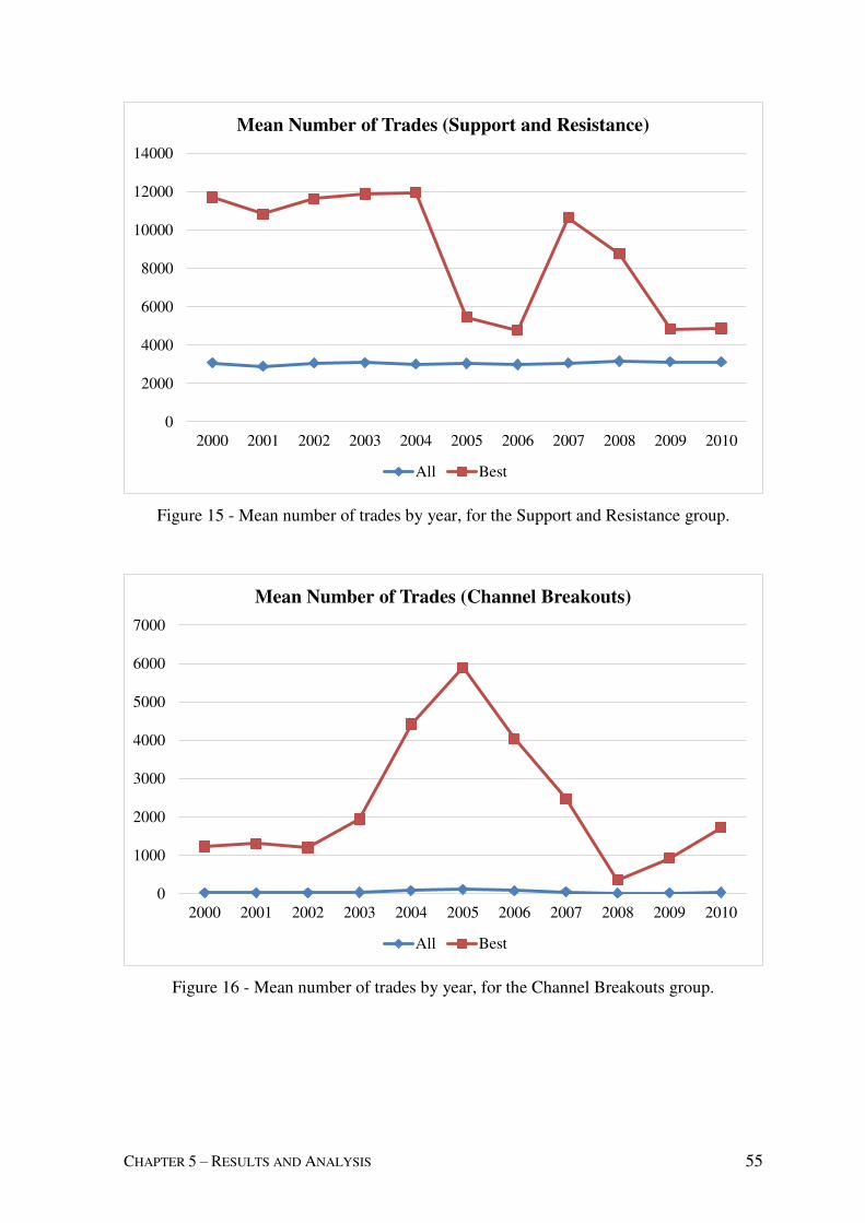
CHAPTER 5 – RESULTS AND ANALYSIS 55
Figure 15 - Mean number of trades by year, for the Support and Resistance group.
Figure 16 - Mean number of trades by year, for the Channel Breakouts group.
0
2000
4000
6000
8000
10000
12000
14000
2000 2001 2002 2003 2004 2005 2006 2007 2008 2009 2010
Mean Number of Trades (Support and Resistance)
All Best
0
1000
2000
3000
4000
5000
6000
7000
2000 2001 2002 2003 2004 2005 2006 2007 2008 2009 2010
Mean Number of Trades (Channel Breakouts)
All Best

56 CHAPTER 5 - RESULTS AND ANALYSIS
5.1.4. Number of winning and losing trades
In this section I analyze the number of trades where the trading rules generate positive
returns, from now on referred as winning trades, and when trades generate negative
returns, entitled, from now on, as losing trades.
In fact, Figure 17 shows that, in most years, the average winning filter rules use fewer
transactions than the rule, from that subgroup, which generates higher returns. The same is
also true for the losing trades, the average number of trades for the entire losing rules, for
most years, are less than the ones used by the best rule of the losing rules.
These conclusions are in line with the ones obtained from the previous analysis on the
number of trades. The best trading rules tend to use more transactions.
Having said that, the one different conclusion that can be drawn from the current analysis
is that the winning trades undergo, on average, on fewer trades than the loosing ones. The
same is relatable to the best trade in each situation (losing and winning), the best rule of the
winning trades uses, on average, less trades than the best rule of the losing trades, in each
year.
Regarding the other families of trading rules the results are similar (Figure 18, Figure 19
and Figure 20), with the channel breakouts, presented on Figure 20, the only exception.
Indeed, the channel breakouts winning trades, both for the entire group and the best rule,
have more transactions than the average for the losing trades.
CHAPTER 5 – RESULTS AND ANALYSIS 57
Figure 17 - Mean number of winning/losing trades by year, for the Filter Rules group.
Figure 18 - Mean number of winning/losing trades by year, for the Moving Averages
group.
0
1000
2000
3000
4000
5000
6000
7000
8000
2000 2001 2002 2003 2004 2005 2006 2007 2008 2009 2010
Mean Number of Winning/Losing Trades (Filter Rules)
All Winning Trades All Losing Trades
Best Winning Trades Best Losing Trades
0
500
1000
1500
2000
2500
3000
3500
2000 2001 2002 2003 2004 2005 2006 2007 2008 2009 2010
Mean Number of Winning/Losing Trades (Moving Averages)
All Winning Trades All Losing Trades
Best Winning Trades Best Losing Trades

58 CHAPTER 5 - RESULTS AND ANALYSIS
Figure 19 - Mean number of winning/losing trades by year, for the Support and Resistance
group.
Figure 20 - Mean number of winning/losing trades by year, for the Channel Breakouts
group.
0
500
1000
1500
2000
2500
3000
3500
4000
4500
2000 2001 2002 2003 2004 2005 2006 2007 2008 2009 2010
Mean Number of Winning/Losing Trades (Support and
Resistance)
All Winning Trades All Losing Trades
Best Winning Trades Best Losing Trades
0
500
1000
1500
2000
2500
3000
3500
2000 2001 2002 2003 2004 2005 2006 2007 2008 2009 2010
Mean Number of Winning/Losing Trades (Channel
Breakouts)
All Winning Trades All Losing Trades
Best Winning Trades Best Losing Trades

CHAPTER 5 – RESULTS AND ANALYSIS 59
5.1.5. Returns
The analysis of the mean returns per group of rules allows to easily deduce that most rules
start by having positive and (mostly) constant average returns, in the first three years, but
decrease afterwards, and, in some cases, they experience a new growth in 2008.
In specific, this trend is seen on the filter rules (Figure 21), on the moving averages (Figure
22) and on the support and resistance (Figure 23). The only exceptions to what has been
said is the average for the entire set of rules for the moving averages and the channel
breakouts, which register an annual value close to or equal to zero for most years, and the
best rules average for the channel breakouts which records the opposite behavior compared
to the other groups.
Figure 21 – Mean return by year, for the Filter Rules group.
-1,0E-06
0,0E+00
1,0E-06
2,0E-06
3,0E-06
4,0E-06
5,0E-06
6,0E-06
7,0E-06
8,0E-06
9,0E-06
2000 2001 2002 2003 2004 2005 2006 2007 2008 2009 2010
Mean Return (Filter Rules)
All Best

60 CHAPTER 5 - RESULTS AND ANALYSIS
Figure 22 - Mean return by year, for the Moving Averages group.
Figure 23 - Mean return by year, for the Support and Resistance group.
-1,0E-06
0,0E+00
1,0E-06
2,0E-06
3,0E-06
4,0E-06
5,0E-06
2000 2001 2002 2003 2004 2005 2006 2007 2008 2009 2010
Mean Return (Moving Averages)
All Best
0,0E+00
5,0E-07
1,0E-06
1,5E-06
2,0E-06
2,5E-06
3,0E-06
3,5E-06
4,0E-06
4,5E-06
5,0E-06
2000 2001 2002 2003 2004 2005 2006 2007 2008 2009 2010
Mean Return (Support and Resistance)
All Best

CHAPTER 5 – RESULTS AND ANALYSIS 61
Figure 24 - Mean return by year, for the Channel Breakouts group.
5.2. Superior Predictive Ability test
The results obtained from the SPA test, presented on Table 5, allow to conclude that the
null hypothesis is not rejected for any level (10, 5 or 1%) and over any of the sub-periods
(years) analyzed.
Indeed, the consistent value assumes its lowest value in the year of 2005, even though,
being higher than 60%. In all other years, and in the entire period, the consistent value is
around 80%.
Therefore no rule appears to be able to provide an average return statistically higher than
the one given by a buy and hold strategy.
0,0E+00
5,0E-07
1,0E-06
1,5E-06
2,0E-06
2,5E-06
3,0E-06
3,5E-06
4,0E-06
4,5E-06
5,0E-06
2000 2001 2002 2003 2004 2005 2006 2007 2008 2009 2010
Mean Return (Channel Breakouts)
All Best

62 CHAPTER 5 - RESULTS AND ANALYSIS
Table 5 - SPA test results.
Year Consistent Lower Upper
2000 0.848 0.000 1.000
2001 0.854 0.016 1.000
2002 0.775 0.008 1.000
2003 0.855 0.002 1.000
2004 0.833 0.021 0.987
2005 0.611 0.016 0.650
2006 0.773 0.014 0.926
2007 0.882 0.087 0.986
2008 0.871 0.228 1.000
2009 0.752 0.028 0.810
2010 0.844 0.078 0.929
All 0.974 0.000 1.000

CHAPTER 6 – CONCLUSIONS AND SUGGESTIONS FOR FUTURE WORK 63
CHAPTER 6
6. CONCLUSIONS AND SUGGESTIONS FOR FUTURE WORK
Given the state of the art on this topic, and despite the ongoing debate, from the start my
expectation was that technical trading rules would not be profitable even under a high-
frequency time frame.
Nonetheless, more than 60 years after the first endeavors in this area there is still a lot of
discussion on the topic.
In addition, the literature on intraday technical trading alludes to a few simple conclusions.
Such studies are relative recent, most of them, probably due to technical difficulties, use
datasets no longer than one year, and most of them do not employ robustness tests.
This study adds to the current literature by analyzing a substantially larger period of
intraday data than previous studies, and by comparing the trading rules using the Superior
Predictive Ability test (Hansen, 2005) to account for data snooping.
6.1. Conclusions
The results obtained do not leave much margin to interpretation. The fact is that the 5680
technical trading rules tested do not generate abnormal returns. This attests for the
efficiency of prices of the FTSE 100 index on the 11 years from January 2000 to December
2010.
Effectively, this is a conclusion obtained even without the consideration of transaction
costs. The results obtained prior to the consideration of the SPA test by Hansen (2005),
already seem to indicate that the rules tested do not outperform the market. The robustness
test confirmed that, and the consideration of taxes and fees would only reinforce the
results.
Indeed, comparing to existing studies on this subject, at least the ones that account for data
snooping and conduct, up to date, robustness tests, the conclusion is similar. The random
walk hypothesis and the EMH hold.

64 CHAPTER 6 – CONCLUSIONS AND SUGGESTIONS FOR FUTURE WORK
Marshall et al. (2008), Duvignage et al. (2013) and Chaboud et al. (2014) are examples of
studies that conduct similar tests over different markets/indexes with the consideration of
data snooping measures, leading to the same conclusions.
Studies like Wood et al. (1985), Los (1999), Busse and Green (2002), Cassese and
Guidolin (2004), Chordia et al. (2005) and Manahov et al. (2014), besides being conducted
on intraday datasets, they all have in common the fact that they state that markets are in
some way inefficient and the non inclusion of robustness tests to their results, or the
inclusion of outdated tests that are not the best to account for the results, overall,
significance.
In fact, here lies one of the most important achievements of this study, not only it provides
evidence that FTSE 100 index price incorporates historical information, but also uses a
robust test methodology. Being that the most likely cause for obtaining different results
from similar studies.
In addition, the analysis made on the duration and number of trades prompts a great insight
on the value of most, if not all, technical trading rules tested. The fact is that for all groups
of rules tested the best performing rule has much less time of exposure than the average for
all rules. This means that the less time a portfolio is on the market for a given rule, the
better is its performance.
In fact, this can be indicative that the technical trading rules tested don’t generate value on
their own merits, but their results may simply be due to luck and to a small exposure to the
market. If that was not the case and if indeed the rules tended to increase value when used,
the more time of usage the higher would be their returns, or at least its performance would
not exhibit such a notorious inversely correlated pattern.
6.2. Suggestions for future research
Even though the work accomplished was beyond the initial expectations, the technical
challenges that derived from working with such a large dataset of returns and rules
prevented me to explore the results even further.
Although the current work makes a small contribution to the state of the art on the field of
finance, in the sense it confirms the validity of the weak form of the EMH and the random
walk hypothesis on an intraday dataset and using the SPA test, there is still a lot of room to
improve this study in the future.

CHAPTER 6 – CONCLUSIONS AND SUGGESTIONS FOR FUTURE WORK 65
Firstly, the current study uses an index, and this is not a traded financial instrument, and
consequently these results would not be easily replicated in practice by an investor. So, the
usage of data from a tradable asset would be a substantial advantage.
Secondly, a different set of technical trading rules could be used. Although the rules used
in this study are fairly comprehensive, encompassing the most number of rules used in past
research, some recent studies point out other types of rules that can be used. For example, a
dynamic process to find trading rules can be used, in which an iterative process finds in
each step the best combination of single parameters to be used on a given rule for it to
achieve better performance.


REFERENCES 67
REFERENCES
Allen, H., & Taylor, M. (1992). The use of technical analysis in the foreign exchange
market. Journal of International Money and Finance, 113, 301–314.
Alexander, S. (1961). Price movements in speculative markets: trends or random walks.
Industrial Management Review, 2(2), 7–26.
Alexander, S. (1964). Price movements in speculative markets: trends or random walks,
no. 2. Industrial Management Review, 5(2), 25–46.
Bajgrowicz, P., & Scaillet, O. (2012). Technical trading revisited: False discoveries,
persistence tests, and transaction costs. Journal of Financial Economics, 106, 473-491.
Ball, R. (1978). Anomalies in relationships between securities’ yields and yield-surrogates.
Journal of Financial Economics, 6(2–3), 103–126.
Barclay, M., & Litzenberger, R. (1988). Announcement effects of new equity issues and
the use of intraday price data. Journal of Financial Economics, 21, 71–99.
Beja, A. (1977). The limits of price information in market processes. Working paper 61,
University of California, Berkeley, USA. Research Program in Finance.
Bekaert, G., & Hodrick, R. J. (1992). Characterizing predictable components in excess
returns on equity and foreign exchange markets. The Journal of Finance, 47(2), 467–509.
Berger, J., & Mandelbrot, B. (1963). A new model for error clustering in telephone
circuits. IBM Journal of Research and Development, 7(3), 224–236.
Bernstein, P. (1992). Capital ideas: the improbable origins of modern Wall Street. The Free
Press, New York, USA.
Bernstein, P. (1999). A new look at the efficient market hypothesis. The Journal of
Portfolio Management, 25(2), 1– 2.
Black, F. (1986). Noise. The Journal of Finance, 41(3), 529–543.
Brock, W., Lakonishok, J., & LeBaron, B. (1992). Simple technical trading rules and the
stochastic properties of stock returns. Journal of Finance, 47(5), 1731-1764.
Busse, J., & Green, T. (2002). Market efficiency in real time. Journal of Financial
Economics, 65, 415–437.
Carter, R., & Van Auken, H. (1990). Security analysis and portfolio management: a survey
and analysis. Journal of Portfolio Management, 81–85 Spring.
Cassese, G., & Guidolin, M. (2004). Pricing and informational efficiency of the MIB30
index options market. An analysis with high-frequency data. Economic Notes by Banca
Monte dei Paschi di Siena SpA, 33(2), 275-321.

68 REFERENCES
Chaboud, A., Chiquoine, B., Hjalmarsson, E., & Vega, C. (2014). Rise of the machines:
algorithmic trading in the Foreign Exchange market. The Journal of Finance, 69(5), 2045-
2084.
Chan, L., Gup, B., & Pan, M. (1997). International stock market efficiency and integration:
A study of eighteen nations. Journal of Business Finance & Accounting, 24(6), 803–813.
Chan, L., Jegadeesh, N., & Lakonishok, J. (1996). Momentum strategies. The Journal of
Finance, 51(5), 1681– 1713.
Chang, K. & Osler, C. (1999). Methodical madness: technical analysis and the irrationality
of exchange-rate forecasts. Economic Journal, 109 (458), 636-661.
Chen, S., & Yeh, C. (2002). On the emergent properties of artificial stock markets: the
efficient market hypothesis and the rational expectations hypothesis. Journal of Economic
Behavior & Organization, 49(2), 217– 239.
Chopra, N., Lakonishok, J., & Ritter, J. (1992). Measuring abnormal performance: do
stocks overreact? Journal of Financial Economics, 31(2), 235–268.
Chordia, T., Roll, R., & Subrahmanyam, A. (2008). Liquidity and the market efficiency.
Journal of Financial Economics, 87, 249-268.
Chung, D., & Hrazdil, K. (2010). Liquidity and market efficiency: analysis of NASDAQ
firms. Global Finance Journal, 21, 262-274.
Cootner, P. (1962). Stock prices: random vs. systematic changes. Industrial Management
Review, 3(2), 24–45.
Cutler, D., Poterba, J., & Summers, L. (1989). What moves stock prices? The Journal of
Portfolio Management, 15(3), 4–12.
De Bondt,W., & Thaler, R. (1985). Does the stock market overreact? The Journal of
Finance, 40(3), 793–805.
Diebold, F. & Mariano, R. (1995). Comparing predictive accuracy. Journal of Business
and Economic Statistics, 13: 253-63.
Dimson, E. & Marsh, P (1990). Volatility forecasting without data-snooping. Journal of
Banking and Finance, 14(2-3), 399-421.
Dimson, E., & Mussavian, M. (1998). A brief history of market efficiency. European
Financial Management, 4(1), 91–193.
Dimson, E., & Mussavian, M. (2000). Market efficiency. In The Current State of Business
Disciplines, edited by Dahiyva, Bhagwan Shri, 959-970. Roihtak: Spelbound.

REFERENCES 69
Duvinage, M., Mazza, P., & Petitjean, M (2013). The intra-day performance of market
timing strategies and trading systems based on Japanese candlesticks. Quantative Finance,
13(7), 1059-1070.
Eun, C., & Shim, S. (1989). International transmission of stock market movements. The
Journal of Financial and Quantitative Analysis, 24(2), 241–256.
Fama, E. (1963). Mandelbrot and the stable paretian hypothesis. The Journal of Business,
36(4), 420–429.
Fama, E. (1965). The behavior of stock-market prices. Journal of Business, 38(1), 34–105.
Fama, E. (1970). Efficient capital markets: a review of theory and empirical work. The
Journal of Finance, 25(2), 383–417.
Fama, E. (1976). Foundations of finance: portfolio decisions and securities prices. Basic
Books. New York, USA.
Fama, E. (1991). Efficient capital markets: II. The Journal of Finance, 46(5), 1575–1617.
Fama, E. (1998). Market efficiency, long-term returns, and behavioral finance. Journal of
Financial Economics, 49(3), 283–306.
Fama, E. & Blume, M. (1966). Filter rules and stock-market trading. Journal of Business,
39, 226-241.
Fama, E., Fisher, L., Jensen, M., & Roll, R. (1969). The adjustment of stock prices to new
information. International Economic Review, 10(1), 1–21.
Fama, E., & French, K. (1988). Permanent and temporary components of stock prices.
Journal of Political Economy, 96(2), 246-273.
Farmer, J., & Lo, A. (1999). Frontiers of finance: evolution and efficient markets.
Proceedings of the National Academy of Sciences of the United States of America, 96(18),
9991–9992.
French, K., & Roll, R. (1986). Stock return variances: the arrival of information and the
reaction of traders. Journal of Financial Economics, 17(1), 5–26.
Friedman, M. (1953). The case for flexible exchange rates. in M. Friedman (ed.). Essays in
positive economics. University of Chicago Press, Chicago, USA, pp.157–203.
Froot, K., & Perold, A. (1995). New trading practices and short-run market efficiency.
Journal of Futures Markets, 15(7), 731-766.
Giacomini, R. & White, H. (2003). Tests of conditional predictive ability. Working Paper
No. 572, Boston College, Boston, USA.
Godfrey, M., & Granger, C., & Morgenstern, O. (1964). The random walk hypothesis of
stock market behavior. Kyklos, 17(1), 1–30.

70 REFERENCES
Granger, C., & Morgenstern, O. (1963). Spectral analysis of New York stock market
prices. Kyklos, 16(1), 1–27. Reprinted in The Random Character of Stock Market Prices,
edited by P. H. Cootner, The MIT Press, Cambridge, MA, USA.
Granger, C., & Morgenstern, O. (1970). Predictability of stock market prices. Heath
Lexington Books. Lexington, MA, USA.
Grossman, S. (1976). On the efficiency of competitive stock markets where traders have
diverse information. The Journal of Finance, 31(2), 573–585.
Grossman, S., & Stiglitz, J. (1980). On the impossibility of informationally efficient
markets. The American Economic Review, 70(3), 393–408.
Hamilton, W. (1922). The stock market barometer. Harper and Brothers Publishers, New
York, USA.
Hansen, P. (2005). A Test for superior predictive ability. Journal of Business and
Economic Statistics, 23(4), 365-380.
Haugen, R. (1995). The new finance: the case against efficient markets. Contemporary
Issues in Finance. Prentice Hall, Englewood Cliffs, NJ, USA.
Haugen, R. (1999). The new finance: the case against efficient markets. Second edition.
Prentice Hall, Upper Saddle River, NJ, USA.
Hotchkiss, E., & Ronen, T. (2002). The informational efficiency of the corporate bond
market: an intraday analysis. The Review of Financial Studies, 15(5), 1325-1354.
Houthakker, H. (1961). Systematic and random elements in short-term price movements.
The American Economic Review, 51(2), 164–172.
Huang, R., & Stoll, H. (1994). Market microstructure and stock return predictions. The
Review of Financial Studies, 7(1), 179–213.
Jegadeesh, N. (1990). Evidence of predictable behavior of security returns. The Journal of
Finance, 45(3), 881–898.
Jegadeesh, N. (2000). Discussion. The Journal of Finance, 55(4), 1765–1770.
Jegadeesh, N., & Titman, S. (1993). Returns to buying winners and selling losers:
Implications for stock market efficiency. The Journal of Finance, 48(1), 65–91.
Jensen, M. (1978). Some anomalous evidence regarding market efficiency. Journal of
Financial Economics, 6(2), 95-101.
Keim, D., & Stambaugh, R. (1986). Predicting returns in stock and bond markets. Journal
of Financial Economics, 17, 357-390.
Kemp, A., & Reid, G. (1971). The random walk hypothesis and the recent behaviour of
equity prices in Britain. Economica, 38(149), 28–51.

REFERENCES 71
Kendall, M. (1953). The analysis of economic time-series—Part I: prices. Journal of the
Royal Statistical Society, 116(1), 11–25.
Keynes, J. (1936). The general theory of employment, interest and money. Harcourt,
Brace, New York, USA, chapter 12.
Laffont, J., & Maskin, E. (1990). The efficient market hypothesis and insider trading on the
stock market. Journal of Political Economy, 98(1), 70–93.
Lakonishok, J., & Smidt, S. (1988). Are seasonal anomalies real? A ninety year
perspective. Review of Financial Studies 3, 431-467.
Leamer, E. (1978). Specification searches. Wiley, New York, USA.
Lee, C., Lee, J., & Lee, C. (2010). Stock prices and the efficient market hypothesis:
evidence from a panel stationary test with structural breaks. Japan and the World
Economy, 22(1), 49–58.
Lehmann, B. (1990). Fads, martingales, and market efficiency. The Quarterly Journal of
Economics, 105(1), 1–28.
LeRoy, S., & Porter, R. (1981). The present-value relation: Tests based on implied
variance bounds. Econometrica, 49(3), 555–574.
Levich, R., & Thomas, L. (1993). The significance of technical trading rules in the foreign
exchange market: A bootstrap approach. Journal of International Money and Finance, 12,
451-474.
Lewellen, J., & Shanken, J. (2002). Learning, asset-pricing tests, and market efficiency.
The Journal of Finance, 57(3), 1113–1145.
Lo, A. (1997). Market efficiency: stock market behaviour in theory and practice. The
International Library of Critical Writings in Financial Economics, Elgar, Cheltenham, UK.
Lo, A. (2008). Efficient markets hypothesis, in S. N. Durlauf and L. E. Blume (ed.). The
New Palgrave Dictionary of Economics, second edition. Palgrave Macmillan, London,
UK.
Lo, A., & MacKinlay, A. (1988). Stock market prices do not follow random walks:
evidence from a simple specification test. The Review of Financial Studies, 1, 41-66.
Lo, A., & MacKinlay, A. (1990). Data-snooping biases in tests of financial asset pricing
models. Review of Financial Studies 3, 431-467.
Lo, A, & MacKinlay, A. (1999). A non-random walk down Wall Street. Princeton
University Press, Princeton, NJ, USA.

72 REFERENCES
Lo, A., & Mamaysky, H., and Wang, J. (2000). Foundations of technical analysis:
computational algorithms, statistical inference, and empirical implementation. The Journal
of Finance, 55(4), 1705–1770.
London Stock Exchange Group.(2016, Nov. 15) Official website of the London stock
exchange, FTSE 100 index official information. Consulted on November 15, 2016.
Available at http://www.londonstockexchange.com/traders-and-brokers/rules-
regulations/core-rules/core-rules.htm.
Los, C. (1999). Nonparametric Testing of the High-Frequency Efficiency of the 1997
Asian Foreign Exchange Markets. Journal of Multinational Financial Management, 9,
265-289.
Lui, Y., & Mole, D. (1998). The use of fundamental and technical analysis by foreign
exchange dealers: Hong Kong evidence. Journal of International Money and Finance, 17,
535–545.
Malkiel, B. (1973). A random walk down Wall Street. Norton, New York, USA.
Malkiel, B (1981). A random walk down Wall Street, 2ed. Norton, New York, USA.
Malkiel, B. (1992). Efficient market hypothesis. In P. Newman, M. Milgate and J. Eatwell
(eds.), New Palgrave Dictionary of Money and Finance, Macmillan, London, UK.
Malkiel, B. (2003). The efficient market hypothesis and its critics. The Journal of
Economic Perspectives, 17(1), 58-82.
Manahov, V., Hudson, R., & Gebka, B. (2014). Does high frequency trading affect
technical analysis and market efficiency? And if So, How? Journal of International
Financial Markets, Institutions & Money, 28, 131-157.
Mandelbrot, B. (1962). The variation of certain speculative prices. Research Note NC-87,
IBM.
Mandelbrot, B. (1966). Forecasts of future prices, unbiased markets, and “martingale”
models. Journal of Business, 39(1), 242–255.
Marshall, B., Cahan, R., & Cahan, J. (2008). Does intraday technical analysis in the US
equity market have value? Journal of Empirical Finance, 15, 199-210.
Metcalf, G., & Malkiel, B. (1994). The Wall Street Journal contests: the experts, the darts,
and the efficient market hypothesis. Applied Financial Economics, 4(5), 371–374.
Oberlenchner, T. (2001). Importance of technical and fundamental analysis in the
European foreign exchange market. International Journal of Finance and Economics, 6,
81–93.

REFERENCES 73
Osborne, M. (1962). Periodic structure in the Brownian motion of stock prices. Operations
Research, 10(3), 345–379.
Pesaran, M., & Timmerman, A. (1995). Predictability of stock returns: robustness and
economic significance. Journal of Finance 28, 85-105.
Politis, D. & Romano, J. (1994). The stationarity bootstrap. Journal of the American
Statistical Association, 89, 1303-1313.
Rhea, R. (1932). The Dow Theory. Fraser Publishing, Burlington, Vermont, USA.
Roberts, H. (1967). Statistical versus clinical prediction of the stock market. Unpublished
manuscript.
Roll, R. (1984). Orange juice and weather. The American Economic Review, 74(5), 861–
880.
Samuelson, P. (1965). Proof that properly anticipated prices fluctuate randomly. Industrial
Management Review, 6(2), 41–49.
Samuelson, P. (1973). Proof that properly discounted present values of assets vibrate
randomly. The Bell Journal of Economics and Management Science, 4(2), 369–374.
Schwert, G. (2002). Anomalies and market efficiency. Working paper 9277, Simon School
of Business, University of Rochester, Rochester, New York, USA.
Scholtus, M., & van Dijk, D. (2012). High-frequency technical trading: the importance of
speed. Econometric Institute and Tinbergen Institute, Erasmus University, Rotterdam,
Netherlands.
Sewell, M. (2011). History of the efficient market hypothesis. Research note 11/04.
Department of Computer Science, University College London, London, UK.
Shiller, R. (1981). Do stock prices move too much to be justified by subsequent changes in
dividends? The American Economic Review, 71(3), 421-436.
Shiller, R. (1989). Market volatility. The MIT Press, Cambridge, MA, USA.
Shiller, R. (2000). Irrational exuberance. Princeton University Press, Princeton, NJ, USA.
Shleifer, A. (2000). Inefficient markets: an introduction to behavioral finance. Oxford
University Press, Oxford, UK.
Steiger, W. (1964). A test of nonrandomness in stock price changes. in P. H. Cootner (ed.),
The random character of stock market prices. The MIT Press, Cambridge, MA, USA.
Chapter XII, 303–312.
Stiglitz, J. (1981). The allocation role of the stock market: Pareto optimality and
competition. The Journal of Finance, 36(2), 235–251.

74 REFERENCES
Sullivan, R., Timmermann, A., & White, H. (1999). Data-snooping, technical trading rules
performance, and the bootstrap. Journal of Finance, 245, 1647–1691.
Sullivan, R., Timmermann, A., & White, H. (2001). Dangers of data mining: The case of
calendar effects in stock returns. Journal of Econometrics, 105, 249–286.
Summers, L. (1986). Does the stock market rationally reflect fundamental values? The
Journal of Finance, 41(3), 591–601.
UK Government. (2016, Nov. 15) Official website of the UK government services and
information. Consulted on November 15, 2016. Available at https://www.gov.uk/bank-
holidays.
Wilson, E., & Marashdeh, H. (2007). Are co-integrated stock prices consistent with the
efficient market hypothesis? The Economic Record, 83(1), 87–93.
White, H. (2000). A reality check for data snooping. Econometrica, 68(5), 1097–1126.
Wood, R., McInish, T., & Ord, J. (1985). An investigation of transactions data for NYSE
stocks. The Journal of Finance, 40(3), 723-739.
Yen, G., & Lee, C. (2008). Efficient market hypothesis (EMH): past, present and future.
Review of Pacific Basin Financial Markets and Policies, 11(2), 305–329.

APPENDIX 75
APPENDIX
Appendix 1 – Observations out of chronological order (eliminated from
the dataset).
Date Time Price Date Time Price Date Time Price
30/11/2009 08:00:54 5256.98 30/11/2009 10:00:45 5206.28 30/11/2009 11:36:27 5207.99
30/11/2009 08:00:57 5261.92 30/11/2009 10:02:52 5208.25 30/11/2009 11:37:01 5210.29
30/11/2009 08:01:23 5255.43 30/11/2009 10:03:38 5209.54 30/11/2009 11:47:09 5206.92
30/11/2009 08:01:24 5255.43 30/11/2009 10:04:31 5209.84 30/11/2009 11:54:31 5208.29
30/11/2009 08:02:41 5255.16 30/11/2009 10:07:09 5208.39 30/11/2009 11:55:27 5208.26
30/11/2009 08:02:52 5255.28 30/11/2009 10:10:15 5205.07 30/11/2009 11:59:36 5207.62
30/11/2009 08:04:01 5257.12 30/11/2009 10:12:22 5206.47 30/11/2009 12:00:02 5208.32
30/11/2009 08:04:28 5258.34 30/11/2009 10:12:27 5206.81 30/11/2009 12:00:03 5208.51
30/11/2009 08:04:30 5258.51 30/11/2009 10:13:09 5207.06 30/11/2009 12:00:05 5208.54
30/11/2009 08:09:17 5252.79 30/11/2009 10:16:28 5196.70 30/11/2009 12:00:06 5208.60
30/11/2009 08:13:44 5252.56 30/11/2009 10:20:05 5195.92 30/11/2009 12:00:08 5208.75
30/11/2009 08:14:15 5250.02 30/11/2009 10:22:58 5199.50 30/11/2009 12:11:24 5206.58
30/11/2009 08:16:10 5233.71 30/11/2009 10:26:13 5192.10 30/11/2009 12:12:39 5205.41
30/11/2009 08:16:23 5232.89 30/11/2009 10:26:31 5192.64 30/11/2009 12:14:36 5207.62
30/11/2009 08:16:55 5233.14 30/11/2009 10:35:02 5203.75 30/11/2009 12:31:49 5196.66
30/11/2009 08:17:23 5229.98 30/11/2009 10:37:21 5204.75 30/11/2009 12:41:56 5200.06
30/11/2009 08:21:03 5226.93 30/11/2009 10:40:22 5216.45 30/11/2009 12:52:01 5198.58
30/11/2009 08:21:15 5227.54 30/11/2009 10:43:31 5215.16 30/11/2009 13:05:03 5205.37
30/11/2009 08:22:45 5222.26 30/11/2009 10:47:24 5212.19 30/11/2009 13:05:07 5205.48
30/11/2009 08:26:24 5224.33 30/11/2009 10:48:40 5213.46 30/11/2009 13:19:31 5209.64
30/11/2009 08:37:41 5217.96 30/11/2009 10:51:09 5210.99 30/11/2009 13:25:57 5217.22
30/11/2009 08:46:39 5218.88 30/11/2009 10:52:21 5209.92 30/11/2009 13:59:58 5212.20
30/11/2009 08:56:34 5226.10 30/11/2009 10:59:12 5211.35 30/11/2009 14:21:50 5207.38
30/11/2009 09:32:24 5214.44 30/11/2009 11:10:35 5199.85 30/11/2009 14:31:01 5216.86
30/11/2009 09:35:15 5217.63 30/11/2009 11:12:52 5197.10 30/11/2009 15:02:01 5227.71
30/11/2009 09:40:23 5212.91 30/11/2009 11:16:12 5198.88 30/11/2009 16:27:29 5199.45
30/11/2009 10:00:37 5204.93 30/11/2009 11:17:56 5198.20 27/04/2010 14:40:11 5671.88
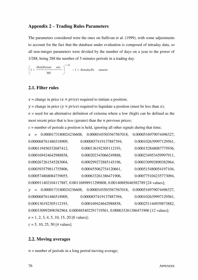
76 APPENDIX
Appendix 2 – Trading Rules Parameters
The parameters considered were the ones on Sullivan et al. (1999), with some adjustments
to account for the fact that the database under evaluation is composed of intraday data, so
all non-integer parameters were divided by the number of days on a year to the power of
1/288, being 288 the number of 5 minutes periods in a trading day.
rameterIntradayPaeterDailyParam
1
3651
288/1
2.1. Filter rules
= change in price ( × ��� ) required to initiate a position;
= change in price ( × ��� ) required to liquidate a position (must be less than );
= used for an alternative definition of extrema where a low (high) can be defined as the
most recent price that is less (greater) than the previous prices;
= number of periods a position is held, ignoring all other signals during that time;
= 0.0000173180024236608, 0.0000345503567567018, 0.0000516979074496327,
0.000068761486518909, 0.0000857419137887394, 0.000102639997129561,
0.000119456532687412, 0.000136192305112193, 0.000152848087775936,
0.000169424642988858, 0.000202343066249888, 0.000234953459997911,
0.000267261545283004, 0.000299272885145196, 0.000330992890382964,
0.000393579811755806, 0.000455062754120661, 0.000515480054197104,
0.000574868084739055, 0.000633261386471906, 0.000775104235773094,
0.000911402104117887, 0.00116898911290808, 0.00140885646582789 [24 values];
= 0.0000173180024236608, 0.0000345503567567018, 0.0000516979074496327,
0.000068761486518909, 0.0000857419137887394, 0.000102639997129561,
0.000136192305112193, 0.000169424642988858, 0.000251144939873882,
0.000330992890382964, 0.000485402291719561, 0.000633261386471906 [12 values];
= 1, 2, 3, 4, 5, 10, 15, 20 [8 values];
= 5, 10, 25, 50 [4 values].
2.2. Moving averages
= number of periods in a long period moving average;

APPENDIX 77
= number of periods in a short period moving average;
= fixed band multiplicative value;
= number of periods for the time delay filter;
= number of periods a position is held, ignoring all other signals during that time;
= 5, 10, 15, 20, 25, 30, 40, 50, 75, 100, 125, 150, 200, 250 [14 values];
= 2, 5, 10, 15, 20, 25, 30, 40, 50, 75, 100, 125, 150, 200 [14 values];
= 0.0000034704932898, 0.0000173180024236608, 0.0000345503567567018,
0.0000516979074496327, 0.000068761486518909, 0.000102639997129561,
0.000136192305112193, 0.000169424642988858 [8 values];
= 2, 3, 4, 5 [4 values];
= 5, 10, 25, 50 [4 values].
2.3. Support and resistance
= number of periods in the support and resistance range;
= fixed band multiplicative value;
= number of periods for the time delay filter;
= number of periods a position is held, ignoring all other signals during that time;
= 5, 10, 15, 20, 25, 50, 100, 150, 200, 250 [10 values];
= 0.0000034704932898, 0.0000173180024236608, 0.0000345503567567018,
0.0000516979074496327, 0.000068761486518909, 0.000102639997129561,
0.000136192305112193, 0.000169424642988858 [8 values];
= 2, 3, 4, 5 [4 values];
= 5, 10, 25, 50 [4 values].
2.4. Channel Breakouts
= number of periods for the channel;
= difference between the high price and the low price ( × ��� ) required to form the
channel;
= number of periods for the time delay filter;
= number of periods a position is held, ignoring all other signals during that time;
= 5, 10, 15, 20, 25, 50, 100, 150, 200, 250 [10 values];

78 APPENDIX
= 0.0000173180024236608, 0.0000345503567567018, 0.000068761486518909,
0.000102639997129561, 0.000169424642988858, 0.000251144939873882,
0.000330992890382964, 0.000485402291719561 [8 values];
= 2, 3, 4, 5 [4 values];
= 5, 10, 25, 50 [4 values].